a note on the relationship between high-frequency trading

This is a repository copy of A note on the relationship between high-frequency trading and latency arbitrage.

White Rose Research Online URL for this paper:https://eprints.whiterose.ac.uk/117919/

Version: Accepted Version

Article:

Manahov, Viktor (2016) A note on the relationship between high-frequency trading and latency arbitrage. International Review of Financial Analysis. pp. 281-296. ISSN 1057-5219

https://doi.org/10.1016/j.irfa.2016.06.014

[email protected]://eprints.whiterose.ac.uk/

Reuse

This article is distributed under the terms of the Creative Commons Attribution-NonCommercial-NoDerivs (CC BY-NC-ND) licence. This licence only allows you to download this work and share it with others as long as you credit the authors, but you can’t change the article in any way or use it commercially. More information and the full terms of the licence here: https://creativecommons.org/licenses/

Takedown

If you consider content in White Rose Research Online to be in breach of UK law, please notify us by emailing [email protected] including the URL of the record and the reason for the withdrawal request.

1 | P a g e

A note on the Relationship between High-Frequency Trading and Latency

Arbitrage.

Abstract

We develop three artificial stock markets populated with two types of market participants – HFT

scalpers and aggressive high frequency traders (HFTrs). We simulate real-life trading at the

millisecond interval by applying Strongly Typed Genetic Programming (STGP) to real-time data from

Cisco Systems, Intel and Microsoft. We observe that HFT scalpers are able to calculate NASDAQ

NBBO (National Best Bid and Offer) at least 1.5 milliseconds ahead of the NASDAQ SIP (Security

Information Processor), resulting in a large number of latency arbitrage opportunities. We also

demonstrate that market efficiency is negatively affected by the latency arbitrage activity of HFT

scalpers, with no countervailing benefit in volatility or any other measured variable. To improve

market quality, and eliminate the socially wasteful arms race for speed, we propose batch auctions in

every 70 milliseconds of trading.

-----------------------------------------------------------------------------------------------------------------

Keywords: Agent-Based Modelling, High Frequency Trading, Algorithmic Trading, Market Regulation, Market

Efficiency, Genetic Programming.

JEL Classification: G10,G12, G14, G19

2 | P a g e

1.Introduction

Wissner-Gross and Freer (2010) suggest that the time light travels between antipodal points on the

surface of the Earth takes 67 milliseconds, while recent computational advances transform HFT

latencies below 500 microseconds (Bhupathi, 2010). Many HFT strategies are designed to exploit

advantages in latency – the time it takes to access and respond to market information (Wah and

Wellman, 2013). Schneider (2012) estimates that trading on latency advantages account for $21

billion profit each year. HFTrs are able to obtain such speed advantages over institutional investors by

developing sophisticated trading algorithms combined with co-located computer systems, directly

linked with trading venues. At the same time, market structure issues due to speed competition among

HFTrs create the unintended consequence of allowing faster traders to gain revenue from trading with

slower traders (McInish and Upson, 2013). The practice of HFT has generated several public

controversies regarding its transparency and the fairness of market operations, as well as its

implications for market quality (Wah and Wellman, 2013).

However, most of the empirical work on the topic lacks the ability to identify which trades and quotes

come from HFT, making it difficult to examine how HFT affects the market and other market

participants (Egginton et al., 2012; Hirschey, 2013; Goldstein et al., 2014). This is due to the fact that

no publicly available dataset, including NASDAQ 120, allows researchers to directly identify all HFT

(Baron et al., 2012). Egginton et al., (2012) argue that is hardly possible to identify orders generated

by computer algorithms in the U.S. equities markets, with all previous studies using proxies to

measure the level of algorithmic trading and HFT1. The huge number of variables and very

complicated cause-effect relationships among these variables and potential outcomes imposes another

research obstacle (Felker et al., 2014). Furthermore, empirically measuring informational differences

between different investors represents a difficult task as investors’ information sets are unobservable

(Ding et al., 2014).

1 Hendershott et al. (2011) and Viljoen et al. (2014) implement the rate of electronic message traffic normalised

by trading volume as proxies to identify specific HFT in the dataset. Brogaard et al. (2014) use proprietary data to detect specific HFT activity. Hendershott and Riordan (2013), Brogaard et al. (2013), and Baron et al. (2012) extract account- level trade-by trade data related to different contracts for grouping traders into different high frequency categories; these are, based on the level of their trading volume as well as inventory management.

3 | P a g e

In contrast, this study uses a special adaptive form of Strongly Typed Genetic Programming (STGP)

and real-time millisecond data from Cisco Systems, Intel and Microsoft to demonstrate the process of

latency arbitrage in HFT. The STGP (described in Appendix B) is a sophisticated and extremely

suitable trading algorithm that successfully replicates HFT scalping strategies. Wah and Wellman

(2013) argue that questions about HFT implications are inherently computational in nature due to the

fact that the speed of trading reveals details of internal market activities and the structure of

communication channels. We subscribe directly to NASDAQ’s Security Information System (SIP),

which is called the Unlisted Trading Privileges Quote Data Feed in order to reproduce the HFT

scalping strategies in an artificial stock market environment. Here, the impact of these strategies can

be examined and new regulations evaluated to maintain the overall health of the financial system.

Using STGP, we replicate the interactions between HFT scalpers and aggressive HFTrs and compare

their performance under the same underlying trading order streams. In other words, we simulate real-

life trading sessions, which allow us to avoid the obstacles in the studies discussed above. HFT

scalping strategies originated as relatively simple spread detecting tools that came to understand the

order book depth, posted on the best bid/ask and then moved quickly to the other side (Patterson,

2012). These straightforward flipping strategies evolved over time to become the modern HFT

scalping strategies that nowadays dominate electronic exchanges, gaining favourable queue positions

and generating a huge amount of cancelled orders. The aim of HFT scalping strategies is to gain a

favourable queue position – any particular scalping strategy must have a high probability of entering

the trade and an equally high probability of either exiting for spread or, if the spread cannot be gained,

of immediately exiting in order to avoid losses (Bodek, 2013).

To summarise, the contribution of this study is three-fold. First, this is the first study to use an

innovative trading algorithm and real-time millisecond data to provide empirical evidence of how

HFT scalping strategies are able to calculate NASDAQ NBBO (National Best Bid and Offer) at least

1.5 milliseconds ahead of the NASDAQ SIP, creating a large number of latency arbitrage

opportunities.

4 | P a g e

The Securities and Exchange Commission (SEC) developed the Regulation National Market System

(Reg NMS) in 2007 in order to protect fair access to the best stock price for traditional investors.

According to Reg NMS rules, trading venues are required to provide trading messages to the primary

exchanges such as NASDAQ and NYSE. The SIPs for NASDAQ, which are called Unlisted Trading

Privileges Quote Data Feed, along with NYSE’s Consolidated Quotation System, collect all relevant

data and calculate the respective NBBO. Consequently, stock brokers are required to execute trading

orders at NBBO prices or better (Ding et al.,2014). However, considering trading order information

from all exchanges, the SIPs take some finite time, let us say milliseconds, to calculate and for the

NBBO to be distributed. Computationally sophisticated traders equipped with front-running scalping

strategies such as HFT scalpers can process the order flow in less than milliseconds and out-

compute the SIP to calculate the NBBO. Under trading conditions of superhuman speed, quotes

within an exchange could update faster than the exchange is able to distribute its new prices to other

trading venues for NBBO evaluation. Our experiment detects the processing and calculation of both

best bid and ask orders; it does this by simulating the communication patterns between HFT scalpers,

aggressive HFTrs, NASDAQ SIPs and NASDAQ NBBO. Our empirical results demonstrate that the

ability of HFT scalpers to create latency arbitrage opportunities makes trading more difficult and

more costly for those traditional investors who lack access to sophisticated trading platforms.

Second, this study provides the first real-life trading evidence whereby direct access to exchanges and

appropriate trading software could generate profitable opportunities for HFT companies. We

demonstrate that HFTrs equipped with scalping trading mechanisms are capable of capturing

substantial risk-free profits at the expense of institutional investors. We also measure the precise level

of profits generated by HFT scalpers and the exact costs of latency arbitrage for other market

participants. Our findings suggest that there is an arms race in speed and how fast market participants

have to be to capture profit opportunities. The size of the arbitrage opportunity, and hence the harm to

institutional investors, may depend on the magnitude of speed and the cost of cutting-edge speed

improvements.

5 | P a g e

Third, we provide clear evidence of the implications of latency arbitrage for market quality and the

relationship between market fragmentation and latency arbitrage strategies.

Our empirical findings indicate that latency arbitrage not only reduces the profits of other market

participants, but harms market efficiency. We observe that HFT scalpers’ latency arbitrage activity

has negative implications on market efficiency as intraday volatility increases and market depth

decreases. We propose an alternative financial market mechanism such as a batch auctioned market,

which successfully eliminates latency arbitrage opportunities and improves efficiency. We suggest the

implementation of batch auctions once every 70 milliseconds, that is 334,285 times per 6.5-hour

trading day for each financial instrument. If trading orders are bunched together every 70

milliseconds, HFT scalpers could face a queuing risk leading to a less harmful market quality effect.

Our study is particularly timely as policymakers around the world are still debating as to whether HFT

is beneficial or harmful to market efficiency (Manahov et al., 2014). To a certain extent this study can

be seen as a tool assisting regulators in the more rigorous evaluation of the financial market.

The remainder of this paper is organised as follows: Section 2 comprises the literature review on the

topic. Section 3 presents the experimental design of the three artificial stock markets and data

description. In Section 4, we examine the HFT scalpers’ latency arbitrage activity and profitability

and investigate the implications of HFT scalpers on market quality and the associated regulatory

measures. Finally, Section 5 concludes the paper. Additional clarifying and technical material can be

found in Appendix A.

6 | P a g e

2.Related literature

While Ready (1999) and Stoll and Schenzler (2006) perform empirical analysis to show how slow

traders’ orders provide a free trading option for fast traders, Cohen and Szpruch (2012) consider a

single asset market model of latency arbitrage with one limit order book and two traders possessing

different speeds of trade execution. This is to demonstrate that the fast trader employs a front-running

strategy to capture the quantity that the slower trader intends to trade and generate a risk-free profit.

However, the authors suggest that these profits cannot be scaled and the introduction of a ‘Tobin Tax’

on financial transactions could lead to the elimination of profits from pre-emptive strategies. In

contrast, our study measures the exact level of profit that HFTrs gain from latency arbitrage.

Hirshleifer et al. (1994) examine trading behaviour and equilibrium information acquisition whereby

some investors receive common private information before others. Their model implies that under

some conditions better informed investors equipped with profit-taking strategies will focus only on a

subset of securities, while ignoring other securities with similar characteristics. In a similar fashion,

Foucault et al. (2013), model the strategic behaviour of a trader trading in public information faster

than other traders, demonstrating that with a speed advantage, the informed trader’s order flow is

much more volatile, accounts for a much bigger fraction of trading volume, and forecasts very short

run price changes. In a rather different laboratory experiment, Wah and Wellman (2013) adopted an

agent-based approach to simulate the interactions between high-frequency and zero-intelligence

agents at the millisecond level. Similar to our empirical findings, the authors reported that market

fragmentation and the presence of a latency arbitrageur reduces total surplus, leading to negative

implications for liquidity.

On 10th of March, 2008, the NYSE implemented a system upgrade designed to reduce its latency by

600 milliseconds. McInish and Upson (2013) use this event to investigate the implications of the

reduction in latency for trading quality. They observe that for trades executed at NBBO prices, order

execution quality improves significantly but faster markets reduce the ability of fast liquidity suppliers

to execute the quote-arbitrage strategy.

7 | P a g e

Easley et al. (2014), examine a different upgrade within the NYSE’s trading system which was

implemented to reduce the latency of off-floor traders and show that this reduction improves liquidity,

raising stock prices in comparison to that of on-floor traders. A portfolio consisting of long stocks that

is undergoing the upgrade has a return of approximately 3 percent over the first 20 days of the

upgrade. In another NBBO experiment, Ding et al. (2014), provide evidence as to the benefits of

obtaining faster proprietary data feeds from stock exchanges over the regulated public consolidated

data feeds. They measure and compare NBBO prices from each data feed to discover price

dislocations in the NBBO that occur several times a second and last one to two milliseconds

presenting opportunities for HFT latency arbitrage. The relatively short duration of dislocations is

associated with small cost for infrequent traders but prove costly for frequent traders.

Easley et al. (2012) argue that allowing exchanges to directly sell trade and quote data to some traders

increases the cost of capital and worsens market liquidity in comparison to trading where all market

participants freely observe previous prices. Moreover, allowing exchanges to sell price information is

undesirable because it has negative implications on market quality, therefore such practice should be

restricted.

However, most of the studies on the topic rely on empirical tests and statistical evaluation of

historical datasets. In contrast, we develop a more realistic scenario by simulating real-life trading

with real-time millisecond data in order to investigate the relationships between fast and slow traders

and the implications for market quality.

8 | P a g e

3.Experimental design

Due to advances in technology and the rapid growth of high frequency trading, financial markets have

eliminated human intermediation in the trading process and replaced them with electronic limit order

books, which have led to the growth of trading algorithms as one of the main investment tools. Some

of the trading algorithms generated imitate the behaviour of humans in the trading process, while over

the last few years, these trading algorithms have substantially improved their speed to match bid and

ask orders.

We use a special adaptive form of Strongly Typed Genetic Programming (STGP), which enables us to

choose and adjust different parameters to suit our specification, such as the minimum price increment,

number of participants and their wealth, the level of transaction costs, and different trading

preferences. The exact number of evolutionary parameters that we can specify is listed in Table 1.

Each market participant represents an artificial trader who is equipped with their own trading rule; the

selection of best performing traders and the production of new genomes is conducted through the

recombination of the parent genomes by crossover and mutation operations, which are further

elaborated upon in Appendices A and B. The basic idea is that the trader’s trading rule will improve

by a natural selection process based on the survival of the fittest (Witkam, 2014).

Therefore, the evolutionary nature of the trading process and the price dynamics enable the artificial

traders to recognise, learn and exploit profit opportunities while continually adapting to changing

market conditions. Consequently, the STGP trading algorithm evolves the model step-by-step, feeding

it with real-time millisecond quotes from Cisco Systems, Intel and Microsoft stocks; therefore the

forecasting models evolve mimicking the actual markets studied. Model evolution doesn’t end when

disconnected from the data feeder or when the quote file ends. It continues when new quotes are

added to the database and there is no difference between the way historical quotes and new quotes are

processed.

9 | P a g e

3.1. The process of developing initial trading rules

Each individual trader has only one trading rule which is created randomly, enabling the whole range

of possible trading rules to be studied (examples of trading rules can be found in Appendix B). To

create later generations, we apply the crossover recombination technique and mutation operation,

where the crossover recombination technique randomly chooses parts of two trading rules to exchange

in order to create two new trading rules; the mutation operation randomly changes a small part of a

trading rule. This process is repeated until at least one trading rule in the population achieves the

desired level of fitness, which is measured by a trader’s investment return over a specified period. It

should be noted that this initial random nature can result in the creation of meaningless trading rules

or trading rules which cannot be evaluated thoroughly since they do not return the value that the

function needs. Nevertheless, as Montana (1995) notes, these programming issues can be resolved by

the introduction of STGP, where the process requires the definition of a specific set to fit the problem.

Each trading rule in our artificial stock market setting takes real-time millisecond prices from Cisco

Systems, Intel and Microsoft and generates advice consisting of the desired position, estimated as a

percentage of the trader’s wealth, and an order limit price for buying and selling the financial

instrument2. The trading rules’ logic comprises of information on price and volume, minimum,

maximum and average functions related to millisecond price and trading volume data, as well as

different logical and comparison operators.

Moreover, traders are not allowed to directly communicate with each other in order to avoid herding

behaviour that occurs when copying the trading activity of other traders. However, traders are able to

indirectly exchange information through the artificial stock market and also through the breeding

process.

In the conventional Genetic Programming (GP) procedure, described in Appendix A, trading rules are

evaluated by the same fitness function in each generation. In contrasts, the STGP evaluates the fitness

of traders through a dynamic fitness function, which enables the return estimation period to move

forward and include the most recent quotes in the market.

2 This process is further explained in subsections 3.2 and 3.3.

10 | P a g e

Also, while GP replaces the entire genetic population through crossover and mutation techniques at

one time, STGP only replaces a small proportion of the entire population, which ensures a gradual

change in population and thus greater model stability (Witkam, 2014). Another important feature of

STGP is that each trader discovers the intrinsic value of the three stocks individually without any

communication between traders, ensuring individuality and that the level of intelligence of each

artificial trader is not affected by other traders. This allows the development of more meaningful

trading rules for both HFT scalpers and strategic informed traders.

3.2. Structure of the artificial stock market and the differences between HFT scalpers

and aggressive HFTrs.

We examine the profitability of HFT strategies within the context of a number of markets, each

populated by up to 100,000 boundedly rational traders. None of the artificial traders in the model are

orientated towards a predetermined formation of strategy and so are therefore free to develop and

continually evolve new and better trading rules over time. We develop three different artificial stock

markets for each of the three financial instruments under investigation. Each market is populated by

50,000 aggressive HFTrs and 50,000 HFT scalpers (50 per cent of the total population based on the

continuous Breeding Fitness Return). Both HFT scalpers and aggressive HFTrs are created using the

STGP programming technique explained in Appendix A. In terms of aggressive HFtrs’ design there is

an important difference between two features: the horizon or holding period, measured by the length

of time for which a position (long or short) is a financial instrument is held; and the trading costs

measured by the bid-ask spread that must be crossed by trading orders.

In order to generate profits, aggressive HFTrs must hold their positions for a sufficient period of time

in order to overcome the transaction cost. Hence, the shorter the holding period, the more extreme the

movements of price must be to ensure profitability. However, the main difference between the two

trading groups is that the HFT scalpers’ group consists of the traders who momentarily perform best

in terms of the continuous Breeding Fitness Return; these, therefore possess lower latency. The

Breeding Fitness Return is a trailing return of a wealth moving average which determines the fitness

rules of traders.

11 | P a g e

This return is calculated over the last n quotes of data of an exponential moving average of traders’

wealth, where n is set to the minimum breeding age with a maximum of 250. In the case where the

age is less than n, no value is calculated. This particular type of return is used to measure the fitness

criterion for the selection of traders to breed. Breeding is, in essence, a process of creating new

artificial traders to replace poor performing ones based on the values derived from Equation (1)

below. HFT scalpers and aggressive HFTrs process millisecond trading messages using direct data

feed from the NASDAQ SIP. Although HFT scalpers and aggressive HFTrs both observe the same

millisecond data from the three financial instruments and also generate trading orders, HFT scalpers

are able to access and process the data first due to their low latency features. In other words, HFT

scalpers are able to foresee the quotes of the three financial instruments and submit trading orders

before the contribution of aggressive HFTrs. Both HFT scalpers and aggressive HFTrs operate in the

same market and accumulate wealth by investing in two financial instruments that are available on the

artificial stock market; the three risky financial instruments and the risk-free instrument represented

by cash. Because the three artificial stock markets continuously evolve, traders with trading rules that

perform well become wealthier, positively influencing the forecasting accuracy of the model. In each

period, an artificial trader’s wealth can be shown by the following formula:

(1)

where is the wealth accumulated by trader in period ; and represents the money and

amount of security held by artificial trader , in period ,and is the price of the asset in period .

3.3. Clearing mechanism and order generation for the three artificial stock markets.

The three artificial stock markets are simulated double auction markets where all the buy and sell

orders from artificial traders are collected. The traders receive real-time quotes from Cisco Systems,

Intel and Microsoft, before evaluating their trading rule and subsequently calculating the number of

shares that need to be purchased or sold. In the case that shares need to be purchased or sold, an order

is generated to buy or sell the required amount of shares determined by the specified limit price.

, , ,i t i t t i tW M Ph

,i tW i t ,i tM ,i th

i t tP t

12 | P a g e

For example, if a trader holds 1,000 shares of Intel priced at $38.50 and $80,000 in cash, his wealth

will be $118,500 and his position will be 32.5%. The trading rule generates advice of a position of

50% and a limit price of $38.50. Therefore a limit order will be produced to purchase 539

(=50%*118,500/38.50-1000) additional Intel shares with a price of $38.50 each. Each of the three

artificial stock markets then calculates the clearing price and all trading orders are executed at that

price. At the same time, the clearing price is the price which can match the highest trading volume

from limit orders.

In cases when the same highest trading volume can be matched at multiple price levels, then the

clearing price will be represented as the average of the lowest and the highest of those prices. The

number of shares purchased by traders is always equal to the number of shares sold by traders. If the

total number of shares offered (at or below clearing price) exceeds the total number of shares asked

for (at or above clearing price) or vice versa, the remaining orders will not be executed in full (partial

execution of trading orders). Under such conditions, orders at the clearing price will be selected for

execution with priority given to market orders over the limit orders and then on a first-in-first-out

(FIFO) basis (Witkam, 2014).

3.4. Description of data and transaction costs.

HFTrs mainly trade the most liquid stocks (Brogaard et al. 2014) because this translates into narrower

bid-ask spreads. According to Picardo (2014), low volatility and low stock price are the two additional

stock attributes uniquely suited for HFT. While traditional traders like high volatility, because large

price fluctuations provide more profit opportunities, HFTrs prefer low volatility securities because

their strategies are based on generating very small amounts of profit thousands of times each day.

Stock price is an important factor for choosing the appropriate financial instruments for HFT. This is

because HFT rebates are based on the number of shares traded, and therefore for the same amount of

money involved in a trade, HFTrs are capable of producing a larger total rebate on a lower-priced

asset than on a higher-priced asset.

13 | P a g e

In order to determine which stocks to include in this study, we examine the Russell 3000 Index and

the following three selective criteria: stock price below $50 (benchmark for identification of low-

priced stocks), beta of less than 1.5 (benchmark for identification of stocks with volatility less than

50% higher than the market), and market capitalisation of at least $50 billion (benchmark for

identification of blue chip liquid stocks). We find that Cisco Systems, Intel and Microsoft (all traded

on NASDAQ) satisfy all the selection criteria. We subscribe directly to NASDAQ’s SIP, which is

called the Unlisted Trading Privileges Quote Data Feed, from 2nd of June, 2014 to 30th of June, 2014.

Our real-time data is delivered via the NxCore platform which allows transmission of 4,500,000

quotes per second or 8 billion quotes per trading day. The STGP trading algorithm processes 579,003

trading messages stamped at the millisecond interval for Cisco Systems; 412,047 trading messages at

the same frequency for Intel; and 398,224 millisecond trading messages for Microsoft. We also use

NASDAQ NBBO data from 2nd of June, 2014 to 30th of June, 2014 to compare the HFT scalpers and

aggressive HFTrs’ activity with the best bid and ask prices in order to determine the presence of

latency arbitrage opportunities. Narang (2013) reports that the US Securities and Exchange

Commission (SEC) impose typical round trip transaction costs of $0.003 per share. We employ

transaction costs of $0.004 for our profit calculations. Although slightly higher than the current

standards, the level of transaction costs takes into account the operational costs of HFT companies

such as investments in technology, data and collection fees, and salaries. Also included are software

platforms and, labour and risk management systems, but the co-location of servers is not included.

14 | P a g e

4.Experimental results.

4.1.High-frequency trading and latency arbitrage.

First, we examine what happens to the trading orders of Cisco Systems, Intel and Microsoft after

being submitted to the three artificial stock markets3. Jarnecic and Snape (2014) examine the order

submission strategies of HFTs and traditional traders in the limit order book and observe that high-

frequency participants cancel orders of all durations from around the best quotes. This thereby reduces

the certainty of execution prices, making trading more difficult for non-HFT participants, causing

prices to be more transient. Let denote the time between order submission and cancellation. The

probability of cancellation in the interval is represented by the distribution function:

PrCancel

P t t (2)

We extract all trading activity generated by the STGP trading algorithm for the three financial

instruments to estimate the distribution function separately for each of the three stocks using the life-

table method, and taking execution as the censoring event.

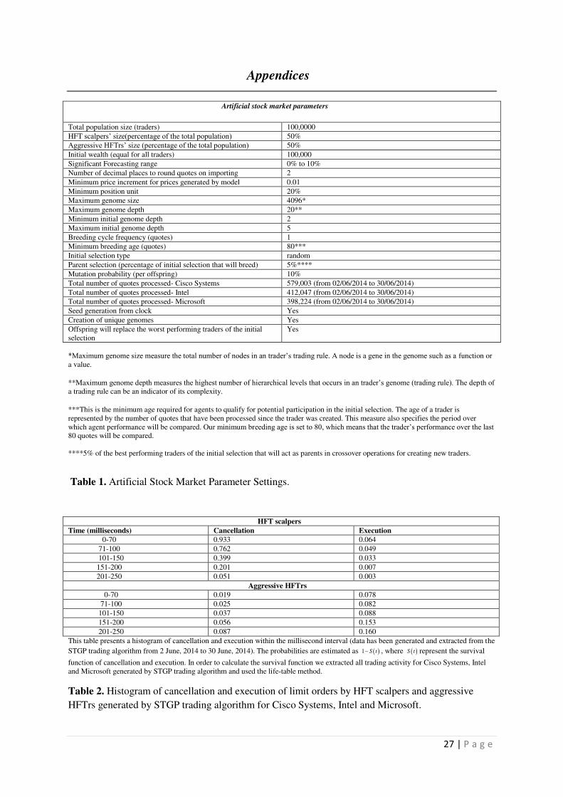
In contrast to all other studies, we are able to directly observe the number of executed and cancelled

orders by extracting generated data from the STGP trading algorithm (reported in Table 2).

Interestingly, a very large number of limit orders submitted by HFT scalpers are cancelled within a

very short interval of order submission. According to Table 2, 70Cancel

P , the probability of a

cancellation within 70 milliseconds is 0.933. By the time 250 milliseconds has elapsed, this

probability substantially decreases to 0.051. At the same time the probability of cancellation for

aggressive HFTrs measured at 70 milliseconds is 0.019 increasing to 0.087 at 250 milliseconds.

A comparison of cancelled orders by HFT scalpers and aggressive HFTrs indicates that HFT scalpers

cancel a significantly larger proportion of orders after a very short duration.

3 All trading volumes, latency arbitrage opportunities, profits and latency arbitrage costs are comparable within

artificial stock market settings.

0, t

15 | P a g e

Table 2 suggests that although HFT scalpers cancel a large number of trading orders within 70

milliseconds to position themselves at the top of the order book, between 0 and 70 milliseconds, their

execution rate is also quite high. At the same time, the aggressive HFTrs’ orders reach the market at a

later stage and the orders are executed at worse prices due to the increasing steep pricing schedule.

Lower latency demonstrated by the HFT scalpers provides them with a large number of latency

arbitrage opportunities. Moreover, HFT scalpers purchasing the three stocks that aggressive HFTrs

intend to buy could increase asset prices before aggressive HFTrs submit trading orders, thereby

increasing their costs. In real-life trading many market participants are not equipped with powerful

computers and sophisticated trading algorithms and they usually update their trading positions with

delays. During periods of delays their orders become stale and faster traders quickly capture them. Li

(2014) examines the strategic interactions of HFTs with different speeds and concludes that front-

running HFTs should impose a speed tax on normal traders, making markets less liquid and prices less

informative.

We subscribe directly to the NASDAQ SIP feed, which provides the NBBO for all stocks listed on

NASDAQ to estimate the actual latency magnitude between the two groups of artificial high

frequency traders and NASDAQ NBBO using the following equations:

( , )HFTscalpers HFTscalpers i t NBBOLatency Timestamp Timestamp (3)

( , )aggressiveHFTrs aggressiveHFTrs i t NBBOLatency Timestamp Timestamp (4)

where ,HFTscalpers i tTimestamp measure the trading messages processes by HFT scalpers directly from

the NASDAQ SIP for security i at time t , .aggressiveHFTrs i tTimestamp measures the trading message

processes by aggressive HFTrs directly from the NASDAQ SIP for security i at time t ,

NBBOTimestamp represents NASDAQ NBBO data from 2nd of June, 2014 to 30th of June, 2014.

We extract the generated data from the three artificial stock markets to compare the performance of

HFT scalpers and aggressive HFTrs with NASDAQ NBBO for the period under investigation.

16 | P a g e

Negative latency values of Equations (3) and (4) indicate that HFT scalpers and aggressive HFTrs are

able to calculate NASDAQ NBBO faster than the NASDAQ SIP. Tables 3, 4, and 5 illustrate that

while HFT scalpers generate negative latency values between 1.5 and 2.8 milliseconds, aggressive

HFTrs generate positive latency values between 1.8 and 5.2. This finding suggests that HFT scalpers

are capable of calculating NASDAQ NBBO at least 1.5 milliseconds ahead of the public NASDAQ

SIP feed for the three financial instruments. Our empirical results demonstrate that negative latency

values are associated with a number of latency arbitrage opportunities. HFT scalpers’ ability to

calculate NASDAQ NBBO between 1.5 and 2.8 milliseconds ahead of the public NASDAQ SIP

provides them with latency arbitrage opportunities. Tables 3, 4 and 5 show that the number of latency

arbitrage opportunities vary between 306 and 1,609 per day per stock.

While the SEC’s 2010 concept of equity market structure suggests that latency for the SIPs is about 5

milliseconds, the average latency of HFT scalpers for the Cisco Systems is 1.81 milliseconds,1.92

milliseconds for Intel, and 1.99 milliseconds for Microsoft. As a comparison, the average time it takes

to execute a trading order is about 300 microseconds (Ding et al., 2014). Hence, those other market

participants who are waiting for trading messages from NASDAQ NBBO in order to decide at what

price to place their trading orders for Cisco Systems, Intel and Microsoft, can face disadvantages. One

example of latency arbitrage includes dark pools that implement NASDAQ NBBO as a reference

price for matching trading orders can be matched. Assuming that NASDAQ updates Cisco Systems’

bid price from $27 to $28, and the ask price is still $29, the mid-price will change from $28 to $28.5.

In the first 1.5 to 2.8 milliseconds, slower traders such as aggressive HFTrs are not aware of the price

change and if they place trading orders at mid-price in a dark pool, faster traders such as HFT scalpers

can purchase the stock at $28. This will allow HFT scalpers to sell Cisco Systems in the dark pool for

$28.50 after 2.8 milliseconds have elapsed.

Next, we calculate the daily Herfindahl trading concentration index for NASDAQ NBBO, which

includes data from different U.S exchanges. The relatively large variation in the Herfindahl index

values reported in the last column of Tables 3, 4 and 5 suggest that the NASDAQ NBBO dataset

17 | P a g e

represent the true fragmentation of trading at the best bid and best offer collected from a number of

different trading venues.

Table 6 illustrates the correlations between HFT scalpers’ variables in the form of univariate

regressions with security fixed effects. The correlations are very useful for evaluating the implications

of latency arbitrage opportunities on stock properties. We estimate the statistical significance,

controlling for heteroskedasticity by using the following regression:

Number of latency arbitrage opportunitiesi,t= , ,i i t i tx (5)

where the number of latency opportunitiesi,t measure the latency opportunities for security i on day t ,

i represents the fixed security effect, and ,i tx is the characteristic for security i on day t . We have

taken logarithms of price, trading volume, and the number of latency opportunities in order to account

for the substantial cross-sectional heteroskedasticity of the variables.

Table 6 reports that correlations between the number of latency arbitrage opportunities, price,

volatility and trading volume are all positive and statistically significant at 0.95 and 0.99 levels of

significance. As the coefficients on volatility are positive and statistically significant for the number

of latency arbitrage opportunities, the more the prices of the three stocks change, the more often

latency arbitrage opportunities will occur.

Volatility can potentially act as another generator of latency arbitrage opportunities because it can

force liquidity providers to adjust their trading orders more frequently. Although trading volume is

positively correlated with the number of latency arbitrage opportunities, the Herfindahl trading

concentration index is negatively correlated with the number of latency arbitrage opportunities.

To further investigate the relationship between HFT scalpers’ latency arbitrage activity and NASDAQ

NBBO, we estimate pooled, fixed effect regressions of changes to price updates at two price levels

relative to the inside on changes in quote midpoint prices and quoted depth.

18 | P a g e

Our analysis is limited to two price levels because day traders usually use level two quotes to access

bids and offers for a particular financial instrument. We estimate the following model for the two

dependent variables such as a change in the quote midpoint prices and the quoted depth:

5 51 2

0 , , ,

1 1

it k i t k k i t k i t it it

k k

Y Numpriceupdates Numpriceupdates X

(6)

where itY measure changes in quote midpoint prices and quoted depth regressed on changes to price

message updates at the inside and the first price away from the inside quote for stock i at time t ,

1

,i t kNumpriceupdates and

2

,i t kNumpriceupdates represent changes in the number of price

updates for the inside quoted prices and the first and second price levels relative to the inside quotes,

X consists of a set of control variables including 10 lags of each of the two dependent variables: five

periods of lagged volume, five lags of each bid and ask quote changes, as well as bid and ask depth

changes and time dummy variables.

We follow Harris and Saad (2014) to estimate the changes in quoted midpoint prices:

5

,

1

it i k i t k it it it

k

Midprices Messages X

(7)

where Messages consists of five independent variables such as Numpriceupdates ,

Numdepthupdates , Numreserveupdates (changes in the number of nonvisible depth updates),

Totalmessageupdates (changes in every message sent), Newmessagearrivals (changes in new

messages that do not change displayed prices), X measures the same set of controlling variables as in

Equation (6).

The physical proximity to the trading venue and the technology of the trading system both contribute

to latency. Hence, we take into account the physical as well as wire distance between the NASDAQ

SIP and our processing server by implementing a separate lag adjustment. For comparison purposes,

we select the quote lag that maximizes the number of trades that execute at NASDAQ NBBO for each

19 | P a g e

stock day. In other words, for each day and each of the three stocks there is an individual lag

adjustment. Tables 7, 8 and 9 show that changes in the NASDAQ SIP quote midpoint prices at all lags

and all price levels generated by HFT scalpers’ latency arbitrage activity, are jointly and significantly

related to changes in NASDAQ NBBO for Cisco Systems, Intel and Microsoft. We also observe that

changes in quoted depth for all lags and all price levels generated by HFT scalpers’ latency arbitrage

activity are jointly and significantly related to changes in NASDAQ NBBO for each of the three

financial instruments.

These findings confirm the assumption that HFT scalpers are able to calculate NASDAQ NBBO

ahead of the NASDAQ SIP, providing them with the opportunity of latency arbitrage (this is evident

by their ability to presage the advent of midpoint price changes up to 2.8 milliseconds in advance).

Our empirical results are consistent with Narang (2010) and McInish et al. (2014) who argue that

HFT strategies are able to jump ahead of trading orders placed by other investors via Intermarket

Sweep Orders (ISOs) and thus earn substantial profits. Patterson et al. (2013) observe that HFTrs

profit by exploiting a hidden loophole in the Chicago Mercantile Exchange (CME). This loophole

allows HFTrs with a direct connection to the CME to know of their own trade executions 10

milliseconds before informing the other market participants about the trade; this enables HFTrs to

submit other orders and use this information for trading purposes ahead of the rest of the market.

By anticipating future NBBO, HFT scalpers can capitalise on cross-market disparities prior to their

reflection in the public price quote, in effect front-running incoming trading orders to earn a small but

sure profit.

20 | P a g e

4.2.High-frequency trading profitability.

We will now quantify the latency arbitrage opportunities for our HFT scalpers. Ding et al. (2014)

suggest that the average price difference between the NASDAQ SIP and the NBBOs for Intel is

$0.0107 per share. We follow Ding et al. (2014) to estimate that the average price difference for Cisco

Systems is $0.0201 per share (average share price of Cisco Systems in June 2014 multiplied by the

percentage of average arbitrage opportunities) and $0.0083 per share for Microsoft. For a more

realistic trading scenario we employ appropriate transaction costs. Narang (2013) reports that the US

Securities and Exchange Commission (SEC) impose typical round trip transaction costs of $0.003 per

share, while we employ transaction costs of $0.004 for our profit calculations. Although slightly

higher than the current standards, the level of transaction costs take into account the operational costs

of HFT companies such as investments in technology, data and collection fees, as well as salaries.

These include software platforms, labour and risk management systems but do not include the co-

location of servers. Multiplying the average price difference following transaction costs by the trading

volume of the three financial instruments reported in column 2 of Table 10 yields the profits

accumulated by HFT scalpers on each trading day for each stock. We find positive relationship

between trading volume generated by our artificial stock market traders and HFT scalpers’ profits.

The lowest risk-free profit generated by HFT scalpers was $48.49 for Microsoft on 23rd of June, 2014,

while the highest risk-free profit of $382.00 was recorded for Cisco Systems on 18th of June, 2014.

The average risk-free profit per day for trading Cisco Systems in June 2014 was $312.94; $104.42 for

trading Intel; and $61.13 for trading Microsoft. Brogaard et al. (2013) can be seen to examine 26 high

frequency trading companies trading on NASDAQ between 2008 and 2009, reporting that they earn

an average profit of $30 per day, per company for small stocks, $174 for medium and $6,651 for

large. However, the authors report substantially high trading volumes for all stocks traded by the 26

high frequency firms.

21 | P a g e

Considering the fact that that the average price difference between the NASDAQ SIP and the

NASDAQ NBBOs is $0.0201 per share for Cisco Systems, $0.0107 for Intel, and $0.0083 for

Microsoft, we calculate the cost of HFT scalpers’ latency on institutional investors submitting random

market orders. We estimate that there are 1,094 latency arbitrage opportunities for Cisco Systems on

2nd of June, 2014 during the 6.5-hour trading day (approximately 0.047 latency arbitrage opportunities

per second). Considering the latency of 1.6 milliseconds for HFT scalpers for this particular day,

implies that for 0.0752 (0.047 multiplied by 1.6) milliseconds of each second the NASDAQ SIP and

the NASDAQ NBBO differ. This could result in a buy or sell order heading to the wrong trading

exchange half that often: 0.038%. We multiply the average price difference of $0.0201 by the

percentage of the time latency arbitrage opportunities occur (0.038%), to estimate an expected latency

arbitrage opportunity of $0.00076 per 100 shares for a market order submitted randomly during

trading time. We then multiply this amount of money by Cisco Systems’ trading volume of 20,347 for

2nd of June, 2014 to find out that the cost of latency arbitrage for that day was $0.15.

Table 11 indicates that the lowest cost of HFT scalpers’ latency arbitrage on institutional traders was

$0.02 for Microsoft on 12th,16th and 19th of June and the highest latency arbitrage cost was $0.19 for

Cisco Systems on 4th and 24th of June. The average cost of latency arbitrage for Cisco systems was

$0.13; $0.04 for Intel; and $0.04 for Microsoft. Although these numbers suggest that market

participants submitting random market orders are unlikely to experience significant latency arbitrage

costs, investors trading when latency opportunities occur are facing substantial costs. This is

especially valid in real-life trading, where all HFT companies generate a huge trading volume

resulting in high levels of latency arbitrage costs. However, one of the shortcomings of our cost of

latency estimations is that NASDAQ NBBO is updated many times per second (artificial stock market

traders also submit trading orders many times per second) resulting in more than 0.047 latency

arbitrage opportunities per second.

22 | P a g e

4.3.High-frequency trading and market quality

Biais et al. (2011), Budish et al. (2013), Schwartz and Wu (2013), and Menkveld (2014) argue that

the superhuman speed of trading and a continuous limit order book could lead to a socially wasteful

arms race amongst HFTrs, imposing severe disadvantages on traditional investors. Narang (2010)

reports that the current rebate stock market structure based on volume unfairly benefits HFTrs over

ordinary traders. To test these arguments empirically we examine the implications of HFT scalpers’

latency arbitrage activity on market quality by defining several measures of market quality: two

measures of liquidity and two measures of short-term volatility . The first measure of liquidity is the

Effective Spread ((best ask price – best bid price) / (bestask + bestbid) / 2). Depth represents the

second measure of liquidity and is estimated as the time-weighted average of the number of trades in

the book at the best posted prices in the sample period. The first measure of short-term volatility (HP

– LP) is defined as the highest price minus the lowest price divided by the midpoint of the highest

price and the lowest price in the sample. High-Low represents the second measure of short-term

volatility and is defined as the highest mid-quote minus the lowest mid-quote. While HFT scalpers’

trading volume and market quality are dependent variables in our experiment, five lags of the two

dependent variables act as explanatory variables. The bivariate VAR model of HFT scalpers’ trading

volume and market quality for each day from 2nd of June, 2014 to 30th of June, 2014 has been

designed to capture the trading activity for each stock and each day in the sample:

(8)

(9)

where is the total volume for the period, and is the market quality variable.

There are four measures as a proxy for market quality: The Effective Spread, Depth, HP-LP and High-

Low.

5 5

, , , ,

1 1

i t i i i t k k i t k i t

k k

HFTscalpers a b MQ c HFTscalpers

5 5

, , , ,

1 1


k k

MQ MQ HFTscalpers

,i tHFTscalpers ,i t

MQ

23 | P a g e

The results reported in Table 12 demonstrate the negative implications of HFT scalpers’ latency

arbitrage activity on market quality. A comparison between HFT scalpers and HP- LP indicates that

HFT scalpers are significantly affected by intra-day volatility, and volatility is increased as a result of

the activity of HFT scalpers. We examine the effect of HFT scalpers on High- Low and observe that,

as with HP-LP, the volatility has an effect on HFT scalpers and HFT scalpers increase intraday

volatility. After analysing the effect of HFT scalpers on the Effective Spread and finding that the

coefficients 0.079 and (-0.003) for the first lagged HFT scalpers are insignificant, we conclude that

HFT scalpers’ activity does not significantly narrow the subsequent effective spread for the three

stocks within the artificial stock market settings. Finally, we examine the relation between HFT

scalpers and Depth and find that a higher level of HFT scalpers’ activity is associated with lower

levels of market depth. Our empirical findings show that market efficiency is negatively affected by

the trading activity of HFT scalpers, with no countervailing benefit in volatility or any other measured

variable. These findings are in line with Lee (2014) but counter to the results of Brogaard (2010),

Hansbrouck and Saar (2009) and Hendershott and Riordan (2011).

4.4 High-frequency trading and market regulation.

Trading at superhuman speeds poses potential regulatory questions, including whether such rapid

trading has negative implications on a broker’s ability to perform affirmative obligations, such as

execution at NBBO prices. Considering the fact that HFT scalpers are already much faster than other

market participants, their ability to invest in the latest software technology to shave a few

milliseconds off creates the conditions of an arms race. Our experimental results suggest that HFT

scalpers’ latency arbitrage activity precipitates an arms race, as even faster traders can calculate

NASDAQ NBBO to see the future NASDAQ NBBO, and so on. The speed race could lead to a

classic prisoner’s dilemma: HFT scalpers invest in speed to try to capture as many as possible latency

arbitrage opportunities, aggressive HFTrs should invest in speed to match HFT scalpers’ trading

activity; and all market participants should be better off if they collectively decide not to invest in

speed, but it is each market participant interest to continue to invest in speed. Similar to Budish et al.

(2013), we observe that the latency arms race is a result of continuous trading.

24 | P a g e

Budish et al. (2013) argue that the HFT arms race is a result of the continuous operation of current

financial markets and propose the introduction of frequent batch auctions. These batch auctions

represent uniform-price sealed-bid double auctions performed at frequent but also discrete time

intervals. The auction takes the form of a sealed bid not visible to other traders during the batch

interval and the exchange collects all receive orders at the end of each batch interval, estimating the

aggregate of demand and supply functions out of all bid and ask orders. The market should clear at the

point where supply equals demand, with all transactions occurring at the same price, which is the

uniform price. Trading orders are not visible to other traders and the exchange distributes the

aggregate supply and demand functions at the end of each batch interval. The authors suggest that

frequent batch auctions can eliminate the arms race by significantly reducing the value of a tiny speed

advantage. The current continuous order book process allows latency arbitrage and front-running of

trading orders due to the serial sequence of market orders. In contrast, under the conditions for batch

auctions, multiple traders observe the same information at the same time enhancing price rather than

speed competition. Budish et al. (2013) suggest that in equilibrium of the batch auctions, bid-ask

spreads are narrower and markets are deeper providing greater social welfare. Moreover, batch

auctions provide exchanges, with longer periods of time for processing orders before the next queue

of batch orders. This could ease the computational process in all trading venues world-wide, making

financial markets less vulnerable to crises like the Flash Crash in 2010. The authors propose batch

auctions at intervals such as once per second (23,400 times per day per security). Although, Menkveld

(2014) claims that batch auctions should be scheduled at a rate of 10 auctions per second, enabling

traders to see the prices in the last auction before conducting the next auction, our empirical results

illustrate that HFT scalpers generate large profits and cancel a large number of orders in very short

intervals, that is, between 0 and 70 milliseconds (reported in Table 2). Introducing batch auctions at

frequencies such as 10 per second could prove inefficient, so, we therefore recommend the

implementation of batch auctions once per 70 milliseconds (334,285 times per 6.5 – hour trading day

per security) based on the distribution of cancelled orders in Table 2. Bunching together incoming

trading orders every 70 milliseconds would impose a queuing risk for HFT scalpers, leading to

positive implications for market quality.

25 | P a g e

5.Conclusions

The application of sophisticated computational trading strategies at very low latency has increased

over time. Significant trading software improvements are constantly introduced, raising operating

costs and increasing competitive advantage among market participants. As communication and

trading speed in financial markets has decreased over time, regulators face additional challenges in

terms of addressing the speed differentials of market participants.

In this study, we simulate real-life trading within artificial stock market settings and observe that HFT

scalpers are able to calculate NASDAQ NBBO at least 1.5 milliseconds ahead of the NASDAQ SIP,

creating a large number of latency arbitrage opportunities. We also measure the precise level of

profits generated by HFT scalpers and the exact costs of latency arbitrage to other market participants.

Moreover, we observe that HFT scalpers’ latency arbitrage activity accumulates a large number of

cancelled orders in a very short period of time, which may make trading more difficult and costly for

traditional investors who lack access to sophisticated trading platforms. If one group of market

participants such as HFT scalpers is able to calculate NASDAQ NBBO ahead of the NASDAQ SIP,

those participants with lower latency would have an unfair advantage in the marketplace creating

socially wasteful arms race for speed. We observe that the size of the arbitrage opportunity, and hence

the harm to traditional investors, may depend on the magnitude of speed and the cost of cutting-edge

speed improvements.

In terms of market quality, we have found that HFT scalpers’ latency arbitrage activity has negative

implications on market efficiency, as intraday volatility increases and market depth decreases.

Nearly all financial markets around the world operate on a continuous trading basis, allowing

computationally advantaged traders such as HFT scalpers to generate risk-free profits. We propose an

alternative financial market mechanism such as the batch auctioned market, which successfully

eliminates latency arbitrage opportunities and improves efficiency. A batch auctioned financial

market could prevent HFTrs from gaining an advantage in terms of latency, thereby increasing surplus

for ordinary traders.

26 | P a g e

We suggest the implementation of batch auctions once in every 70 milliseconds, that is 334,285 times

per 6.5-hour trading day per financial instrument. If trading orders are bunched together every 70

milliseconds, HFT scalpers could face a queuing risk, leading to a less harmful market quality effect.

Perhaps the main practical implication of our study comes from our demonstrating that market

regulators and operators can apply artificial intelligence tools such as STGP to conduct trading

behaviour-based profiling, as well as capture the occurrence of new HFT strategies and examine their

impact on the financial markets. However, a possible limitation of this study is that all trading

volumes, latency arbitrage opportunities, profits and latency arbitrage costs are comparable within

artificial stock market settings. In comparison with real-life investors, artificial traders are

programmed to obey orders and perform certain tasks lacking feelings and emotions. In any case,

trading at superhuman speeds is likely to remain a major field of interest for researchers as well as a

concern for market regulators over the next few years.

27 | P a g e

Appendices

Artificial stock market parameters

Total population size (traders) 100,0000

HFT scalpers’ size(percentage of the total population) 50%

Aggressive HFTrs’ size (percentage of the total population) 50%

Initial wealth (equal for all traders) 100,000

Significant Forecasting range 0% to 10%

Number of decimal places to round quotes on importing 2

Minimum price increment for prices generated by model 0.01

Minimum position unit 20%

Maximum genome size 4096*

Maximum genome depth 20**

Minimum initial genome depth 2

Maximum initial genome depth 5

Breeding cycle frequency (quotes) 1

Minimum breeding age (quotes) 80***

Initial selection type random

Parent selection (percentage of initial selection that will breed) 5%****

Mutation probability (per offspring) 10%

Total number of quotes processed- Cisco Systems 579,003 (from 02/06/2014 to 30/06/2014)

Total number of quotes processed- Intel 412,047 (from 02/06/2014 to 30/06/2014)

Total number of quotes processed- Microsoft 398,224 (from 02/06/2014 to 30/06/2014)

Seed generation from clock Yes

Creation of unique genomes Yes

Offspring will replace the worst performing traders of the initial selection

Yes

*Maximum genome size measure the total number of nodes in an trader’s trading rule. A node is a gene in the genome such as a function or a value.

**Maximum genome depth measures the highest number of hierarchical levels that occurs in an trader’s genome (trading rule). The depth of a trading rule can be an indicator of its complexity.

***This is the minimum age required for agents to qualify for potential participation in the initial selection. The age of a trader is represented by the number of quotes that have been processed since the trader was created. This measure also specifies the period over which agent performance will be compared. Our minimum breeding age is set to 80, which means that the trader’s performance over the last 80 quotes will be compared. ****5% of the best performing traders of the initial selection that will act as parents in crossover operations for creating new traders.

Table 1. Artificial Stock Market Parameter Settings.

HFT scalpers

Time (milliseconds) Cancellation Execution

0-70 0.933 0.064

71-100 0.762 0.049

101-150 0.399 0.033

151-200 0.201 0.007

201-250 0.051 0.003

Aggressive HFTrs

0-70 0.019 0.078

71-100 0.025 0.082

101-150 0.037 0.088

151-200 0.056 0.153

201-250 0.087 0.160

This table presents a histogram of cancellation and execution within the millisecond interval (data has been generated and extracted from the

STGP trading algorithm from 2 June, 2014 to 30 June, 2014). The probabilities are estimated as 1 S t , where S t represent the survival

function of cancellation and execution. In order to calculate the survival function we extracted all trading activity for Cisco Systems, Intel and Microsoft generated by STGP trading algorithm and used the life-table method.

Table 2. Histogram of cancellation and execution of limit orders by HFT scalpers and aggressive

HFTrs generated by STGP trading algorithm for Cisco Systems, Intel and Microsoft.

28 | P a g e

HFT scalpers

Date Trading volume Latency* Number of latency

arbitrage

opportunities

Herfindahl index for

NASDAQ NBBO

02/06/2014 20,347 -1.6 1094 3.86

03/06/2014 19,009 -1.5 1502 4.92

04/06/2014 19,822 -1.5 1500 4.93

05/06/2014 18,251 -1.8 912 2.81

06/06/2014 18,111 -1.6 1000 3.87

09/06/2014 15,983 -1.9 803 2.72

10/06/2014 22,575 -2.0 687 2.54

11/06/2014 20,262 -2.1 610 1.50

12/06/2014 19,999 -2.1 608 1.51

13/06/2014 19,634 -2.0 699 2.48

16/06/2014 19,120 -2.2 517 1.46

17/06/2014 17,845 -1.8 900 3.83

18/06/2014 23,727 -1.6 1036 4.88

19/06/2014 16,891 -1.7 1001 4.79

20/06/2014 18,776 -2.0 690 2.51

23/06/2014 20,292 -2.4 477 2.45

24/06/2014 19,890 -1.5 1511 4.94

25/06/2014 18,276 -1.6 1029 4.86

26/06/2014 18,393 -1.5 1517 4.95

27/06/2014 20,818 -1.9 800 3.74

30/06/2014 20,164 -1.8 911 3.80

Aggressive HFTrs

02/06/2014 7,557 2.8 0 1.29

03/06/2014 8,313 3.3 0 1.31

04/06/2014 8,001 3.0 0 1.43

05/06/2014 9,123 3.5 0 1.38

06/06/2014 9,204 2.0 0 1.24

09/06/2014 11,782 2.5 0 2.31

10/06/2014 4,882 2.8 0 0.99

11/06/2014 6,999 2.7 0 0.84

12/06/2014 7,524 2.9 0 1.27

13/06/2014 8,009 3.0 0 1.26

16/06/2014 8,110 3.1 0 1.43

17/06/2014 10,030 2.6 0 1.32

18/06/2014 3,626 2.3 0 0.19

19/06/2014 10,889 2.2 0 1.85

20/06/2014 6,856 2.0 0 1.20

23/06/2014 6,161 2.1 0 1.19

24/06/2014 8,251 2.2 0 1.48

25/06/2014 9,552 2.7 0 0.90

26/06/2014 9,774 2.5 0 0.85

27/06/2014 6,984 3.0 0 2.29

30/06/2014 7,006 2.7 0 1.37 This table presents the trading volume, the latency, the number of latency opportunities and the Herfindahl index for Cisco Systems from 2nd of June, 2014 to 30th of June, 2014 generated by STGP.

* We estimate the actual latency magnitude between the two groups of artificial high frequency traders and NASDAQ NBBO using the following equations:

( , )HFTscalpers HFTscalpers i t NBBO

Latency Timestamp Timestamp

( , )aggressiveHFTrs aggressiveHFTrs i t NBBO


Negative latency values indicates that HFT scalpers and aggressive HFTrs are able to calculate NASDAQ NBBO faster than NASDAQ SIP.

Table 3. Statistical measures for Cisco Systems from 2nd of June, 2014 to 30th of June, 2014 generated by HFT scalpers and aggressive HFTrs.

29 | P a g e

HFT scalpers


arbitrage

opportunities


NASDAQ NBBO

02/06/2014 13,237 -2.0 619 2.62

03/06/2014 14,002 -1.9 778 3.74

04/06/2014 15,265 -2.2 501 2.57

05/06/2014 15,789 -2.5 388 1.51

06/06/2014 16,489 -1.9 723 2.83

09/06/2014 12,983 -1.6 937 3.89

10/06/2014 13,671 -1.9 774 3.80

11/06/2014 14,189 -1.5 1099 4.97

12/06/2014 15,126 -2.4 380 1.50

13/06/2014 14,172 -2.2 511 2.56

16/06/2014 16,818 -2.5 373 1.49

17/06/2014 14,767 -1.8 905 3.89

18/06/2014 13,120 -1.7 897 3.90

19/06/2014 13,888 -1.7 1000 4.90

20/06/2014 12,119 -1.5 1507 4.99

23/06/2014 14,662 -1.6 1015 4.92

24/06/2014 13,000 -2.3 571 3.66

25/06/2014 12,981 -2.2 638 3.63

26/06/2014 15,126 -2.1 777 2.01

27/06/2014 14,220 -1.7 923 3.88

30/06/2014 14,003 -1.5 1609 4.96

Aggressive HFTrs

02/06/2014 6,771 3.9 0 1.23

03/06/2014 5,877 4.2 0 1.20

04/06/2014 3,266 4.0 0 1.28

05/06/2014 3,115 2.7 0 1.34

06/06/2014 2,107 2.9 0 1.33

09/06/2014 6,270 3.1 0 0.89

10/06/2014 6,145 3.2 0 1.03

11/06/2014 5,001 2.5 0 0.49

12/06/2014 3,999 2.8 0 1.77

13/06/2014 4,148 3.0 0 1.49

16/06/2014 2,288 5.2 0 0.78

17/06/2014 4,115 3.3 0 1.30

18/06/2014 5,772 1.9 0 1.76

19/06/2014 5,509 2.4 0 1.29

20/06/2014 6,004 3.7 0 2.25

23/06/2014 4,778 2.1 0 2.24

24/06/2014 6,717 1.8 0 1.22

25/06/2014 6,992 3.5 0 2.38

26/06/2014 4,116 2.6 0 1.44

27/06/2014 5,124 2.0 0 2.41

30/06/2014 5,233 2.3 0 1.39 This table presents the trading volume, the latency, the number of latency opportunities and the Herfindahl index for Intel from 2nd of June, 2014 to 30th of June, 2014 generated by STGP.

* We estimate the actual latency magnitude between the two groups of artificial high frequency traders and NASDAQ NBBO using the following equations:






Table 4. Statistical measures for Intel from 2nd of June, 2014 to 30th of June, 2014 generated by HFT scalpers and aggressive HFTrs.

30 | P a g e

HFT scalpers


arbitrage

opportunities


NASDAQ NBBO

02/06/2014 14,237 -1.9 781 3.82

03/06/2014 15,944 -1.9 779 3.81

04/06/2014 15,161 -2.1 733 3.69

05/06/2014 16,120 -1.7 845 2.70

06/06/2014 14,266 -1.5 1500 4.99

09/06/2014 13,353 -1.5 1514 4.98

10/06/2014 12,348 -1.7 874 3.71

11/06/2014 14,003 -1.8 912 3.63

12/06/2014 16,272 -2.7 327 2.55

13/06/2014 16,400 -2.5 410 2.59

16/06/2014 13,445 -2.8 306 1.54

17/06/2014 14,894 -2.0 732 3.78

18/06/2014 14,122 -2.1 719 3.63

19/06/2014 13,009 -2.5 403 2.59

20/06/2014 12,474 -1.8 838 3.62

23/06/2014 11,277 -1.9 700 2.88

24/06/2014 14,820 -1.5 1508 4.94

25/06/2014 13,995 -1.7 936 4.90

26/06/2014 13,823 -2.1 699 2.53

27/06/2014 14,237 -2.2 642 2.61

30/06/2014 14,336 -2.0 863 3.77

Aggressive HFTrs

02/06/2014 4,002 2.6 0 1.33

03/06/2014 3,888 3.1 0 1.29

04/06/2014 3,997 3.4 0 1.26

05/06/2014 3,555 3.0 0 0.93

06/06/2014 4,111 2.7 0 0.99

09/06/2014 5,373 2.9 0 1.30

10/06/2014 6,661 2.3 0 1.35

11/06/2014 5,822 2.0 0 2.36

12/06/2014 3,119 3.7 0 2.27

13/06/2014 3,005 3.5 0 1.28

16/06/2014 5,474 2.8 0 1.32

17/06/2014 4,585 2.6 0 1.34

18/06/2014 4,778 2.2 0 2.29

19/06/2014 5,116 2.1 0 1.33

20/06/2014 6,828 2.1 0 1.30

23/06/2014 7,080 1.9 0 2.41

24/06/2014 4,821 2.5 0 1.28

25/06/2014 5,112 2.4 0 1.27

26/06/2014 5,228 2.5 0 1.34

27/06/2014 4,999 2.3 0 1.35

30/06/2014 5,021 2.5 0 0.87 This table presents the trading volume, the latency, the number of latency opportunities and the Herfindahl index for Microsoft from 2nd of June, 2014 to 30th of June, 2014 generated by STGP.

* We measure the latency by estimating the amount of time between the HFT scalpers and aggressive HFTrs time stamps at SIP and the NBBO as follows:






Table 5. Statistical measures for Microsoft from 2nd of June, 2014 to 30th of June, 2014 generated by HFT scalpers and aggressive HFTrs.

31 | P a g e

Cisco Systems

Statistical measure Log (price) Log (trading

volume)

Volatility Herfindahl index

Log (number of

latency arbitrage

opportunities)

1.75* 0.52* 21.36** -3.27**

Intel

Log (number of

latency arbitrage

opportunities)

1.36** 0.61* 17.88** -2.91**

Microsoft

Log (number of

latency arbitrage

opportunities)

1.93** 0.66* 15.91** -3.01**

This table shows the statistical significance between HFT scalpers’ variables generated by STGP from 2nd of June, 2014 to 3oth of June, 2014. Regressions are performed for each measure of the number of latency opportunities for each independent variable, and therefore the table reports coefficients for 12 regressions in total. Each regression accommodate security fixed effects. Volatility is measured as percentage difference between the day’s highest and lowest prices. Statistical significance has been calculated controlling for heteroskedasticity:

Number of latency arbitrage opportunities i,t = , ,i i t i tx ,

where number of latency opportunities i,t measures the latency opportunities for security i on day t , i

represents the fixed security effect

and ,i t

x is the characteristic for security i on day t.

*Indicates statistical significance at 0.99 level. **Indicates statistical significance at 0.95 level.

Table 6. Correlations between HFT scalpers’ variables generated by STGP form 2nd of June, 2014 to 30th of June, 2014.

Dependent variable Change in quote midpoint prices Change in quoted depth 1

1tNumpriceupdates 0.028* 0.041**

1

2tNumpriceupdates 0.021** 0.019**

1

3tNumpriceupdates 0.062* 0.010*

1

4tNumpriceupdates 0.024* 0.007*

1

5tNumpriceupdates 0.038** 0.006*

2


2


2


2

4tNumpriceupdates 0.188** 0.479*

2


Adjusted R2 0.22 0.39 This table consist of pooled, fixed effects, regressions for Cisco Systems estimated by jointly examining the relationship between the change in the number of price updates segmented by the relative proximity to the best posted quotes on subsequent changes in quote midpoint prices and quoted depth for the stock. We estimate the following model for the two dependent variables such as change in quote midpoints and quoted depth:

5 51 2

0 , , ,

1 1


k k


where itY measure changes in quote midpoint prices and quoted depth regressed on changes to price message updates at the inside and

the first price away from the inside quote for stock i at time t , 1

,i t kNumpriceupdates and 2

,i t kNumpriceupdates

represent changes in the number of price updates at the inside quoted prices and the first and second price levels relative to the inside quotes,

X consists of a set of control variables including 10 lags of each of the two dependent variables; five periods of lagged volume; five lags of each of bid and ask quote changes as well as bid and ask depth changes; and time dummy variables. All coefficients in the table have been multiplied by 10. *Indicates statistical significance at 0.99 level. **Indicates statistical significance at 0.95 level.

Table 7. The relationship between HFT scalpers’ latency arbitrage activity and NASDAQ NBBO for Cisco Systems.

32 | P a g e

Dependent variable Change in quote midpoint prices Change in quoted depth

1

1tNumpriceupdates

0.019** 0.057*

1

2tNumpriceupdates

0.012** 0.049*

1

3tNumpriceupdates

0.044** 0.035*

1

4tNumpriceupdates

0.035* 0.018**

1

5tNumpriceupdates

0.030** 0.009**

2

1tNumpriceupdates

0.411** 0.403*

2

2tNumpriceupdates

0.236** 0.448*

2

3tNumpriceupdates

0.115* 0.399*

2

4tNumpriceupdates

0.253** 0.476*

2

5tNumpriceupdates

0.286** 0.290**

Adjusted R2 0.19 0.27

This table consist of pooled, fixed effects, regressions for Intel estimated by jointly examining the relationship between the change in the number of price updates segmented by the relative proximity to the best posted quotes on subsequent changes in quote midpoint prices and quoted depth for the stock. We estimate the following model for the two dependent variables such as change in quote midpoints and quoted depth: 5 5

1 2

0 , , ,

1 1


k k








Table 8. The relationship between HFT scalpers’ latency arbitrage activity and NASDAQ NBBO for Intel.

Dependent variable Change in quote midpoint prices Change in quoted depth

1

1tNumpriceupdates

0.020* 0.074**

1

2tNumpriceupdates

0.013* 0.048*

1

3tNumpriceupdates

0.032** 0.033*

1

4tNumpriceupdates

0.031** 0.015**

1

5tNumpriceupdates

0.045** 0.0010*

2

1tNumpriceupdates

0.119* 0.447*

2

2tNumpriceupdates

0.203** 0.406*

2

3tNumpriceupdates

0.284** 0.428**

2

4tNumpriceupdates

0.267** 0.399**

2

5tNumpriceupdates

0.217* 0.306**

Adjusted R2 0.27 0.49

This table consist of pooled, fixed effects, regressions for Microsoft estimated by jointly examining the relationship between the change in the number of price updates segmented by the relative proximity to the best posted quotes on subsequent changes in quote midpoint prices and quoted depth for the stock. We estimate the following model for the two dependent variables such as change in quote midpoints and quoted depth: 5 5

1 2

0 , , ,

1 1


k k








Table 9. The relationship between HFT scalpers’ latency arbitrage activity and NASDAQ NBBO for Microsoft.

33 | P a g e

Cisco Systems

Date Trading volume (shares)* Average price difference** Profits

02/06/2014 20,347 0.0161 $327.59

03/06/2014 19,009 0.0161 $306.04

04/06/2014 19,822 0.0161 $319.13

05/06/2014 18,251 0.0161 $293.84

06/06/2014 18,111 0.0161 $291.59

09/06/2014 15,983 0.0161 $257.33

10/06/2014 22,575 0.0161 $363.45

11/06/2014 20,262 0.0161 $326.22

12/06/2014 19,999 0.0161 $321.98

13/06/2014 19,634 0.0161 $316.10

16/06/2014 19,120 0.0161 $307.83

17/06/2014 17,845 0.0161 $287.30

18/06/2014 23,727 0.0161 $382.00

19/06/2014 16,891 0.0161 $271.94

20/06/2014 18,776 0.0161 $302.29

23/06/2014 20,292 0.0161 $326.70

24/06/2014 19,890 0.0161 $320.22

25/06/2014 18,276 0.0161 $294.24

26/06/2014 18,393 0.0161 $296.12

27/06/2014 20,818 0.0161 $335.17

30/06/2014 20,164 0.0161 $324.64

Intel

02/06/2014 13,237 0.0067 $88.69

03/06/2014 14,002 0.0067 $93.81

04/06/2014 15,265 0.0067 $102.27

05/06/2014 15,789 0.0067 $105.79

06/06/2014 16,489 0.0067 $110.48

09/06/2014 12,983 0.0067 $86.99

10/06/2014 13,671 0.0067 $91.59

11/06/2014 14,189 0.0067 $95.07

12/06/2014 15,126 0.0067 $101.34

13/06/2014 14,172 0.0067 $94.95

16/06/2014 16,818 0.0067 $112.68

17/06/2014 14,767 0.0067 $98.94

18/06/2014 13,120 0.0067 $87.90

19/06/2014 13,888 0.0067 $93.05

20/06/2014 12,119 0.0067 $81.20

23/06/2014 14,662 0.0067 $98.23

24/06/2014 13,000 0.0067 $87.10

25/06/2014 12,981 0.0067 $86.98

26/06/2014 15,126 0.0067 $101.34

27/06/2014 14,220 0.0067 $95.27

30/06/2014 14,003 0.0067 $93.82

Microsoft

02/06/2014 14,237 0.0043 $61.22

03/06/2014 15,994 0.0043 $68.56

04/06/2014 15,161 0.0043 $65.19

05/06/2014 16,120 0.0043 $69.32

06/06/2014 14,266 0.0043 $61.34

09/06/2014 13,353 0.0043 $57.42

10/06/2014 12,348 0.0043 $53.10

11/06/2014 14,003 0.0043 $60.21

12/06/2014 16,272 0.0043 $69.97

13/06/2014 16,400 0.0043 $70.52

16/06/2014 13,445 0.0043 $57.81

17/06/2014 14,894 0.0043 $64.04

18/06/2014 14,122 0.0043 $60.72

19/06/2014 13,009 0.0043 $55.94

20/06/2014 12,474 0.0043 $53.63

23/06/2014 11,277 0.0043 $48.49

24/06/2014 14,820 0.0043 $63.73

25/06/2014 13,995 0.0043 $60.18

26/06/2014 13,823 0.0043 $59.44

27/06/2014 14,237 0.0043 $61.22

30/06/2014 14,336 0.0043 $61.64

*All trading volumes are generated by artificial stock market traders during real-time trading. **Measures the average price difference between NASDAQ SIP and NASDAQ NBBO after transaction costs of $0.004 per share.

Table 10. HFT scalpers’ profitability for Cisco Systems, Intel and Microsoft.

34 | P a g e

Cisco Systems

Date Trading volume

(shares)*

Number of latency

arbitrage opportunities

Latency Cost of latency

arbitrage**

02/06/2014 20,347 1,094 1.6 $0.15

03/06/2014 19,009 1,502 1.5 $0.18

04/06/2014 19,822 1,500 1.5 $0.19

05/06/2014 18,251 912 1.8 $0.13

06/06/2014 18,111 1,000 1.6 $0.12

09/06/2014 15,983 803 1.9 $0.10

10/06/2014 22,575 678 2.0 $0.13

11/06/2014 20,262 610 2.1 $0.11

12/06/2014 19,999 608 2.1 $0.11

13/06/2014 19,634 699 2.0 $0.12

16/06/2014 19,120 517 2.2 $0.09

17/06/2014 17,845 900 1.8 $0.12

18/06/2014 23,727 1,036 1.6 $0.16

19/06/2014 16,891 1,001 1.7 $0.12

20/06/2014 18,776 690 2.0 $0.11

23/06/2014 20,292 477 2.4 $0.10

24/06/2014 19,890 1,511 1.5 $0.19

25/06/2014 18,276 1,029 1.6 $0.13

26/06/2014 18,393 1,517 1.5 $0.18

27/06/2014 20,818 800 1.9 $0.13

30/06/2014 20,164 911 1.8 $0.14

Intel

02/06/2014 13,237 619 2.0 $0.04

03/06/2014 14,002 778 1.9 $0.05

04/06/2014 15,265 501 2.2 $0.04

05/06/2014 15,789 388 2.5 $0.03

06/06/2014 16,489 723 1.9 $0.05

09/06/2014 12,983 937 1.6 $0.04

10/06/2014 13,671 774 1.9 $0.04

11/06/2014 14,189 1,099 1.5 $0.05

12/06/2014 15,126 380 2.4 $0.03

13/06/2014 14,172 511 2.2 $0.04

16/06/2014 16,818 373 2.5 $0.03

17/06/2014 14,767 905 1.8 $0.05

18/06/2014 13,120 897 1.7 $0.04

19/06/2014 13,888 1,000 1.7 $0.05

20/06/2014 12,119 1,507 1.5 $0.06

23/06/2014 14,662 1,015 1.6 $0.05

24/06/2014 13,000 571 2.3 $0.04

25/06/2014 12,981 638 2.2 $0.04

26/06/2014 15,126 777 2.1 $0.06

27/06/2014 14,220 923 1.7 $0.05

30/06/2014 14,003 1,609 1.5 $0.08

Microsoft

02/06/2014 14,237 781 1.9 $0.04

03/06/2014 15,944 779 1.9 $0.04

04/06/2014 15,161 733 2.1 $0.04

05/06/2014 16,120 845 1.7 $0.04

06/06/2014 14,266 1,500 1.5 $0.06

09/06/2014 13,353 1,514 1.5 $0.05

10/06/2014 12,348 874 1.7 $0.03

11/06/2014 14,003 912 1.8 $0.04

12/06/2014 16,272 327 2.7 $0.02

13/06/2014 16,400 410 2.5 $0.03

16/06/2014 13,445 306 2.8 $0.02

17/06/2014 14,894 732 2.0 $0.04

18/06/2014 14,122 719 2.1 $0.04

19/06/2014 13,009 403 2.5 $0.02

20/06/2014 12,474 838 1.8 $0.03

23/06/2014 11,277 700 1.9 $0.03

24/06/2014 14,820 1,508 1.5 $0.06

25/06/2014 13,995 936 1.7 $0.04

26/06/2014 13,823 699 2.1 $0.03

27/06/2014 14,237 642 2.2 $0.03

30/06/2014 14,336 863 2.0 $0.04

*All trading volumes are generated by artificial stock market traders during real-time trading. **Measure the cost of HFT scalpers’ latency arbitrage on institutional traders within artificial stock market settings.

Table 11. Estimated cost of HFT scalpers’ latency arbitrage on institutional traders.

35 | P a g e

Type HFTscalperst-1 MQt-1

HFTscalpers 0.208* 0.549*

HP – LP 0.003* 0.225*

HFTscalpers 0.471* 0.079

The effective spread 0.002* -0.003


High – Low 0.647* 0.170*


Depth -0.168* -0.118*

The table reports the results of the bivariate VAR model:

5 5

, , , ,

1 1


k k

HFTscalpers a b MQ c HFTscalpers

5 5

, , , ,

1 1


k k

MQ MQ HFTscalpers

There are four different measures of market quality – two of them are related to short – term volatility (HP – LP and High – Low) and the other two are related to liquidity (The effective spread and Depth). HP – LP has been estimated as the highest price of the three financial instruments minus the lowest price divided by the midpoint of the highest price and the lowest price in the sample period (02/01/2014 – 30/06/2014). High – Low has been calculated as the highest mid – quote minus the lowest mid – quote. The effective spread is measured as ((best ask price – best bid price) / (bestask – bestbid) / 2) in the sample period. Depth represents the time – weighted average of the number of traders in the book at the best posted prices. *indicates significance at 0.99% level.

Table 12. HFT scalpers’ latency arbitrage activity generated by STGP trading algorithm for Cisco Systems, Intel and Microsoft and its implications on market quality.

36 | P a g e

References

Baron,M.,Brogaard,J.,Kirilenko,A.(2012).The trading prifits of high-frequency traders, Working paper.

Bhupathi,T.L.(2010).Technology’s latest market manipulator-High frequency trading:The strategies, tools, risks and, responses. North Carolina Journal of Law and Technology,11:477-500.

Biais,B.,Foucault,T.,Moinas,S.(2011).Equilibrium high frequency trading. International Conference of the French Finance Association (AFFI).

Bodek,H.(2013).The problem of HFT. Collected writings on high frequency trading and stock market structure

reform. Decimus Capital Markets, LLC.

Brogaard,J.(2010).High frequency trading and market quality. Working paper.

Brogaard,J.,Hendershott,T.,Riordan,R.(2013).High frequency trading and price discovery. The Review of

Financial Studies, 27(8): 2267-2306.

Brogaard,J.,Hendershott,T.,Hunt,S.,Ysusi,C.(2014).High frequency trading and the execution costs of institutional investors. The Financial Review, 49(2): 345-369.

Budish,E.,Crampton,P.,Shim,J.(2013).High frequency trading arms race: Frequent batch auctions as a market design response. Available from http://faculty.chicagobooth.edu/eric.budish/research/hft-frequentbatchauctions.pdf . Accessed on 01/05/2014.

Cohen,S.N.,Szpruch,L.(2012).A limit order book model for latency arbitrage.Mathematical Financial

Economics,6:211-227.

Ding,S.,Hanna,J.,Hendershott,T.(2014).How slow is the NBBO? A comparison with direct exchange feeds. The

Financial Review, 49(2): 313-332.

Easley,D.,O’Hara,M.,Yang,L.(2012).Differential access to price information in financial markets. Working paper.

Easley,D.,Hendershott,T.,Ramadorai,T.(2014).Levelling the trading field. Journal of Financial Markets,17:65-93.

Egginton,J.,Van Ness,B.F.,Van Ness,R.A.(2012).Quote stuffing. Working paper.

Felker,T.,Mazalov,V.,Watt,S.M.(2014).Distance-based high-frequency trading. Procedia Computer Science, 29: 2055-2064.

Foucault,T.,Hombert,J.,Rosu,I.(2013).News trading and speed. Working paper.

Friedman,D.(1993).The double auction market institution: A survey.In Friedman and Rust (editors). The double auction market: Institutions, theories, and evidence.Addison-Wesley,3-25.

Goldstein,M.A.,Kumar,P.,Graves,F.C.(2014).Computerized and high-frequency trading. The Financial Review, 49(2): 177-202.

Hasbrouck,J.,Saar,G.(2009).Technology and liquidity provision: The blurring of traditional definitions. Journal

of Financial Markets, 12: 143-172.

Harris,J.,Saad,M.(2014).The sound of silence.The Financial Review,49:203-230.

Hendershott,T.,Jones,C.M.,Menkveld,A.(2011).Does algorithmic trading improve liquidity? Journal of Finance, 66(1): 1-33.

Hendershott,T.,Riordan,R.(2011). High frequency trading and price discovery. Working paper.

Hendershott,T.,Riordan,R.(2013).Algorithmic trading and the market for liquidity. Journal of Financial and

Quantitative Analysis, 48(4): 1001-1024.

http://faculty.chicagobooth.edu/eric.budish/research/hft-frequentbatchauctions.pdf

http://faculty.chicagobooth.edu/eric.budish/research/hft-frequentbatchauctions.pdf

37 | P a g e

Hirschey,N.(2013).Do high frequency traders anticipate buying and selling pressure? Working paper.

Hirshleifer,A.,Subrahmanyam,Titman,S.(1994).Security analysis and trading patterns when some investors receive information before others. Journal of Finance,49:1665-1698.

Li,W.(2014).High frequency trading with speed hierarchies. Working paper.

Manahov.V.,Hunson,R.,Gebka.,(2014).Does high frequency trading affect technical analysis and market efficiency? And if so, how? Journal of International Financial Markets, Institutions and Money, 28: 131-157.

Menkveld,A.J.(2014).High frequency traders and market structure. The Financial Review, 49 (2): 333-344.

McInish,T.H.,Upson,J.(2013).The quote exception rule: Giving high frequency traders an unintended advantage. Financial Management, 481-501.

McInish,T.H.,Upson,J.,Wood,R.(2014).The Flash Crash: Trading aggressiveness, liquidity supply, and the impact of Intermarket Sweep Orders, The Financial Review,49(3):481-509.

Narang,M.(2010).Tradeworx,Inc.Public Commentary on SEC Market Structure Concept Release, SEC Comment letter [online]. Available from http://sec.gov/comments/s7-02-10/s70210-129.pdf Accessed on 22 of January, 2015.

Narang,R.K.(2013).Inside the black box.A simple guide to quantitative and high frequency trading. John Wiley & Sons, Inc.

Patterson,S.(2012).Dark pools. The rise of A.I. trading machines and the looming threat to Wall Street. Random House Business Books, UK.

Patterson,S.,Strasburg,J.,Pleven,L.(2013).High-speed traders exploit loophole. The Wall Street Journal. Available from: http://online.wsj.com/news/articles/SB10001424127887323798104578455032466082920 . Accessed on 11/05/2014.

Picardo,E.(2014).Top stocks high-frequency traders (HFTrs) pick [online]. Available from http://www.investopedia.com/articles/active-trading/053010/top-stocks-high-frequency-traders-hfts-pick.asp Accessed on 2nd of January, 2015.

Ready,M.(1999).The specialist’s discretion: Stopped orders and price improvement. Review of Financial

Studies,12:1075-1112.

Schneider,D.(2012).The microsecond market.IEEE Spectrum:66-81.

Schwartz,R.,Wu,L.(2013).Equity trading in the fast lane: The Staccato Alternative. Journal of Portfolio

Management,forthcoming.

Stoll,H.R.,Schenzler,C.(2006).Trades outside the quotes: Reporting delay, trading option or trade size? Journal

of Financial Economics, 79:615-653.

Van Ness,B.,Van Ness,R.,Watson,E.D.(2014).Cancelling liquidity. Working paper.

Viljoen,T.Westerholm,P.J.Zheng,H.(2014).Algorithmic trading, liquidity and price discovery: An intraday analysis of the SPI 200 futures. The Financial Review,49(2):245-270.

Wah,E.,Wellman,M.(2013).Latency arbitrage, market fragmentation, and efficiency: A two-market model.Working paper.

Wissner-Gross,A.D.,Freer,C.F.(2010).Relativistic statistical arbitrage. Physical Review E, 82:056104-1:056104-7.

Witkam, J. (2014) Altreva Adaptive Modeller, User’s Guide. Available from http://altreva.com/Adaptive_Modeler_Users_Guide.htm. Accessed on 20/01/2015.

http://sec.gov/comments/s7-02-10/s70210-129.pdf

http://online.wsj.com/news/articles/SB10001424127887323798104578455032466082920%20.%20Accessed%20on%2011/05/2014

http://online.wsj.com/news/articles/SB10001424127887323798104578455032466082920%20.%20Accessed%20on%2011/05/2014

http://www.investopedia.com/articles/active-trading/053010/top-stocks-high-frequency-traders-hfts-pick.asp

http://altreva.com/Adaptive_Modeler_Users_Guide.htm

38 | P a g e

Appendix A

Genetic Programming

The process of Genetic Programming (GP) is divided into two sub-processes: the first is the initialisation

process which generates an initial population of trading rules in a random manner, while the other sub-process is

the dynamics process which works in a similar way to Genetic Algorithms (GA). Both GA and GP comply with

the rules of Darwinian selection, crossover and mutation. However, there is a significant difference between GA

and GP where the GA population is composed of fixed-length binary strings and the population of GP is

composed of trading rules. Each trading rule in GP is written in LISP S-Expression and represented by a parse

tree. By determining both the terminal and the functional sets, each trading rule can be written in LISP S-

Expression such as:

(10)

where the terminal set is represented by , where is a constant; is the functional set

and therefore the parse tree for this particular S-expression can be represented as follows:

Figure 1. Parse tree representation of logistic map

Every crossover operation in GP begins with the random selection of two parse trees to act as parents.

Consequently, two offspring are produced by exchanging specific parts of the two selected parents. The

exchange process begins with the random and independent selection of one point in each parental parse tree by

applying a uniform distribution. The syntax of LISP suggests that each point of the parse tree could be either a

terminal (leaf) or a function (root).

Therefore, the selected point could either be in the form of a terminal or a function. The probability that the

crossover point is a terminal or a function is the same through time of one-half. Given that a terminal or a

function is to be the selected point for crossover, the actual probability that any terminal or function is chosen as

the crossover point is uniformly distributed. For example, when the terminal is to be selected to act as a

crossover point, there are three terminals located within the parse tree. The probability is one-third that any of

the three terminals will be chosen for the crossover operation. The process of mutation in GP allows one to

develop new artificial traders. Usually, mutation begins with the selection of a parse tree from HFT scalpers and

aggressive HFTrs. Then each selected point can randomly change value within the same population of traders.

At the same time, each point has a very small probability of being altered by mutation, which is independent of

other points (Chen and Yeh 1997).

1 4 1t xt t

X X

,t

R X R *4 * 1t t

X X

1 4 1t xt t

X X

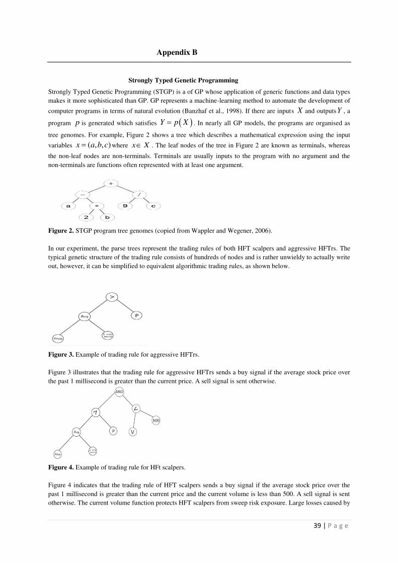
39 | P a g e

Appendix B

Strongly Typed Genetic Programming

Strongly Typed Genetic Programming (STGP) is a of GP whose application of generic functions and data types

makes it more sophisticated than GP. GP represents a machine-learning method to automate the development of

computer programs in terms of natural evolution (Banzhaf et al., 1998). If there are inputs and outputs , a

program is generated which satisfies . In nearly all GP models, the programs are organised as

tree genomes. For example, Figure 2 shows a tree which describes a mathematical expression using the input

variables where . The leaf nodes of the tree in Figure 2 are known as terminals, whereas

the non-leaf nodes are non-terminals. Terminals are usually inputs to the program with no argument and the

non-terminals are functions often represented with at least one argument.

Figure 2. STGP program tree genomes (copied from Wappler and Wegener, 2006).

In our experiment, the parse trees represent the trading rules of both HFT scalpers and aggressive HFTrs. The

typical genetic structure of the trading rule consists of hundreds of nodes and is rather unwieldy to actually write

out, however, it can be simplified to equivalent algorithmic trading rules, as shown below.

Figure 3. Example of trading rule for aggressive HFTrs.

Figure 3 illustrates that the trading rule for aggressive HFTrs sends a buy signal if the average stock price over

the past 1 millisecond is greater than the current price. A sell signal is sent otherwise.

Figure 4. Example of trading rule for HFt scalpers.

Figure 4 indicates that the trading rule of HFT scalpers sends a buy signal if the average stock price over the

past 1 millisecond is greater than the current price and the current volume is less than 500. A sell signal is sent

otherwise. The current volume function protects HFT scalpers from sweep risk exposure. Large losses caused by

X Y

p Y p X

( , , )x a b c x X

40 | P a g e

sweeps (adverse price movements against HFT scalpers’ transient positions) can substantially reduce or even eliminate their profitability, so the management of sweep risk is of paramount importance for HFT scalpers.

HFT scalpers use the market microstructure to capture and avoid sweep risk, which is the risk related to trading

against large informed toxic orders (for instance, large institutional orders) positioned at multiple levels of the

order book.

The fitness function of trading rules of 50,000 HFT scalpers and 50,000 aggressive HFTrs are based on its

ability to satisfy . If is the expected known output and the actual output generated by a

program with , the fitness function of has been calculated as:

(11)

Usually the nodes of the GP tree are not typed as Montana (2002) argues that many GP procedures can be

formulated in a more efficient programming way by implementing a typing mechanism for GP nodes. In this

way each node is connected to a particular return type and the process is known as Strongly Typed Genetic

Programming (STGP). To create a parse tree one needs to take into account important additional programming

criteria such as when the root node of the tree returns a value of the type required by the problem and when each

non-root node returns a value of the type required by the parent node as an argument (Montana, 2002). While

GP can be written in any programming language, the STGP is typically written in a specific programming

language, which is a combination of Ada (Barnes, 1982) and Lisp (Steele, 1984). The concept of generics as a

method of developing strongly typed data is the critical component adopted from Ada. Additionally, Lisp

incorporates the concept of having programs represented by their actual parse trees (Montana, 1995).

In conventional GP, one needs to specify all the programs and variables that can be used as nodes in a parse tree

and deal with the search space of the order of 1030 - 1040. STGP however reduces the searching state-space size

to a greater degree (Montana, 1994). On the other hand, the STGP search space composes the set of all legal

parse trees, which means that all functions have the correct number of parameters of the correct type. On most

occasions, the STGP parse tree is limited to a certain maximum depth (Table 1 illustrates that 20 is the

maximum depth in the three artificial stock markets in this study). We set the maximum depth to 20 in order to

keep the search space finite and manageable, while not allowing the trees to grow to an extremely large size.

The critical concepts in STGP are generic functions (a mechanism for specifying a class of functions), and the

process of assigning generic data types for these functions (Haynes et al., 1995).

STGP has the flexibility to allow all variables, constraints, arguments and returned values to be of any type. The

only strict requirement is that the type of data for each element has to be specified during the early stage of the

programming process. The resulting initialisation process and the various genetic operators associated with it are

enabled to create syntactically correct trees. Those trees on the other hand are beneficial to the entire

programming process because the search space can be significantly reduced (Haynes et al., 1996).

The STGP generates trading rules through the crossover and mutation operators. During the process of

crossover, the return value type of the two selected subtrees for the exchange are examined to find out whether

they are from the same type and that the resulting trees are not breaching depth restrictions. In the case that

either check fails, then two completely new subtrees are selected. If, after performing a finite number of

selections, there are no valid crossover points, then the two parent trees are copied and transferred into the pool

for the next generation (Koza, 1992).

STGP trading rules for the HFT scalpers and aggressive HFTrs can be described through the following

crossover process. Similar to GP, randomly chosen parts of two trading rules are exchanged in order to create

two new trading rules (Figure 3).

( )Y p X expY PY

p ( )p

Y p X ( )f p p

2

exp

1

( )i

X

i

i

f p p x y

41 | P a g e

Figure 3. The process of crossover in STGP for generating new trading rules (copied from Chakraborti et al.,

2011).

Figure 3 illustrates that the trading strategies and are the two parents. The breaking point is based on

random choice and then one-point crossover is applied to create new trading rules (children) and .

The first generation of trading rules is created randomly to ensure that a large variety of possible trading rules is

investigated at full capacity. The best performing trading rules from the initial selection are selected based on

the Breeding Fitness Return to act as parents in the crossover process. The Breeding Fitness Return process

represents a trailing return of a wealth moving average and is an integral part of the latency of HFT scalpers.

This is in fact the return over the last quotes of an exponential moving average of a trader’s wealth, where could potentially have the maximum breeding value of 250. Each pair of parents generates two offspring trading

rules, making the number of parents and the number of offspring equal at all times.

In this innovative programming process, the newly created trading rules replace those that are performing poorly

in the initial selection based on the Replacement Fitness Return. This type of return represents the average

return of a wealth moving average per millisecond quote since the creation of the very first trading rule. In other

words, this is the cumulative return of an exponential moving average of a trader’s wealth, divided by the trader’s breeding value.

iSj

S

kSIS

n n

a note on the relationship between high-frequency trading

Documents