a note on the connection between the primal-dual and the ...xye/papers_and_ppts/papers/the...

International Journal of Operations Research and Information Systems, 1(1), 73-85, January-March 2010 73

Copyright © 2010, IGI Global. Copying or distributing in print or electronic forms without written permission of IGI Globalis prohibited.

Keywords: A* Algorithm, Primal-Dual, Shortest Path

INTRODUCTION

The primal-dual algorithm (Bertsimas & Tsitsik-lis, 1997; Dantzig, Ford, & Fulkerson, 1956; Papadimitriou & Steiglitz, 1998) for linear pro-gramming is very effective for solving network flow problems. Despite the name, the method that we discuss in this article is not to be con-fused with the currently well-known primal-dual interior methods. The latter were originated by Karmarkar’s seminal paper (Karmarkar, 1984) and they enjoy polynomial time-complexity for solving general linear programming problems (Wright, 1997) and have been generalized for

some convex conic optimization problems like second-order cone programming and semi-definite programming (Boyd & Vandenberghe, 2004). The primal-dual algorithm discussed in this article starts from an initial dual feasible solution and iteratively improves the solution until a primal feasible solution, determined by the current dual solution, is found such that the pair satisfies the complementary slackness conditions (Bertsimas & Tsitsiklis, 1997). In this article, we consider the primal-dual algorithm for the shortest path problem in a positively weighted graph equipped with extra information and study the consequence of choosing a proper initial feasible solution to the dual.

a Note on the Connection Between the Primal-Dual

and the a* algorithmXugang Ye, Johns Hopkins University, USA

Shih-Ping Han, Johns Hopkins University, USA

Anhua Lin, Middle Tennessee State University, USA

aBSTRaCTTheprimal-dualalgorithmforlinearprogrammingisveryeffectiveforsolvingnetworkflowproblems.Forthemethod to work, an initial feasible solution to the dual is required. In this article, we show that, for the shortest path problem in a positively weighted graph equipped with a consistent heuristic function, the primal-dual algorithm will become the well-known A* algorithm if a special initial feasible solution to the dual is chosen. We also show how the improvements of the dual objective are related to the A* iterations.

DOI: 10.4018/joris.2010101305

74 International Journal of Operations Research and Information Systems, 1(1), 73-85, January-March 2010


The key point of this article is to utilize the extra information, or heuristic in the language of the field of artificial intelligence, of the graph to construct an initial feasible solution to the dual. We show that the well-known A* algorithm (Hart, Nilsson, & Rapheal, 1968; Hart, Nilsson, & Rapheal 1972; Nilsson, 1980; Pearl, 1984) can be derived. This derivation actually goes directly from the primal-dual algorithm to the A* algorithm. Furthermore, we show how the improvements of the dual objective are related to the A* iterations.

This article is organized as follows. We first set up the problem domain and introduce the A* algorithm and the primal-dual algorithm. We then use the heuristic to construct an ini-tial feasible solution to the dual and propose a best-first search (Pearl, 1984) version of the primal-dual algorithm. We show that this version of the primal-dual algorithm behaves essentially the same as the A* algorithm that uses the same heuristic. Finally, we provide additional discussions.

BaCKGROUND

We consider a directed, positively weighted simple graph denoted as G = (V, A, W, δ, b), where V is the set of nodes, A is the set of arcs, W: A → R is the weight function, δ > 0 is a con-stant such that δ ≤ W(a) < +∞ for all a ∈ A, and finally b is a constant integer such that 0 < b < |V| and |{v | (u, v) ∈ A or (v, u) ∈ A}| ≤ b for all u ∈ V. Suppose we want to find a shortest s-t (directed) path in G, where s ∈ V is a specified starting node and t ∈ V is a specified terminal node. Further suppose a heuristic function ex-ists h: V→ R such that h(v) ≥ 0 for all v ∈ V, h(t) = 0, and W(u, v) + h(v) ≥ h(u) for all (u, v) ∈ A. h is called consistent heuristic. According to Hart et al. (1968), Hart et al. (1972), Nilsson (1980), and Pearl (1984), the A* algorithm that uses such h is complete, that is, it can find a shortest s-t path in G as long as there exists an s-t path in G. The algorithm can be stated as follows. It searches from s to t.

The a* algorithm

Notations:h: heuristicO: Open listE: Closed listd: distance labelf: node selection keypred: predecessor

Steps: Given G, s, t, and h Step 1. Set O = {s}, d(s) = 0, and E = φ. Step 2. If O = φ and t ∈ E, then stop (there is

no s-t path); otherwise, continue. Step 3 . Find u =

Ov∈minarg f(v) = d (v) + h(v).

Set O = O \ {u} and E = E ∪{u}. If t ∈ E , then s top (a s hortest s-t p ath is found); otherwise, continue.

Step 4. For each node v ∈ V such that (u, v) ∈ A and v ∈ E, if v ∈ O, then

set O = O ∪{v}, d(v) = d(u) + W(u, v), and pred(v) = u;

otherwise, if d(v) > d(u) + W(u, v), then

set d(v) = d(u) + W(u, v) and pred(v) = u.

Go to Step 2.

In particular, when h = 0, the A* algorithm stated above reduces to the Dijkstra’s algorithm (Ahuja, Magnanti, & Orlin, 1993; Dijkstra, 1959; Papadimitriou & Steiglitz, 1998). For convenience, for any two nodes u ∈ V and v ∈ V, let dist(u, v) denote the distance from u to v in G. That is, if there is no u-v path in G, we define dist(u, v) = +∞; otherwise, we define dist(u, v) to be the length of a shortest u-v path in G. According to Hart et al. (1968) and Pearl (1984), a central property, called strong optimal-ity, of the A* algorithm stated above is d(u) = dist(s, u) when u ∈ E. If G is a large and sparse finite graph in the sense that b << |V|, then the algorithm can be efficiently implemented by storing G in the form of adjacency lists (Cor-men, Leiserson, Rivest, & Stein, 2001) and maintaining the Open list O as a binary heap,



or pairing heap, or Fibonacci heap (Ahuja et al. 1993; Cormen et al. 2001). For example, using a binary heap to maintain O yields a total number of operations bounded by O(|Efinal|⋅b⋅log2|Omax|) upon successful termination, where Efinal is the final Closed list, Omax is the Open list of the largest size during the iterations, and “O” stands for the “big O” notation. In the worst case, this bound is just O(|A|⋅log2|V|), which is the worst-case time-complexity of the Dijkstra’s algorithm for the single-source shortest path problem using the binary heap implementation. The actual running time of the A* algorithm, however, is determined by dist(s, t), h, and the data structure in implementation. One important result in the A* literature says that the better the heuristic function h, the smaller the size of Efinal. We leave this to the discussions in the later sections.

Given a consistent heuristic h, we can de-fine a new weight function Wh such that Wh(u, v) = W(u, v) + h(v) – h(u) for all (u, v) ∈ A. This change of weights results in a new graph Gh = (V, A, Wh, δ, b). It has been known from Ahuja et al. (1993) that running the Dijkstra’s algorithm to find a shortest s-t path in Gh is equivalent to running the A* algorithm stated above to find a shortest s-t path in G if the two algorithms apply the same tie-breaking rule. The equivalence is due to the fact that the two algorithms construct identical shortest path tree that is rooted at s although the distance labels of the same leaf are distinct. The equivalence tells that the two algorithms can be derived from each other.

Now consider modeling the shortest path problem as linear programming (LP). For convenience, we define G = (V, A , W , δ, b), where A = {(u, v) | (v, u) ∈ A} and W (u, v) = W(v, u) for all (u, v) ∈ A , that is, G is formed by reversing the directions of all the arcs of G. To find a shortest s-t path in G is equivalent to find a shortest t-s path in G . For each (u, v) ∈ A , let x(u, v) denote the decision variable. A primal LP model for finding a shortest t-s path in G is

Min( , )

( , ) ( , )u v A

W u v x u v∈

⋅∑

Subject to

:( , )

( , )v u v A

x u v∈

∑

−:( , )

( , )v v u A

x v u∈

∑

x(u, v) ≥ 0 for all (u, v) ∈ A .

(P)

(2.1)

(2.2)

(2.3)

1 if u = t; −1 if u = s; 0 for all u ∈ V \ {s, t},

=

As long as an s-t path exists in G, it can be easily shown that a binary optimal solution to Model (2.1-2.3) exists. In fact, Model (2.1-2.3) is just to send a unit flow from a supplier t to a customer s in G with least cost. The price of sending a unit flow along any (u, v) ∈ A is W(u, v). One option is to find a shortest t-s path in G and send a unit flow along this path. The general option is to divide the unit flow into pieces. However, to minimize the cost, each piece must be sent along a shortest t-s path in G. This backward version of the primal LP model has a very nice dual, which can be expressed only with respect to G. To show this, we can first write down the dual of Model (2.1-2.3) with respect to G . It is

Max π(t) − π(s) Subject to π(u) − π(v) ≤W (u, v)

for all (u, v) ∈ A ,

(D) (2.5)

(2.4)

where for each v ∈ V, π(v) is the decision vari-able, which is also known as the potential of v. Note that for each (u, v) ∈ A , (v, u) ∈ A and vice versa. And also note that W (u, v) = W(v, u). Hence Constraint (2.5) can be rewritten as

π(u) − π(v) ≤ W(v, u) for all (v, u) ∈ A. (2.6)

By exchanging the arguments u and v, we can further rewrite (2.6) into



π(v)−π(u)≤W(u,v)forall(u,v)∈ A. (2.7)

Constraint (2.7) says that for each (u, v) ∈ A, a triangle inequality relative to s holds as the following Figure 1 shows. Hence, if the primal is the model of searching from t to s in G , then the dual is the model of searching from s to t in G. Conversely, if the primal is the model of searching from s to t in G, then the dual is the model of searching from t to s in G .

An obvious advantage of (D) is that a fea-sible solution is easy to find. At least, π = 0 is one. The key idea of the primal-dual algorithm for the shortest path problem, illustrated in Pa-padimitriou and Steiglitz (1998), is to start from a feasible solution π to (D), search for a feasible solution x to (P) such that for each (u, v) ∈ A, x(u, v) = 0 whenever W(u, v) − π(v) + π(u) > 0. If such x is found, then a shortest s-t path in G can be found. In fact, such x corresponds to an s-t path on which for each arc (u, v), the equality W(u, v) − π(v) + π(u) = 0 holds. If such x cannot be found, then some procedure is needed to up-date π such that Constraint (2.7) is still satisfied and Objective (2.4) is improved. An important feature of the primal-dual algorithm is that any equality in Constraint (2.7) still holds after π is updated. Another important feature is that after π is updated, one strict inequality in Constraint (2.7) may become equality. The primal-dual algorithm keeps attempting to construct an s-t path in G by using the arcs that correspond to the equalities in Constraint (2.7). According to Papadimitriou and Steiglitz (1998), given the initial feasible solution π = 0 to (D), the primal-dual algorithm behaves essentially as same as

the Dijkstra’s algorithm that searches from s to t in G. Hence the Dijkstra’s algorithm can be derived from the primal-dual algorithm.

The two known results show that the A* algorithm with consistent heuristic h can be derived from the primal-dual algorithm. But the derivation needs the Dijkstra’s algorithm as the bridge. It also involves the change of the weight function. In this article, we show that if we use h to construct an initial feasible solution to (D), then applying the primal-dual algorithm directly leads to the A* algorithm that searches from s to t in G.

DERIVaTION

The key point of our derivation is to choose π(0) = − h as the initial feasible solution to (D). To justify the dual feasibility of π(0), we notice, by the consistency of h, that W(u, v) + h(v) ≥ h(u) for all (u, v) ∈ A. Hence, W(u, v) − π(0)(v) ≥ −π(0)(u) for all (u, v) ∈ A. The inequality can be rewritten as π(0)(v) − π(0)(u) ≤ W(u, v), which is exactly what the dual feasibility requires.

A nice property of (D) is that it does not require its solution to be nonnegative. Although π(0) = − h ≤ 0, what really matters is π(0)(t) − π(0)(s) = − h(t) + h(s) = h(s) ≥ 0. This means π(0) = − h is a better initial feasible solution to (D) than π(0) = 0. But we still need to justify the validity of π(0) = − h. That is, we still need to show that the primal-dual algorithm that starts from the solution π(0) = −h to (D) can find a shortest s-t path in G as long as there exists an s-t path in G. It suffices to show the equivalence between the primal-dual algorithm that starts from − h

Figure 1. Triangle inequality relative to s for arc (u, v) in G

s t

u

vπ(v)

π(u)W(u, v)



and the A* algorithm that uses h. We now give the description of the best-first search version of the primal-dual algorithm that starts from − h as follows:

algorithm 1

Notations:h: heuristicO: Open listE: Closed listπ : potentialf1: node selection keypred: predecessorθ: potential incrementΦ: cumulative potential increase

Steps: Given G, s, t, and h Step 1. Set Φ = 0. Set O = {s}, π(s) = −h(s),

pred(s) = s, and E = φ. Set W(s, s) = 0. Step 2. If O = φ and t ∈ E, then stop (there is

no s-t path); otherwise, continue. Step 3. Find u = arg min

v O∈f1(v) = W(pred(v), v)

− π(v) + π(pred(v)). Set θ = W(pred(u), u) − π(u) + π(pred(u)). Set Φ = Φ + θ. Set O = O \ {u} and E = E ∪{u}. Set π(u) = −h(u) + Φ. If t ∈ E, then stop (a shortest s-t path is found); otherwise, continue.

Step 4. For each v ∈ O, set π(v) = −h(v) + Φ. Step 5 . For each v ∈ V such that (u, v) ∈ A

and v ∈ E, if v ∈ O, then

set O = O ∪{v}, pred(v) = u, and π(v) = −h(v) + Φ;

otherwise, if W(pred(v), v) + π(pred(v)) > W(u, v) + π(u), then

set pred(v) = u. Go to Step 2.

For theoretical convenience, right after Step 5, for all v ∈ V \ (E∪O), we define π(v) = −h(v) + Φ. We can show that Algorithm 1, just like the classical version (Papadimitriou & Steiglitz, 1998) of the primal-dual algorithm, maintains the dual feasibility throughout.

Proposition 1: The dual feasibility stated as Constraint (2.7) is maintained when running Algorithm 1.

Proof. The proof is inductive. The base case is upon the completion of the first iteration. At this moment, π = π(0), it’s trivially true. Sup-pose right before the k-th iteration (k > 1), the potential of any v ∈ V is π(v) and π satisfies the dual feasibility. We need to show that right after the k-th iteration, the dual feasibility is still maintained. Right before the k-th itera-tion, let [E, O] denote the E-O cut, which is the set of arcs from E to O. We only need to show that the node selection rule in Step 3 of Algorithm 1 is equivalent to finding an arc (u, v) ∈ [E, O] such that W(u, v) − π(v) + π(u) is the minimum. In fact,

( , ) [ , ]min

u v E O∈[W(u, v) − π(v) + π(u)]

= minv O∈

( , ) [ , ]

minu E

u v E O∈

∈

[W(u, v) − π(v) + π(u)]

= minv O∈

( , ) [ , ]

min [ ( , ) ( )] ( )u E

u v E O

W u v u vπ π∈

∈

+ −

= minv O∈

[W(pred(v), v) + π(pred(v)) − π(v)].

Hence, the node selection rule in Step 3 of Algorithm 1 is equivalent to the arc selection rule in the classical version of the primal-dual algorithm. Note that the later one guarantees the satisfaction of the dual feasibility right after the k-th iteration; therefore, the proposition is true. Q.E.D.

From Algorithm 1 we can see that the po-tentials of the nodes that have entered the Closed list E become permanent. Furthermore, we can show that the potential difference between any u ∈ E and s is actually the length of the shortest s-u path in G.

Proposition 2: After each iteration of Algorithm 1, π(u) − π(s) = dist(s, u) for any node u ∈ E.

Proof: When node u enters E, an s-u pointer path, say P: v1 (= s) ~ v2 ~ … ~ vk (= u), is



determined. Denote L(P) as the length of P. Note that π(v2) = W(v1, v2) + π(v1), …, π(vk) = W(vk-1, vk) + π(vk-1). By telescoping, we have π(vk) = L(P) + π(v1), that is, π(u) − π(s) = L(P). Since there is an s-u path in G, there must be a shortest s-u path in G. This is because any s-u path in G with length no longer than L(P) has only finite number of arcs, hence the number of s-u paths in G with length no longer than L(P) is finite. Let

P : v1

(= s) ~ v2~ … ~ v

k(= u) be

a shortest s-u path in G and denote L(

P ) as the length of

P . By Proposition 1, Algorithm 1 maintains the dual feasibility stated as Constraint (2.7). Hence π( v

2) ≤ W( v

1, v

2) + π( v

1), …,

π( vk

) ≤ W(

vk-1 , v

k) + π( v

k-1). By telescop-

ing, we have π( vk

) ≤ L(

P ) + π( v1

), that is, π(u) − π(s) ≤ L(

P ). The two arguments jointly imply that P is in fact a shortest s-u path and π(u) − π(s) = dist(s, u). Q.E.D.

We now show the equivalence between Algorithm 1 and the A* algorithm we listed at the beginning.

Proposition 3: Under the same tie-breaking rule, Algorithm 1 is equivalent to the A* algo-rithm that uses h, searching from s to t.

Proof: The proof is inductive. We need to show that right after each same iteration, the two algorithms have the same Open list and Closed list, and for each node in the Open list, the two algorithms assign the same predecessor in the Closed list. The base case is upon the comple-tion of the first iteration of the two algorithms, respectively. Note that in the base case, s is the only node “closed” by the two algorithms. Hence, the base case is trivially true. Suppose (inductive hypothesis) right before the k-th it-eration (k > 1) of the two algorithms, the claim above is true. We now show that the claim still holds right after the k-th iteration.

Firstly, we need to show that the node selec-tion rule in Step 3 of Algorithm 1 is equivalent to the node selection rule in the A* algorithm.

Consider the moment Algorithm 1 is about to enter its Step 3. At this moment, (arbitrarily) consider a node v ∈ O. Note that v must have a predecessor, say u ∈ E. The selection key of v is W(u, v) − π(v) + π(u). Note that

W(u, v) − π(v) + π(u)= W(u, v) − (−h(v) + Φ) + π(u)= W(u, v) + π(u) − π(s) + h(v) − Φ + π(s).

By Proposition 2, we have

π(u) − π(s) = dist(s, u).

Hence

W(u, v) − π(v) + π(u)= W(u, v) + dist(s, u) + h(v) − Φ + π(s).

We can see that W(u, v) + dist(s, u) = W(u, v) + d(u) = d(v) and d(v) + h(v) = f(v). Also note that both Φ and π(s) remain the same when different nodes in O are considered. Hence, by inductive hypothesis, under the same tie-breaking rule, Algorithm 1 selects the same node from O as the A* algorithm.

Secondly, we need to show that, under the same tie-breaking rule, after a node, say u, is removed from O and put into E in Step 3 of Algorithm 1, the predecessor update on any node v ∈ O is as same as that in the A* algorithm. In fact, if there is no arc (u, v) ∈ A, there won’t be any predecessor update on v. If there is an arc (u, v) ∈ A, then in Algorithm 1, the update is based on comparing W(pred(v), v) + π(pred(v)) with W(u, v) + π(u). By Proposition 2 again,

W(pred(v), v) + π(pred(v))= W(pred(v), v) + π(pred(v)) − π(s) + π(s)= W(pred(v), v) + dist(s, pred(v)) + π(s)

and

W(u, v) + π(u)= W(u, v) + π(u) − π(s) + π(s)= W(u, v) + dist(s, u) + π(s).



Note that π(s) is common; hence, the comparison is actually between W(pred(v), v) + dist(s, pred(v)) = d(v) and W(u, v) + dist(s, u) = W(u, v) + d(u). Under the same tie-breaking rule, this is just the predecessor update rule in the A* algorithm.

Finally, note that if there is a node v ∈ V \ (E∪O) such that (u, v) ∈ A, then Algorithm 1 will put it into O and assign it a predecessor u. Hence W(pred(v), v) + π(pred(v)) = W(u, v) + π(u) = W(u, v) + dist(s, u) + π(s), which implies that v receives a distance label d(v) = W(u, v) + dist(s, u). This is just what the A* algorithm does.

Combine the three arguments above, we have shown that the two algorithms maintain the same Open list and Closed list, and for each node in the Open list, they assign the same predecessor in the Closed list. Q.E.D.

The original version of the primal-dual in Papadimitriou and Steiglitz (1998) selects an arc in E-O cut and adds the head of this arc into E. Other than manipulating the arc selection, Algorithm 1 manipulates the node selection in each iteration. Although the A* algorithm is algorithmically different from Algorithm 1, they behave the same. Those equivalences imply that the time-complexity of the A* algorithm should also be valid for the primal-dual algo-rithm. And indeed, the A* algorithm is a good implementation of the primal-dual algorithm that starts from π(0) = −h.

DUalITY

There is a nice property of the A* algorithm that uses consistent heuristic. For the A* al-gorithm we listed at the beginning, suppose a node u1 is closed no later than another node u2, then according to Hart et al. (1968) and Pearl (1984), f(u1) ≤ f(u2). This property is called monotonicity. By monotonicity, before t is closed, for any closed node u, f(u) ≤ dist(s, t). By combining the monotonicity property of the A* algorithm and Algorithm 1, we have the following interesting result.

Proposition 4: After each iteration of Algorithm 1, π(t) − π(s) = max

u EÎ f(u) ≤ dist(s, t).

Proof. The inequality directly follows from the monotonicity property. We now show the equality. Consider any iteration of Algorithm 1. Suppose node u is selected in Step 3 during this iteration. Upon the completion of this itera-tion, by the proof of Proposition 3, we see that Φ = f(u) + π(s); also note that π(t) = − h(t) + Φ = Φ, hence π(t) − π(s) = f(u). By monotonicity property, upon the completion of this iteration, f(u) = max

'u EÎf(u ′). Q.E.D.

If we define d(t) = +∞ when t ∈ E∪O, we then have that π(t) − π(s) ≤ d(t) always holds. This is because d(t) ≥ dist(s, t) always hold. The inequality π(t) − π(s) ≤ d(t) can be viewed as the weak duality. The duality gap is d(t) − (π(t) − π(s)) = d(t) − max

u EÎf(u). As the primal

objective, d(t) is monotonically nonincreasing; as the dual objective, π(t) − π(s) = max

u EÎf(u) is

monotonically increasing. By completeness, if there exists an s-t path in G, then t will eventu-ally be closed. Upon the moment t is closed, we have max

u EÎf(u) = f(t) = d(t). Hence, both

π(t) − π(s) and d(t) reach optimal. This means the duality gap is eliminated. The final equality is just the so-called strong duality.

Just like the A* algorithm, Algorithm 1 may terminate at its Step 2. Simple analysis (Pearl, 1984) of the A* algorithm tells that termination at Step 2 implies there is no s-t path in G. An explanation within the primal-dual framework is that when Algorithm 1 terminates at its Step 2, the potentials of all nodes outside E can be arbitrarily raised the same value without violating Constraint (2.7). But the objective (2.4) will be unbounded. This just implies the infeasibility of (P). Just like the A* algorithm, Algorithm 1 may not terminate at all. This hap-pens when there is no s-t path in G, but there are infinitely many nodes that are connected with s via paths. Under this circumstance, the objective (2.4) is also unbounded. We conclude this section with a numerical example that



demonstrates how the A* iterations improve the dual objective (2.4).

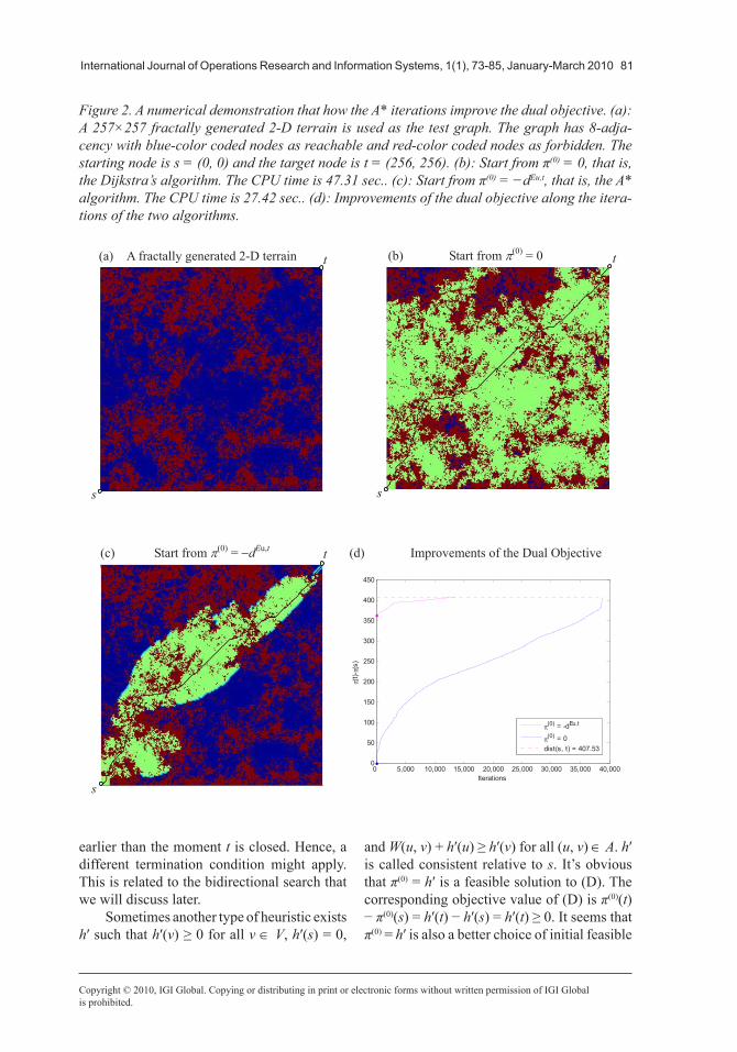
As shown in Figure 2, a 257×257 2-D ter-rain is fractally generated using the diamond square algorithm (Miller, 1986) as the test graph. The graph is a grid with 8-adjacency with blue-color coded nodes as reachable and red-color coded nodes as forbidden. The starting node is s = (0, 0) and the target node is t = (256, 256). The subfigures (b) and (c) display the search results associated with π(0) = 0 (the Dijkstra’s algorithm) and π(0) = −dEu,t (the A* algorithm), respectively. Both algorithms were coded with Matlab 7.1 and tested in a PC with Intel dual core CPU T2050 at 1.6 GHz and 1.0 G RAM. The notation dEu,t stands for the Euclidean distance with respect to the target node t, that is, for any reachable node v, dEu,t(v) denotes the Euclidean distance between v and t. Obviously, dEu,t is a consistent heuristic in the A* search. In both (b) and (c), the green-color coded nodes represent those that have been closed when t is closed. The black curves are the shortest s-t paths that are found by the two algorithms. The subfigure (d) displays how the dual objective is iteratively improved by the two algorithms. It can be seen that, in this numerical instance, the A* algorithm needs much less iterations than the Dijkstra’s algorithm. Although the computational cost of evaluating the heuristic in the A* search is involved, substantially less iterations lead to the much better overall efficiency.

INITIal FEaSIBlE SOlUTIONS

Our analysis so far tells that the selection of π(0) = – h is sound. Actually, –h defines a class of initial feasible solutions to (D). Suppose we have two consistent heuristics h1 and h2. Denote PDi as the primal-dual algorithm starting from –hi, i = 1, 2. By completeness, both PD1 and PD2 will successfully terminate as long as there exists an s-t path in G. If h1(v) > h2(v) for all v ∈ V \ {t} and there exists an s-t path in G, then A dominance theorem (Hart et al. 1968; Nilsson, 1980; Pearl, 1984) on the A* algorithm says that E1 ⊆ E2, where Ei denotes the final Closed list of PDi, i = 1, 2.

There are two interesting extreme cases. One is that π(0) = 0. We have seen, in this case, that Algorithm 1 reduces to the Dijkstra’s al-gorithm. This just indicates the derivation of the Dijkstra’s algorithm from the primal-dual algorithm. The other is that π(0)(v) = − dist(v, t) for all v ∈ V. In this case, Algorithm 1 only closes the nodes that lie on a shortest s-t path in G, hence the initial feasible solution to (D) is perfect.

Sometimes, there exits some metric func-tion H: V×V → R such that H(u, v) ≥ 0 for all u, v ∈ V, H(v, v) = 0 for all v ∈ V, and W(u, v) + H(v, w) ≥ H(u, w) for all (u, v) ∈ A. We im-mediately have a consistent heuristic, say hH, defined as hH(v) = H(v, t) for all v ∈ V. Under some condition, we can also find another consis-tent heuristic. Suppose we already have a partial solution that is represented by a shortest path tree T of G rooted at t. Suppose this shortest path tree is found by the Dijkstra’s algorithm that searches from t to s in G . Let ET and OT denote the Closed list and Open list associated with T. We define

hH,T(v) =

minTOτ∈

[H(v, τ) + dist(τ, t)]

for all v ∈ V \ ET;

dist(v, t) for all v ∈ ET.

(5.1)

It can be easily shown that hH,T is a con-sistent heuristic, and for any v ∈ V, as the two estimates of dist(v, t), hH,T(v) is at least as good as hH(v), that is, hH(v) ≤ hH,T(v) ≤ dist(v, t). The primal-dual algorithm can start from π(0) = −hH if H is available. The primal-dual algorithm can also start from π(0) = −hH,T if both H and T are available. In the case that both H and T are available, to start from −hH,T may result in less closed nodes upon closing t than to start from −hH, but it doesn’t mean that the former has better efficiency since to evaluate hH,T by (5.1) is more costly than to evaluate hH. However, an issue that should be addressed is that the primal-dual algorithm that starts from −hH,T may be able to successfully find a solution



earlier than the moment t is closed. Hence, a different termination condition might apply. This is related to the bidirectional search that we will discuss later.

Sometimes another type of heuristic exists h′ such that h′(v) ≥ 0 for all v ∈ V, h′(s) = 0,

and W(u, v) + h′(u) ≥ h′(v) for all (u, v) ∈ A. h′ is called consistent relative to s. It’s obvious that π(0) = h′ is a feasible solution to (D). The corresponding objective value of (D) is π(0)(t) − π(0)(s) = h′(t) − h′(s) = h′(t) ≥ 0. It seems that π(0) = h′ is also a better choice of initial feasible

Figure 2. A numerical demonstration that how the A* iterations improve the dual objective. (a): A 257×257 fractally generated 2-D terrain is used as the test graph. The graph has 8-adja-cency with blue-color coded nodes as reachable and red-color coded nodes as forbidden. The startingnodeiss=(0,0)andthetargetnodeist=(256,256).(b):Startfromπ(0) = 0, that is, theDijkstra’salgorithm.TheCPUtimeis47.31sec..(c):Startfromπ(0)=−dEu,t, that is, the A* algorithm. The CPU time is 27.42 sec.. (d): Improvements of the dual objective along the itera-tions of the two algorithms.

s

t(a) A fractally generated 2-D terrain

(c) Start from π(0) = −dEu,t

s

t

(b) Start from π(0) = 0

s

t

0 5,000 10,000 15,000 20,000 25,000 30,000 35,000 40,0000

50

100

150

200

250

300

350

400

450

Iterations

π(t)-π(

s)

π(0) = -dEu,t

π(0) = 0dist(s, t) = 407.53

(d) Improvements of the Dual Objective

Figure 2: A numerical demonstration that how the A* iterations improve the dual objective. (a): A 257×257 fractally generated 2-D terrain is used as the test graph. The graph has 8-adjacency with blue-color coded nodes as reachable and red-color coded nodes as forbidden. The starting node is s = (0, 0) and the target node is t = (256, 256). (b): Start from π(0) = 0, that is, the Dijkstra’s algorithm. The CPU time is 47.31 sec.. (c): Start from π(0) = −dEu,t, that is, the A* algorithm. The CPU time is 27.42 sec.. (d): Improvements of the dual objective along the iterations of the two algorithms.



solution to (D) than π(0) = 0, however, the follow-ing simple example shows that the primal-dual algorithm that starts from h′ may not terminate at all even if an s-t path exists in G.

Figure 3 shows a simple infinite graph. We want to find a shortest s-t path. When applying the primal-dual algorithm with π(0) = {h′(s) = 0, h′(u) = 0, h′(t) = 0, and h′(vi) = i for i = 1, 2, …} as the initial feasible solution to (D), the algorithm (Algorithm 1 with initial node potential function set as this π(0)) will close s at first, then v1, then v2, …. Note that u will never be closed, let alone t. Hence, the algorithm won’t be able to successfully terminate. Even if we restrict this graph to be finite and the algorithm is able to terminate, the efficiency is bad because it traverses the wrong way before heading toward the right way.

BIDIRECTIONal SEaRCH

Although h′ is not a proper choice of the initial feasible solution to (D) for Algorithm 1 to start from, it can be used for bidirectional search. Consider the primal LP model with respect to

G, in which for each (u, v) ∈ A, we still use x(u, v) to denote the decision variable:

Min ( , )

( , ) ( , )u v A

W u v x u v∈

⋅∑

Subject to

:( , )( , )

v u v Ax u v

∈∑ −

:( , )( , )

v v u Ax v u

∈∑

=

x(u, v) ≥ 0 for all (u, v) ∈ A.

(P′)

(6.3)

(6.2) 1 if u = s; −1 if u = t; 0 for all u ∈ V \ {s, t}

(6.1)

This forward version of primal LP model stands for sending a unit flow from a supplier s to a customer t in G with least cost. It has the following dual:

Max π(s) − π(t) Subject to π(u) − π(v) ≤ W(u, v)

for all (u, v) ∈ A.

(D′) (6.5)

(6.4)

Figure3.Aexamplethattheprimal-dualalgorithmstartingfromsomeπ(0)=h′doesnottermi-nate,wherethelengthofanyarcis1andtheheuristicfunctionh′is{h′(s)=0,h′(u)=0,h′(t)=0,andh′(vi) = i for i = 1, 2, …}



Similar analysis can show that the primal-dual algorithm that uses – h′ as the initial feasible solution to (D′) is essentially the A* algorithm that searches from t to s in G using the heuristic h′. This version of the primal-dual algorithm is exactly the backward version of Algorithm 1. If both algorithms are used, searching toward each other, then a bidirectional A* search can be established. For the backward version of Algorithm 1, let O′, π ′ and pred ′ denote the corresponding Open list, potential function, and predecessor function, respectively. When the two search fronts (Open lists) meet, an s-t path is found, and its length, denoted as L, can be expressed as

L = [W(pred(v), v) + π(pred(v)) − π(s)] +[W(v, pred ′(v)) + π ′(pred ′(v)) − π ′(t)],

where v ∈ O∪O′ is the meeting node. When the search continues, a sequence of lengths, say L1, L2, …, is generated.

Let

L = min{L1, L2, …}, which is the length of the shortest s-t path in G found so far. Since

π(t) − π(s) ≤ dist(s, t) ≤

L and

π ′(s) − π ′(t) ≤ dist(s, t) ≤

L ,

we have a termination condition for the bidirec-tional A* search, expressed via π and π ′, as

max{π(t) − π(s), π ′(s) − π ′(t)} =

L . (6.6)

This condition is essentially as same as the one that appears in Pohl (1971). It can eventu-ally be satisfied.

Again, the bidirectional A* search reduces to the bidirectional Dijkstra’s search when h = h′ = 0. An alternative termination condition, according to Korf and Zhang (2005) and Propo-sition 2, that is expressed via π and π ′, is

minv OÎ

[W(pred(v), v) +π(pred(v)) −π(s)] +

min' 'v OÎ

[W(v′, pred ′(v′)) +π ′(pred ′(v′)) −π ′(t)]

= min' 'v OÎ

L [W(v′, pred ′(v′)) +π ′(pred ′(v′)) −π

′(t)] =

L , (6.7)

which can also eventually be satisfied.

CONClUSION

We have shown that for the shortest path problem in a positively weighted graph equipped with a consistent heuristic function, choosing the initial feasible solution to the dual in the primal-dual algorithm is equivalent to choosing the consis-tent heuristic in the A* algorithm. Although the equivalence between the primal-dual algorithm and the A* algorithm is a known result, there are still questions to answer. One is that how the A* iterations relate to the improvements of the dual objective. Our new derivation of the equivalence is not only a direct and simpler way but also answers this question as stated in Proposition 4. Compared to the Dijkstra’s algorithm in improving the dual objective, the A* search enjoys an initial “leap” of h(s) and the continual role played by the heuristic h during the iterations. Moreover, the completeness of the A* search guarantees that the duality gap can be eventually eliminated if there exists a solution.

Through both the theoretical and numeri-cal investigations, we not only gain a further understanding of the A* algorithm from the primal-dual perspective but also like to pose new questions. For example, it’s still not quite clear on how the primal-dual and the bidirectional search relate to each other. A central issue of the later is to find a good termination condition. Another issue is how to alternatively switch from one direction to the other. Although those two issues have been extensively studied, the idea of looking at the questions from the primal-dual perspective seems to be novel. We suggest a further investigation as a possible extension of the work in this article.



aCKNOwlEDGMENT

The authors would like to thank the editor-in-chief of the journal, Professor John Wang, and the anonymous reviewers for their valuable comments and suggestions that improved the article significantly.

REFERENCES

Ahuja, R. K., Magnanti, T. L., & Orlin, J. B. (1993). Network flows: Theory, algorithms, and applications. Englewood Cliffs, NJ: Prentice Hall.

Bertsimas, D., & Tsitsiklis, J. N. (1997). Introduc-tion to linear optimization. Belmont, MA: Athena Scientific.

Boyd, S., & Vandenberghe, L. (2004). Convex opti-mization. UK: Cambridge University Press.

Cormen, T. H., Leiserson, C. E., Rivest, R. L., & Stein, C. (2001). Introduction to algorithms (2nd ed.). Cambridge, MA: MIT Press.

Dantzig, G. B., Ford, L. R., & Fulkerson, D. R. (1956). A primal-dual algorithm for linear programs. In H. W. Kuhn & A. W. Tucker (Eds.), Linear inequalities and related systems (pp. 171-181). NJ: Princeton University Press.

Dijkstra, E. W. (1959). A note on two problems in connection with graphs. Numerical Mathematics, 1, 269–271. doi:10.1007/BF01386390

Hart, P. E., Nilsson, N. J., & Raphael, B. (1972). Correction to “A formal basis for the heuristic determination of minimum cost paths”. SIGART Newsletter, 37, 28–29.

Hart, P. E., Nilsson, N. J., & Rapheal, B. (1968). A for-mal basis for the heuristic determination of minimum cost paths. IEEE Transactions of System Sciences and Cybernetics, SSC-4, 2(July), 100-107.

Karmarkar, N. (1984). A new polynomial-time algo-rithm for linear programming. COMBINATORICA, 4, 373–395. doi:10.1007/BF02579150

Korf, R. E., & Zhang, W. (2005). Frontier search. Journal of the Association for Computing Machinery, 52(5), 715–748.

Miller, G. (1986). The definition and rendering of terrain maps. Computer Graphics, 20(4), 39–48. doi:10.1145/15886.15890

Nilsson, N. J. (1980). Principles of artificial intel-ligence. San Mateo, CA: Morgan Kaufmann.

Papadimitriou, C. H., & Steiglitz, K. (1998). Com-binatorial optimization: Algorithms and complexity. Mineola, New York: Dover Publications.

Pearl, J. (1984). Heuristics: Intelligent search strate-gies for computer problem solving. Reading, MA: Addison-Wesley.

Pohl, I. (1971). Bidirectional search. In B. Meltzer & D. Michie (Eds.), Machine intelligence 6 (pp. 127-140). New York: Elsevier.

Wright, S. J. (1997). Primal-dual interior-point methods. Philadelphia, PA: Society for Industrial and Applied Mathematics.

Xugang Ye (*) is a research associate in the Department of Applied Mathematics and Statistics, Johns Hopkins University. He obtained his PhD degree from the Department of Applied Mathemat-ics and Statistics, Johns Hopkins University. Dr. Ye has broad research interests in probability, statistics, and optimization and is serving on collaborative research projects from the Department of Electrical Engineering, Duke University, and the Biostatistics Branch, National Institute of Child Health and Human Development. He also presented his research in INFROMS, SIAM, and so forth, and was selected as the Counselman Fellow in Johns Hopkins University.

Shih-Ping Han is a professor in the Department of Applied Mathematics and Statistics, Johns Hopkins University. He obtained his PhD degree from the Department of Computer Sciences, University of Wisconsin at Madison. He had also been a distinguished professor of mathematics



in the University of Illinois at Urbana-Champaign, an assistant professor of computer sciences in Cornell University, and a visiting scholar in Cambridge University. Professor Han is a renowned mathematician in the area of continuous optimization and had published many important results in the journals like mathematical programming and mathematics of operations research.

Anhua Lin is an assistant professor in the Department of Mathematical Sciences, Middle Tennes-see State University. He obtained his PhD degree from the Department of Applied Mathematics and Statistics, Johns Hopkins University. Professor Lin’s research interests include continuous optimization and integer programming. His recent focus is on graph theory and combinatorics. Lin has published several papers in the journals like SIAM Journal on Optimization and Discrete Applied Mathematics. He also presented his research in INFROMS, SIAM, and so forth.

a note on the connection between the primal-dual and the ...xye/papers_and_ppts/papers/the...

Documents