HAL Id: hal-03189322https://hal.archives-ouvertes.fr/hal-03189322

Submitted on 28 Apr 2021

HAL is a multi-disciplinary open accessarchive for the deposit and dissemination of sci-entific research documents, whether they are pub-lished or not. The documents may come fromteaching and research institutions in France orabroad, or from public or private research centers.

L’archive ouverte pluridisciplinaire HAL, estdestinée au dépôt et à la diffusion de documentsscientifiques de niveau recherche, publiés ou non,émanant des établissements d’enseignement et derecherche français ou étrangers, des laboratoirespublics ou privés.

A nongray-wall emissivity model for the Wide-BandCorrelated K-distribution method

Y. Liu, J. Zhu, G. Liu, J.L. Consalvi, Franklin Liu

To cite this version:Y. Liu, J. Zhu, G. Liu, J.L. Consalvi, Franklin Liu. A nongray-wall emissivity model for the Wide-Band Correlated K-distribution method. International Journal of Heat and Mass Transfer, Elsevier,2020, 159 (120095), �10.1016/j.ijheatmasstransfer.2020.120095�. �hal-03189322�

A Nongray-Wall Emissivity Model for the Wide-Band Correlated K-

Distribution Method

Yuying LIUa, Jinyu ZHUa, Guanghai LIU a,*, Jean-louis CONSALVIb, Fengshan LIUc

a. School of Energy and Power Engineering, Beihang University (BUAA), Beijing, 100191, China

b. Aix-Marseille Université, CNRS, IUSTI UMR 7343, 5 rue E. Fermi, 13013 Marseille, France

c. Measurement Science and Standards, National Research Council of Canada, 1200 Montreal Road, Ottawa, Ontario K1A 0R6, Canada

* Corresponding author: ghliu@buaa.edu.cn(G.LIU)

Abstract

The walls of combustion systems are usually assumed to be black or gray in radiative calculations, which may introduce

large errors. The Planck-function-weighted emissivity is usually used as the gray-wall emissivity when using the Wide-Band

Correlated K-distribution (WBCK) method. This approach can demonstrate good accuracy when the emissivity-based

optimized band interval proposed by Solovjov (2013, JQSRT)(WBCK-1) is used. To improve efficiency without losing

accuracy, a nongray-wall emissivity model is proposed. The accuracy of this model is first demonstrated for the emissivity-

based band interval (WBCK-2). An absorption-coefficient-based optimized band interval is then proposed and the accuracy

of this band interval coupled with the nongray-wall emissivity model (WBCK-3) is evaluated. The performance of these

models is evaluated in three 1D isothermal and homogeneous cases bounded by fly-ash deposit, GH536, and soot deposit and

a 3D fuel-air flame bounded by fly-ash deposit. The results show that WBCK-2 is more accurate than WBCK-1 when the

number of bands is greater than 1. WBCK-3 can become more accurate than WBCK-1 and WBCK-2 when the number of

bands is larger than 2, especially for low wall temperatures. Furthermore, it is sufficient to divide the spectrum into 3 bands

for accurate predictions of radiative calculations.

Keywords: Radiative heat transfer; Wide-Band Correlated K-distribution; Emissivity; Nongray wall.

Nomenclature

a non-gray stretching factor in WBCK

f wide-band k-distribution function

g cumulative wide-band k-distribution function

G incident radiation (W/m2)

I radiative intensity (W/sr)

J number of angular ordinates

k reordered spectral absorption coefficient (cm-1)

L length (m)

M number of bands

N number of quadrature points

P total pressure (pa)

Q number of iterations

R radius (m)

T temperature (K)

u direction weight

w quadrature weight

𝒙 mole fraction vector

Greek symbols

Subscripts

b blackbody

m mth band

max maximum

l lower

n nth quadrature point

P Planck

j jth ordinates

u upper

w wall

0 reference state

Abbreviations

FSCK Full-Spectrum Correlated K-distribution

LBL Line-By-Line

MSMGFSK Multi-Scale Multi-Group FSK

NBCK Narrow-Band Correlated K-distribution

RTE radiative heat equation

SLW Spectral-Line-based Weighted-sum-of-gray-gases

SNBCK Statistical Narrow-Band Correlated-K

𝛈 wavenumber (𝐜𝐦−𝟏)

𝜿 spectral absorption coefficient (𝐜𝐦−𝟏)

𝝓 vector of thermodynamic state variables

𝜹 Dirac-delta function

𝛆 emissivity

SNB Statistical Narrow-Band

WBCK Wide Band Correlated-K

WSGG Weighted-Sum-of-Gray-Gases

1. Introduction

Radiative heat transfer plays an important role in high-temperature industrial combustion systems, such as coal-fired boilers

and gas turbine combustors [1]. Most studies assume that the walls of combustors are black or gray in radiative transfer

calculations for simplicity in spite of the fact that the wall materials have different spectral emissivity. This simplification

may introduce large errors in the prediction of radiative source term and heat flux [2], which may strongly affect the predicted

performance of the combustion devices in terms of thermal protection [3] and pollutant emissions [4]. Therefore,

comprehensive and accurate radiative models are necessary for accurately predicting radiative heat transfer in practical

problems involving nongray walls and for optimal design of combustion devices.

Radiative heat transfer models with different spectral resolutions, such as the Line-By-Line method (LBL), narrow-band

models [5]-[], wide-band models [9], [] and full-spectrum models [8], 11]-13], provide different accuracy and computational

efficiency [14]. The benchmark LBL method is rarely applied to practical applications due to the huge requirement in

computing resources [15]. Narrow-band models, such as the Statistical Narrow-Band method (SNB) [5], ], the Statistical

Narrow-Band Correlated-K method (SNBCK) [7] and the Narrow-Band Correlated K-distribution method (NBCK) [8],

demonstrate the best accuracy in comparison to LBL because of small changes in spectral emissivity within a narrow spectral

range for both gases and a solid wall. Although the number of radiative transfer equations (RTEs) of narrow-band models is

much less than that of LBL, the computing resources required for solving narrow-band RTEs are still unacceptable in practical

applications. Therefore, various computationally more efficient wide-band models and full-spectrum models have been

developed. Full-spectrum models, such as the Full-Spectrum Correlated K-distribution method (FSCK) [8], the Spectral-Line-

based Weighted-Sum-of-Gray-Gases method (SLW) [11] and the Weighted-Sum-of-Gray-Gases method (WSGG) [13],

provide the highest computational efficiency at the cost of some accuracy for practical problems involving nongray walls [16],

17]. Wide-band models have a great potential for achieving the best compromise between efficiency and accuracy for practical

problems with nongray walls. For example, Solovjov et al. [16] proposed a method to optimize band interval according to the

spectral emissivity for the expansion of SLW named the cumulative wavenumber model, in which only a few RTEs need to

be solved. Fonseca et al. [17] separated gray gases into several groups according to a presumed emissivity, followed by solving

RTE with the WSGG method. The banded method was employed by Bordbar et al. [18], 19] to solve such problems as well.

It was shown that those methods provide a good compromise between accuracy and efficiency for nongray wall problems.

The Planck-function-weighted emissivity at the wall temperature is usually used as the gray-wall emissivity to ensure the

conservation of radiative energy at the wall [14]. This gray-wall emissivity model can achieve good accuracy when combined

with the emissivity-based optimized band interval mentioned above [16] for nongray wall problems too. To further improve

computational efficiency without significantly losing accuracy, some methods have been proposed recently. For instance,

Fonseca et al. [20] used a radiating medium mean temperature, rather than the wall temperature, as the Planck temperature to

obtain the gray-wall emissivity. Liu et al. [21] proposed a grouping strategy to improve the correlation between the absorption

spectrum of the radiating medium and the emission spectrum of the nongray wall and then solved RTE with the Multi-Scale

Multi-Group FSK method (MSMGFSK). It was shown that these two methods can demonstrate good accuracy and

computational efficiency.

The objective of this work is to propose a nongray-wall emissivity model for the Wide-Band Correlated K-distribution

(WBCK) method and compare this nongray-wall emissivity model with, on one hand, benchmarks solutions obtained from

LBL calculations and, on the other hand, the gray-wall one, i.e., the Planck-function-weighted emissivity, in three 1D

isothermal and homogeneous cases and a 3D fuel-air flame. All the 1D test cases are bounded by nongray walls composed of

three typical materials found in industrial combustion devices, namely fly-ash deposit, GH536, and soot deposit, while the

3D case is bounded by walls coated with the soot deposit. Similar to the treatments of Solovjov et al. [16] and Fonseca et al.

[17], the present WBCK method is formulated by generating the Planck-function-weighted wide-band k-distribution. This

article is organized as follows. The second section presents the theoretical background. The third and fourth sections are

devoted to the comparison of different models in three 1D cases and one 3D fuel-air flame, respectively. Section 5 summarizes

the conclusions drawn from the present work.

2. Theoretical background

2.1 WBCK RTE

The spectral RTE in participating and non-scattering media can be written as:

𝑑𝐼𝜂

𝑑𝑠= 𝜅𝜂 (𝜙) [𝐼𝑏𝜂(𝑇) − 𝐼𝜂] (1)

where 𝜂 is the wavenumber, 𝐼𝜂 is the spectral radiative intensity along path s, 𝐼𝑏𝜂 is the spectral Planck function, 𝜅𝜂 is

the spectral absorption coefficient, and 𝜙 is the vector of local state variables consisting of temperature, T, total pressure, P,

and mole fraction vector, 𝑥.

Similar to the full-spectrum k-distribution function, the wide-band k-distribution function, 𝑓𝑚, which is weighted by the

Planck function, is defined as [8][8]:

𝑓T𝑃,𝜙,𝑚(𝑘𝑚) =1

𝐼𝑏,𝑚(T𝑃)∫ 𝐼𝑏𝜂(T𝑃)𝛿 (𝑘𝑚 − 𝜅𝜂 (𝜙))d𝜂𝜂𝑢,𝑚𝜂𝑙,𝑚

(2)

where 𝜂𝑢,𝑚 and 𝜂𝑙,𝑚 are the upper and lower limits of mth band, 𝐼𝑏,𝑚(T𝑃) (=∫ 𝐼𝑏𝜂(T𝑃)d𝜂𝜂𝑢,𝑚𝜂𝑙,𝑚

) is the spectrally-integrated

Planck function of the mth band.

The cumulative wide-band k-distribution function of the mth band, 𝑔𝑚, which represents the fraction of spectrum whose

spectral absorption coefficient is lower than an absorption coefficient variable 𝑘𝑚, is expressed as:

𝑔𝑇𝑃,𝜙,𝑚(𝑘𝑚) = ∫ 𝑓𝑇𝑃,𝜙,𝑚(𝑘𝑚′ )𝑑𝑘𝑚

′𝑘𝑚0

(3)

Thus, the cumulative function 𝑔𝑚 is a monotonically increasing function varying between 0 and 1.

The RTE in the wavenumber-space can be converted into the reordered form in the reference g0-space by multiplying with

𝛿(𝑘𝑚−𝜅𝜂(𝜙0))

𝑓𝑇0,𝜙0,𝑚(𝑘𝑚), followed by integrating over all the wavenumbers belonging to the mth band:

𝑑𝐼𝑔0,𝑚

𝑑𝑠= 𝑘𝑚

∗ (𝑔0)[𝑎𝑚(𝑔0)𝐼𝑏,𝑚(𝑇) − 𝐼𝑔0,𝑚] (4)

where the subscript 0 refers to the reference state. In Eq. (4), 𝐼𝑔0 and the non-gray stretching factor, 𝑎𝑚(𝑔0), are expressed

as:

𝐼𝑔0,𝑚 = ∫ 𝐼𝜂𝛿(𝑘𝑚−𝜅𝜂(𝜙0))𝑑𝜂𝜂𝑢,𝑚𝜂𝑙,𝑚

𝑓𝑇0,𝜙0,𝑚(𝑘𝑚) (5)

𝑎𝑚(𝑔0) =𝑓𝑇,𝜙0,𝑚(𝑘𝑚)

𝑓𝑇0,𝜙0,𝑚(𝑘𝑚)=

𝑑𝑔𝑇,𝜙0,𝑚(𝑘𝑚)

𝑑𝑔𝑇0,𝜙0,𝑚(𝑘𝑚) (6)

The conventional correlated reordered absorption coefficient scheme proposed by Modest et al. [8] is used here to obtain the

correlated reordered absorption coefficient 𝑘𝑚∗ using the following explicit equation:

𝑔𝑇0,𝜙,𝑚(𝑘𝑚∗ ) = 𝑔0 (7)

Because the reordered absorption coefficient, 𝑘𝑚∗ , is a monotonically increasing function of 𝑔0, the total radiative intensity,

I, can be obtained using a N-point quadrature scheme:

𝐼 = ∑ ∑ 𝑤𝑛𝐼𝑔0,𝑚,𝑛𝑁𝑛=1

𝑀𝑚=1 (8)

where M and N are the number of bands and quadrature points, respectively, and 𝑤𝑛 is the weight of the nth quadrature point.

It should be pointed out that the WBCK method degenerates to FSCK when M = 1.

2.2 WBCK boundary conditions

In this study, it is assumed that the walls reflect radiation diffusely and such an assumption has been used in many numerical

studies[22], []. Consequently, the boundary condition of RTE in the wavenumber-space (Eq. (1)) is given as

𝐼𝜂,𝑤 = 휀𝜂𝐼𝑏𝜂(𝑇𝑤)⏟ emission term

+ (1 − 휀𝜂)1

𝜋∫�⃗� ·𝑠 <0

𝐼𝜂|�⃗� · 𝑠 |𝑑Ω⏟ reflection term

(9)

where 휀𝜂 is the spectral emissivity of the wall, �⃗� is the unit vector normal to the wall and towards the medium, and the

subscript w refers to the wall.

2.2.1 Gray-wall emissivity model

In most previous studies, the walls are assumed to be black or gray in radiative calculations [22], ], i.e., the wavenumber

dependence of wall emissivity is completely neglected. Similar to the derivation of Eq. (4), the boundary condition in the

reference 𝑔0-space can be given by:

𝐼𝑔0,𝑚,𝑤 = 휀𝑚𝑎𝑚,𝑤(𝑔0)𝐼𝑏,𝑚(𝑇𝑤)⏟ emission term

+ (1 − 휀𝑚)1

𝜋∫�⃗� ·𝑠 <0

𝐼𝑔0,𝑚|�⃗� · 𝑠 |𝑑𝛺⏟ reflection term

(10)

The Planck-function-weighted emissivity at the wall temperature is used as the gray-wall emissivity, which is expressed as

[14]

휀𝑚 =1

𝐼𝑏,𝑚(T𝑤)∫ 𝐼𝑏𝜂(T𝑤)휀𝜂d𝜂𝜂𝑢,𝑚𝜂𝑙,𝑚

(11)

2.2.2 Nongray-wall emissivity model

In practical applications, the emissivity of walls normally varies with wavenumber. In this case, the emission term in Eq.

(9) can be integrated over a wide band as

∫𝜂𝐼𝑏𝜂(𝑇𝑤)𝛿(𝑘𝑚−𝜅𝜂(𝜙0))

𝑓𝑇0,𝜙0,𝑚(𝑘𝑚)

𝜂𝑢,𝑚𝜂𝑙,𝑚

𝑑𝜂 = ∫ [𝜂𝐼𝑏𝜂(𝑇𝑤)𝛿(𝑘𝑚−𝜅𝜂(𝜙0))

𝑓𝑇𝑤,𝜙0,𝑚(𝑘𝑚)·𝑓𝑇𝑤,𝜙0,𝑚(𝑘𝑚)

𝑓𝑇0,𝜙0,𝑚(𝑘𝑚)]

𝜂𝑢,𝑚𝜂𝑙,𝑚

𝑑𝜂 = 휀𝑚∗ (𝑔0)𝑎𝑚,𝑤(𝑔0)𝐼𝑏,𝑚(𝑇𝑤) (12)

where 휀𝑚∗ (𝑔0) is expressed as:

휀𝑚∗ (𝑔0) =

1

𝑓𝑇𝑤,𝜙0,𝑚(𝑘𝑚)∙

1

𝐼𝑏,𝑚(𝑇𝑤)· ∫ 휀𝜂𝐼𝑏𝜂(𝑇𝑤)𝛿 (𝑘𝑚 − 𝜅𝜂 (𝜙0))

𝜂𝑢,𝑚𝜂𝑙,𝑚

𝑑𝜂 (13)

Therefore, the boundary condition in the reference 𝑔0-space can be rewritten as

𝐼𝑔0,𝑚,𝑤 = 휀𝑚∗ (𝑔0)𝑎𝑚,𝑤(𝑔0)𝐼𝑏,𝑚(𝑇𝑤) + (1 − 휀𝑚

∗ (𝑔0))1

𝜋∫�⃗� ·𝑠 <0

𝐼𝑔0,𝑚|�⃗� · 𝑠 |𝑑𝛺 (14)

It is easy to anticipate that it is important to account for the nongray-wall emissivity when the emission term of Eq. (9) is

much larger than the reflection term. However, for most combustion devices, the reflection term can also be important.

Therefore, the importance of considering the nongray-wall emissivity needs to be evaluated under different wall and medium

thermal conditions.

2.3 Methods for determining the band interval of WBCK

2.3.1 Emissivity-based method

The optimized band interval method proposed by Solovjov et al. [16] is obtained through minimization of the following

objective function

∑ ∫ |휀𝜂 − 휀𝑚|𝜂𝑢,𝑚𝜂𝑙,𝑚

𝑀𝑚=1 𝐼𝑏𝜂(T𝑤)𝑑𝜂 → min (15)

where the band emissivity, 휀𝑚, is calculated by Eq. (11). In this study, 100 cm-1 is chosen as the band variation step to obtain

the optimized band interval for simplicity.

2.3.2 Absorption-coefficient-based method

The selection of emissivity-based method (Eq. (15)) may become inaccurate for low temperature walls. Taking the virtual

spectral absorption coefficients and spectral emissivity distribution along the wavenumber shown in Fig. 1 as an example,

supposing that there are two identical peak spectral absorption coefficients over the entire spectrum locating at 2500 cm-1 and

7500 cm-1, and the spectral emissivity increases linearly from 0 to 1 for the wavenumber of 0 - 10000 cm-1. It can be seen that

the spectral emissivity at the peaks of spectral absorption coefficient are 0.25 and 0.75, as shown in the left frame of Fig. 1(a).

The emissivity-based method (Eq. (15)) for a wall temperature of 500 K decomposes the spectrum into two bands with the

spectral ranges of 0 – 1400 cm-1 and 1400 - 10000 cm-1. The right frame of Fig. 1(a) shows that the correlated reordered

absorption coefficient in the g0 space, 𝑘𝑚∗ , of the 2nd band is 0 when g0 < 1, and is equal to the value of peak absorption

coefficient in the left frame of Fig. 1(a) for g0 = 1. The nongray-wall emissivity in the g0 space, 휀𝑚∗ , of the 2nd band is 0 when

g0 < 1, and is equal to about 0.25 for g0 = 1 according to Eq. (13) due to the Planck function weight. This shows clearly that

the emissivity-based method introduces large errors for prediction of emissivity at the large absorption coefficients.

To improve the accuracy of the nongray-wall emissivity for large absorption coefficients that correspond to large reference

g0, an absorption-coefficient-based method is proposed here. The main idea of the proposed method is to put large absorption

coefficients at different wavenumbers into different wide bands, as show in Fig. 1(b). If the two peak absorption coefficients

are divided into two different bands, typically 0 – 5000 cm-1 and 5000 – 10000 cm-1, then 휀𝑚∗ of the 1st and 2st band is equal

to 0.25 and 0.75 when g0 = 1 respectively, which is much more accurate than that of emissivity-based method. For practical

radiating medium, the spectral absorption coefficients of CO2 are mainly concentrated in 4 spectral positions, the proposed

band interval determination method may provide good accuracy.

(a)

(b)

Fig. 1 Schematic diagram of band interval determination method.

(a) Emissivity-based band interval (b)Absorption-coefficient-based band interval

The optimization procedure is illustrated in Fig. 2, which is for 10% CO2 (the left frame) and 10% H2O (the right frame) at

2500 K and 1 atm as examples. In these two examples, it is assumed that the wall surface emissivity increases linearly between

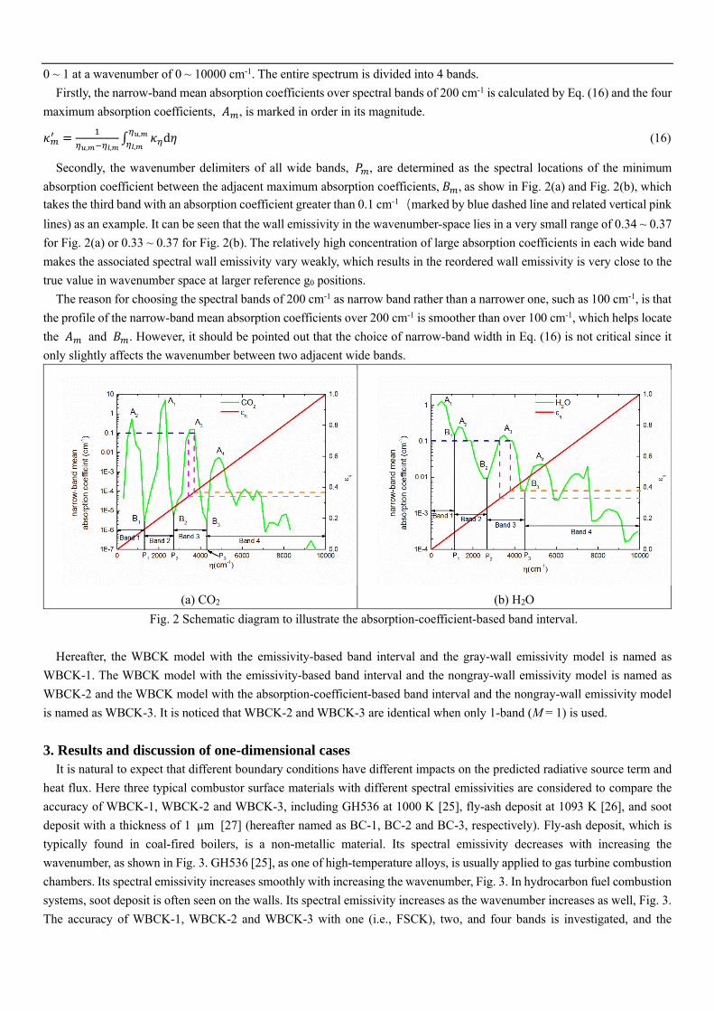
0 ~ 1 at a wavenumber of 0 ~ 10000 cm-1. The entire spectrum is divided into 4 bands.

Firstly, the narrow-band mean absorption coefficients over spectral bands of 200 cm-1 is calculated by Eq. (16) and the four

maximum absorption coefficients, 𝐴𝑚, is marked in order in its magnitude.

𝜅𝑚′ =

1

𝜂𝑢,𝑚−𝜂𝑙,𝑚∫ 𝜅𝜂d𝜂𝜂𝑢,𝑚𝜂𝑙,𝑚

(16)

Secondly, the wavenumber delimiters of all wide bands, 𝑃𝑚, are determined as the spectral locations of the minimum

absorption coefficient between the adjacent maximum absorption coefficients, 𝐵𝑚, as show in Fig. 2(a) and Fig. 2(b), which

takes the third band with an absorption coefficient greater than 0.1 cm-1（marked by blue dashed line and related vertical pink

lines) as an example. It can be seen that the wall emissivity in the wavenumber-space lies in a very small range of 0.34 ~ 0.37

for Fig. 2(a) or 0.33 ~ 0.37 for Fig. 2(b). The relatively high concentration of large absorption coefficients in each wide band

makes the associated spectral wall emissivity vary weakly, which results in the reordered wall emissivity is very close to the

true value in wavenumber space at larger reference g0 positions.

The reason for choosing the spectral bands of 200 cm-1 as narrow band rather than a narrower one, such as 100 cm-1, is that

the profile of the narrow-band mean absorption coefficients over 200 cm-1 is smoother than over 100 cm-1, which helps locate

the 𝐴𝑚 and 𝐵𝑚. However, it should be pointed out that the choice of narrow-band width in Eq. (16) is not critical since it

only slightly affects the wavenumber between two adjacent wide bands.

(a) CO2

(b) H2O

Fig. 2 Schematic diagram to illustrate the absorption-coefficient-based band interval.

Hereafter, the WBCK model with the emissivity-based band interval and the gray-wall emissivity model is named as

WBCK-1. The WBCK model with the emissivity-based band interval and the nongray-wall emissivity model is named as

WBCK-2 and the WBCK model with the absorption-coefficient-based band interval and the nongray-wall emissivity model

is named as WBCK-3. It is noticed that WBCK-2 and WBCK-3 are identical when only 1-band (M = 1) is used.

3. Results and discussion of one-dimensional cases

It is natural to expect that different boundary conditions have different impacts on the predicted radiative source term and

heat flux. Here three typical combustor surface materials with different spectral emissivities are considered to compare the

accuracy of WBCK-1, WBCK-2 and WBCK-3, including GH536 at 1000 K [25], fly-ash deposit at 1093 K [26], and soot

deposit with a thickness of 1 μm [27] (hereafter named as BC-1, BC-2 and BC-3, respectively). Fly-ash deposit, which is

typically found in coal-fired boilers, is a non-metallic material. Its spectral emissivity decreases with increasing the

wavenumber, as shown in Fig. 3. GH536 [25], as one of high-temperature alloys, is usually applied to gas turbine combustion

chambers. Its spectral emissivity increases smoothly with increasing the wavenumber, Fig. 3. In hydrocarbon fuel combustion

systems, soot deposit is often seen on the walls. Its spectral emissivity increases as the wavenumber increases as well, Fig. 3.

The accuracy of WBCK-1, WBCK-2 and WBCK-3 with one (i.e., FSCK), two, and four bands is investigated, and the

influence of the number of bands will also be discussed later.

Fig. 3 The spectral emissivity of fly-ash deposit at 1093 K [26], GH536 at 1000 K [25], and soot deposit with a thickness

of 1 μm [27].

In this section, three one-dimensional isothermal and homogeneous cases are investigated, which includes a pure CO2 case,

a pure H2O case, and a CO2-H2O mixture case, as shown in Table 1. The discrete-ordinates method (DOM) along with the S8

angular discretization scheme [14] is used to solve RTE. The spectral absorption coefficients of radiating gases are derived

from the HITEMP 2010 database [29] and the HAPI code [30]. The range of wavenumber covers from 200 𝑐𝑚−1 to 10000

𝑐𝑚−1 and the wavenumber interval is set to 0.02 𝑐𝑚−1 in LBL calculations, which has been proven to be a good

compromise between accuracy and efficiency [15]. The 32-point Gauss-Chebyshev scheme is selected to reduce the error

induced by quadrature scheme. For both the gray and non-gray boundary conditions, iteration is necessary in solving the RTEs

due to reflection of incident radiative heat flux at walls. The convergence condition for all the bands is

𝑚𝑎𝑥 (𝐺𝑚𝑄−𝐺𝑚

𝑄−1

𝐺𝑚𝑄 ) < 10−6 (17)

where Q is the number of iterations and Gm is incident radiation of the mth band evaluated as

𝐺𝑚𝑄 = ∑ ∑ 𝑤𝑛𝑢𝑗𝐼𝑔0,𝑚,𝑛,𝑗

𝐽𝑗=1

𝑁𝑛=1 (18)

where 𝑢𝑗 is weight of the jth ordinate and J is the number of angular ordinates.

Table 1. Description of the thermal conditions in the three one-dimensional cases.

Case Number of

subcases

Length L

(m)

Internal

temperature (K)

Wall temperature

(K)

𝑥𝐶𝑂2 𝑥𝐻2𝑂 Boundary

condition

(a) BC-1

1 (b) 1 2500 300 - 2000 0.1 0 BC-2

(c) BC-3

(a) BC-1

2 (b) 1 2500 300 - 2000 0 0.1 BC-2

(c) BC-3

(a) BC-1

3 (b) 1 2500 300 - 2000 0.1 0.2 BC-2

(c) BC-3

Three metrics are used to evaluate the accuracy of the three WBCK models, including the local relative error of radiative

source term (LE(x)), the total absolute relative error of radiative source term (TE), and the error of heat flux at the right wall

(EF). These quantities are defined as:

LE(x) = −𝛁∙�̇�𝑅

′′𝐹𝑆𝐶𝐾 𝑜𝑟 𝑊𝐵𝐶𝐾

(𝑥) + 𝛁∙�̇�𝑅′′𝐿𝐵𝐿

(𝑥)

|𝛁∙�̇�𝑅′′𝐿𝐵𝐿

(𝑥)|𝑚𝑎𝑥

100% (19)

TE = ∫ |−𝛁 ∙ �̇�𝑅′′𝐹𝑆𝐶𝐾 𝑜𝑟 𝑊𝐵𝐶𝐾

(𝑥) + 𝛁 ∙ �̇�𝑅′′𝐿𝐵𝐿(𝑥)|𝑑𝑥

𝐿

0/ ∫ |𝛁 ∙ �̇�𝑅

′′𝐿𝐵𝐿(𝑥)|

𝐿

0𝑑𝑥 (20)

EF = (�̇�𝑅′′𝐹𝑆𝐶𝐾 𝑜𝑟 𝑊𝐵𝐶𝐾

(𝐿) − �̇�𝑅′′𝐿𝐵𝐿(𝐿))/�̇�𝑅

′′𝐿𝐵𝐿(𝐿) (21)

where L is the length of computational domain.

3.1 The pure CO2 case

Firstly, a pure CO2 case (Case 1) is considered, as shown in Table 1. The gaseous medium bounded by the two walls consists

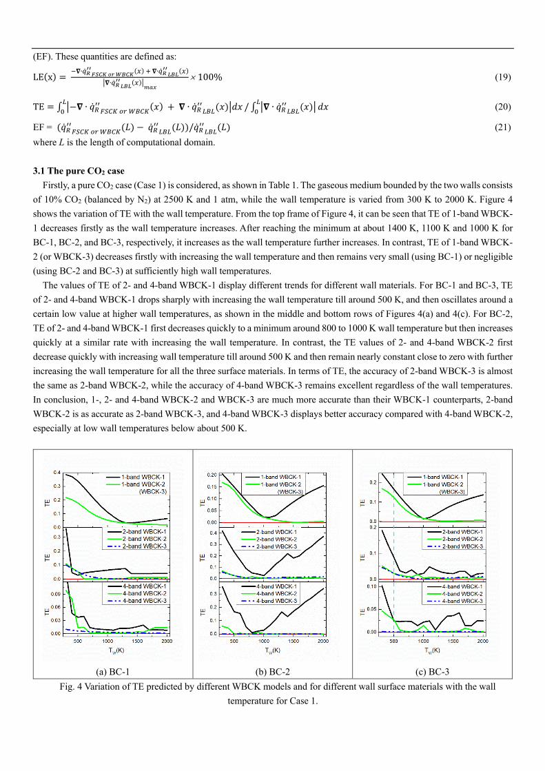
of 10% CO2 (balanced by N2) at 2500 K and 1 atm, while the wall temperature is varied from 300 K to 2000 K. Figure 4

shows the variation of TE with the wall temperature. From the top frame of Figure 4, it can be seen that TE of 1-band WBCK-

1 decreases firstly as the wall temperature increases. After reaching the minimum at about 1400 K, 1100 K and 1000 K for

BC-1, BC-2, and BC-3, respectively, it increases as the wall temperature further increases. In contrast, TE of 1-band WBCK-

2 (or WBCK-3) decreases firstly with increasing the wall temperature and then remains very small (using BC-1) or negligible

(using BC-2 and BC-3) at sufficiently high wall temperatures.

The values of TE of 2- and 4-band WBCK-1 display different trends for different wall materials. For BC-1 and BC-3, TE

of 2- and 4-band WBCK-1 drops sharply with increasing the wall temperature till around 500 K, and then oscillates around a

certain low value at higher wall temperatures, as shown in the middle and bottom rows of Figures 4(a) and 4(c). For BC-2,

TE of 2- and 4-band WBCK-1 first decreases quickly to a minimum around 800 to 1000 K wall temperature but then increases

quickly at a similar rate with increasing the wall temperature. In contrast, the TE values of 2- and 4-band WBCK-2 first

decrease quickly with increasing wall temperature till around 500 K and then remain nearly constant close to zero with further

increasing the wall temperature for all the three surface materials. In terms of TE, the accuracy of 2-band WBCK-3 is almost

the same as 2-band WBCK-2, while the accuracy of 4-band WBCK-3 remains excellent regardless of the wall temperatures.

In conclusion, 1-, 2- and 4-band WBCK-2 and WBCK-3 are much more accurate than their WBCK-1 counterparts, 2-band

WBCK-2 is as accurate as 2-band WBCK-3, and 4-band WBCK-3 displays better accuracy compared with 4-band WBCK-2,

especially at low wall temperatures below about 500 K.

(a) BC-1

(b) BC-2

(c) BC-3

Fig. 4 Variation of TE predicted by different WBCK models and for different wall surface materials with the wall

temperature for Case 1.

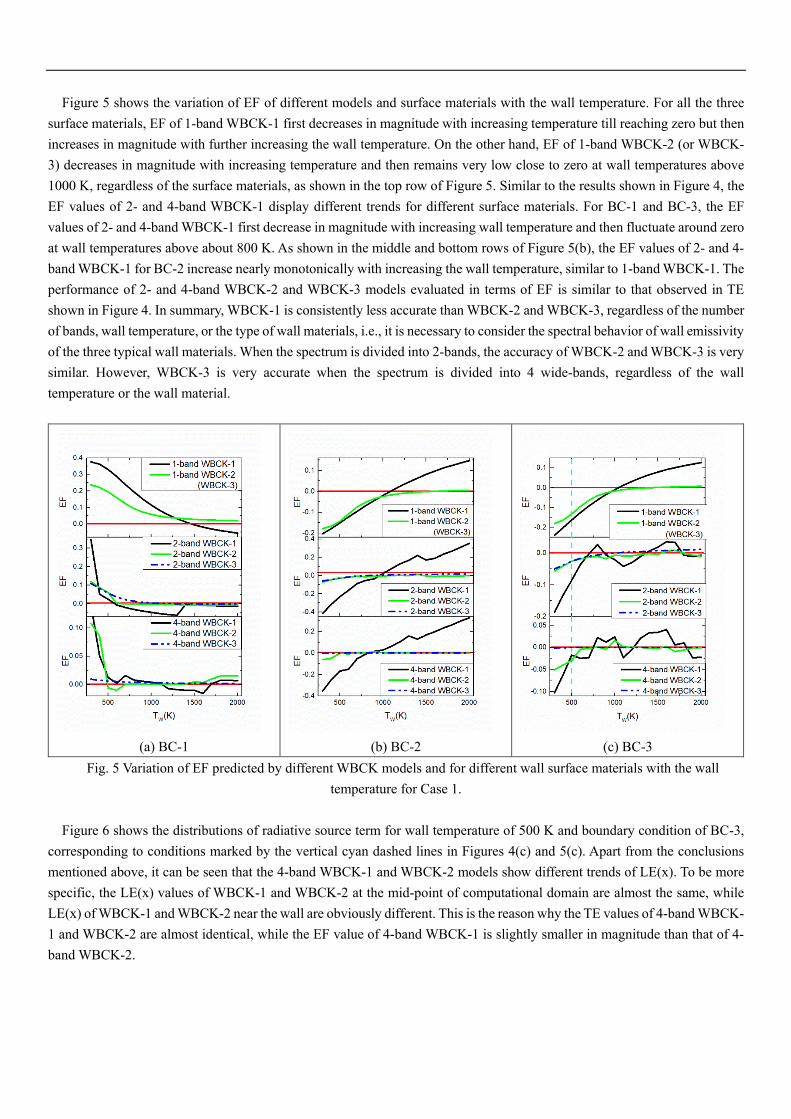
Figure 5 shows the variation of EF of different models and surface materials with the wall temperature. For all the three

surface materials, EF of 1-band WBCK-1 first decreases in magnitude with increasing temperature till reaching zero but then

increases in magnitude with further increasing the wall temperature. On the other hand, EF of 1-band WBCK-2 (or WBCK-

3) decreases in magnitude with increasing temperature and then remains very low close to zero at wall temperatures above

1000 K, regardless of the surface materials, as shown in the top row of Figure 5. Similar to the results shown in Figure 4, the

EF values of 2- and 4-band WBCK-1 display different trends for different surface materials. For BC-1 and BC-3, the EF

values of 2- and 4-band WBCK-1 first decrease in magnitude with increasing wall temperature and then fluctuate around zero

at wall temperatures above about 800 K. As shown in the middle and bottom rows of Figure 5(b), the EF values of 2- and 4-

band WBCK-1 for BC-2 increase nearly monotonically with increasing the wall temperature, similar to 1-band WBCK-1. The

performance of 2- and 4-band WBCK-2 and WBCK-3 models evaluated in terms of EF is similar to that observed in TE

shown in Figure 4. In summary, WBCK-1 is consistently less accurate than WBCK-2 and WBCK-3, regardless of the number

of bands, wall temperature, or the type of wall materials, i.e., it is necessary to consider the spectral behavior of wall emissivity

of the three typical wall materials. When the spectrum is divided into 2-bands, the accuracy of WBCK-2 and WBCK-3 is very

similar. However, WBCK-3 is very accurate when the spectrum is divided into 4 wide-bands, regardless of the wall

temperature or the wall material.

(a) BC-1

(b) BC-2

(c) BC-3

Fig. 5 Variation of EF predicted by different WBCK models and for different wall surface materials with the wall

temperature for Case 1.

Figure 6 shows the distributions of radiative source term for wall temperature of 500 K and boundary condition of BC-3,

corresponding to conditions marked by the vertical cyan dashed lines in Figures 4(c) and 5(c). Apart from the conclusions

mentioned above, it can be seen that the 4-band WBCK-1 and WBCK-2 models show different trends of LE(x). To be more

specific, the LE(x) values of WBCK-1 and WBCK-2 at the mid-point of computational domain are almost the same, while

LE(x) of WBCK-1 and WBCK-2 near the wall are obviously different. This is the reason why the TE values of 4-band WBCK-

1 and WBCK-2 are almost identical, while the EF value of 4-band WBCK-1 is slightly smaller in magnitude than that of 4-

band WBCK-2.

(a) 1-band WBCK

(b) 2-bands WBCK

(c) 4-bands WBCK

Fig. 6 Distributions of the radiative source term of Case 1 for 500 K wall temperature with BC-3 as the boundary

material.

To explain why WBCK-2 is more accurate than WBCK-1, the left frame of Fig. 7 displays the 2nd-band spectral absorption

coefficient of 2-band WBCK-1, the normalized spectral Planck function, 𝐼𝑏𝜂/𝐼𝑏 (Tw = 500 K), and the spectral emissivity of

BC-3 as a function of wavenumber. The right frame of Fig. 7 shows the reordered absorption coefficient, 𝑘∗, and the 2nd-

band reordered emissivity of WBCK-1 and WBCK-2 as a function of 𝑔0. As is known, larger absorption coefficients are in

general more important than smaller ones in radiative heat transfer, as shown in WBCK RTE (Eq. (4)). The spectral absorption

coefficients of CO2 at the 4.3 μm band (i.e., centered at 2410 cm-1) are much larger than those at other spectral positions

[14], which means that the spectral emissivity near 2410 cm-1 has a great impact on the predicted radiative heat transfer. The

gray horizontal dashed line marks the absorption coefficients larger than 0.05 cm-1 (𝜅 for the wavenumber-space and k* for

the g0-space). The cyan horizontal dashed lines mark the corresponding range of spectral emissivity, which is from 0.62 to

0.65 (see the left frame of Figure 7). The emissivity of WBCK-2 for absorption coefficients larger than 0.05 cm-1 is between

0.62 and 0.64, and very close to the spectral emissivity in the wavenumber-space. As for WBCK-1, the emissivity of WBCK-

1 is 0.59 due to the influence of spectral Planck function weighting (see the red line of left frame of Figure 7). In other words,

the emissivity of WBCK-2 is more accurate than that of WBCK-1, resulting in better accuracy of WBCK-2 than WBCK-1.

Fig. 7 The prediction of 2nd-band emissivity of two-band WBCK-1 and WBCK-2. The left frame displays the 2nd-band

spectral absorption coefficient, the spectral Planck function and the spectral emissivity of BC-3. The right frame shows the

reordered absorption coefficient and the 2nd-band emissivity of WBCK-1 and WBCK-2.

Furthermore, from Fig. 6(c), it can be found that LE(x) of 4-band WBCK-3 is negligible, while LE(x) of 4-band WBCK-2

remains nearly constant around 1%. This is attributed to the different band intervals of WBCK-2 and WBCK-3. For WBCK-

2, the four bands are 200-900 cm-1, 900-1400 cm-1, 1400-2000 cm-1 and 2000-10000 cm-1, while for WBCK-3, the four bands

are 200-1300 cm-1, 1300-2700 cm-1, 2700-4300 cm-1 and 4300-10000 cm-1.

Figure 8 displays the 4th-band emissivity of 4-band WBCK-2. The gray horizontal dashed lines mark absorption

coefficients that lie between 0.001 cm-1 and 0.01 cm-1, and the cyan horizontal dashed line indicate the spectral emissivity of

BC-3 (between 0.75 and 0.78, see the left frame of Figure 8). However, the emissivity predicted by WBCK-2 is around 0.69,

and is much smaller than the spectral emissivity in the wavenumber-space. Figure 9 shows the 3rd-band emissivity of 4-band

WBCK-3. The emissivity of WBCK-3 ranges from 0.75 to 0.77. In other words, the reordered emissivity predicted by WBCK-

3 shows better agreement with the spectral emissivity in the wavenumber-space than it predicted by WBCK-2. This explains

why WBCK-3 is more accurate than WBCK-2 at a low wall temperature.

Fig. 8 The prediction of 4th-band emissivity of 4-band WBCK-1 and WBCK-2. The left frame displays the 4th-band

spectral absorption coefficient and the spectral emissivity of BC-3. The right frame shows the reordered absorption

coefficient and the 4th-band emissivity of WBCK-1 and WBCK-2.

Fig. 9 The prediction of 3rd-band emissivity of 4-band WBCK-3. The left frame displays the 3rd-band spectral absorption

coefficient and the spectral emissivity of BC-3. The right frame illustrates the reordered absorption coefficient and the 3rd-

band emissivity of WBCK-3.

3.2 The pure H2O case

The second test case (Case 2) contains pure H2O as the radiating gas, whose thermal conditions are given Table 1. The

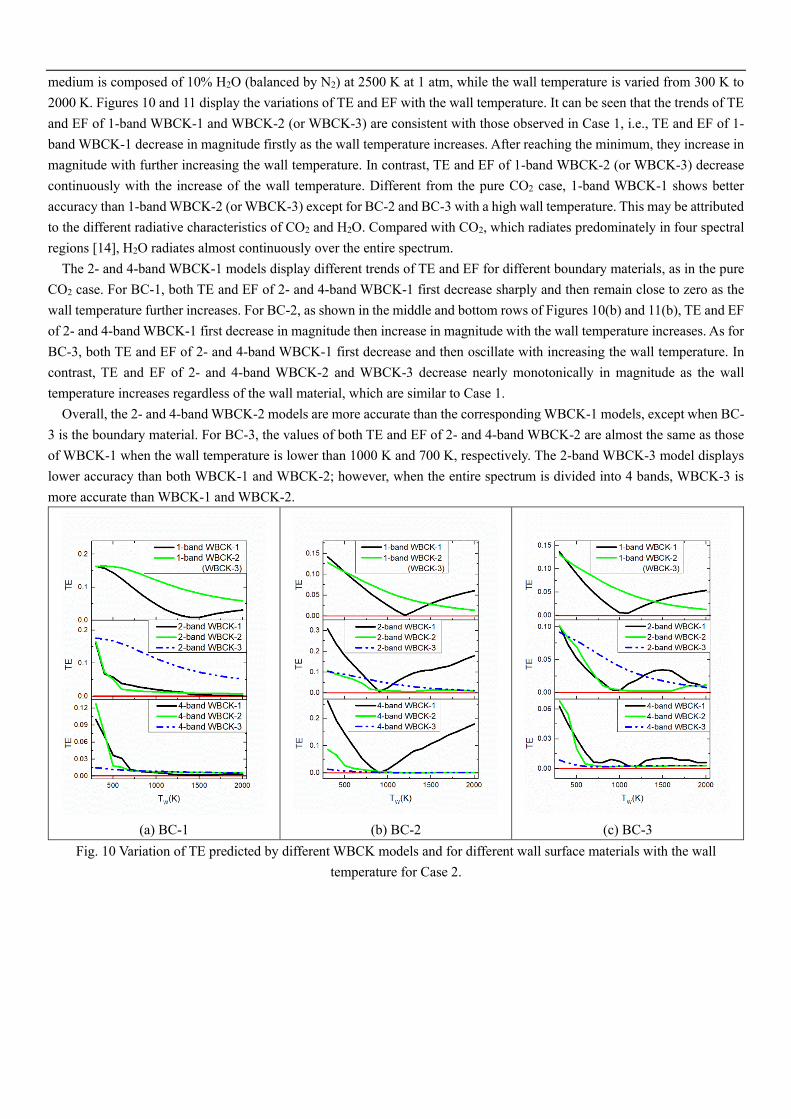
medium is composed of 10% H2O (balanced by N2) at 2500 K at 1 atm, while the wall temperature is varied from 300 K to

2000 K. Figures 10 and 11 display the variations of TE and EF with the wall temperature. It can be seen that the trends of TE

and EF of 1-band WBCK-1 and WBCK-2 (or WBCK-3) are consistent with those observed in Case 1, i.e., TE and EF of 1-

band WBCK-1 decrease in magnitude firstly as the wall temperature increases. After reaching the minimum, they increase in

magnitude with further increasing the wall temperature. In contrast, TE and EF of 1-band WBCK-2 (or WBCK-3) decrease

continuously with the increase of the wall temperature. Different from the pure CO2 case, 1-band WBCK-1 shows better

accuracy than 1-band WBCK-2 (or WBCK-3) except for BC-2 and BC-3 with a high wall temperature. This may be attributed

to the different radiative characteristics of CO2 and H2O. Compared with CO2, which radiates predominately in four spectral

regions [14], H2O radiates almost continuously over the entire spectrum.

The 2- and 4-band WBCK-1 models display different trends of TE and EF for different boundary materials, as in the pure

CO2 case. For BC-1, both TE and EF of 2- and 4-band WBCK-1 first decrease sharply and then remain close to zero as the

wall temperature further increases. For BC-2, as shown in the middle and bottom rows of Figures 10(b) and 11(b), TE and EF

of 2- and 4-band WBCK-1 first decrease in magnitude then increase in magnitude with the wall temperature increases. As for

BC-3, both TE and EF of 2- and 4-band WBCK-1 first decrease and then oscillate with increasing the wall temperature. In

contrast, TE and EF of 2- and 4-band WBCK-2 and WBCK-3 decrease nearly monotonically in magnitude as the wall

temperature increases regardless of the wall material, which are similar to Case 1.

Overall, the 2- and 4-band WBCK-2 models are more accurate than the corresponding WBCK-1 models, except when BC-

3 is the boundary material. For BC-3, the values of both TE and EF of 2- and 4-band WBCK-2 are almost the same as those

of WBCK-1 when the wall temperature is lower than 1000 K and 700 K, respectively. The 2-band WBCK-3 model displays

lower accuracy than both WBCK-1 and WBCK-2; however, when the entire spectrum is divided into 4 bands, WBCK-3 is

more accurate than WBCK-1 and WBCK-2.

(a) BC-1

(b) BC-2

(c) BC-3

Fig. 10 Variation of TE predicted by different WBCK models and for different wall surface materials with the wall

temperature for Case 2.

(a) BC-1

(b) BC-2

(c) BC-3

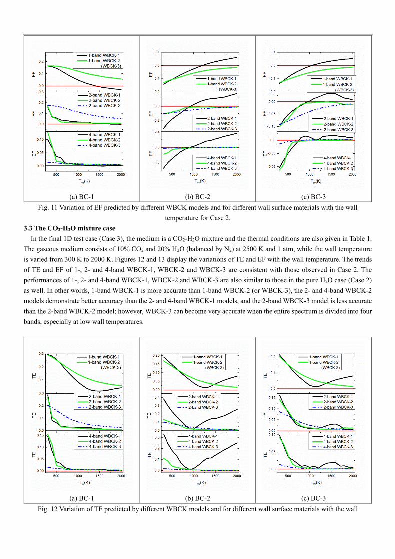
Fig. 11 Variation of EF predicted by different WBCK models and for different wall surface materials with the wall

temperature for Case 2.

3.3 The CO2-H2O mixture case

In the final 1D test case (Case 3), the medium is a CO2-H2O mixture and the thermal conditions are also given in Table 1.

The gaseous medium consists of 10% CO2 and 20% H2O (balanced by N2) at 2500 K and 1 atm, while the wall temperature

is varied from 300 K to 2000 K. Figures 12 and 13 display the variations of TE and EF with the wall temperature. The trends

of TE and EF of 1-, 2- and 4-band WBCK-1, WBCK-2 and WBCK-3 are consistent with those observed in Case 2. The

performances of 1-, 2- and 4-band WBCK-1, WBCK-2 and WBCK-3 are also similar to those in the pure H2O case (Case 2)

as well. In other words, 1-band WBCK-1 is more accurate than 1-band WBCK-2 (or WBCK-3), the 2- and 4-band WBCK-2

models demonstrate better accuracy than the 2- and 4-band WBCK-1 models, and the 2-band WBCK-3 model is less accurate

than the 2-band WBCK-2 model; however, WBCK-3 can become very accurate when the entire spectrum is divided into four

bands, especially at low wall temperatures.

(a) BC-1

(b) BC-2

(c) BC-3

Fig. 12 Variation of TE predicted by different WBCK models and for different wall surface materials with the wall

temperature for Case 3.

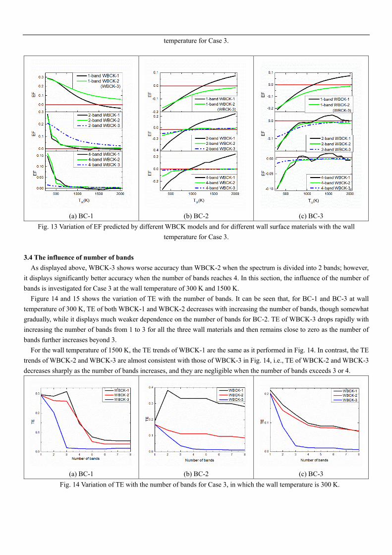
(a) BC-1

(b) BC-2

(c) BC-3

Fig. 13 Variation of EF predicted by different WBCK models and for different wall surface materials with the wall

temperature for Case 3.

3.4 The influence of number of bands

As displayed above, WBCK-3 shows worse accuracy than WBCK-2 when the spectrum is divided into 2 bands; however,

it displays significantly better accuracy when the number of bands reaches 4. In this section, the influence of the number of

bands is investigated for Case 3 at the wall temperature of 300 K and 1500 K.

Figure 14 and 15 shows the variation of TE with the number of bands. It can be seen that, for BC-1 and BC-3 at wall

temperature of 300 K, TE of both WBCK-1 and WBCK-2 decreases with increasing the number of bands, though somewhat

gradually, while it displays much weaker dependence on the number of bands for BC-2. TE of WBCK-3 drops rapidly with

increasing the number of bands from 1 to 3 for all the three wall materials and then remains close to zero as the number of

bands further increases beyond 3.

For the wall temperature of 1500 K, the TE trends of WBCK-1 are the same as it performed in Fig. 14. In contrast, the TE

trends of WBCK-2 and WBCK-3 are almost consistent with those of WBCK-3 in Fig. 14, i.e., TE of WBCK-2 and WBCK-3

decreases sharply as the number of bands increases, and they are negligible when the number of bands exceeds 3 or 4.

(a) BC-1

(b) BC-2

(c) BC-3

Fig. 14 Variation of TE with the number of bands for Case 3, in which the wall temperature is 300 K.

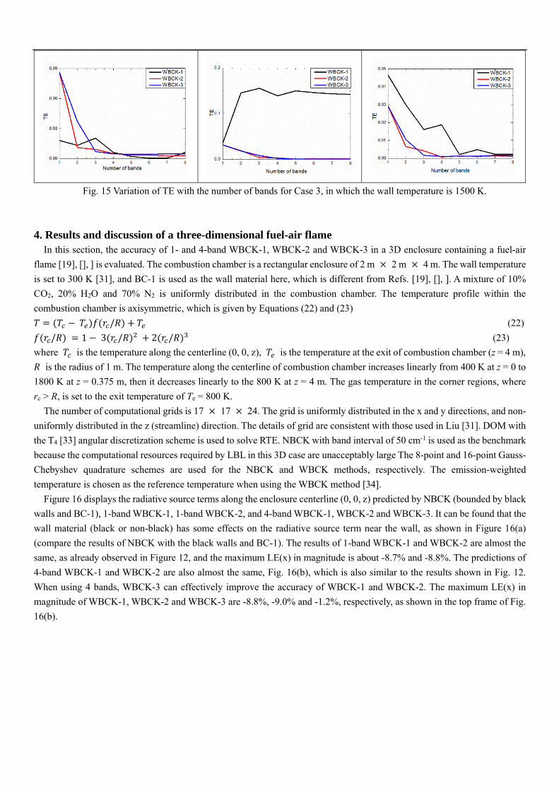
Fig. 15 Variation of TE with the number of bands for Case 3, in which the wall temperature is 1500 K.

4. Results and discussion of a three-dimensional fuel-air flame

In this section, the accuracy of 1- and 4-band WBCK-1, WBCK-2 and WBCK-3 in a 3D enclosure containing a fuel-air

flame [19], [], ] is evaluated. The combustion chamber is a rectangular enclosure of 2 m × 2 m × 4 m. The wall temperature

is set to 300 K [31], and BC-1 is used as the wall material here, which is different from Refs. [19], [], ]. A mixture of 10%

CO2, 20% H2O and 70% N2 is uniformly distributed in the combustion chamber. The temperature profile within the

combustion chamber is axisymmetric, which is given by Equations (22) and (23)

𝑇 = (𝑇𝑐 − 𝑇𝑒)𝑓(𝑟𝑐/𝑅) + 𝑇𝑒 (22)

𝑓(𝑟𝑐/𝑅) = 1 − 3(𝑟𝑐/𝑅)2 + 2(𝑟𝑐/𝑅)

3 (23)

where 𝑇𝑐 is the temperature along the centerline (0, 0, z), 𝑇𝑒 is the temperature at the exit of combustion chamber (z = 4 m),

𝑅 is the radius of 1 m. The temperature along the centerline of combustion chamber increases linearly from 400 K at z = 0 to

1800 K at z = 0.375 m, then it decreases linearly to the 800 K at z = 4 m. The gas temperature in the corner regions, where

rc > R, is set to the exit temperature of Te = 800 K.

The number of computational grids is 17 × 17 × 24. The grid is uniformly distributed in the x and y directions, and non-

uniformly distributed in the z (streamline) direction. The details of grid are consistent with those used in Liu [31]. DOM with

the T4 [33] angular discretization scheme is used to solve RTE. NBCK with band interval of 50 cm-1 is used as the benchmark

because the computational resources required by LBL in this 3D case are unacceptably large The 8-point and 16-point Gauss-

Chebyshev quadrature schemes are used for the NBCK and WBCK methods, respectively. The emission-weighted

temperature is chosen as the reference temperature when using the WBCK method [34].

Figure 16 displays the radiative source terms along the enclosure centerline (0, 0, z) predicted by NBCK (bounded by black

walls and BC-1), 1-band WBCK-1, 1-band WBCK-2, and 4-band WBCK-1, WBCK-2 and WBCK-3. It can be found that the

wall material (black or non-black) has some effects on the radiative source term near the wall, as shown in Figure 16(a)

(compare the results of NBCK with the black walls and BC-1). The results of 1-band WBCK-1 and WBCK-2 are almost the

same, as already observed in Figure 12, and the maximum LE(x) in magnitude is about -8.7% and -8.8%. The predictions of

4-band WBCK-1 and WBCK-2 are also almost the same, Fig. 16(b), which is also similar to the results shown in Fig. 12.

When using 4 bands, WBCK-3 can effectively improve the accuracy of WBCK-1 and WBCK-2. The maximum LE(x) in

magnitude of WBCK-1, WBCK-2 and WBCK-3 are -8.8%, -9.0% and -1.2%, respectively, as shown in the top frame of Fig.

16(b).

(a)

(b)

Fig. 16 The radiative source term distributions along the enclosure centerline (0, 0, z) of the fuel-air flame predicted by

NBCK (bounded by the black walls and BC-1), 1-band WBCK-1, 1-band WBCK-2, and 4-band WBCK-1, WBCK-2 and

WBCK-3.

Figure 17 displays the net heat fluxes along the centerline of a side wall, (1 m, 1 m, z), by NBCK (bounded by the black

walls and BC-1), 1-band WBCK-1, 1-band WBCK-2, and 4-band WBCK-1, WBCK-2 and WBCK-3. There are obvious

discrepancies between the NBCK results for the two boundary conditions (black wall vs. BC-1). For the black walls, the

maximum flux along the line of (1 m, 1 m, z) is 20.5 kw/m2, which is consistent with the result of Porter et al. [32], while for

BC-1, the maximum net flux is lower at 16.1 kw/m2. Similar to the radiative source term along the center line (0, 0, z), 1-band

WBCK-1 and WBCK-2 predicted undistinguishable results but with large errors. When using 4 bands, WBCK-1 and WBCK-

2 yield significantly better accuracy than their 1-band counterparts and their results are very close to each other as well. When

the spectrum is divided into 4 bands, WBCK-3 offers the best accuracy among the three WBCK models investigated.

Fig. 17 The radiative heat flux along the line of (1 m, 1 m, z) predicted by NBCK (bounded by the black walls and BC-1),

1-band WBCK-1, 1-band WBCK-2, and 4-band WBCK-1, WBCK-2 and WBCK-3.

5. Conclusions

In this work, a nongray-wall emissivity model is proposed within the framework of the Wide-Band Correlated K-

distribution method. In addition, an absorption-coefficient-based strategy is developed to optimize the band intervals. Three

1D isothermal and homogeneous cases bounded by the fly-ash deposit, GH536, and soot deposit and a 3D fuel-air flame

bounded by a rectangular enclosure bounded by fly-ash deposit coated walls are considered as test cases to evaluate the

accuracy of WBCK-1, WBCK-2 and WBCK-3 for different numbers of bands up to 4 in the prediction of radiative heat

transfer. The LBL and NBCK results are obtained and used as the benchmarks in the one- and three-dimensional cases,

respectively. The following conclusions can be drawn from this work:

(1) WBCK-2 improves the accuracy of WBCK-1 when the number of bands is larger than 1. For 1-band WBCK (i.e.,

FSCK), WBCK-2 is more accurate than WBCK-1 in the pure CO2 case, while they show the opposite trends in the pure H2O

and CO2-H2O case.

(2) When the entire spectrum is divided into 2 bands, WBCK-3 demonstrates the worst accuracy among the models and

thermal conditions investigated.

(3) When the spectrum is divided into 4 bands, WBCK-3 is more accurate than WBCK-1 and WBCK-2 for low-temperature

wall. For high-temperature wall, both WBCK-2 and WBCK-3 agree well with the benchmark.

(4) For the three types of typical wall material of nongray emissivity encountered in practical combustion systems, it is

sufficient to divide the entire spectrum into 3 or 4 bands when using WBCK-3 for accurate predictions of radiative heat

transfer.

Acknowledgments

The authors are grateful for the former support of “National Natural Science Foundation of China ”(Grant No.50606004 )

on the radiative heat transfer modelling topic, and the support of “Overseas Expertise Introduction Project for Discipline

Innovation ”(111 project, Grant No. B08009 ) for international academic exchanges.

Reference

[1] Modest M F, Haworth D C. Radiative heat transfer in turbulent combustion systems: theory and application. New York:

Springer; 2016.

[2] Wall T F, Bhattacharya S P, Baxter L L, Richards G, Harb J N. The character of ash deposits and the thermal performance

of furnaces. Fuel Process Technol 1995; 44(1): 143-153.

[3] Dannecker R, Schildmacher K U, Noll B, Koch R, Hase M, Krebs W, Aigner M. Impact of radiation on the wall heat

load at a test bench gas turbine combustion chamber: measurements and CFD simulation. ASME Turbo Expo 2007; 4:

1311-1321.

[4] Ren T, Modest M F, Roy S. Monte carlo simulation for radiative transfer in a high-pressure industrial gas turbine

combustion chamber. J Eng Gas Turb Power 2018; 140(5): 051503.

[5] Goody R M. A statistical model for water-vapor absorption, Quart J R Meteorol Soc 1952; 78: 165-169.

[6] Malkmus W. Random Lorentz band model with exponential-tailed S-1 line-intensity distribution function. J Opt Soc Am

1967; 57: 323-329.

[7] Lacis A A, Oinas V. A description of the correlated k distribution method for modeling non-gray gaseous absorption,

thermal emission, and multiple scattering in vertically inhomogeneous atmospheres. J Geophys Res 1991; 96: 9027-

9063.

[8] Modest M F, Narrow-band and full-spectrum k-distributions for radiative heat transfer—correlated-k vs. scaling

approximation. J Quant Spectrosc Radiat Transf 2003; 76: 69-83.

[9] Ströhle J, Coelho P J. On the application of the exponential wide band model to the calculation of radiative heat transfer

in one- and two-dimensional enclosures. Intl J Heat Mass Transf 2002; 45(10): 2129-2139.

[10] Ströhle J. Assessment of the re-ordered wide band model for non-grey radiative transfer calculations in 3D enclosures. J

Quant Spectrosc Radiat Transf 2008; 109(9): 1622-1640.

[11] Denison M K, Webb B W. A spectral line-based weighted sum of gray gases model for arbitrary RTE solvers. ASME J

Heat Transf 1993; 115(4): 1004-1012.

[12] Pierrot L, Rivière P, Soufiani A, Taine J. A fictitious-gas-based absorption distribution function global model for radiative

transfer in hot gases. J Quant Spectrosc Radiat Transf 1999; 62(5): 609-624.

[13] Johansson R, Leckner B, Andersson K, Johnsson F. Account for variations in the H2O to CO2 molar ratio when modelling

gaseous radiative heat transfer with the Weighted-Sum-of-Grey-Gases Model. Combust Flame 2011; 158(5): 893-901.

[14] Modest M F. Radiative heat transfer. 3rd ed.. New York: Academic Press; 2013.

[15] Chu H, Ren F, Feng Y, Gu M, Zheng S. A comprehensive evaluation of the non gray gas thermal radiation using the line-

by-line model in one- and two-dimensional enclosures. Appl Therm Eng 2017; 124: 362-370.

[16] Solovjov V P, Lemonnier D, Webb B W. Efficient cumulative wavenumber model of radiative transfer in gaseous media

bounded by non-gray walls. J Quant Spectrosc Radiat Transf 2013; 128: 2-9.

[17] Fonseca R J C, Fraga G C, Silva R B, Franca F H R. Application of the WSGG model to solve the radiative transfer in

gaseous systems with nongray boundaries. ASME J Heat Transf 2018; 140(5): 052701.

[18] Bordbar H, Hyppänen T. Line by line based band identification for non-gray gas modeling with a banded approach. Int

J Heat Mass Tran 2018; 127: 870-884.

[19] Bordbar H, Maximov A, Hyppänen T. Improved banded method for spectral thermal radiation in participating media

with spectrally dependent wall emittance. Appl Energ 2019; 235: 1090-1105.

[20] Fonseca R J C, Fraga G C, Franca F H R. A simplified approach to compute the radiative transfer in a participating media

bounded by non-gray walls. Eurotherm Seminar 110-Computational Thermal Radiation in Participating Media-VI; 2018.

[21] Liu Y, Liu G, Hu H, Kong B. A wavenumber subinterval grouping strategy compatible with non-gray metal wall

boundaries used in multi-scale multi-group full spectrum k-distribution gas radiation model. Appl Therm Eng 2019; 113:

20-26.

[22] Zhao X Y, Haworth D C, Ren T, Modest M F. A transported probability density function/photon Monte Carlo method for

high-temperature oxy-natural gas combustion with spectral gas and wall radiation. Combust Theor Model 2013; 17(2):

354-381.

[23] Yang X, He Z, Dong S, Tan H. Prediction of turbulence radiation interactions of CH2-H2/air turbulent flames as

atmospheric and elevated pressures. Int J Hydrogen Energ 2018; 43(32): 15537-15550.

[24] Johansson R, Leckner B, Andersson K, Johnsson F. Influence of particle and gas radiation in oxy-fuel combustion. Int J

Heat Mass Tran 2013; 65: 143-152.

[25] Kong B, Li T, Eri Q. Normal spectral emissivity of GH536 (HastelloyX) in three surface conditions. Appl Therm Eng

2017; 113: 20-26.

[26] Markham J L, Best P E, Solomon P R, Yu Z Z. Measurement of radiative properties of ash and slag by FT-IR emission

and reflection spectroscopy. ASME J Heat Transf 1992; 114(2): 458-64.

[27] Liebert C H, Hibbard R R. Spectral emittance of soot. NASA Technical Notes 1970;

[28] Hu H, Wang Q. Improved spectral absorption coefficient grouping strategy of wide band k-distribution model used for

calculation of infrared remote sensing signal oh hot exhaust systems. J Quant Spectrosc Radiat Transf 2018; 213: 17-34.

[29] Rothman L S, Gordon I E, Barber R J, Dothe H, Gamache R R, Goldman A, Perevalov V I, Tashkun S A, Gamache J.

HITEMP, the high-temperature molecular spectroscopic database. J Quant Spectros Radiat Transf 2010; 111: 2139-2150.

[30] Kochanov R V, Gordon I E, Rothman L S, Wcislo P, Hill C, Wilzewski J S. HITRAN application programming interface

(HAPI): a comprehensive approach to working with spectroscopic data. J Quant Spectrosc Radiat Transf 2016; 177: 15-

30.

[31] Liu F. Numerical solutions of three-dimensional non-grey gas radiative transfer using the statistical narrow-band model.

ASME J Heat Transfer 1999; 121(1): 200-203.

[32] Porter R, Liu F, Pourkashanian M, Williams A, Smith D. Evaluation of solution methods for radiative heat transfer in

gaseous oxy-fuel combustion environments. J Quant Spectrosc Radiat Transfer 2010; 111(14): 2084-2094.

[33] Thurgood C P, Becker H A, Pollard A. The TN quadrature set for the discrete-ordinates method. ASME J Heat Transfer

1995; 117: 1068-1070.

[34] Modest M F, Zhang H. The full-spectrum correlated-k distribution for thermal radiation from molecular gas-particulate

mixtures. ASME J Heat Transf 2002; 124(1): 30-38.