a new treatment for predicting the self-excited vibrations
TRANSCRIPT
HAL Id: hal-00338748https://hal.archives-ouvertes.fr/hal-00338748
Submitted on 26 Sep 2012
HAL is a multi-disciplinary open accessarchive for the deposit and dissemination of sci-entific research documents, whether they are pub-lished or not. The documents may come fromteaching and research institutions in France orabroad, or from public or private research centers.
L’archive ouverte pluridisciplinaire HAL, estdestinée au dépôt et à la diffusion de documentsscientifiques de niveau recherche, publiés ou non,émanant des établissements d’enseignement et derecherche français ou étrangers, des laboratoirespublics ou privés.
A new treatment for predicting the self-excitedvibrations of nonlinear systems with frictional interfaces:
The Constrained Harmonic Balance Method, withapplication to disc brake squeal
Nicolas Coudeyras, Jean-Jacques Sinou, Samuel Nacivet
To cite this version:Nicolas Coudeyras, Jean-Jacques Sinou, Samuel Nacivet. A new treatment for predicting the self-excited vibrations of nonlinear systems with frictional interfaces: The Constrained Harmonic BalanceMethod, with application to disc brake squeal. Journal of Sound and Vibration, Elsevier, 2009, 319(3-5), pp.1175-1199. �10.1016/j.jsv.2008.06.050�. �hal-00338748�

A new treatment for predicting the self-excited vibrationsofnonlinear systems with frictional interfaces: the Constrained
Harmonic Balance Method (CHBM). Application to discbrake squeal
N. Coudeyrasa,b, J-J. Sinoua and S. Nacivetb
a Laboratoire de Tribologie et Dynamique des Systemes UMR-CNRS 5513, Ecole Centrale de Lyon, 36avenue Guy de Collongue,69134 Ecully Cedex, France.
b PSA Peugeot Citroen, 18 rue des Fauvelles, 92250 La GarenneColombes, France.
Abstract
Noise brake squeal is still an issue since it generates high warranty costs for the automotive industryand irritation for customers. Key parameters must be known in order to reduce it. Stability analysis isa common way of studying nonlinear phenomena and has been widely used by the scientific and theengineering communities for solving disc brake squeal problems. This type of analysis provides areasof stability versus instability for driven parameters, thereby making it possible to define design criteria.Nevertheless, this technique does not permit obtaining thevibrating state of the brake system and non-linear methods have to be employed. Temporal integration isa well known method for computing thedynamic solution but as it is time consuming, nonlinear methods such the Harmonic Balance Methodare preferred. This paper presents a novel nonlinear methodcalled the Constrained Harmonic BalanceMethod (CHBM) that works for nonlinear systems subject to flutter instability. An additional constrain-ing based condition is proposed that omits the static equilibrium point (i.e. the trivial static solution ofthe nonlinear problem that would be obtained by applying theclassical Harmonic Balance Method), andtherefore focus on predicting both the Fourier coefficientsand the fundamental frequency of the station-ary nonlinear system.The effectiveness of the proposed nonlinear approach is illustrated by an analysis of disc brake squeal.The brake system under consideration is a reduced finite element model of a pad and a disc. Both sta-bility and nonlinear analyses are performed and the resultsare compared with a classical variable ordersolver integration algorithm.Therefore the objectives of the following paper are to present not only an extension of the HarmonicBalance Method (the Constrained Harmonic Balance Method -CHBM), but also to demonstrate an ap-plication to the specific problem of disc brake squeal with extensively parametric studies that investigatethe effects of the friction coefficient, piston pressure,nonlinear stiffness and structural damping.
1 Introduction
Disc brake squeal is a complex phenomenon and has been a challenging issue for many researchers for along time. There is no precise definition of brake squeal [1],but it could be defined as a monoharmonic
1

sound emitted at a frequency over a range of 1 kHz to 20 kHz during a braking event. Squeal is afugitive noise, i.e. at each braking action a brake system may or may not be noisy. Although brakesqueal is undesirable, it is the sign that the brake is reliable [2]. Ouyang et al. [3] demonstrated thatparametric resonances can occur when an elastic element is rotated around an annular disc with frictionhaving a negative slope with velocity. They also indicated an elastic system can oscillate in the stick-slip mode (that is a low sliding speed phenomenon caused whenthe static friction coefficient is higherthan the dynamic coefficient) in the plane of a disc due to nonsmooth friction nonlinearity [4]. Spurr[5] analyzed squeal as a sprag-slip phenomenon. He indicated that the tribological property cannot beconsidered as the only reason for brake squeal, and that vibration could occur when the friction coefficientremains fairly constant with speed. Later, the sprag slip phenomenon was generalized as a geometricallyinduced or kinematic constraint instability. For example,Jarvis and Mills [6] and Millner [7] workedon mass-spring models and showed that autonomous vibrations are due to friction that couples twomodes together, thus instability occurs even if the friction coefficient is constant. Brake squeal hasbeen identified by Oden and Martins [8] as a result of friction-induced vibration. Hence, if friction forcecouples two degrees of freedom (dof), unstable modes could merge and generate squeal. Liles [9] studieda large finite element model and confirmed that brake squeal isdue to the friction coupling effect, leadingto mode coalescence. The friction coefficient appears to be the essential parameter for detecting squealphenomena. Moreover, Ouyang et al. [10] proposed to study the stability analysis of a car disc brakesystem (with pads, calliper and mounting) by considering a combined analytical and numerical methodthat uses the finite element method.
Stability analysis is a classical method for studying the brake squeal phenomenon [9,11–14]. An ana-lytical finite element model with nonlinear contents such ascontact and frictional elements is considered.A complex eigenvalue computation of the respective linearized system is then performed, followed by astudy of the corresponding real parts. A positive real part indicates that the corresponding eigenmode isunstable and squeal may occur. Parametric studies are carried out and several design criteria are derived.However, as mentioned by Ouyang et al. [15], eigenvalue calculation is insufficient due to linearizationwhich provides valid results only close to the steady sliding state. The real part of an eigenvalue indi-cates the growth rate of oscillations; however it does not provide information on the amplitude of thedynamic response [9]. Moreover, eigenvalues analysis overestimates the number of unstable modes andthey cannot all be observed in experiments [16]. Finally, the starting vibration mechanism is unknown.As a result, transient analysis is the natural second step instudying brake squeal. Contrary to eigenvalueanalysis, transient analysis can include nonlinear aspects of the model. The models can be refined andthe use of time-dependent loading, sophisticated frictionlaws and so on is possible. Better qualitativeand quantitative results are derived, considerably contributing to the improvement of brake systems. Alarge number of transient analyses of finite element models have been performed in the past. Nagy etal. [17] was one of the first to perform a numerical integration in a finite element disc brake. Chargin etal [18] carried out a transient computation on a very simple brake system by using an implicit integrationscheme. Mahajan et al [19] ran both complex and temporal approaches and found that both methods areuseful for design modifications. Hu et al [20] performed an explicit time integration analysis combinedwith Taguchi’s method and found that the characteristics offriction materials are an important factor,along with rotor thickness, pad chamfer and pad slot. More recently, Massi et al [16] performed a dy-namic transient computation on a large dofs disc brake modelwith an in-house finite element code andcorrelated the modal complex analysis with the time simulation in the sense that the vibrating steady statematched one of the unstable modes found in the complex analysis. The major drawback of the worksmentioned above concerns the excessive calculation time required to obtain the stationary state of os-cillations, which penalizes design modifications. Shortercomputation times can be achieved with these
2
methods at the cost of over-simplified finite element models.AbuBakar and Ouyang [21] performed atransient analysis for three different contact regimes in ABAQUS and found only one that gives accept-able results, i.e. the oscillation frequency is similar to one of the results obtained by complex analysis.Computation took more than 24 hours before calculations diverged. One way of tackling these drawbacksis to carry out the solution in the frequency domain. A very well-known method for solving nonlinearproblems is the Harmonic Balance Method (HBM) in combination with the Alternate Frequency TimeDomain Method proposed by Cameron and Griffin [22]. This method has been used by many authors tosolve nonlinear problems [23–26]. The key factor of HBM is the computation of the steady-state solu-tion without the transient part. HBM is well designed for systems under periodic excitations. It is lesstime consuming and requires less disc storage. In the particular case of self-excited systems subjectedto Hopf bifurcations, it is a little more complicated to apply this method since the uniqueness of thesolution is lost [11] and both static and dynamic solutions coexist. Hence the system is driven only byinitial conditions and leads to a unique final solution. In anoptimization domain, that corresponds to twolocal minima the solver computes either the static solutionor the dynamical one without any control, butthe static solution is always reached whatever the initial conditions. This reflects the fact that the staticsolution corresponds to an ”exact solution” of the nonlinear system in the Fourier domain (the solutionis only composed by the static Fourier coefficients), whereas the dynamic solution will be an approxima-tion of the nonlinear system due to the truncated Fourier series. This is a major drawback that has beentackled in this study.In this paper, we propose a novel nonlinear approach, calledthe Constrained Harmonic Balance Method(CHBM) that works for nonlinear systems subjected to flutterinstability. An additional constrainingbased condition is proposed for predicting both the Fouriercoefficients and the fundamental frequencyof the stationary nonlinear dynamic system amplitudes, called the ”limit cycles amplitudes”.This paper is divided into four sections. The first one deals with the presentation of the brake systemunder study. Secondly, the stability analysis of the nonlinear brake system is performed. The third partconcerns the nonlinear analysis with the CHBM and the results are compared with a classical tempo-ral integration scheme. The advantages and drawbacks of both methods are discussed. The last one isdevoted to parameter analyses where the advantages of the new CHBM are illustrated.
2 Finite Element Model of the brake system
Figure 1 shows the finite element model of the car front brake under consideration, developed using theABAQUS finite element software package. The model consists of the two main components contributingto squeal: the disc (see Figure 1(a)) and the pad (see Figure 1(b)). There are about 60000 nodes and ten-node quadratic tetrahedron elements are used. They are veryuseful for meshing complex shapes and aresecond order elements which provide accurate results without requiring very fine meshing [27].
2.1 Model reduction
As seen previously in Figure 1, finite element models of the two brake components need a large numberof dofs to represent geometrical details of the brake system. One of the first classical processes is toreduce the finite element models of the pad and disc by using a Craig and Bampton technique [28] forkeeping certain contact nodes and generalized dofs.
It consists in building a projection basis combining constraint modesTC and a truncated basisTϕ,N
of normal modes computed with a fixed interface. Hence the relationship between physical boundaries(or interface dofs)uB, interior dofsuI, modal coordinates of constraint modesqB and modal coordinates
3

of normal modesqϕ is given by:
u =
{
uB
uI
}
=[
TC Tϕ,N
]
{
qB
qϕ
}
(1)
The constraint modesTC are computed by assuming unit displacements ontouB.
[
KBB KBI
KIB KII
]{
< uB >uI
}
=
{
RB
< 0 >
}
(2)
where<> denotes prescribed quantities. Then the corresponding under-space for the static condensationis written as:
TC =
[
I
−KII−1KIB
]
(3)
whereI defines the identity matrix.Tϕ is achieved by resolving an eigenvalue problem with fixedinterface dofsuB.
(
−ω2
[
MBB MBI
MIB MII
]
+
[
KBB KBI
KIB KII
]){
< 0 >ϕI
}
=
{
Rϕ
< 0 >
}
(4)
where<> denotes prescribed quantities. FinallyTϕ,N is deduced by retainingN modes computed inEquation (4).
Tϕ,N =
[
0
ϕ1:N,I
]
(5)
Finally, stiffness matrixK and mass matrixM are given by
K =[
TC Tϕ,N
]T
[
KBB KBI
KIB KII
]
[
TC Tϕ,N
]
=
[
KCC 0
0 KNN
]
(6)
M =[
TC Tϕ,N
]T
[
MBB MBI
MIB MII
]
[
TC Tϕ,N
]
=
[
MCC MCN
MNC MNN
]
(7)
where0 defines the zero matrix. For the sake of convenience, in the following of the paper the hat abovethe reduced matrices is deleted. Nine contact nodes are kepton each structure at the disc/pad interfaceand four extra nodes are retained on the back-pad where piston force is applied. Moreover, the first fiftymodes of each structure are held. Boundary conditions are achieved by embedding disc in the hub whilethe pad is only free to translate in the normal contact direction. The resulting model is a158 dofs system.
2.2 Non-linear system
Many contact definitions could be used to model the contact between structures in finite element modelsbut the simplest is the the penalty method mentioned by Ouyang in his review [15]. It consists in addingcontact stiffness at the disc/pad interface. The frictional material is a mixture of many components and isabout one thousand times less stiff the disc, thus its deformation under loading is greater and nonlinearitybehavior occurs. Thus contact stiffnesses values are chosen to fit the first and the third order of the padcompression curves obtained in the tests.
4

a b
Figure 1: Finite element models of the brake system (a) Pad (b) Disc
The computation of the nonlinear contact force takes the form:
Fcontact =
{
kl (Ui − Uj) + knl(Ui − Uj)3 if (Ui − Uj) > 0
0 otherwise(8)
with kl andknl linear and nonlinear contact stiffnesses respectively andUi andUj displacements of inter-faces nodesi andj that are related to the pad and the disc respectively. The friction forces are deducedfrom the contact forces by using the classical Coulomb law. Apermanent sliding state is considered anda constant friction coefficient is assumed:
Ffriction = µFcontactsgn(vr) (9)
with µ being the friction coefficient andvr the relative velocity between both bodies.Thus the vectors of the nonlinear forces take the form:
Fnl (x) = Fcontact (x) + Ffriction (x) (10)
Hence the reduced final model of the brake system is written as:
Mx+Cx+Kx+ Fnl (x) = Fpiston (11)
wherex is the response displacement of dofs, the dot denotes the derivation with respect to time,M, C,K are respectively the mass, damping and stiffness matrices of the system.Fpiston is the piston pressureforce and vectorFnl (x) corresponds to nonlinear forces.C is built by projecting the modal dampingmatrixD onto the undamped, non-frictional inverse modal basisΦ−1 of the reduced model:
C = Φ−1TDΦ−1 (12)
The modal damping matrixD is built so that modal damping is added on both the modes involved inthe instability. Initially, equal damping distribution isconsidered.
D = diag(0 . . . 0D1 D2 0 . . . 0) (13)
with D1 = D2 = 1;
5
3 Stability Analysis
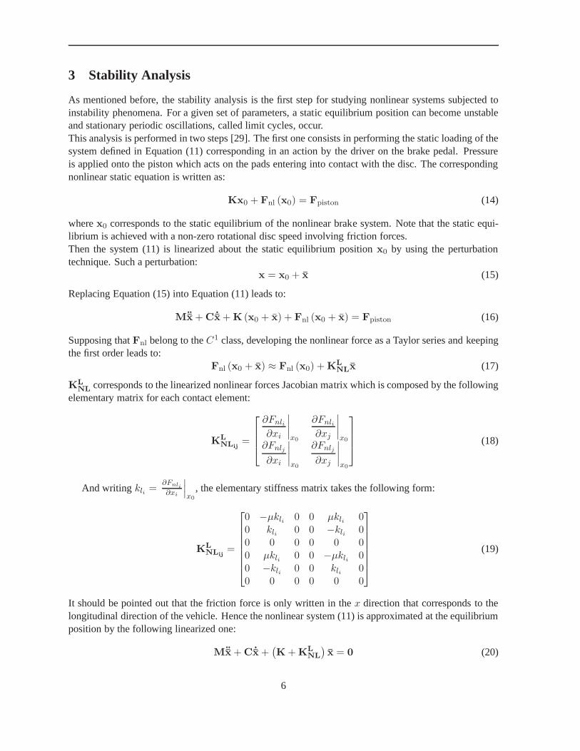
As mentioned before, the stability analysis is the first stepfor studying nonlinear systems subjected toinstability phenomena. For a given set of parameters, a static equilibrium position can become unstableand stationary periodic oscillations, called limit cycles, occur.This analysis is performed in two steps [29]. The first one consists in performing the static loading of thesystem defined in Equation (11) corresponding in an action bythe driver on the brake pedal. Pressureis applied onto the piston which acts on the pads entering into contact with the disc. The correspondingnonlinear static equation is written as:
Kx0 + Fnl (x0) = Fpiston (14)
wherex0 corresponds to the static equilibrium of the nonlinear brake system. Note that the static equi-librium is achieved with a non-zero rotational disc speed involving friction forces.Then the system (11) is linearized about the static equilibrium positionx0 by using the perturbationtechnique. Such a perturbation:
x = x0 + x (15)
Replacing Equation (15) into Equation (11) leads to:
M¨x+C ˙x+K (x0 + x) + Fnl (x0 + x) = Fpiston (16)
Supposing thatFnl belong to theC1 class, developing the nonlinear force as a Taylor series andkeepingthe first order leads to:
Fnl (x0 + x) ≈ Fnl (x0) +KL
NLx (17)
KL
NLcorresponds to the linearized nonlinear forces Jacobian matrix which is composed by the following
elementary matrix for each contact element:
KL
NLij=
∂Fnli
∂xi
∣
∣
∣
∣
x0
∂Fnli
∂xj
∣
∣
∣
∣
x0
∂Fnlj
∂xi
∣
∣
∣
∣
x0
∂Fnlj
∂xj
∣
∣
∣
∣
x0
(18)
And writing kli =∂Fnli
∂xi
∣
∣
∣
x0
, the elementary stiffness matrix takes the following form:
KL
NLij=
0 −µkli 0 0 µkli 00 kli 0 0 −kli 00 0 0 0 0 00 µkli 0 0 −µkli 00 −kli 0 0 kli 00 0 0 0 0 0
(19)
It should be pointed out that the friction force is only written in thex direction that corresponds to thelongitudinal direction of the vehicle. Hence the nonlinearsystem (11) is approximated at the equilibriumposition by the following linearized one:
M¨x+C ˙x+(
K+KL
NL
)
x = 0 (20)
6

a b
0.7 0.8 0.9 1 1.1 1.2 1.3 1.4 1.5 1.6−0.8
−0.6
−0.4
−0.2
0
0.2
0.4
0.6
0.8
Normalized Friction Coefficient
Nor
mal
ized
Rea
l Par
t
0.7 0.8 0.9 1 1.1 1.2 1.3 1.4 1.5 1.60.9985
0.999
0.9995
1
1.0005
1.001
1.0015
Normalized Friction Coefficient
Nor
mal
ized
Fre
quen
cy
Figure 2: Stability analysis (a) Evolution of the real partsof the stable and unstable modes (b) Coales-cence of the two corresponding eigenvalues
The previous model (20) is then written in the following state-space and complex eigenvalues are de-rived :
A =
[
0 I
−M−1(
K+KL
NL
)
−M−1C
]
(21)
Since the stiffness matrix (19) is asymmetrical due to the contribution of friction forces, the computedeigenvalues are complex and are written as:
λ = a+ iω (22)
wherea is the real part of the eigenvalue that corresponds to the growth rate of the amplitude andωis the imaginary part of the eigenvalue that corresponds to the pulsation of the mode. A negative realpart indicates that the corresponding mode is stable. In other words, a perturbation about the staticequilibrium sliding state will not modify the equilibrium position of the system. A positive real partequivalent to a negative damping leads to an unstable mode. Thus modifying one of the parameterswill induce growing oscillations about the static equilibrium position of the system until the dynamicalsteady-state is reached. Figure 2 shows evolutions of normalized real parts and normalized frequencies ofthe associated eigenvalue versusµ, which is normalized with respect to the Hopf bifurcation point µ0. Asseen in Figure 2(a), the real parts curves split into two branches near the Hopf bifurcation pointµ0. Onegoes towards the positive real part half-space and become positive whereas the other branch decreasesand remains in the negative real part half-space. Figure 2(b) shows the typical lock-in phenomenonbetween both modes of the system withµ increasing. It can be seen that coalescence between the twomodes is perfect since they are equally damped. The effects of equally and non-equally damped modeswill be illustrated in the last part of this paper. It is then possible to define stable areas versus unstableareas of the linearized system for a given set of parameters.In the following, the paper is devoted tononlinear dynamic computation.
7

4 Non-linear dynamic and self-excited limit cycles
The classical approach of nonlinear analysis consists in using temporal integration schemes to computenonlinear dynamic solutions. However, it can be observed that this kind of method is costly in terms ofcomputation time and resources for large finite element models.Enhanced nonlinear methods have to be employed to save time.Extensive reviews on this topic havebeen given in [30]. In the following part of the paper, an original adaptation of the harmonic balancemethod for self-excited nonlinear systems will be introduced and discussed.
4.1 The Constrained Harmonic Balance Method
In this section, we propose to introduce an extension of the harmonic balance method, called the Con-strained Harmonic Balance Method (CHBM), for approximating stationary nonlinear responses of self-excited systems subjected to flutter instabilities. Traditional harmonic balance methods are well-knownnumerical methods that have been commonly used to solve nonlinear problems in engineering [30].However, they do not permit obtaining the stationary nonlinear vibrational responses of self-excited sys-tems due to the fact that the static nonlinear solution corresponds to the trivial solution of the problem.In this section, the classical harmonic balance method witha condensation procedure on the nonlineardofs is presented first. Then the additional constraining condition allowing the determination of the limitcycle amplitudes and an optimized initial condition process are presented and discussed.
4.1.1 The Harmonic Balance Method with a condensation procedure
Considering harmonic balance methods, a nonlinear solution is assumed to be a truncated Fourier seriesand the exact nonlinear periodic solutionX (t) is replaced as:
Xapp (t) =
Nh∑
k=0
UC
k cos (kωt) +
Nh∑
k=1
US
k sin (kωt) (23)
whereUC
k andUS
k are vectors of Fourier coefficients andω defines the final pulsation of the nonlinearlimit cycles. It can be seen thatω is an unknown parameter in this study since we are in the presence of aself-excited system and the frequency of the stability analysis differs slightly from that of the nonlinearsteady-state solution. Thus it cannot be used as a fixed parameter. Nh is the number of the harmoniccoefficients retained for the approximated nonlinear stationary solution. Velocities and accelerations areobtained by derivation of Equation (23) with respect to the time. The advantage of harmonic balancemethod is that it allows keeping only the first terms of Equation (23) where, generally, a preponderantenergy part of the signal is concentrated.Replacing the approximated solutionXapp (t) into Equation (11) leads to
RNh(t) =
Nh∑
k=0
[(
K− (kω)2M)
UC
k + (kωC)US
k
]
cos (kωt)+
Nh∑
k=1
[(
K− (kω)2M)
US
k − (kωC)UC
k
]
sin (kωt) + Fnl
(
UC,Sk
)
− Fpiston
(24)
Projecting the residue on sine and cosine orthonormal bases, and writing the multi-harmonics vectorUsuch that:
8

U =[
UC0
TUC
1
TUS
1
T· · · UC
Nh
TUS
Nh
T]T
(25)
leads to the following approximated equation:
ΛU+ Fnl
(
U)
= Fout (26)
with
Λ =
K 0 0 0 0 0
0 Λh,1 0 0 0 0
0 0. . . 0 0 0
0 0 0 Λh,k 0 0
0 0 0 0. . . 0
0 0 0 0 0 Λh,Nh
(27)
and
Λh,k =
[
−(kω)2M+K kωC−kωC −(kω)2M+K
]
for k = 1 : Nh (28)
Λh,k is the dynamical stiffness matrix associated with thekth harmonic andFout are the external forces.Equation (25) gathers the Fourier coefficients that have to be balanced to obtain the periodic solution ofthe nonlinear system. Non-linear force Fourier coefficients depend onU and their determination can befastidious analytically because of the size of the system and the number of harmonics. The AlternateFrequency Time Domain Method proposed by Cameron and Griffin[22] permits omitting this issue asoutlined below:
UFFT−1
−→ X (t) −→ Fnl (X(t))FFT−→ Fnl
(
U)
(29)
When a nonlinear system has a significant number of dofs but only a few of then are related to nonlinearcomponents, it is possible to reduce system (26) on the nonlinear dofs without loss of accuracy [31,32].Linear and nonlinear nodes are separated (i.e. the new vector is such that the nonlinear dofs are stored atthe vector’s end). Equation (26) may be rewritten in the following form
[
Λln,ln Λln,nl
Λnl,ln Λnl,nl
]{
Uln
Unl
}
+
{
0
Fnl
}
=
{
Fout,ln
Fout,nl
}
(30)
whereUln andUnl define the linear dofs and nonlinear dofs, respectively.Fout,ln andFout,nl are the as-sociated linear and nonlinear external forces. In the current model, only external linear force is available,i.e. the piston force.The purpose of the condensation aims at solving the algebraic nonlinear system of equations only fornonlinear dofs, leaving the other linear ones to be determined later by a linear transformation. Hencerewriting (30) on nonlinear dofs leads to:
ΛeqUnl + Fnl (Unl) = Feq (31)
withΛeq = Λnl,nl −Λnl,ln (Λln,ln)
−1Λln,nl (32)
andFeq = Fout,nl −Λnl,ln (Λln,ln)
−1Fout,ln (33)
9

Thus system (31) has the size of the number of nonlinear dofs and is lighter than (30). Equation (31) isrewritten in the following form to be solved:
f(
Unl
)
= ΛeqUnl + Fnl
(
Unl
)
− Feq (34)
When optimization is finished andUnl is known, linear displacements are obtained with:
Uln = Λ−1ln,ln
(
Fout,ln −Λln,nlUnl
)
(35)
4.1.2 The additional constraining condition
Equation (34) is a cost function that has a minimum whenUnl is a solution of the system and can besolved by nonlinear least-square algorithms such as those of the Gauss-Newton and Leveberg-Marquardtmethods. As stated before, the uniqueness of the solution islost for systems at the Hopf bifurcationpoint [11]: the exact and trivial solution of Equation (34) corresponds to the static equilibrium pointwhich is unstable. If the classical Harmonic balance Methodis used, the only solution that will be foundwill be this static solution due to the fact that the residue of Equation (34) will be equal to zero for thestatic equilibrium point. So, in order to reject this trivial static solution and obtain the stationary nonlineardynamical oscillations that correspond to the limit cycle amplitudes, it is necessary to add a constraintto the Harmonic Balance Method to reach only the minimum of Equation (34) which corresponds to thestationary nonlinear periodic motion. The constraining condition will be outlined in this paragraph.By considering the nonlinear autonomous system (11) and writing it in the state space gives:
Y = AY + FP + FNL (Y) (36)
with
Y =
{
X
X
}
, FP =
{
0
M−1Fpiston
}
, FNL =
{
0
−M−1Fnl
}
(37)
and
A =
[
0 I
−M−1K −M−1C
]
(38)
A nonlinear periodic solutionYe(t) of Equation (36) is such that a realT exists so that:
Ye(t+ T ) = Ye(t) andYe(t+ T ) 6= Ye(t) for 0 < T < T (39)
T is the period of the solution. It may be noted thatT is an unknown parameter due to the absence offorced excitations and the difference between the stability frequency analysis and that of the nonlinearsystem.By disturbing a solutionYe(t) with a perturbationǫ(t) we obtain:
Y(t) = Ye(t) + ǫ(t) (40)
And by substituting Equation (40) in Equation (39), we obtain:
Ye + ǫ = A (Ye + ǫ) + FP + FNL (Ye + ǫ) (41)
By supposing thatFNL is C1 class, its development in the Taylor series atYe at the first order gives
Ye + ǫ ≈ A (Ye + ǫ) + FP + FNL (Ye) + JNLǫ (42)
10

with JNL the Jacobian matrix of the first derivatives of the nonlinearforcesFNL respect to the periodicsolutionYe(t).SinceYe(t) is the solution of Equation (36), Equation (42) is under the form
ǫ ≈ Aǫ+ JNLǫ = Jǫ (43)
withJ = A+ JNL (44)
J is the Jacobian matrix of the nonlinear system (36) and depends on the dynamical solutionYe(t).Thereby the eigenvalues ofJ define the evolution of the limit cycles amplitudes of the nonlinear system.If one or more eigenvalues are positive, the approximated nonlinear solution of the system is increasingand is governed by the unstable modes. If all the eigenvaluesare negative, the nonlinear solution isdecreasing (i.e. we are still in transient motion). If one eigenvalue is equal to zero whereas all the othersare negative, the nonlinear approximated solution defines the stationary motion of the nonlinear systemsubjected to flutter instability.
The replacement of the nonlinear contributionsFNL by a linear approximationJNL is done to mini-mize the differenceζ
ζ = FNL (Ye(t))− JNLYe(t) (45)
This kind of transformation refers to the equivalent linearization concept proposed by Iwan [33]. Finally,ζ can be minimized by using a least square method.It may be noted thatJNL is the Jacobian matrix of the periodic nonlinear forces and does not depend ontime. The eigenvalues ofJ are clearly related to the evolution of the nonlinear periodic solutionYe(t).Indeed, the real part of the corresponding unstable mode becomes equal to zero while the other real partsare negative when the computed solution has reached dynamical steady-state.
Hence the unstable real part is used as an extra equation for the root finding algorithm. In such acase, it will converge towards the steady-state solution where the dynamical equation and the real partare minimized.In conclusion, the final set of equations that has to be minimized is given by the two following functions
f1
(
Unl, ω)
andf2(
Unl, ω)
f1
(
Unl, ω)
= Λeq (ω) Unl + Fnl
(
Unl, ω)
− Feq < ǫ1 (46)
f2
(
Unl, ω)
= |Re (λ) | < ǫ2 (47)
whereλ defines the eigenvalue ofJ that has the maximum real part.ǫ1 and ǫ2 are chosen residualcoefficients.The complete procedure and description of the Constrained Harmonic Balance Method is given in Figure3.
4.1.3 The optimized additional initial conditions
As explained previously, the unknown parameters that have to be determined are the Fourier coefficientsUnl and the frequencyω of the stationary periodic signal.Firstly, when employing the static equilibrium position asthe initial condition, computation can be verydifficult and expensive. Hence they are too far from the final stationary nonlinear dynamical solution and
11

so another initial estimation must be determined to save time and improve the computation procedure.In this part of the paper, optimized additional initial conditions based on the complex nonlinear modalanalysis [34] are introduced and discussed.As explained previously by Sinou et al. [34], starting from the hypothesis that the nonlinear unstablemode drives the dynamical solution, the evolution of the approximated solution curve, defined by con-sidering only the contribution of the unstable mode, is given by:
Y0(t, p, λ) = p(
Ψeλt + Ψeλt)
(48)
whereΨ defines the nonlinear unstable mode andΨ its conjugate.λ is the eigenvalue that correspondsto the unstable mode andp is an arbitrary chosen coefficient.The optimized additional initial conditions are defined as the decomposition into Fourier coefficients ofthe previous expression ofY0 (t, p, λ). In this case,Ψ is the eigenvector of the nonlinear unstable modethat has been obtained from the stability analysis. These optimized initial conditions work for quite awide range ofp and lead to the convergence of the harmonic balance method for the first calculation.Afterwards it is easy to compute solutions for given sets of parameters starting from previous results.Secondly, when using the harmonic balance method it is necessary to know the frequency of the periodicsignal since the dynamical matrices are frequency-dependent and thus convergence may be laborious oreven impossible if the chosen frequency is too approximative. The initial frequency value is selected tobe equal to the unstable mode frequency computed by stability analysis. Figure 3 displays the algorithmprocedure of the Constrained Harmonic Balance Method.
5 Results
In this part of the paper, the effectiveness of the Constrained Harmonic Balance Method will be illustratedfor the nonlinear brake system presented in Section 2.
5.1 Non-linear stationary solutions
Limit cycles are computed forµ = µ0 for cases with1, 2, 3 and10 harmonics. Results are comparedwith those obtained by applying temporal integration. The results shown in Figures 4 (a-b) correspondto a physical interface node where previous static reductions have been performed together with a modaldisplacement (c-d). First of all, the case with only one harmonic is discussed. Considering Figure 4,it clearly appears that the approximated solution obtainedwith one harmonic does not converge exactlywith the final temporal solution. However, this solution gives a initial approximation of the limit cycleamplitudes, indicating that the first harmonic is one of the most significant components for the completenonlinear solution. Hence estimations of the approximatednonlinear solutions computed with2 or 3harmonics are considered. The nonlinear limit cycles show agood fit with the temporal integrationresults in Figure 4. Moreover, the computed unknown frequency from the CHBM is very close to thatof the temporal integration since the difference is less than 0.03% for 1,2, 3 and10 harmonics. To makeunderstanding easier for the reader, the evolutions of the residue of the nonlinear equation are givenin Figure 7 for each case. Computational tests have been performed by assuming that the frequencyof the limit cycles is different from the frequency obtainedfrom the stability analysis. For the readercomprehension, neglecting changes in frequency of the self-excited nonlinear vibrations does not allowgood estimation of the limit cycle amplitudes even if the difference between the frequency obtained fromthe stability analysis and the fundamental frequency of thenon-linear oscillations appears to be very
12

Figure 3: Algorithm procedure
small.When looking at Figures 4 (c-d), it is obvious that more complex solutions are better estimated whenaugmenting the number of harmonics. Slight differences appear between2 and3 harmonics because thethird order becomes no more negligible and has to be taken into account for matching curves from thenumerical integration well. This is even true for higher nonlinearities which generally involve couplingbetween Fourier coefficients and thus higher order responses. All the limit cycles computed with10harmonics match numerical integration correctly. Table 1 summarizes the results and relative errors forthe three cases studied.Finally, Figure 5 shows the power spectrum ratios of the limit cycles computed atµ = µ0 for eachharmonic. Computation is done by summing power of each dof for a given harmonic:
Pj =1
2
Ndof∑
i=1
(
a2i,j + b2i,j)
(49)
13
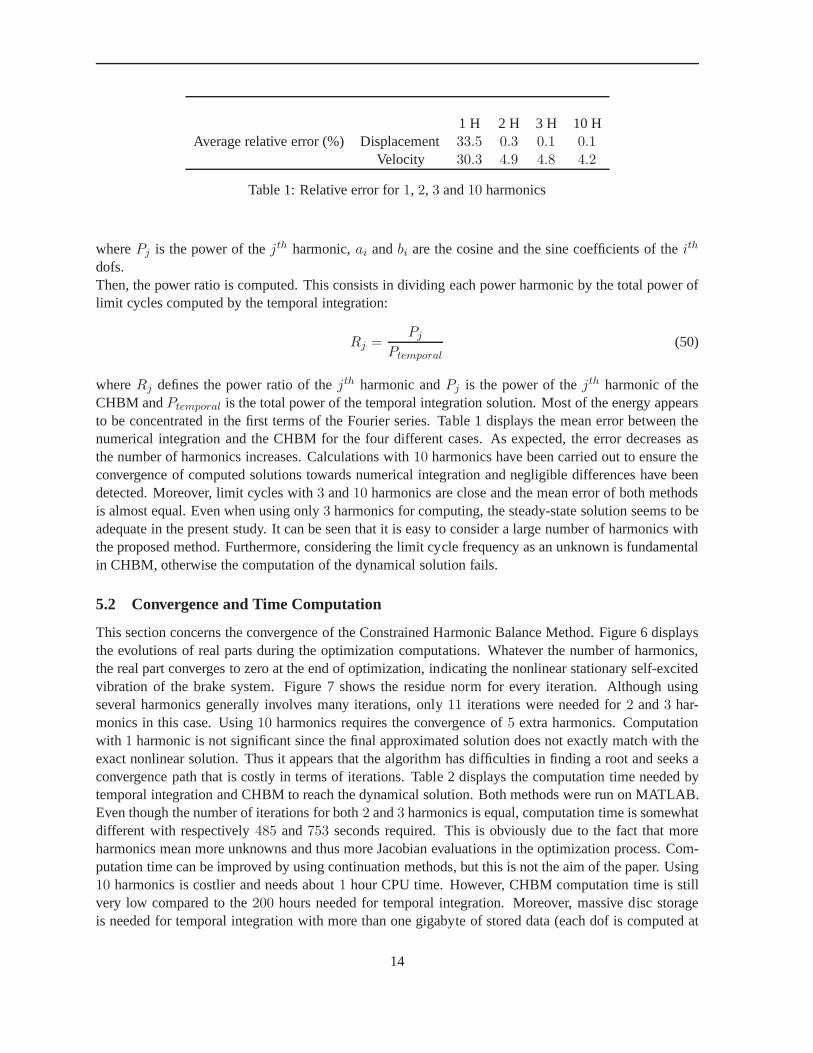
1 H 2 H 3 H 10 HAverage relative error (%) Displacement33.5 0.3 0.1 0.1
Velocity 30.3 4.9 4.8 4.2
Table 1: Relative error for1, 2, 3 and10 harmonics
wherePj is the power of thejth harmonic,ai andbi are the cosine and the sine coefficients of theith
dofs.Then, the power ratio is computed. This consists in dividingeach power harmonic by the total power oflimit cycles computed by the temporal integration:
Rj =Pj
Ptemporal(50)
whereRj defines the power ratio of thejth harmonic andPj is the power of thejth harmonic of theCHBM andPtemporal is the total power of the temporal integration solution. Most of the energy appearsto be concentrated in the first terms of the Fourier series. Table 1 displays the mean error between thenumerical integration and the CHBM for the four different cases. As expected, the error decreases asthe number of harmonics increases. Calculations with10 harmonics have been carried out to ensure theconvergence of computed solutions towards numerical integration and negligible differences have beendetected. Moreover, limit cycles with3 and10 harmonics are close and the mean error of both methodsis almost equal. Even when using only3 harmonics for computing, the steady-state solution seems to beadequate in the present study. It can be seen that it is easy toconsider a large number of harmonics withthe proposed method. Furthermore, considering the limit cycle frequency as an unknown is fundamentalin CHBM, otherwise the computation of the dynamical solution fails.
5.2 Convergence and Time Computation
This section concerns the convergence of the Constrained Harmonic Balance Method. Figure 6 displaysthe evolutions of real parts during the optimization computations. Whatever the number of harmonics,the real part converges to zero at the end of optimization, indicating the nonlinear stationary self-excitedvibration of the brake system. Figure 7 shows the residue norm for every iteration. Although usingseveral harmonics generally involves many iterations, only 11 iterations were needed for2 and3 har-monics in this case. Using10 harmonics requires the convergence of5 extra harmonics. Computationwith 1 harmonic is not significant since the final approximated solution does not exactly match with theexact nonlinear solution. Thus it appears that the algorithm has difficulties in finding a root and seeks aconvergence path that is costly in terms of iterations. Table 2 displays the computation time needed bytemporal integration and CHBM to reach the dynamical solution. Both methods were run on MATLAB.Even though the number of iterations for both2 and3 harmonics is equal, computation time is somewhatdifferent with respectively485 and753 seconds required. This is obviously due to the fact that moreharmonics mean more unknowns and thus more Jacobian evaluations in the optimization process. Com-putation time can be improved by using continuation methods, but this is not the aim of the paper. Using10 harmonics is costlier and needs about1 hour CPU time. However, CHBM computation time is stillvery low compared to the200 hours needed for temporal integration. Moreover, massive disc storageis needed for temporal integration with more than one gigabyte of stored data (each dof is computed at
14

a b
1.64 1.66 1.68 1.7 1.72 1.74 1.76
x 10−3
−0.6
−0.4
−0.2
0
0.2
0.4
0.6
Displacement (m)
Vel
ocity
(m
.s−1 )
1.7449 1.745 1.74511.74521.74531.74541.74551.74561.74571.7458
x 10−3
−0.08
−0.06
−0.04
−0.02
0
0.02
0.04
0.06
0.08
Displacement (m)
Vel
ocity
(m
.s−1 )
c d
−4 −3 −2 −1 0 1 2 3 4 5
x 10−8
−6
−4
−2
0
2
4
6x 10
−4
Displacement (m)
Vel
ocity
(m
.s−1 )
−3.5 −3 −2.5 −2 −1.5 −1
x 10−8
−1.5
−1
−0.5
0
0.5
1
1.5
2x 10
−4
Displacement (m)
Vel
ocity
(m
.s−1 )
Figure 4: Limit cycles using the classical temporal integration and the modified HBM atµ0; — temporalintegration, —1 harmonic, - -2 harmonics, -.-3 harmonics, ...10 harmonics; (b,d) zoom
each timet and stored on the disc) compared to a few kilobytes used by theFourier coefficients of theCHBM. In the following part of this paper3 harmonics will be used, regarding noticeably low relativeerrors both on displacement and on velocity. Moreover it offers a good compromise between accuracyand computation time. In conclusion, the proposed Constrained Harmonic Balance Method is well de-signed for a self-excited system because the results are accurate regarding the temporal approach and itis cheaper in terms of time consumption and disc storage.
6 Parametric studies : Interest of the CHBM
In this section of the paper, parametric studies will be undertaken for both the stability analysis and thelimit cycles amplitudes.
6.1 Friction coefficient
The friction coefficient is generally considered as one of the most important parameters in brake systems.Good brake performances often signify a high friction coefficient yielding a high sound pressure level.Limit cycles are computed forµ = µ0, µ = 1.2µ0, µ = 1.4µ0, µ = 1.6µ0 andµ = 2µ0 and displayed
15

1 2 3 4 5 6 7 8 9 1010
−8
10−7
10−6
10−5
10−4
10−3
10−2
10−1
100
Pow
er R
atio
Harmonic Order
Figure 5: Power ratio for the first10 harmonics
Methods Temporal Integration HBM1H HBM 2H HBM 3H HBM 10HIteration Numbers – 60 11 11 16Time Computation 200 hours 1550 seconds 485 seconds 753 seconds 3591 seconds
Disc Storage 1.4 Go 4 ko 6 ko 8 ko 9 ko
Table 2: Performance computation
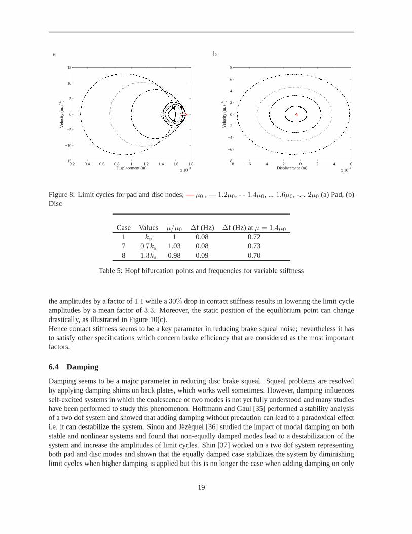
on Figure 8.In the rest of the study, the real parts as well as the frequencies computed and displayed in tables arenormalized in relation to those in the nominal model (i.e.P0, ks, µ0 andD1 = D2 = 1). To demonstratethe interest of considering the frequency as an unknown in the nonlinear method proposed in this paper,Table 3 gives the difference∆f between the initial frequency of the unstable mode that hasbeen obtainedvia the stability analysis for the nominal parameters and the final frequency of the self-excited vibrationthat has been obtained via the nonlinear method.Considering Figures 8, it clearly appears that increasing the friction coefficient involves the higher vi-bration amplitudes for both pad and disc. Moreover, evolutions of the equilibrium point are observed, asindicated in Figure 8(a).It can be seen that the Constrained Harmonic Balance Method allows determining the limit cycle ampli-tudes not only in the vicinity of the Hopf bifurcation point but also far from the Hopf bifurcation pointµ0. In Table 3, a difference between the frequency of the limit cycle amplitudes and the frequency of theunstable mode can be observed.
16

a b
0 10 20 30 40 50 60−5
0
5
10
15R
eal P
art
Iterations2 4 6 8 10 12 14 16
−0.5
0
0.5
1
1.5
2
2.5
Rea
l Par
t
Iterations
Figure 6: Evolution of the real part; —1 harmonic, - -2 harmonics, -.-3 harmonics, ...10 harmonics (a)all cases (b) zoom on2, 3 and10 harmonics
Case Values ∆f (Hz)1 µ0 -0.0442 1.2µ0 0.453 1.4µ0 0.714 1.6µ0 0.905 2µ0 1.2
Table 3: Hopf bifurcation points and frequencies for variable friction coefficient
6.2 Piston pressure
A variation in piston pressure has an effect on the pressure distribution at the disc/pad interface and thestability analysis of the brake system may be affected. Eigenvalues are computed for three differentpressures0.8P0, P0 and1.2P0 whereP0 is the operational piston pressure. The evolutions of the realparts and the coalescences of the unstable and stable modes are illustrated in Figures 9(a-b). Table 4gives the evolution of the Hopf bifurcation point. It appears that the pressure has an important effect ofthe stability. Basically, a higher piston pressure increases the degree of instability by moving the Hopfbifurcation point towards lower values without modifying the pattern shapes of the evolution of the realpart or frequency coalescences. However, the frequency coalescence point is affected by a change inpiston pressure, typically a high piston pressure results in a higher coupled frequency.Figures 9(c-d) illustrate the limit cycle amplitudes for the pad and the disc. To facilitate comprehension,the nonlinear vibrations are obtained at a fixed normalized friction coefficientµ = 1.05µ0. Hence padinterface deformation is equivalent for the three cases although the static positions are more affected fornodes at the pad/piston interface (see Figures 9(c)). This fact can be clearly explained by consideringthat higher piston pressure results in greater pad compression. The piston/pad interface is moved towardspad/disc interface. Disc deformation interface (Figure 9 (d)) is slightly impacted with an increase in
17

a b
0 10 20 30 40 50
100
102
104
Nor
m o
f Res
idue
Iterations2 4 6 8 10 12 14
10−2
100
102
104
Nor
m o
f Res
idue
Iterations
Figure 7: Evolution of residues during optimization; —1 harmonic, - -2 harmonics, -.-3 harmonics, ...10 harmonics (a) all cases (b) zoom on2, 3 and10 harmonics
Case Values µ/µ0 ∆f (Hz) ∆f (Hz) atµ = 1.4µ0
1 P0 1 0.14 0.725 0.8P0 1.04 0.15 0.726 1.2P0 0.96 0.13 0.72
Table 4: Hopf bifurcation points and frequencies for variable piston pressure
vibration amplitudes as the piston pressure increases.
6.3 Contact Stiffness
This part is devoted to the analysis of contact stiffness applied to the problem of brake squeal phe-nomenon. This parameter is very dependent on contact body stiffness and contact surface shapes. Sincethe disc is about a thousand times stiffer than the pad, contact stiffness usually depends on frictionalmaterials. Both analyses are performed for three contact stiffnesses corresponding to a variation of thepad friction material’ properties. For the sake of simplicity, ks is considered as a function of linearkl andnonlinearknl contact stiffness springs,ks = f(kl, knl). The evolution of the real parts and frequenciesof the stable and unstable modes are shown in Figures 10(a-b). Table 5 gives the evolution of the Hopfbifurcation point. As for the piston pressure case, an increase in the contact stiffness destabilizes thenonlinear system by decreasing the Hopf bifurcation point.Nevertheless, the patterns look alike andonly a translation is observed for varyingks. Frequency lock-in is changed and a higher contact stiffnessresults in augmenting the coalescence frequency. This is quite logical since high contact stiffness tendsto rigidify the whole system and thus increase the resonancefrequencies.When looking at limit cycles on Figure 10(c-d) which are computed forµ = 1.03µ0, it can be seenthat increasing the contact stiffness decreases the nonlinear vibrations. Nevertheless, amplitudes do notchange with the same ratio compared to the variable stiffness. A 30% increase in stiffness only changes
18
a b
0.2 0.4 0.6 0.8 1 1.2 1.4 1.6 1.8
x 10−3
−15
−10
−5
0
5
10
15
Displacement (m)
Vel
ocity
(m
.s−1 )
−8 −6 −4 −2 0 2 4 6
x 10−4
−8
−6
−4
−2
0
2
4
6
8
Displacement (m)
Vel
ocity
(m
.s−1 )
Figure 8: Limit cycles for pad and disc nodes;— µ0 , — 1.2µ0, - - 1.4µ0, ... 1.6µ0, -.-. 2µ0 (a) Pad, (b)Disc
Case Values µ/µ0 ∆f (Hz) ∆f (Hz) atµ = 1.4µ0
1 ks 1 0.08 0.727 0.7ks 1.03 0.08 0.738 1.3ks 0.98 0.09 0.70
Table 5: Hopf bifurcation points and frequencies for variable stiffness
the amplitudes by a factor of1.1 while a30% drop in contact stiffness results in lowering the limit cycleamplitudes by a mean factor of3.3. Moreover, the static position of the equilibrium point canchangedrastically, as illustrated in Figure 10(c).Hence contact stiffness seems to be a key parameter in reducing brake squeal noise; nevertheless it hasto satisfy other specifications which concern brake efficiency that are considered as the most importantfactors.
6.4 Damping
Damping seems to be a major parameter in reducing disc brake squeal. Squeal problems are resolvedby applying damping shims on back plates, which works well sometimes. However, damping influencesself-excited systems in which the coalescence of two modes is not yet fully understood and many studieshave been performed to study this phenomenon. Hoffmann and Gaul [35] performed a stability analysisof a two dof system and showed that adding damping without precaution can lead to a paradoxical effecti.e. it can destabilize the system. Sinou and Jezequel [36] studied the impact of modal damping on bothstable and nonlinear systems and found that non-equally damped modes lead to a destabilization of thesystem and increase the amplitudes of limit cycles. Shin [37] worked on a two dof system representingboth pad and disc modes and shown that the equally damped casestabilizes the system by diminishinglimit cycles when higher damping is applied but this is no longer the case when adding damping on only
19

a b
0.7 0.8 0.9 1 1.1 1.2 1.3 1.4 1.5 1.6−0.8
−0.6
−0.4
−0.2
0
0.2
0.4
0.6
0.8
Normalized Friction Coefficient
Nor
mal
ized
Rea
l Par
t
0.7 0.8 0.9 1 1.1 1.2 1.3 1.4 1.5 1.60.9985
0.999
0.9995
1
1.0005
1.001
1.0015
Normalized Friction Coefficient
Nor
mal
ized
Fre
quen
cy
c d
5 5.5 6 6.5 7 7.5 8
x 10−3
−4
−3
−2
−1
0
1
2
3
4
Displacement (m)
Vel
ocity
(m
.s−1 )
−8 −7 −6 −5 −4 −3 −2
x 10−5
−0.4
−0.3
−0.2
−0.1
0
0.1
0.2
0.3
Displacement (m)
Vel
ocity
(m
.s−1 )
Figure 9: Influence of piston pressure; —P0 , - - 0.8P0 , ... 1.2P0 (a) Evolution of real parts (b)Frequency coalescences; Limit cycles for (c) Pad, (d) Disc
one mode. While the amplitude of the more highly damped system decreases, the amplitude of the otherone increases. More recently, Fritz et al. [38,39] performed stability analyses on a complete finite elementmodel brake system. He confirmed that the ratio of the dampingof the two modes involved in squeal isan essential key for controlling the stability of systems. For equally damped modes, the stability curvesare lower and thus instability occurs for a higher friction coefficient. Nevertheless, in the case of largenon-equally damped modes a smoothing effect occurs and pushes the Hopf bifurcation point towardslower values, thus instability appears for a lower frictioncoefficient compared to the equally dampedcase.In the following, we investigate the effects of modal damping on stability and its impact on limit cycleamplitudes. Both the cases of equally and non-equally damped modes will be considered.
20
a b
0.7 0.8 0.9 1 1.1 1.2 1.3 1.4 1.5 1.6−0.8
−0.6
−0.4
−0.2
0
0.2
0.4
0.6
0.8
Normalized Friction Coefficient
Nor
mal
ized
Rea
l Par
t
0.7 0.8 0.9 1 1.1 1.2 1.3 1.4 1.5 1.60.9985
0.999
0.9995
1
1.0005
1.001
1.0015
Normalized Friction Coefficient
Nor
mal
ized
Fre
quen
cy
c d
1.5 1.55 1.6 1.65 1.7 1.75 1.8
x 10−3
−2
−1.5
−1
−0.5
0
0.5
1
1.5
2
Displacement (m)
Vel
ocity
(m
.s−1 )
−7 −6.5 −6 −5.5 −5 −4.5 −4 −3.5 −3 −2.5
x 10−5
−0.25
−0.2
−0.15
−0.1
−0.05
0
0.05
0.1
0.15
0.2
0.25
Displacement (m)
Vel
ocity
(m
.s−1 )
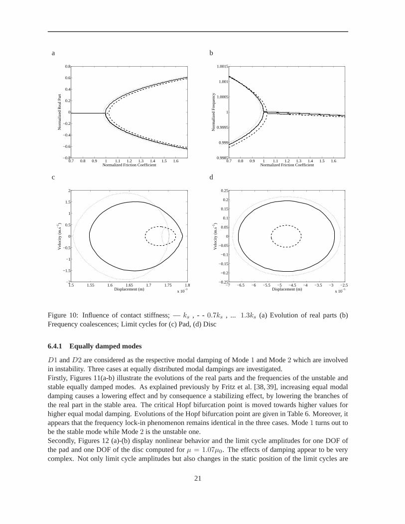
Figure 10: Influence of contact stiffness; —ks , - - 0.7ks , ... 1.3ks (a) Evolution of real parts (b)Frequency coalescences; Limit cycles for (c) Pad, (d) Disc
6.4.1 Equally damped modes
D1 andD2 are considered as the respective modal damping of Mode1 and Mode2 which are involvedin instability. Three cases at equally distributed modal dampings are investigated.Firstly, Figures 11(a-b) illustrate the evolutions of the real parts and the frequencies of the unstable andstable equally damped modes. As explained previously by Fritz et al. [38, 39], increasing equal modaldamping causes a lowering effect and by consequence a stabilizing effect, by lowering the branches ofthe real part in the stable area. The critical Hopf bifurcation point is moved towards higher values forhigher equal modal damping. Evolutions of the Hopf bifurcation point are given in Table 6. Moreover, itappears that the frequency lock-in phenomenon remains identical in the three cases. Mode1 turns out tobe the stable mode while Mode2 is the unstable one.Secondly, Figures 12 (a)-(b) display nonlinear behavior and the limit cycle amplitudes for one DOF ofthe pad and one DOF of the disc computed forµ = 1.07µ0. The effects of damping appear to be verycomplex. Not only limit cycle amplitudes but also changes inthe static position of the limit cycles are
21

Case D1 D2 D1/D2 µc/µH ∆f (Hz) ∆f (Hz) atµ = 1.4µ0
1 1 1 1 1 0.21 0.722 5 5 1 1.01 0.18 0.703 10 10 1 1.07 0.10 0.634 1 2 0.5 0.97 0.68 1.285 1 5 0.2 0.84 1.64 1.986 2 1 2 0.96 -0.50 0.247 5 1 5 0.84 -0.87 -0.18
Table 6: Hopf bifurcation points and frequencies for damping parameters
observed, as indicated in Figure 12(a). Surprisingly, the highly damped case does not necessarily inducelow vibration amplitudes. Although the vibration amplitudes of the pad are slightly higher for the lowerdamped case, the highest dynamical response of the disc is found for the highest damped case, with anamplitude ratio of almost4 in relation to the lowest damped case.Figures 12 (c)-(d) show limit cycles computed by increasingthe friction coefficient (µ = 1.4µ0 in thecurrent case). As explained previously in section 6.1, a higher friction coefficient involves higher limitcycle amplitudes. It can be seen that the effects of equally damped modes cannot be neglected and thatthe combined effect of the friction coefficient and damping is not trivial. For example, it appears thatthe influence of damping is weaker forµ = 1.4µ0 compared to the case in the vicinity of the Hopfbifurcation point atµ = 1.07µ0. For the disc, the amplitude is still highest for the larger damped case,but the amplitude ratio in relation to the lowest damped caseis less significant, with a value of1.3.Moreover, it can be noted that the nonlinear amplitudes of the limit cycles do not follow proportionallythe growth rate of the positive real part and the commonly held belief that the added damping wouldresult in lower vibrations is not necessarily true.
6.5 Non-equally damped modes
Now we investigate the influence of non-equally damped modesfor two cases that areD1/D2 = 0.5andD1/D2 = 0.2. Figures 11(c-d) illustrate the associated evolutions of the real parts and frequenciesof the unstable and stable equally damped modes. The reference remains the equally damped case whereD1/D2 = 1. It should be noted that the damping of unstable Mode2 turns out to be higher.The lowering effect due to high damping remains but its stabilizing effect is counterbalanced by the well-known smoothing effect occurring in the vicinity of the Hopfbifurcation point (see Figure 11(c)), asmentioned by [35–39]. The real part branches of non-equallydamped modes split with a smoother slopeand become positive at a lower friction coefficient than the real part branch of the equally damped mode.This effect is stronger for higher asymmetrical modal damping cases, for example whenD1/D2 = 0.2.
Figure 13 (a-b) illustrates the nonlinear limit cycles thatare computed atµ = µ0. The largest limitcycle amplitudes appear for the lowest damping ratio,D1/D2 = 0.2 although the unstable mode is themore highly damped one. More complex behavior is found for pad deformation whenD1/D2 = 0.2.With a higher friction coefficient, the real part curves cross each other at aroundµ = 1.03µ0 and caseD1/D2 = 1 has the larger positive real part, contrary to theD1/D2 = 0.2 case which becomes themost stable beyondµ = 1.03µ0. Figure 13 (c-d) presents the limit cycles of both the nodes consideredpreviously, computed atµ = 1.4µ0.
22

a b
0.7 0.8 0.9 1 1.1 1.2 1.3 1.4 1.5 1.6−0.8
−0.6
−0.4
−0.2
0
0.2
0.4
0.6
0.8
Normalized Friction Coefficient
Nor
mal
ized
Rea
l Par
t
0.7 0.8 0.9 1 1.1 1.2 1.3 1.4 1.5 1.60.9985
0.999
0.9995
1
1.0005
1.001
1.0015
Normalized Friction Coefficient
Nor
mal
ized
Fre
quen
cy
c d
0.7 0.8 0.9 1 1.1 1.2 1.3 1.4 1.5 1.6−0.8
−0.6
−0.4
−0.2
0
0.2
0.4
0.6
0.8
Normalized Friction Coefficient
Nor
mal
ized
Rea
l Par
t
0.7 0.8 0.9 1 1.1 1.2 1.3 1.4 1.5 1.60.9985
0.999
0.9995
1
1.0005
1.001
1.0015
Normalized Friction Coefficient
Nor
mal
ized
Fre
quen
cy
Figure 11: Evolution of real parts and frequency coalescences (a-b) equally damped: —1st case, - -2nd
case, ...3rd case (c-d) non-equally damped: —1st case, - -6th case, ...7th case
Large pad amplitudes are obtained for low damping ratios andare considered as the most stable casesatµ = 1.4µ0 by the stability analysis. Nevertheless, the highest amplitudes for the disc are derived fromthe most unstable case, which is the equally damped one. It can be clearly observed that it is not possibleto establish a link between the values of the real parts and corresponding vibrating states since they canbe higher or lower depending on the different effects of the physical parameters on both stability andnonlinear behavior. Moreover, it is noted that the static equilibrium point changes with the variation ofnon-equally damped modes, as indicated in Figure 13 (a).
To further investigate the influence of modal damping, we propose to invert damping ratiosD1/D2 =2, D1/D2 = 5 and perform a stability analysis and determine the nonlinear limit cycles. It should beborne in mind henceforth that stable Mode1 is the more highly damped one, whereas the damping ofunstable Mode2 is decreased. The evolutions of the real parts and frequencies of the stable and unstablemodes are similar to the previous case thus the conclusions on stability are identical.Figure 14 (a-b) and (c-d) illustrates the nonlinear limit cycles forµ = 1.07µ0 andµ = 1.4µ0, respec-
23
a b
1.5 1.55 1.6 1.65 1.7 1.75 1.8
x 10−3
−2.5
−2
−1.5
−1
−0.5
0
0.5
1
1.5
2
2.5
Displacement (m)
Vel
ocity
(m
.s−1 )
−2.5 −2 −1.5 −1 −0.5 0 0.5 1 1.5
x 10−4
−2
−1.5
−1
−0.5
0
0.5
1
1.5
2
Displacement (m)
Vel
ocity
(m
.s−1 )
c d
0.8 1 1.2 1.4 1.6 1.8
x 10−3
−8
−6
−4
−2
0
2
4
6
8
Displacement (m)
Vel
ocity
(m
.s−1 )
−5 0 5
x 10−4
−5
−4
−3
−2
−1
0
1
2
3
4
5
Displacement (m)
Vel
ocity
(m
.s−1 )
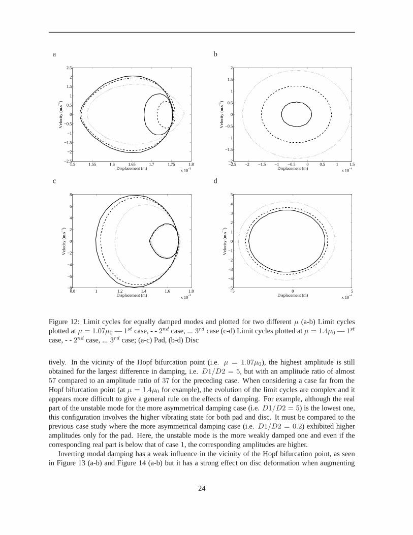
Figure 12: Limit cycles for equally damped modes and plottedfor two differentµ (a-b) Limit cyclesplotted atµ = 1.07µ0 — 1st case, - -2nd case, ...3rd case (c-d) Limit cycles plotted atµ = 1.4µ0 — 1st
case, - -2nd case, ...3rd case; (a-c) Pad, (b-d) Disc
tively. In the vicinity of the Hopf bifurcation point (i.e.µ = 1.07µ0), the highest amplitude is stillobtained for the largest difference in damping, i.e.D1/D2 = 5, but with an amplitude ratio of almost57 compared to an amplitude ratio of37 for the preceding case. When considering a case far from theHopf bifurcation point (atµ = 1.4µ0 for example), the evolution of the limit cycles are complex and itappears more difficult to give a general rule on the effects ofdamping. For example, although the realpart of the unstable mode for the more asymmetrical damping case (i.e.D1/D2 = 5) is the lowest one,this configuration involves the higher vibrating state for both pad and disc. It must be compared to theprevious case study where the more asymmetrical damping case (i.e. D1/D2 = 0.2) exhibited higheramplitudes only for the pad. Here, the unstable mode is the more weakly damped one and even if thecorresponding real part is below that of case1, the corresponding amplitudes are higher.
Inverting modal damping has a weak influence in the vicinity of the Hopf bifurcation point, as seenin Figure 13 (a-b) and Figure 14 (a-b) but it has a strong effect on disc deformation when augmenting
24

a b
1.45 1.5 1.55 1.6 1.65 1.7 1.75 1.8 1.85
x 10−3
−4
−3
−2
−1
0
1
2
3
4
Displacement (m)
Vel
ocity
(m
.s−1 )
−4 −3 −2 −1 0 1 2 3 4
x 10−4
−4
−3
−2
−1
0
1
2
3
4
Displacement (m)
Vel
ocity
(m
.s−1 )
c d
0.6 0.8 1 1.2 1.4 1.6 1.8
x 10−3
−15
−10
−5
0
5
10
15
Displacement (m)
Vel
ocity
(m
.s−1 )
−4 −3 −2 −1 0 1 2 3 4
x 10−4
−4
−3
−2
−1
0
1
2
3
4
Displacement (m)
Vel
ocity
(m
.s−1 )
Figure 13: Limit cycles for non-equally damped modes and plotted for two differentµ (a-b) Limit cyclesplotted atµ = µ0 — 1st case, - -4th case, ...5th case (c-d) Limit cycles plotted atµ = 1.4µ0 — 1st
case, - -4th case, ...5th case; (a-c) Pad, (b-d) Disc
the friction coefficient. When the unstable mode is the more strongly damped one, the limit cycles aresmaller than the equally damped case by a factor of 2 (Figure 13 (d)), but the conclusions are totallydifferent when inverting the damping ratio: The corresponding limit cycles are about 3 times larger thanfor the equally damped case (Figure 14 (d)) .
This example shows that inverting modal damping distribution has considerable effects not only onthe stability of the system but also on the nonlinear amplitudes of the limit cycles. For example, caseD1/D2 = 0.2 displays the smallest disc oscillations while caseD1/D2 = 5 has the largest disc os-cillations and the conclusions for finding the best model aretotally different. Considering the previousresults, it appears that structural damping is a key factor when dealing with nonlinear autonomous sys-tems, but nevertheless it is a complex phenomenon and it has to be considered with care to ensure goodsilent brake system design. Not only the quantity but also the distribution of damping have to be takeninto account thoroughly to avoid unexpected results.
25

a b
1.45 1.5 1.55 1.6 1.65 1.7 1.75 1.8 1.85
x 10−3
−4
−3
−2
−1
0
1
2
3
4
Displacement (m)
Vel
ocity
(m
.s−1 )
−6 −4 −2 0 2 4 6
x 10−4
−6
−4
−2
0
2
4
6
Displacement (m)
Vel
ocity
(m
.s−1 )
c d
0.6 0.8 1 1.2 1.4 1.6 1.8
x 10−3
−15
−10
−5
0
5
10
15
Displacement (m)
Vel
ocity
(m
.s−1 )
−1.5 −1 −0.5 0 0.5 1
x 10−3
−15
−10
−5
0
5
10
15
Displacement (m)
Vel
ocity
(m
.s−1 )
Figure 14: Limit cycles for non-equally damped modes and plotted for two differentµ (a-b)Limit cyclesplotted atµ = µ0 — 1st case, - -6th case, ...7th case (c-d) Limit cycles plotted atµ = 1.4µ0; — 1st
case, - -6th case, ...7th case; (a-c) Pad (b-d) Disc
7 Conclusion
In this paper proposed a novel nonlinear method called the Constrained Harmonic Balance Method. Thisoriginal approach allows the determination of the stationary nonlinear periodic solution of a nonlinearmechanical system subject to flutter instability, by the addition of an extra-constraint in the classical Har-monic Balance Method. This additional constraint allows eliminating the static equilibrium point (i.e.the trivial static solution of the nonlinear problem that would be obtained by applying the classical Har-monic Balance Method)) and gives only the stationary nonlinear oscillations. Moreover, the frequency isadded as an unknown since the frequency of a self-excited system is not knowna priori and may changefor varying parameters. Also, the dynamical solution cannot be computed if only using the frequencyresulting from the stability analysis. An application to disc brake squeal was performed to illustrate theeffectiveness of the nonlinear method.
26

Numerical results correlated well with a classical time domain algorithm in terms of both amplitude andfrequency. The results of the CHBM is highly dependent on thenumber of harmonics. A power ratiocomputation shows that the major part of the energy is concentrated in the first harmonic, but retainingonly the latter does not lead to the steady-state solution. In order to adapt to the complex behaviors of thesolutions, more harmonics are required in the Fourier series. The computation time of the new methodis very short compared to that of a classical temporal integration algorithm and thus is well designed forintensive computation in the case of parameter-dependent systems.The effectiveness of this method’s application to a disc brake system is emphasized in the last part of thepaper, which describes the parametric studies performed. Fast limit cycle computations were achievedfor a large number of operational parameters and conclusions were obtained. The complementarity be-tween the stability analysis and the complex nonlinear vibrational behavior appears to be essential forcarrying out a complete design study of a brake system. Moreover, it was shown that not only the frictioncoefficient, but also piston pressure, nonlinear stiffnessand structural damping are important factors totake into account to avoid poor design.
Acknowledge
Jean-Jacques Sinou gratefully acknowledges the financial support of the french National Research Agencythrough the program Young researcher ANR-07-JCJC-0059-01-CSD 2.
References
[1] Kinkaid, N., O’Reilly, O., and Papadopoulos, P., 2003. “Automotive disc brake squeal”.Journal ofSound and Vibration,267, pp. 105–166.
[2] North, M., 1972. Disc brake squeal, a theoretical model.Tech. rep., Motor Industry ResearchAssociation M.I.R.A.
[3] Ouyang, H., Mottershead, J., Cartmell, M., and Friswell, M., 1998. “Friction-induced parametricresonances in discs: effect of a negative friction-velocity relationship”. Journal of Sound andVibration,209(2), pp. 251–264.
[4] Ouyang, H., Mottershead, J., Cartmell, M., and Brookfield, D., 1999. “Friction-induced vibrationof an elastic slider on a vibrating disc”.International Journal of Mechanical Sciences,41, pp. 325–336.
[5] Spurr, R. T., 1961-1962. “A theory of brake squeal”.Proceedings of the Institution of MechanicalEngineers,No. 1, pp. 33–40.
[6] Jarvis, R., and Mills, B., 1963-1964. “Vibration induced by dry friction”. Proc. IMechE,178, No.32, pp. 847–866.
[7] Millner, N., 1978. “Analysis of disc brake squeal”. In SAE Paper, Vol. 780332.
[8] Oden, J., and Martins, J., 2003. “Model and computational methods for dynamic friction phenom-ena”. Computer Methods in Applied Mechanics and Engineering,52, pp. 527–634.
27

[9] Liles, G., 1989. “Analysis of disc brake squeal using finite element methods”. In SAE Paper,Vol. 891150.
[10] Ouyang, H., Mottershead, J., Brookfield, D., James, S.,and Cartmell, M., 2000. “Methodologyfor the determination of dynamic instabilities in a car discbrake”. International Journal of VehicleDesign,23(3), pp. 241–262.
[11] Moirot, F., 1998. “Etude de la stabilite d’un equilibre en presence de frottement de coulomb,application au crissement des freins a disque”. PhD thesis, Ecole Polytechnique.
[12] Nack, W., 2000. “Brake squeal analysis by finite elements”. International Journal of VehicleDesign,23(3,4), pp. 263–275.
[13] Kung, S., Dunlap, K. B., and Ballinger, R., 2000. “Complex eigenvalues analysis for reducing lowfrequency brake squeal”. In SAE Paper, Vol. 0444.
[14] Lorang, X., Foy-Margiocchi, F., Nguyen, Q., and Gautier, P., 2006. “Tgv disc brake squeal”.Journal of Sound and Vibration,293, pp. 735–746.
[15] Ouyang, H., Nack, W., Yuan, Y., and Chen, F., 2005. “Numerical analysis of automotive disc brakesqueal : a review”.International Journal of Vehicle Noise and Vibration,1(3/4).
[16] Massi, F., Baillet, L., Giannini, O., and Sestieri, A.,2007. “Linear and non-linear numerical ap-proaches”.Mechanical Systems and Signal Processing,21, pp. 2374–2393.
[17] Nagy, L., Cheng, J., and Hu, Y., 1994. “A new method development to predict squeal occurrence”.In SAE Paper, Vol. 942258.
[18] M.L., Dune, L., and Herting, D., 1997. “Nonlinear dynamics of brake squeal”.Finite Elements inAnalysis and Design,28, pp. 69–82.
[19] Mahajan, S., Hu, Y., and Zhang, K., 1999. “Vehicle disc brake squeal simulation and experiences”.In SAE Paper, Vol. 1738.
[20] Hu, Y., Mahajan, S., and Zhang, K., 1999. “Squeal doe using non-linear transient analysis”. InSAE Paper, Vol. 1737.
[21] AbuBakar, A., and Ouyang, H., 2006. “Complex eigenvalue analysis and dynamic transient anal-ysis in predicting disc brake squeal”.International Journal of Vehicle Noise and Vibration,2(2),pp. 143–155.
[22] Cameron, T., and Griffin, J., 1989. “An alternating frequency/time domain method for calculat-ing the steady-state response of nonlinear dynamic systems”. Journal of Applied Mechanics,56,pp. 149–154.
[23] Pierre, C., Ferri, A., and Dowell, E., 1985. “Multi-harmonic analysis of dry friction damped systemsusing an incremental harmonic balance method”.Journal of Applied Mechanics,52, pp. 958–964.
[24] Cheung, Y., Chen, S., and Lau, S., 1990. “Application ofthe incremental harmonic balance methodto cubic nonlinearity systems”.Journal of Sound and Vibration,140(2), pp. 273–286.
28
[25] Groll, G. V., and Ewins, D., 2001. “The harmonic balancemethod with arclength continuation inrotor/stator contact problems”.Journal of Sound and Vibration,241(2), pp. 223–233.
[26] Sinou, J.-J., and Lees, A., 2007. “A non-linear study ofa cracked rotor”. European Journal ofMechanics A/Solids 26,26, p. 152–170.
[27] ABAQUS Analysis User’s Manual Version 6.6.
[28] Craig, R., and Bampton, M., 1968. “Coupling of substructures for dynamic analyses”.AmericanInstitute of Aeronautics and Astronautics - Journal,6(7), pp. 1313–1319.
[29] Sinou, J.-J., Dereure, O., Mazet, G.-B., Thouverez, F., and Jezequel, L., 2006. “Friction-inducedvibration for an aircraft brake system—part 1: Experimental approach and stability analysis”.In-ternational Journal of Mechanical Sciences,48, p. 536–554.
[30] Sinou, J.-J., , Thouverez, F., and Jezequel, L., 2004. “Methods to reduce non-linear mechanicalsystems for instability computation”.Archives of Computational Methods in Engineering - State ofthe art reviews,11(3), pp. 255–342.
[31] Hanh, E., and Chen, P., 1994. “Harmonic balance analysis of general squeeze film dampedmultidegree-of-freedom rotor bearing systems”.Journal of Tribology,116, p. 499–507.
[32] Villa, C., Sinou, J.-J., and Thouverez, F., 2008. “Stability and vibration analysis of a complexflexible rotor bearing system”.Communications in Nonlinear Science and Numerical Simulation,13, p. 804–821.
[33] Iwan, W., 1973. “A generalization of the concept of equivalent linearization”.International Journalof Non-Linear Mechanics,8, pp. 279–287.
[34] Sinou, J.-J., Thouverez, F., and Jezequel, L., 2006. “Stability analysis and non-linear behaviour ofstructural systems using the complex non-linear analysis (cnlma)”. Computers and Structures,84,pp. 1891–1905.
[35] Hoffmann, N., and Gaul, L., 1963-1964. “Effects of damping on mode-coupling instability infriction induced oscillations”.Zeitschrift fur Angewandte Mathematik und Mechanik,83, No. 32,pp. 847–866.
[36] Sinou, J.-J., and Jezequel, L., 2007. “The influence of damping on the limit cycles for a self-excitingmechanism”.Journal of Sound and Vibration,304, pp. 875–893.
[37] Shin, K., Brennan, M., Oh, J.-E., and Harris, C., 2002. “Analysis of disc brake noise using atwo-degree-of-freedom model”.Journal of Sound and Vibration,254(5), pp. 837–848.
[38] Fritz, G., Sinou, J.-J., Duffal, J.-M., and Jezequel, L., 2007. “Effects of damping on brake squealcoalescence patterns-application on a finite element model”. Mechanics Research Communications,34, pp. 181–190.
[39] Fritz, G., Sinou, J.-J., Duffal, J.-M., and Jezequel, L., 2007. “Investigation of the relationshipbetween damping and mode-coupling patterns in case of brakesqueal”. Journal of Sound andVibration,307, p. 591–609.
29