See discussions, stats, and author profiles for this publication at: https://www.researchgate.net/publication/220225556

A New Normal Form for Nested Relations.

Article  in  ACM Transactions on Database Systems · March 1987

DOI: 10.1145/12047.13676 · Source: DBLP

CITATIONS

140READS

158

2 authors:

Some of the authors of this publication are also working on these related projects:

RubatoDB View project

PathCase-MAW View project

Zehra Meral Ozsoyoglu

Case Western Reserve University

174 PUBLICATIONS   3,465 CITATIONS   

SEE PROFILE

Li-Yan Yuan

University of Alberta

94 PUBLICATIONS   1,057 CITATIONS   

SEE PROFILE

All content following this page was uploaded by Li-Yan Yuan on 02 June 2014.

The user has requested enhancement of the downloaded file.

A New Normal Form for Nested Relations*

Z. Meral Ozsoyoglu and Li-Yan Yuan

Computer Engineering and Science Department

and

Center for Automation and Intelligent Systems

Case Western Reserve University

Cleveland, Ohio 44106

ABSTRACT

We consider nested relations whose schemes are structured as trees, called scheme trees, and introduce a

normal form for such relations, called the nested normal form. Given a set of attributes U, and a set of

multivalued dependencies (MVD´s) M over these attributes, we present an algorithm to obtain a nested

normal form decomposition of U with respect to M. Such a decomposition has several desirable proper-

ties, such as explicitly representing a set of full and embedded MVD´s implied by M, and being a faith-

ful and nonredundant representation of U. Moreover, if the given set of MVD´s is conflict free, then the

nested normal form decomposition is also dependency preserving. Finally, we show that if M is conflict

free, then the set of root-to-leaf paths of scheme trees in nested normal form decomposition is precisely

the unique 4NF decomposition [Fa, L2] of U with respect to M.

1. Introduction

A relational database [Co] is a collection of relations where each relation is at least in First Normal Form

(1NF), i.e., tuple components of a relation are atomic (nondecomposable) values. However, for non-business data-

base applications such as text processing, computer aided design, form management, and statistical databases, 1NF

relations are not appropriate. It is generally agreed that utilizing relational databases for such applications requires

non-first normal form, (i.e., nested) relations, whose tuple components can be sets or even relations themselves.

Makinouchi [Mak] recognizes the need for using relational databases for non-business database applications.

He introduces nested relations, extends functional dependencies (FD´s) and multivalued dependencies (MVD´s) to

nested relations, and defines a normal form by incorporating extended dependencies into 4NF definition. In [Mak],

however, a method to obtain a database scheme in this normal form is not given. Utilizing non-first normal form

relations for structuring database outputs is discussed by Kambayashi et. al. [KTT]. Fischer and Gucht study one

level nested relations and their characterization by a new family of dependencies [FG]. Roth, Korth and Silberschatz

define a normal form called Partitioned Normal Form for nested relations [RKS].

Recently, several researchers have reported query languages for non-first normal form relational databases.

Jaeschke and Schek [JS] extended relational algebra by nest and unnest operators over single attributes to obtain

nested relations from normalized relations and vice versa. Fischer and Thomas [FT] study operators for non-first

normal form relations in a more general setting. Abiteboul and Bideout [AB] describe the use of non-first normal

form relations in the VERSO machine [Ba], and give algebraic operators and their properties. Ozsoyoglu and Ozsoy-

oglu [OO] consider operators similar to that of [JS], for set valued relations (i.e., relations with at most one level of__________________* This research is supported in part by the NSF under Grant No-8306616, and an IBM Faculty Development Award. The paper appears in CMTransactions on Database Systems, 12(1):111-136, 1987.

- 2 -

nesting), and extend the basic algebra for such relations by aggregation operators. A relational calculus for set

valued relations with aggregate functions is given, and its equivalence to the corresponding relational algebra is

shown in [OzOM]. A relational calculus for non-first normal form relations is given by Roth, Korth and Silberschatz

[RKS], who also define a basic relational algebra for non-first normal form relations, and show its equivalence to the

relational calculus.

In this paper, we introduce a normal form for nested relations, called the nested normal form (NNF). One of

the objectives of NNF; as in previous normal forms, is to reduce redundancy [BBG]. Unlike flat normalized relations

(such as 3NF, BCNF, 4NF, etc.), a nested relation has a nesting structure of its attributes which imply some semantic

connections among attributes. Thus, a normal form for nested relations aims not only to group attributes into related

sets of attributes, but also to choose a nesting structure which is a good representation of the set of semantic connec-

tions that already exist in the real world among attributes. We consider the real world to be modeled by the database

as a collection of attributes, U, and a set of multivalued dependencies over U. We first define the NNF to meet the

above objectives, and then give a decomposition algorithm to obtain a NNF database scheme for U with respect to

the given set of dependencies. For convenience, we consider FD´s as MVD´s, similar to Lien [L1], i.e., we consider

MVD counterparts of FD´s. Informally, a relation is in NNF if it is structured in the form of a tree, called the normal

scheme tree. Vertices of a normal scheme tree are pairwise disjoint sets of attributes, and edges represent MVD´s

implied by the given set M of MVD´s. Precise definitions for the NNF and the normal scheme tree will be given

later (Section 4). We first give an example.

Example 1.1. Consider a database about course offerings, which contains information about COURSEs offered for

study in a university [Ha]. Each COURSE is offered in any number of SECTIONs, and the same TEXT is used for

the same COURSE in all SECTIONs. Each SECTION consists of a set of class meetings on a number of DAYs, and

has a set of teaching assistants (GRADERs) assigned to the section. (To keep the example simple, we omit the

instructors, classrooms, prerequisites etc. which are also related to course offerings.) That is,

U = {COURSE, TEXT, SECTION, DAY, GRADER},

and the set of MVD´s, is

M = { COURSE → → TEXT; {COURSE, SECTION} → → DAY}.

Then R = {(COURSE, TEXT), (COURSE, SECTION, DAY), (COURSE, SECTION, GRADER)} is a 4NF decom-

position for U. Consider the following tree T R to represent R. We can see that each edge of T R represents an MVD

implied by M.

T R COURSE . e1 = COURSE → → TEXT

e1 e2 e2 = COURSE → → {SECTION,DAY,GRADER}

TEXT . . SECTION e3 = {COURSE,SECTION} → → DAY

e3 e4 e4 = {COURSE,SECTION} → → GRADER

DAY . . GRADER

In this example T R is the normal scheme tree; and the scheme for the corresponding NNF relation is R =

COURSE (TEXT)*(SECTION (DAY)*(GRADER)*) * , where * represents a repeating group. A possible instance

for R with two tuples using the notation in [AB] is shown below:

- 3 -

R :_ _____________________________________________________________COURSE (TEXT)* (SECTION (DAY)* (GRADER)*) *

_ _____________________________________________________________

c1 Design s1 Mon John

Analysis Wed Mary

s2 Tue Joe

Thur Su

c2 Data Structure s1 Mon Sally

Database Wed

Fri

_ _____________________________________________________________

Note that, a flat relation over U storing the above instance has 22 tuples, which is shown below. The significance of

the tree structure representation for R is that MVD´s implied by M are explicitly represented in the scheme itself.

Furthermore, it suggests a storage structure with minimal redundancy.

U :_ ______________________________________________________COURSE TEXT SECTION DAY GRADER_ ______________________________________________________

c1 Design s1 Mon John

c1 Design s1 Mon Mary

c1 Design s1 Wed John

c1 Design s1 Wed Mary

c1 Analysis s1 Mon John

c1 Analysis s1 Mon Mary

c1 Analysis s1 Wed John

c1 Analysis s1 Wed Mary

c1 Design s2 Tue Joe

c1 Design s2 Tue Su

c1 Design s2 Thur Joe

c1 Design s2 Thur Su

c1 Analysis s2 Tue Joe

c1 Analysis s2 Tue Su

c1 Analysis s2 Thur Joe

c1 Analysis s2 Thur Su

c2 Data Structure s1 Mon Sally

c2 Data Structure s1 Wed Sally

c2 Data Structure s1 Fri Sally

c2 Database s1 Mon Sally

c2 Database s1 Wed Sally

c2 Database s1 Fri Sally_ ______________________________________________________

This example motivates us to define a scheme tree to represent hierarchically organized data. The relation R in

the above example is called a nested relation. The scheme of a nested relation (which is called format in [AB]) is a

parenthesized representation of the scheme tree. As it will be explained later in the paper, some scheme trees are

better than others in reducing redundancy, and in representing the MVD´s implied by M. This is the motivation for

- 4 -

the normal scheme tree and the NNF. In the above example, T R is a normal scheme tree of U with respect to M, and

the set of MVD´s implied by T R is equivalent to M. Moreover, the path set of T R , i.e. {(COURSE, TEXT),

(COURSE, SECTION, DAY), (COURSE, SECTION, GRADER)} is the unique 4NF decomposition [Fa] of U with

respect to M, which is also in Split-Free Normal Form (SFNF) [BK2]. (Note that M in Example 1.1 is a conflict free

set of MVD´s [L2, BFMY].)

Given U and a set M of MVD´s, we present a decomposition of U into a set of NNF relations (Section 4).

Since the scheme of an NNF relation is a normal scheme tree, such a decomposition F={T 1 , ..., T n} is called a nor-

mal scheme forest (NSF) decomposition of U with respect to M. In addition to being a database scheme for nested

relations, an NSF decomposition F has several desirable properties. First, F represents a set of full and embedded

MVD´s implied by M. Second, F is a faithful [Ma], and a nonredundant (to be explained later) representation of U.

Finally, if M is conflict free then F is a dependency preserving decomposition, i.e. MVD´s represented by F is

equivalent to M. Moreover, we also show that if M is conflict free, then the path set of F is the unique SFNF decom-

position of U with respect to M.

The differences between the Nested Normal Form and the other normal forms for nested relations, namely the

Partitioned Normal Form of [RKS], and the Normal Form of [Mak] are as follows.

(1) The definition of the Normal Form (NF) [Mak] is based on extended (functional and multivalued) depen-

dencies, and is an extension of 4NF of normalized relations to nested relations. Our approach in defining nested nor-

mal form is based on dependencies existing among attributes, and does not explicitly use extended dependencies.

The nested normal form aims at finding a structure for a nested relation (i.e., normal scheme tree) which is a good

representation of the given set of MVD´s among attributes. Although both normal forms have the same motivation

of reducing redundancies, and are similar, the definition of redundancies (see section 4.1) in our context differs from

the one given in [Mak]. That is, in [Mak] redundancies are defined in terms of extended dependencies while in this

paper they are defined in terms of regular dependencies. Moreover, in this paper, we present a nested normal form

decomposition which is dependency preserving if M is conflict free, while in [Mak] only a recursive definition of the

NF is given.

(2) A normal form for nested relations, called Partitioned Normal Form (PNF), is defined in [RKS]. It is also

shown that the class of PNF relations are closed under the set of extended algebra operations for nested relations

[RKS]. The PNF is precisely the same as structuring nested relations in the form of scheme trees. That is, a nested

relation R is in PNF iff the scheme of R is a scheme tree with respect to the given set of MVD s. However, not all

scheme trees are good structures for nested relations. The anomalies which may exist in nested relations structured

as scheme trees are discussed in section 4.1, and the normal scheme tree is defined to avoid such anomalies. A rela-

tion is in Nested Normal Form (NNF) if its scheme is a normal scheme tree with respect to M. Since a normal

scheme tree is a scheme tree, any relation that is in NNF is also in PNF, but the reverse is not true. For example,

R = COURSE (TEXT)* (SECTION (DAY)* (GRADER)*) *

of Example 1.1 is in both PNF and NNF. However, any flat relation is also in PNF trivially, since in this case the

scheme tree consists of a single node whose label is the set of all attributes of the relation.

Recently, we have presented [YO] a unifying approach to incorporate FD’s and MVD’s into database design.

Utilizing these results will improve the design of nested normal form database schemes, but is beyond the scope of

this paper.

The rest of the paper is organized as follows. In section 2, we discuss the basic concepts, terminology and

definitions. In section 3, some properties of reduced MVD´s are discussed. Section 4 presents normal scheme tree,

normal scheme forest, and their properties. Section 5 contains the NSF decomposition algorithm. The properties of

the NSF decomposition are given in section 6.

2. Preliminaries

- 5 -

We assume that the reader is familiar with the theory of functional dependencies, multivalued dependencies,

and join dependencies (JD´s). We also assume familiarity with the notions of fourth normal form (4NF) [Fa, Ma,

Ul], and the acyclic database schemes [BFMY].

In this section, we briefly review some fundamental concepts, and present the notations used throughout the

paper. U denotes the universal relation scheme, i.e. a finite set of attributes. X, Y, Z denote subsets of U. An FD is

denoted as X→Y, an MVD is denoted as X→ →Y, and X→ →Y Z is a shorthand for X→ →Y and X→ →Z. We use

*(R 1 , ..., R n) or *(R), where R={R 1 , ..., R n}, to denote a join dependency. To simplify the notation we may use

XYA to denote the set X∪Y∪{A}, where X, Y are sets of attributes, and A is an attribute.

In this paper, the following set of inference rules for MVD´s is used.

FM0: If X→Y then X→ →Y.

M1:(Complementation) If X→ →Y then X→ →(U − XY).

M2:(reflexivity) If Y⊆ X then X→ →Y.

M3:(augmentation) If X→ →Y and Z ⊆ W then XW→ →YZ.

M4:(transitivity) If X→ →Y and Y→ →Z then X→ →Z − Y.

The inference rules M1 − M4 are shown [BFH] to be sound and complete for MVD´s. Since we consider only

MVD´s, we use the inference rule FM0 to obtain MVD counterparts of FD´s as in [L1]. For a set M of MVD´s, M +

denotes the closure of M, i.e. the set of all MVD´s, that are implied by M. Given two sets M and N of MVD´s, M is

a cover of N if M + = N + .

2.1. Reduced MVD´s, Keys

Definition 2.1 Given a set M of MVD´s over U, an MVD X→ →W in M + is said to be

(a) trivial if XW = U, W = ∅ or W ⊆ X,

(b) left-reducible if ———

X´, X´⊂X, such that X´→ →W is in M + ,

(c) right-reducible if ———

W´, W´⊂W, such that X→ →W´ is a nontrivial MVD in M + .

(d) transferable if ———

X´, X´⊂X, such that X´→ →W(X − X´) is in M + ,

An MVD X→ →W is said to be reduced if it is nontrivial, left-reduced (i.e. non left-reducible), right-reduced (i.e. non

right-reducible), and nontransferable.

Let M − be the set of all reduced MVD´s implied by M, i.e., M − = {X→ →W X→ →W is a reduced MVD in

M +}. Then, from the following lemma and the definition of reduced MVD´s, M − is a cover of M + .

Lemma 2.1 [OY]. Let X→ →W be a nonreduced MVD in M + . Then there exists a reduced MVD X´→ →W´ in M +

such that X´ ⊂ X and X´W´ ⊆ XW, and if W ∈ DEP(X) then W´ = HW, where H ⊆ (X − X´).

Definition 2.2. A set of MVD´s M is said to be a minimal cover if

(1) every MVD in M is reduced, and

(2) no proper subset of M is a cover of M.

There are several definitions of the minimal cover for MVD´s [BFMY, L1, ZM] which are different from the

one given above. The difference is that we require each MVD in the minimal cover to be a reduced MVD. That is, if

M is a minimal cover then M ⊆ M − . An algorithm (polynomial in the number of keys) to find such a minimal cover

is given in [OY]. The motivation for considering the minimal cover of reduced MVD´s is to eliminate the

- 6 -

redundancies of nonreduced MVD´s. It should be noted that, minimal covers of left- and right-reduced (but not

necessarily reduced) MVD´s are considered in [ZM], and covers of right-reduced MVD´s are considered in [BFMY].

As usual, we use LHS(M) to denote the set of left hand sides of the MVD´s in a set M of MVD´s.

Definition 2.3. Let N be a set of MVD´s, and M be a minimal cover of N. Then elements in LHS(M −) are called

keys of N, and the elements in LHS(M) are called essential keys of N. Elements in LHS(M −) − LHS(M) are called

nonessential keys of N.

The above definition of keys and essential keys is also different from those in [BFMY, L1]. Note that, a set N

of MVD´s may have different sets of essential keys since the minimal cover of M is not unique. However, the set of

keys for N is unique since M − is the set of all reduced MVD´s in M + = N + .

Given a set M of MVD´s, and a set X of attributes, DEP(X) denotes the dependency basis of X with respect to

M [Ul]. Elements of DEP(X) are called dependents of X. Let RDEP(X) = {W X→ →W is reduced}. Obviously,

RDEP(X)⊆DEP(X). Elements of RDEP(X) are called reduced dependents of X. By definition, a set of attributes X is

a key of M iff RDEP(X)≠ ∅.

Example 2.1. We use U = ABCDGH, and M = {A→ →G, B→ →H, GH→ →C D} from [L1] to illustrate keys and

reduced MVD´s. M is a minimal cover for itself. Thus, the set of essential keys is LHS(M) = {A, B, GH}. Since

AB→ →C, AH→ →C and BG→ →C are also reduced MVD´s in M + , AB, AH, BG are nonessential keys of M. It is easy

to verify that there are no other nonessential keys. Thus, the set of all keys for M is, LHS(M −) = LHS(M) ∪ {AB,

AH, BG}.

Proposition 2.2 [OY]. Let M be a set of MVD’s, Z ∈/ LHS(M) be a key of M. Then, there exist a key X ⊂ Z, V ∈RDEP(X), and Y ∈ LHS(M) such that Y splits V and Z = X (Y ∩ V).

The above proposition gives us a method to find all keys of a given set of MVD’s. The algorithm to do so is

presented in [OY].

Let M be a set of MVD´s on U, and V ⊆ U and X ⊆ V. We use the notation MD(X, W, V) to denote MVD

X→ →W embedded in U. If X→ →Y is an MVD on U and V ⊂ U then MD(X, Y∩V, V) holds for V [Fa]. We say M

= MD(X, Y∩V, V), if M = X→ →Y, where V ⊂ U and X ⊆ V.

Definition 2.4. A dependent W of X is essential if

(1) X→ →W is reduced, i.e. W is a reduced dependent of X, and

(2) If there are essential keys Y 1 , ..., Y n , n ≥ 1, of M such that Y i≠X and W ∈ DEP(Y i) for

i = 1,...,n, then X→ →W can be derived from M less those MVD´s having Y i as their left sides.

Otherwise, W is a nonessential dependent of X. Essential dependents of X is denoted as EDEP(X).

Example 2.2. Let U = ABCDE and M = {A→ →BC D, B→ →A}. DEP(A) = {BC, D, E}, DEP(B) = {A, C, D, E}.

Then EDEP(A) = DEP(A), and EDEP(B) = {A, C}.

In this example, D is a dependent of both A and B. However, B→ →D is derived from B→ →A and A→ →D by

transitivity. M − {A→ →BC D} ≠ B→ →D. Thus, D is an essential dependent of A but not B. In [Sc], a different

definition for essential dependents is given. With respect to that definition, D in the above example is an essential

dependent of both A and B. Thus, the definition in [Sc] does not distinguish the relationship of A to D from the rela-

tionship of B to D.

2.2 Conflict Free MVD´s and Normal Forms

- 7 -

Let M be a set of MVD´s and X, V be sets of attributes. X splits V if there are two dependents W 1 , W 2 of X

such that W 1 ∩ V ≠ ∅ and W 2 ∩ V ≠ ∅. A set M of MVD´s splits V if there is a Y ∈ LHS(M) such that Y splits

V. It is shown in [BFMY] that a set M of MVD´s split V iff M + splits V. A set M of MVD´s is conflict-free

[BFMY, L2, Sc], if

(1) M does not split elements in LHS(M), and

(2) DEP(X) ∩ DEP(Y) ⊆ DEP(X ∩ Y), where X, Y ∈ LHS(M).

Conflict-free MVD´s have several desirable properties as discussed in [BFMY, L2, Sc].

One of the normal forms which is considered to have good properties is fourth normal form (4NF) [Fa]. Let G

be a set of MVD´s and FD´s and R = {R 1 , ..., R n}. Then R is in 4NF [Fa] if

(1) G implies *(R 1 , ..., R n), and

(2) for all R i ∈ R, if whenever a nontrivial MVD X→ →Y holds in R i then so does the FD X→A for each A in R i .

Let m be X→ →W. We say U 1⊆U is decomposable with respect to m, or m-decomposable, if X⊂U 1 , and

U 1 ∩(W − X) and U 1 − XW are both nonempty. U 1 ⊆U is said to be decomposable with respect to a set of MVD´s

M or M-decomposable, if there is at least one MVD m ∈ M such that U 1 is m-decomposable; Otherwise U 1 is non-

decomposable with respect to M [L1]. By definition, if there is no FD´s (or FD´s are considered as MVD´s), a rela-

tion R is in 4NF iff R is nondecomposable with respect to M + . However, there is another definition for 4NF, which

we call weak 4NF (W4NF). Let G be a set of FD´s and MVD´s and R = {R 1 , ..., R n}. Then R is in W4NF if

(1) G implies *(R 1 , ..., R n), and

(2) for all R i ∈ R, if G = (X → → Y) and XY ⊂ R i then G = (X → Y).

Obviously, 4NF implies W4NF, but W4NF does not necessarily imply 4NF.

Recently, [BK] introduced a new normal form, called Split-Free Normal Form (SFNF). A set of relations R =

{R 1 , ...R n} is in SFNF with respect to M, if

(1) M = *(R), and

(2) no R i ∈ R is split by M.

By definition, SFNF implies 4NF, but the reverse is not true, as illustrated by the following example.

Example 2.3. Let U 1 = ABCDE, M 1 = {A → → B, AC → → D, BD → → E}, and R 1 = {AB, ACD, ACE}. Then R 1

is in 4NF and hence in W4NF. R 1 is not in SFNF since BD splits ACE. Let U 2 = ABCDE, M 2 = {A → → B, C → →D, E → → AB}, and R 2 = {AB, CD, ACE}. Then R 2 is not in 4NF since E splits ACE. However, R 2 is in W4NF

since there is no nontrivial MVD on ACE which can be derived from M 2 using the inference rules M1-M4.

It was shown [L2] that, if M is conflict free, then there is a unique 4NF decomposition. It was also shown

[BK] that if M is conflict free then there is a SFNF decomposition R of U. Since SFNF implies 4NF, R must be

unique. This proves the following proposition.

Proposition 2.3. Let M be a conflict free set of MVD´s on U, and R = {R 1 , ..., R n} be a 4NF decomposition of U.

Then R is unique and in SFNF.

A set M of MVD´s is said to satisfy the intersection property [BFMY] if whenever the MVD´s X→ →V and

Y→ →V are implied by M (with V disjoint from both X and Y), then X ∩ Y→ →V is also implied by M. The follow-

ing is a useful lemma, which will be used to show the properties of keys and conflict free MVD´s later in the paper.

Lemma 2.4 [BFMY]. If M is a conflict free set of MVD´s, then M satisfies intersection property.

- 8 -

2.3 Nested Relations, Scheme Trees

Nested relations (or nonfirst normal form relations) are discussed by several researchers [AB, FG, JS, KTT,

Mak, OO]. Informally, a nested relation is a relation whose tuple components are atomic values or repeating group

instances. In this paper, we consider a special type of nested relations that are structured as a tree. Let U be a univer-

sal scheme, and T be a tree whose vertices are labeled by pairwise disjoint sets of attributes over U. Such a tree is

called a scheme tree. If T is a scheme tree then nested relation scheme R(T) represented by T is defined as follows.

(1) If T is a single node labeled X then R(T) = X.

(2) Let A be the root of T and T 1 ,...,T n denote its subtrees. Then R(T) = A(R(T 1))* ...(R(T 2))* .

Note that, nested relation scheme is the same as the format defined in [AB]. An instance of a nested relation R(T) is

a subset of DOM(R(T)), which is defined recursively as follows.

(1) If T is a single node labeled A 1 ...A k then DOM(R(T))= DOM(A 1)x...xDOM(A k).

(2) Let A be the root of T and T 1 ,...,T n denote its subtrees. Then

DOM(R(T)) = DOM(A)xP(DOM(R(T 1)))x...xP(DOM(R(T n))).

Where P(D) denotes the powerset of the set D, x denotes the cartesian product.

A scheme tree, a nested relation scheme and its instance are given in Example 1.1. Since there is one-to-one

correspondence between a scheme tree and the corresponding nested relation scheme, in the rest of the paper, we use

scheme trees to denote nested relation schemes.

3. Properties of Keys and Conflict Free MVD´s

Conflict free MVD´s and their properties have been discussed in [BFMY, L2, Sc]. In this section, we present

some properties of conflict free MVD´s which are also reduced MVD´s. The results presented in this section will be

used in the rest of the paper. Let M be a set of reduced MVD´s which is also a minimal cover. (Hereafter, M is used

to denote such a set of MVD´s unless stated explicitly.) The following two lemmas state some useful properties of

M.

Lemma 3.1 [OY]. Let M be a set of MVD´s, X be a key of M, and X´ ⊂ X. Then there exists a V ∈ DEP(X´) such

that

(1) X ⊂ X´V,

(2) for each W ∈ RDEP(X), W ⊆ V,

(3) X´→ → V is left-reduced, and if X´ is a key, then V ∈ RDEP(X´).

The proof of the following lemma is straightforward, and is omitted.

Lemma 3.2. Let X, Y be sets of attributes, V X ∈ DEP(X), and V Y ∈ DEP(Y).

If V X ∩ Y = ∅, V Y ∩ X = ∅, and V X ∩ V Y≠∅, then V X = V Y .

If M is conflict free then it satisfies several other properties, as stated by the following lemmas.

Lemma 3.3. Let M be a conflict free set of MVD´s, X, Y, and V are sets of attributes. Then

(1) If X → → V and Y → → V, which are left- and right-reduced, then X = Y.

(2) If X is a key, V ∈ RDEP(X), and Y is an essential key such that Y ∩ V ≠ ∅, then Y splits XV.

(3) If X is a nonessential key, then X has only one reduced dependent, and for any nonreduced dependent V of X,

- 9 -

there is an essential key X´ ⊂ X such that X´ → → V.

(4) If X is a nonessential key then X is the union of some essential keys.

Proof: (1) Directly follows Lemma 2.4

(2) Assume not, i.e. Y does not split XV. It implies that there exists a V 0 ∈ DEP(Y) such that XV ⊆ YV 0 ,

and M is conflict free, so Y ⊆ XV. Let DEP(Y) = {V 0 , V 1 , ..., V n}. The fact that X → → V, XV ⊇ Y, and V i ∈DEP(Y), for i ≥ 1, implies that X→ →V i − V, but YV 0 ⊇ XV => V ∩ V i = ∅, therefore, V i ∈ DEP(X), for i ≥ 1. By

Lemma 2.4, V i ∈ DEP(X ∩ Y), for i ≥ 1. But Y ∩ V ≠ ∅ implies (X ∩ Y)) ⊂ Y, hence, for i ≥ 1, Y → → V i is left-

reducible. Moreover, X ∩ Y → → V 1 ...V n , i.e. X ∩ Y → → V 0(Y − X), by M1. Thus Y → → V 0 is transferable. For

each dependent V i , Y → → V i is nonreduced, which contradicts that Y is a key.

(3) It was shown in [OY] that if X is a key with more than one reduced dependents then X is an essential

key. Since any key must have at least one reduced dependent, if X is a nonessential key then it has only one reduced

dependent W 1 . Let W 2 be a nonreduced dependent of X. By Lemma 2.1, there exists a reduced MVD X´ → → HW 2 ,

where X´ ⊂ X and H ⊆ (X − X´). By Lemma 3.1, there is a V ∈ RDEP(X´) such that (X − X´) ⊆ V and W 1 ⊆ V. It

follows that V ≠ W 2 and H = ∅, i.e. W 2 ∈ REDP(X´) Since X´ has two reduced dependents V and W 2 , so X´ is an

essential key.

(4) It directly follows Proposition 2.2.

Lemma 3.4. Let M be a conflict free set of MVD´s, X, Y, V be sets of attributes. Then

(1) If X splits V then there is an essential key X´ ⊆ X such that X´ splits V.

(2) If M does not split X, and X → →V is a left- and right-reduced MVD in M + , then, for any essential key Y

that splits XV, Y ∩ V ≠ ∅.

Proof: (1) X splits V, then there exist two dependents W 1 and W 2 of X such that W 1 ∩ V ≠ ∅ and W 2 ∩ V ≠ ∅.

Assume X is not an essential key, otherwise, X´ = X . By Lemma 3.3 (3), at least, one of W 1 and W 2 is nonreduced

dependent of X, say W 1 , i.e. X → → W 1 is nonreduced. By Lemma 2.1, there is a reduced MVD X´ → → HW 1 such

that X´ ⊂ X and H ⊆ (X − X´). Since W 2 ∩ V ≠ ∅ and W 2 ⊆ (U − XW 1), there is W 2´ ∈ DEP(X´) such that W 2´ ∩V ≠ ∅ and V − X´W 2´ ≠ ∅. Similarly, assume X´ is a nonessential key, by Lemma 3.3 (3), there is an essential key

X" ⊂ X´ such that X" → → W 2´, i.e. X" splits V.

(2) Assume there is an essential key Y such that Y splits XV and Y ∩ V = ∅. Y ∩ V = ∅ implies that Y

does not split V, otherwise, X splits V, which is a contradiction. Since M does not split X, Y does not split X also.

Thus, Y splits XV implies that there are W 1 , W 2 in DEP(Y) such that X ⊆ YW 1 and V ⊆ YW 2 , and X ⊆/ Y, i.e. X ∩Y ⊂ X. Since Y→ →YW 1 , YW 1 ⊇ X, and X→ →V, Y→ →(V − YW 1), i.e. Y→ →V. It follows that V = W 2 , and by

Lemma 2.4, X ∩ Y→ →V, which contradicts that X→ →V is left-reduced.

4. Normal Scheme Tree and Forest

In this section, we first present some properties on a scheme tree, and then by utilizing these properties, we

define a normal scheme tree, (i.e. the scheme of a nested normal form relation). Let U be a universal scheme, T be a

scheme tree over U, and e = (u, v) be an edge of T. We use the following notations throughout the paper.

F(v): the father of v, i.e. u.

A(v): the union of labels of all ancestors of v, including v.

D(v): the union of labels of all descendants of v, including v.

S(T): the union of labels of all nodes of T.

M(e): the MVD represented by the edge e, i.e. MD(A(u), D(v), S(T)),

which is the MVD A(u)→ →D(v) on S(T).

- 10 -

MVD(T): the set of MVD´s represented by edges of T.

By definition, any instance of a nested relation R satisfies the MVD(T), where T is the scheme tree of R. Given a set

M of MVD´s over U, and a scheme tree T with attributes S(T) ⊆ U, T is called a scheme tree with respect to M if M

= MVD(T).

Definition 4.1. Let T be a scheme tree, and u 1 , ..., u n be all the leaf nodes of T. Then the path set of T, P(T) =

{A(u 1), ..., A(u n)}. Note that, for a leaf node u, A(u) is the union of labels of all the nodes in the path from the root

of T to u in T.

In Example 1.1, MVD(T R) = {COURSE → → TEXT; COURSE → → {SECTION, DAY, GRADER};

{COURSE, SECTION} → → DAY GRADER}, and P(T R) = {(COURSE, TEXT), (COURSE, SECTION, DAY),

(COURSE, SECTION, GRADER)}. The following proposition gives some properties of a scheme tree, the proof of

which is straightforward using the results in [BFMY].

Proposition 4.1 If T is a scheme tree, then

(1) P(T) is an acyclic database scheme,

(2) MVD(T)<=>*(P(T)), and

(3) MVD(T) is conflict free.

Let M be a set of MVD´s over U, and T be a scheme tree over U with respect to M, i.e. M implies MVD(T).

If we consider P(T) as a decomposition of U with respect to M, then we must have M implies *(P(T)). The above

proposition shows that, P(T) of a scheme tree T with respect to M is a decomposition of U with respect to M.

4.1 Normal Scheme Tree

In this section, we give properties that characterize a normal scheme tree. Let T be a scheme tree with respect

to M, where S(T) ⊆ U, and (u, v) be an edge in T. Assume there is a key X of M such that there exists Z ∈ DEP(X)

and D(v) = Z ∩ S(T). Then, v is said to be a partial redundant in T with respect to X if X ⊂ A(u). Note that, in this

case, there is some redundancy in the scheme tree since the MD(A(u), D(v), S(T)) represented by the edge (u, v) can

be derived by augmentation from MD(X, D(v), S(T)), i.e. MD(X, D(v), S(T)) is a partial dependency in S(T). Simi-

larly, if there exist some sibling nodes v 1 ,...,v n of v in T such that W =i = 1∪

n

D(v i), X ⊂ A(u)W, and M ≠ MD(XW,

A(u), S(T)), then v is said to be transitive redundant with respect to X in T. In this case, MD(X, D(v), S(T)) is said

to be a transitive dependency in S(T). Note that, if v is partial or transitive redundant in T with respect to X, then

MD(X, D(v), S(T)) is a projection [BK1] of a right-reduced MVD over U, which is implied by M.

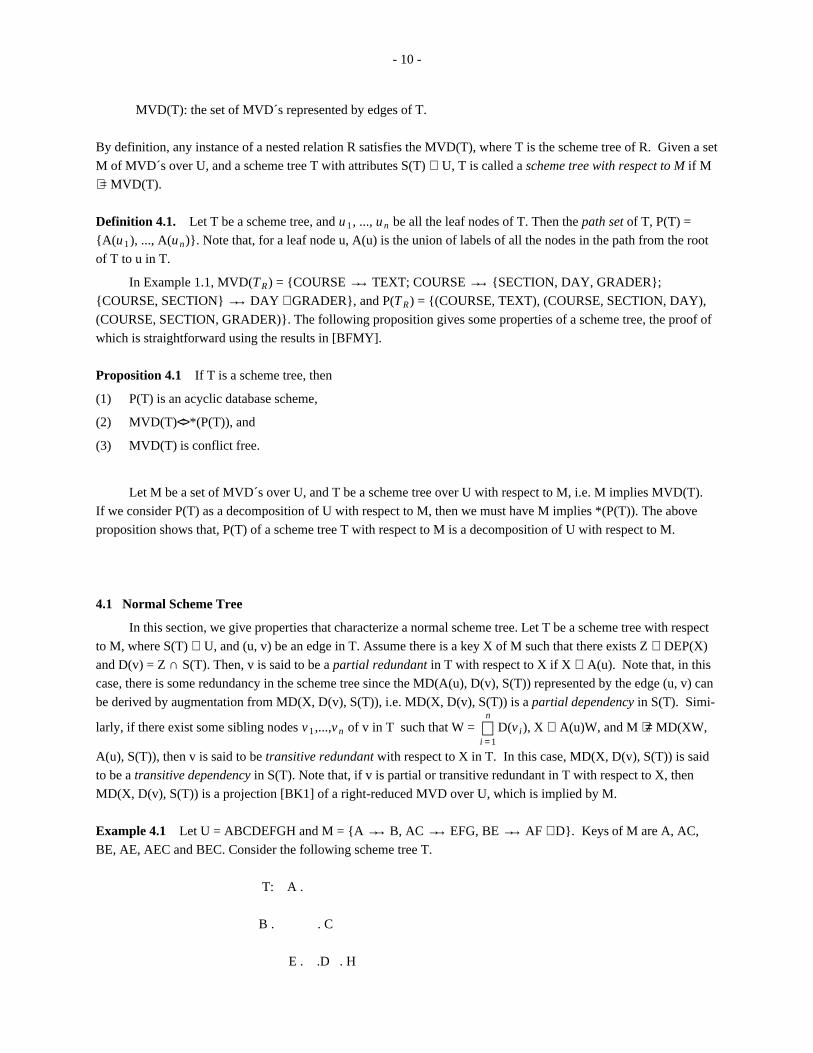
Example 4.1 Let U = ABCDEFGH and M = {A → → B, AC → → EFG, BE → → AF D}. Keys of M are A, AC,

BE, AE, AEC and BEC. Consider the following scheme tree T.

T: A .

B . . C

E . .D . H

- 11 -

F. .G

F is partial redundant with respect to AE, since for the edge (E, F) in T, M = (AE → → F) and AE ⊂ A(E) = ACE. D

is transitive redundant with respect to AE, since for the edge (C, D), M = (AE → → D) and AE ⊂ ACEFG but M ≠(AEFG → →AC).

A normal scheme tree does not have partial or transitive redundant nodes. The following example shows two

scheme trees without any partial or transitive nodes but one is preferred to the other.

Example 4.2. Let U = ABCEF M = {AB → → CE, BC → → F}. AB and BC are both essential keys. Consider the

following scheme trees.

T 1: AB . T 2: AB

F. .C F. .E

.E .C

T 1 and T 2 have no redundant nodes and M = MVD(T 1), M = MVD(T 2). However, the essential key BC is

separated by E in T 2 while no essential key is separated in T 1 . In this example, T 1 is a normal scheme tree while T 2

is not. The reason why T 1 is better than T 2 will be clear when we consider scheme trees which represent MVD´s

embedded in U.

In order to avoid anomalies in scheme trees (such as in T 2 of above example), we define a set of attributes

called a fundamental key. Let M be a set of MVD´s * on U and V ⊆ U. The set of fundamental keys on V, denoted

FK(V), is defined as follows.

FK(V) = {V ∩ X X ∈ LHS(M) and V ∩ X ≠ ∅, and no Y ∈ LHS(M) s.t. X ∩ V ⊃ Y ∩ V ≠ ∅}.

Obviously, FK(V) = ∅ iff for each X ∈ LHS(M), X ∩ V = ∅. Now we can define a normal scheme tree.

Definition 4.2. A scheme tree T is said to be normal with respect to a set of MVD´s M, if

(C1) M = MVD(T),

(C2) for each edge (u, v) of T, MD(A(u), D(v), S(T)) is left and right-reduced,

(C3) for each node u in T, there is no key X of M such that u is transitive redundant with respect to X, and

(C4) the root of T is a key, and for each other node u in T, if FK(D(u))≠ ∅ then u ∈ FK(D(u)).

In the above conditions, C1 is implied since T is a scheme tree with respect to M, C2 excludes partial depen-

dencies, and C3 excludes transitive dependencies in T. The condition C4, refers to the situation in Example 4.2.

Note that, T 1 in this example satisfies C4 but T 2 does not since for the node E, D(E) = CE, FK(CE) = {C} but E ∈/FK(CE). The proposition 4.3, below, shows that the path set P(T) of a normal scheme tree T with respect to a con-

flict free set of MVD´s M is in W4NF (i.e. in 4NF if we consider only those MVD´s that are not embedded). First,

we show the following lemma.__________________* Note that, we use M to denote minimal cover of a set of MVD´s.

- 12 -

Lemma 4.2. Let T be a normal scheme tree with respect to a set M of MVD´s, P be a path in T, and L be the leaf

of P. If there is a key X ⊂ P such that X splits P, then L ⊆ X.

Proof: Let X ⊂ P be a key of M such that L ⊆/ X. If L ∩ X ≠ ∅, then FK(D(L)) = FK(L) ≠ ∅ and L ∈/ FK(L), which

contradicts to C4 in the definition 4.2. Therefore, we have L ∩ X = ∅. Let A = A(F(L)), then X ⊆ A, and since T is

a normal scheme tree, MD(A, L, S(T)) is left- and right-reduced, so there is a V ∈ DEP(X) such that V ⊇ L. Let V A

= V ∩ A, then XV A → → XV AV_ _

, where V_ _

= U − XV, i.e. MD(XV A , XV A(V_ _

∩ S(T)), S(T)). Since MD(A, L, S(T))

and XV A(V_ _

∩ S(T)) ⊇ A, we have MD(XV A(V_ _

∩ S(T)), L, S(T)). Therefore, by the transitivity rule, we get

MD(XV A , L − XV A(V_ _

∩ S(T)), S(T)), i.e. MD(XV A , L, S(T)). If X splits P, then XV A ⊂ A, i.e. MD(A, L, S(T)) is

left-reducible. A contradiction.

Proposition 4.3. If M is conflict free then the path set P(T) of a normal scheme tree with respect to M is in W4NF.

Proof: By Proposition 4.1, M = *(P(T)), therefore, we need only show that for each P in P(T), P is in W4NF.

Assume not. Then there is a key X and a W ∈ RDEP(X) such that XW ⊂ P. Let u be the lowest node in P such that u

∩ W ≠ ∅, and L be the leaf of P, by Lemma 4.2, L ⊆ X, so u ≠ L. By Lemma 3.3 (4), there is an essential key X´ ⊆X such that L ∩ X´ ≠ ∅, i.e. D(u) ∩ X´ ≠ ∅. Therefore, FK(D(u)) ≠ ∅, that means there is an essential key Y such

that u = D(u) ∩ Y ∈ FK(D(u)). W ∩ u ≠ ∅ and u ⊆ Y imply that Y ∩ W ≠ ∅. Hence, by Lemma 3.3 (2), Y splits

XW ⊂ P, and, by Lemma 4.2, L ⊆ Y, which contradicts that u = D(u) ∩ Y.

4.2 Normal Scheme Forest

The above discussions show that, if T is a normal scheme tree over U with respect to M then T is a good

representation for instances of U satisfying M. However, it is not always possible to obtain such a normal scheme

tree, even when M is conflict free. Instead, given U and M, we can obtain a set of normal scheme trees.

Example 4.3 For U = ABCDEFG and M = {A → → B, AC → → EFG, BE → → AF D}, given in Example 4.1 there

is no single normal scheme tree. However, F = {T 1 , T 2} is a set of normal scheme trees over U with respect to M,

where

T 1: A. T 2: AE.

B. .C F. .D

E. .H

G.

Definition 4.3. Let M be a set of MVD´s over U, and F = {T 1 , ..., T n} be a set of normal scheme trees. F is a nor-

mal scheme forest (NSF) with respect to M if

(1) S(F) =i = 1∪

n

S(T i) = U, and

(2) M = *(S(T 1), ..., S(T n)).

In Example 4.3, F = {T 1 , T 2} is an NSF. Note that, any 4NF relation scheme can be structured in the form of

a normal scheme tree, which consists of a single path. Thus, any 4NF decomposition of U with respect to M is a

- 13 -

trivial NSF decomposition. However, in our context, we are interested in finding an NSF of scheme trees which are

not necessarily single paths. In the next section, we present a decomposition algorithm to obtain a normal scheme

forest with respect to a given set M of MVD´s over U. Properties of a normal scheme forest are given in section 6.

5. Decomposition Algorithm

The decomposition starts by decomposing U into a scheme tree T and then decomposes T into a set of normal

scheme trees T 1 , ..., T n . Informally, an intermediate scheme tree manipulated by the algorithm, is called a semi-

normal tree.

Definition 5.1 A scheme tree T is a semi-normal tree with respect to M, if

(1) M = MVD(T)

(2) For each edge (u, v) in T, MD(A(u), D(v), S(T)) is right-reduced.

(3) For each inner node* u in T, u ∈ FK(D(u)).

By comparing the above definition with the definition 4.2, it follows that a normal scheme tree is a semi-

normal tree, but the reverse is not true, as illustrated by the following example.

Example 5.1 Let U = ABCDE, M = {A → → B, C → → D, C → → E}.

T 1: A. T 2: A.

B. .CDE B. .C

D. . E

Scheme trees T 1 and T 2 are both semi-normal, but not normal scheme trees. T 1 is not a normal scheme tree since

for the node CDE, D(CDE) = CDE, FK(D(CDE)) ≠ ∅, but CDE is not in FK(D(CDE)). T 2 is not a normal scheme

tree since the MVD AC→ →D represented by the edge (C, D) is not left reduced.

Let T be a semi-normal scheme tree with respect to M, and V be a leaf of T. Then V is said to be decompos-

able if there is a V 0 in FK(V) such that V 0 ⊂ V. (In fact, if V is decomposable then FK(V)≠∅ and for any V 0 in

FK(V), V 0 ⊂ V). A semi-normal tree is nondecomposable if no leaf in T is decomposable. A node in semi-normal

tree T is redundant if it is partial redundant or transitive redundant with respect to a key X of M. A semi-normal tree

is nonredundant if it has no redundant nodes. In Example 5.1, T 1 is decomposable since FK(CDE) = {C}⊂CDE, but

nonredundant. T 2 is nondecomposable but redundant since nodes D and E are both partial redundant with respect to

the key C. The following proposition directly follows from definitions.

Proposition 5.1. If a semi-normal tree T with respect to M is nonredundant, nondecomposable, and the root of T is

a key, then T is a normal scheme tree.

5.1. Basic Procedures

Given a set M of MVD´s over U, a single node, labeled U, is a semi-normal tree. In this section, we give two

procedures; the first one decomposes a semi-normal tree into a nondecomposable semi-normal tree; and the second__________________* An inner node is a node which is neither the root nor a leaf in T.

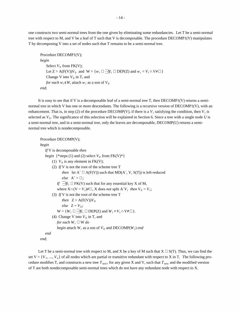
- 14 -

one constructs two semi-normal trees from the one given by eliminating some redundancies. Let T be a semi-normal

tree with respect to M, and V be a leaf of T such that V is decomposable. The procedure DECOMP1(V) manipulates

T by decomposing V into a set of nodes such that T remains to be a semi-normal tree.

Procedure DECOMP1(V);

begin

Select V 0 from FK(V);

Let Z = A(F(V))V 0 and W = {w i ———

V i ∈ DEP(Z) and w i = V i ∩V≠ ∅}

Change V into V 0 in T, and

for each w i εW, attach w i as a son of V 0

end;

It is easy to see that if V is a decomposable leaf of a semi-normal tree T, then DECOMP1(V) returns a semi-

normal tree in which V has one or more descendants. The following is a recursive version of DECOMP1(V), with an

enhancement. That is, in step (2) of the procedure DECOMP(V), if there is a V i satisfying the condition, then V i is

selected as V 0 . The significance of this selection will be explained in Section 6. Since a tree with a single node U is

a semi-normal tree, and in a semi-normal tree, only the leaves are decomposable, DECOMP(U) returns a semi-

normal tree which is nondecomposable.

Procedure DECOMP(V);

begin

If V is decomposable then

begin {*steps (1) and (2) select V 0 from FK(V)*}

(1) V 0 is any element in FK(V);

(2) If V is not the root of the scheme tree T

then let A´ ⊆ A(F(V)) such that MD(A´, V, S(T)) is left-reduced

else A´ = ∅;

If ———

V i ∈ FK(V) such that for any essential key X of M,

where X∩(V − V i)≠∅, X does not split A´V i then V 0 = V i ;

(3) If V is not the root of the scheme tree T

then Z = A(F(V))V 0

else Z = V 0;

W = {W i ———

V i ∈ DEP(Z) and W i = V i ∩V≠ ∅}.

(4) Change V into V 0 in T, and

for each W i ∈ W do

begin attach W i as a son of V 0 and DECOMP(W i) end

end

end;

Let T be a semi-normal tree with respect to M, and X be a key of M such that X ⊂ S(T). Thus, we can find the

set V = {V 1 , ..., V n} of all nodes which are partial or transitive redundant with respect to X in T. The following pro-

cedure modifies T, and constructs a new tree T new , for any given X and V, such that T new and the modified version

of T are both nondecomposable semi-normal trees which do not have any redundant node with respect to X.

- 15 -

Procedure NEWTREE(X, V, T, T new)

begin

Let T new be a tree with only one node labeled X;

for each V i in V do

begin delete D(V i) from T, and

attach D(V i) as a subtree of X in T new end

end;

To show the correctness of NEWTREE(X, V, T, T new), we need the following lemmas.

Lemma 5.2. Let W = W 0W 1 ...W k be a dependent of both X and Y with respect to M. Then, if W i ∈ DEP(XW 0)

then W i ∈ DEP(YW 0) for 1 ≤ i ≤ n, where W i , X, and Y are subsets of U.

Proof: Let W_ _

= U − W, then XW 0 ⊆ W_ _

W 0 . Y → → W implies Y → → W_ _

, therefore, YW 0 → → W_ _

W 0 . Since XW 0 → →W i , W

_ _W 0 → → W i , thus, YW 0 → → W i , for i=1,...k. If YW 0 → → W i is right-reducible, for some 1 ≤ i ≤ k, then, simi-

larly, XW 0 → → W i is right-reducible, which is a contradiction.

Lemma 5.3. If T is a nondecomposable semi normal tree, then both T and T new returned by NEWTREE(X, V, T,

T new) are both nondecomposable semi normal trees.

Proof: Let T´ be T before it was modified. Obviously, T is a nondecomposable semi normal tree, since T´ is a non-

decomposable semi normal tree. Lemma 5.2 guarantees that T new satisfies the first two conditions of a semi normal

tree. The root of T new is X, which is a key of M, and each inner node and leaf in T new appears the same as it does in

T´. Thus, it follows that T new is a nondecomposable semi normal tree.

5.2. Algorithm

Given a set M of MVD´s on U, a normal scheme forest can be constructed as follows: Let F = {T 1} where T 1

is the nondecomposable semi-normal tree constructed by DECOMP(U). For each key X of M, find the set V of all

nodes in some T i ∈ F which are redundant with respect to X, and call NEWTREE (V, X, T i , T j) to construct a new

tree T j such that both T i and T j are nondecomposable semi-normal trees without any redundant nodes with respect

to X. While considering the keys of M we use a p-ordering [L1] (i.e. an ordering X 1 , ..., X n where X i⊆X j only if i ≤j for 1 ≤ i, j ≤ n. Obviously, p-ordering of a set of keys is not unique). A p-ordering of keys, together with Lemma

3.1 (1), guarantees that before calling NEWTREE (X, V, T i , T j), for any key X i of M, if there is a T i such that

X⊂S(T i), then T i is the only tree containing X among the trees constructed so far. Let F = {T 1 , ..., T k}, after all keys

of M are processed as described above. Then each T i ∈ F is a nondecomposable semi-normal tree without any

redundant nodes. Thus, by Proposition 5.1, F is a set of normal scheme trees with respect to M. Since each attribute

in U is in at least one tree of F, S(F) = U. In order to show, M = *(S(T 1), ..., S(T k)), consider the case with k = 2,

where T 2 is constructed from T 1 by NEWTREE (X, V, T 1 , T 2). Let T 1´ denote the only scheme tree, i.e. T 1 , before

T 2 is constructed. Then, by construction, S(T 1)∩S(T 2) = X. Since S(T 2) − S(T 1) = W =i = 1∪

n

D(W i), where V = {W 1 ,

..., W n}, and X → → W in S(T 1´) = U, M = *(S(T 1), S(T 2)). Since {T 1 , ..., T n} is obtained by repeated applications

of this procedure, it follows that M = *(S(T 1), ..., S(T k)). Thus, Algorithm D, correctly produces a normal scheme

forest F with respect to M.

- 16 -

Algorithm DInput: A set of attributes U and a set of MVD´s M on U.

Output: A normal scheme forest F = {T 1 , ..., T j}.

(1) Calculate all keys of M [OY].

(2) T 1 := DECOMP(U); j := 1;

(3) Let X 1 , ..., X n be a p-ordering of keys of M.

for i := 1 to n do

begin if X i ⊂ S(T k) for some 1 ≤ k ≤ j then

begin V := ∅for each node W in T k such that —

——

Z ∈ DEP(X i) and D(W) = Z ∩ S(T k) do

if W is redundant with respect to X i or (Z ∈ EDEP(X i) and Z ∈/ EDEP(A(F(W)))

then V:=V ∪ {W};

if V ≠ ∅ then begin j := j + 1; and NEWTREE(X i , V, T k , T j) end

end

end;

4. Output F = {T 1 , ..., T j};

Note that, in step (3), the set V constructed for the key X i may contain a node W ∈ T k where W is not redun-

dant in T k with respect to X i . In this case, W is the part of an essential dependent of X i in S(T k), but not of A(F(W)),

and it seems better to attach W as a descendant of X i in T j even though W is not redundant in T k with respect to X i .

The correctness of Algorithm D, with this enhancement, follows from the discussions above. The following exam-

ple, illustrates Algorithm D.

Example 5.2. Let U = ABCDEFGHIJ, and M = {A → → B, B → → E F, AC → → DJH, AJ → → H, AD → → J G}.

M is a minimal cover. The set of essential keys of M is LHS(M) = {A, B, AC, AJ, AD}, and the only nonessential

key is ACJ. Suppose we choose a p-ordering A, B, AC, AD, AJ, ACJ of keys. The scheme tree T 1 obtained in step

(1) is

T 1 A .

. . . . C

B E F

D . . .

I G

. .

J H

Since E and F are redundant in T 1 with respect to the key B, NEWTREE(B, {E, F}, T 1 , T 2) modifies T 1 and con-

structs T 2 as follows:

- 17 -

T 1: A. T 2: B.

B. .C E. . F

D . . .

I G

J . .H

Similarly, after all the keys are considered in step (3), the resulting normal scheme forest is F = {T 1 , T 2 , T 3 , T 4},

where

T 1: A. T 2: B. T 3: T 4:

B. .C E. .F AD. AJ.

D . . I J. . G H.

In this example, the normal scheme forest produced by the algorithm is the same if keys AD and AJ are inter-

changed in the p-ordering used in step (3). However, T 1 produced in step (1) depends on the ordering of essential

keys in FK(V) used in decomposing a node V of an intermediate semi-normal tree. In the next section, we present

properties of a normal scheme forest produced by Algorithm D.

6. Properties of Decomposition

Given a set of MVD´s M over U, let F = {T 1 , ..., T n} be an NSF decomposition obtained by Algorithm D. By

definition, for each T i ∈ F, M = MVD(T i). However, there may be some other MVD´s implied by M but not

represented by a T i in F. To capture some of these dependencies we define a construction graph J(F) for F as a con-

nected graph (F, E), where the normal scheme forest F is the set of vertices and E is an ordered set of directed edges.

An edge e = (T i , T k) ∈ E iff T k is constructed from T i by the procedure NEWTREE (X, V, T i , T k) (in step 3), and

the label of e is the root of T k , i.e. L(e) = X. The order of edges is determined by the order T i´s are constructed, i.e.

for e i = (T s , T k) and e j = (T x , T m), i<j iff T k is constructed before T m.

Example 6.1. For F = {T 1 , T 2 , T 3 , T 4} in Example 5.2, the construction graph J(F) is as follows.

B

T 1 . .T 2

e 1

AD e 2

AJ

T 3 . .T 4

e 3

Obviously, for any F constructed by Algorithm D, J(F) is a tree.

- 18 -

For the MVD´s represented by edges of J(F), we need some notations. Let DS(T i), where T i ∈ F, denote the

set of all attributes in trees that are descendants of T i in F, including T i . For each e i ∈ F, let AT(e i) denote the set of

all attributes in the connected component containing e i after all edges e j where j<i are deleted from J(F). The MVD

represented by an edge e = (T i , T k) is MVD(e) = MD(L(e), DS(T k) − L(e), AT(e)). The set of MVD´s represented

by F = {T 1 , ..., T n} is MVD(F) = { MVD(e i) e i ∈ J(F)} ∪ (i = 1∪

n

MVD(T i)).

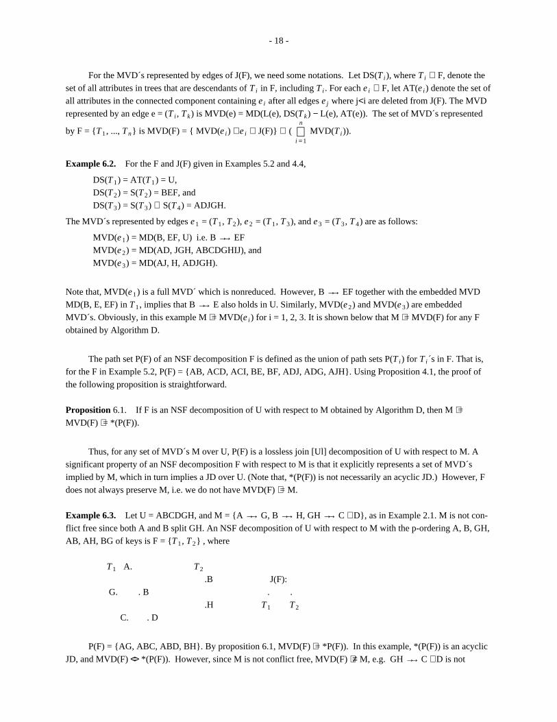
Example 6.2. For the F and J(F) given in Examples 5.2 and 4.4,

DS(T 1) = AT(T 1) = U,

DS(T 2) = S(T 2) = BEF, and

DS(T 3) = S(T 3) ∪ S(T 4) = ADJGH.

The MVD´s represented by edges e 1 = (T 1 , T 2), e 2 = (T 1 , T 3), and e 3 = (T 3 , T 4) are as follows:

MVD(e 1) = MD(B, EF, U) i.e. B → → EF

MVD(e 2) = MD(AD, JGH, ABCDGHIJ), and

MVD(e 3) = MD(AJ, H, ADJGH).

Note that, MVD(e 1) is a full MVD´ which is nonreduced. However, B → → EF together with the embedded MVD

MD(B, E, EF) in T 1 , implies that B → → E also holds in U. Similarly, MVD(e 2) and MVD(e 3) are embedded

MVD´s. Obviously, in this example M = MVD(e i) for i = 1, 2, 3. It is shown below that M = MVD(F) for any F

obtained by Algorithm D.

The path set P(F) of an NSF decomposition F is defined as the union of path sets P(T i) for T i´s in F. That is,

for the F in Example 5.2, P(F) = {AB, ACD, ACI, BE, BF, ADJ, ADG, AJH}. Using Proposition 4.1, the proof of

the following proposition is straightforward.

Proposition 6.1. If F is an NSF decomposition of U with respect to M obtained by Algorithm D, then M =MVD(F) = *(P(F)).

Thus, for any set of MVD´s M over U, P(F) is a lossless join [Ul] decomposition of U with respect to M. A

significant property of an NSF decomposition F with respect to M is that it explicitly represents a set of MVD´s

implied by M, which in turn implies a JD over U. (Note that, *(P(F)) is not necessarily an acyclic JD.) However, F

does not always preserve M, i.e. we do not have MVD(F) = M.

Example 6.3. Let U = ABCDGH, and M = {A → → G, B → → H, GH → → C D}, as in Example 2.1. M is not con-

flict free since both A and B split GH. An NSF decomposition of U with respect to M with the p-ordering A, B, GH,

AB, AH, BG of keys is F = {T 1 , T 2} , where

T 1 A. T 2

.B J(F):

G. . B . .

.H T 1 T 2

C. . D

P(F) = {AG, ABC, ABD, BH}. By proposition 6.1, MVD(F) = *P(F)). In this example, *(P(F)) is an acyclic

JD, and MVD(F) <=> *(P(F)). However, since M is not conflict free, MVD(F) ≠ M, e.g. GH → → C D is not

- 19 -

represented by F, although AB → → C D G H implied by M, but not by M − {GH → → C D}, is also implied

by MVD(F).

Another significance of this example is that P(F) is a 4NF decomposition of U with respect to M, and it is easy

to verify that for this example, any F´ produced by Algorithm D satisfies P(F) = P(F´) This is because of the

enhancement in Step (2) of the procedure DECOMP(V). That is, since GH is split by A and B, the essential key GH

is never used to decompose a node V which contains A or B. Lien [L1] also observed that his decomposition algo-

rithm produces a 4NF decomposition for this example if a p-ordering in which GH precedes both A and B is used;

and fails to produce a 4NF decomposition otherwise. This is because, in [L1] only the keys in LHS(M), but not all

the keys [OY], are used for the decomposition.

In the above example, P(F) = {AG, ABC, ABD, BH} is a lossless 4NF decomposition of U with respect to M,

but it is not dependency preserving. It is easy to see that P(F) is not an SFNF decomposition of U with respect to M

[BK2], since ABC (and also ABD) are split by GH → → C D. The next proposition shows that if M is conflict free,

then for any F produced by Algorithm D, P(F) is a unique dependency preserving SFNF decomposition of U.

Proposition 6.2 Let F be an NSF decomposition of U with respect to M obtained by Algorithm D, and M be a

conflict free set of MVD´s over U. Then

(1) P(F) is a unique SFNF decomposition of U,

(2) M <=> MVD(F) <=> *(P(F)), and

(3) P(F) is acyclic.

In order to show this proposition we need some lemmas. Algorithm D constructs F = {T 1 , T 2 , ...,T J} one

after another by calling NEWTREE. Let T i´ be the T i in F when it was just constructed in the algorithm. Obviously,

T i´ may not be the same as T i , since some nodes may be deleted later. By Lemma 5.3, T i´, 1 ≤ i ≤ J, is a nondecom-

posable semi normal tree. Thus, T 1´ is the nondecomposable semi normal tree obtained from DECOMP(U) in step 2

of the algorithm, and for any inner or leaf node v in T i , 1 ≤ i ≤ J, there is a corresponding node v 1 in T 1´ such that v 1

= v.

Lemma 6.3. Let F = {T 1 , T 2 ,...T J} be an NSF decomposition obtained by Algorithm D, e = <u, v> be an edge in

T i , 1 ≤ i ≤ J, and v 1 be the node corresponding to v in T 1´, A(u) and D´(v 1) be defined as A(u) and D(v 1) in T i and

T 1´ respectively. Then A(u) → → D´(v 1), and it is a left- and right-reduced MVD.

Proof: There is a sequence of trees T k1 , T k2 , ..., T kn in F such that T k1 = T 1 , T kn = T i , and T k j is constructed from

T k( j − 1 ) , for 2 ≤ j ≤ n. For 1 ≤ j ≤ n, let T j´ be the T k j when it was just constructed, and e j = <u j , v j> be an edge in

T j´ such that v j is the node corresponding to v, i.e. v j = v. A(u j), D(v j), A´(u j), and D´(v j) are defined in T k j and T j´

respectively. Obviously, A(u j) = A´(u j), D(v j) ⊆ D(v j), and D(v j) = D´(v j) ∩ S(T k j). First we show that, for any 1 ≤j ≤ n, A(u j) → → D´(v 1) is right-reduced by induction on j.

Basis: j = 1, it is trivial.

Induction step: Assume A(u n − 1) → → D´(v 1) is right-reduced. Let T ́ ´ be the T k(n − 1 ) just before T n´ was con-

structed by calling NEWTREE(X, V, T ́ ´, T n´). Thus, e n − 1 = <u n − 1 , v n − 1> is also in T ́ ´. Let D ́ ´(v n − 1) be D(v n − 1)

defined in T ́ ´, then D ́ ´(v n − 1) = D(v n) ⊆ D´(v n − 1). By Lemma 5.3, T ́ ´ is a semi normal tree, so MD(A(u n − 1), D ́ ´(v n − 1),

S(T ́ ´)) is right-reduced. Since T n´ is constructed from T ́ ´, by Lemma 5.2, MD(A(u n), D ́ ´(v n − 1), S(T ́ ´)) is also right-

reduced. These two MVD´s are projections of some full MVD´s implied by M on S(T ́ ´), i.e. there exist D n − 1 ∈DEP(A(u n − 1)) and D n ∈ DEP(A(u n)) such that D ́ ´(v n − 1) = D n − 1 ∩ S(T ́ ´) and D ́ ´(v n − 1) = D n ∩ S(T ́ ´). By Lemma

- 20 -

3.2, D n − 1 = D n . By the induction assumption, D´(v 1) ∈ DEP(A(u n − 1)) and D n − 1 ∩ D´(v n − 1) ≠ ∅, thus D´(v 1) =

D n − 1 = D n . That is D´(v 1) ∈ DEP(A(u n)).

T kn is a normal scheme tree, so MD(A(u n), D(v n), S(T kn)) is left- and right-reduced, and obviously, this MVD

is the projection of the MVD A(u n) → → D´(v 1) on S(T kn). It follows that A(u n) → → D´(v 1) is left- and right-

reduced.

Let M be a conflict free set of MVD´s, Z, V be sets of attributes such that Z→ →V is left- and right-reduced, M

does not split Z and FK(V) ≠ ∅, and K = {Y i Y i is an essential key and Y i ∩ V≠∅}. A binary relation "<" is

defined on K as follows.

Y i<Y j iff ZY i is split by Y j but not by any Y j´ ⊂ Y j in K.

Then we have the following lemma.

Lemma 6.4. "<" is irreflexive, antisymmetric, and transitive.

Proof: (1) "<" is irreflexive, i.e. Y i </ Y i . Y i does not split Z, so Y i does not split Y iZ.

(2) "<" is antisymmetric. Showing that Y i < Y j => Y i does not split ZY j is sufficient. Assume not, i.e. Y i<Y j

and Y i splits ZY j . Y i<Y j implies that there exists a V j ∈ DEP(Y j) such that Z j = V j ∩ Z ≠ ∅ and V j ∩ Y i = ∅. Y i

splits ZY j implies that there exists a V i ∈ DEP(Y i) such that Z i = V i ∩ Z ≠ ∅ and V i ∩ Y j = ∅, and Y j − Y i ≠ ∅,

i.e. Y i ∩ Y j ⊂ Y j . We claim that Z i ∩ Z j ≠ ∅, i.e. V i ∩ V J ≠ ∅, otherwise, since Y i does not split Z, Z j ⊆ Y i . This

implies Y j splits Y i , which is a contradiction. Therefore, by Lemma 3.2 and 2.4, V i = V j ∈ DEP(Y i ∩ Y j). That

means Y i ∩ Y j splits ZY i , and, by Lemma 3.4 (1), there is an essential key Y´ ⊆ (Y i ∩ Y j) such that Y´ splits ZY i ,

and, by Lemma 3.4 (2), Y´ ∈ K, which contradicts that Y i<Y j .

(3) "<" is transitive, i.e. Y i < Y j and Y j < Y k => Y i < Y k . Y i<Y j implies that DEP(Y j) = {V j1 , V j2 , ...},

where Z ⊆ Y jV j1 , Z ∩ V j1≠∅, Y i ⊆ Y jV j2 , and Y i ∩ V j2 ≠ ∅. Y j < Y k implies that DEP(Y k) = {V k1 , V k2 , ...},

where Z ⊆ Y k V k1 , Z ∩ V k1 ≠ ∅, Y j ⊆ Y k V k2 , and Y j ∩ V k2 ≠ ∅.

First, we show that Y k splits ZY i . If V k1 ∩ Y i = ∅ and Y i − Y k ≠ ∅, then Y k splits ZY i . Suppose Y i − Y k =

∅, i.e. Y i ⊆ Y k . Then Y j splits ZY k since Y j splits ZY i , which contradicts to Y j < Y k . Now, we need to show V k1 ∩Y i = ∅. Let Y i1 = Y i ∩ Y j and Y i2 = Y i ∩ V j2 , since Y i ⊆ Y jV j2 , Y i = Y i1Y i2 . Y j ∩ V k1 = ∅ implies Y i1 ∩ V k1 = ∅.

The fact that Y k → → Y kV k2 and Y kV k2 → → V j2 implies Y k → → (V j2 − Y kV k2), i.e. Y k → → (V j2 − V k2). Y k → → (V j2

− V k2) and Y k → → V k1 implies Y k → → (V k1 − (V j2 − V k2)), i.e. Y k → → (V k1 − V j2). Since V k1 ∈ DEP(Y k), (V k1 −V j2) = V k1 , i.e. V j2 ∩ V k1 = ∅, so Y i2 ∩ V k1 = ∅. It follows that Y i ∩ V k1 = ∅. Thus, Y k splits ZY i .

Then, we show that no Y´ ⊂ Y k in K such that Y i < Y´. Assume not, i.e. there is a Y´ ⊂ Y k in K such that Y i <Y´. Y i < Y´ implies that DEP(Y´) = {V 1´, V 2´, ...}, where, Z ⊆ Y´V 1´, Z ∩ V 1´ ≠ ∅, Y i ⊆ Y´V 2´, and Y i ∩ V 2´ ≠∅. Y j < Y k implies that Y´ does not split ZY j , so Y jZ ⊆ Y´V 1´. Similarly, we have DEP(Y j) = {V j1 , V j2 , ...}, where,

Y kZ ⊆ Y jV j1 , Z ∩ V j1 ≠ ∅, Y i ⊆ Y jV j2 , and Y i ∩ V j2 ≠ ∅. Thus, V 2´ ∩ Y j = ∅, V j2 ∩ Y´ = ∅. If we can show that

V 2´ ∩ V j2 ≠ ∅, then, by Lemma 3.2 and 2.4, V 2´ = V j2 ∈ DEP(Y j ∩ Y´). So, Y j ∩ Y´ splits ZY i , bu Lemma 3.4 (1),

there is an essential key X ⊆ (Y j ∩ Y´) such that X splits ZY i . Y i < Y j and Y i < Y´ implies that Y´ ⊆/ Y j , i.e. Y j ∩Y´ ⊂ Y´. Therefore, X ⊂ Y´, and, by Lemma 3.4 (2), X is in K. Contradiction to Y i < Y´.

Now, we show that V 2´ ∩ V j2 ≠ ∅. Let A = V 2´ ∩ Y i , B = V j2 ∩ Y i . We have shown that A and B are

nonempty. Suppose A ∩ B = ∅, the fact that Y j → → V j2 and Y j does not split Y i implies that A ⊆ Y j , i.e. Y j ∩ V 2´ ≠∅, which contradicts that Y jZ ⊆ Y´V 1´.

Lemma 6.5. Let M be a conflict free set of MVD´s, Z, V be sets of attributes such that Z → → V is left- and right-

reduced. If M does not split Z and FK(V) ≠ ∅, then there exists an X 0 in FK(V) such that M does not split ZX 0 .

Proof: Let K = {Y i Y i is an essential key and Y i ∩ V ≠ ∅}. A binary relation "<" is defined on K as follows.

- 21 -

Y i < Y j iff ZY i is split by Y j but not by any Y j´ ⊂ Y j in K.

By Lemma 6.4, "<" is irreflexive, antisymmetric, and transitive on K, thus, there exists at least one Y in K such that

for any Y´ in K, Y </ Y´, i.e., no Y´ in K splits ZY. By Lemma 3.4, M does not split ZY ⊇ ZX 0 for some X 0 in

FK(V).

Lemma 6.6. Let F be an NSF decomposition of U with respect to M obtained by Algorithm D. If M is conflict free

then any path p in P(F) is nondecomposable with respect to M.

Proof: Refer to Algorithm D and the procedure DECOMP. Let T 1´ be the nondecomposable semi normal tree

returned by DECOMP(U) in step 2 of the algorithm. Lemma 6.5 guarantees that the selecting condition in step 2 of

DECOMP is always satisfied. Thus, for any edge e = <u 1 , v 1> in T 1´, there exists an X ⊆ A(u 1) in T 1´ such that X

→ → D(v 1) is left- and right-reduced and, X is not split by any essential key Y, where Y ∩ D(v 1) ≠ ∅. Let e = <u, v>be any edge in p, then there exists an edge e = <v 1 , v 1> in T 1´ such that v 1 is the corresponding node of v, i.e. v 1 =

v. By Lemma 6.3, A(u) → → D(v 1) is left- and right-reduced, and by Lemma 3.3 (1), A(u) = X, and D(v) ⊆ D(v 1).

Therefore, A(u) is not split by any essential key Y, where Y ∩ D(v) ≠ ∅. Let L be the leaf of p, and A be A(F(L)) in

p. Assume p is decomposable with respect to M, then by Lemma 4.2 and 3.4 (1), there exists an essential key Z ⊇ L

and Z splits p, i.e. Z splits A, which is a contradiction.

Proof of Proposition 6.2:

(1) From Proposition 6.1, and Lemma 6.6, it follows that P(F) is a 4NF decomposition of U with respect to M.

Since M is conflict free, by Proposition 2.3, P(F) is unique and also in SFNF.

(2) >From (1) and Lemma 8.7 in [BFMY], M <=> *(P(F)). Thus from Proposition 6.1, it follows that

M <=> MVD(F) <=> *(P(F)).

(3) Follows from (2) and Theorem 3.4 in [BFMY].

Let M be a set of MVD´s over U, and F = {T 1 ,...,T n} be a normal scheme forest decomposition of U with

respect to M. If M is not conflict free, then the join dependencies implied by the decomposition, i.e.,

*(S(T 1),...,S(T n)) and *(P(F)) are not necessarily acyclic join dependencies. We conclude this section by an example

illustrating this situation.

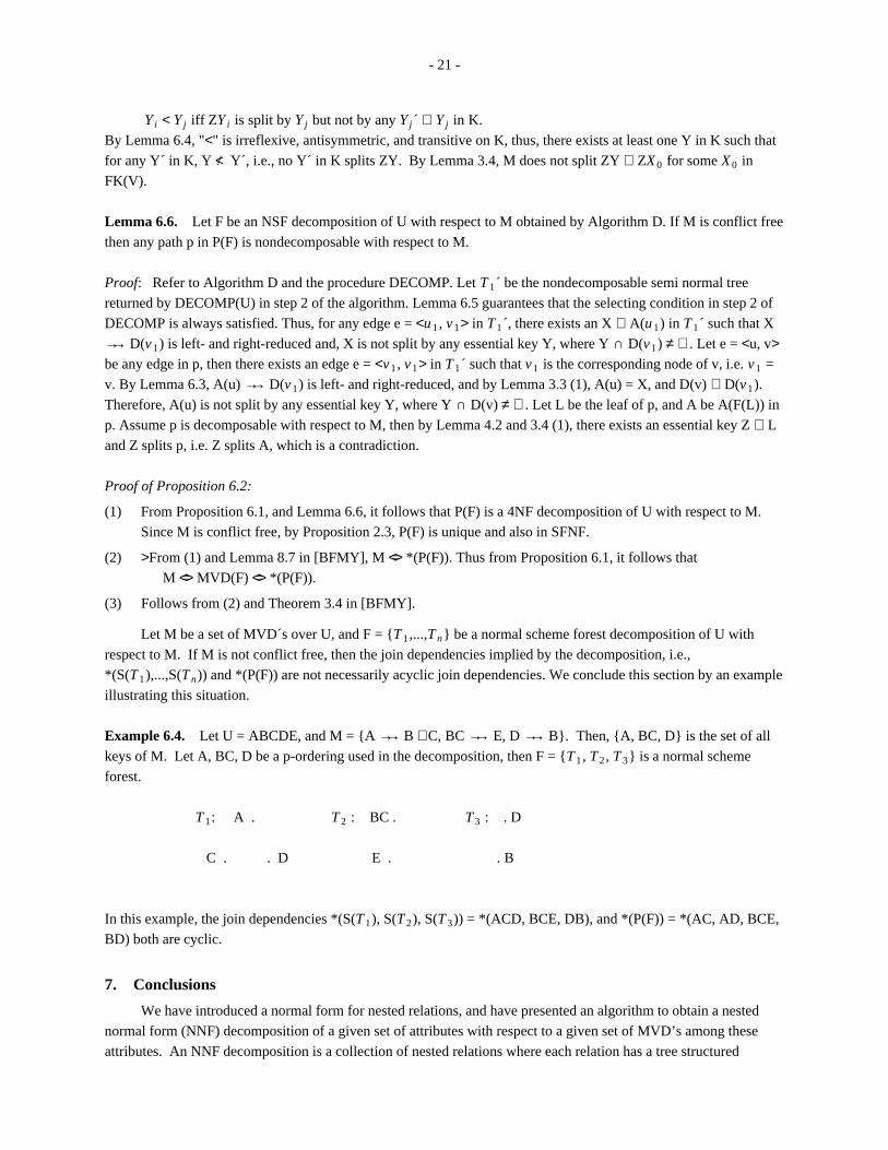
Example 6.4. Let U = ABCDE, and M = {A → → B C, BC → → E, D → → B}. Then, {A, BC, D} is the set of all

keys of M. Let A, BC, D be a p-ordering used in the decomposition, then F = {T 1 , T 2 , T 3} is a normal scheme

forest.

T 1: A . T 2 : BC . T 3 : . D

C . . D E . . B

In this example, the join dependencies *(S(T 1), S(T 2), S(T 3)) = *(ACD, BCE, DB), and *(P(F)) = *(AC, AD, BCE,

BD) both are cyclic.

7. Conclusions

We have introduced a normal form for nested relations, and have presented an algorithm to obtain a nested

normal form (NNF) decomposition of a given set of attributes with respect to a given set of MVD’s among these

attributes. An NNF decomposition is a collection of nested relations where each relation has a tree structured

- 22 -

scheme, called normal scheme tree. That is an NNF database scheme is a forest of normal scheme trees. One of the

objectives of NNF is to reduce redundancy. Moreover, since the normal scheme forest is structured with respect to

dependencies existing among attributes, the database scheme explicitly represents these dependencies. If the given

set M of MVD´s is conflict free, then any NNF decomposition is dependency preserving, i.e., the MVD´s

represented by the database scheme is equivalent to the existing MVD´s among attributes. Nevertheless, if M is not

conflict free, then the NNF database scheme represents a set of nontrivial MVD´s, that are implied by M. The NNF

decomposition of a set of attributes U with respect to any set M of MVD´s is a nonredundant and faithful (lossless)

decomposition of U. In a sense, the nested normal form decomposition can be considered as a formal way of design-

ing a hierarchical database by utilizing the MVD´s existing among attributes.

It has been argued [Sc] that the real world MVD´s are conflict free, and the desirable properties of conflict free

MVD´s have been discussed by several researchers [BFMY, L2]. The NNF decomposition also has more desirable

properties when the given set M of MVD´s is conflict free. We have shown that if M is conflict free, then the set of

root-to-leaf paths in a normal scheme forest is precisely the unique 4NF decomposition of the given set of attributes

with respect to M. This unique 4NF decomposition is also the Split Free Normal Form decomposition [BK2], which

is a new normal form with desirable properties.

For convenience we consider FD´s, in this paper, as their MVD counterparts as in [L1] in obtaining NNF

decomposition. Since an FD is more than an MVD, some of the semantic connections among attributes are not

represented in the set M of MVD´s with this formulation. Hence, not all of the semantic connections existing among

attributes in the form of FD´s and MVD´s are utilized in obtaining NNF. We are now investigating a normal form

for nested relations in the context of FD´s and MVD´s, by incorporating the results of [YO] into nested normal form

decomposition.

References

[AB] Abiteboul, S. and Bidoit, N., Non First Normal for Relations to Represent Hierarchically Organized

Data, Proc. ACM PODS, 1984 pp. 191-200.

[Ba] Bancilhon, F., et al.., Verso: A Relational Back End Data Base Machine, Proc. International Workshop

on Database Machine, San Diego, 1982.

[BBG] Beeri, C., Bernstein, P.A., and Goodman, N., A Sophisticate´s Introduction to Database Normalization

Theory, Proc. VLDB, 1978, pp. 113-123.

[BFH] Beeri, C., Fagin, R., and Howard, J., A Complete Axiomatization for FD´s and MVD´s, Proc. ACM

SIGMOD, 1977, pp. 47-61.

[BFMY] Beeri, C., Fagin, R., Maier, D. and Yannakakis, M., "On the Desirability of Acyclic Database Schemes",

JACM, July 1983, pp. 479-513.

[BK1] Beeri, C. and Kifer, M., Elimination of Intersection Anomalies from Database Schemes, Proc. ACM

PODS, 1983, pp. 340-351.

[BK2] Beeri, C. and Kifer, M., Comprehensive Approach to the Design of Relational Database Schemes, Proc.

VLDB, 1984, pp. 196-207.

[Co] Codd, E., A Relational Model for Large Shared Data Bank, Comm. ACM, June 1970, pp. 377-387.

[Fa] Fagin, R., Multivalued Dependencies and a New Normal Form for Relational Databases, ACM TODS,

Sept. 1977, pp. 262-278.

[FG] Fischer, P.C. and Gucht, D.V., Weak Multivalued Dependencies, Proc. ACM PODS, 1984, pp. 266-274.

[FT] Fischer, P.C. and Thomas, S.J., Operations for Non-First-Normal Form Relations, IEEE Computer

Software and Applications Conference, Oct. 1983, pp. 464-475.

- 23 -

[Ha] Hawryszkiewycz, I.T., Database Analysis and Design, SRA, 1984.

[JS] Jaeschke, G. and Scheck, H.J., Remarks on the Algebra of Nonfirst Normal Form Relations, Proc. ACM

PODS, 1982, pp. 124-138.

[KTT] Kambayashi, Y., Tanaka, K. and Takeda,K., Synthesis of Unnormalized Relations Incorporating more

meaning, Information Sciences, 1983.

[L1] Lien, Y.E., Hierarchical Schemata for Relational Databases, ACM TODS, March 1981, pp. 48-69.

[L2] Lien, Y.E., On the Equivalence of Database Models, JACM, April 1982, pp. 333-362.

[Ma] Maier, D., The Theory of Relational Databases, Computer Science Press, 1983.

[Sc] Sciore, E., Real World MVD´s, Proc. SIGMOD, 1981, pp. 121-132.

[OzOM] Ozsoyoglu, G., Matos, V., and Ozsoyoglu, Z.M., Extending Relational Algebra and Relational Calculus

with Set-Valued Attributes and Aggregate Functions, Technical Report, Department of Computer Sci-

ence, Case Western Reserve University, 1985.

[OO] Ozsoyoglu, Z.M. and Ozsoyoglu, G., An Extension of Relational Algebra for Summary Tables, Proc.

Statistical Database Workshop, 1983, pp. 202-211.

[OY] Ozsoyoglu, Z.M. and Yuan, L.Y., Reduced MVD’s and Minimal Covers, Technical Report, Department

of Computer Science, CES-84-06, Case Western Reserve University, 1984.

[RKS] Roth, M.A., Korth, H.F., and Silberschatz, A., Theory of Non-First-Normal Form Relational Databases.

TR-84-36, Department of Computer Science, University of Texas at Austin (December 1984).

[Ul] Ullman, J.D., Principles of Database Systems, Computer Science Press, Potomac, Maryland, 1983.

[YO] Yuan, L.Y. and Ozsoyoglu, Z.M., Unifying Functional and Multivalued Dependencies for Relational

Database Design, to appear in Proc. of the 5th ACM PODS, 1986.

[ZM] Zaniola, C., and Melkanoff, M.A., On the Design of Relational Database Schemata, ACM TODS,

March 1981, pp. 1-47.

View publication statsView publication stats