A New Nonparametric Estimate of theRisk-Neutral Density with Applicationsto Variance SwapsLiyuan Jiang1, Shuang Zhou1, Keren Li1, Fangfang Wang2 and Jie Yang1*

1Department of Mathematics, Statistics, and Computer Science, University of Illinois at Chicago, Chicago, IL, United States,2Department of Mathematical Sciences, Worcester Polytechnic Institute, Worcester, MA, United States

Estimates of risk-neutral densities of future asset returns have been commonly used forpricing new financial derivatives, detecting profitable opportunities, and measuring centralbank policy impacts. We develop a new nonparametric approach for estimating the risk-neutral density of asset prices and reformulate its estimation into a double-constrainedoptimization problem. We evaluate our approach using the S&P 500 market option pricesfrom 1996 to 2015. A comprehensive cross-validation study shows that our approachoutperforms the existing nonparametric quartic B-spline and cubic spline methods, as wellas the parametric method based on the normal inverse Gaussian distribution. As anapplication, we use the proposed density estimator to price long-term variance swaps, andthe model-implied prices match reasonably well with those of the variance futuredownloaded from the Chicago Board Options Exchange website.

Keywords: pricing, risk-neutral density, double-constrained optimization, normal inverse Gaussian distribution,variance swap

1 INTRODUCTION

A financial derivative, such as option, swap, future, or forward contract, is an asset that is contingenton an underlying asset. Its fair price can be obtained by calculating the expected future payoff under arisk-neutral probability distribution. Therefore, the problem of pricing a derivative can be addressedvia estimating the risk-neutral density (RND) of the future payoff of the underlying asset. Theestimated prices, known as fair prices, may help companies and investors to avoid financial risk ordetect profitable opportunities, especially on over-the-counter (OTC) securities. The estimated risk-neutral distribution can be further used by, for example, central banks to infer market belief oneconomic events of interest and measure impacts of monetary policies [1–3]. On the other hand, themarket prices of the derivatives traded in a financial market reveal information about the RND.Breeden and Litzenberger (1978) [4] were among the first to use option prices to estimate the risk-neural probability distribution of the future payoff of the underlying asset. Among the financialproducts that can be used to recover the RND, European options are the most common ones, whichgive the investors rights to trade assets at a preagreed price (i.e., strike price) at the maturity date.Among all the underlying assets that options are written on, Standard and Poor’s 500 Index (S&P500) is a popular one, which aggregates the values of stocks of 500 large companies traded onAmerican stock exchanges and provides a credible view of the American stock market for investors.

There are a plethora of approaches toward recovering RND functions in the literature (see, forexample, [5], for an extensive review). Parametric approaches typically specify a statistical model forthe RND and the structural parameters are recovered by solving an optimization problem. Forinstance, a lognormal distribution was used in [6]; a mixture of lognormal distributions proposed by

Edited by:Eleftherios Ioannis Thalassinos,University of Piraeus, Greece

Reviewed by:Ramona Rupeika-Apoga,University of Latvia, Latvia

Inna Rom�anova,University of Latvia, Latvia

*Correspondence:Jie Yang

jyang06@uic.edu

Specialty section:This article was submitted to

Mathematical Finance,a section of the journal

Frontiers in Applied Mathematicsand Statistics

Received: 29 September 2020Accepted: 03 December 2020Published: 25 January 2021

Citation:Jiang L, Zhou S, Li K, Wang F and

Yang J (2021) A New NonparametricEstimate of the Risk-Neutral Density

with Applications to Variance Swaps.Front. Appl. Math. Stat. 6:611878.doi: 10.3389/fams.2020.611878

Frontiers in Applied Mathematics and Statistics | www.frontiersin.org January 2021 | Volume 6 | Article 6118781

METHODSpublished: 25 January 2021

doi: 10.3389/fams.2020.611878

[7] was considered in [2]; and a three-parameter Burr distributionwas employed in [8], called the Burr family, which covers a broadrange of shapes, including distributions similar to gamma,lognormal, and J-shaped beta. Another commonly usedprobability distribution in the literature of derivative pricing isthe generalized hyperbolic distribution that contains variancegamma, normal inverse Gaussian (NIG), and t distributions asspecial cases (see, for instance, [9, 10]).

Nonparametric procedures, by contrast, are free fromdistributional assumptions on the underlying asset and thusachieve more flexibility than parametric methods. For example,in [11], cubic spline functions to model the unknown RND wereused. An estimated density is numerically obtained by solving aquadratic programming problem with a convex objective functionand nonnegativity constraints. The authors deliberately chose moreknots than option strikes for higher flexibility. Lee (2014) [12]approximated the risk-neutral cumulative distribution functionusing quartic B-splines with power tails and the minimumnumber of knots that meet zero bid-ask spread. Their estimationwas based on out-of-the-money option prices.

In this article, we propose a simpler but more powerfulnonparametric solution using piecewise constant (PC) functionsto estimate the RND. It is easy to implement since the estimatingproblem is formulated as a weighted least squared (WLS) procedure.It is more powerful since our method can recover the RND moreeffectively with all available option market prices without screening.Furthermore, our solution provides a practical way to exploreprofitable investment opportunities in financial markets bycomparing the estimated prices and corresponding market prices.

The rest of this article is structured as follows. In Materials andMethods, we introduce the proposed nonparametric approach afterreviewing cubic splines, quartic B-splines, and the NIG parametricapproaches in the literature. In Pricing European Options, we runcomprehensive cross-validation studies using the S&P 500 Europeanoption data to compare different methods and provide theoreticaljustifications on the consistency of our estimator for fair optionprices. In Pricing Variance Swap, we apply the proposednonparametric approach to price variance swaps, which ischallenging in practice [13, 14]. We conclude in Discussion. Theproofs and more formulae are collected in the SupplementaryMaterial.

2 MATERIALS AND METHODS

In this section, we first provide a brief review of the cubic splines,quartic B-splines, and NIG approaches in the literature forrecovering the RND. Then, we introduce the proposed PCnonparametric approach with least square (LS) and WLSprocedures.

2.1 Nonnegative Cubic Spline Estimatefor RNDGiven the current trading date t and the expiration date T ofEuropean options, let [K1,Kq] be the range of strike prices of allavailable options traded in the market with the same underlying

asset. Monteiro et al. (2008) [11] considered s + 1 equally spacedknots for a cubic spline withK1 � x1 < x2 < x3 </< xs < xs+1 � Kq.These knots are not necessarily a subset of the available strikes.Nevertheless, the closer these knots are to the strikes, the better theirsolution is. They also claimed that the number of knots should notbe very much larger than the number of distinct strikes.

For the sake of nonnegativity of the estimated RNDs, in [11],the solution is much more complicated and computationallyexpensive than the usual cubic spline estimates. Forcomparison purposes, we keep only the constraints that ensurethe nonnegativity of the density function on knots in theiroptimization procedure. By evaluating the difference betweenthe estimated fair prices and the market prices of options, if ourapproach achieves higher accuracy than the cubic spline estimatewith fewer constraints, then our approach is considered to besuperior to that of [11].

When it comes to practical implementation [11], eliminatingoption prices is suggested that led to potential arbitrageopportunities according to the bid-ask interval, put-call parity,monotonicity, and strict convexity. They also generated “fake”call option prices using put-call parity to eliminate “artificial”arbitrage opportunities. Our comprehensive studies in PricingEuropean Options show that their screening and cleaningprocedure may result in substantial information loss.

2.2 Quartic B-Spline EstimateLee (2014) [12] adopted a uniform quartic B-spline to estimatethe risk-neutral cumulative distribution function (CDF). Theyused power tails to extrapolate outside the strike price range.They suggested using only the out-of-the-money (hereafter,OTM) options to estimate the CDF, including OTM calloptions whose strikes are higher than the underlying assetprice and OTM put options whose strikes are lower than theunderlying asset price. OTM options are typically cheaper thanin-the-money (ITM) options and are considered to be moreliquid as well. Nevertheless, our case studies in Pricing EuropeanOptions show that ITM options may help recover the RNDas well.

Due to fewer parameters, the quartic B-spline estimate iscomputationally more efficient than the nonnegative cubicspline approach. Lee (2014) [12] chose the number of knotsneeded as the minimum number that satisfies zero bid-askpricing spread. They also suggested eliminating options thatviolate monotonicity and strict convexity constraints.

2.3 NIG Parametric ApproachFor comparison purposes, we choose one parametric approachfor approximating the RND, as suggested by [9, 15]. It is based onthe NIG distribution, which belongs to the generalized hyperbolicclass and can be characterized by its first four moments,i.e., mean, variance, skewness, and kurtosis. According to [16],these four moments can be estimated by the OTM European calland put options. One major issue with NIG density estimate isthat, as shown in [10], the feasibility of NIG approach drops downas the time-to-maturity increases since more estimated skewnessand kurtosis pairs fall outside the feasible domain of the NIGdistribution.

Frontiers in Applied Mathematics and Statistics | www.frontiersin.org January 2021 | Volume 6 | Article 6118782

Jiang et al. A New Nonparametric Estimate of RND

2.4 The Proposed Piecewise ConstantNonparametric ApproachThe PC approach that we propose in this article is nonparametricby nature. It is simpler but more efficient. Let St and ST stand forthe current price of equity on day t and the future price on day T.To estimate the RND function fQ of log(ST ) conditional on theinformation up to day t, we propose to use a PC function, or a stepfunction, to approximate fQ, with all distinct strike prices asknots. The constants in the step function are estimated by solvingan optimization problem subject to certain constraints. By forcingthe constants to be nonnegative, the nonnegativity of theestimated RND is guaranteed.

To be precise, suppose that we have a collection of marketprices of European put and call options that are traded on date tand expire on date T. Let {K1,K2, . . . ,Kq} represent the distinctstrikes in ascending order and C be the collection of indices forcall options and P for put options. Then, C ∪ P � {1, 2, . . . , q}.Let m � |C| and n � |P| be the numbers of calls and puts,respectively. Then m + n≥ q.

Given a RND fQ, the fair prices of put option and call optionwith strike Ki are

Pi � EQt e

−RtT(Ki − ST)+ � e−RtT ∫logKi

−∞(Ki − ey)fQ(y)dy,

Ci � EQt e

−RtT(ST − Ki)+ � e−RtT ∫∞

logKi

(ey − Ki)fQ(y)dy,respectively, where RtT stands for the cumulative risk-free interestrate from t to T; that is, $1 on day t ends for sure with eRtT dollarson day T. We denote by rt the risk-free interest rate over theperiod [t, t + 1], which is obtained from the risk-free zero-couponbond, and clearly RtT � ∑T−1

j�t rj.To account for the RND outside the range [K1,Kq], we add

K0 � K1/cK and Kq+1 � cKKq, where cK > 1 is a predeterminedconstant that can be chosen by means of cross-validation or priorknowledge (see details in Pricing European Options). We then usea PC function fΔ to approximate fQ; that is,

fΔ(y) � al , for logKl−1 < y ≤ logKl , l � 1, 2, . . . , q + 1, (1)

and zero elsewhere. Here, Δ � {logK1, . . . , logKq} stands for thecollection of distinct strikes in log scale and {al, l � 1, . . . , q + 1}are nonnegative constants satisfying

∑q+1l�1

al logKl

Kl−1� 1 (2)

due to the condition ∫+∞−∞ fΔ(y)dy � 1.

Given the approximate RND fΔ, the estimated put and callprices with strike Ki are

Pi � e−RtT ∫logKi

−∞(Ki − ey)fΔ(y)dy, (3)

Ci � e−RtT ∫∞

logKi

(ey − Ki)fΔ(y)dy, (4)

respectively, which are essentially linear functions of a1, . . . , aq.

Proposition 2.1. Given al ≥ 0, l � 1, . . . , q + 1 satisfying Eq. 2,the estimated prices for put and call options with strike Ki satisfy

eRtT Pi � a1X(P)i,1 +/ + aqX

(P)i,q + X(P)

i,q+1, (5)

eRtT Ci � a1X(C)i,1 +/ + aqX

(C)i,q + X(C)

i,q+1, (6)

where X(P)i,l � X(p)

i,l − log(Kl/Kl−1)(log cK)− 1X(p)i,q+1, X(C)

i,l � X(c)i,l −

log(Kl/Kl−1) (log cK )− 1 X(c)i,q+1, l � 1, 2, . . . , q; X(P)

i,q+1 �X(p)i,q+1(log cK)− 1, X(C)

i,q+1 � X(c)i,q+1 (log cK)− 1; and X(p)

i,l �[Ki log(Kl/Kl−1) − (Kl/Kl−1)] · 1(Ki ≥Kl), X(c)

i,l � [(Kl − Kl−1) −Ki log(Kl − Kl−1)] · 1(Ki <Kl), l � 1, 2, . . . , q + 1.

The proof of Proposition 2.1 is relegated to SupplementaryMaterial A.

The unknown parameters a1, . . . , aq+1 are estimated byminimizing the following LS objective function:

L(a1, . . . , aq+1) � 1m + n

⎡⎣∑i∈C

(Ci − ~Ci)2+∑i∈P

(Pi − ~Pi)2⎤⎦ (7)

subject to al ≥ 0, l � 1, 2, . . . , q + 1, and Eq. 2, where ~Ci and ~Pi aremarket prices of call option and put option, respectively, withstrike Ki . If there exists an RND fQ, we have Ci � ~Ci, i ∈ C andPi � ~Pi, i ∈ P. That is, market prices are fair if there is no arbitragein the financial market.

From an investment point of view, because a more expensiveoption tends to be less liquid, an alternative approach todetermining a1, . . . , aq+1 is to minimize aWLS objective function:

W(a1, . . . , aq+1) � 1m + n

⎡⎣∑i∈C

( Ci − ~Ci

~Ci

)2

+∑i∈P

( Pi − ~Pi

~Pi

)2⎤⎦.(8)

The WLS estimate is in favor of OTM options over ITM optionsin that OTM options are typically less expensive and more liquid.

3 PRICING EUROPEAN OPTIONS

In this section, we use the S&P 500 European options to evaluatethe performances of various RND estimators.

3.1 S&P 500 European Option DataWe consider European calls and puts written on the S&P 500indices from January 2, 1996, to August 31, 2015, in theUnited States [10, 14]. The expiration dates are the thirdSaturday of the delivery month. Following [14], we keep onlythe options with positive bid prices and positive volumes and withexpiration date of more than seven days in our analysis. Similar to[10], we categorize options into seven groups with expiration in7 ∼ 14, 17 ∼ 31, 81 ∼ 94, 171 ∼ 199, 337 ∼ 393, 502 ∼ 592, and670 ∼ 790 days, respectively, for the purpose of examining theeffects of the length of maturity on pricing. The numbers ofoptions and (t,T) pairs under consideration are presented inTable 1.

Frontiers in Applied Mathematics and Statistics | www.frontiersin.org January 2021 | Volume 6 | Article 6118783

Jiang et al. A New Nonparametric Estimate of RND

3.2 Comprehensive Comparisons WithExisting MethodsWe use the S&P 500 European options to evaluate theperformance of the following methods: the parametric NIGestimate, the quartic B-spline (B-spline) estimate, thenonnegative cubic spline estimates with either LS criterion(cubic + LS) or WLS criterion (cubic + WLS), and theproposed PC estimate with either LS or WLS objectivefunction using OTM options only (PC + LS + OTM or PC +WLS + OTM) or using all available options (PC + LS + ALL orPC + WLS + ALL). All the comparisons are made based on theirability to recover option market prices.

For each of the seven time-to-maturity categories listed inTable 1, we randomly selected 200 pairs of (t,T). For each pair,the market prices of calls and puts are collected. Theaforementioned approaches are applied to estimate the RNDof the underlying asset at time T. We then use the estimated RNDto obtain Ci and Pi . The discrepancy between the market pricesand the estimated prices is assessed bymeans of the absolute errorLa and the relative error Lr defined as follows:

L2a �1

|Ct | + |Pt |⎡⎢⎣∑i∈Ct

(Ci − ~Ci)2 + ∑i∈Pt

(Pi − ~Pi)2⎤⎥⎦,L2r �

1

|Ct | + |Pt |⎡⎢⎣∑i∈Ct

(Ci/~Ci − 1)2+∑i∈Pt

(Pi/~Pi − 1)2⎤⎥⎦,where Ct (or Pt) refers to the collection of indices of call (or put)options used for testing purposes. In Table 2 and Table 3, we

choose Ct and Pt to be either all available OTM options or ITMoptions. We report the average La and Lr over the 200 randomlyselected pairs of (t,T) for each estimation approach. Thecolumns labeled ‘200’ show the actual number of pairs thatyield a valid RND estimate. The higher the count, the moreeffective the method. As explained in Section 2.3, the NIGapproach is quite picky in selecting calls and puts. ForB-spline and cubic methods, following the same filteringprocedures as in [11, 12], respectively, we observe that feweroptions become available as the time-to-maturity increases,which results in substantial information loss. On the contrary,our PC methods with LS or WLS are feasible for almost all cases,especially when using both ITM and OTM options.

In terms of the absolute error La and the relative error Lrcomputed for different combinations of time-to-maturitiesand RND estimates, our PC estimates are more stable andaccurate than the other three approaches. As illustrated inTables 2, 3, the proposed PC methods always yield thelowest La or Lr , regardless of the type of options used. Inorder for a cross-sectional comparison to be conductedamong all the approaches, only OTM options areconsidered when using the proposed PC approach toprice options (i.e., PC + LS + OTM or PC + WLS +OTM). In practice, however, we would recommend usingall available option prices, including both ITM and OTMoptions. In particular, if the goal is to obtain the mostprecise price, we recommend ‘PC + LS + ALL’ in that itcontrols absolute error La the best; if one seeks a higherreturn on investment, we would recommend ‘PC + WLS +ALL’ instead, which controls relative error Lr the best.

3.3 Consistency of PC Estimates for FairPricesGiven distinct strike prices K1 <K2 </<Kq, the associatedmarket prices of calls and puts, {~Ci, i ∈ C} and {~Pi, i ∈ P},respectively, traded on date t with expiration date T satisfy

TABLE 1 | Numbers of calls, puts, and (t, T) pairs in different time-to-maturitycategories (number of days to expiration).

#Day 7∼14 17∼31 81∼94 171∼199 337∼393 502∼592 670∼790

#Call 72,535 136,019 34,764 17,367 13,465 7,985 5,869#Put 112,862 205,863 53,648 27,906 18,982 14,535 10,104#(t, T) 2,411 4,206 2,548 2,306 2,747 2,536 1,739

TABLE 2 | Comprehensive comparison of different RND estimates: part I.

Time-to-maturity 7∼14 17∼31 81∼94 171∼199

Method Test La Lr 200 La Lr 200 La Lr 200 La Lr 200

NIG ITM 1.823 0.058 145 2.293 0.057 110 5.902 0.095 91 14.344 0.158 143OTM 0.772 0.569 145 1.669 0.533 110 5.404 0.769 92 10.445 0.771 143

B-spline ITM 27.031 0.107 133 30.404 0.140 156 33.019 0.124 93 23.086 0.144 30OTM 1.638 15.102 133 9.981 64.444 156 5.037 7.153 93 11.783 12.655 30

Cubic + LS ITM 3.645 0.218 102 1.055 0.028 76 2.254 0.041 77 69,861.9 734.427 69OTM 3.105 4.452 102 0.387 0.600 76 1.094 1.276 77 224,532.5 15,259.638 69

Cubic + WLS ITM 4.696 0.236 102 1.286 0.034 76 2.977 0.049 77 66,506.6 699.154 69OTM 3.480 5.032 102 0.446 0.656 76 1.297 1.084 77 214,119.1 14,806.153 69

PC + LS + ALL ITM 0.138 0.005 200 0.150 0.004 200 0.269 0.004 200 0.430 0.004 200OTM 0.083 0.157 200 0.097 0.114 200 0.162 0.077 200 0.420 0.056 200

PC + WLS + ALL ITM 0.219 0.007 200 0.231 0.005 200 0.462 0.006 200 1.628 0.008 200OTM 0.077 0.074 200 0.090 0.064 200 0.166 0.034 200 0.370 0.028 200

PC + LS + OTM ITM 0.679 0.023 200 0.646 0.015 200 6.570 0.098 198 25.042 0.171 198OTM 0.053 0.098 200 0.074 0.086 200 0.153 0.043 198 0.275 0.036 198

PC + WLS + OTM ITM 0.913 0.029 200 0.803 0.019 200 9.073 0.114 198 25.135 0.172 198OTM 0.121 0.077 200 0.121 0.065 200 0.308 0.034 198 0.364 0.025 198

Frontiers in Applied Mathematics and Statistics | www.frontiersin.org January 2021 | Volume 6 | Article 6118784

Jiang et al. A New Nonparametric Estimate of RND

~Ci � e−RtT ∫∞

logKi

(ey − Ki)fQ(y)dy,~Pi � e−RtT ∫logKi

−∞(Ki − ey)fQ(y)dy, (9)

provided that RND fQ of logST exists. That is, the market prices(~Ci, ~Pi) agree with the fair prices (Ci, Pi) .

According to Eq. 1, the proposed PC approach provides thefollowing approximation:

fΔ(x) � ∑q+1l�1

al1(logKl−1 , logKl](x) (10)

to the RND fQ, where (a1, . . . , aq+1)minimizes the absolute errorL(a1, . . . , aq+1) or the relative error W(a1, . . . , aq+1). Theestimated fair prices (Pi, Ci) calibrated using fΔ are determinedby Eqs 3, 4.

Because fQ is often not unique in practice, instead ofmeasuring the distance between fΔ and fQ, we would like toask whether the prices obtained using fΔ could recover the marketprices well. The extensive numerical studies reported in Tables 2,3 corroborate this claim. This is further justified by the followingtheorem.

Theorem 3.1. Suppose there exists a continuous RND fQ oflogST , satisfying ∫∞

0exfQ(x)dx <∞. Let Δ � {logK1, . . . , logKq}

be the collection of distinct strike prices in log scale with both calland put option market prices available. Then as K1 → 0, Kq →∞,q→∞, and

∣∣∣∣Δ∣∣∣∣ :� max1≤ i< qlog(Ki+1/Ki)→ 0, we have

12q

⎡⎣∑qi�1

(Ci − ~Ci)2+∑qi�1

(Pi − ~Pi)2⎤⎦→ 0.

Remark 1. Since ~Ci � e−RtT ∫∞logKi

eyfQ(y)dy− Kie−RtT ∫∞logKi

fQ(y)dy,then the condition ∫∞

0exfQ(x) dx <∞ in Theorem 3.1 is necessary

and sufficient for ~Ci <∞.Remark 2. The proof for Theorem 3.1 is relegated to

Supplementary Material B. It shows the existence of

(a1, . . . , aq+1) such that max1≤ i≤ q

∣∣∣∣Ci − ~Ci

∣∣∣∣< ϵ and max1≤ i≤ q

∣∣∣∣Pi −~Pi

∣∣∣∣< ϵ for any given ϵ> 0 when K1, |Δ| are sufficiently smalland Kq, q are sufficiently large. In other words,∣∣∣∣Ci − ~Ci

∣∣∣∣, ∣∣∣∣Pi − ~Pi

∣∣∣∣, i � 1, . . . , q, can be uniformly small.

3.4 Detecting Profitable OpportunitiesTheorem 3.1 provides analytical foundations for the consistencyof the proposed PC method under the assumption of theexistence of a continuous RND. Nevertheless, the PC methodis still applicable even when there is an arbitrage opportunity inthe market. In this case, a significant difference between themarket price and its estimated fair price would be expected.

With a given set of market option prices, our nonparametricmethod can recover a fair option price for any strike price. Froman investment point of view, we are able to detect options on themarkets that are under- or overpriced. It may not be adequate toclaim arbitrage opportunities due to the lack of guarantee toearn and since there is a mature market system designed to catchsuch kind of difference among the option prices. Nevertheless,we can still report profitable investment opportunities forinvestors.

In Figure 1, we provide an illustrative example using m +n � 95 available market prices of options traded on April 14, 2014with expiration September 5, 2014. For each of the 95 options, weobtain its fair price based on our PC + LS method using themarket prices of the rest m + n − 1 � 94 options. Then, wecompare the market price and the leave-one-out fair price,known as leave-one-out cross-validation. Figure 1A depicts m +n � 95 market prices in dots and leave-one-out fair prices in solidline against the corresponding strike prices. It seems that theymatch each other very well.

To have a closer look at the difference between market priceand fair price, we plot the relative difference, that is (market price -fair price)/fair price, against strike price in Figure 1B. The sign ofthe relative difference tells us whether the option is under- oroverpriced. In addition, in order to check if the differencebetween a market price and its fair price is statistically

TABLE 3 | Comprehensive comparison of different RND estimates: part II.

Time-to-maturity 337∼393 502∼592 670∼790

Method Test La Lr 200 La Lr 200 La Lr 200

NIG ITM 23.238 0.165 51 37.368 0.216 27 49.308 0.180 29OTM 17.781 0.790 53 28.575 1.236 27 33.174 5.329 29

B-spline ITM 146.941 0.255 4 NA NA 0 NA NA 0OTM 146.941 0.255 4 NA NA 0 NA NA 0

Cubic + LS ITM 251,615.4 876.7 68 248,235.4 778.5 75 47,327.8 95.317 54OTM 110,639.6 1,553.4 68 303,111.7 24,539.1 75 24,203.2 2,351.626 54

Cubic + WLS ITM 250,487.1 872.8 68 406,119.5 1,259.7 75 47,364.3 95.391 54OTM 110,189.3 1,547.4 68 517,077.6 35,028.3 75 24,205.7 2,353.728 54

PC + LS + ALL ITM 4.907 0.033 200 7.406 0.089 200 7.501 0.062 200OTM 1.323 0.066 200 3.100 0.154 200 5.484 0.098 200

PC + WLS + ALL ITM 7.148 0.035 200 7.778 0.070 200 6.556 0.051 200OTM 2.256 0.028 200 4.382 0.044 200 6.268 0.048 200

PC + LS + OTM ITM 79.914 0.320 192 92.636 0.439 197 86.013 0.404 194OTM 1.150 0.032 192 1.401 0.050 197 1.153 0.044 194

PC + WLS + OTM ITM 79.688 0.318 192 93.565 0.438 197 85.833 0.403 194OTM 1.461 0.021 192 2.1977 0.021 197 1.479 0.018 194

Frontiers in Applied Mathematics and Statistics | www.frontiersin.org January 2021 | Volume 6 | Article 6118785

Jiang et al. A New Nonparametric Estimate of RND

significant, we bootstrap the rest of the market prices 50 times toobtain a 95% confidence interval of the fair price. The dash linesin Figure 1B show the upper and lower ends of the bootstrapconfidence intervals. When a market price falls outside itsbootstrap confidence interval, we may report to investors thatthe corresponding option is significantly under-/overpricedcompared with the market prices of the other options.

4 PRICING VARIANCE SWAP

With an estimated RND, one can calculate the fair price of anyderivative whose payoff is a function of ST . In this section, weapply the proposed method to price variance swaps. Our studyshows that our fair prices match the market prices of long-termvariance swaps reasonably well.

A variance swap is a financial product that allows investors totrade realized variance against current implied variance of logreturns. More specifically, let St stand for the closing price of theunderlying asset on day t, t � 0, 1, . . . ,T , and let Rt �log(St/St−1) represent the tth daily log return. The annualizedrealized variance over T trading days is defined asσ2realized � A

T∑Tt�1R2

t , where A is the number of trading days peryear, which on average is 252. The payoff of a variance swap isdefined as

Nvar(σ2realized − σ2strike),

where the variance notional Nvar and variance strike σ2strike arespecified before the sale of a variance swap contract.

Variance swaps provide investors with pure exposure to thevariance of the underlying asset without directional risk. It isnotably liquid across major equities, indices, and stock marketsand is growing across other markets. Historical evidence indicatesthat selling variance is systematically profitable.

There are numerous methods in the literature of pricingvariance swaps, both analytically and numerically (see [13] foran extensive review). Nevertheless, a pricing formula orprocedure that relies on a certain stochastic process, forinstance, Lévy process [14], MRG-Vasicek model [17], orHawkes jump-diffusion model [18], may suffer from a lackof parsimony or might not fit the real data well due to the

inappropriateness of model assumptions (see, forinstance, [14]).

In this section, we propose a moment-based method inconjunction with our PC RND estimate to price varianceswaps, which is free of model assumption.

Assuming the existence of a risk-neutral measure Q, the fairprice VSt,T of a variance swap on day t is the discounted expectedpayoff:

VSt,T � e−RtTNvar⎡⎢⎢⎣EQ

t⎛⎝AT

∑Ti�1

R2i⎞⎠ − σ2strike

⎤⎥⎥⎦, (11)

where RtT is the cumulative risk-free interest rate from t to Tdefined in The Proposed Piecewise Constant NonparametricApproach. To proceed, we further assume the following.

Assumption 1. The increments of the process logStare independent; that is, log(St+1/St) is independent ofS0, . . . , St , t � 0, . . . ,T − 1.

Consequently, the fair price of a variance swap can berepresented by a sequence of the risk-neutral moments of theunderlying asset.

Proposition 4.1. Assuming the existence of a risk-neutralmeasure Q and that Assumption 1 is fulfilled, the fair price ofvariance swap is

VSt,T � e−RtTNvar

⎧⎨⎩AT∑i�1

t

R2i +

ATEQ

t (log ST)2 − AT(log St)2

− 2AT

∑i�t+1

T [EQt log Si−1EQ

t log Si − (EQt log Si−1)2] − σ2strike

⎫⎬⎭.

(12)

The proof of Proposition 4.1 is relegated to SupplementaryMaterial C.

4.1 Moments CalculationIn view of Eq. 12, pricing variance swaps requires estimating thefirst and secondmoments of logSi under the risk-neutral measure.One option is to use a moment-based method described by [16]and further extended by [19]. In this section, we employ analternative way of calculating the moments, which makes use ofthe proposed nonparametric approach.

FIGURE 1 | Leave-one-out cross-validation for options traded on April 14, 2014 with an expiration date of September 5, 2014 (round dot: market price; solid line:fair price based on PC; dash line: 95% confidence interval based on bootstrap).

Frontiers in Applied Mathematics and Statistics | www.frontiersin.org January 2021 | Volume 6 | Article 6118786

Jiang et al. A New Nonparametric Estimate of RND

Recall that the step function fΔ defined in Eq. 1 or Eq. 10provides an approximation to the RND fQ of logST . We use all theavailable market prices of options to estimate fΔ; then, themoments calculated from fΔ serve as the estimates of requiredmoments. Since fΔ is “PC” which stands for piecewise constant. itcan be verified that the first and second moments of log(ST ) aregiven by

EQt log(ST) � ∑

l�1

q+1 al2[(logKl)2 − (logKl−1)2], (13)

EQt [log(ST)]2 � ∑

l�1

q+1 al3[(logKl)3 − (logKl− 1)3]. (14)

Note that there are no market prices available for options thatexpire on a day that is other than the third Saturday of thedelivery month. We would have to interpolate the mean andstandard deviation of log(Si) for t < i<T , and this is achieved vialinear interpolation in this paper. Detailed procedures aredescribed in Supplementary Material D.

4.2 Replicating by Variance FuturesIn order to evaluate the fair price of a variance swap, we replicatevariance swap using available market prices of variance futures.Variance future is a financial contract that is traded over thecounter. As stated in [20], variance swap and variance future areessentially the same since they both trade the difference ofvariance and one can replicate a variance swap by thecorresponding variance future. As a matter of fact, if variancefuture and variance swap share the same expiration date, then atthe start point of the observation period, there is no differencebetween trading a variance future and trading a variance swapwith $50 variance notional. The formula for the fair price of avariance swap contract induced from variance future is given by

VSt,T � e−RtTNvar

⎧⎨⎩AT⎡⎣ ∑M−1

i�1R2i + IUG × Ne −M + 1

A× 11002

⎤⎦ − σ2strike⎫⎬⎭,

where M is the number of observed days to date, Ne is theexpected number of trading days in the observation period, andIUG is the square of market implied volatility given by

IUG � ∑Ne

i�MR2i ×

ANe −M + 1

× 1002.

4.3 Variance Future DataVariance future data were downloaded from the Chicago BoardOptions Exchange (CBOE) website (http://cfe.cboe.com/). Variancefuture products with 12-month (with futures symbol VA) or 3-month (with futures symbol VT) expirations are traded on theCBOE Futures Exchange. We use VA in the subsequent analysis.The continuously compounded zero-coupon interest rates coverdates from January 2, 1996 to August 31, 2015. For variance futures,the trading dates are from December 10, 2012, to August 31, 2015,with start dates from December 21, 2010, to July 30, 2015, andexpiration dates from January 18, 2013, to January 1, 2016. We usevariance futures to replicate variance swaps, so the time spans ofvariance swaps are in line with those of variance futures.

4.4 ResultsIn order to assess the accuracy of our estimated fair prices of avariance swap, we compare three relevant quantities:

1. OP: Fair price of a variance swap based on our moment-basednonparametric approach, using option market prices till day t

2. VF: Induced market price of a variance swap from CBOEtraded variance future till day t

FIGURE 2 | Ratio of OP/True variance swap prices vs. days to expiration.

Frontiers in Applied Mathematics and Statistics | www.frontiersin.org January 2021 | Volume 6 | Article 6118787

Jiang et al. A New Nonparametric Estimate of RND

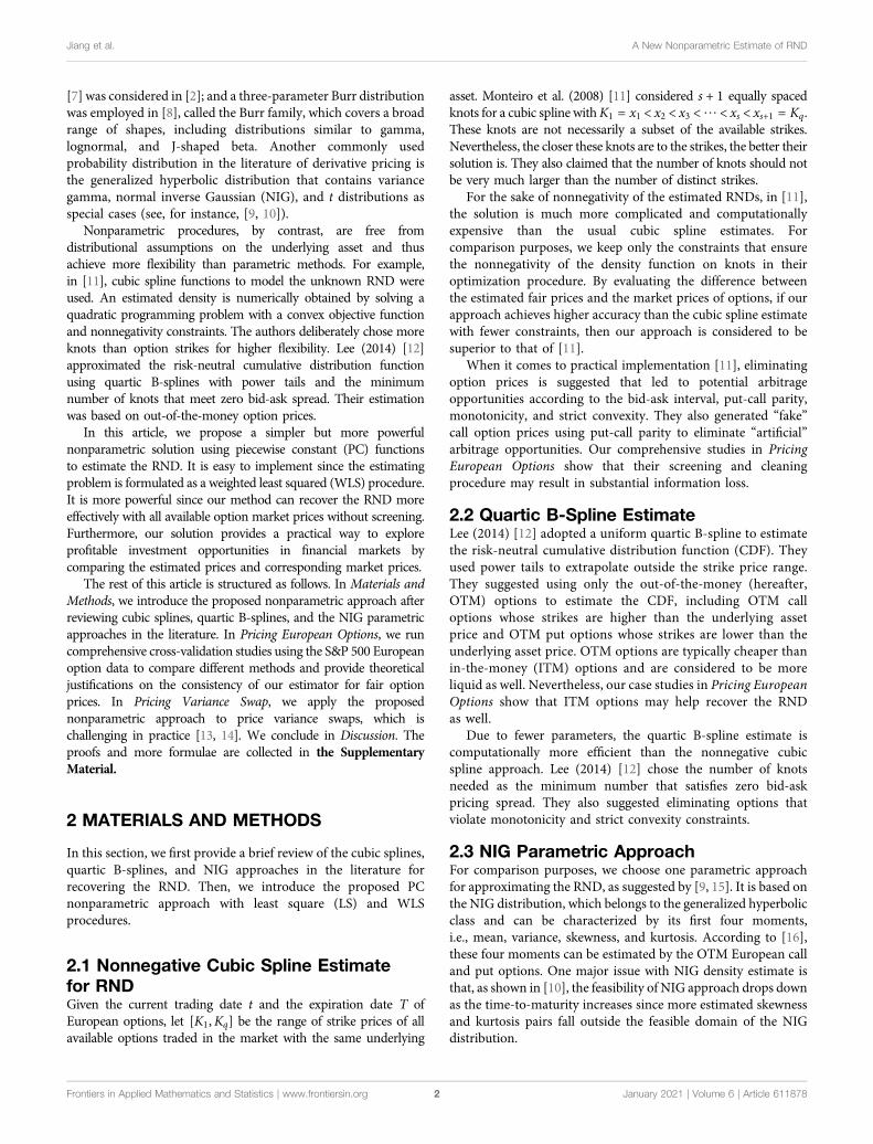
3. True: Realized price of a variance swap at expiration day Twithknown S0, S1, . . . , ST

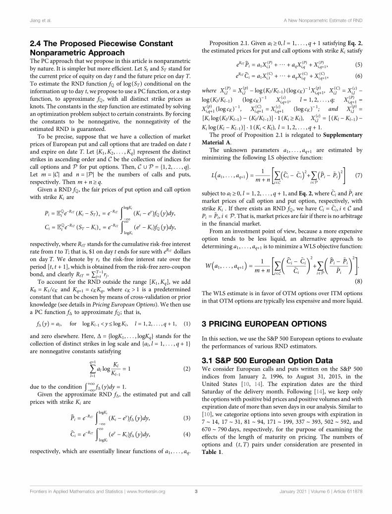
We present three ratios, OP/True, VF/True, and OP/VF, inFigures 2–4, respectively, against the remaining calendar daysof variance swaps. Compared with ‘True’ prices based onrealized underlying asset prices, Figure 2 and Figure 3suggest that OP and VF have a similar increasing patternalong with the remaining calendar days. This is in part due tothe uncertainty in the estimate of the variance, which increases

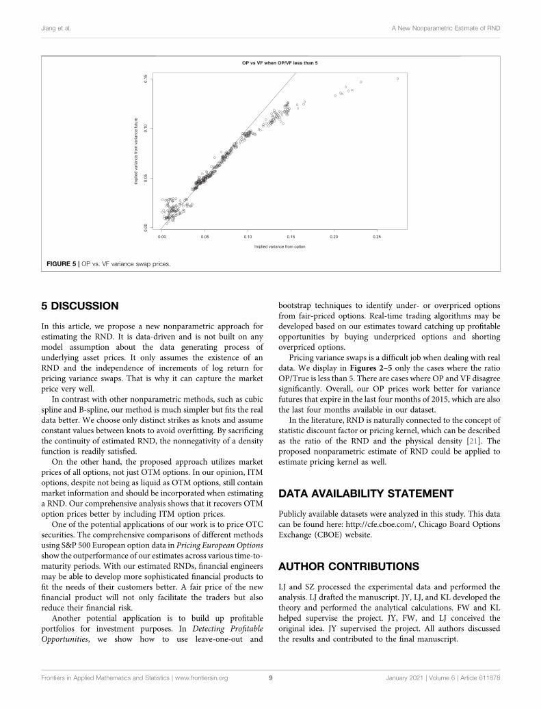
with the number of days to expiration. On the other hand,Figure 4 and Figure 5 show that the fair price OP based on ourproposed method matches the market price VF pretty well onvariance swaps with expiration between 365 and 800 days. Forvariance swaps expiring in less than 365 days (not shown here),OP and VF do not match well. This is plausibly attributed tothe fact that long-term options are more reasonable and stable,which are less likely to be affected by external factors or noises.For variance swaps longer than 800 days, the relatively low VFmight indicate underpriced variance futures.

FIGURE 3 | Ratio of VF/True variance swap prices vs. days to expiration.

FIGURE 4 | Ratio of OP/VF variance swap prices vs. days to expiration.

Frontiers in Applied Mathematics and Statistics | www.frontiersin.org January 2021 | Volume 6 | Article 6118788

Jiang et al. A New Nonparametric Estimate of RND

5 DISCUSSION

In this article, we propose a new nonparametric approach forestimating the RND. It is data-driven and is not built on anymodel assumption about the data generating process ofunderlying asset prices. It only assumes the existence of anRND and the independence of increments of log return forpricing variance swaps. That is why it can capture the marketprice very well.

In contrast with other nonparametric methods, such as cubicspline and B-spline, our method is much simpler but fits the realdata better. We choose only distinct strikes as knots and assumeconstant values between knots to avoid overfitting. By sacrificingthe continuity of estimated RND, the nonnegativity of a densityfunction is readily satisfied.

On the other hand, the proposed approach utilizes marketprices of all options, not just OTM options. In our opinion, ITMoptions, despite not being as liquid as OTM options, still containmarket information and should be incorporated when estimatinga RND. Our comprehensive analysis shows that it recovers OTMoption prices better by including ITM option prices.

One of the potential applications of our work is to price OTCsecurities. The comprehensive comparisons of different methodsusing S&P 500 European option data in Pricing European Optionsshow the outperformance of our estimates across various time-to-maturity periods. With our estimated RNDs, financial engineersmay be able to develop more sophisticated financial products tofit the needs of their customers better. A fair price of the newfinancial product will not only facilitate the traders but alsoreduce their financial risk.

Another potential application is to build up profitableportfolios for investment purposes. In Detecting ProfitableOpportunities, we show how to use leave-one-out and

bootstrap techniques to identify under- or overpriced optionsfrom fair-priced options. Real-time trading algorithms may bedeveloped based on our estimates toward catching up profitableopportunities by buying underpriced options and shortingoverpriced options.

Pricing variance swaps is a difficult job when dealing with realdata. We display in Figures 2–5 only the cases where the ratioOP/True is less than 5. There are cases where OP and VF disagreesignificantly. Overall, our OP prices work better for variancefutures that expire in the last four months of 2015, which are alsothe last four months available in our dataset.

In the literature, RND is naturally connected to the concept ofstatistic discount factor or pricing kernel, which can be describedas the ratio of the RND and the physical density [21]. Theproposed nonparametric estimate of RND could be applied toestimate pricing kernel as well.

DATA AVAILABILITY STATEMENT

Publicly available datasets were analyzed in this study. This datacan be found here: http://cfe.cboe.com/, Chicago Board OptionsExchange (CBOE) website.

AUTHOR CONTRIBUTIONS

LJ and SZ processed the experimental data and performed theanalysis. LJ drafted the manuscript. JY, LJ, and KL developed thetheory and performed the analytical calculations. FW and KLhelped supervise the project. JY, FW, and LJ conceived theoriginal idea. JY supervised the project. All authors discussedthe results and contributed to the final manuscript.

FIGURE 5 | OP vs. VF variance swap prices.

Frontiers in Applied Mathematics and Statistics | www.frontiersin.org January 2021 | Volume 6 | Article 6118789

Jiang et al. A New Nonparametric Estimate of RND

ACKNOWLEDGMENTS

We thank Liming Feng from the University of Illinois at Urbana-Champaign and Yuhang Liang from Northwestern University fortheir enormous help during data collection.

SUPPLEMENTARY MATERIAL

The SupplementaryMaterial for this article can be found online at:https://www.frontiersin.org/articles/10.3389/fams.2020.611878/full#supplementary-material.

REFERENCES

1. Malz AM. A simple and reliable way to compute option-based risk-neutraldistributions. In: Staff reportNew York, NY: Federal Reserve Bank of New York.(2014) p 677.

2. Melick W, Thomas C. Recovering an asset’s implied pdf from option prices: anapplication to crude oil during the gulf crisis. J Financ Quant Anal (1997) 32:91–115. doi:10.2307/2331318

3. Taboga M. Option-implied probability distributions: how reliable? How jagged?Int Rev Econ Finance (2016) 45:453–69. doi:10.1016/j.iref.2016.07.013

4. Breeden D, Litzenberger R. Prices of state-contingent claims implicit in optionprices. J Bus (1978) 51:621–51.

5. Bliss R, Panigirtzoglou N. Testing the stability of implied probability densityfunctions. J Bank Finance (2002) 26:381–422. doi:10.2139/ssrn.209650

6. Jarrow R, Rudd A. Approximate option valuation for arbitrary stochasticprocess. J Financ Econ (1982) 10:347–69. doi:10.1016/0304-405X(82)90007-1

7. Ritchey R. Call option valuation for discrete normal mixtures. J Financ Res(1990) 13:285–96. doi:10.1111/j.1475-6803.1990.tb00633.x

8. Sherrick B, Irwin S, Forster D. Option-based evidence of the nonstationarity ofexpected SP 500 futures price distributions. J Futures Mark (1992) 12:275–90.doi:10.1002/fut.3990120304

9. Eriksson A, Ghysels E, Wang F. The normal inverse Gaussian distribution andthe pricing of derivatives. J Deriv (2009) 16:23–37. doi:10.3905/JOD.2009.16.3.023

10. Ghysels E, Wang F. Moment-implied densities: properties and applications.J Bus Econ Stat (2014) 32:88–111. doi:10.1080/07350015.2013.847842

11. Monteiro A, Tutuncu R, Vicente L. Recovering risk-neutral probability densityfunctions from options prices using cubic splines. Eur J Oper Res (2008) 187:525–42. doi:10.1016/j.ejor.2007.02.041

12. Lee S. Estimation of risk-neutral measures using quartic b-spline cumulativedistribution functions with power tails. Quant Finance (2014) 14:1857–79.doi:10.1080/14697688.2012.742202

13. Zhu SP, Lian GH. A closed-form exact solution for pricing variance swaps withstochastic volatility.Math Finance (2010) 21:233–56. doi:10.1111/j.1467-9965.2010.00436.x

14. Carr P, Lee R, Wu L. Variance swaps on time-changed Lévy processes. FinanceStochast (2012) 16:335–55. doi:10.1007/s00780-011-0157-9

15. Eriksson A, Ghysels E, Forsberg L. Approximating the probability distributionof functions of random variables: a new approach. Montreal, Canada:Cirano(2004) p 503.

16. Bakshi G, Kapadia N, Madan D. Stock return characteristics, skew laws, andthe differential pricing of individual equity options. Rev Financ Stud (2003) 16:101–43. doi:10.2139/srn.282451

17. Han Y, Zhao L. A closed-form pricing formula for variance swaps under MRG-Vasicek model. Comput Appl Math (2019) 38:142. doi:10.1007/s40314-019-0905-6

18. Liu W, Zhu SP. Pricing variance swaps under the Hawkes jump-diffusionprocess. J Futures Mark (2019) 39:635–55. doi:10.1002/fut.21997

19. Rompolis LS, Tzavalis E. Retrieving risk neutral moments and expectedquadratic variation from option prices. Rev Quant Finance Account (2017)48:955–1002. doi:10.2139/ssrn.936670

20. Biscamp L, Weithers T. Variance swaps and cboe s and p 500 variance futures.Chicago Trading Company, LLC. (2007) p 25.

21. Beare BK, Schmidt LD. An empirical test of pricing kernel monotonicity. J ApplEconom (2016) 31:338–56. doi:10.1002/jae.2422

Conflict of Interest: The authors declare that the research was conducted in theabsence of any commercial or financial relationships that could be construed as apotential conflict of interest.

Copyright © 2021 Jiang, Zhou, Li, Wang and Yang. This is an open-access articledistributed under the terms of the Creative Commons Attribution License (CC BY).The use, distribution or reproduction in other forums is permitted, provided theoriginal author(s) and the copyright owner(s) are credited and that the originalpublication in this journal is cited, in accordance with accepted academic practice. Nouse, distribution or reproduction is permitted which does not comply with these terms.

Frontiers in Applied Mathematics and Statistics | www.frontiersin.org January 2021 | Volume 6 | Article 61187810

Jiang et al. A New Nonparametric Estimate of RND

Supplementary MaterialforA New Nonparametric Estimate of the Risk-NeutralDensity with Applications to Variance Swaps

A. PROOF OF PROPOSITION 2.1We rewrite the call and put option prices in Eqs 3, 4 in terms of a1, a2, . . . , aq, aq+1 as follows

eRtT Pi =

∫ logKi

−∞(Ki − ey)f∆(y)dy

=

q+1∑l=1

∫ logKl

logKl−1

(Ki − ey)aldy · 1(Ki ≥ Kl)

=

q+1∑l=1

al[(Ki logKl

Kl−1)− (Kl −Kl−1)] · 1(Ki ≥ Kl), i ∈ P

(S1)

eRtT Ci =

∫ ∞logKi

(ey −Ki)f∆(y)dy

=

q+1∑l=1

∫ logKl

logKl−1

(ey −Ki)aldy · 1(Ki ≤ Kl−1)

=

q+1∑l=1

al[(Kl −Kl−1)−Ki logKl

Kl−1] · 1(Ki < Kl), i ∈ C

(S2)

Let X(p)i,l = [Ki log(Kl/Kl−1)− (Kl −Kl−1)] · 1(Ki ≥ Kl), l = 1, 2, . . . , q + 1 be an entry of the design

matrix for put options; and X(c)i,l = [(Kl −Kl−1)−Ki log(Kl/Kl−1)] · 1(Ki < Kl), l = 1, 2, . . . , q + 1

for call options. From Eq. 2, aq+1 can be represented by a1, a2, . . . , aq, as

aq+1 =

(1−

q∑l=1

al logKl

Kl−1

)(log cK)−1 (S3)

1

Supplementary Material

Plugging Eq. S3 into Eqs S1, S2, we obtain

eRtT Pi =

q+1∑l=1

alX(p)i,l

= a1X(p)i,1 + a2X

(p)i,2 + · · ·+ aqX

(p)i,q

+

(1− a1 log

K1

K0− · · · − aq log

Kq

Kq−1

)(log cK)−1X

(p)i,q+1

= a1[X(p)i,1 − (log

K1

K0)(log cK)−1X

(p)i,q+1] + · · ·

+ aq[X(p)i,q − (log

Kq

Kq−1)(log cK)−1X

(p)i,q+1] +

1

log cKX

(p)i,q+1

4= a1X

(P )i,1 + a2X

(P )i,2 + · · ·+ aqX

(P )i,q +X

(P )i,q+1, i ∈ P

(S4)

where X(P )i,l = X

(p)i,l − (logKl/Kl−1)(log cK)−1X

(p)i,q+1, l = 1, 2, . . . , q and X(P )

i,q+1 = X(p)i,q+1/ log cK .

Similarly for call options,

eRtT Ci =

q+1∑l=1

alX(c)i,l

= a1X(c)i,1 + a2X

(c)i,2 + · · ·+ aqX

(c)i,q

+

(1− a1 log

K1

K0− · · · − aq log

Kq

Kq−1

)(log cK)−1X

(c)i,q+1

= a1[X(c)i,1 − (log

K1

K0)(log cK)−1X

(c)i,q+1] + · · ·

+ aq[X(c)i,q − (log

Kq

Kq−1)(log cK)−1X

(c)i,q+1] +

1

log cKX

(c)i,q+1

4= a1X

(C)i,1 + a2X

(C)i,2 + · · ·+ aqX

(C)i,q +X

(C)i,q+1, i ∈ C

(S5)

where X(C)i,l = X

(c)i,l − (logKl/Kl−1)(log cK)−1X

(c)i,q+1, l = 1, . . . , q and X(C)

i,q+1 = X(c)i,q+1/ log cK . �

B. PROOF OF THEOREM 3.1Given ε > 0, let δ1 =

√εeRtT /[3(1 + cK + e)] > 0. There exists −∞ < A < 0 < B <∞, such that,∫ A

−∞fQ(x)dx < δ1,

∫ A

−∞exfQ(x)dx < δ1,

∫ ∞B

fQ(x)dx < δ1,

∫ ∞B

exfQ(x)dx < δ1

Let δ2 =√εeRtT−B−1/[3(B − A + 2)] > 0. Since fQ is continuous, there exists a δ > 0, such that, for

any x1, x2 ∈ [A− 1, B + 1],|fQ(x1)− fQ(x2)| < δ2

as long as |x1 − x2| < δ.

2

Supplementary Material

For small enough K1, |∆| and large enough q,Kq, there exist integers u, v, such that, 1 < u < u+ 1 <v < v + 1 < q, logKu ≤ A < logKu+1, logKv < B ≤ logKv+1, |∆| < δ.

We construct a f∆ by defining

a1 = (log cK)−1

∫ logK1

−∞fQ(x)dx ≥ 0

ai = [log(Ki/Ki−1)]−1

∫ logKi

logKi−1

fQ(x)dx ≥ 0, i = 2, . . . , q

aq+1 = (log cK)−1

∫ ∞logKq

fQ(x)dx ≥ 0

It can be verified that∫∞−∞ f∆(x)dx =

∑q+1i=1 ai log(Ki/Ki−1) = 1. Let

∆f = maxu≤i≤v

(max

logKi≤x≤logKi+1

fQ(x)− minlogKi≤x≤logKi+1

fQ(x)

)Then |∆| < δ implies ∆f ≤ δ2. It can be verified that

|Ci − Ci| <

√ε/3, for i = v + 1, . . . , q

2√ε/3, for i = u, . . . , v√ε, for i = 1, . . . , u− 1

|Pi − Pi| <

√ε/3, for i = 1, . . . , u

2√ε/3, for i = u+ 1, . . . , v + 1√ε, for i = v + 2, . . . , q

In other words, there exist a1, . . . , aq+1, such that, (Ci − Ci)2 < ε, (Pi − Pi)

2 < ε, for i = 1, . . . , q. Itimplies the (a1, . . . , aq+1) that minimizes L(a1, . . . , aq+1) also satisfies

1

2q

[q∑

i=1

(Ci − Ci)2 +

q∑i=1

(Pi − Pi)2

]< ε

which leads to the conclusion. �

Frontiers 3

Supplementary Material

C. PROOF OF PROPOSITION 4.1Since EQ

t [∑T

i=1R2i ] =

∑ti=1R

2i +

∑Ti=t+1 E

Qt [R2

i ], the key part

T∑i=t+1

EQt [R2

i ] =T∑

i=t+1

EQt [log

SiSi−1

]2

=T∑

i=t+1

[EQt (logSi)

2 + EQt (logSi−1)2 − 2EQ

t (logSi)(logSi−1)]

=T∑

i=t+1

EQt (logSi)

2 +T∑

i=t+1

EQt (logSi−1)2 − 2

T∑i=t+1

EQt [logSi−1 + log(

SiSi−1

)][logSi−1]

=T∑

i=t+1

EQt (logSi)

2 +T∑

i=t+1

EQt (logSi−1)2 − 2

T∑i=t+1

EQt (logSi−1)2

− 2T∑

i=t+1

EQt [logSi−1][log(

SiSi−1

)]

= EQt [logST ]2 − [logSt]

2 − 2T∑

i=t+1

EQt [logSi−1][log(

SiSi−1

)]

= EQt [logST ]2 − [logSt]

2 − 2T∑

i=t+1

EQt [logSi−1]EQ

t [log(SiSi−1

)]

= EQt [logST ]2 − [logSt]

2 − 2T∑

i=t+1

[EQt logSi−1EQ

t logSi − (EQt logSi−1)2]

Then Eq. 12 can be obtained by plugging EQt [∑T

i=1R2i ] into Eq. 11. �

D. LINEAR INTERPOLATION FOR 1ST AND 2ND MOMENTS IN SECTION 4.1Mean imputation Suppose the trading day is t and the expiration day is T . We denote all possibleexpiration dates of traded contracts by t+ n1, t+ n2, . . . . Suppose the time point to be imputed is t+ n0.Given all the information available at day t, logSt can be regarded as its expectation at day t, EQ

t logSt.Therefore, we consider cases separately according to whether or not t+ n0 is in the interval [t, t+ n1] andthen apply linear interpolation to obtain the mean of logSt+n0 . More specifically, there are two cases:

Case 1: n0 ∈ [0, n1] and EQt (logSt+n1) has been calculated.

EQt (logSt+n0) = EQ

t (logSt+n1)− (n1 − n0)[EQt (logSt+n1)− logSt]

n1

=n0EQ

t (logSt+n1) + (n1 − n0) log(St)

n1

4

Supplementary Material

Case 2: n0 ∈ [ni, ni+1] for some i = 1, 2, . . .. The expectations EQt (logSt+ni) and EQ

t (logSt+ni+1)have already been calculated.

EQt (logSt+n0) =

(n0 − ni)[EQt (logSt+ni+1)− EQ

t (logSt+ni)]

ni+1 − ni+ EQ

t (logSt+ni)

=(n0 − ni)EQ

t (logSt+ni+1) + (ni+1 − n0)EQt (logSt+ni)

ni+1 − ni

Variance Imputation In order to calculate the variance VQt (logSt+n0) at day t, we use a similar

interpolation based on the available variances of log returns at day t with expiration T . Based on thescatterplot (not shown here) of all available variances that we have from the existing contracts, the trend ofvariances has a curved pattern against the number of days to expiration. More specifically, it is roughly aquadratic curve. Before we implement a linear interpolation, we first perform a square-root transformationof variances.

Case 1: n0 ∈ [0, n1]. VQt (logSt+n1) has been calculated. Then

√VQt (logSt+n0) =

n0

√VQt (logSt+n1)

n1

Case 2: n0 ∈ [ni, ni+1] for some i = 1, 2, . . .. The values VQt (logSt+ni) and VQ

t (logSt+ni+1) havebeen calculated. Then√

VQt (logSt+n0)

=

√VQt (logSt+n0)−

√VQt (logSt+ni) +

√VQt (logSt+ni)

=

(n0 − ni)[√

VQt (logSt+ni+1)−

√VQt (logSt+ni)

]ni+1 − ni

+

√VQt (logSt+ni)

=(n0 − ni)

√VQt (logSt+ni+1) + (ni+1 − n0)

√VQt (logSt+ni)

ni+1 − ni.

Then the second moment is

EQt (logSt+n0)2 = [EQ

t (logSt+n0)]2 + VQt (logSt+n0)

A fair price of variance swap V St,T can be obtained by the pricing formula Eq. 11.

Frontiers 5