a new motion management method for lung tumor … · a new motion management method for lung tumor...

A New Motion Management Methodfor Lung Tumor Tracking Radiation Therapy

NORIYASU HOMMATohoku University

Cyberscience Center6-6-05 Aoba, Aoba-ku

Sendai 980-8579JAPAN

[email protected]

MASAO SAKAITohoku University

Center Inform. Tech. Edu.41 Kawauchi, Aoba-ku


[email protected]

HARUNA ENDOTohoku University

Graduate School of Medicine2-1 Seiryo-machi, Aoba-ku


[email protected]

MASATOSHI MITSUYATohoku University



[email protected]

YOSHIHIRO TAKAITohoku University



[email protected]

MAKOTO YOSHIZAWATohoku University

Cyberscience Center6-6-05 Aoba, Aoba-ku


[email protected]

Abstract: We propose a new motion management method for lung tumor tracking radiotherapy by using a noveltime series prediction technique. In radiotherapy, the target motion often affects the conformability of the therapeu-tic dose distribution delivered to thoracic and abdominal tumors, and thus tumor motion monitoring systems havebeen developed. Even we can observe tumor motion accurately, however, radiotherapy systems may inherentlyhave mechanical and computational delays to be compensated for synchronizing dose delivery with the motion.For solving the delay problem, we develop a novel system to predict complex time series of the lung tumor motion.An essential core of the system is an adaptive prediction modeling with a phase locking technique by which time-varying cyclic dynamics is transferred into a time invariant one. Simulation studies demonstrate that the proposedsystem can achieve a clinically useful high accuracy and long-term prediction of the average error1.05 ± 0.99[mm] at1 [sec] ahead prediction.

Key–Words:Time series prediction, adaptive modeling, radiation therapy, lung tumor, and motion management.

1 Introduction

It is important for radiation therapy to give sufficientdose to tumor and to reduce normal tissue toxicity. Byusing image-guided techniques, extracranial stereo-tactic radiotherapy (ESRT) can achieve a precise dosedelivery in a short time [1] and thus have a goodoutcome that is comparable to the performance ofsurgery [2]. In addition to this, delivering a highlyconformal dose distribution to a “static” tumor targetin three-dimensional space is largely solved by tech-niques such as intensity modulated radiation therapy(IMRT) [3, 4].

In radiation therapy, it is known that the targetmotion often affects the conformability of the thera-peutic dose distribution delivered to thoracic and ab-dominal tumors. Tumor motions can not only be asso-ciate with patient’s stochastic movements and system-atic drifts, but also involve internal movements causedby such as respiration and cardiac cycles [5].

To take into account such “dynamic” nature ofthe internal organ motion during the course of radia-

tion therapy, several techniques have been proposedand evaluated in clinical use. A simple method is toincrease the planning target volume (PTV) to coverthe possible range of motion of the target [6], but un-desirably it results in an increased dose to the nor-mal tissues surrounding the tumor. One of the othermethods to treat the respiratory motion of the lungtumor is a breath-hold technique [7]. Since the respi-ration may be dominant over the lung tumor motion,the tumor can be regarded as a static target by usingsuch technique to stop the respiration. Geometric gat-ing method is also this kind of techniques to limit themotion effect [8, 9, 10, 11]. They are, however, notdesirable techniques because of patient interventionby the breath-hold or beam interruption by the gating.In this sense, tumor tracking by moving the radiationsource [12, 13, 14] or the beam defined by multileafcollimator [15, 16, 17] can be in an ideal direction.

To achieve such tumor tracking, several methodshave been proposed. Among these, direct measure-ments of a fiducial gold marker of the tumor posi-tion by fluoroscopy imaging techniques [18, 19, 20,

WSEAS TRANSACTIONS on SYSTEMSNoriyasu Homma, Masao Sakai, Haruna Endo, Masatoshi Mitsuya, Yoshihiro Takai, Makoto Yoshizawa

ISSN: 1109-2777 471 Issue 4, Volume 8, April 2009

Figure 1:An example of X-ray images of the fiducial gold marker implanted into a lung tumor. Three-dimensionalcoordinates of the tumor motion can be measured by using the marker’s position.

21, 22], as shown in Fig. 1 for example, are morepromising than indirect ones such as external skinmarker tracking [11, 23, 24] and breath monitoringtechniques [25]. Such tracking systems may involvemechanical and computational delays to control themultileaf collimator and for image and time seriesprocessings of the tumor motion. Thus, the time delaymust be compensated by predicting the tumor motionto accomplish a real-time tracking [5]. The desiredaccuracy of the tumor location can be within about1 [mm] at up to 1 [sec] ahead prediction. This is ahighly accurate condition for the complex dynamicsof the tumor motion.

In this paper, we propose a new system realizingsuch highly accurate prediction of lung tumor motionfor tracking radiation therapy. The proposed systemtakes into account the complex dynamics by using anadaptive modeling for the prediction.

The rest of this paper consists of as follows. Wewill investigate nature of the motion first, by usingtime series analysis techniques in section 2. Thenprediction method will be developed in section 3 byusing results of the analysis. In section 4, predic-tion accuracy of the proposed system will be evalu-ated by using real data of tumor motions in whichthe performances of the prediction systems consist-ing of a smoothing prediction model designed byHolt-Winters seasonal (HWS) method [26] and moregeneral seasonal ARIMA (SARIMA) model [27] arecompared to a conventional prediction method. Con-

cluding remarks will be given in section 5.

2 Motion of Lung Tumor

Three-dimensional time series of human lung tumormotion was observed at Hokkaido University Hospi-tal [28]. An example of the tumor location at superiorsegment of right lung, S6, is shown in Fig. 2. A domi-nant source of the tumor motion is respiration, but theothers such as caused by cardiac motion may also beincluded in the time series.

Figure 2:Structure of a human lung.



t

y1(t)

y2 y3

y1

y2(t)

y3(t)

Figure 3: Preprocessed time seriesy(t) of the ob-served tumor marker motion at S6 of the lung.

2.1 Preprocessing (noise reduction) of thetime series

A fiducial gold marker implanted into the lung tu-mor was used to measure the three-dimensional co-ordinates of the tumor motion. The spatial resolutionand sampling period were 0.01[mm] and 0.033[sec](30[Hz]), respectively. To reduce observational noiseand avoid abnormal data involved in raw data of thetime series, we preprocessed the time series by usingseveral filters such as the Kalman filter [29] and sta-tistical filters. An example of the preprocessed timeseries

y(t) = [y1(t) y2(t) y3(t)] (1)

t = 1, 2, . . . , 5000, are shown in Fig. 3. Here el-ements of vectory(t) at time t [step], y1(t), y2(t),andy3(t) [mm], are the marker’s position of the lat-eral, cephalocaudal, and anteroposterior directions,respectively. Note that the time series of the vectory(t), t = 1, 2, ..., can be obtained in real-time.

For the teaching data of time series prediction,we further reduced the observational impulse noiseinvolved in the time seriesy(t), t = 1, 2, ..., inEq. (1) by using statistical filters, and then reducedhigh frequency noise by using a low pass filter thatdeletes unnecessary high frequency components thatare higher than0.1 × fmax [Hz]. Here fmax is themaximum frequency of the digital Fourier transformspectrum under the sampling period. The statisticscan be computed by using all data of the time seriesfor t = 1, 2, . . . , 5000 in Fig. 3. The noise reducedtime seriesy∗(t) = [y∗1(t) y∗2(t) y∗3(t)] are shown inFig. 4 and assumed as the real motion of the fiducial

t

y*1 (t)

y*2 y*3

y*1

y*2 (t)

y*3 (t)

Figure 4:The noise reduced time seriesy∗(t) of themarker motion.

marker of the tumor.

2.2 Cyclic dynamics

There can be cyclic dynamics with approximately90[steps] periods of respiratory motion involved in thefiducial marker motion of the lung tumor as seen inFigs. 3 and 4. Note that the periods of the cycliccomponents and rhythmic dynamics can be fluctuatedwhen the respiratory dynamics are changed. If pa-tients are in rest, however, respiratory dynamics is al-most cyclic and thus the dominant dynamics of timeseries is also cyclic as seen in Fig. 3.

We calculate the autocorrelation function (ACF),γ, of the time series for further analysis of the cyclicdynamics involved in the tumor motion. Fig. 5 showsγ(t, k) of a sample time series in the cephalocau-dal direction,[y∗2(t − 150) y∗2(t − 149) · · · y∗2(t +149) y∗2(t+150)], within a time window (301 steps) as

ç(t; k)

Figure 5:Autocorrelation function,γ(t, k), of y∗2.



t t t

k k k

ç1(t; k) ç2(t; k) ç3(t; k)

Figure 6:Autocorrelation functions ofY (t).

t

s i(t;1)

s1(t; 1) s2(t; 1) s3(t; 1)

Figure 7: Periodssi, i = 1, 2, 3, of Y (t) as func-tions of timet. It can be seen that periods are slightlyfluctuated aroundsi = 90.

a function of timet [step] and the shiftk [step]. Notethat the first peak of the ACF at a shiftk(≥ 1) corre-sponds to the dominant period of the cyclic dynamics.Then from the autocorrelation function analysis, it isrevealed that the dominant periods are approximately90 [steps] as expected above. Furthermore, the peri-ods are slightly and smoothly fluctuated and thus theycan be time variant. As shown in Figs. 6 and 7, ACFsfor time series of the other two directions,y∗1 andy∗3,are almost similar to that ofy∗2.

In the following section, we will build a modelwith time variant periods for predicting such fluctu-ated motion of the lung tumor.

3 Prediction Method

3.1 Concept of prediction algorithm

Fig. 8 shows a tumor motion prediction system pro-posed in this paper. Let us predict theh-step (h ≥ 1)ahead fiducial marker’s position of the lung tumor.

*

Figure 8:The proposed prediction system.

The predicted positiony∗(t + h) of the actual (noisereduced) tumor positiony∗(t+h) is calculated by us-ing the real-time preprocessed time series available attime t

Y (t) = [y(1) y(2) · · ·y(t − 1) y(t)]T (2)

Basic ideas of the prediction algorithm are as fol-lows. As analyzed in section 2.2, the target time se-riesy∗(t) may include a complex dynamics with timevariant periods. Thus, far past information involvedin the whole time seriesY (t) is less important oreven can have a bad effect on the prediction accu-racy. Then, the prediction model can be built based onthe not far past information of the time series. Notethat the current period is one of the most importantpiece of information for the prediction because thecyclic dynamics makes the prediction be precise. Inthis sense, the proposed algorithm tries to estimate thecurrent dominant period as precise as possible by us-ing a flesh piece of information involved in the currenttime series available.

Let us consider the current period vectors∗(t) =[s∗1(t) s∗2(t) s∗3(t)] of the time seriesy∗(t) =[y∗1(t) y∗2(t) y∗3(t)] at timet, and denote its estimationass(t) = [s1(t) s2(t) s3(t)]. The estimation of thes∗can be calculated by using the autocorrelation func-tion analysis of a flesh sample time series with a timelengthL given asyi(τ), τ = t − L, t − L + 1, . . . , t,available at timet. To use the important piece of in-formation included in the flesh sample of the time se-ries,L can cover time series for more than the currentperiod in time length,si(t−1) < L, but should not betoo large as mentioned above. Here if the estimatedperiod is changed,si(t−1) = si(t), then the model ofcyclic dynamics is adapted to the new current periodsi(t). The finalh-step ahead predictiony∗(t+h) canbe calculated based on the adapted model of the newcyclic dynamicsY (t) as shown in Fig. 8.

3.2 Prediction model

As prediction models of the lung tumor motion thatis mainly caused by the respiration with time variantcyclic periods, we adopt two models of the time serieshere. One is Holt-Winters exponential smoothing, asmoothing model designed by the HWS method, andthe other is a seasonal ARIMA (SARIMA) model.Note that, however, any other linear or nonlinearmodels including neural networks can be incorpo-rated into the proposed adaptive prediction method.

3.2.1 Holt-Winters exponential smoothing

The HWS method can provide an easy design of theseasonal model to predict1-step ahead of the time



series ifthe period of cyclic dynamics is known andtime invariant. The general formulations of the HWSis given as follows.

y∗i (t + h) = ai(t) + bi(t)h+ci(t − si(t) + mod (h, si(t))) (3)

ai(t) = α (yi(t) − ci(t))+(1 − α) (ai(t − 1) + bi(t)) (4)

bi(t) = β (ai(t) − ai(t − 1))+(1 − β) (bi(t − 1)) (5)

ci(t) = γ (yi(t) − ai(t))+(1 − γ) (ci(t − si(t))) (6)

where the initial values at timet0(> si(t0)) can beinitialized by

ai(t0) = yi(t0) (7)

bi(t0) =yi(t0) − yi(t0 − si(t0) + 1)

si(t0)(8)

ci(t0 − k) = yi(t0 − k) − (yi(t0 − si(t0) + 1)+ (si(t0) − k) · bi(t0))· · · k = 0, 1, 2, · · · , si(t0) (9)

In such case, only three smoothing parameters,implying the ratio of use the predicted data to the pre-vious actual data for smoothing, may be designed asvalues between 0 and 1; 0 implies smoothing by onlythe actual data, while 1 implies smoothing by only thepredicted data. The three parameters,0 ≤ α, β, γ ≤1, are ratios for smooth calculation of the trend level,the gradient of trend, and cyclic component, respec-tively.

On the other hand, the easy design restricts free-dom of the model and thus the prediction accuracy islimited in the case of complicated time series. Also,modeling errors may be accumulated for a mid- orlong-term prediction(h ≫ 1) and the prediction willresult in failure with a large error beyond the toler-ance.

3.2.2 Seasonal ARIMA model

The other model, the general SARIMA model of thetime series,[x(0) x(1) · · · x(t)], with periods [steps]of cyclic dynamics can be given as follows.

φ(B)Φ(Bs)(1 − B)d(1 − Bs)Dx(t) = θ(B)Θ(Bs)e(t)

(10)

φ(z) = 1 − φ1z − φ2z2 − · · · − φpz

p (11)

Φ(z) = 1 − Φ1z − φ2z2 − · · · − φP zP (12)

θ(z) = 1 + θ1z + θ2z2 + · · · + θqz

q (13)

Θ(z) = 1 + Θ1z + Θ2z2 + · · · + ΘQzQ (14)

wheree(t) is the Gaussian noise of which average andvariance are0 andσ2, respectively.B is a time delayoperator defined as

Bkx(t) = x(t − k)

The parametersd, D, p, P , q, andQ representdimensions of corresponding terms, respectively. Be-cause of high degree of design parameter freedom ofthe SARIMA model, the model can predict compli-cated dynamics with a high precision. It is often,however, hard to design such appropriate parametersof the model for the precise prediction.

To design the SARIMA model, we first make acompensated time seriesx(t) from the adapted pre-processed time seriesy(t) as

x(t) = y(t) − z(t) (15)

wherez(t) = [z1(t) z2(t) z3(t)] is a trend level vectorat timet of the time seriesy(t) defined by

zi(t) =1

si(t)

t∑τ=t−si(t)+1

yi(τ) (16)

i = 1, 2, 3. Then, the SARIMA model can be build byusing the compensated time series with a time lengthof L given as

X(t) = [x(t − L) x(t − L + 1) · · · x(t)]T (17)

For avoiding the accumulation of the modeling errorat each step, we directly design anh-step ahead pre-diction model instead of repeatedly use of the 1-stepahead prediction one. To this end, the following con-straint can be introduced.

φi = 0 · · · if mod(i, [h/2]) = 0 (18)

where [x] denotes an operator that gives maximuminteger not greater thanx and mod(i, k) gives the re-mainder on division ofi by k.

4 Results and Discussions

4.1 Adaptive compensation

The estimation of the current dominant periods ofcyclic dynamics was conducted during prediction forthe model adaptation. The estimation results areshown in Figs. 9 and 10. As seen in these figure, esti-mated periods as functions of time converge in around90 after 600 steps. A reason why such long (600)steps were needed for convergence of the estimatedperiods may be due to the limitation of the changes ofthe estimated periods given as|si(t) − si(t − 1)| ≤1, i = 1, 2, 3, with the initial valuessi(0) = 1 to



t t t

k k k

ç1(t; k) ç2(t; k) ç3(t; k)

Figure 9: Autocorrelation functions of the compen-sated time seriesY (t).

t

s i(t;1)

s1(t; 1) s2(t; 1) s3(t; 1)

Figure 10:Periodssi, i = 1, 2, 3, of the compensatedtime seriesY (t) as functions of timet. Comparedto Figs. 6 and 7, the compensated periods are almostconstant after the convergence (t >600).

avoid undesirable oscillation of the estimation by rad-ical changes of the estimation. This may, however, re-quire only additional20 [sec] observations before theactual therapeutic irradiation in clinical use.

On the other hand, compared to Figs. 6 and 7,the periods of the compensated time series are al-most constant after the convergence. Fig. 11 showssuperimposition of the time series for each compen-sated period on the phase axis by using the periodestimated. Compared to the original time series, thephases (wave shapes) of the compensated time seriesfor different periods are synchronized with each other.As is clear from these figures, the proposed compen-sation is effective for the phase synchronization of thefluctuated time series.

4.2 Prediction results

We have tested the proposed system using a predic-tion task in which the preprocessed time seriesY (t)of fiducial marker’s motions of several lung tumorsare used. To evaluate the performance under the worst(longest-term) condition required in clinical use, themaximum length ofh = 30-step (1[sec]) ahead pre-diction was conducted first.

An example of the resulting time series fort =3000 to 5000 predicted by the smoothing model de-signed by the HWS method is shown in Fig. 12. Inthis result, the smoothing parameters were experi-mentally designed asα = 0.01, β = 0.05, andγ = 0.7, respectively.

On the other hand, for the same target time series,

the prediction result by the adaptive SARIMA modelis shown in Fig. 13. Here, the objective predictionstepsh = 30 is a mid- or long- term. In this case,to avoid the overfitting problem for the model design,we simplified the model asd = D = q = Q = 0,and experimentally designed as the rest of the dimen-sional parametersp = 5h andP = 6si(t), respec-tively. Referential time series predicted by the zero-order hold model given asy∗(t + h) = y(t) are alsoshown in Figs. 12 and 13. Note that the parameters ofboth models can be optimized by using some criteriasuch as Akaike’s Information Criterion (AIC) [30].

As is clear from these figures, it can be concludedthat prediction accuracy of both smoothing and adap-tive SARIMA models is superior to that of the zero-order hold model, and the SARIMA model is slightlyfurther superior to the smoothing model.

To further clarify the effect of the adaptation tothe fluctuated periods, we have compared the normalSARIMA and the adaptive SARIMA models. Forsimplicity, we changed only one parameterP and therest of the parameters wered = D = p = q = Q =0. Then,Φk = 1/P, k = 1, 2, · · · , P .

Table 1 summarizes prediction errors at 1 [sec]ahead by both SARIMA models with the parameterP = 1, 2, . . . , 5. First, the results show that the errorsby the adaptive SARIMA model is less than the nor-mal SARIMA model for all cases ofP = 2, 3, 4, 5. Inother words, the adaptive SARIMA is superior thanthe normal one. ForP = 1, there is no differencebetween the normal and adaptive SARIMA modelssince no compensation is conducted for the time se-ries for the current period.

Second,P = 2 is the optimal condition for1 ≤ P ≤ 5. This suggests that there is the opti-mal length of the time series including a useful pieceof information for the prediction. Less or more lengthof the time series can affect badly on the prediction er-ror as discussed in section 3.1. The conditionP = 2is generally a reasonable for SARIMA model [31].Thus, the comparison demonstrates the effect of real-

Table 1: The prediction errors (mean± SD) at 1 [sec](=30 steps) ahead by the normal SARIMA and adap-tive SARIMA with P = 1, 2, · · · , 5.

P Normal SARIMA Adaptive SARIMA

1 1.0954± 0.99842 1.0690± 0.9766 1.0497± 0.99473 1.2225± 1.1656 1.1175± 1.02424 1.4166± 1.3576 1.2201± 1.11665 1.6112± 1.4736 1.2884± 1.1954



P re d ic te d w a veC u rre n t w a ve

y1(t) y2(t) y3(t)

y1(t) y2(t) y3(t)

Figure 11:Superimposition of wave shapes of time series for each period. Upper and lower columns show waveshapes of the original time seriesY (t) and the compensated time seriesY (t), respectively. All the periods forY (t) were compensated tosi = 90 in this case. Red and purple lines indicate the wave shapes of the current andpredicted periods, respectively.

y1 (t+h)

y*1 (t)

(t)1

y2 (t+h)

y*2 (t)

(t)2

y3 (t+h)

y*3 (t)

(t)3

t

y (t+h)

y* (t)

(t)

i

i

i

y*~

y*~

y*1

*2

*3

~

y~ y~

y*~

y*~

Figure 12:Comparison of time series between the target (blue dotted lines) and the predictions (red lines) at 1[sec] (30 steps) ahead by the HWS model.



y1 (t+h)

(t)

(t)

y2 (t+h)

(t)

(t)

y3 (t+h)

(t)

(t)

y (t+h)

(t)

(t)

i

t

3

y*i

iy*~

y*1

1y*~

y*2

2y*~

y*3

3y*~

y*1~

*2y~ *y~

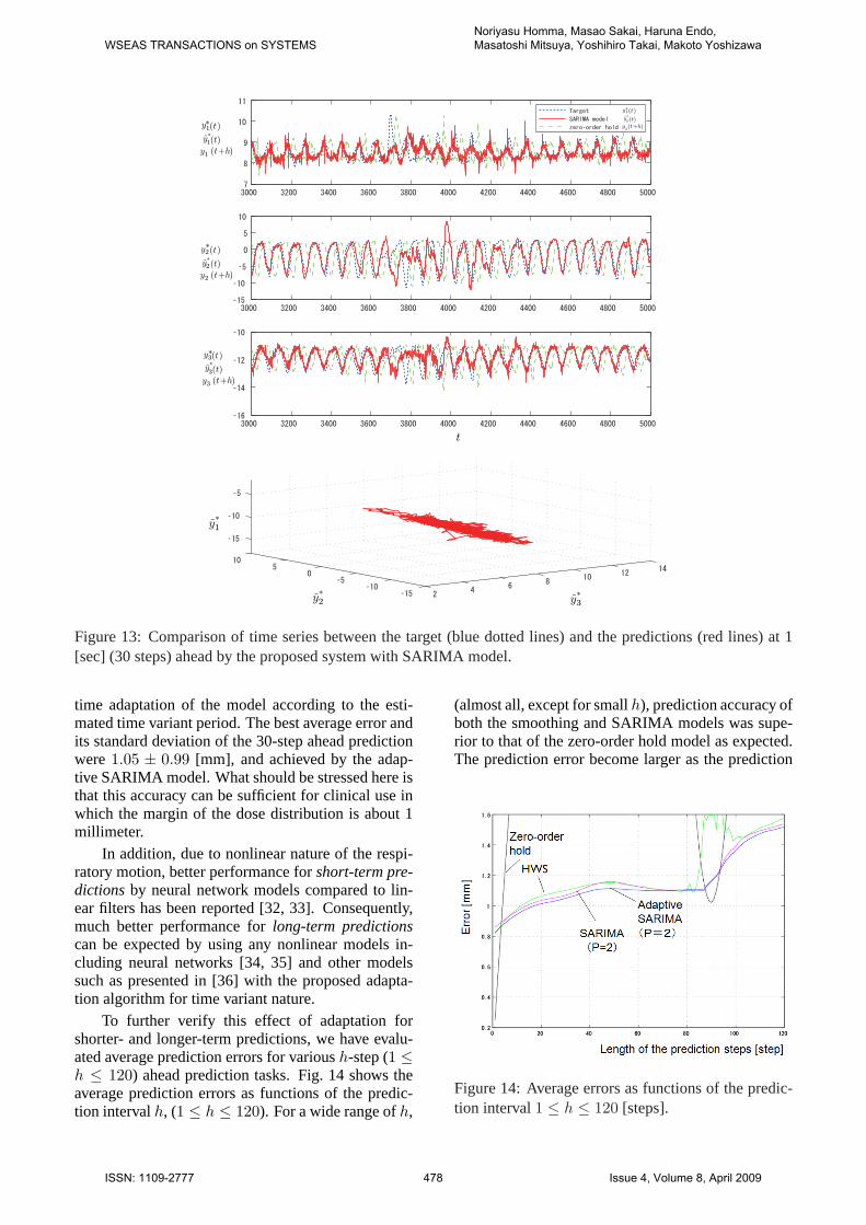
Figure 13:Comparison of time series between the target (blue dotted lines) and the predictions (red lines) at 1[sec] (30 steps) ahead by the proposed system with SARIMA model.

time adaptation of the model according to the esti-mated time variant period. The best average error andits standard deviation of the 30-step ahead predictionwere1.05 ± 0.99 [mm], and achieved by the adap-tive SARIMA model. What should be stressed here isthat this accuracy can be sufficient for clinical use inwhich the margin of the dose distribution is about 1millimeter.

In addition, due to nonlinear nature of the respi-ratory motion, better performance forshort-term pre-dictionsby neural network models compared to lin-ear filters has been reported [32, 33]. Consequently,much better performance forlong-term predictionscan be expected by using any nonlinear models in-cluding neural networks [34, 35] and other modelssuch as presented in [36] with the proposed adapta-tion algorithm for time variant nature.

To further verify this effect of adaptation forshorter- and longer-term predictions, we have evalu-ated average prediction errors for varioush-step (1≤h ≤ 120) ahead prediction tasks. Fig. 14 shows theaverage prediction errors as functions of the predic-tion intervalh, (1 ≤ h ≤ 120). For a wide range ofh,

(almost all, except for smallh), prediction accuracy ofboth the smoothing and SARIMA models was supe-rior to that of the zero-order hold model as expected.The prediction error become larger as the prediction

Figure 14:Average errors as functions of the predic-tion interval1 ≤ h ≤ 120 [steps].



intervals increase, but the best accuracy was againachieved by the adaptive SARIMA model. It can beconcluded that prediction accuracy within 1 [mm] bythe adaptive SARIMA model for shorter than 1 [sec]ahead prediction is a promising result for clinical use.

5 Conclusions

In this paper, we have developed time series predic-tion system for lung tumor motion tracking radiationtherapy. The precise prediction was achieved by theproposed technique based on the real-time adaptationto the time variant period involved in the cyclic dy-namics of respiration that may be a dominant sourceof the tumor motion. It is expected that such preciseprediction will reduce the adverse dosimetric effect ofthe tumor motion.

Simulation studies revealed the superior predic-tion performance of the proposed adaptation modelscompared to the conventional zero-order hold modeland that the prediction accuracy may be sufficientfor the clinical use. In addition to this, the fact thatthe performance of the proposed adaptive SARIMAmodel was further superior to that of the conven-tional SARIMA suggests the effectiveness of the pro-posed adaptation technique based on the predictionwith high accuracy.

Acknowledgements: This work was partially sup-ported by The Ministry of Education, Culture, Sports,Science and Technology under Grant-in-Aid for Sci-entific Research #19500413. Also, authors would liketo thank Dr. Shirato and his colleague at HokkaidoUniversity Hospital for sharing the clinical time se-ries data of human lung motion with us.

References:

[1] Wambersie A, Torsten Landberg, T, ICRU Re-port 62, Prescribing, Recording and ReportingPhoton Beam Therapy (Supplement to ICRUReport 50), ICRU News 1999.

[2] Onishi H, Araki T, Shirato H, et al., Stereo-tactic hypofractionated high-dose irradiation forstage I nonsmall cell lung carcinoma, Cancer,vol. 101, no. 7, pp. 1623-1631, 2004.

[3] G. A. Ezzellet al., “Guidance document on de-livery, treatment planning, and clinical imple-mentation of IMRT: Report of the IMRT sub-committee of AAPM radiation therapy commit-tee,” Medical Physics, vol. 30, pp. 2089-2115,2003.

[4] L. Xing, Q. Wu, Y. Yong, and A. L. Boyer, inPhysics of IMRT and Inverse Treatment Plan-ning in Intensity Modulated Radiation Therapy:A Clinical Perspective, edited by A. F. Mundtand J. C. Roeske, pp. 20-51, 2005.

[5] M. J. Murphy, “Tracking Moving Organs inReal Time,” Seminars in Radiation Oncology,vol. 14, no. 1, pp. 91-100, 2004.

[6] M. van Herk, “Errors and margins in radiationoncology,” Semin. Radiat. Oncol. vol. 14, pp.52-64, 2004.

[7] J. Hanleyet al., “Deep inspiration breath-holdtechnique for lung tumors: The potential valueof target immobilization and reduced lung den-sity in dose escalation,”Int. J. Radiat. Oncol.,Biol., Phys.vol. 45, pp. 603-611, 1999.

[8] H. D. Kuboet al., “Breathing-synchronized ra-diotherapy program at the University of Califor-nia Davis Cancer Center,”Med. Phys., vol. 27,pp. 346, 2000.

[9] S. S. Vedamet al., “Determining parameters forrespiration-gated radiotherapy,”Med. Phys., vol.28, pp. 2139-2146, 2001.

[10] X. A. Li, C. Stepaniak, and E. Gore, “Techni-cal and dosimetric aspects of respiratory gatingusing a pressure-sensor motion monitoring sys-tem,” Med. Phys., vol. 33, pp. 145-154, 2006.

[11] N. Wink et al., “Individualized gating windowsbased on fourdimensional CT information forrespiration gated radiotherapy,”Med. Phys., vol.34, pp. 2384, 2007.

[12] A. Schweikardet al., “Robotic motion compen-sation for respiratory movement during radio-surgery,”Comput. Aided Surg., vol. 5, pp. 263-277, 2000.

[13] P. J. Keallet al., “A four-dimensional controllerfor DMLC-based tumor tracking,”Int. J. Radiat.Oncol., Biol., Phys., vol. 60, pp. S338-S339,2004.

[14] C. Ozhasoglu, “Synchrony-Real-time respira-tory compensation system for the CyberKnife,”Med. Phys., vol. 33, pp. 2245-2246, 2006.

[15] P. J. Keallet al., “Motion adaptive x-ray therapy:A feasibility study,” Phys. Med. Biol., vol. 46,pp. 1-10, 2001.

[16] T. Neicuet al., “Synchronized moving apertureradiation therapy SMART: Average tumor tra-jectory for lung patients,”Phys. Med. Biol., vol.48, pp. 587-598, 2003.



[17] L. Papiez, “The leaf sweep algorithm for an im-mobile and moving target as an optimal controlproblem in radiotherapy delivery,”Math. Com-put. Modell., vol. 37, pp. 735-745, 2003.

[18] H. Shiratoet al., “Real-time tumor-tracking ra-diotherapy,” Lancet, vol. 353, pp. 1331-1332,1999.

[19] Y. Takai et al., “Development of a new linearaccelerator mounted with dual fluoroscopy us-ing amorphous silicon flat panel X-ray sensorsto detect a gold seed in a tumor at real treatmentposition,” Int. J. Radiat. Oncol. Biol. Phys., vol.51 (Supple.), pp. 381, 2001.

[20] R. I. Berbecoet al., “Integrated radiotherapyimaging system IRIS: Design considerations oftumour tracking with linac gantry-mounted di-agnostic x-ray systems with flat-panel detec-tors,” Phys. Med. Biol., vol. 49, pp. 243-255,2004.

[21] K. R. Britton et al., “Evaluation of inter-and in-trafraction organ motion during intensity mod-ulated radiation therapy (IMRT) for localizedprostate cancer measured by a newly developedon-board image-guided system,”Radiat. Med.,vol. 23, pp. 14-24, 2005.

[22] R. D. Wiersmaet al., “Combined kV and MVimaging for real-time tracking of implantedfiducial markers,”Med. Phys., vol. 35, pp. 1191-1198, 2008.

[23] H. D. Kubo and B. C. Hill, “Respiration gatedradiotherapy treatment: A technical study,”Phys. Med. Biol., vol. 41, pp. 83-91, 1996.

[24] C. Ozhasoglu and M. J. Murphy, “Issues in res-piratory motion compensation during external-beam radiotherapy,”Int. J. Radiat. Oncol., Biol.,Phys., vol. 52, pp. 1389-1399, 2002.

[25] L. Simon et al., “Lung volume assessment fora cross-comparison of two breathing-adaptedtechniques in radiotherapy,”Int. J. Radiat. On-col., Biol., Phys., vol. 63, pp. 602-609, 2005.

[26] P. R. Winters, “Forecasting Sales by Exponen-tially Weighted Moving Averages,”Manage-ment Science, vol. 6 pp. 324-342, 1960.

[27] G. E. P. Box, G. M. Jenkins,Time Series Anal-ysis, Forecasting and Control, Holden-Day, pp.1-553, 1970.

[28] Hokkaido University Hospital, Sapporo, Japan.http://www.huhp.hokudai.ac.jp/

[29] R. E. Kalman, “A New Approach to Linear Fil-tering and Prediction Problems,”T. ASME, J.Basic Engineering, Series D, vol. 83, pp. 35-45,1961.

[30] K. Akaike and G. Kitagawa,Practice in TimeSeries Analysis I, Asakura-Shoten, 2003 (inJapanese).

[31] Peter J. Brockwell and Richard A. Davis,In-troduction to Time Series and Forecasting,Springer Texts in Statistics, Springer, 1996.

[32] M. Isakssonet al., “On using an adaptive neu-ral network to predict lung tumor motion duringrespiration for radiotherapy applications,”Med.Phys., vol. 32, no. 12, pp. 3801-3809, 2005.

[33] M. J. Murphy and S. Dieterich, “Compara-tive performance of linear and nonlinear neuralnetworks to predict irregular breathing,”Phys.Med. Biol., vol. 51, pp. 5903-5914, 2006.

[34] Hazem M. El-Bakry and Nikos Mastorakis, “ANew Fast Forecasting Technique using HighSpeed Neural Networks,”WSEAS Trans. SignalProcessing, vol. 4, issue 10, pp. 573-595, 2008.

[35] Sanjay L. Badjate and Sanjay V. Dudul, “MultiStep Ahead Prediction of North and SouthHemisphere Sun Spots Chaotic Time Seriesusing Focused Time Lagged Recurrent Neu-ral Network Model,” WSEAS Trans. Informa-tion Science and Applications, vol. 6, issue 4,pp. 684-693, 2009.

[36] Miguel A. Garcia and Francisco Rodriguez,“An Iterative Algorithm for Automatic Fit-ting of Continuous Piecewise Linear Models,”WSEAS Trans. Signal Processing, vol. 4, issue8, pp. 474-483, 2008.



a new motion management method for lung tumor … · a new motion management method for lung tumor...

Documents