a new metric for quality of network community structure

A New Metric for Quality of Network Community Structure

Mingming ChenDepartment of Computer ScienceRensselaer Polytechnic Institute

110 8th StreetTroy, New York 12180Email: [email protected]

Tommy NguyenDepartment of Computer ScienceRensselaer Polytechnic Institute

110 8th StreetTroy, New York 12180

Email: [email protected]

Boleslaw K. SzymanskiDepartment of Computer ScienceRensselaer Polytechnic Institute

110 8th StreetTroy, New York 12180Email: [email protected]

ABSTRACT

Modularity is widely used to effectively measurethe strength of the community structure found bycommunity detection algorithms. However, modu-larity maximization suffers from two opposite yetcoexisting problems: in some cases, it tends to favorsmall communities over large ones while in others,large communities over small ones. The latter ten-dency is known in the literature as the resolutionlimit problem. To address them, we propose to mod-ify modularity by subtracting from it the fractionof edges connecting nodes of different communitiesand by including community density into modularity.We refer to the modified metric as Modularity Den-sity and we demonstrate that it indeed resolves bothproblems mentioned above. We describe the motiva-tion for introducing this metric by using intuitivelyclear and simple examples. We also prove that thisnew metric solves the resolution limit problem. Fi-nally, we discuss the results of applying this metric,modularity, and several other popular communityquality metrics to two real dynamic networks. Theresults imply that Modularity Density is consistentwith all the community quality measurements butnot modularity, which suggests that Modularity Den-sity is an improved measurement of the communityquality compared to modularity.

I INTRODUCTION

Communities are the basic structures in sociology ingeneral and in social networks in particular. Theyhave been intensively researched for more than a halfof the century [1]. Community in sociology usuallyrefers to a social unit whose members share commonvalues and the identity of the members as well astheir degree of cohesiveness depend on individuals’social and cognitive factors such as beliefs, prefer-ences, or needs. The ubiquity of the Internet andsocial media eliminated spatial limitations on com-munity geographical range, enabling on-line commu-nities to link people regardless of their physical loca-tion. The newly arising computational sociology re-

lies on computationally intensive methods to analyzeand model social phenomena [2], including communi-ties and their detection.

Analysis of social networks became one of the basictools of sociology [3] and has been used for linkingmicro and macro levels of sociological theory. Theclassical example of the approach is presented in [4]that elaborated the macro implications of one as-pect of small-scale interaction, the strength of dyadicties. Moreover, a lot of commercial applications, suchas digital marketing, behavioral targeting, and userpreference mining, rely heavily on community analy-sis. With the rapid growth of large-scale on-line socialnetworks, e.g., Facebook connected a billion users in2012, there is a high demand for efficient communitydetection algorithms that will be able to handle theirevolution growth. Communities in on-line social net-works are discovered by analyzing the observed andoften recorded on-line interactions between people.

In computational sociology, communities are definedas groups of nodes in a social network within whichconnections are denser than between them [5]. Thisdefinition has been found useful also in other typeof networks, and community detection became oneof the fundamental issues in network science. Com-munity detection has been shown to reveal latentyet meaningful structure not only for groups in on-line and contact-based social networks, but also ingroups of customers with similar interests in onlineretailer user networks, groups of scientists in inter-disciplinary collaboration networks, and in biologyin functional modules in protein-protein interactionnetworks etc. [6]. Since in most applications the realcommunities are not known (often due to the cost ofestablishing ground truth in large on-line social net-works), there is a need for developing reliable metricsto evaluate detected communities, so these metricscan be used to rank the quality of community struc-tures discovered by different community detection al-gorithms. Such metrics can also be used to developnovel community algorithms that iteratively attemptto improve the metrics by merging or splitting thegiven network community structure.

of 15c⃝ASE 2012

ASE Human Journal, vol. 2(4), 2013, pp. 226-240

In the last decade, the most popular community de-tection method, proposed by Newman [7], has beento maximize the quality metric known as modular-ity [5,8] over all the possible partitions of a network.This metric measures the difference (relative to thetotal number of edges) between the actual and ex-pected (in a randomized graph with the same numberof nodes and the same degree distribution) number ofedges within a given community. It is widely used tomeasure the strength of the community structures de-tected by the community detection algorithms. How-ever, modularity maximization has two opposite yetconcurrent problems. In some cases, it tends to splitlarge communities into smaller communities. In othercases, it tends to form large communities by mergingcommunities that are smaller than a certain thresholdwhich depends on the total number of edges in thenetwork and on the degree of inter-connectivity be-tween the communities. The latter problem is knownas the resolution limit problem [9].

To solve these two problems simultaneously, we pro-pose a new community quality metric, that we termedModularity Density, as an alternative to modularity.First, we show modularity decreased by Split Penalty,defined as the fraction of edges that connect nodes ofdifferent communities, solves the problem of favoringsmall communities. Next, we demonstrate that in-cluding community density into modularity addressesthe problem of favoring large communities. We referto the resulting metric as Modularity Density.

We formally prove that Modularity Density could re-solve the resolution limit problem. We also discussour experiments with this metric, modularity, andother popular community quality metrics, includingthe number of Intra-edges, Contraction, the num-ber of Inter-edges, Expansion, and Conductance [10],on two real dynamic networks. The results showthat Modularity Density is different from originalmodularity, but consistent with all those communityquality measurements, which implies that Modular-ity Density is effective in measuring the communityquality of networks.

The rest of the paper is organized as follows. First, inSection II we discuss some related works. Then, webriefly introduce modularity and illustrate our mo-tivation to propose the new metric with examples inSection III. Section IV presents the formal proofs andthe experiments that demonstrate Modularity Den-sity solves the two problems of modularity simulta-neously. Finally, we conclude and discuss the futurework in Section V.

II RELATED WORK

Community detection in complex networks has re-ceived a considerable amount of attention in the lastyears. Numerous techniques have been developed forboth efficient and effective community detection, in-cluding Modularity Optimization [7,8,11–15], CliquePercolation [16, 17], Local Expansion [18–20], FuzzyClustering [21, 22], Link Partitioning [23], and La-bel Propagation [24–26]. The above algorithms aredesigned to detect communities on static networks.However, networks, such as Internet and online socialnetworks, are usually dynamic, with changes arriv-ing as a stream. Thus, a large number of algorithmswere proposed to cope with community detection ondynamically evolving networks, such as LabelRankT[27] and Estrangement [28]. LabelRankT [27] detectscommunities in large-scale dynamic networks throughstabilized label propagation. Estrangement [28] de-tects temporal communities by maximizing modular-ity in a snapshot subject to a constraint on the es-trangement from the partition in the previous snap-shot.

In addition to the development of algorithms for com-munity detection, several metrics for evaluating thequality of community structure have been introduced.The most popular and widely used is modularity [5,8].It is defined as the difference (relative to the totalnumber of edges) between the actual and expected (ina randomized graph with the same number of nodesand the same degree sequence) number of edges insidea given community. Although initially defined for un-weighted and undirected networks, the definition ofmodularity has been subsequently extended to cap-ture community structure in weighted networks [29]and then in directed networks [30].

However, recently, Fortunato and Barthelemy [9]presented a resolution limit problem of modularity,essence of which is that optimizing modularity willnot find communities smaller than a threshold size,or weight [31]. This threshold depends on the to-tal number, or total weight, of edges in the net-work and on the degree of interconnectedness be-tween the communities. Moreover, Good et al. [32]shown that the range of modularity values computedover all possible partitions of a graph has a struc-ture in which the maximum modularity partition istypically concealed among an exponentially large (interms of the graph size) number of structurally dis-similar, high-modularity partitions. To address thisresolution limit problem, multi-resolution versions ofmodularity [33,34] were proposed to allow researchers

of 15c⃝ASE 2012

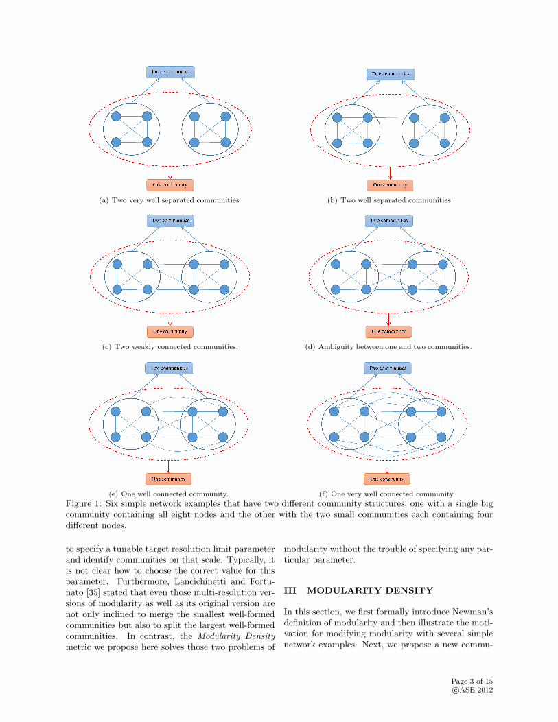
(a) Two very well separated communities. (b) Two well separated communities.

(c) Two weakly connected communities. (d) Ambiguity between one and two communities.

(e) One well connected community. (f) One very well connected community.

Figure 1: Six simple network examples that have two different community structures, one with a single bigcommunity containing all eight nodes and the other with the two small communities each containing fourdifferent nodes.

to specify a tunable target resolution limit parameterand identify communities on that scale. Typically, itis not clear how to choose the correct value for thisparameter. Furthermore, Lancichinetti and Fortu-nato [35] stated that even those multi-resolution ver-sions of modularity as well as its original version arenot only inclined to merge the smallest well-formedcommunities but also to split the largest well-formedcommunities. In contrast, the Modularity Densitymetric we propose here solves those two problems of

modularity without the trouble of specifying any par-ticular parameter.

III MODULARITY DENSITY

In this section, we first formally introduce Newman’sdefinition of modularity and then illustrate the moti-vation for modifying modularity with several simplenetwork examples. Next, we propose a new commu-

of 15c⃝ASE 2012

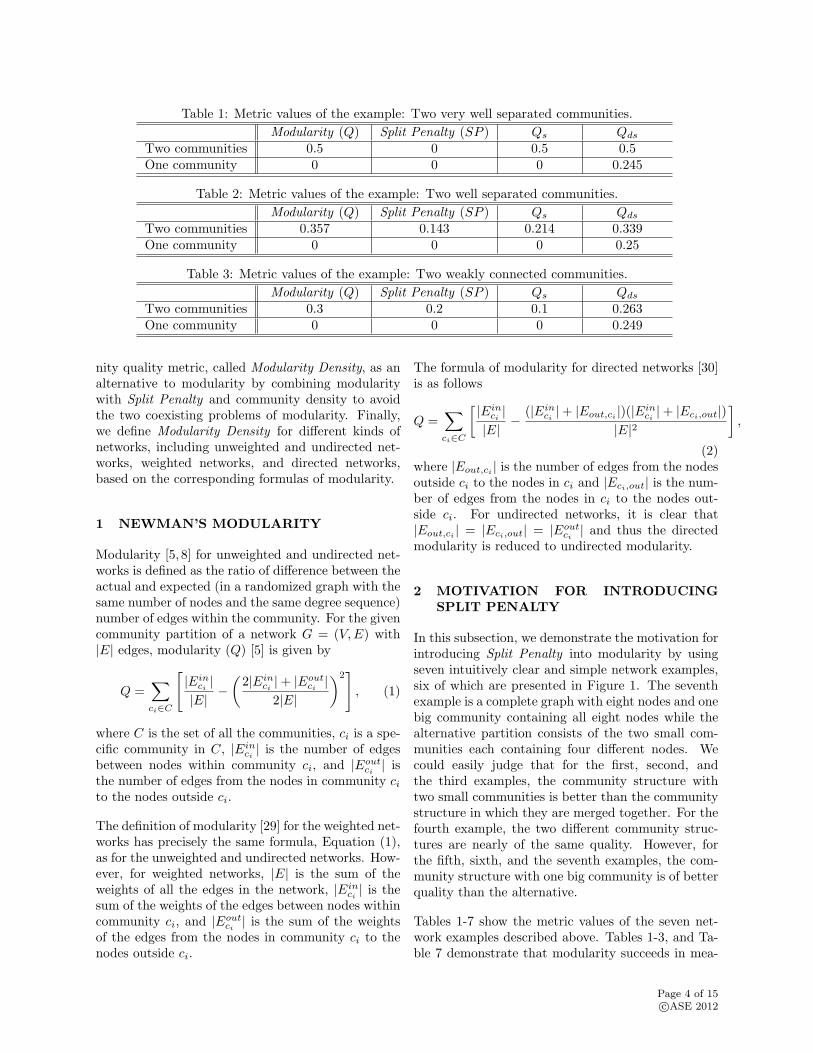
Table 1: Metric values of the example: Two very well separated communities.

Modularity (Q) Split Penalty (SP ) Qs Qds

Two communities 0.5 0 0.5 0.5One community 0 0 0 0.245

Table 2: Metric values of the example: Two well separated communities.


Two communities 0.357 0.143 0.214 0.339One community 0 0 0 0.25

Table 3: Metric values of the example: Two weakly connected communities.


Two communities 0.3 0.2 0.1 0.263One community 0 0 0 0.249

nity quality metric, called Modularity Density, as analternative to modularity by combining modularitywith Split Penalty and community density to avoidthe two coexisting problems of modularity. Finally,we define Modularity Density for different kinds ofnetworks, including unweighted and undirected net-works, weighted networks, and directed networks,based on the corresponding formulas of modularity.

1 NEWMAN’S MODULARITY

Modularity [5, 8] for unweighted and undirected net-works is defined as the ratio of difference between theactual and expected (in a randomized graph with thesame number of nodes and the same degree sequence)number of edges within the community. For the givencommunity partition of a network G = (V,E) with|E| edges, modularity (Q) [5] is given by

Q =∑ci∈C

[|Ein

ci ||E|

−(2|Ein

ci |+ |Eoutci |

2|E|

)2], (1)

where C is the set of all the communities, ci is a spe-cific community in C, |Ein

ci | is the number of edgesbetween nodes within community ci, and |Eout

ci | isthe number of edges from the nodes in community cito the nodes outside ci.

The definition of modularity [29] for the weighted net-works has precisely the same formula, Equation (1),as for the unweighted and undirected networks. How-ever, for weighted networks, |E| is the sum of theweights of all the edges in the network, |Ein

ci | is thesum of the weights of the edges between nodes withincommunity ci, and |Eout

ci | is the sum of the weightsof the edges from the nodes in community ci to thenodes outside ci.

The formula of modularity for directed networks [30]is as follows

Q =∑ci∈C

[ |Einci |

|E|−

(|Einci |+ |Eout,ci |)(|Ein

ci |+ |Eci,out|)|E|2

],

(2)where |Eout,ci | is the number of edges from the nodesoutside ci to the nodes in ci and |Eci,out| is the num-ber of edges from the nodes in ci to the nodes out-side ci. For undirected networks, it is clear that|Eout,ci | = |Eci,out| = |Eout

ci | and thus the directedmodularity is reduced to undirected modularity.

2 MOTIVATION FOR INTRODUCINGSPLIT PENALTY

In this subsection, we demonstrate the motivation forintroducing Split Penalty into modularity by usingseven intuitively clear and simple network examples,six of which are presented in Figure 1. The seventhexample is a complete graph with eight nodes and onebig community containing all eight nodes while thealternative partition consists of the two small com-munities each containing four different nodes. Wecould easily judge that for the first, second, andthe third examples, the community structure withtwo small communities is better than the communitystructure in which they are merged together. For thefourth example, the two different community struc-tures are nearly of the same quality. However, forthe fifth, sixth, and the seventh examples, the com-munity structure with one big community is of betterquality than the alternative.

Tables 1-7 show the metric values of the seven net-work examples described above. Tables 1-3, and Ta-ble 7 demonstrate that modularity succeeds in mea-

of 15c⃝ASE 2012

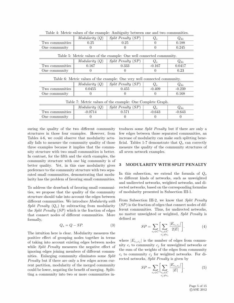
Table 4: Metric values of the example: Ambiguity between one and two communities.


Two communities 0.25 0.25 0 0.188One community 0 0 0 0.245

Table 5: Metric values of the example: One well connected community.


Two communities 0.167 0.333 -0.167 0.0417One community 0 0 0 0.23

Table 6: Metric values of the example: One very well connected community.


Two communities 0.0455 0.455 -0.409 -0.239One community 0 0 0 0.168

Table 7: Metric values of the example: One Complete Graph.


Two communities -0.0714 0.571 -0.643 -0.643One community 0 0 0 0

suring the quality of the two different communitystructures in those four examples. However, fromTables 4-6, we could observe that modularity actu-ally fails to measure the community quality of thosethree examples because it implies that the commu-nity structure with two small communities is better.In contrast, for the fifth and the sixth examples, thecommunity structure with one big community is ofbetter quality. Yet, in this case modularity givespreference to the community structure with two sepa-rated small communities, demonstrating that modu-larity has the problem of favoring small communities.

To address the drawback of favoring small communi-ties, we propose that the quality of the communitystructure should take into account the edges betweendifferent communities. We introduce Modularity withSplit Penalty (Qs) by subtracting from modularitythe Split Penalty (SP ) which is the fraction of edgesthat connect nodes of different communities. Moreformally,

Qs = Q− SP. (3)

The intuition here is clear. Modularity measures thepositive effect of grouping nodes together in termsof taking into account existing edges between nodeswhile Split Penalty measures the negative effect ofignoring edges joining members of different commu-nities. Enlarging community eliminates some SplitPenalty but if there are only a few edges across cur-rent partition, modularity of the merged communitycould be lower, negating the benefit of merging. Split-ting a community into two or more communities in-

troduces some Split Penalty but if there are only afew edges between those separated communities, anincrease of modularity can make such splitting bene-ficial. Tables 1-7 demonstrate that Qs can correctlymeasure the quality of the community structures ofall seven network examples.

3 MODULARITY WITH SPLIT PENALTY

In this subsection, we extend the formula of Qs

to different kinds of networks, such as unweightedand undirected networks, weighted networks, and di-rected networks, based on the corresponding formulasof modularity presented in Subsection III-1.

From Subsection III-2, we know that Split Penalty(SP ) is the fraction of edges that connect nodes of dif-ferent communities. Thus, for undirected networks,no matter unweighted or weighted, Split Penalty isdefined as

SP =∑ci∈C

[ ∑cj∈Ccj =ci

|Eci,cj |2|E|

]. (4)

where |Eci,cj | is the number of edges from commu-nity ci to community cj for unweighted networks orthe sum of the weights of the edges from communityci to community cj for weighted networks. For di-rected networks, Split Penalty is given by

SP =∑ci∈C

[ ∑cj∈Ccj =ci

|Eci,cj ||E|

]. (5)

of 15c⃝ASE 2012

(a) Two clique communities. (b) Two tree communities.

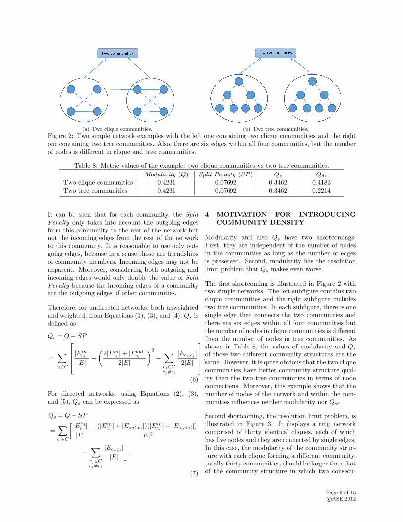
Figure 2: Two simple network examples with the left one containing two clique communities and the rightone containing two tree communities. Also, there are six edges within all four communities, but the numberof nodes is different in clique and tree communities.

Table 8: Metric values of the example: two clique communities vs two tree communities.


Two clique communities 0.4231 0.07692 0.3462 0.4183Two tree communities 0.4231 0.07692 0.3462 0.2214

It can be seen that for each community, the SplitPenalty only takes into account the outgoing edgesfrom this community to the rest of the network butnot the incoming edges from the rest of the networkto this community. It is reasonable to use only out-going edges, because in a sense those are friendshipsof community members. Incoming edges may not beapparent. Moreover, considering both outgoing andincoming edges would only double the value of SplitPenalty because the incoming edges of a communityare the outgoing edges of other communities.

Therefore, for undirected networks, both unweightedand weighted, from Equations (1), (3), and (4), Qs isdefined as

Qs = Q− SP

=∑ci∈C

|Einci |

|E|−

(2|Ein

ci |+ |Eoutci |

2|E|

)2

−∑cj∈Ccj =ci

|Eci,cj |2|E|

.

(6)

For directed networks, using Equations (2), (3),and (5), Qs can be expressed as

Qs = Q− SP

=∑ci∈C

[ |Einci |

|E|−

(|Einci |+ |Eout,ci |)(|Ein

ci |+ |Eci,out|)|E|2

−∑cj∈Ccj =ci

|Eci,cj ||E|

].

(7)

4 MOTIVATION FOR INTRODUCINGCOMMUNITY DENSITY

Modularity and also Qs have two shortcomings.First, they are independent of the number of nodesin the communities as long as the number of edgesis preserved. Second, modularity has the resolutionlimit problem that Qs makes even worse.

The first shortcoming is illustrated in Figure 2 withtwo simple networks. The left subfigure contains twoclique communities and the right subfigure includestwo tree communities. In each subfigure, there is onesingle edge that connects the two communities andthere are six edges within all four communities butthe number of nodes in clique communities is differentfrom the number of nodes in tree communities. Asshown in Table 8, the values of modularity and Qs

of those two different community structures are thesame. However, it is quite obvious that the two cliquecommunities have better community structure qual-ity than the two tree communities in terms of nodeconnections. Moreover, this example shows that thenumber of nodes of the network and within the com-munities influences neither modularity nor Qs.

Second shortcoming, the resolution limit problem, isillustrated in Figure 3. It displays a ring networkcomprised of thirty identical cliques, each of whichhas five nodes and they are connected by single edges.In this case, the modularity of the community struc-ture with each clique forming a different community,totally thirty communities, should be larger than thatof the community structure in which two consecu-

of 15c⃝ASE 2012

Figure 3: A ring network example made out of thirty identical cliques, each having five nodes and connectedby single edges.

Table 9: Metric values of the example: a ring of thirty cliques, each having five nodes and connected bysingle edges.


Thirty communities 0.8758 0.09091 0.7848 0.8721Fifteen communities 0.8879 0.04545 0.8424 0.4305

tive cliques form a different community, totally fifteencommunities. However, Table 9 shows that the rela-tion is reversed since the community structure withfifteen communities has larger modularity than thatof the community structure with thirty communities.Further, as pointed out in [9], when m(m−1)+2 < n,where n is the number of cliques and m is the numberof nodes in each clique, modularity is higher for thelarge community with two consecutive cliques insteadof the small community with a single clique. More-over, Table 9 demonstrates that the difference of Qs

for these two community structures is larger than thecorresponding difference of modularity. More specif-ically, ∆Qs = (0.8424 − 0.7848) = 0.0576 > ∆Q =(0.8879 − 0.8758) = 0.0121, which means that Qs

makes the resolution limit problem even worse.

To address the above two shortcomings, it is quiteintuitive to introduce community density into modu-larity, incorporating both the number of edges andthe number of nodes in the communities and alsoSplit Penalty. The corresponding new metric is calledModularity Density (Qds). Table 8 implies that theQds of the two tree communities is almost half ofthe Qds of the two clique communities. Moreover,Table 9 shows that the Qds of the community struc-ture in which two consecutive cliques form a differentcommunity is almost half of the Qds of the alterna-tive in which each clique forms a different commu-nity. Hence, in this case, Qds avoids the resolutionlimit problem. Furthermore, Tables 1-7 and Figure 1

demonstrate that Qds correctly measures the qualityof the community structures of all seven network ex-amples. Even for the network example of Figure 1(d)in which there is ambiguity which community struc-ture is of higher quality, the Qds of the one big com-munity is only slightly larger than the Qds of the twosmall communities as shown in Table 4.

5 MODULARITY DENSITY

In this subsection, we will give the formulas for Qds

for different kinds of networks, including unweightedand undirected networks, weighted networks, and di-rected networks, based on the corresponding formulasof Qs presented in Subsection III-3.

For undirected networks, regardless whether un-weighted or weighted, we define Qds using Equa-tion (6) as follows

Qds =∑ci∈C

[ |Einci |

|E|dci −

(2|Ein

ci |+ |Eoutci |

2|E|dci

)2

−∑cj∈Ccj =ci

|Eci,cj |2|E|

dci,cj

],

dci =2|Ein

ci ||ci|(|ci| − 1)

,

dci,cj =|Eci,cj ||ci||cj |

.

(8)

of 15c⃝ASE 2012

In the above, dci is the internal density of communityci, dci,cj is the pair-wise density between communityci and community cj . Note that |Ein

ci | in dci and|Eci,cj | in dci,cj are unweighted for both unweightedand weighted networks, so that those two communitydensities are always less than or equal to 1.0.

For directed networks, using Equation (7), Qds isgiven by

Qds =∑ci∈C

[ |Einci |

|E|dci

−(|Ein

ci |+ |Eout,ci |)(|Einci |+ |Eci,out|)

|E|2d2ci

−∑cj∈Ccj =ci

|Eci,cj ||E|

dci,cj

],

dci =|Ein

ci ||ci|(|ci| − 1)

,

dci,cj =|Eci,cj ||ci||cj |

.

(9)

IV EVALUATION AND ANALYSIS

In this section, we first prove that Modularity Den-sity (Qds) solves the resolution limit problem. Then,we introduce two real dynamic datasets and variousother popular community quality measurements. Fi-nally, we show the experimental results that validateQds ability to solve the two problems of modularity(Q) simultaneously.

1 PROOF OF SOLVING RESOLUTIONLIMIT PROBLEM

In this subsection, we test Modularity Density (Qds)on the examples from Fortunato and Barthelemy [9].First, we prove that Qds does not divide a clique intotwo or more parts. Then, we verify that Qds will notmerge two or more adjacent cliques connected with asingle edge. Finally, we prove that Qds can discovercommunities with different sizes.

Modularity Density (Qds) does not divide aclique into two or more parts. Given a cliquewith m (m ≥ 3) nodes, we prove that maximizingQds does not divide this clique into two parts. Con-sider an arbitrary partition P that divides the cliqueinto communities c1 and c2 with the number of nodesm1 and m2, respectively. Then, the number of edgesbetween c1 and c2 is m1m2. Let Qds(single) be the

Qds of the whole clique and Qds(pairs) be the Qds ofpartition P . By definitions,

Qds(single) = 0,

Qds(pairs) =(m1 −m2)

2 −m

m(m− 1)− m2

1 +m22

m2,

then,

Qds(pairs)−Qds(single) =−2m1m2 − 2m1m2m

m2(m− 1)< 0.

Hence, Qds will not divide a clique into two parts. Asimple generalization of this proof demonstrates thatQds will not divide a clique into three or more parts.

Modularity Density (Qds) does not merge twoor more consecutive cliques in the clique struc-ture ring network. Given a network, see Fig-ure 4(a), comprised of a ring of n (where n ≥ 2 is aneven integer) cliques connected through single edges.Each clique is a complete graph with m (m ≥ 3)nodes andm(m−1)/2 edges. Then, the cycle networkhas a total of nm nodes and nm(m− 1)/2+n edges.It is clear that the ring network has a well-formedcommunity structure where each community corre-sponds to a single clique. However, this communitystructure cannot be obtained by maximizing mod-ularity [9] since the community structure with n/2communities of two adjacent cliques each has highermodularity. We prove that maximizing Qds finds theright community structure. We letQds(single) be theQds of the community structure in which each cliqueis a different community, totally n communities, andQds(pairs) be the Qds of the community structurewith two consecutive cliques forming a different com-munity, totally n/2 communities. By definitions,

Qds(single) =m(m− 1)

m(m− 1) + 2− 1

n− 2

m3(m− 1) + 2m2,

Qds(pairs) =[m(m− 1) + 1]

2

[m(m− 1) + 2] [m(2m− 1)]

− 2 [m(m− 1) + 1]2

n [m(2m− 1)]2 − 1

4m3(m− 1) + 8m2.

We need to prove the inequality

Qds(pairs) < Qds(single). (10)

The first term of Qds(pairs) can be rewritten as

[m(m− 1) + 1]2

[m(m− 1) + 2][m(2m− 1)]=

m4 − 2m3 + 3m2 − 2m+ 1

m(m2 −m+ 2)(2m− 1).

Then, the first and third terms of Qds(single) withthe latter combined with the last term of Qds(pairs)yield

− m2 −m

m2 −m+ 2+

7

4m2(m2 −m+ 2)= − m4 −m3 − 1.75

m2(m2 −m+ 2).

of 15c⃝ASE 2012

Figure 4: Two clique structure network examples. (a) A clique structure ring network. There are totally n(where n is an even positive integer) cliques. Each clique contains m (m ≥ 3) nodes, and two consecutivecliques are connected by a single edge. (b) A network with two pairs of identical cliques. One pair of cliqueshave m (m ≥ 4) nodes, and the other pair of cliques have p (3 ≤ p < m) nodes.

Combining all these terms, we get

−m5 +m4 + 2m3 − 2m2 + 4.5m− 1.75

m2(m2 −m+ 2)(2m− 1).

We move the remaining two terms to the right handside of Inequality (10) that we are proving getting

1

n

−2m4 + 5m2 − 4m+ 2

m2(2m− 1)2.

Multiplying both sides by −m2(2m− 1) (and chang-ing direction of inequality) we get

m5 −m4 − 2m3 + 2m2 − 4.5m+ 1.75

m2 −m+ 2

>1

4n

m4 − 2.5m2 + 2m− 1

m− 0.5.

By doing divisions on both sides, we get

m3 − 4m− 2 +1.5m+ 5.75

m2 −m+ 2

>1

4n

[m3 + 0.5m2 − 2.25m+ 0.875− 9

16m− 8

].

Since 1.5m+5.75m2−m+2 ≥ 0, and 1

4n ≤ 18 for n ≥ 2 and also

916m−8 > 0, we just need to show that

m3 − 4m− 2 >m3 + 0.5m2 − 2.25m+ 0.875

8

which simplifies to

7m3 − 0.5m2 − 29.75m− 16.875 > 0 for m ≥ 3,

which is easy to prove either by induction, startingat m = 3, or by inspecting zeros of the derivative

21m2 −m− 29.75, which are all less than 2.0, show-ing that this polynomial is positive for m ≥ 3.

Since Inequality (10) holds, Qds will not merge twoconsecutive cliques in the ring network. A straight-forward extension of the proof shows that Qds willnot merge three or more consecutive cliques.

Modularity Density (Qds) could discover com-munities with different sizes. Consider a net-work, shown in Figure 4(b), with two pairs of identi-cal cliques. The left pair of cliques have m (m ≥ 4)nodes, and the right pair of cliques have p (3 ≤ p <m) nodes. This network has 2m + 2p nodes andm(m − 1) + p(p − 1) + 4 edges. It is obvious thateach of the four cliques should be a different commu-nity. However, the authors in [9] found that max-imizing modularity will merge the right two smallcliques. Here, we prove that maximizing Qds will notmerge them. We let Qds(single) denote the Qds ofthe community structure in which each clique corre-sponds to a single clique, and Qds(pairs) be the Qds

of the community structure with the right two smallcliques merged into one community. Clearly, the Qds

of the left two large cliques will stay the same in thosetwo different community structures so we denote it asQds(0). By definitions,

Qds(single) = Qds(0) +p(p− 1)

m(m− 1) + p(p− 1) + 4

− [p(p− 1) + 2]2

2 [m(m− 1) + p(p− 1) + 4]2

− 1

mp [m(m− 1) + p(p− 1) + 4]

− 1

p2 [m(m− 1) + p(p− 1) + 4],

of 15c⃝ASE 2012

Qds(pairs) = Qds(0)−1

mp [m(m− 1) + p(p− 1) + 4]

− [p(p− 1) + 1]2[p(p− 1) + 2]

2

p2(2p− 1)2 [m(m− 1) + p(p− 1) + 4]2

+[p(p− 1) + 1]

2

p(2p− 1) [m(m− 1) + p(p− 1) + 4].

The inequality that we need to prove is

Qds(single)−Qds(pairs) > 0. (11)

Since

Qds(single)−Qds(pairs)

=1

m(m− 1) + p(p− 1) + 4∗{p(p− 1)− 1

p2

− [p(p− 1) + 2]2

2[m(m− 1) + p(p− 1) + 4]− [p(p− 1) + 1]2

p(2p− 1)

+[p(p− 1) + 1]2[p(p− 1) + 2]2

p2(2p− 1)2[m(m− 1) + p(p− 1) + 4]

},

it is clear that the first factor is always positive so itcan be removed from consideration and the interiorof the second factor can be rewritten as

(p2 − p)+

2[p2 − p+ 1]2[p2 − p+ 2]2 − [p2 − p+ 2]2p2(2p− 1)2

2p2(2p− 1)2[m2 −m+ p2 − p+ 4]

>1

p2+

[p2 − p+ 1]2

p(2p− 1).

The second term simplifies to

− [p2 − p+ 2]2

2

2p4 − 5p2 + 4p− 2

p2(2p− 1)2[m2 −m+ p2 − p+ 4].

Since by induction for p ≥ 3 the polynomial 2p4 −5p2+4p−2 is positive, then this term is greater than

− (p2 − p+ 2)(2p4 − 5p2 + 4p− 2)

4p2(2p− 1)2

=1

4

[−0.5p2 + 0.375− 7.5p3 − 15.625p2 + 10p− 4

4p4 − 4p3 + p2

].

It is easy to show that the last fraction is less than0.391 by using induction or by finding zeros of thefraction derivative, which are all less than 2.5, so wejust need to prove that 0.875p2 − p− 0.004 is greaterthan the right hand side of Inequality (11).

The second term of the right hand side of Inequality(11) can be rewritten as

p4 − 2p3 + 3p2 − 2p+ 1

2(p2 − 0.5p)= 0.5p2 − 0.75p+ 1.125

− 0.875p− 1

2(p2 − 0.5p)< 0.5p2 − 0.75p+ 1.125,

because 0.875p > 1 and p2 > p for p ≥ 2.

Since 1p2 < 0.12, the inequality that we need to

prove reduces to 0.375p2 − 0.25p > 1.249, but forp ≥ 3, 0.375p2 − 0.25p ≥ 2.625, proving Inequality(11). Thus, we conclude that maximizing Qds willnot merge the right two small cliques, demonstratingthat Qds can discover communities of different size.

In summary, all the above proofs show that Modu-larity Density solves the resolution limit problem ofmodularity.

2 REAL DYNAMIC DATASETS

In this subsection, we introduce two real dynamicdatasets on which we conduct experiments in order tovalidate Qds avoids the two problems of modularity.

Senate Dataset [28, 36]. The Senate dataset is atime-evolving weighted network comprised of UnitedStates senators where the weight of an edge repre-sents the similarity of their roll call voting behavior.This dataset was obtained from website voteview.comand the similarities between a pair of senators werecalculated following Waugh et al. [36] as the num-ber of bills for which the senators of the pair votedthe same way, normalized by the number of bills forwhich they both voted. The dataset totally consistsof 111 snapshots corresponding to Senate’s activitiesover 220 years and includes 1916 unique senators.

Reality Mining Bluetooth Scan Data [37]. Thisdataset was created from the records of BluetoothScans generated among the 94 subjects in RealityMining study conducted from 2004-2005 at the MITMedia Laboratory. In the network, nodes representthe subjects and the directed edges correspond to theBluetooth Scan records while the weight of each edgerepresents the number of direct Bluetooth scans be-tween the two subjects. In the experiments, we onlyused the records from August 02, 2004 (Monday) toMay 29, 2005 (Sunday) and we divided them intoweekly snapshots, so each snapshot represents scanscollected during the corresponding week. There aretotal of 43 snapshots.

3 COMMUNITY QUALITY MEASURE-MENTS

In the discussion of the experimental results we usevarious community quality metrics, including the

of 15c⃝ASE 2012

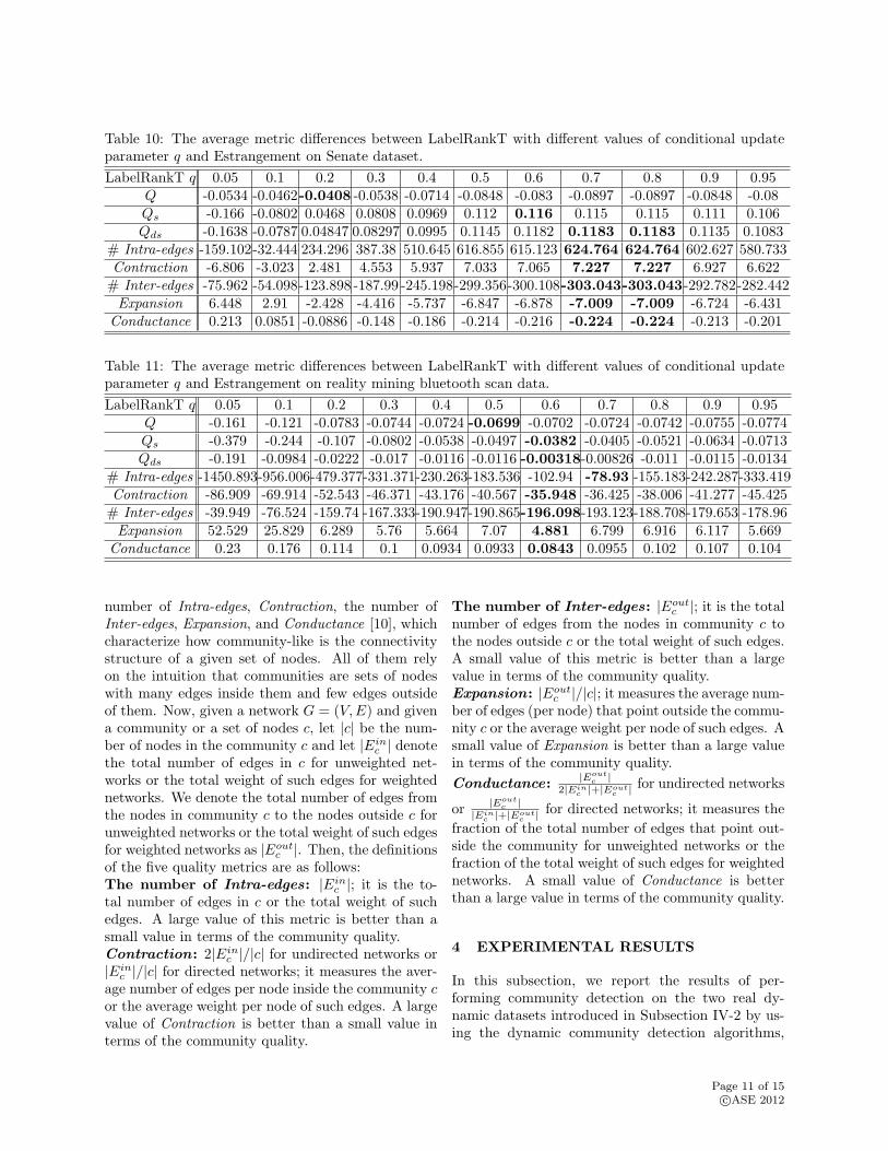
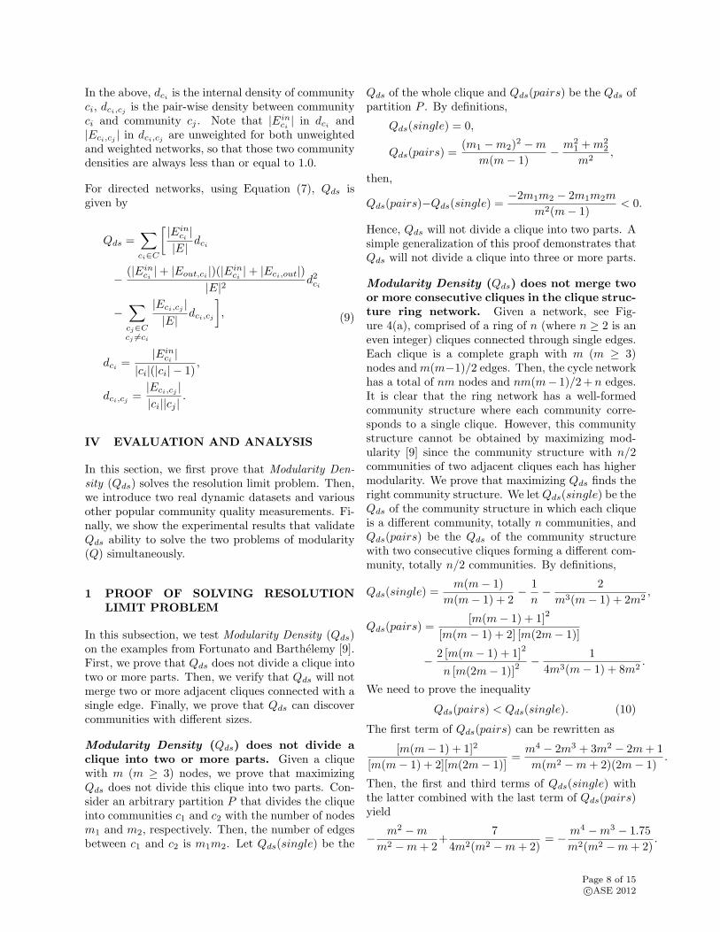
Table 10: The average metric differences between LabelRankT with different values of conditional updateparameter q and Estrangement on Senate dataset.

LabelRankT q 0.05 0.1 0.2 0.3 0.4 0.5 0.6 0.7 0.8 0.9 0.95Q -0.0534 -0.0462-0.0408 -0.0538 -0.0714 -0.0848 -0.083 -0.0897 -0.0897 -0.0848 -0.08Qs -0.166 -0.0802 0.0468 0.0808 0.0969 0.112 0.116 0.115 0.115 0.111 0.106Qds -0.1638 -0.0787 0.04847 0.08297 0.0995 0.1145 0.1182 0.1183 0.1183 0.1135 0.1083

# Intra-edges -159.102-32.444 234.296 387.38 510.645 616.855 615.123 624.764 624.764 602.627 580.733Contraction -6.806 -3.023 2.481 4.553 5.937 7.033 7.065 7.227 7.227 6.927 6.622# Inter-edges -75.962 -54.098-123.898 -187.99 -245.198-299.356-300.108-303.043-303.043-292.782-282.442Expansion 6.448 2.91 -2.428 -4.416 -5.737 -6.847 -6.878 -7.009 -7.009 -6.724 -6.431

Conductance 0.213 0.0851 -0.0886 -0.148 -0.186 -0.214 -0.216 -0.224 -0.224 -0.213 -0.201

Table 11: The average metric differences between LabelRankT with different values of conditional updateparameter q and Estrangement on reality mining bluetooth scan data.

LabelRankT q 0.05 0.1 0.2 0.3 0.4 0.5 0.6 0.7 0.8 0.9 0.95Q -0.161 -0.121 -0.0783 -0.0744 -0.0724 -0.0699 -0.0702 -0.0724 -0.0742 -0.0755 -0.0774Qs -0.379 -0.244 -0.107 -0.0802 -0.0538 -0.0497 -0.0382 -0.0405 -0.0521 -0.0634 -0.0713Qds -0.191 -0.0984 -0.0222 -0.017 -0.0116 -0.0116 -0.00318-0.00826 -0.011 -0.0115 -0.0134

# Intra-edges -1450.893-956.006-479.377-331.371-230.263-183.536 -102.94 -78.93 -155.183-242.287-333.419Contraction -86.909 -69.914 -52.543 -46.371 -43.176 -40.567 -35.948 -36.425 -38.006 -41.277 -45.425# Inter-edges -39.949 -76.524 -159.74 -167.333-190.947-190.865-196.098-193.123-188.708-179.653 -178.96Expansion 52.529 25.829 6.289 5.76 5.664 7.07 4.881 6.799 6.916 6.117 5.669

Conductance 0.23 0.176 0.114 0.1 0.0934 0.0933 0.0843 0.0955 0.102 0.107 0.104

number of Intra-edges, Contraction, the number ofInter-edges, Expansion, and Conductance [10], whichcharacterize how community-like is the connectivitystructure of a given set of nodes. All of them relyon the intuition that communities are sets of nodeswith many edges inside them and few edges outsideof them. Now, given a network G = (V,E) and givena community or a set of nodes c, let |c| be the num-ber of nodes in the community c and let |Ein

c | denotethe total number of edges in c for unweighted net-works or the total weight of such edges for weightednetworks. We denote the total number of edges fromthe nodes in community c to the nodes outside c forunweighted networks or the total weight of such edgesfor weighted networks as |Eout

c |. Then, the definitionsof the five quality metrics are as follows:The number of Intra-edges: |Ein

c |; it is the to-tal number of edges in c or the total weight of suchedges. A large value of this metric is better than asmall value in terms of the community quality.Contraction: 2|Ein

c |/|c| for undirected networks or|Ein

c |/|c| for directed networks; it measures the aver-age number of edges per node inside the community cor the average weight per node of such edges. A largevalue of Contraction is better than a small value interms of the community quality.

The number of Inter-edges: |Eoutc |; it is the total

number of edges from the nodes in community c tothe nodes outside c or the total weight of such edges.A small value of this metric is better than a largevalue in terms of the community quality.Expansion: |Eout

c |/|c|; it measures the average num-ber of edges (per node) that point outside the commu-nity c or the average weight per node of such edges. Asmall value of Expansion is better than a large valuein terms of the community quality.

Conductance:|Eout

c |2|Ein

c |+|Eoutc | for undirected networks

or|Eout

c ||Ein

c |+|Eoutc | for directed networks; it measures the

fraction of the total number of edges that point out-side the community for unweighted networks or thefraction of the total weight of such edges for weightednetworks. A small value of Conductance is betterthan a large value in terms of the community quality.

4 EXPERIMENTAL RESULTS

In this subsection, we report the results of per-forming community detection on the two real dy-namic datasets introduced in Subsection IV-2 by us-ing the dynamic community detection algorithms,

of 15c⃝ASE 2012

10 20 30 40 50 60 70 80 90 100 110−0.3

−0.2

−0.1

0

0.1

0.2

0.3

0.4

Snapshot

Mo

du

lari

ty

LabelRankTEstrangementDifference

(a) Senate dataset (q = 0.7).

5 10 15 20 25 30 35 40−0.8

−0.6

−0.4

−0.2

0

0.2

0.4

0.6

0.8

1

Snapshot

Mo

du

lari

ty


(b) Reality Mining Bluetooth Scan data (q = 0.6).

Figure 5: The modularity (Q) of the community detection results of LabelRankT and Estrangement (also,the difference between LabelRankT and Estrangement) on (a) each snapshot of Senate dataset at q = 0.7and on (b) each snapshot of Reality Mining Bluetooth Scan data with q = 0.6.

LabelRankT [27] and Estrangement [28]. We chosethese two algorithms because the second algorithmrelies on the modularity optimization while the firstone does not. In the experiments, we adopted thebest parameter of Estrangement but varying the con-ditional update parameter q ∈ [0, 1] of LabelRankTfrom 0.05 to 0.95. As seen in the results, in mostcases, the best q is around 0.7 in agreement withthe best value reported in [27]. For the communitystructures found by the two algorithms, we calculatedthe values of modularity (Q), Qs, Modularity Den-sity (Qds), and the five community quality metricsdescribed in Subsection IV-3.

Table 10 and Table 11 present the average metric dif-ferences between LabelRankT with different values ofconditional update parameter q and Estrangement onSenate dataset and Reality Mining Bluetooth Scandata, respectively. That is, we first computed thevalues of the eight metrics above for the communitydetection results, detected by Estrangement, of eachsnapshot. Then, we calculated the eight metrics val-ues for the community detection results, discoveredby LabelRankT for all q, of each snapshot. Next,we got the metric differences of all eight metrics bysubtracting the metric values of Estrangement fromthose of LabelRankT for all q’s over each snapshot.Then, averaging those differences of each metric overall the snapshots, we obtained the corresponding av-erage metric differences.

Table 10 demonstrates that Q gets its largest valuewhen q = 0.2; Qs reaches the largest value whenq = 0.6; Qds, Intra-edges, and Contraction get theirlargest values at q = 0.7 and q = 0.8; also, Inter-edges, Expansion, and Conductance reach their small-

est values at q = 0.7 and q = 0.8. Thus, Qds isconsistent with the five metrics introduced in Subsec-tion IV-3 on determining the best q for LabelRankTon Senate dataset while Q and Qs are not consis-tent with them. Further, we could observe that Qis always negative which indicates that LabelRankTperforms below Estrangement over all q’s becausethe goal of Estrangement is to maximize modularity(Q). However, the other seven metrics imply that La-belRankT performs better than Estrangement whenq > 0.1. Therefore, we could explicitly observe thatmaximizing Q to detect communities has problems inmeasuring the community detection quality correctlyon Senate dataset.

Table 11 shows that six metrics get their best (largestor smallest) values at q = 0.6 while the two excep-tions, Q and the number of Intra-edges, reach theirlargest values when q = 0.5 and q = 0.7, respec-tively. Thus, the six metrics, except Q and the num-ber of Intra-edges, are consistent on determining thebest value of q for LabelRankT on Reality MiningBluetooth Scan data. This indicates that on RealityMining Bluetooth Scan data, maximizing Q to detectcommunities has problems.

It is also interesting to observe that for q = 0.05and q = 0.1 in Table 10, Inter-edges metric impliesthat LabelRankT performs better than Estrangementon Senate dataset, which is not consistent with Qs,Qds, Intra-edges, Contraction, Expansion, and Con-ductance metrics. Moreover, we could learn from Ta-ble 11 that all the metrics, except Inter-edges met-ric, imply that LabelRankT performs slightly belowthe performance of Estrangement over all q’s. Thus,Inter-edges metric has some problems. Also, as men-

of 15c⃝ASE 2012

10 20 30 40 50 60 70 80 90 100 110−0.5

−0.4

−0.3

−0.2

−0.1

0

0.1

0.2

0.3

0.4

0.5

Snapshot

Qs



5 10 15 20 25 30 35 40−0.8

−0.6

−0.4

−0.2

0

0.2

0.4

0.6

0.8

Snapshot

Qs



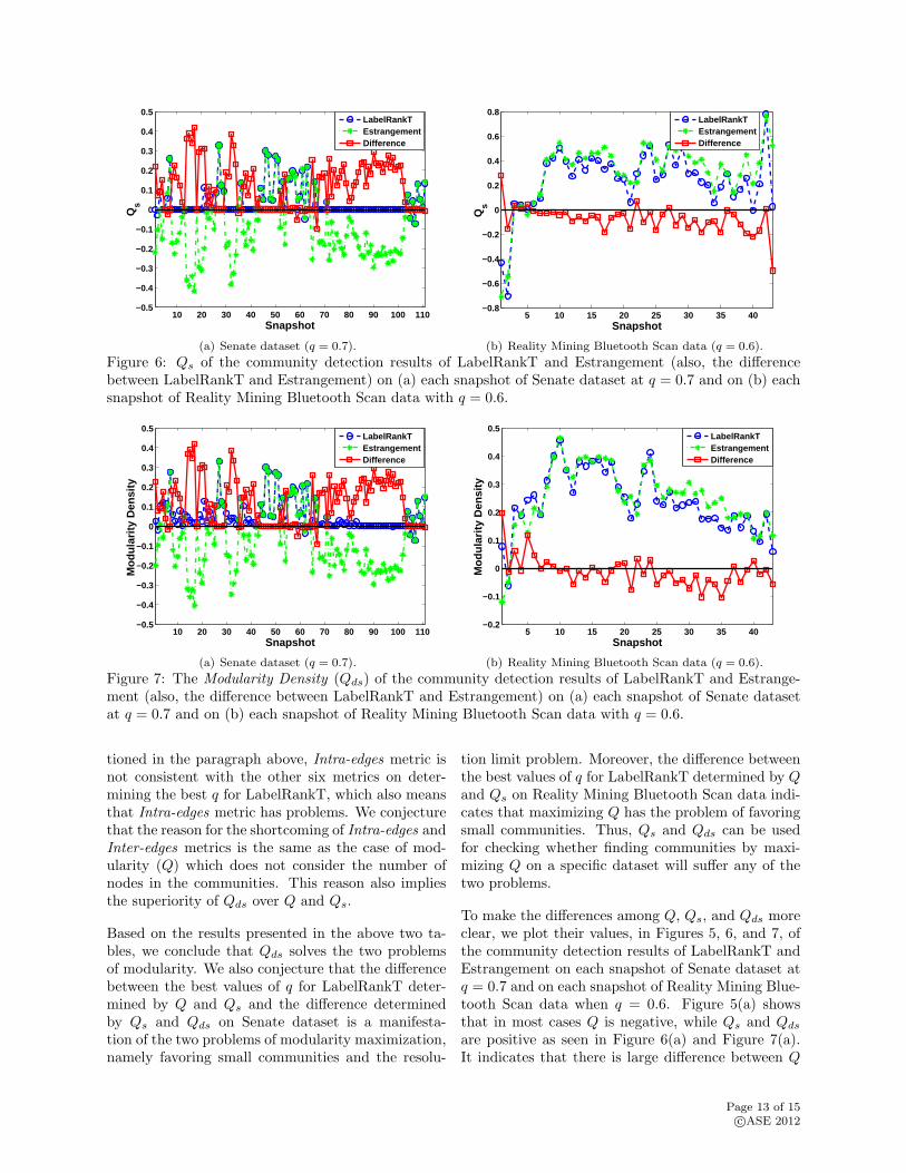
Figure 6: Qs of the community detection results of LabelRankT and Estrangement (also, the differencebetween LabelRankT and Estrangement) on (a) each snapshot of Senate dataset at q = 0.7 and on (b) eachsnapshot of Reality Mining Bluetooth Scan data with q = 0.6.

10 20 30 40 50 60 70 80 90 100 110−0.5

−0.4

−0.3

−0.2

−0.1

0

0.1

0.2

0.3

0.4

0.5

Snapshot

Mo

du

lari

ty D

ensi

ty



5 10 15 20 25 30 35 40−0.2

−0.1

0

0.1

0.2

0.3

0.4

0.5

Snapshot

Mo

du

lari

ty D

ensi

ty



Figure 7: The Modularity Density (Qds) of the community detection results of LabelRankT and Estrange-ment (also, the difference between LabelRankT and Estrangement) on (a) each snapshot of Senate datasetat q = 0.7 and on (b) each snapshot of Reality Mining Bluetooth Scan data with q = 0.6.

tioned in the paragraph above, Intra-edges metric isnot consistent with the other six metrics on deter-mining the best q for LabelRankT, which also meansthat Intra-edges metric has problems. We conjecturethat the reason for the shortcoming of Intra-edges andInter-edges metrics is the same as the case of mod-ularity (Q) which does not consider the number ofnodes in the communities. This reason also impliesthe superiority of Qds over Q and Qs.

Based on the results presented in the above two ta-bles, we conclude that Qds solves the two problemsof modularity. We also conjecture that the differencebetween the best values of q for LabelRankT deter-mined by Q and Qs and the difference determinedby Qs and Qds on Senate dataset is a manifesta-tion of the two problems of modularity maximization,namely favoring small communities and the resolu-

tion limit problem. Moreover, the difference betweenthe best values of q for LabelRankT determined by Qand Qs on Reality Mining Bluetooth Scan data indi-cates that maximizing Q has the problem of favoringsmall communities. Thus, Qs and Qds can be usedfor checking whether finding communities by maxi-mizing Q on a specific dataset will suffer any of thetwo problems.

To make the differences among Q, Qs, and Qds moreclear, we plot their values, in Figures 5, 6, and 7, ofthe community detection results of LabelRankT andEstrangement on each snapshot of Senate dataset atq = 0.7 and on each snapshot of Reality Mining Blue-tooth Scan data when q = 0.6. Figure 5(a) showsthat in most cases Q is negative, while Qs and Qds

are positive as seen in Figure 6(a) and Figure 7(a).It indicates that there is large difference between Q

of 15c⃝ASE 2012

and Qs or between Q and Qds. This is consistentwith Table 10. Further, it can be observed from Fig-ure 6(a) and Figure 7(a) that Qs and Qds are almostthe same on each snapshot, which is also consistentwith Table 10. Figure 5(b), Figure 6(b), and Fig-ure 7(b) demonstrate that Q, Qs, and Qds are neg-ative in most of the cases, although their values aredifferent in each snapshot. These observations areconsistent with the results shown in Table 11.

V CONCLUSION AND FUTURE WORK

In this paper, we propose a new community qualitymetric, called Modularity Density, which solves theproblems of modularity of favoring small communi-ties in some circumstances and large communities inothers. We demonstrate with proofs and experimentson real dynamic datasets that Modularity Density isan effective alternative to modularity.

In the future, we plan to extend Modularity Den-sity to enable evaluation of the quality of overlap-ping community structures. We will also propose acommunity detection algorithm based on ModularityDensity maximization and then compare its commu-nity detection results with those of modularity max-imization algorithms on some typical real networks.

ACKNOWLEDGMENT

This work was supported in part by the ArmyResearch Laboratory under Cooperative AgreementNumber W911NF-09-2-0053 and by the the Office ofNaval Research Grant No. N00014-09-1-0607. Theviews and conclusions contained in this document arethose of the authors and should not be interpreted asrepresenting the official policies either expressed orimplied of the Army Research Laboratory or the U.S.Government.

References

[1] R. E. Park, Human communities: The city andhuman ecology, Free Press, New York, NY, 1952.

[2] W. S. Bainbridge, “Computational sociology”,in Blackwell Encyclopedia of Sociology, 2007.

[3] Stanley Wasserman and Katherine Faust, So-cial network analysis: Methods and applications,vol. 8, Cambridge University Press, Cambridge,U.K., 1994.

[4] M.S. Granovetter, “The Strength of Weak Ties”,The American Journal of Sociology, vol. 78, no.6, pp. 1360–1380, 1973.

[5] M. E. J. Newman and M. Girvan, “Finding andevaluating community structure in networks”,Phys. Rev. E, vol. 69, pp. 026113, Feb 2004.

[6] Santo Fortunato, “Community detection ingraphs”, Physics Reports, vol. 486, pp. 75–174,2010.

[7] M. E. J. Newman, “Fast algorithm for detectingcommunity structure in networks”, Phys. Rev.E, vol. 69, pp. 066133, Jun 2004.

[8] M. E. J. Newman, “Modularity and communitystructure in networks”, Proceedings of the Na-tional Academy of Sciences, vol. 103, no. 23, pp.8577–8582, 2006.

[9] Santo Fortunato and Marc Barthelemy, “Resolu-tion limit in community detection”, Proceedingsof the National Academy of Sciences, vol. 104,no. 1, pp. 36–41, 2007.

[10] Jaewon Yang and Jure Leskovec, “Defningand evaluating network communities based onground-truth”, IEEE International ConferenceOn Data Mining (ICDM), 2012.

[11] Aaron Clauset, M. E. J. Newman, and Cristo-pher Moore, “Finding community structure invery large networks”, Phys. Rev. E, vol. 70, pp.066111, Dec 2004.

[12] Vincent D Blondel, Jean-Loup Guillaume, Re-naud Lambiotte, and Etienne Lefebvre, “Fastunfolding of communities in large networks”,Journal of Statistical Mechanics: Theory andExperiment, vol. 2008, no. 10, pp. P10008, 2008.

[13] Thomas Richardson, Peter J. Mucha, and Ma-son A. Porter, “Spectral tripartitioning of net-works”, Phys. Rev. E, vol. 80, pp. 036111, Sep2009.

[14] Jordi Duch and Alex Arenas, “Community de-tection in complex networks using extremal op-timization”, Phys. Rev. E, vol. 72, pp. 027104,Aug 2005.

[15] Guimera R and Nunes Amaral LA, “Functionalcartography of complex metabolic networks”,Nature, vol. 433, pp. 895–900, FEB 2005.

[16] Gergely Palla, Imre Derenyi, Illes Farkas, andTamas Vicsek, “Uncovering the overlappingcommunity structure of complex networks in na-ture and society”, 2005.

of 15c⃝ASE 2012

[17] Illes Farkas, Daniel Abel, Gergely Palla, andTamas Vicsek, “Weighted network modules”,New Journal of Physics, vol. 9, no. 6, pp. 180,2007.

[18] Jeffrey Baumes, Mark Goldberg, and MalikMagdon-ismail, “Efficient identification of over-lapping communities”, in In IEEE InternationalConference on Intelligence and Security Infor-matics (ISI, 2005, pp. 27–36.

[19] Andrea Lancichinetti, Santo Fortunato, andJanos Kertesz, “Detecting the overlapping andhierarchical community structure in complexnetworks”, New Journal of Physics, vol. 11, no.3, pp. 033015, 2009.

[20] Huawei Shen, Xueqi Cheng, Kai Cai, and Mao-Bin Hu, “Detect overlapping and hierarchicalcommunity structure in networks”, Physica A:Statistical Mechanics and its Applications, vol.388, no. 8, pp. 1706–1712, 2009.

[21] Shihua Zhang, Rui-Sheng Wang, and Xiang-SunZhang, “Identification of overlapping commu-nity structure in complex networks using fuzzy-means clustering”, Physica A: Statistical Me-chanics and its Applications, vol. 374, no. 1, pp.483–490, 2007.

[22] Ioannis Psorakis, Stephen Roberts, Mark Ebden,and Ben Sheldon, “Overlapping community de-tection using bayesian non-negative matrix fac-torization”, Phys. Rev. E, vol. 83, pp. 066114,Jun 2011.

[23] Yong-Yeol Ahn, James P Bagrow, and SuneLehmann, “Link communities reveal multiscalecomplexity in networks”, Nature, vol. 466, no.7307, pp. 761–764, 2010.

[24] Usha Nandini Raghavan, Reka Albert, andSoundar Kumara, “Near linear time algorithmto detect community structures in large-scalenetworks”, Phys. Rev. E, vol. 76, pp. 036106,Sep 2007.

[25] Jierui Xie and Boleslaw K. Szymansk, “Com-munity detection using a neighborhood strengthdriven label propagation algorithm”, in IEEENSW 2011, 2011, pp. 188–195.

[26] Jierui Xie and Boleslaw K. Szymanski, “Towardslinear time overlapping community detection insocial networks”, in The 16th Pacific-Asia Con-ference on Knowledge Discovery and Data Min-ing (PAKDD), 2012, pp. 25–36.

[27] Jierui Xie, Mingming Chen, and Boleslaw K.Szymanski, “LabelrankT: Incremental commu-nity detection in dynamic networks via labelpropagation”, in ACM SIGMOD Workshopon Dynamic Networks Management and Mining(DyNetMM), New York, USA, 2013.

[28] Vikas Kawadia and Sameet Sreenivasan, “Se-quential detection of temporal communities byestrangement confinement”, Scientific Reports,vol. 2, November 2012.

[29] M. E. J. Newman, “Analysis of weighted net-works”, Phys. Rev. E, vol. 70, pp. 056131, Nov2004.

[30] E. A. Leicht and M. E. J. Newman, “Commu-nity structure in directed networks”, Phys. Rev.Lett., vol. 100, pp. 118703, Mar 2008.

[31] Jonathan W. Berry, Bruce Hendrickson, Ran-dall A. LaViolette, and Cynthia A. Phillips,“Tolerating the community detection resolutionlimit with edge weighting”, Phys. Rev. E, vol.83, pp. 056119, May 2011.

[32] Benjamin H. Good, Yves-Alexandre de Mon-tjoye, and Aaron Clauset, “Performance ofmodularity maximization in practical contexts”,Phys. Rev. E, vol. 81, pp. 046106, Apr 2010.

[33] Jorg Reichardt and Stefan Bornholdt, “Statis-tical mechanics of community detection”, Phys.Rev. E, vol. 74, pp. 016110, Jul 2006.

[34] A Arenas, A Fernandez, and S Gomez, “Analysisof the structure of complex networks at differentresolution levels”, New Journal of Physics, vol.10, no. 5, pp. 053039, 2008.

[35] Andrea Lancichinetti and Santo Fortunato,“Limits of modularity maximization in commu-nity detection”, Phys. Rev. E, vol. 84, pp.066122, Dec 2011.

[36] Andrew Scott Waugh, Liuyi Pei, James H.Fowler, Peter J. Mucha, and Mason A. Porter,“Party polarization in congress: A network sci-ence approach”, arXiv:0907.3509, 2010.

[37] Nathan Eagle, Alex Pentland, and David Lazer,“Inferring social network structure using mo-bile phone data”, Proceedings of the NationalAcademy of Sciences (PNAS), vol. 106, no. 36,pp. 15274–15278, 2009.

of 15c⃝ASE 2012

a new metric for quality of network community structure

Documents