A New Keynesian Framework with Unemployment and

Credible Bargaining: Positive and Normative Implications

Pierrick Clerc ∗

Paris School of Economics

Abstract

Sveen and Weinke (2008) argue that the capacity of real wage rigidities to mag-

nify unemployment fluctuations critically depends on the way hours per worker are

determined. Those rigidities would raise labor market volatility under the strong as-

sumption that hours are determined jointly by the employer and the worker, but would

loose this ability when hours are firms’s choices. This result challenges the role of real

wage stickiness in solving the unemployment volatility puzzle and providing a signif-

icant stabilization trade-off between inflation and unemployment. Here, I argue that

what is critical is instead the way real wage rigidities are introduced. I replace the

ad-hoc wage norm, usually retained to gererate that rigidities, by the micro-founded

credible bargaining into a New Keynesian model with search frictions. I find that this

framework sharply amplifies the unemployment dynamics and replicates a great part of

labor market standard deviations. Further, the zero inflation policy implies large and

inefficient unemployment fluctuations. Those results hold whatever the way of deter-

mining hours per worker. Real wage rigidities are therefore the required ingredient to

enhance labor market volatility and deliver a meaningful policy trade-off.

JEL Codes : E32, E50.

Keywords: New-Keynesian model, labor market frictions, unemployment, real wage rigidi-

ties.

∗Centre d’Economie de la Sorbonne, Paris School of Economics. Email : Pierrick.Clerc@malix.univ-

paris1.fr

1

1 Introduction

Real wage rigidities were advocated to provide a solution to both positive and normative

issues. On the positive side, Shimer (2005) and Hall (2005) argue that those rigidities

are the required feature to solve the unemployment volatility puzzle, i.e. the weak labor

market volatility produced by the canonical search and matching model1. On the normative

side, Blanchard and Galı (2007) demonstrate that introducing some real wage rigidity into

the New Keynesian (NK) framework2 is necessary to establish the sub-optimality of zero

inflation policies and makes the NK model consistent with a meaningful trade-off between

stabilizing inflation and unemployment.

Most of the literature related to those issues retained frameworks for which firms only

adjust on employment (the extensive margin). Once firms can adjust on hours per worker

(the intensive margin), Sveen and Weinke (2008) point that the ability of real wage rigidity

to amplify unemployment fluctuations critically depends on the way hours are determined.

Precisely, they show that real wage rigidities raise unemployment volatility under the strong

assumption that hours per worker are determined jointly by the firm and the worker.

Conversely, for the case in which hours are firms’s decisions, real wage stickiness looses

the capacity to magnify labor market dynamics. Since the latter way of determining hours

seems more relevant, real wage rigidities would neither be the solution to the unemployment

volatility puzzle nor the required ingredient to provide a significant stabilization trade-off.

In this paper, I argue that what is crucial is not the manner hours are determined but instead

the way real wage rigidities are integrated. Sveen and Weinke (2008), as the literature

traditionally does, introduce those rigidities through the lens of an ad-hoc wage norm (Hall

(2005)). Here, I replace the wage norm by the micro-founded credible bargaining (Hall

and Milgrom (2008)). I find that the resulting real wage rigidities sharply amplify the

unemployment dynamics and produce a substancial inflation/unemployment stabilization

trade-off, whatever the way hours per worker are selected.

The credible bargaining applies the alternating offers model of Rubinstein (1982) to the

wage bargaining. Hall and Milgrom (2008) emphasize that on a frictional labor market,

the joint surplus of a match is such that leaving the wage bargaining, to get the highly

cyclical outside option payoffs, is not a credible threat. The only credible threat consists

in delaying the moment the parties reach an agreement. The credible threat points in this

scheme are the a-cyclical payments obtained by the players during the bargaining, which

generates some stickiness of the real wage.

Hall and Milgrom (2008) integrate the credible bargaining in an otherwise real search and

matching model, in which firms only adjust on the extensive margin and productivity

1The search and matching framework has been initiated by Mortensen (1982) and Pissarides (1985).2See Galı (2008) for a presentation of the canonical NK model.

1

shocks are the only driving force. As emphasized by Sveen and Weinke (2008), productivity

variations explain a small amount of unemployment fluctuations. The bulk of labor market

volatility results from demand shocks that the standard search and matching model does

not allow. It is required to add a monetary dimension that enables demand shocks. Our

framework is therefore a NK model with search and matching frictions. We take account of

both productivity and demand shocks. Firms can adjust on the intensive margin and two

ways of determining hours per worker are investigated.

Until recently, hours per worker were supposed to be determined jointly by the worker

and the employer in a privately efficient manner, i.e. to maximize the joint surplus of the

match. Trigari (2006) notices that hours per worker are rarely the object of a negociation.

Furthermore, Sveen and Weinke (2008) stress that although simple and convenient, this

assumption has the implausible implication that the cost and number of hours are inde-

pendent from the wage. A growing part of the literature now considers that hours per

worker are the result of the firm’s profit maximization3. Hence, a satisfactory theory of

labor market volatility should be consistent with hours per worker determined by the firms.

For the credible bargaining, the replacement of the outside options by the a-cyclical dis-

agreement payoffs entails a rigidity of the real wage with respect to labor market conditions.

However, the real wage does not display such a rigidity with respect to the marginal disu-

tility of labor and then with respect to hours. This implies that the cost of a marginal hour

is flexible while the cost of an additional worker is sticky. Firms will therefore adjust less

on the intensive margin and more on employment. For the wage norm specification, the

real wage of the current period is assumed to be a weighted average of the flexible Nash

real wage and a norm, which is usually last period’s real wage or a constant wage. The real

wage is thus not only sticky with respect to labor market conditions but also with respect

to the disutility of work and hours per worker. The resulting stickiness in the cost of a

marginal hour creates an incentive for firms to adjust more on hours per worker and less

on employment.

I find that the credible bargaining considerably enhances unemployment fluctuations and

reproduces a large amount of labor market standard deviations. This result holds for both

ways of determining hours per worker. Instead, the wage norm specification fails in raising

labor market variations when hours are firms’ choices. In line with Sveen and Weinke

(2008), the unemployment standard deviations is even lower than for the flexible Nash

bargaining wage. Interestingly, the unemployment volatility is decreasing with the degree

of wage stickiness.

On the normative ground, we observe that for the credible bargaining, the unemployment

rate under strict inflation targeting is much more volatile than the efficient rate. Zero in-

flation policies therefore induce highly inefficient unemployment fluctuations which leave

3On top of the contributions of Trigari and Sveen and Weinke, see notably Christoffel and Kuester (2008)

and Christoffel and Linzert (2010) for considerations related to inflation dynamics.

2

central banks confronted with a substantial stabilization trade-off. That result applies what-

ever the way hours per worker are chosen. On the contrary, for the wage norm specification

and hours determined by firms, the unemployment rate under strict inflation targeting is

hardly more volatile than the efficient rate.

The unability of the wage norm to raise unemployment volatility and produce an infla-

tion/unemployment stabilization trade-off, for hours per worker selected by the firms, could

question the role of real wage rigidities in solving those issues. Since the credible bargaining

is capable to amplify labor market fluctuations and generate a policy trade-off whatever

the determination of hours, we conclude that real wage rigidities are the required mech-

anism. Recall that one of the main aims of the NK literature consists in giving strong

micro-foundations to macro-economic relations. An interesting implication of this paper is

that using micro-founded real wage rigidities matters not only for theoretical elegance but

above all improves quantitative properties.

The rest of the paper is organized as follows. In the next section, we present the model.

In Section 3, we calibrate it and assess its quantitative results relative to labor market

volatility. In Section 4, we turn to normative issues. Section 5 concludes.

2 The Model

Our framework is a dynamic, stochastic, general equilibrium model of an economy char-

acterized by search and matching frictions in the labor market. There are three types of

agents: households, firms and the monetary authority. We follow the NK literature by

assuming two subsets of firms: “producers” who produce an intermediate good sold to

“retailers”. Vacancy posting, hours per worker and wage bargaining are determined at the

producers level while the pricing of the consumption goods is set by the retailers.

2.1 Labor market frictions

Searching for a worker to fill a vacancy involves a fixed cost χ. The number of new matches

each period is given by a matching function m(ut, vt), where ut and vt represent the number

of unemployed workers and the number of open job vacancies, respectively. Since the labor

force is normalized to one, ut and vt also represent the unemployment and vacancy rates.

3

The matching rate for unemployed workers, the job-finding rate, is given by:

m(ut, vt)

ut= m(1, θt)≡f(θt)

which is increasing in market tightness θt, the ratio of vacancies to unemployment. The

rate at which vacancies are filled is given by:

m(ut, vt)

vt=f(θt)

θt≡q(θt)

and is decreasing in θt.

Matches are destroyed at the exogenous rate s at the end of each period. Following Krause

et al. (2008), Faia (2009) and Blanchard and Galı (2010), we assume that hiring is in-

stantaneous. Hence, the number of employed people at period t is given by the number of

employed people at period t− 1 plus the flow of new matches concluded in period t:

nt = (1− s)nt−1 + q(θt)vt (1)

2.2 Households

Following Merz (1995), we assume a large representative household in which a fraction nt

of members are employed in a measure-one continuum of firms. The remaining fraction

ut = 1− nt is unemployed and searching for a job. Equal consumption acrosse members is

ensured through the pooling of incomes. The welfare of the household is given by:

Ht = u(ct)−∫ 1

0nit

h1+ηit

1 + ηdi+ βEtHt+1

where nit represent the number of workers and hit the hours per worker in firm i ∈ [0, 1]

and

ct≡∫ 1

0[(cjt)

ε−1ε dj]

εε−1

is a Dixit-Stiglitz aggregator of different varieties of goods, with ε measuring the elasticity

of substitution across differentiated goods. The associated price index is defined as follows:

Pt≡∫ 1

0[(Pjt)

1−εdj]1

1−ε

where Pjt is the price of good j. The household faces the sequence of real budget constraints:∫ 1

0nitwit(hit)di+ (1− nit)b+

Θt

Pt+ (1 + it)

Bt−1Pt≥ ct +

BtPt

4

where wit is the real hourly wage earned by workers in firm i, b is the unemployment benefit

received by unemployed members, Bt−1 is the holdings of one-period nominal bonds which

pay a gross nominal interest rate (1 + it) one period later and Θt is a lump-sum component

of income that may notably include dividends from the firm sector or lump-sum taxes.

Finally, insurance markets are assumed to be perfect, such that consumption is equalized

between employed and unemployed members.

The intertemporal optimality condition is given by the standard Euler condition:

u′(ct) = β(1 + it)Et[PtPt+1

u′(ct+1)] (2)

As usual, optimality also requires that a No-Ponzi condition is satisfied.

2.3 Producers

We first describe the producer’s job creation condition (section 2.3.1). We next present the

wage bargaining (Section 2.3.2) which will be useful to understand how hours per worker

are determined (Section 2.3.3).

2.3.1 Job creation

There is a measure-one continuum of identical producers who produce a homogenous inter-

mediate good which is sold to retailers at a perfectly competitive real price ϕt. Each firm i

employs nit workers. Each worker provides hit hours and receives the real hourly wage wit.

Labor is transformed into output xit by means of the following production function:

xit = Atnithit

where At is a common labor productivity shock. The log of this shock, at = lnAt follows

an AR(1) process, with autoregressive coefficient ρa and variance σ2a. The firm posts vit

vacancies each period at a cost χ. The firm is assumed to be large so s and f(θ) are the

fraction of the workers that separate from the firm and the fraction of vacancies that are

filled by the firm, respectively. Employment at the firm level is given by the following law

of motion:

nit = (1− s)nit−1 + q(θt)vit (3)

We denote by Πit the value of the firm i at period t:

Πit = ϕtAtnithit − withitnit − χvit + Etβt,t+1Πit+1

5

where βt,t+k≡βku′(ct+k)/u′(ct) is the stochastic discount factor between periods t and t+k.

We denote by ϑ the Lagrange multiplier with respect to constraint (3). The firm determines

the state-contingent path {vit, nit} that maximizes:

E0

∞∑t=0

β0,t {ϕtAthitnit − withitnit − χvit + ϑit[(1− s)nit−1 + q(θt)vit − nit]} (4)

First-order conditions for the above problem read as follows:

∂vit :χ

q(θt)= ϑit (5)

∂nit : ϑit = ϕtAthit − withit + (1− s)Etβt,t+1ϑit+1 (6)

Equation (5) is the job creation condition: the firm posts vacancies until the value of an

additional worker equates the marginal cost of posting a vacancy. The value of an additional

worker is given by (6).

Merging (5) and (6), the job creation condition also reads:

χ

q(θt)= ϕtAthit − withit + (1− s)Etβt,t+1

χ

q(θt+1)(7)

Before explaining how the hours per worker are determined, we have to describe the wage

bargaining.

2.3.2 The wage bargaining

We denote by Wit the worker’s value of a match in firm i at period t:

Wit = withit −h1+ηit

(1 + η)u′(ct)+ Etβt,t+1[(1− s)Wit+1 + sUt+1]

where the marginal disutility of labor is expressed in consumption units and Ut is the

unemployment value given by:

Ut = b+ Etβt,t+1[f(θt+1)Wt+1 + (1− f(θt+1))Ut+1]

with b the value of home production or unemployment benefits. We denote by Jit the firm’s

value of a filled match at period t:

Jit = ϕtAthit − withit + Etβt,t+1[(1− s)Jit+1 + sVit+1]

6

where Vit is the firm’s value of a vacancy. Given the job creation condition (7), Vit = 0.

In this paper, we follow Hall and Milgrom (2008) by assuming that the worker and the

employer alternate in making wage proposals, in a Rubinstein (1982) fashion. After a

proposer makes an offer, the responding party has three options4:

(i) accept the current proposal;

(ii) reject it, perceive a payment - the disagreement payoff - during this period and make

a counter-offer next period;

(iii) abandon the negotiation and take her outside option.

The point of Hall and Milgrom (2008) is to show that on a frictional labor market, the

surplus of a match is such that both the worker and the employer get higher payoffs by

going to the end of the bargaining than leaving the negociation to get their outside options.

Consequently, outside options are not credible threat points and the solution of this strategic

bargaining is the same as in the alternating offers game without outside options5.

Consider an offer from the firm at period t that would yield the worker the value Wit. In

equilibrium, this proposal is such that the worker is indifferent between accepting this offer

and rejecting it, taking the disagreement payoff b at period t and making a just acceptable

counter-offer at period t+ 1 resulting in the value W′it+1. That is:

Wit = b+ Etβt,t+1W′it+1

Symmetrically, let the worker makes a proposal at period t that would yield the firm the

value J′it. In equilibrium, this proposal is such that the firm is indifferent between accepting

this offer and rejecting it, incurring the cost γ at period t and making a just acceptable

counter-offer at period t+ 1 resulting in Jit+1.

J′it = −γ + Etβt,t+1Jit+1

It is rather complicated to determine the real wage directly from those equations. Instead,

we implement the main result of Binmore, Rubinstein and Wolinsky (1986)6: whenever the

time interval between successive offers is sufficiently small, the solution of the alternating

offers model converges to the solution of the corresponding static game. The solution to

this game is found by the Nash solution (1953) with the appropriate threat points. The

credible threat for a player consists in delaying the time at which an agreement is reached.

4In the credible bargaining considered by Hall and Milgrom (2008), there is a probability that the bargain

will break before reaching an agreement. Here, like Mortensen and Nagypal (2007), we omit this case for

two reasons. First, this probability does not exist in the Rubinstein (1982) model. Secondly, this case is

purely exogenous and has no empirical value to be compared to.5See Osborne and Rubinstein (1990) for a demonstration.6Mortensen and Nagypal (2007) take the same route to determine the real wage.

7

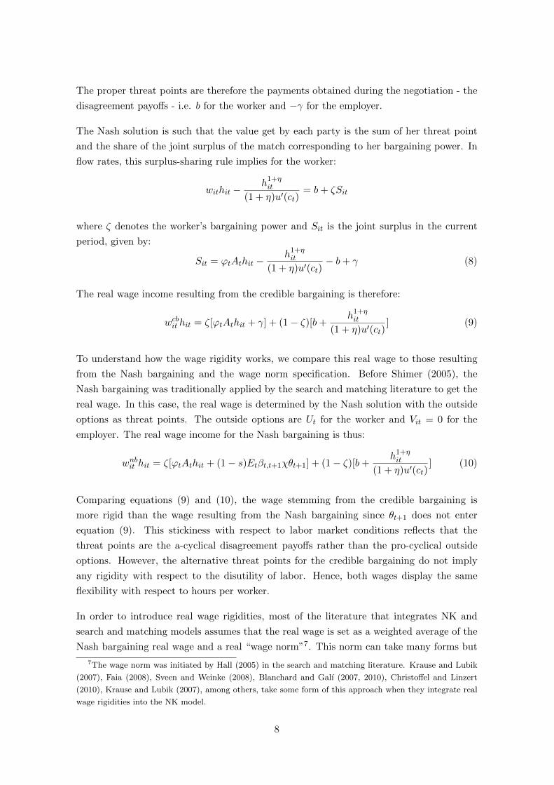
The proper threat points are therefore the payments obtained during the negotiation - the

disagreement payoffs - i.e. b for the worker and −γ for the employer.

The Nash solution is such that the value get by each party is the sum of her threat point

and the share of the joint surplus of the match corresponding to her bargaining power. In

flow rates, this surplus-sharing rule implies for the worker:

withit −h1+ηit

(1 + η)u′(ct)= b+ ζSit

where ζ denotes the worker’s bargaining power and Sit is the joint surplus in the current

period, given by:

Sit = ϕtAthit −h1+ηit

(1 + η)u′(ct)− b+ γ (8)

The real wage income resulting from the credible bargaining is therefore:

wcbit hit = ζ[ϕtAthit + γ] + (1− ζ)[b+h1+ηit

(1 + η)u′(ct)] (9)

To understand how the wage rigidity works, we compare this real wage to those resulting

from the Nash bargaining and the wage norm specification. Before Shimer (2005), the

Nash bargaining was traditionally applied by the search and matching literature to get the

real wage. In this case, the real wage is determined by the Nash solution with the outside

options as threat points. The outside options are Ut for the worker and Vit = 0 for the

employer. The real wage income for the Nash bargaining is thus:

wnbit hit = ζ[ϕtAthit + (1− s)Etβt,t+1χθt+1] + (1− ζ)[b+h1+ηit

(1 + η)u′(ct)] (10)

Comparing equations (9) and (10), the wage stemming from the credible bargaining is

more rigid than the wage resulting from the Nash bargaining since θt+1 does not enter

equation (9). This stickiness with respect to labor market conditions reflects that the

threat points are the a-cyclical disagreement payoffs rather than the pro-cyclical outside

options. However, the alternative threat points for the credible bargaining do not imply

any rigidity with respect to the disutility of labor. Hence, both wages display the same

flexibility with respect to hours per worker.

In order to introduce real wage rigidities, most of the literature that integrates NK and

search and matching models assumes that the real wage is set as a weighted average of the

Nash bargaining real wage and a real “wage norm”7. This norm can take many forms but

7The wage norm was initiated by Hall (2005) in the search and matching literature. Krause and Lubik

(2007), Faia (2008), Sveen and Weinke (2008), Blanchard and Galı (2007, 2010), Christoffel and Linzert

(2010), Krause and Lubik (2007), among others, take some form of this approach when they integrate real

wage rigidities into the NK model.

8

last period’s real wage or a constant real wage are usually considered. Sveen and Weinke

(2008) select a constant wage as a norm. Here, we alternatively retain a backward looking

norm and show that their results carry over. The real hourly wage for the wage norm

specification is therefore:

wwnit = αwwnit−1 + (1− α)wnbit (11)

where α ∈ [0, 1] measures the degree of real wage rigidity. With such a wage rule, the real

wage is sticky not only with respect to labor market conditions but also with respect to

hours per worker.

2.3.3 Hours per worker

The literature has retained two alternative ways of determining hours per worker.

Joint determination of hours per worker A first way assumes that firm and worker

determine hit together in a privately efficient manner, i.e. so as to maximize the joint

surplus of their employment relationship. Maximizing (8) with respect to hit gives the

following first-order condition:

ϕtAt =hηitu′(ct)

(12)

The firm and worker select hit such that the marginal revenue product of labor equals

the worker’s marginal rate of substitution between consumption and leisure. This standard

condition also applies to the Nash bargaining and the wage norm. The consumption/leisure

marginal rate of substitution is the cost of a marginal hour for the firm, whatever the

specification of the wage. Hours are therefore independent of the wage, precisely because

they are chosen to maximize the joint surplus.

Firm’s choice of hours per worker The joint determination of hours has the advantage

of being simple. However, as noticed by Sveen and Weinke (2008), assuming that hours

per worker are determined jointly by the worker and the employer, independently of the

wage, is strong. Trigari (2006) notably argues that hours of work are rarely the object of

bargaining agreements. Therefore a growing part of the recent literature considers that

hours per worker are firm’s choice. Formally, we keep the assumption of Sveen and Weinke

(2008) that hours are chosen by the firm to maximize per-period profit:

Maxhit

[ϕtAthit − withit]

9

which gives the following first order condition:

ϕtAt = w′it(hit)hit + wit (13)

where w′it(hit) is the real marginal hourly wage. Hence, contrary to what happens under

the joint determination of hit, the cost of an additional hour depends on the wage. Using

(9), (10) and (11), the cost of a marginal hour for each wage specification is:

wnbit′(hit)hit + wnbit = ζϕtAt + (1− ζ)

hηitu′(ct)

(14)

wwnit′(hit)hit + wwnit = (1− α)[ζϕtAt + (1− ζ)

hηitu′(ct)

] + αwwnit−1 (15)

wcbit′(hit)hit + wcbit = ζϕtAt + (1− ζ)

hηitu′(ct)

(16)

The cost of a marginal hour is the same under Nash and credible bargainings. At the same

time, since α ∈ [0, 1], the cost of a marginal hour for the wage norm is stickier than for

Nash and credible bargainings.

Comparing both assumptions Finally, let us compare the differences between the two

ways of determining hours. Combining equations (13) with (14) and (13) with (16) gives:

ϕtAt =hηitu′(ct)

which correponds to equation (12). For the Nash and credible bargainings, the cost of a

marginal hour when hours are determined by the firm corresponds to the cost when hours

are determined jointly. This cost is given by the marginal rate of substitution between

consumption and leisure.

Combining equations (13) and (15) gives:

ϕtAt =αwwnit−1 + (1− α)(1− ζ)

hηitu′(ct)

1− (1− α)ζ(17)

Since α ∈ [0, 1], the right-hand side of (17) is less volatile than the marginal rate of substitu-

tion: for the wage norm specification, the cost of a marginal hour when hours are determined

by the firm is stickier than the cost of an additional hour under private efficiency.

10

2.4 Retailers

There is a measure-one continuum of monopolistic retailers, each of them producing one

differentiated consumption good. Cost minimization by households implies that demand

for each retailer j, ydjt, can be written as:

ydjt = (PjtPt

)−εydt (18)

where ydt denotes aggregate demand. I assume that vacancy posting costs take the form of

the same CES function as the one defining the consumption index. Aggregate demand is

therefore given by:

ydt = ct + χvt

The production of ydjt units of good j requires the same amount of the intermediate output,

purchased from producers at the real price ϕt. Thus, ϕt represents the real marginal cost

of production for retailers.

I assume that firms reset their price in a Calvo (1983) fashion. Each period, only a randomly

selected fraction (1− δ) of firms are able to change their price. When a firm has the chance

of reseting its price, it maximizes:

Et

∞∑k=0

δkβt,t+k(PjtPt+k

− ϕt+k)ydjt+k

with respect to Pjt, subject to (18). The optimal price setting rule for a firm resetting its

price in period t is:

Et

∞∑k=0

δkβt,t+kPεt+ky

dt+k(

P ∗tPt+k

− ε

ε− 1ϕt+k) = 0 (19)

where P ∗t is the common price chosen by all price-setters. Hence, price-setters target a

constant mark-up M = εε−1�1 over real marginal costs for the expected duration of the

price set in period t.

We immediately write the optimal price setting condition in a log-linearized form around

a zero-inflation steady-state. Let “hats” denote log-deviations of a variable around its

steady-state value. Equation (19) could be rewritten as:

logP ∗t = (1− βδ)Et∞∑k=0

(βδ)k {ϕt+k + logPt+k} (20)

11

The law of motion for the price level is given by:

P 1−εt = δP 1−ε

t−1 + (1− δ)(P ∗t )1−ε

which has the following log-linear approximation:

logP ∗t − logPt = (δ

1− δ)πt (21)

where πt≡ PtPt−1

is the inflation rate. Combining (20) and (21), we obtain the New-Keynesian

Phillips Curve (NKPC):

πt = βEtπt+1 + κϕt (22)

where κ reads as follows:

κ =(1− δβ)(1− δ)

δ(23)

2.5 Aggregate output and market clearing

Aggregate output yt is obtained by aggregating the final goods of each retailer:

yt≡∫ 1

0[(yjt)

ε−1ε di]

εε−1

The final goods market clearing condition is:

yt = ydt

which implies:

yt = ct + χvt (24)

We also derive the aggregate relation between final and intermediate goods:

xt≡∫ 1

0[xitdi] = yt

∫ 1

0[(PjtPt

)−εdj] (25)

We denote by Dt≡∫ 10 [(

PjtPt

)−εdj] the term capturing the inefficiency resulting from disper-

sion in the quantities consumed of the different final goods, which is itself a consequence

of the price dispersion entailed by staggered price setting. In the neighborhood of the zero

inflation steady state, we have Dt≈1 up to a first order approximation 8. From (27), we

also obtain the approximate aggregate production function:

yt = Atntht (26)

8See Galı (2008, chapters 3 and 4) for details.

12

2.6 Monetary policy

We follow much of the NK literature by assuming that monetary policy is described by a

Taylor interest rate rule:

it = ρiit−1 + (1− ρi)(φππt + φyyt) +mt (27)

where ρi captures the degree of interest rate smoothing, φπ and φy the responses to inflation

and output variations, and mt is an exogenous policy shock that follows an AR(1) process

with autoregressive coefficient ρm and variance σ2m.

3 Positive implication: labor market volatility

3.1 Calibration

From now onwards, we assume the following functional forms for the preferences over con-

sumption and the matching technology:

u(c) =c1−σ

1− σ

m(ut, vt) = m0uςtv

1−ςt

Our model is composed by 9 equations: the employment law of motion (equation (1)), the

Euler equation which describes the evolution of consumption (2), the job creation condition

(7), the real wage (9), the real marginal cost (12), the NKPC (22), the final goods market

clearing condition, the aggregate production function (26) and the Taylor rule (27). The

log-linear equations are listed in the Appendix.

Preferences and price rigidities Time is measured in quarters. We set standard values

for the discount factor β = 0.99 (corresponding to an annual interest rate equal to 4%) as

well as for the intertemporal elasticity of substitution σ = 1. From the estimates of Domeij

and Floden (2006), we set η = 2, corresponding to a standard labor supply elasticity (1/η)

of 0.5.

Following micro evidence, the average duration of a price contract is approximately a year,

which implies δ = 0.75. The elasticity of substitution between differentiated goods ε equals

7.67 (Woodford (2005)).

13

Labor market flows We set the separation rate s to 0.08 (Hall (1995)) and target the

steady state value of the job finding rate to 0.7, which corresponds to monthly rates at less

than 0.03 and 0.3, respectively. We also target the steady state value for the vacancy-to-

unemployment ratio θ to 0.729. The resulting unemployment rate at the steady state is 10%.

This rate is somewhat higher than the observed rate but allows for potential participants

in the matching market such as discouraged workers and workers loosely attached to the

labor force. For the elasticity of the matching function with respect to unemployment, we

select ς = 0.5, in the range of Petrongolo and Pissarides (2001).

Shocks and monetary policy The agregate productivity shock process follows an

AR(1) and based on the RBC literature is calibrated with a standard deviation σa and

an autocorrelation coefficient ρa set to 0.80% and 0.95, respectively10. The monetary pol-

icy is described by a Taylor rule with interest rate smoothing and standard values for the

parameters φπ = 1.5, φy = 0.5/4 and ρ = 0.9. The standard deviation σm of the exogenous

policy shock process is calibrated at 0.132%, to replicate the standard deviation of real

output. While this is not a robust procedure, this is not essential here since the model is

not evaluated along this dimension. The autocorrelation coefficient ρm is set to 0.511.

Wage bargaining parameters and vacancy posting costs The worker’s bargaining

power ζ is chosen at 0.5, a common practice that implies a symmetric bargaining. The flow

value of unemployment b is selected at 0.4, from Shimer (2005). The partial adjustment

coefficient α of the wage norm is set to 0.5, the value commonly used in the literature.

Two parameters remain to calibrate: the cost borne by the employer during the wage

bargaining γ and the vacancy posting cost χ. Since γ is specific to the credible bargaining,

χ is the last parameter to calibrate for the Nash and wage norm specifications. There are

no empirical counterparts for these costs. In order to assign values to those parameters, we

procede in two steps. We begin by determining the value of χ that solves the job-creation

condition at the steady state for the Nash bargaining12. We next replace χ by this value

and find the value of γ that closes the job creation condition at the steady state for the

credible bargaining.

This strategy has two advantages. First, there is a single value for the parameters that

are common to the three wage specifications. Secondly, the real wages at the steady state

under the three specifications are identical13. This last point is critical for the labor market

volatility: as Hagedorn and Manovskii (2008) stress, the labor market is all the more

volatile as the steady state profit is low (and therefore as the steady state real wage is

9The sample mean for θ in 1960-2006 (Pissarides (2009)).10See Faia (2008, 2009) for details.11This value is also retained by Galı (2008, 2010).12The resulting value for χ is also the value that solves the job creation condition under the wage norm,

since at the steady state the real wages for the Nash bargaining and the wage norm are identical.13Since the resulting value for γ equals (1 − s)βχθ.

14

high). By implying identical real wages at the steady state, our calibration does not favour

any particular specification.

The value of χ that closes the job creation condition at the steady state for the Nash

solution is 0.23. Given this value for χ, the job creation condition at the steady state under

the credible bargaining is solved for γ = 0.15. All the parameters are summarized in the

following table.

Parameter Definition Value

β Discount factor 0.99

σ Intertemporal elasticity of substitution 1

η Convexity of labor disutility 2

δ Fraction of unchanged prices 0.75

ε Elasticity of demand curves 7.67

s Separation rate 0.08

ς Elasticity matching fct wrt vacancies 0.5

σa SD of productivity shock 0.80%

ρa AC of productivity shock 0.95

σm SD of policy shock 0.132%

ρm AC of policy shock 0.5

φπ Response to inflation in the Taylor rule 1.5

φy Response to output gap in the Taylor rule 0.5/4

ρ Interest rate smoothing 0.9

ζ Worker’s bargaining power 0.5

b Flow value of unemployment 0.4

χ Vacancy posting cost 0.23

γ Employer’s cost of delay 0.15

3.2 Labor market volatility

Tables 1 and 2 display the standard deviations of the main labor market variables for

the three wage specifications. Those tables provide the results when the source of the

fluctuations are productivity shocks (“Prod.”), monetary policy shocks (“Mon.”) and both

types of shocks together.

15

Tab

le1:

Lab

or

mark

et

vola

tility

/C

red

ible

an

dN

ash

barg

ain

ings

Cre

dib

leB

arg

ain

ing

Nash

Barg

ain

ing

Std

Devia

tion

sD

ata

aP

rod

.M

on

.B

oth

Pro

d.

Mon

.B

oth

Ou

tpu

t0.0

160.

009

0.01

30.

016

0.00

70.

012

0.01

4

Un

emp

loym

ent

6.9

04.

305.

615.

232.

703.

633.

43

Vac

an

cies

8.2

55.

568.

287.

514.

035.

415.

10

Tig

htn

ess

14.9

59.

8013

.70

12.5

86.

638.

928.

39

Hou

rsp

erw

orke

r0.3

50.

620.

400.

480.

690.

600.

63

Rea

lw

age

0.70

0.77

1.04

0.96

1.20

1.78

1.66

aSta

tist

ics

for

the

US

econom

yare

com

pute

dusi

ng

quart

erly

(wit

ha

smooth

ing

para

met

erof

1600)

HP

-filt

ered

data

from

1964:1

to2002:3

.T

he

standard

dev

iati

ons

of

all

wari

able

sare

rela

tive

tooutp

ut.

16

Tab

le2:

Lab

or

mark

et

vola

tility

/W

age

norm

Dete

rmin

ati

on

ofhit

by

firm

sJoin

td

ete

rmin

ati

on

ofhit

Std

Devia

tion

sD

ata

Pro

d.

Mon

.B

oth

Pro

d.

Mon

.B

oth

Ou

tpu

t0.0

16

0.00

80.

014

0.01

60.

008

0.01

30.

015

Un

emp

loym

ent

6.90

1.93

2.83

2.63

3.12

4.92

4.51

Vaca

nci

es8.2

52.

804.

143.

844.

937.

807.

19

Tig

htn

ess

14.9

54.

676.

866.

387.

8612

.47

11.4

8

Hou

rsp

erw

ork

er0.

350.

720.

690.

700.

630.

450.

51

Rea

lw

age

0.70

0.69

0.83

0.79

0.80

1.05

1.01

17

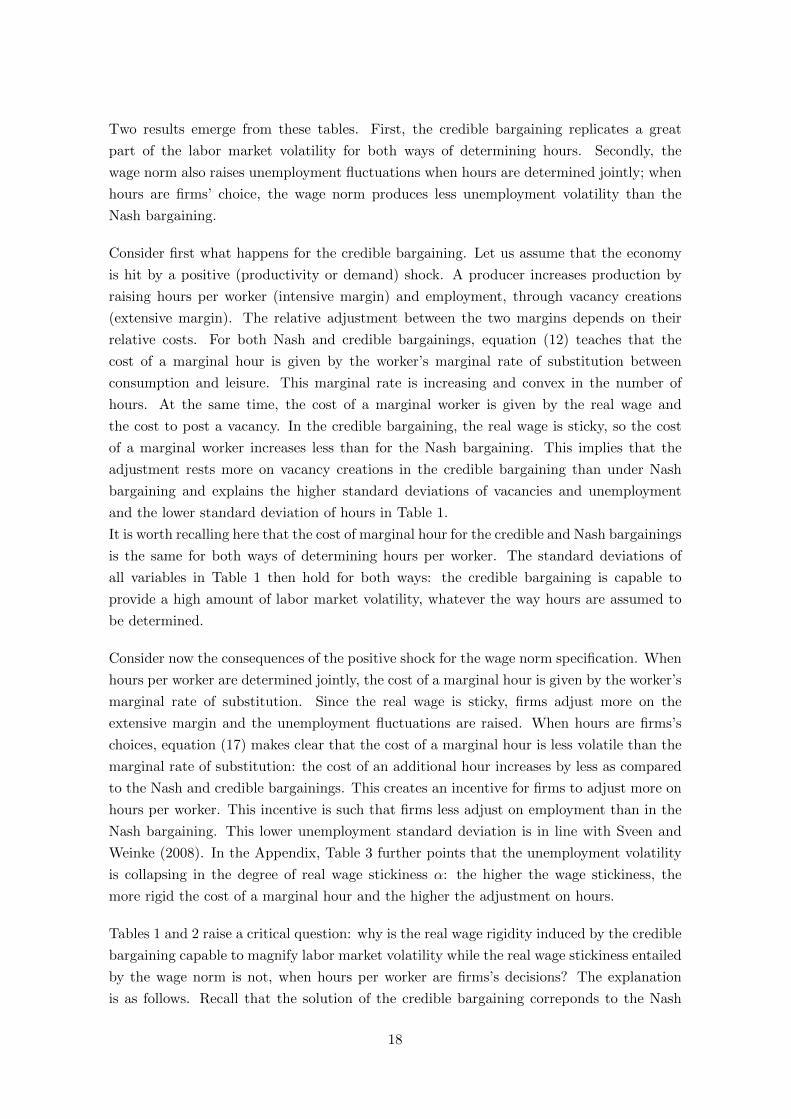
Two results emerge from these tables. First, the credible bargaining replicates a great

part of the labor market volatility for both ways of determining hours. Secondly, the

wage norm also raises unemployment fluctuations when hours are determined jointly; when

hours are firms’ choice, the wage norm produces less unemployment volatility than the

Nash bargaining.

Consider first what happens for the credible bargaining. Let us assume that the economy

is hit by a positive (productivity or demand) shock. A producer increases production by

raising hours per worker (intensive margin) and employment, through vacancy creations

(extensive margin). The relative adjustment between the two margins depends on their

relative costs. For both Nash and credible bargainings, equation (12) teaches that the

cost of a marginal hour is given by the worker’s marginal rate of substitution between

consumption and leisure. This marginal rate is increasing and convex in the number of

hours. At the same time, the cost of a marginal worker is given by the real wage and

the cost to post a vacancy. In the credible bargaining, the real wage is sticky, so the cost

of a marginal worker increases less than for the Nash bargaining. This implies that the

adjustment rests more on vacancy creations in the credible bargaining than under Nash

bargaining and explains the higher standard deviations of vacancies and unemployment

and the lower standard deviation of hours in Table 1.

It is worth recalling here that the cost of marginal hour for the credible and Nash bargainings

is the same for both ways of determining hours per worker. The standard deviations of

all variables in Table 1 then hold for both ways: the credible bargaining is capable to

provide a high amount of labor market volatility, whatever the way hours are assumed to

be determined.

Consider now the consequences of the positive shock for the wage norm specification. When

hours per worker are determined jointly, the cost of a marginal hour is given by the worker’s

marginal rate of substitution. Since the real wage is sticky, firms adjust more on the

extensive margin and the unemployment fluctuations are raised. When hours are firms’s

choices, equation (17) makes clear that the cost of a marginal hour is less volatile than the

marginal rate of substitution: the cost of an additional hour increases by less as compared

to the Nash and credible bargainings. This creates an incentive for firms to adjust more on

hours per worker. This incentive is such that firms less adjust on employment than in the

Nash bargaining. This lower unemployment standard deviation is in line with Sveen and

Weinke (2008). In the Appendix, Table 3 further points that the unemployment volatility

is collapsing in the degree of real wage stickiness α: the higher the wage stickiness, the

more rigid the cost of a marginal hour and the higher the adjustment on hours.

Tables 1 and 2 raise a critical question: why is the real wage rigidity induced by the credible

bargaining capable to magnify labor market volatility while the real wage stickiness entailed

by the wage norm is not, when hours per worker are firms’s decisions? The explanation

is as follows. Recall that the solution of the credible bargaining correponds to the Nash

18

solution with the credible threat points. On a frictional labor market, those threat points

are no longer the outside options, which depend on labor market conditions, but rather the

a-cyclical disagreement payoffs. The real wage resulting from the credible bargaining is thus

sticky with respect to labor market fluctuations. Nevertheless, the a-cyclical threat points

of the credible bargaining do not deliver any wage stickiness with respect to the disutility

of work and then with respect to hours per worker: as for the Nash bargaining, the cost

of marginal hour is equal to the worker’s marginal rate of substitution, which is increasing

and convex in the number of hours. With a real wage rigid with respect to labor market

conditions but flexible with respect to hours per worker, firms adjust less on hours and

more on vacancies. Instead, the wage norm specification sets the real wage as a weighted

average of the Nash bargaining wage and the last’s period wage. Consequently, the real

wage is sticky with respect to both labor market fluctuations and hours per worker. The

rigidity of the wage with respect to hours encourages firms to adjust more on hours per

worker.

Sveen and Weinke (2008) introduce real wage rigidities through the wage norm specification

and conclude that the capacity of those rigidities to solve the puzzle raised by Shimer (2005)

critically depends on the way hours per worker are chosen. Their unability to magnify

unemployment fluctuations when hours are firms’s choices would imply that real wage

rigidities are not the answer to this puzzle. From Table 1, we instead argue that what is

critical is the way that rigidities are introduced. Once real wage rigidities result from the

credible bargaining, they considerably enhance labor market volatility, whatever the way

hours are determined. Real wage rigidities are therefore the required ingredient to solve

the puzzle.

Finally, another interesting feature of the credible bargaining is related to the degree of

wage stickiness. From Table 1, the relative standard deviation of the real wage to the real

output is slightly higher than what is observed empirically. The credible bargaining then

avoids the usual criticism which states that models with real wage rigidities generate a real

wage sharply more sticky than in the data. This criticism is relevant for standard search and

matching models, which are purely real and allow no adjustment on the intensive margin.

In that models, the only variable component of the real wage is the labor productivity,

itself weakly volatile. In our monetary model with adjustment on the intensive margin, the

real marginal cost and hours per worker are other variables that enter the wage equation.

The resulting real wage is stickier than Nash bargaining wage but displays slightly more

volatility than in the data.

19

4 Normative implication: an inflation/unemployment stabi-

lization trade-off

Blanchard and Galı (2007, 2010) argue that for the canonical NK model, in which the real

wage is flexible, the strict inflation targeting policy is efficient. Indeed, they demonstrate

that a full stabilization of the inflation rate implies that the fluctuations of the unemploy-

ment rate mimic those of the constrained-efficient allocation, which would be the allocation

chosen by a benevolent planner. This absence of a stabilization trade-off between inflation

and unemployment, at odds with conventional wisdom, is what Blanchard and Galı call the

divine coincidence. Nevertheless, when real wage rigidities are introduced, the unemploy-

ment fluctuations resulting from the zero inflation policy are much more volatile than that

of the constrained-efficient rate: with real wage stickiness, strict inflation targeting entails

inefficient fluctuations of the unemployment rate and the central bank faces a stabilization

trade-off.

In this section, I point that when firms can adjust on the intensive margin, the capacity

of real wage rigidities for providing a policy trade-off critically depends on the way those

rigidities are introduced. I find that for the credible bargaining, strict inflation target-

ing produces inefficient unemployment variations whatever the determination of hours per

worker while for the wage norm specification, inefficient unemployment movements appear

only for hours determined jointly.

4.1 The constrained-efficient allocation

The social planner chooses the state-contingent path of ct, ht, vt and nt that maximizes

the joint welfare of households and managers:

∞∑t=0

βt

{u(ct)− nt

h1+ηt

1 + η

}

subject to the aggregate resource constraint:

Atntht + b(1− nt) = ct + χvt (28)

and the law of motion of employment:

nt = (1− s)nt−1 + q(θt)vt (29)

20

Since the benevolent planner avoids any inefficient dispersion in relative prices, the price

dispersion term Dt equals 1. Using (28) to substitute for ct in the objective function, the

social planner is left with the choice of ht, vt and nt. The first-order condition with respect

to ht is given by:

At =hηt

u′(ct)(30)

From (30), the social planner equalizes the marginal product of labor and the marginal

rate of substitution between consumption and leisure. Merging first order conditions with

respect to nt and vt delivers the job creation condition for the constrained-efficient alloca-

tion:

χ

q(θt)= (1− ς)[Atht − b−

h1+ηt

(1 + η)u′(ct)] + (1− s)Etβt,t+1[−ςχθt+1 +

χ

q(θt+1)] (31)

In the equilibrium allocation of the decentralized economy, when the real wage is determined

by the Nash bargaining, the first-order condition with respect to hit was instead given by

equation (12) (whatever the way hours per worker are chosen):

Atϕt =hηt

u′(ct)

The job creation condition for this decentralized allocation is obtained by substituting (10)

into (7). This gives:

χ

q(θt)= (1− ζ)[ϕtAtht − b−

h1+ηt

(1 + η)u′(ct)] + (1− s)Etβt,t+1[−ζχθt+1 +

χ

q(θt+1)] (32)

The correspondence between equations (30) and (12) on one side, and equations (31) and

(32) on the other, is ensured under the three following conditions:

ς = ζ (i)

ϕ = 1 (ii)

ϕt = 1 ∀t (iii)

Condition (i) is the well-known Hosios (1990) condition stating that the efficient number

of vacancy creations is such that the bargaining power of workers ζ equals their share in

the matching technology ς. Vacancy posting decisions generate a negative externality in

the form of vacancy posting costs that reduce the resources available for consumption. The

costs to post vacancies are increasing in ς. The higher these costs, the lower the efficient

number of vacancy creations. An higher ζ is therefore required since the implied higher

wage induces fewer vacancy openings.

21

Condition (ii) deals with the goods market and requires the absence of a market power for

final goods firms. Recall that ϕ is the real marginal cost for retailers, which is inversely

related to their mark-up. The usual way to eliminate this mark-up is to assume that

retailers sales are subsidized (through lump-sum taxes) at the rate 1ε−1 .

Conditions (i) and (ii) imply an efficient steady state.

Condition (iii) states that the real marginal cost should be stabilized at one in every period.

From the NKPC, stabilizing ϕt corresponds to a full stabilization of the price level: a strict

inflation targeting policy implements the constrained-efficient allocation.

Hence, for an efficient steady state, the zero inflation policy is optimal when the real wage

is Nash-bargained. This is the point raised by Blanchard and Galı (2007): when real

wages are flexible, there is divine coincidence between stabilizing inflation and stabilizing

unemployment around its rate at the first best.

4.2 Strict inflation targeting and inefficient unemployment fluctuations

In what follows, we assume that the steady state is efficient. We thus set ζ = ς and ϕ = 1.

Nevertheless, for the credible bargaining, there is an additional condition required to ensure

the efficiency of the steady state. The job creation condition under this wage bargaining is:

χ

q(θt)= (1− ζ)[ϕtAtht − b− (1− ζ)

h1+ηt

(1 + η)u′(ct)]− ζγ + (1− s)βt,t+1Et

χ

q(θt+1)

Evaluated at the steady state and setting ζ = ς and ϕ = 1, this equation becomes:

χ

q(θ)(1− β(1− s)) = (1− ς)[Ah− b− (1− ς) h1+η

(1 + η)u′(c)]− ςγ (33)

At the steady state, the efficient job creation condition (equation (31)) is given by:

χ

q(θ)(1− β(1− s)) = (1− ς)[Ah− b− (1− ς) h1+η

(1 + η)u′(c)]− β(1− s)ςχθ (34)

Equation (33) corresponds to (34) for γ = (1 − s)βχθ. This condition provides a positive

relation between the employer’s cost borne during the wage bargaining γ and the vacancy

posting costs χθ. The explanation is the same as the one given for the Hosios condition: the

higher the costs to post vacancies, the higher is the γ consistent with the efficient allocation

since the resulting higher wage (see equation (9)) entails fewer vacancy creations.

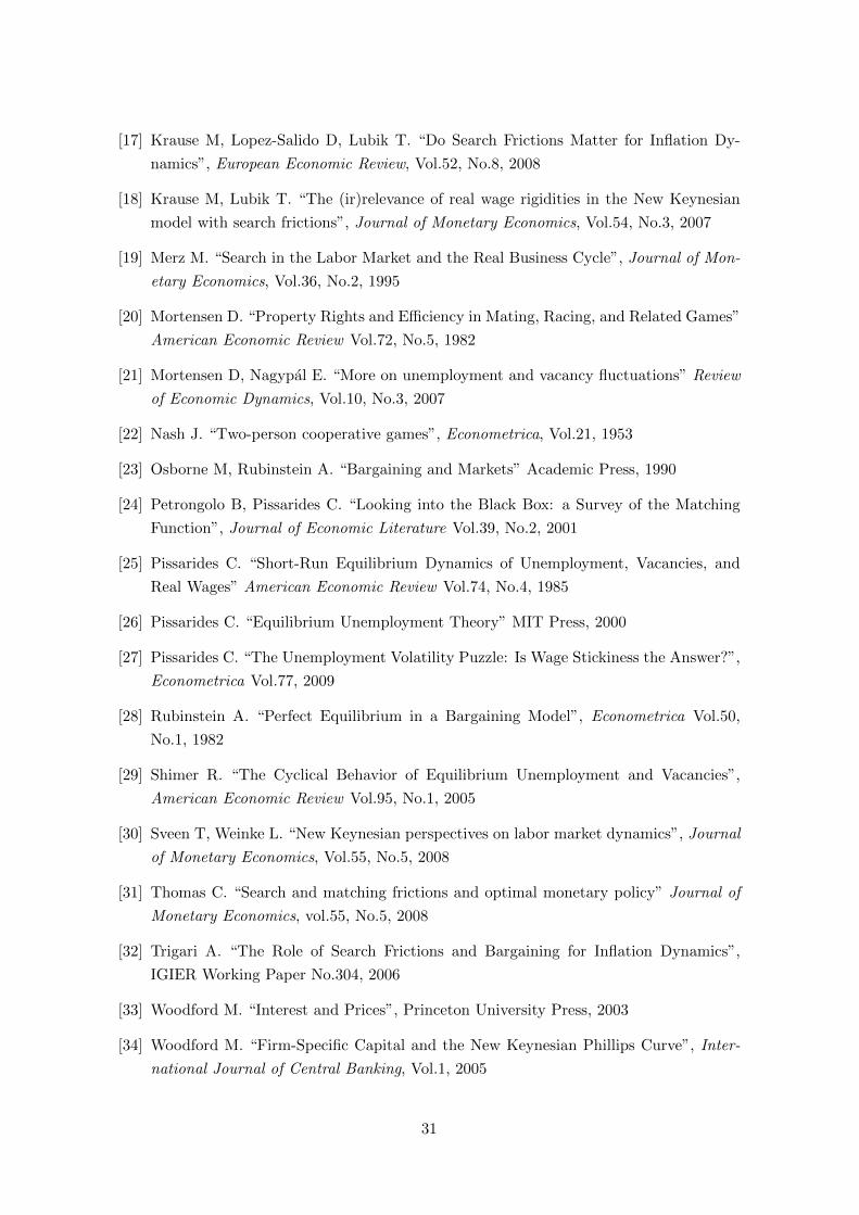
The plain lines in Figure 1 display the efficient responses of the unemployment rate and

hours per worker to a 1% negative productivity shock. The dashed lines represent the

22

responses of that variables under the strict inflation targeting policy, i.e. the policy that

keeps the price level constant in every period. This policy is implemented by fully stabilizing

the real marginal cost each period. All the responses are shown in percentage points.

23

Figure 1: impulse responses to a 1% negative productivity shock

Credible Bargaining

Unemployment Hours per worker

Wage Norm / joint determination of hours

Unemployment Hours per worker

Wage Norm / hours determined by firms

Unemployment Hours per worker

0 5 10 15 20 25 30 35 400

1

2

3

4

5

6

7

8

0 5 10 15 20 25 30 35 400

1

2

3

4

5

6

7

8

0 5 10 15 20 25 30 35 400

1

2

3

4

5

6

7

8

0 5 10 15 20 25 30 35 40

-0,6

-0,4

-0,2

0

0,2

0,4

0,6

0 5 10 15 20 25 30 35 40

-0,6

-0,4

-0,2

0

0,2

0,4

0,6

0 5 10 15 20 25 30 35 40

-0,6

-0,4

-0,2

0

0,2

0,4

0,6

24

For the credible bargaining, the unemployment rate under strict inflation targeting is much

more volatile than the efficient rate: the zero inflation policy entails large and inefficient

unemployment fluctuations. At the same time, hours per worker are hardly more respon-

sive under strict inflation targeting than the first best. The real wage stickiness resulting

from the credible bargaining therefore creates a meaningful stabilization trade-off between

inflation and unemployment, whatever the determination of hours per worker.

The results for the wage norm specification are still dependent on the way hours are chosen.

When hours are determined jointly, the dynamics of unemployment and hours resemble to

the credible bargaining. In this case, the real wage rigidities induced by the wage norm

break the divine coincidence. Conversely, when hours are firms’ choice, the movements in

unemployment are weak and close to the efficient rate while hours per worker display much

larger variations. In this case, the real wage rigidities implied by the wage norm generate

a stabilization trade-off between inflation and hours per worker, but no longer between

inflation and unemployment.

Why does the real wage rigidity provided by the credible bargaining deliver an infla-

tion/unemployment trade-off while the wage stickiness resulting from the wage norm does

not, when hours are firms’ decisions? Recall that for the credible bargaining, the real wage

is sticky with respect to labor market conditions but flexible with respect to disutility of

work. As a result, the cost of a marginal hour is very flexible and makes firms less adjust

on the intensive margin and more on employment. The unemployment rate thus displays

larger fluctuations than the rate resulting from the Nash bargaining, which corresponds to

the efficient rate under zero inflation policy.

For the wage norm specification, the real wage is sticky with respect to both labor market

conditions and disutility of work. As we have pointed in the positive analysis, the resulting

stickiness in the cost of an additional hour creates an incentive for firms to adjust more on

hours per worker. This explains the higher response of hours while unemployment does not

exhibit larger variations than the efficient rate.

This unability of the wage norm to provide a stabilization trade-off contrats with the result

of Blanchard and Galı (2007, 2010) who introduce real wage rigidities through the lens of a

wage norm. However, their analysis is led in a model in which labor supply is inelastic. In

such a framework, firms can only adjust on employment and the wage stickiness resulting

from the wage norm generates inefficient variations of the unemployment rate.

The failure of the wage norm to bring an inflation/unemployment stabilization trade-off

when hours are determined through firms’ profit maximization could challenge the role

of real wage rigidities in generating such a trade-off, as Sveen and Weinke (2008) did for

the labor market volatility. We again argue that the way of introducing wage rigidities is

critical. Since for the credible bargaining zero inflation policies produce large and inefficient

unemployment fluctuations, whatever the way hours are determined, real wage rigidities

are the required ingredient to produce a meaningful policy trade-off.

25

5 Conclusion

Sveen and Weinke (2008) have argued that the ability of real wage rigidities to amplify labor

market volatility crucially depends on the way hours per workers are determined. In this

paper, we have pointed out that what is critical is instead the way those rigidities are intro-

duced. We have replaced the traditional ad-hoc wage norm by the credible bargaining into a

NK model with search frictions. We have shown that the resulting micro-founded real wage

rigidities raise unemployment fluctuations and provide a significant inflation/unemployment

stabilization trade-off, whatever the way hours are determined. Since the real wage is sticky

with respect to labor market conditions but flexible with respect to disutility of work, firms

adjust more and employment and less on the intensive margin. Conversely, for the wage

norm specification, the real wage is sticky with respect to both labor market conditions and

disutility of work. This creates an incentive for firms to adjust more on hours per worker

and less on employment.

26

Appendix: log-linearized equilibrium conditions

We restrict attention to a log-linear approximation to the equilibrium dynamics around a

zero inflation steady state. A variable without a time subscript denotes the steady state

value of that variable while hats are meant to indicate log-deviations of a variable around

its steady state value.

Tightness:

θt = vt − ut

Employment law of motion:

nt = (1− s)nt−1 +m0uςv1−ς(ςut + (1− ς)vt)

Unemployment:

ut = −nunt

Euler equation:

ct = Etct+1 − (it − Etπt+1)

Aggregate production function:

yt = At + ht + nt

Final goods market clearing condition:

yt =c

yct +

χv

yvt

NKPC:

πt = βEtπt+1 + κϕt

Real marginal cost:

ϕt = ηht + ct − At

27

Job-creation condition:

χ

q(θ)ςθt = ϕAh|ϕt + At + ht]− wh[wt + ht] + (1− s)βEt[

χ

q(θ)ςθt+1 + ct − ct+1]

Real hourly wage:

wt =

{ζϕA[ϕt + At]− ζγht − (1− ζ)bht +

1− ζ1 + η

c[ηht + ct]}1

w

28

Tab

le3:

Lab

or

mark

et

vola

tility

/W

age

norm

-d

ete

rmin

ati

on

of

hou

rsby

firm

s

Std

Devia

tion

sD

ata

WN

WN

WN

WN

(α=

0.2)

(α=

0.4)

(α=

0.6)

(α=

0.8)

Ou

tpu

t0.

016

0.01

50.

015

0.01

70.

019

Un

emp

loym

ent

6.9

03.

142.

812.

401.

82

Vaca

nci

es8.2

54.

684.

163.

502.

53

Tig

htn

ess

14.9

57.

726.

875.

834.

29

Hou

rsp

erw

ork

er0.

350.

650.

690.

720.

77

Rea

lw

age

0.7

01.

280.

950.

640.

32

29

References

[1] Benigno P, Woodford M. “Inflation Stabilization And Welfare: The Case Of A Dis-

torted Steady State” Journal of the European Economic Association, MIT Press, vol.3,

No.6, 2005

[2] Binmore K, Rubinstein A, Wolinsky A. “The Nash bargaining solution in economic

modelling”, Rand Journal of Economics Vol.17, No.2, 1986

[3] Blanchard O, Galı J. “Real Wage Rigidities and the New Keynesian Model” Journal

of Money, Credit and Banking, supplement to Vol.39, No.1, 2007

[4] Blanchard O, Galı J. “Labor markets and Monetary Policy: A New Keynesian Model

with Unemployment”, American Economic Review: Macroeconomics Vol.2, No.2, 2010

[5] Calvo G. “Staggered Prices in a Utility-Maximizing Framework”, Journal of Monetary

Economics, Vol.12, 1983

[6] Christoffel K, Kuester K. “Resuscitating the Wage Channel in Models with Unemploy-

ment Fluctuations”, Journal of Monetary Economics Vol.55, No.5, 2008

[7] Christoffel K, Linzert T. “The Role of Real Wage Rigidity and Labor Market Rigidities

in Inflation Persistence”, Journal of Money, Credit and Banking Vol.42, No.7, 2010

[8] Domeij D, Floden M. “The labor-supply elasticity and borrowing constraints: why

estimates are biased”, Review of Economic Dynamics Vol.9, No.2, 2006

[9] Faia E. “Optimal Monetary Policy Rules with Labour Market Frictions”, Journal of

Economic Dynamics and Control, Vol.32(5), 2008

[10] Faia E. “Ramsey Monetary Policy with Labour Market frictions”, Journal of Monetary

Economics, Vol.56, No.4, 2009

[11] Galı J. “Monetary Policy, Inflation, and the Business Cycle”, Princeton University

Press, 2008

[12] Galı J. “Monetary Policy and Unemployment”, Handbook of Monetary Economics,

2010

[13] Hagedorn M, Manovskii I. “The Cyclical Behavior of Equilibrium Unemployment and

Vacancies Revisited”, American Economic Review Vol.98, No.4, 2008

[14] Hall R. “Lost Jobs”, Brookings Papers on Economic Activity, Vol.1, 1995

[15] Hall R. “Employment Fluctuations with Equilibrium Wage Stickiness” American Eco-

nomic Review Vol.95, No.1, 2005

[16] Hall R, Milgrom P. “The limited Influence of Unemployment on the Wage Bargain”,

American Economic Review Vol.98, No.4, 2008

30

[17] Krause M, Lopez-Salido D, Lubik T. “Do Search Frictions Matter for Inflation Dy-

namics”, European Economic Review, Vol.52, No.8, 2008

[18] Krause M, Lubik T. “The (ir)relevance of real wage rigidities in the New Keynesian

model with search frictions”, Journal of Monetary Economics, Vol.54, No.3, 2007

[19] Merz M. “Search in the Labor Market and the Real Business Cycle”, Journal of Mon-

etary Economics, Vol.36, No.2, 1995

[20] Mortensen D. “Property Rights and Efficiency in Mating, Racing, and Related Games”

American Economic Review Vol.72, No.5, 1982

[21] Mortensen D, Nagypal E. “More on unemployment and vacancy fluctuations” Review

of Economic Dynamics, Vol.10, No.3, 2007

[22] Nash J. “Two-person cooperative games”, Econometrica, Vol.21, 1953

[23] Osborne M, Rubinstein A. “Bargaining and Markets” Academic Press, 1990

[24] Petrongolo B, Pissarides C. “Looking into the Black Box: a Survey of the Matching

Function”, Journal of Economic Literature Vol.39, No.2, 2001

[25] Pissarides C. “Short-Run Equilibrium Dynamics of Unemployment, Vacancies, and

Real Wages” American Economic Review Vol.74, No.4, 1985

[26] Pissarides C. “Equilibrium Unemployment Theory” MIT Press, 2000

[27] Pissarides C. “The Unemployment Volatility Puzzle: Is Wage Stickiness the Answer?”,

Econometrica Vol.77, 2009

[28] Rubinstein A. “Perfect Equilibrium in a Bargaining Model”, Econometrica Vol.50,

No.1, 1982

[29] Shimer R. “The Cyclical Behavior of Equilibrium Unemployment and Vacancies”,

American Economic Review Vol.95, No.1, 2005

[30] Sveen T, Weinke L. “New Keynesian perspectives on labor market dynamics”, Journal

of Monetary Economics, Vol.55, No.5, 2008

[31] Thomas C. “Search and matching frictions and optimal monetary policy” Journal of

Monetary Economics, vol.55, No.5, 2008

[32] Trigari A. “The Role of Search Frictions and Bargaining for Inflation Dynamics”,

IGIER Working Paper No.304, 2006

[33] Woodford M. “Interest and Prices”, Princeton University Press, 2003

[34] Woodford M. “Firm-Specific Capital and the New Keynesian Phillips Curve”, Inter-

national Journal of Central Banking, Vol.1, 2005

31