a new finite element gradient recovery method ...zzhang/paper/zhang-naga1.pdf · a new finite...

A New Finite Element Gradient Recovery Method:

Superconvergence Property

Zhimin Zhang∗†and Ahmed Naga ‡

Department of Mathematics, Wayne State University, Detroit, MI 48202

Abstract

This is the first in a series of papers where a new gradient recovery method is introduced and analyzed. Itis proved that the method is superconvergent for translation invariant finite element spaces of any order.The method maintains the simplicity, efficiency, and superconvergence properties of the Zienkiewicz-Zhupatch recovery method. In addition, under uniform triangular meshes, the method is superconvergent forthe Chevron pattern, and ultraconvergent at element edge centers for the regular pattern. Applicationsof this new gradient recovery technique will be discussed in forthcoming papers.

Key Words. finite element method, least-squares fitting, ZZ patch recovery, superconvergence,ultraconvergence

AMS Subject Classification. 65N30, 65N15, 65N12, 65D10, 74S05, 41A10, 41A25

1 Introduction

A decade has passed since the first appearance of the Zienkiewicz-Zhu gradient patch recovery

method [23] based on a local discrete least-squares fittings. The method is now widely used

in engineering practices for its robustness in a posteriori error estimates and its efficiency in

computer implementation. It is a common belief that the robustness of the ZZ patch recovery

is rooted in its superconvergence property under structured meshes. Even for an unstructured

mesh, when adaptive is used, a mesh refinement will usually bring in some kind of structure

locally. Superconvergence properties of the ZZ patch recovery are proved in [21] for all popular

elements under rectangular mesh and in [10] for the linear element under strongly regular

triangular meshes. A closer look reveals that the ZZ patch recovery is not superconvergent for

linear element under uniform triangular mesh of the Chevron pattern, nor it is superconvergent

for quadratic element at edge centers under uniform triangular mesh of the regular pattern

(see Section 4). This observation is confirmed by numerical tests (see Section 5). The question

naturally arises: Can we find a better recovery method? The new method should keep all

advantageous properties of the ZZ patch recovery while improving it under other situations,

e.g., the two cases we mentioned above.

∗This research was partially supported by the National Science Foundation grants DMS-0074301, DMS-

0079743, and DMS-0311807.†E-mail: [email protected]‡E-mail: [email protected]

1

In this paper, we introduce and analyze such a new gradient recovery method. Given a finite

element space of degree k, instead of fitting (in a least-squares sense) a polynomial of degree k

to gradient values at some sampling points on element patches (as in the ZZ patch recovery),

the new method fits a polynomial of degree k + 1 to solution values at some nodal points, and

then takes derivatives to obtain recovered gradient at each assembly points. The idea is also

related to the meshless method [12] where we only pay attention to nearby surrounding nodes

and not to elements. We shall prove that the new method is superconvergent for translation

invariant finite element spaces of any order. We shall also demonstrate that the new method

processes all known superconvergence and “ultraconvergence” (superconvergence with order

2) properties of the ZZ method, and is applicable to arbitrary grids with cost comparable to

the ZZ patch recovery. In computer implementation, there is no significant difference between

least-squares fitting a polynomial of degree k or degree k + 1, compared with the overall cost

in finite element solution.

The idea of fitting solution values was investigated earlier in [19] to recover finite element

solutions and to obtain the L2 norm a posteriori error estimates. Recently, Wang [18] proposed a

semi-local L2-projection (continuous least-squares fitting) to smooth the finite element solution.

Here we use the fitted solution values to recover the gradient and further to construct a posteriori

error estimates in the energy norm. Furthermore, there is no need for element patches in our

approach, and the method is “meshless”.

The application of the new recovery method to a posteriori error estimates and its compari-

son with the ZZ estimator will be discussed in a forthcoming paper, in which we shall utilize an

integral identity developed recently in [4] to prove the asymptotic exactness of the a posteriori

error estimator based on the new recovery method under arbitrary grid. In this respect, the

reader is also referred to a recent book by Ainsworth and Oden [1] for discussion of recovery

type a posteriori error estimators.

2 Meshless gradient recovery method

We introduce a new gradient recovery operator Gh : Sh → Sh × Sh, where Sh is a polynomial

finite element space of degree k over a triangulation Th. Given a finite element solution uh, we

need to define Ghuh at the following three types of nodes: vertices, edge nodes, and internal

nodes. For the linear element all nodes are vertices, for the quadratic element there are vertices

and edge-center nodes, and for the cubic element all three types of nodes are presented. After

determining values of Ghuh at all nodes, we obtain Ghuh ∈ Sh × Sh on the whole domain by

interpolation using the original nodal shape functions of Sh.

1) We start from vertices. For a vertex zzzi, let hi be the length of the longest edge attached

to zzzi. we select all nodes on the ball

Bhi(zzzi) = zzz ∈ D : |zzz − zzzi| ≤ hi,

where D is the solution domain. If the number of nodes n (including zzzi) is less than m =

(k + 2)(k + 3)/2, we go further and include nodes in B2hi(zzzi), continuing this process until we

have a sufficient number of nodes. We then denote them as zzzij , and fit a polynomial of degree

k + 1, in the least-squares sense, to the finite element solution uh at those nodes. Using the

2

local coordinates (x, y) with zzzi as the origin, the fitting polynomial is

pk+1(x, y;zzzi) = PPP Taaa = PPPTaaa,

with

PPP T = (1, x, y, x2, · · · , xk+1, xky, · · · , yk+1), PPPT

= (1, ξ, η, ξ2, · · · , ξk+1, ξkη, · · · , ηk+1);

aaaT = (a1, a2, · · · , am), aaaT = (a1, ha2, · · · , hk+1am),

where the scaling parameter h = hi. The coefficient vector aaa is determined by the linear system

AT Aaaa = ATbbbh, (2.1)

where bbbTh = (uh(zzzi1), uh(zzzi2), · · · , uh(zzzin)) and

A =

1 ξ1 η1 · · · ηk+11

1 ξ2 η2 · · · ηk+12

1 ξ3 η3 · · · ηk+13

......

......

...1 ξn ηn · · · ηk+1

n

.

The condition for (2.1) to have a unique solution is

RankA = m, (2.2)

which is almost always satisfied in practical situation when n ≥ m and grid points are reasonably

distributed. Now we define

Ghuh(zzzi) = ∇pk+1(0, 0;zzzi). (2.3)

2) If zzzi is an edge node which lies on an edge between two vertices zzzi1 and zzzi2 , we define

Ghuh(zzzi) = α∇pk+1(x1, y1;zzzi1) + (1 − α)∇pk+1(x2, y2;zzzi2), 0 < α < 1, (2.4)

where (x1, y1) (or (x2, y2)) is the local coordinates of zzzi with origin at zzzi1 (or zzzi2). The weight

α is determined by the ratio of the distances of zzzi to zzzi1 and zzzi2 .

3) If zzzi is an internal node which lies in a triangle formed by three vertices zzzi1 , zzzi2 , and zzzi3 ,

we define

Ghuh(zzzi) =3

∑

j=1

αj∇pk+1(xj , yj ;zzzij ),3

∑

j=1

αj = 1, αj > 0, (2.5)

where (xj , yj) is the local coordinates of zzzi with origin at zzzij . The weight αj is determined by

the ratio of the distances of zzzi to zzzi1 , zzzi2 , and zzzi3 .

In order to demonstrate the method, we shall discuss two examples in details. For the

sake of simplicity and superconvergence analysis, both examples are under uniform meshes.

Nevertheless, the method can be applied to arbitrary meshes even with curved boundaries, see

Fig. 15.

3

Example 1. Linear element on uniform triangular mesh. First, we consider the regular pattern

(Fig. 1). We fit a quadratic polynomial

p2(ξ, η) = (1, ξ, η, ξ2, ξη, η2)(a1, · · · , a6)T

in a least-squares sense with respect to the seven nodal values in (ξ, η) coordinates

~ξ = (0, 1, 0,−1,−1, 0, 1)T , ~η = (0, 0, 1, 1, 0,−1,−1)T .

Denote ~e = (1, 1, 1, 1, 1, 1, 1)T and set

A = (~e, ~ξ, ~η, ~ξ2, ~ξη, ~η2),

with ~ξ2 = (ξ21 , ξ

22 , · · · , ξ2

7)T , and ~ξη, ~η2 defined accordingly. We calculate

(AT A)−1AT =1

6

6 0 0 0 0 0 00 2 1 −1 −2 −1 10 1 2 1 −1 −2 −1−6 3 0 0 3 0 0−6 3 3 −3 3 3 −3−6 0 3 0 0 3 0

,

and obtain p2 from aaa = (AT A)−1ATbbb. In order to investigate the approximation property of

the recovery operator, we let bbbT = (u0, u1, . . . , u6) instead of using the finite element solution

uh. Recall

(a1, a2, a3, a4, a5, a6) = (a1, ha2, ha3, h2a4, h

2a5, h2a6),

and we obtain

p2(x, y) = u0 +1

6h[2(u1 − u4) + u2 − u3 + u6 − u5]x

+1

6h[2(u2 − u5) + u1 − u6 + u3 − u4]y +

1

2h2(u1 − 2u0 + u4)x

2

+1

2h2(u1 − 2u0 + u4 + u2 − u3 + u5 − u6)xy +

1

2h2(u2 − 2u0 + u5)y

2.

We see that

∂p2

∂x(x, y) =

1

6h[2(u1 − u4) + u2 − u3 + u6 − u5]

+1

h2(u1 − 2u0 + u4)x +

1

2h2(u1 − 2u0 + u4 + u2 − u3 + u5 − u6)y; (2.6)

∂p2

∂y(x, y) =

1

6h[2(u2 − u5) + u1 − u6 + u3 − u4]

+1

2h2(u1 − 2u0 + u4 + u2 − u3 + u5 − u6)x +

1

h2(u2 − 2u0 + u5)y. (2.7)

By the Taylor expansion, it is straight forward to verify that (2.6) and (2.7) provide a second

order approximation to ∇u, especially at (x, y) = (0, 0) where we have a finite difference scheme

1

6h

(

2(u1 − u4) + u2 − u3 + u6 − u5

2(u2 − u5) + u3 − u4 + u1 − u6

)

. (2.8)

4

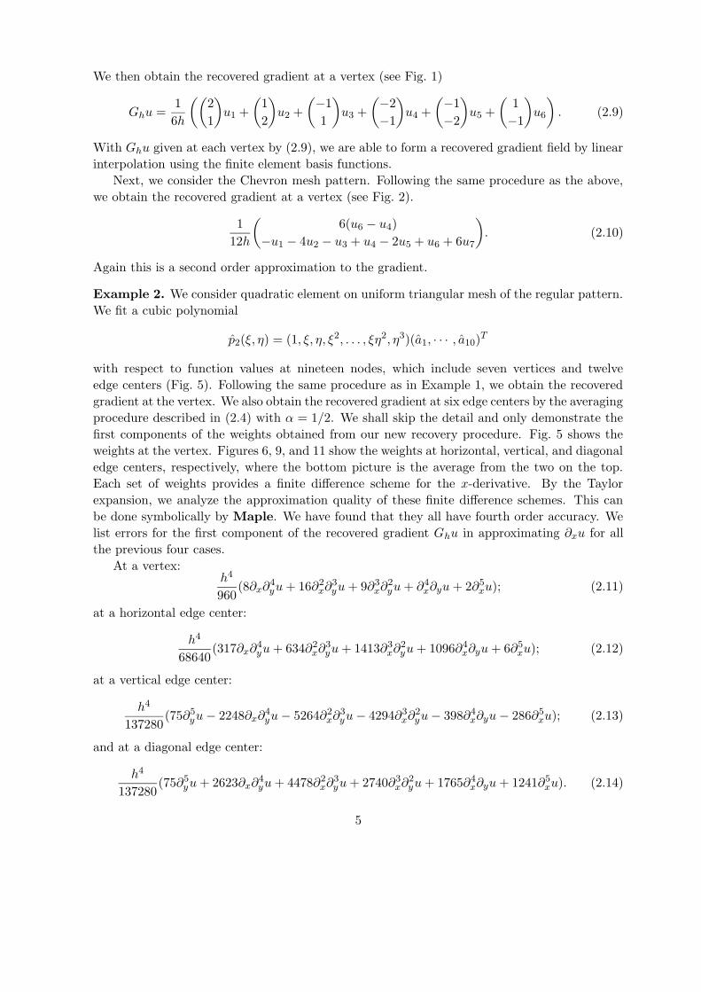
We then obtain the recovered gradient at a vertex (see Fig. 1)

Ghu =1

6h

((

2

1

)

u1 +

(

1

2

)

u2 +

(

−1

1

)

u3 +

(

−2

−1

)

u4 +

(

−1

−2

)

u5 +

(

1

−1

)

u6

)

. (2.9)

With Ghu given at each vertex by (2.9), we are able to form a recovered gradient field by linear

interpolation using the finite element basis functions.

Next, we consider the Chevron mesh pattern. Following the same procedure as the above,

we obtain the recovered gradient at a vertex (see Fig. 2).

1

12h

(

6(u6 − u4)

−u1 − 4u2 − u3 + u4 − 2u5 + u6 + 6u7

)

. (2.10)

Again this is a second order approximation to the gradient.

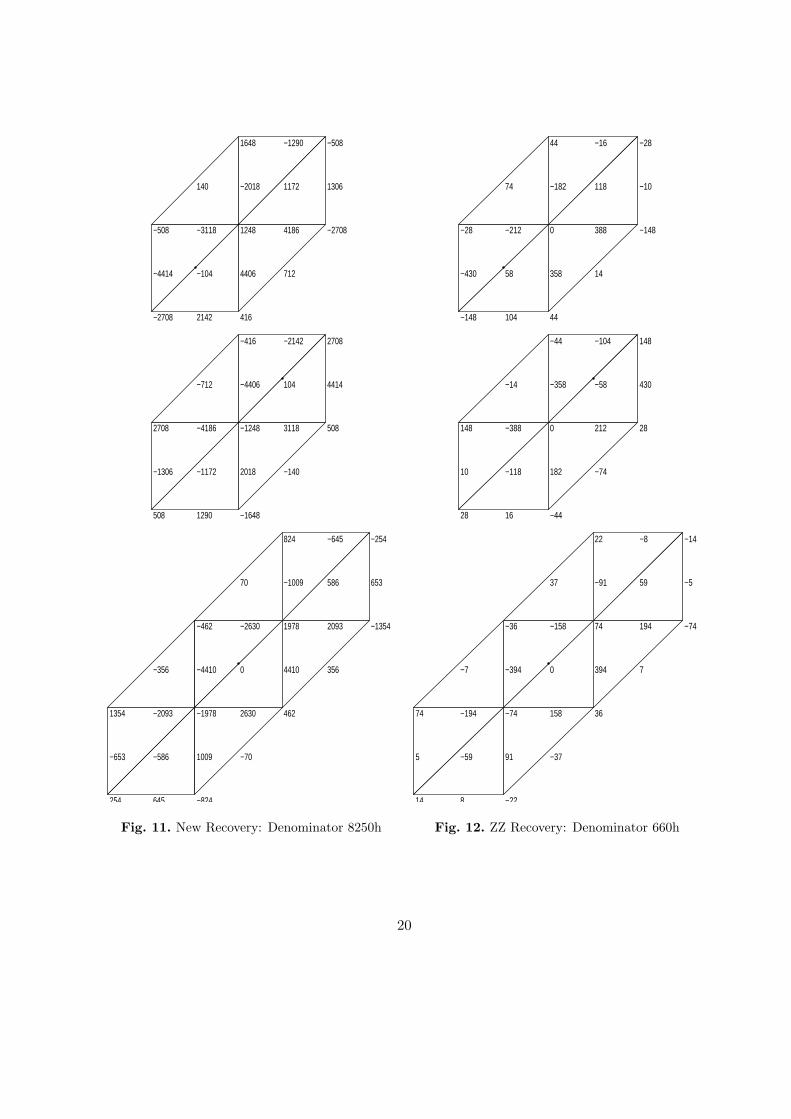
Example 2. We consider quadratic element on uniform triangular mesh of the regular pattern.

We fit a cubic polynomial

p2(ξ, η) = (1, ξ, η, ξ2, . . . , ξη2, η3)(a1, · · · , a10)T

with respect to function values at nineteen nodes, which include seven vertices and twelve

edge centers (Fig. 5). Following the same procedure as in Example 1, we obtain the recovered

gradient at the vertex. We also obtain the recovered gradient at six edge centers by the averaging

procedure described in (2.4) with α = 1/2. We shall skip the detail and only demonstrate the

first components of the weights obtained from our new recovery procedure. Fig. 5 shows the

weights at the vertex. Figures 6, 9, and 11 show the weights at horizontal, vertical, and diagonal

edge centers, respectively, where the bottom picture is the average from the two on the top.

Each set of weights provides a finite difference scheme for the x-derivative. By the Taylor

expansion, we analyze the approximation quality of these finite difference schemes. This can

be done symbolically by Maple. We have found that they all have fourth order accuracy. We

list errors for the first component of the recovered gradient Ghu in approximating ∂xu for all

the previous four cases.

At a vertex:h4

960(8∂x∂4

yu + 16∂2x∂3

yu + 9∂3x∂2

yu + ∂4x∂yu + 2∂5

xu); (2.11)

at a horizontal edge center:

h4

68640(317∂x∂4

yu + 634∂2x∂3

yu + 1413∂3x∂2

yu + 1096∂4x∂yu + 6∂5

xu); (2.12)

at a vertical edge center:

h4

137280(75∂5

yu − 2248∂x∂4yu − 5264∂2

x∂3yu − 4294∂3

x∂2yu − 398∂4

x∂yu − 286∂5xu); (2.13)

and at a diagonal edge center:

h4

137280(75∂5

yu + 2623∂x∂4yu + 4478∂2

x∂3yu + 2740∂3

x∂2yu + 1765∂4

x∂yu + 1241∂5xu). (2.14)

5

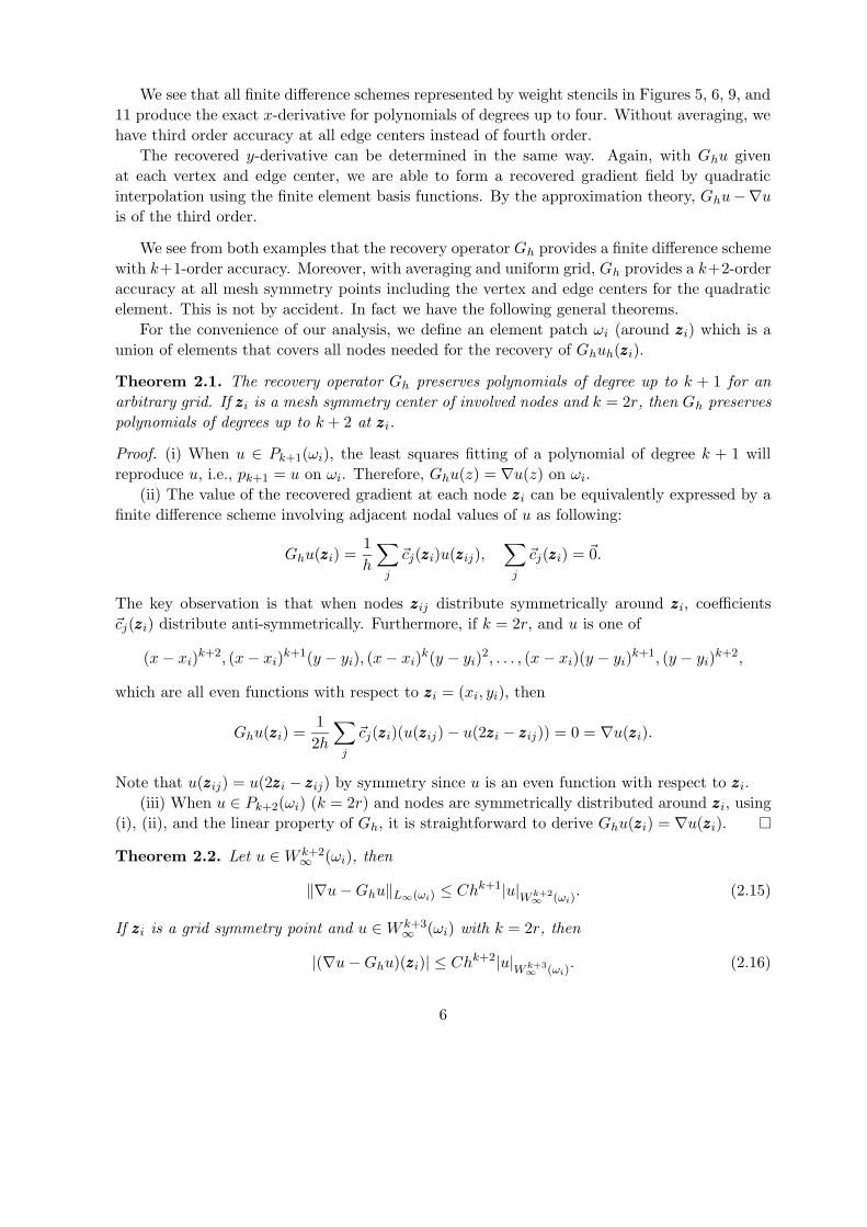
We see that all finite difference schemes represented by weight stencils in Figures 5, 6, 9, and

11 produce the exact x-derivative for polynomials of degrees up to four. Without averaging, we

have third order accuracy at all edge centers instead of fourth order.

The recovered y-derivative can be determined in the same way. Again, with Ghu given

at each vertex and edge center, we are able to form a recovered gradient field by quadratic

interpolation using the finite element basis functions. By the approximation theory, Ghu−∇u

is of the third order.

We see from both examples that the recovery operator Gh provides a finite difference scheme

with k+1-order accuracy. Moreover, with averaging and uniform grid, Gh provides a k+2-order

accuracy at all mesh symmetry points including the vertex and edge centers for the quadratic

element. This is not by accident. In fact we have the following general theorems.

For the convenience of our analysis, we define an element patch ωi (around zzzi) which is a

union of elements that covers all nodes needed for the recovery of Ghuh(zzzi).

Theorem 2.1. The recovery operator Gh preserves polynomials of degree up to k + 1 for an

arbitrary grid. If zzzi is a mesh symmetry center of involved nodes and k = 2r, then Gh preserves

polynomials of degrees up to k + 2 at zzzi.

Proof. (i) When u ∈ Pk+1(ωi), the least squares fitting of a polynomial of degree k + 1 will

reproduce u, i.e., pk+1 = u on ωi. Therefore, Ghu(z) = ∇u(z) on ωi.

(ii) The value of the recovered gradient at each node zzzi can be equivalently expressed by a

finite difference scheme involving adjacent nodal values of u as following:

Ghu(zzzi) =1

h

∑

j

~cj(zzzi)u(zzzij),∑

j

~cj(zzzi) = ~0.

The key observation is that when nodes zzzij distribute symmetrically around zzzi, coefficients

~cj(zzzi) distribute anti-symmetrically. Furthermore, if k = 2r, and u is one of

(x − xi)k+2, (x − xi)

k+1(y − yi), (x − xi)k(y − yi)

2, . . . , (x − xi)(y − yi)k+1, (y − yi)

k+2,

which are all even functions with respect to zzzi = (xi, yi), then

Ghu(zzzi) =1

2h

∑

j

~cj(zzzi)(u(zzzij) − u(2zzzi − zzzij)) = 0 = ∇u(zzzi).

Note that u(zzzij) = u(2zzzi − zzzij) by symmetry since u is an even function with respect to zzzi.

(iii) When u ∈ Pk+2(ωi) (k = 2r) and nodes are symmetrically distributed around zzzi, using

(i), (ii), and the linear property of Gh, it is straightforward to derive Ghu(zzzi) = ∇u(zzzi).

Theorem 2.2. Let u ∈ W k+2∞ (ωi), then

‖∇u − Ghu‖L∞(ωi) ≤ Chk+1|u|W k+2∞ (ωi)

. (2.15)

If zzzi is a grid symmetry point and u ∈ W k+3∞ (ωi) with k = 2r, then

|(∇u − Ghu)(zzzi)| ≤ Chk+2|u|W k+3∞ (ωi)

. (2.16)

6

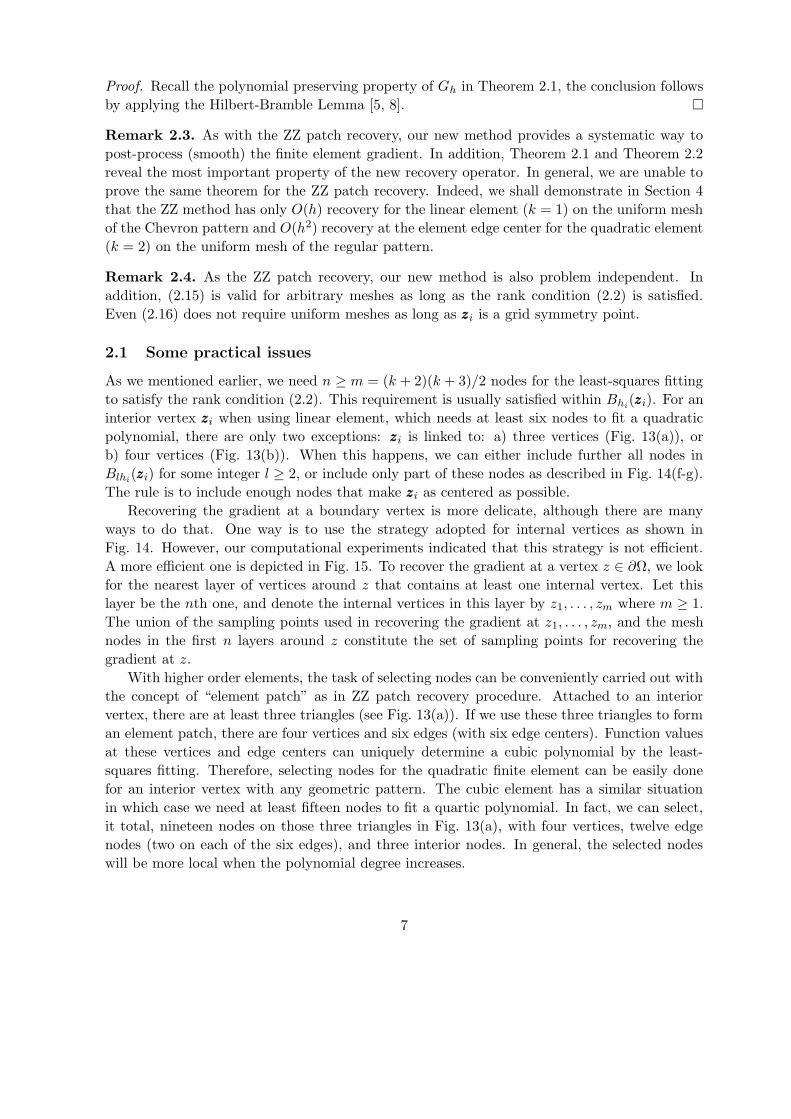
Proof. Recall the polynomial preserving property of Gh in Theorem 2.1, the conclusion follows

by applying the Hilbert-Bramble Lemma [5, 8].

Remark 2.3. As with the ZZ patch recovery, our new method provides a systematic way to

post-process (smooth) the finite element gradient. In addition, Theorem 2.1 and Theorem 2.2

reveal the most important property of the new recovery operator. In general, we are unable to

prove the same theorem for the ZZ patch recovery. Indeed, we shall demonstrate in Section 4

that the ZZ method has only O(h) recovery for the linear element (k = 1) on the uniform mesh

of the Chevron pattern and O(h2) recovery at the element edge center for the quadratic element

(k = 2) on the uniform mesh of the regular pattern.

Remark 2.4. As the ZZ patch recovery, our new method is also problem independent. In

addition, (2.15) is valid for arbitrary meshes as long as the rank condition (2.2) is satisfied.

Even (2.16) does not require uniform meshes as long as zzzi is a grid symmetry point.

2.1 Some practical issues

As we mentioned earlier, we need n ≥ m = (k + 2)(k + 3)/2 nodes for the least-squares fitting

to satisfy the rank condition (2.2). This requirement is usually satisfied within Bhi(zzzi). For an

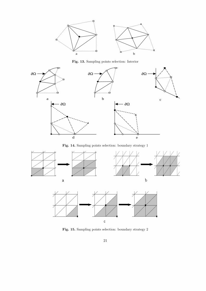
interior vertex zzzi when using linear element, which needs at least six nodes to fit a quadratic

polynomial, there are only two exceptions: zzzi is linked to: a) three vertices (Fig. 13(a)), or

b) four vertices (Fig. 13(b)). When this happens, we can either include further all nodes in

Blhi(zzzi) for some integer l ≥ 2, or include only part of these nodes as described in Fig. 14(f-g).

The rule is to include enough nodes that make zzzi as centered as possible.

Recovering the gradient at a boundary vertex is more delicate, although there are many

ways to do that. One way is to use the strategy adopted for internal vertices as shown in

Fig. 14. However, our computational experiments indicated that this strategy is not efficient.

A more efficient one is depicted in Fig. 15. To recover the gradient at a vertex z ∈ ∂Ω, we look

for the nearest layer of vertices around z that contains at least one internal vertex. Let this

layer be the nth one, and denote the internal vertices in this layer by z1, . . . , zm where m ≥ 1.

The union of the sampling points used in recovering the gradient at z1, . . . , zm, and the mesh

nodes in the first n layers around z constitute the set of sampling points for recovering the

gradient at z.

With higher order elements, the task of selecting nodes can be conveniently carried out with

the concept of “element patch” as in ZZ patch recovery procedure. Attached to an interior

vertex, there are at least three triangles (see Fig. 13(a)). If we use these three triangles to form

an element patch, there are four vertices and six edges (with six edge centers). Function values

at these vertices and edge centers can uniquely determine a cubic polynomial by the least-

squares fitting. Therefore, selecting nodes for the quadratic finite element can be easily done

for an interior vertex with any geometric pattern. The cubic element has a similar situation

in which case we need at least fifteen nodes to fit a quartic polynomial. In fact, we can select,

it total, nineteen nodes on those three triangles in Fig. 13(a), with four vertices, twelve edge

nodes (two on each of the six edges), and three interior nodes. In general, the selected nodes

will be more local when the polynomial degree increases.

7

3 Superconvergence analysis

In this section, we utilize a tool in [14, 15, 17] to prove the superconvergence property of our

recovery operator. We refer readers to [5, 8] for general theory of the finite element method

and to [7, 9, 11, 17, 22] for the superconvergence theory.

First, we observe that the recovery operator results in a difference quotient. Let us take

linear element on uniform triangular mesh of the regular pattern as an example. The recovered

derivative at a nodal point O is (see Fig. 1)

∂hxu(O) =

1

6h[u2 − u3 + 2(u1 − u4) + u6 − u5].

Let φj be the nodal shape functions. Then we can express

∂hxu(O)φ0(x, y)

=1

6h[u2φ2(x, y + h) − u3φ3(x − h, y + h) + 2u1φ1(x + h, y)

− 2u4φ4(x − h, y) + u6φ6(x + h, y − h) − u5φ5(x, y − h)].

We see that the translations are in the directions of l1 = ±(1, 0), l2 = ±(0, 1), and l3 = ±(1,−1).

Therefore, we can express the recovered x-derivative as

∂hxuh(zzz) =

∑

|ν|≤M

3∑

i=1

C(i)ν,huh(zzz + νhli). (3.1)

The analysis here follows closely the argument of Wahlbin in [17, §8.2]. We consider the

finite element approximation of the solution of a scalar second order elliptic problem. With

D ⊂⊂ R2 a basic domain, Sh ⊂ H1(D) a parameterized family of finite element spaces, Ω ⊂⊂ D

and S0h(Ω) = v ∈ Sh : suppv ⊂ Ω, let u and uh ∈ Sh be two functions such that

A(u − uh, v) = 0, ∀v ∈ S0h(Ω),

where

A(w, v) =

∫ 2∑

i,j=1

aij∂w

∂xi

∂v

∂xj+

2∑

i=1

bi∂w

∂xiv + cwv.

Let Ω0 ⊂⊂ Ω1 ⊂⊂ Ω be separated by d ≥ c0h, let ` be a unit vector in R2, and let H be a

parameter, which is a constant times h. Denote by T `H , a translation by H in the direction `,

i.e., T `Hv(zzz) = v(zzz + H`), and for ν an integer,

T `νHv(zzz) = v(zzz + νH`) (3.2)

Then the finite element space is called translation invariant by H in the direction ` if

T `νHv ∈ S0

h(Ω), ∀v ∈ S0h(Ω1), |ν| ≤ M

for a fixed M . For constant coefficients A, we have

A(T `νH(u − uh), v) = A(u − uh, T `

−νHv) = A(u − uh, (T `νH)∗v) = 0, ∀v ∈ S0

h(Ω1).

8

Consequently, for Gh, a difference operator constructed from translations of type (3.2), we have

A(Gh(u − uh), vvv) = A(u − uh, G∗hvvv) = 0, ∀vvv ∈ S0

h(Ω1)2.

Therefore, from Theorem 5.5.2 of [17] (with F ≡ 0), we have

‖Gh(u − uh)‖L∞(Ω0) ≤ C(lnd

h)r min

vvv∈Sh×Sh

‖Ghu − vvv‖L∞(Ω1) (3.3)

+Cd−s−2/q‖Gh(u − uh)‖W−sq (Ω1)

. (3.4)

Here r = 1 for linear element and r = 0 for higher order elements. The first term on the right

hand side of (3.3) can be estimated by the standard approximation theory under the assumption

that the finite element space includes piecewise polynomials of degree k.

‖Ghu − vvv‖L∞(Ω1) ≤ Chk+1|u|W k+2∞ (Ω1). (3.5)

For the second term, we have

‖Gh(u − uh)‖W−sq (Ω1) = sup

φφφ∈C∞0 (Ω1)2,‖φφφ‖Ws

q′(Ω1)=1

(Gh(u − uh),φφφ).

Here

(Gh(u − uh),φφφ) = (u − uh, G∗hφφφ)

≤ C1‖u − uh‖L∞(Ω1+Mh)‖G∗hφφφ‖L1(Ω1+Mh)

≤ C2‖u − uh‖L∞(Ω1+Mh), (3.6)

where Ω1 + Mh define a sub-domain that stretches out Mh from Ω1. Note that when s ≥ 1,

‖G∗hφφφ‖L1(Ω1+Mh) is bounded uniformly with respect to h. Applying Theorem 5.5.2 in [17] again,

we have

‖u − uh‖L∞(Ω1+Mh) ≤ C(lnd

h)r min

v∈Sh

‖u − v‖L∞(Ω) + Cd−s−2/q‖u − uh‖W−sq (Ω)

≤ C(lnd

h)rhk+1‖u‖W k+1

∞ (Ω) + Cd−s−2/q‖u − uh‖W−sq (Ω). (3.7)

If the separation parameter d = O(1), then combining (3.3) to (3.7), we have shown:

‖Gh(u − uh)‖L∞(Ω0) ≤ C(ln1

h)rhk+1‖u‖W k+2

∞ (Ω) + C‖u − uh‖W−sq (Ω) (3.8)

Now we are ready for the main theorem of the paper.

Theorem 3.1. Let the coefficients in differential operator A be constants, let the finite element

space, which includes piecewise polynomials of degree k, be translation invariant in directions

required by the recovery operator Gh on Ω ⊂⊂ D, and let u ∈ W k+2∞ (Ω). Assume that A(u −

uh, v) = 0 for v ∈ S0h(Ω). Assume further that Theorem 5.5.2 in [17] is applicable. Then on

any interior region Ω0 ⊂⊂ Ω, there is a constant C independent of h and u such that

‖∇u − Ghuh‖L∞(Ω0) ≤ C(ln1

h)rhk+1‖u‖W k+2

∞ (Ω) + C‖u − uh‖W−sq (D), (3.9)

for some s ≥ 0 and q ≥ 1.

9

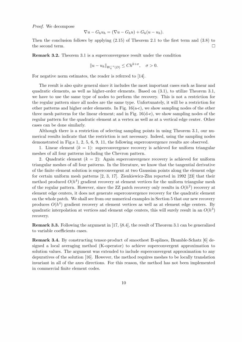
Proof. We decompose

∇u − Ghuh = (∇u − Ghu) + Gh(u − uh).

Then the conclusion follows by applying (2.15) of Theorem 2.1 to the first term and (3.8) to

the second term.

Remark 3.2. Theorem 3.1 is a superconvergence result under the condition

‖u − uh‖W−sq (D) ≤ Chk+σ, σ > 0.

For negative norm estimates, the reader is referred to [14].

The result is also quite general since it includes the most important cases such as linear and

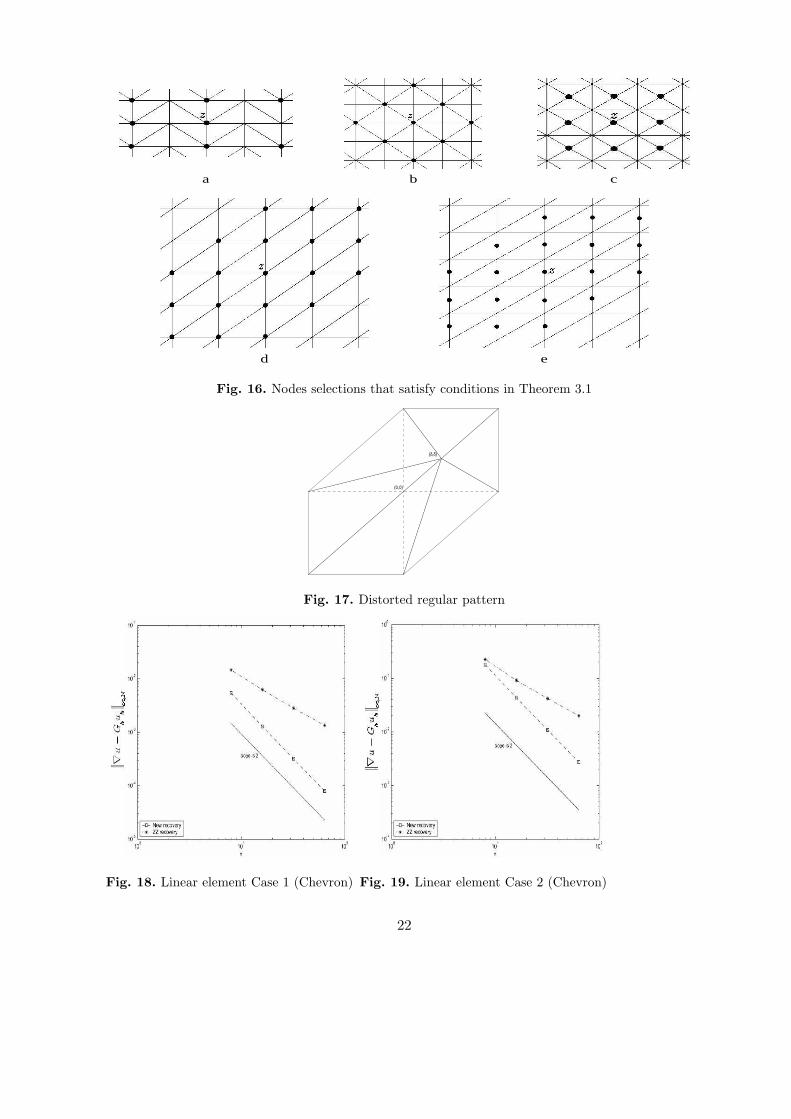
quadratic elements, as well as higher-order elements. Based on (3.1), to utilize Theorem 3.1,

we have to use the same type of nodes to perform the recovery. This is not a restriction for

the regular pattern since all nodes are the same type. Unfortunately, it will be a restriction for

other patterns and higher order elements. In Fig. 16(a-c), we show sampling nodes of the other

three mesh patterns for the linear element; and in Fig. 16(d-e), we show sampling nodes of the

regular pattern for the quadratic element at a vertex as well as at a vertical edge center. Other

cases can be done similarly.

Although there is a restriction of selecting sampling points in using Theorem 3.1, our nu-

merical results indicate that the restriction is not necessary. Indeed, using the sampling nodes

demonstrated in Fig.s 1, 2, 5, 6, 9, 11, the following superconvergence results are observed.

1. Linear element (k = 1): superconvergence recovery is achieved for uniform triangular

meshes of all four patterns including the Chevron pattern.

2. Quadratic element (k = 2): Again superconvergence recovery is achieved for uniform

triangular meshes of all four patterns. In the literature, we know that the tangential derivative

of the finite element solution is superconvergent at two Gaussian points along the element edge

for certain uniform mesh patterns [2, 3, 17]. Zienkiewicz-Zhu reported in 1992 [23] that their

method produced O(h4) gradient recovery at element vertices for the uniform triangular mesh

of the regular pattern. However, since the ZZ patch recovery only results in O(h2) recovery at

element edge centers, it does not generate superconvergence recovery for the quadratic element

on the whole patch. We shall see from our numerical examples in Section 5 that our new recovery

produces O(h4) gradient recovery at element vertices as well as at element edge centers. By

quadratic interpolation at vertices and element edge centers, this will surely result in an O(h3)

recovery.

Remark 3.3. Following the argument in [17, §8.4], the result of Theorem 3.1 can be generalized

to variable coefficients cases.

Remark 3.4. By constructing tensor-product of smoothest B-splines, Bramble-Schatz [6] de-

signed a local averaging method (K-operator) to achieve superconvergent approximation to

solution values. The argument was extended to include superconvergent approximation to any

depuratives of the solution [16]. However, the method requires meshes to be locally translation

invariant in all of the axes directions. For this reason, the method has not been implemented

in commercial finite element codes.

10

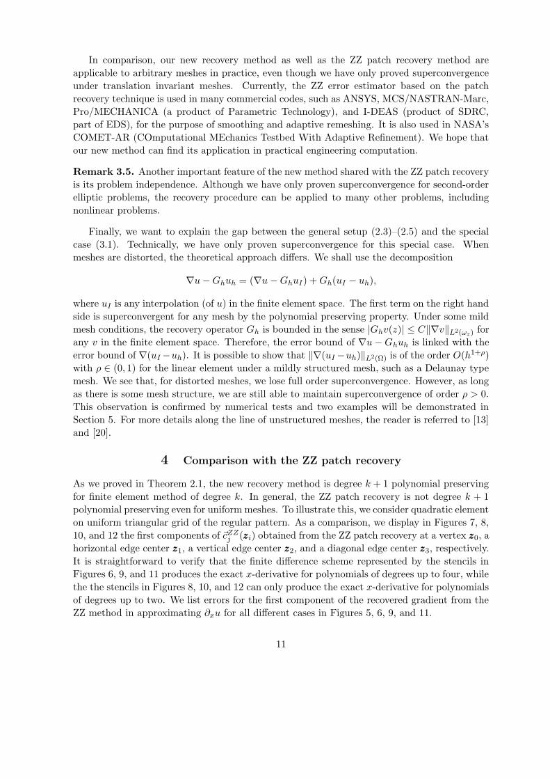
In comparison, our new recovery method as well as the ZZ patch recovery method are

applicable to arbitrary meshes in practice, even though we have only proved superconvergence

under translation invariant meshes. Currently, the ZZ error estimator based on the patch

recovery technique is used in many commercial codes, such as ANSYS, MCS/NASTRAN-Marc,

Pro/MECHANICA (a product of Parametric Technology), and I-DEAS (product of SDRC,

part of EDS), for the purpose of smoothing and adaptive remeshing. It is also used in NASA’s

COMET-AR (COmputational MEchanics Testbed With Adaptive Refinement). We hope that

our new method can find its application in practical engineering computation.

Remark 3.5. Another important feature of the new method shared with the ZZ patch recovery

is its problem independence. Although we have only proven superconvergence for second-order

elliptic problems, the recovery procedure can be applied to many other problems, including

nonlinear problems.

Finally, we want to explain the gap between the general setup (2.3)–(2.5) and the special

case (3.1). Technically, we have only proven superconvergence for this special case. When

meshes are distorted, the theoretical approach differs. We shall use the decomposition

∇u − Ghuh = (∇u − GhuI) + Gh(uI − uh),

where uI is any interpolation (of u) in the finite element space. The first term on the right hand

side is superconvergent for any mesh by the polynomial preserving property. Under some mild

mesh conditions, the recovery operator Gh is bounded in the sense |Ghv(z)| ≤ C‖∇v‖L2(ωz) for

any v in the finite element space. Therefore, the error bound of ∇u − Ghuh is linked with the

error bound of ∇(uI −uh). It is possible to show that ‖∇(uI −uh)‖L2(Ω) is of the order O(h1+ρ)

with ρ ∈ (0, 1) for the linear element under a mildly structured mesh, such as a Delaunay type

mesh. We see that, for distorted meshes, we lose full order superconvergence. However, as long

as there is some mesh structure, we are still able to maintain superconvergence of order ρ > 0.

This observation is confirmed by numerical tests and two examples will be demonstrated in

Section 5. For more details along the line of unstructured meshes, the reader is referred to [13]

and [20].

4 Comparison with the ZZ patch recovery

As we proved in Theorem 2.1, the new recovery method is degree k + 1 polynomial preserving

for finite element method of degree k. In general, the ZZ patch recovery is not degree k + 1

polynomial preserving even for uniform meshes. To illustrate this, we consider quadratic element

on uniform triangular grid of the regular pattern. As a comparison, we display in Figures 7, 8,

10, and 12 the first components of ~cZZj (zzzi) obtained from the ZZ patch recovery at a vertex zzz0, a

horizontal edge center zzz1, a vertical edge center zzz2, and a diagonal edge center zzz3, respectively.

It is straightforward to verify that the finite difference scheme represented by the stencils in

Figures 6, 9, and 11 produces the exact x-derivative for polynomials of degrees up to four, while

the the stencils in Figures 8, 10, and 12 can only produce the exact x-derivative for polynomials

of degrees up to two. We list errors for the first component of the recovered gradient from the

ZZ method in approximating ∂xu for all different cases in Figures 5, 6, 9, and 11.

11

At a vertex:

h4

1920(10∂x∂4

yu + 20∂2x∂3

yu + 15∂3x∂2

yu + 5∂4x∂yu + 4∂5

xu); (4.1)

at a horizontal edge center:h2

264∂3

xu; (4.2)

at a vertical edge center:h2

264(3∂2

x∂yu + 2∂3xu); (4.3)

at a diagonal edge center:h2

264(3∂2

x∂yu + ∂3xu). (4.4)

We see that only second order accuracy is achieved at all edge centers even with averaging.

On an irregular grid, the ZZ patch recovery does not reproduce a cubic polynomial even at

the vertex. When we distort the central node in an element patch of the regular pattern by δh

in both x and y directions (see Fig. 17), the convergence rate drops from four to two as we can

see from the following equation:

δ2h2

120(11δ4 + 50δ2 + 44)[(533 − 454δ2 + 26δ4)∂3

xu + (829 − 1409δ2 − 218δ4)∂2x∂yu

+ (275 − 1483δ2 − 514δ4)∂x∂2yu + (11 + 34δ2 + 18δ2)∂3

yu].

We can show that for linear element under uniform triangular mesh of the regular pattern,

the new method is the same as the ZZ patch recovery as well as the weighted average. In

other words, all three methods produce the same recovery operator Gh. We can further show

that under the uniform triangular mesh of the Union Jack and the Criss Cross patterns, our

procedure is equivalent to the ZZ patch recovery and the weighted average for k = 1, i.e.,

all three recovery techniques produce O(h2) recovery for linear element under the uniform

triangular meshes of the Union Jack the Criss Cross patterns.

However, for irregular grids, the new method produces the exact gradient for polynomials

of degrees up to 2 while the other two methods can only maintain polynomials of degree 1 for

linear finite elements. This is even the case with the uniform mesh of the Chevron pattern.

In Fig. 3 and Fig. 4, we plot the stencils for the weighted average and the ZZ patch recovery,

respectively. It is straightforward to verify that both of them result in only a first order recovery

at the center, comparing with the second order scheme of Fig. 2. In the last section, we shall

demonstrate that our new method indeed results in a superconvergence gradient recovery at

each interior vertex.

The discussion in this section concerns polynomial preserving properties of three different

recovery operators. Nevertheless, this property is only one aspect of the recovery operator

since it does not involve the finite element solution. Even without the polynomial preserving

property, the ZZ patch recovery is very effective for the linear element in Delaunay type meshes.

The theoretical reason was explained in [20].

12

5 Numerical tests

In this section, three test problems are used to verify superconvergence and ultraconvergence

of our new gradient recovery method. We shall especially demonstrate the superiority of the

new method over the ZZ patch recovery by comparing the two under 1) linear element on the

uniform grid of the Chevron pattern; and 2) quadratic element on the uniform grid of the regular

pattern. In order to exclude the boundary singularity, both of our test cases have analytic exact

solutions.

Case 1. Our first example is a test case in [23], the Poisson equation with zero boundary

condition on the unit square with the exact solution

u(x, y) = x(1 − x)y(1 − y).

Case 2. Our second example is

−∆u = 2π2 sin πx sin πy in Ω = [0, 1]2, u = 0 on ∂Ω.

The exact solution is u(x, y) = sin πx sin πy.

Case 3. Our final example is again the Poisson equation. However, this time Ω = (−1, 1)2 \

[1/2, 1)2 is the L-shaped domain. In addition, the boundary condition is no longer homogeneous.

Using a polar coordinate system at (1/2,1/2), the solution can be expressed as

u = r13 sin

2θ − π

3, π/2 ≤ θ ≤ 2π.

The initial mesh for linear element is obtained by decomposing the unit square into 4 × 4

uniform squares and dividing each sub-square into two triangles with the Chevron pattern.

Computation is performed on four different mesh levels based on bisection refinement. We

define ‖ · ‖∞,N as a discrete maximum norm at all nodal points in an interior region [1/8, 7/8]2.

Fig. 18 and Fig. 19 compare the performance of the new recovery and the ZZ patch recovery.

They show a second-order convergent rate (a superconvergence result) of the recovered gradient

by our new method in both test cases while only a first-order convergent rate for the ZZ patch

recovery.

The quadratic element starts with the initial mesh of the regular pattern with the same

amount of elements as in the linear case. However, in order to maintain the edge centers we

use tri-section, i.e., 3 × 3 refinement to obtain the next two mesh levels (with 2(12 × 12) and

2(36× 36) elements, respectively). We define ‖ · ‖∞,Nv and ‖ · ‖∞,Ne as two discrete maximum

norms at all vertices and edge centers, respectively, in an interior region [1/9, 8/9]2. Fig. 20

indicates a six-order convergent rate (a surprising result!) of the recovered gradient by our new

method for Case 1 in both discrete norms and shows only a second-order convergent rate for the

ZZ patch recovery at the edge centers. Similarly, Fig. 18 indicates a fourth-order convergent

rate (an ultraconvergence result) of the recovered gradient by our new method for Case 2 in

both discrete norms and shows only a second-order convergent rate for the ZZ patch recovery

at the edge centers.

Next, we consider unstructured meshes. For the model problem in Case 2, the initial mesh

(Fig. 23) is obtained by the Delaunay triangulation. In successive iterations, the mesh triangles

13

are refined regularly (by linking edge centers). To distinguish the behavior inside and near

the boundary, we decompose the domain into Ω1 and Ω2, where Ω2 is a boundary layer of

width about 1/8 and Ω1 = Ω \ Ω2. As we can see in Fig. 25, the rate of convergence for the

recovered gradient in the L2-norm is about 3 in Ω1 and slightly less than 3 in Ω2, which implies

a superconvergent recovery. In addition, this figure clearly indicates that the new recovery is

more accurate than the ZZ patch recovery.

In Case 3, the solution has a corner singularity at (1/2, 1/2). In order to control the pollution

error, a local mesh refinement is applied to the initial mesh near this corner as shown in Fig. 22.

Again, we decompose Ω into Ω1 and Ω2 as before in order to isolate the boundary behavior.

The numerical results are depicted in Fig. 24. Due to the corner singularity, the recovered

gradient has a lower convergence rate, especially near the boundary, for both the ZZ and the

new recoveries. However, inside the domain, both methods achieve superconvergence. In this

case, the two methods are comparable.

As we mentioned earlier in Section 4, for the linear element, the new recovery method

is the same as the ZZ patch recovery (and the weighted average) for the uniform triangular

mesh of the regular patter, and is equivalent to the ZZ patch recovery (as well as the weighted

average) under the uniform triangular mesh of the Criss Cross and the Union Jack patterns.

Therefore, the new method inherits the superconvergence property of the ZZ patch recovery

under these situations. Our theoretical and numerical results show that the new method also

provides superconvergent recovery for the Chevron pattern, which is a significant improvement

over the ZZ patch recovery. As for the quadratic element, the new method not only keeps the

ultraconvergence of the ZZ patch recovery at the vertices but also produces ultraconvergent

recovery at element edge centers, thereby providing a superconvergent recovery on the whole

interior domain by interpolation using the quadratic finite element basis functions. This is also

a significant improvement over the ZZ patch recovery.

In summary, the new recovery method keeps all known superconvergent properties of the

ZZ patch recovery while out-performing it in the cases of quadratic element at edge centers and

linear element for the Chevron mesh. Our further investigation will be devoted to analysis of the

new recovery method in application to a posteriori error estimates, especially under irregular

meshes.

Acknowledgement. The first author would like to thank Dr. J.Z. Zhu, one of the inventors

of the ZZ patch recovery method, for his encouragement and valuable discussions on the research

in this direction.

14

References

[1] M. Ainsworth and J.T. Oden, A Posteriori Error Estimation in Finite Element Analysis,

Wiley Interscience, New York, 2000.

[2] A.B. Andreev and R.D. Lazarov, Superconvergence of the gradient for quadratic triangular

finite element methods, Numer. Methods for PDEs, 4 (1988), pp. 15–32.

[3] I. Babuska and T. Strouboulis, The Finite Element Method and its Reliability, Oxford

University Press, London, 2001.

[4] Randolph E. Bank and Jinchao Xu, Asymptotically exact a posteriori error estimators,

Part I: Grid with superconvergence, preprint.

[5] S.C. Brenner and L.R. Scott, The Mathematical Theory of Finite Element Methods,

Springer-Verlag, New York, 1994.

[6] J.H. Bramble and A.H. Schatz, Higher order local accuracy by averaging in the finite

element method, Math. Comp., 31 (1977), pp. 74–111.

[7] C.M. Chen and Y.Q. Huang, High Accuracy Theory of Finite Element Methods. Hunan

Science Press, Hunan, China, 1995 (in Chinese).

[8] P.G. Ciarlet, The finite element method for elliptic problems, North-Holland, Amsterdam,

1978.

[9] M. Krızek, P. Neittaanmaki, and R. Stenberg (Eds.), Finite Element Methods: Supercon-

vergence, Post-processing, and A Posteriori Estimates, Lecture Notes in Pure and Applied

Mathematics Series, Vol.196, Marcel Dekker, New York, 1997.

[10] B. Li and Z. Zhang, Analysis of a class of superconvergence patch recovery techniques for

linear and bilinear finite elements, Numer. Meth. PDEs, 15 (1999), pp. 151–167.

[11] Q. Lin and N. Yan, Construction and Analysis of High Efficient Finite Elements (in Chi-

nese), Hebei University Press, P.R. China, 1996.

[12] W.K. Liu, T. Belytschko, and J.T. Oden (eds.), Meshless Methods, Special Issue in Com-

puter Methods in Applied Mechanics and Engineering, 139 (1996).

[13] A. Naga and Z. Zhang, A posteriori error estimates based on polynomial preserving recov-

ery, Accepted for publication by SIAM J. Numer. Anal.

[14] J.A. Nitsche and A.H. Schatz, Interior estimates for Ritz-Galerkin methods, Math. Comp.,

28 (1974), pp. 937–958.

[15] A.H. Schatz and L.B. Wahlbin, Interior maximum norm estimates for finite element meth-

ods, Part II, Math. Comp., 64 (1995), pp. 907–928.

[16] V. Thomee, High order local approximation to derivatives in the finite element method,

Math. Comp., 34 (1977), pp. 652–660.

15

[17] L.B. Wahlbin, Superconvergence in Galerkin Finite Element Methods, Lecture Notes in

Mathematics, Vol.1605, Springer, Berlin, 1995.

[18] J. Wang, A superconvergence analysis for finite element solutions by the least-squares

surface fitting on irregular meshes for smooth problems, J. Math. Study, 33-3 (2000).

[19] N.-E. Wiberg and X.D. Li, Superconvergence patch recovery of finite element solutions and

a posteriori L2 norm error estimate, Commun. Num. Meth. Eng., 37 (1994), pp. 313–320.

[20] J. Xu and Z. Zhang, Analysis of recovery type a posteriori error estimators for mildly

structured grids, Accepted for publication by Math. Comp.

[21] Z. Zhang, Ultraconvergence of the patch recovery technique II, Math. Comp., 69 (2000),

pp. 141–158.

[22] Q.D. Zhu and Q. Lin, Superconvergence Theory of the Finite Element Method, Hunan

Science Press, China, 1989 (in Chinese).

[23] O.C. Zienkiewicz and J.Z. Zhu, The superconvergence patch recovery and a posteriori error

estimates. Part 1: The recovery technique, Int. J. Numer. Methods Engrg., 33 (1992), pp.

1331–1364.

16

@@

@@

@@

@@

@@

@@

@@

@@

@@

@@

@@

@@

@@

@@

@@@

(

00

)

(

21

)

(

12

)(

−11

)

(

−2−1

)

(

−1−2

) (

1−1

)

Fig. 1. New Recovery: Denominator 6h

@@

@@

@@

@@

@@

@@

@@

@@

(

0−2

)

(

61

)(

−61

)

(

0−1

)(

0−1

)

(

06

)

(

0−4

)


@@

@@

@@

@@

@@

@@

@@

@@

(

00

)

(

21

)(

−21

)

(

1−1

)(

−1−1

)

(

02

)

(

0−2

)

Fig. 3. Weighted Average: Denominator 6h

@@

@@

@@

@@

@@

@@

@@

@@

(

0−6

)

(

62

)(

−62

)

(

1−2

)(

−1−2

)

(

08

)

(

0−2

)

Fig. 4. ZZ Recovery: Denominator 14h

17

4 −4

8 0 −8

4 −4

−7 −11

−22

11

0

7

22

−7 −11 11

0

7


530 46

508 −1248 2708

530 46

−8 −1084

−1172

−644

−426

1136

104

−8 −1084 −644

−426

1136

−46 −530

−2708 1248 −508

−46 −530

−1136 644

−104

1084

426

8

1172

−1136 644 1084

426

8

265 0 −265

254 −1978 1978 −254

265 0 −265

−4 −542

−586

−890

−213

890

0

542

213

4

586

−4 −542 −890

−213

890 542

213

4


1 −1

2 0 −2

1 −1

−1 −5

−10

5

0

1

10

−1 −5 5

0

1

1 2

−1 0 1

−2 −1

0 −5

5

−10

−1

−1

−5

1 10 5

1

0


104 −16

56 0 296

104 −16

26 −206

−236

−146

−88

326

−116

26 −206 −146

−88

326

16 −104

−296 0 −56

16 −104

−326 146

116

206

88

−26

236

−326 146 206

88

−26

52 0 −52

28 −148 148 −28

52 0 −52

13 −103

−118

−236

−44

236

0

103

44

−13

118

13 −103 −236

−44

236 103

44

−13


18

−416 2708

2708 −1248 508

508 −1648

−2142

−712 −4406

−4186

104 4414

3118

−1306 −1172 2018

1290

−140

1648 −508

−508 1248 −2708

−2708 416

140 −2018

−3118

1172

−1290

1306

4186

−4414 −104 4406

2142

712

824 −254

−462 1978 −1354

1354 −1978 462

254 −824

70 −1009

−2630

586

−645

653

2093

−356 −4410

−2093

0 4410

2630

356

−653 −586 1009

645

−70


−44 148

148 0 28

28 −44

−104

−14 −358

−388

−58 430

212

10 −118 182

16

−74

44 −28

−28 0 −148

−148 44

74 −182

−212

118

−16

−10

388

−430 58 358

104

14

22 −14

−36 74 −74

74 −74 36

14 −22

37 −91

−158

59

−8

−5

194

−7 −394

−194

0 394

158

7

5 −59 91

8

−37


19

−2708 416

−508 1248 −2708

1648 −508

2142

−4414 −104

−3118

4406 712

4186

140 −2018 1172

−1290

1306

508 −1648

2708 −1248 508

−416 2708

−1306 −1172

−4186

2018

1290

−140

3118

−712 −4406 104

−2142

4414

254 −824

1354 −1978 462

−462 1978 −1354

824 −254

−653 −586

−2093

1009

645

−70

2630

−356 −4410 0

−2630

4410 356

2093

70 −1009 586

−645

653


−148 44

−28 0 −148

44 −28

104

−430 58

−212

358 14

388

74 −182 118

−16

−10

28 −44

148 0 28

−44 148

10 −118

−388

182

16

−74

212

−14 −358 −58

−104

430

14 −22

74 −74 36

−36 74 −74

22 −14

5 −59

−194

91

8

−37

158

−7 −394 0

−158

394 7

194

37 −91 59

−8

−5


20

b a

Fig. 13. Sampling points selection: Interior

∂Ω

a b

∂Ω

c

∂Ω

d

∂Ω

e

∂Ω

Fig. 14. Sampling points selection: boundary strategy 1

Fig. 15. Sampling points selection: boundary strategy 2

21

d

b c a

e

Fig. 16. Nodes selections that satisfy conditions in Theorem 3.1

(δ,δ)

(0,0)

Fig. 17. Distorted regular pattern

Fig. 18. Linear element Case 1 (Chevron) Fig. 19. Linear element Case 2 (Chevron)

22

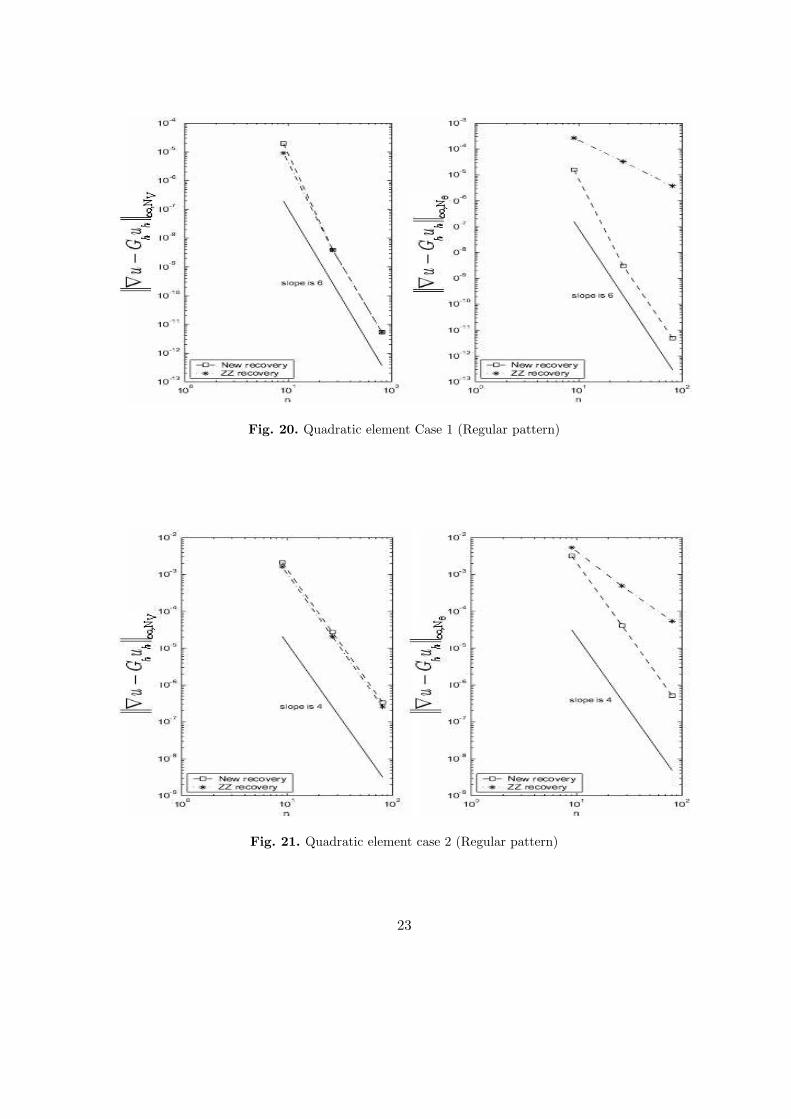
Fig. 20. Quadratic element Case 1 (Regular pattern)

Fig. 21. Quadratic element case 2 (Regular pattern)

23

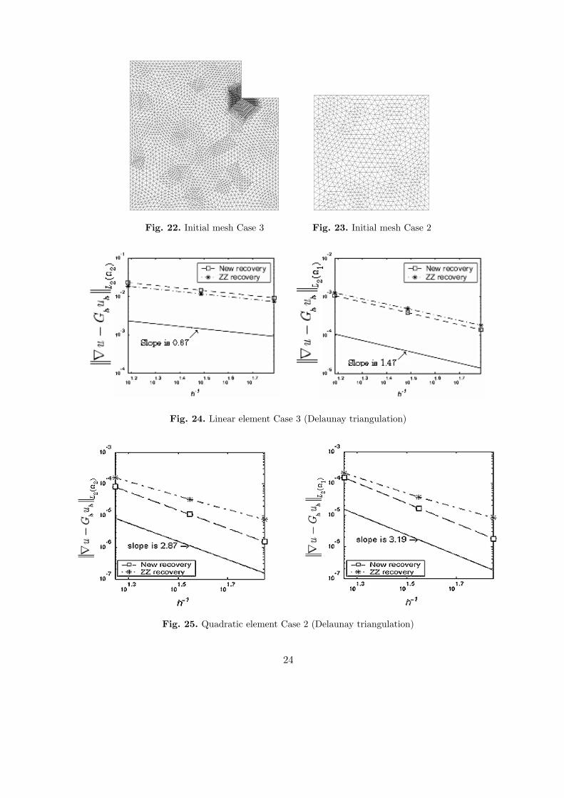
Fig. 22. Initial mesh Case 3 Fig. 23. Initial mesh Case 2

Fig. 24. Linear element Case 3 (Delaunay triangulation)

Fig. 25. Quadratic element Case 2 (Delaunay triangulation)

24

a new finite element gradient recovery method ...zzhang/paper/zhang-naga1.pdf · a new finite...

Documents