Solar Phys (2016) 291:2685–2708DOI 10.1007/s11207-015-0838-1

S U N S P OT N U M B E R R E C A L I B R AT I O N

A New Calibrated Sunspot Group Series Since 1749:Statistics of Active Day Fractions

I.G. Usoskin1,2 · G.A. Kovaltsov1,3 · M. Lockwood4 ·K. Mursula1 · M. Owens4 · S.K. Solanki5,6

Received: 27 October 2015 / Accepted: 21 December 2015 / Published online: 13 January 2016© Springer Science+Business Media Dordrecht 2016

Abstract Although sunspot-number series have existed since the mid-nineteenth century,they are still the subject of intense debate, with the largest uncertainty being related to the“calibration” of the visual acuity of individual observers in the past. A daisy-chain regressionmethod is usually applied to inter-calibrate the observers, which may lead to significant biasand error accumulation. Here we present a novel method for calibrating the visual acuity ofthe key observers to the reference data set of Royal Greenwich Observatory sunspot groupsfor the period 1900 – 1976, using the statistics of the active-day fraction. For each observerwe independently evaluate their observational thresholds [SS] defined such that the observeris assumed to miss all of the groups with an area smaller than SS and report all the groupslarger than SS. Next, using a Monte-Carlo method, we construct a correction matrix foreach observer from the reference data set. The correction matrices are significantly non-linear and cannot be approximated by a linear regression or proportionality. We emphasizethat corrections based on a linear proportionality between annually averaged data lead toserious biases and distortions of the data. The correction matrices are applied to the originalsunspot-group records reported by the observers for each day, and finally the compositecorrected series is produced for the period since 1748. The corrected series is provided as

Sunspot Number RecalibrationGuest Editors: F. Clette, E.W. Cliver, L. Lefèvre, J.M. Vaquero, and L. Svalgaard

Electronic supplementary material The online version of this article(doi:10.1007/s11207-015-0838-1) contains supplementary material, which is available to authorizedusers.

B I.G. Usoskinilya.usoskin@oulu.fi

1 ReSoLVE, Space Physics Group, University of Oulu, Oulu, Finland

2 Sodankylä Geophysical Observatory, University of Oulu, Oulu, Finland

3 Ioffe Physical-Technical Institute, St. Petersburg, Russia

4 Department of Meteorology, University of Reading, Reading, UK

5 Max-Planck Institute for Solar System Research, Göttingen, Germany

6 School of Space Research, Kyung Hee University, Yongin, Gyeonggi-Do 446-701, Korea

2686 I.G. Usoskin et al.

supplementary material in electronic form and displays secular minima around 1800 (DaltonMinimum) and 1900 (Gleissberg Minimum), as well as the Modern Grand Maximum ofactivity in the second half of the twentieth century. The uniqueness of the grand maximum isconfirmed for the last 250 years. We show that the adoption of a linear relationship betweenthe data of Wolf and Wolfer results in grossly inflated group numbers in the eighteenth andnineteenth centuries in some reconstructions.

Keywords Solar activity · Sunspots · Solar observations · Solar cycle

1. Introduction

Solar activity regularly changes in the course of the 11-year Schwabe cycle, in addition towhich it also shows slower secular variability (see, e.g., the review by Hathaway, 2015). Thisis often quantified using the sunspot-number series, which covers, with different levels ofdata quality, the period since 1610, starting with the first telescopic observations. It is gen-erally accepted (Usoskin, 2013; Hathaway, 2015) that solar activity varies between very lowactivity, called grand minima, such as the Maunder Minimum during 1645 – 1715 (Eddy,1976; Usoskin et al., 2015), and grand maxima such as the recent period of high activity inthe second half of the twentieth century, called the Modern Grand Maximum (Solanki et al.,2004).

The first attempt to produce a homogeneous sunspot-number series was made by R. Wolfin Zurich in the late nineteenth century, who produced the famous Wolf (sometimes alsocalled Zurich) sunspot-number series. This effort was continued by his successors in Zurichand finally culminated at the Royal Observatory of Belgium as the International Sunspot-Number series (Clette et al., 2014). This series uses the counting method introduced byR. Wolf, where the relative sunspot number [R] is calculated, for a given observer, as

RW = kW × (10 × G + S), (1)

where kW is the correction factor of an individual observer, and G and S are the numbersof sunspot groups and sunspots, respectively, as reported by this observer for a particularday. Unfortunately, the raw data for this series, somewhat subjectively compiled by primarypersons starting from R. Wolf, are not available in digital form, making it impossible torevisit them except for simple corrections.

A slightly different approach was proposed by Hoyt, Schatten, and Nesmes-Ribes (1994),who used only the number of sunspot groups and ignored the number of individual spots onthe disc because their number is less robustly determined. They formed the group sunspotnumber series [Rg], where a daily value for each observer was defined as

Rg = 12.08 × kg × G. (2)

Here G has the same meaning as in Equation (1), kg may be in general different from kW,and 12.08 is a scaling coefficient to match the average values of Rg and the Wolf sunspotnumber over the interval 1874 – 1976. The original data set used by Wolf was greatly up-dated, nearly doubling the number of daily sunspot records (Hoyt and Schatten, 1992; Ribesand Nesme-Ribes, 1993; Hoyt and Schatten, 1995a,b, 1996), which culminated in the re-lease of a full sunspot-group observation database (referred to as HS98 henceforth: Hoytand Schatten, 1998). HS98 provided a comprehensive database of daily values of G for allof the available observers along with the ascribed correction factors. This HS98 databaseforms a basis for further studies. Newly recovered data are being added to it continuously,along with corrections of erroneous data (e.g. Arlt, 2008; Vaquero and Vázquez, 2009; Va-

Active Day Fraction: New Sunspot Series 2687

quero et al., 2011; Arlt et al., 2013; Vaquero and Trigo, 2014; Neuhäuser et al., 2015).Thus, the database of values of G and S exists and is kept up to date. However, a majorproblem lies in the individual correction factors [k] (which may be different for differentseries) for the observers. Since the sunspot-number series is a composite series based onobservations of the Sun by a large number of individual observers with instruments of dif-ferent quality and different techniques, it is always a problem to produce a homogeneousseries, which requires an inter-calibration of the observers (Clette et al., 2014). The stan-dard way to calibrate observers to each other is based on a daisy chain of linear regressions(or even linear proportionality) between observers using periods when they overlap. Themain disadvantage of this method is that it is possible for errors to propagate and becomeaccumulated over time using multi-store regressions (a correction factor [k] is obtained byregression with a segment of other data, which has been calibrated by a regression with yetanother segment, etc.). For example, if one observer is erroneously assessed, this error willbe transferred to all other observers linked to that one. The regression is typically based ondaily values (Hoyt and Schatten, 1998), but in some cases (Svalgaard and Schatten, 2016referred to as SS15 henceforth) a proportionality between heavily smoothed (annual) valuesis used, which may lead to a serious bias, as we show in Section 4.

Several potential errors in the assessment of observers’ quality have been suggested re-cently, leading to discontinuities such as the Waldmeier discontinuity in the Wolf and In-ternational Sunspot Number (Clette et al., 2014; Lockwood, Owens, and Barnard, 2014) inthe 1940s, which are related to a change in the sunspot-counting algorithm at the Zurichobservatory; a jump between observations by Wolf and by Wolfer in the 1880s (Clette et al.,2014); and a discontinuity between Schwabe and Wolf data in 1848 (Leussu et al., 2013).Thus, a need for a revision of the sunspot series by re-calibrating individual observers hasbecome clear.

An attempt to revise the sunspot number and to produce a homogeneous data set wasmade recently by SS15, who introduced a new sunspot-group number. The method of cal-ibrating the observers in the nineteenth and twentieth century and partly in the eighteenthcentury is a modified daisy-chain regression method. They used several “backbone” ob-servers (Staudacher, Schwabe, Wolfer, and Koyama) so that all other observers are normal-ized (using a linear proportionality between annual values) to these backbones. However,since the backbones do not directly overlap with each other, a boneless bridging betweenthem is applied, again using a multi-store regression that is prone to error accumulation.This method has two shortcomings.

• First, it is “spineless”, viz. while backbones may be solid (but see below), the connectionbetween them is boneless, via stretchy multi-store regressions that accumulate errors andcannot guarantee robust normalization. We note that although the backbone method is saidby its authors to avoid daisy-chaining, this is not the case, since it includes calibration ofdata (between the backbones) derived by comparison with data from an adjacent intervalusing inter-calibration over a period of overlap between the two. Even though they usethe observer covering intermediate years to calibrate observers in earlier and later years,the errors at either step propagate between the beginning and the end of the series cal-ibrated in this way. For example, the most surprising feature of the SS15 series relatesto the amplitudes of solar cycles in the eighteenth and nineteenth centuries compared tomodern cycles: these comparisons rely on a series of daisy-chained multi-store regres-sions between the older and the modern data, regardless of the order in which they arecarried out. Daisy-chaining is a major concern because errors in each inter-calibration arecompounded over the duration of the composite data series. Avoiding daisy-chaining re-

2688 I.G. Usoskin et al.

quires a calibration method that can be applied for all data segments to the same referenceconditions, independently of the calibration of temporally adjacent data series.

• Second, the use of a linear proportionality between annually averaged data points is inap-propriate (see Section 4) and may lead to serious biases. In addition, there are, in general,a great many problems and pitfalls associated with the regressions used by daisy-chaining(Lockwood et al., 2006, 2015). The errors in the data can violate assumptions involvedin the technique, leading to grossly misleading fits, even when correlation coefficientsare high. The relationship may not be linear and a regression derived for a period of lowactivity would inherently involve gross extrapolation if applied to larger-amplitude cycles(see a discussion in Section 4). In addition, the use of the proportionality (regressions areforced through the origin) will, in general, cause amplification of the solar-cycle ampli-tudes in data from lower visual-acuity observers (Lockwood et al., 2015).

Here we propose a novel method to assess the quality of individual observers and to nor-malize them to the reference data set: the Royal Greenwich Observatory data (GreenwichPhotoheliographic Results, GPR) for the period 1900 – 1976. The method is based on acomparison between the statistics of the active-day fraction in the observer’s data and thatin the reference data set using pre-calculated calibration curves. The new method allows,for the first time, a totally independent calibration of each observer to a reference data set,without bridging them (the only exception is related to the data by Staudacher, where a two-step normalization is applied: see Section 2.3.1). The fact that this technique can be appliedto fragments of data that are not continuous with other data demonstrates that the methodavoids daisy-chaining and its associated error propagation: if one observer is calibrated er-roneously, it does not affect the other observers in any way in the new method. For eachobserver the observational threshold of the sunspot-group size is defined such that the ob-server is assumed to miss all of the groups smaller than the threshold and report all of thelarger groups. The new method allows us to assess the quality of each observer and form anew homogeneous data series of the number of sunspot groups.

2. Calibration Method

The calibration method is based on a comparison of the statistics of the active-day fraction(ADF) of the data from the observer in question with that of the reference data set. TheADF (or the related fraction of the spotless days) is a very sensitive indicator of the levelof solar activity around solar minima, which is more robust than the number of sunspots orgroups (Harvey and White, 1999; Kovaltsov, Usoskin, and Mursula, 2004; Vaquero, Trigo,and Gallego, 2012; Vaquero et al., 2015). The method includes several stages: assessing theobservational quality of individual observers, quantified as the area of sunspot groups thatthey would not have noticed; re-calibrating individual observers to the reference data set;and compiling a composite time series. These stages are described below.

2.1. Reference Data Set

We normalized all observations to the reference data set, which was selected to be the RGO(Royal Greenwich Observatory) data1 of sunspot groups, since it provides all the necessary

1We used the version of the RGO data available at the Marshall Space Flight Center (MSFC) solarscience.msfc.nasa.gov/greenwch.shtml, as compiled, maintained, and corrected by D. Hathaway. This data set isslightly different from other versions of the RGO data stored elsewhere, e.g. at the National GeophysicalData Center in Boulder CO (Willis et al., 2013a.).

Active Day Fraction: New Sunspot Series 2689

information (the observed sunspot-group areas) on a regular basis. The RGO data set, oftenalso called the Greenwich Photoheliographic Results (GPR: Baumann and Solanki, 2005;Willis et al., 2013b), was compiled using white-light photographs (photo-heliograms) of theSun from a small network of observatories, giving a data set of daily observations between17 April 1874 and the end of 1976, thereby covering nine solar cycles. The observatoriesused were the Royal Observatory, Greenwich (until 2 May 1949); the Royal GreenwichObservatory, Herstmonceux (3 May 1949 – 21 December 1976); the Royal Observatoryat the Cape of Good Hope, South Africa; the Dehra Dun Observatory, in the North-WestProvinces (Uttar Pradesh) of India; the Kodaikanal Observatory, in southern India (TamilNadu); and the Royal Alfred Observatory in Mauritius. Any remaining data gaps were filledusing photographs from many other solar observatories, including the Mount Wilson Obser-vatory, the Harvard College Observatory, Melbourne Observatory, and the US Naval Obser-vatory.

The sunspot areas were measured from the photographs with the aid of a large posi-tion micrometer (see Willis et al., 2013b and references therein). The original RGO pho-tographic plates from 1918 onwards have survived and have been digitized by the MullardSpace Science Laboratory in the UK. Automated scaling algorithms can derive sunspot areas(Çakmak, 2014), and it has been shown that the RGO data reproduce the manually scaleddaily sunspot-group numbers very well with a correlation of over 0.93 (A. Tlatov and V. Er-shov, Private communication, 2015). However, the RGO data may be subject to an unstabledata-quality problem before 1900 (Clette et al., 2014; Cliver and Ling, 2016; Willis, Wild,and Warburton, 2016). After 1977 the RGO data have been replaced by USAF–NOAA datawith a different definition of sunspot-group areas (Balmaceda et al., 2009). Accordingly,we limited the RGO reference data set to the period 1900 – 1976, which includes 28,644daily records (924 months) with full coverage. This period includes moderate-to-high so-lar activity cycles and thus leads to a conservative upper bound of the observer calibration,as discussed below. We assume that the RGO dataset corresponds to one observed by a“perfect” observer, who reports all of the sunspot groups, including the smallest one. Al-though we cannot a priori be sure that this assumption is correct, it does not affect thecalibration method. As we show below, we did not find observers in the eighteenth andnineteenth century the quality of whose data would be better than that of the RGO se-ries.

2.2. Assessing the Quality of Observers

We assumed that the “quality” of observers reporting sunspot groups is related to the size(area) of sunspot groups that they can see or report. It is quantified as the threshold area [SS](in millionths of the solar disk: msd) of the sunspot group, so that the observer would miss allof the groups with an area smaller than SS and observe all of the groups with an area greaterthan SS. We used the apparent area as seen by the observer, not corrected for foreshortening.Here we estimate this threshold area [SS].

2.2.1. Calibration Curves

First we make calibration curves based on the reference data set to assess the quality of eachobserver by comparing to these curves. The calibration curves were constructed by applyingthe following procedure:

2690 I.G. Usoskin et al.

Figure 1 The cumulativedistribution of P(A∗) (see itemiii) of Section 2.2) for thereference data set for differentvalues of the threshold observedarea [SS] as denoted in thelegend and the data coveragefraction f = 1.

i) For each day during the reference period, we counted in the reference data set the num-ber of sunspot groups with the observed whole area exceeding a given value.

ii) For each month of the reference data set, we calculated the active-day fraction (ADF)index defined as A = na/n, where na is the number of days with activity (at least onegroup is observed), and n is the number of observational days in the month. The ADFindex [A] takes values from zero (no spots observed during the month) to unity (somesunspot groups observed for every day with observations during the month).

iii) For the whole reference period (924 months), we constructed a cumulative probabilityfunction of the ADF [P (A∗) = N(A ≤ A∗)/N ], where A∗ is the given ADF valueranging between 0 and 0.9, N(A ≤ A∗) is the number of months with values of A

lower than or equal to A∗, and N is the total number of months analyzed. For example,P (0.1) = 0.029 implies that 27 months (2.9 %) out of all the months in the referencedata set have the ADF index A ≤ 0.1 This distribution is shown in Figure 1 as the solidcurve for SS = 0. Statistical uncertainties of the P -values are defined as σ0(A∗, SS) =√

N(A ≤ A∗, SS)/N(SS).iv) We repeated steps 2 and 3 above, but applying an artificial observational threshold for

the group area, viz. SS > 1, 5, 10, 15, 20, etc. (msd) using the reference data set. Thisemulates observations of an “imperfect” observer who cannot see or does not reportgroups with an area smaller than the threshold value. Distributions similar to that initem iii) were constructed for different values of SS to form a set of calibration curvesP (A,SS), as shown in Figure 1, for the range of SS from 5 to 300 msd.

v) Since real observers usually make observations on only a fraction f ≤ 1 of days, wealso emulated the effect of this and estimated the related uncertainties by a Monte-Carlo method. For each observer we defined the fraction [f ] for the entire period oftheir observation used for calibration. We repeated steps ii) – iv) above, but randomlyremoved the fraction (1-f ) of daily values from the reference data set. We did this1000 times for each combination of f and SS and thus defined an ensemble of cali-bration curves P (A,SS, f ). Next we defined the mean values of P (A,SS, f ) over theensemble that are equal within the uncertainties to P (A,SS, f = 1), and their 68 %uncertainties σ1(A,SS, f ) defined as the upper and lower 16 % quantiles. The final un-

certainty of the calibration curves P (A,SS, f ) is defined as σ(A,SS, f ) =√

σ 20 + σ 2

1 ,where σ0(A,SS, f ) is defined similarly to step iii) above, but for the random subset of

Active Day Fraction: New Sunspot Series 2691

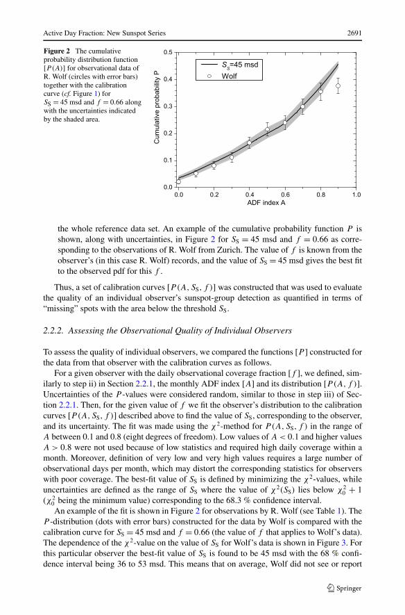
Figure 2 The cumulativeprobability distribution function[P(A)] for observational data ofR. Wolf (circles with error bars)together with the calibrationcurve (cf. Figure 1) forSS = 45 msd and f = 0.66 alongwith the uncertainties indicatedby the shaded area.

the whole reference data set. An example of the cumulative probability function P isshown, along with uncertainties, in Figure 2 for SS = 45 msd and f = 0.66 as corre-sponding to the observations of R. Wolf from Zurich. The value of f is known from theobserver’s (in this case R. Wolf) records, and the value of SS = 45 msd gives the best fitto the observed pdf for this f .

Thus, a set of calibration curves [P (A,SS, f )] was constructed that was used to evaluatethe quality of an individual observer’s sunspot-group detection as quantified in terms of“missing” spots with the area below the threshold SS.

2.2.2. Assessing the Observational Quality of Individual Observers

To assess the quality of individual observers, we compared the functions [P ] constructed forthe data from that observer with the calibration curves as follows.

For a given observer with the daily observational coverage fraction [f ], we defined, sim-ilarly to step ii) in Section 2.2.1, the monthly ADF index [A] and its distribution [P (A,f )].Uncertainties of the P -values were considered random, similar to those in step iii) of Sec-tion 2.2.1. Then, for the given value of f we fit the observer’s distribution to the calibrationcurves [P (A,SS, f )] described above to find the value of SS, corresponding to the observer,and its uncertainty. The fit was made using the χ2-method for P (A,SS, f ) in the range ofA between 0.1 and 0.8 (eight degrees of freedom). Low values of A < 0.1 and higher valuesA > 0.8 were not used because of low statistics and required high daily coverage within amonth. Moreover, definition of very low and very high values requires a large number ofobservational days per month, which may distort the corresponding statistics for observerswith poor coverage. The best-fit value of SS is defined by minimizing the χ2-values, whileuncertainties are defined as the range of SS where the value of χ2(SS) lies below χ2

0 + 1(χ2

0 being the minimum value) corresponding to the 68.3 % confidence interval.An example of the fit is shown in Figure 2 for observations by R. Wolf (see Table 1). The

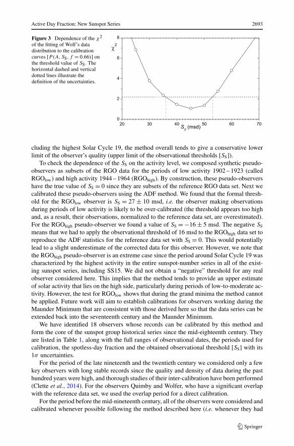
P -distribution (dots with error bars) constructed for the data by Wolf is compared with thecalibration curve for SS = 45 msd and f = 0.66 (the value of f that applies to Wolf’s data).The dependence of the χ2-value on the value of SS for Wolf’s data is shown in Figure 3. Forthis particular observer the best-fit value of SS is found to be 45 msd with the 68 % confi-dence interval being 36 to 53 msd. This means that on average, Wolf did not see or report

2692 I.G. Usoskin et al.

Table 1 Results of calibration of the key observers used here. Columns list the name of the observer; theperiod of observation [Tobs]; the period used for calibration [Tcal]; the number of observational days [N ] usedfor calibration; the data coverage in % [f ]; the fraction of spotless days [SDF] in the record; the thresholdarea [SS] in uncorrected msd; values in parentheses denote the upper and lower 1σ bound. For details seetext.

Observer Tobs Tcal N f SDF SS

RGO 1874 – 1976 1900 – 1976 28,644 ≈100 % 16 % 0

Quimby 1889 – 1921 1900 – 1921c 10,830 92 % 23 % 22(2816

)

Wolfer 1876 – 1928 1900 – 1928c 7165 68 % 21 % 6(120

)

Winklera 1882 – 1910 1889 – 1910d 4812 60 % 24 % 53(6645

)

Tacchini 1871 – 1900 1879 – 1900d 6235 78 % 19 % 10(147

)

Leppig 1867 – 1881 1867 – 1880d 2463 52 % 26 % 45(3355

)

Spoerer 1861 – 1893 1865 – 1893d 5386 53 % 15 % 3(50

)

Weber 1859 – 1883 1859 – 1883 6981 79 % 19 % 22(2816

)

Wolf 1848 – 1893 1860 – 1893d 8102 66 % 21 % 45(5336

)

Shea 1847 – 1866 1847 – 1866 5538 79 % 20 % 25(3318

)

Schmidt 1841 – 1883 1841 – 1883 6887 49 % 21 % 10(156

)

Schwabe 1825 – 1867 1832 – 1867 8570 65 % 18 % 13(188

)

Pastorff 1819 – 1833 1824 – 1833d 1451 41 % 14 % 5(100

)

Starka 1813 – 1836 1813 – 1836e 2406 30 % 41 % 60(7050

)

Derfflingera 1802 – 1824 1816 – 1824e 346 11 % 38 % 50(8040

)

Herschela 1794 – 1818 1795 – 1815 344 4 % 16 % 23(3510

)

Horrebow 1761 – 1776 1766 – 1776e 1365 34 % 27 % 75(9560

)

Schubert 1754 – 1758 1754 – 1757e 404 36 % 37 % 10(165

)

Staudacherb 1749 – 1799 1761 – 1776 1035 14 % 5.5 % –

aThe observational threshold [SS] is likely overestimated.

bCalibration is done via Horrebow (see Section 2.3.1).cDirect overlap with RGO data set.

dTo use complete cycles.eSee comments in Section 2.2.2.

sunspot groups with an (observed) area smaller than 45 msd. We also checked for a potentialsource of error in that since this method compares the ADF statistics of the real observationsto those of the reference data set, it may depend on the level of solar activity during observa-tions. If the observations were made during a period of very high activity, essentially higherthan that averaged over the reference period, this method may cause the observer’s P -curvesto appear lower because of the smaller ADF. This may lead to a potential overestimate ofthe observer’s “quality” (underestimate of their personal observational threshold [SS]) andthus to an underestimate of the solar activity based on their observational data. Conversely,for low activity, the observer’s curve may appear higher, leading to an underestimate of theirquality (overestimate of SS) and subsequently to an overestimate of solar activity. Since thecalibration curves cover a period of moderate to high levels of activity (1900 – 1976), in-

Active Day Fraction: New Sunspot Series 2693

Figure 3 Dependence of the χ2

of the fitting of Wolf’s datadistribution to the calibrationcurves [P(A,SS, f = 0.66)] onthe threshold value of SS. Thehorizontal dashed and verticaldotted lines illustrate thedefinition of the uncertainties.

cluding the highest Solar Cycle 19, the method overall tends to give a conservative lowerlimit of the observer’s quality (upper limit of the observational thresholds [SS]).

To check the dependence of the SS on the activity level, we composed synthetic pseudo-observers as subsets of the RGO data for the periods of low activity 1902 – 1923 (calledRGOlow) and high activity 1944 – 1964 (RGOhigh). By construction, these pseudo-observershave the true value of SS = 0 since they are subsets of the reference RGO data set. Next wecalibrated these pseudo-observers using the ADF method. We found that the formal thresh-old for the RGOlow observer is SS = 27 ± 10 msd, i.e. the observer making observationsduring periods of low activity is likely to be over-calibrated (the threshold appears too highand, as a result, their observations, normalized to the reference data set, are overestimated).For the RGOhigh pseudo-observer we found a value of SS = −16 ± 5 msd. The negative SS

means that we had to apply the observational threshold of 16 msd to the RGOhigh data set toreproduce the ADF statistics for the reference data set with SS = 0. This would potentiallylead to a slight underestimate of the corrected data for this observer. However, we note thatthe RGOhigh pseudo-observer is an extreme case since the period around Solar Cycle 19 wascharacterized by the highest activity in the entire sunspot-number series in all of the exist-ing sunspot series, including SS15. We did not obtain a “negative” threshold for any realobserver considered here. This implies that the method tends to provide an upper estimateof solar activity that lies on the high side, particularly during periods of low-to-moderate ac-tivity. However, the test for RGOlow shows that during the grand minima the method cannotbe applied. Future work will aim to establish calibrations for observers working during theMaunder Minimum that are consistent with those derived here so that the data series can beextended back into the seventeenth century and the Maunder Minimum.

We have identified 18 observers whose records can be calibrated by this method andform the core of the sunspot group historical series since the mid-eighteenth century. Theyare listed in Table 1, along with the full ranges of observational dates, the periods used forcalibration, the spotless-day fraction and the obtained observational threshold [SS] with its1σ uncertainties.

For the period of the late nineteenth and the twentieth century we considered only a fewkey observers with long stable records since the quality and density of data during the pasthundred years were high, and thorough studies of their inter-calibration have been performed(Clette et al., 2014). For the observers Quimby and Wolfer, who have a significant overlapwith the reference data set, we used the overlap period for a direct calibration.

For the period before the mid-nineteenth century, all of the observers were considered andcalibrated whenever possible following the method described here (i.e. whenever they had

2694 I.G. Usoskin et al.

sufficient observations to apply our technique). For each observer we used data of sunspot-group counts from the HS98 database (Hoyt and Schatten, 1998) except for Schwabe andStaudacher (see comments below). Whenever possible, we used data for complete solarcycles. Unless indicated otherwise, we considered for each observer only months with threeor more daily observations.

We also show in Table 1 the spotless-day fraction [SDF], which is the number of dayswith the reported absence of spots to the total number of observational days during thecalibration period [Tcal], for each observer. The reference RGO data set contains ≈16 % ofspotless days. SDF is in the range of 15 % to 26 % for most of the observers in the nineteenthcentury except for Stark and Derfflinger, whose observations were likely reflecting the lowactivity around the Dalton Minimum. Apparently different from all others was Staudacher,with only 57 spotless days (5.5 %) reported. He was probably more interested in drawingspots than in reporting their absence. Regardless of the reason, his statistic of spotless andactive days is distorted and cannot be used to calibrate his quality directly to the referenceperiod, as discussed in Sect. 2.3.1.

Some specific comments are given below.S.H. Schwabe observed the Sun during 1825 – 1867; but we considered only the period of

1832 – 1867 for calibration. This period covers three full cycles, since the earlier part of hisrecord is thought to be of less stable quality (Leussu et al., 2013). Sunspot-group numbersfor Schwabe’s observations were taken not from the HS98 database, but from a new revisedcollection by Arlt et al. (2013) (available at www.aip.de/Members/rarlt/sunspots/schwabe asversion 1.3 from 12 August 2015).

For J.W. Pastorff from Drossen we used data for observer 263 in the HS98 database.His SDF is low (14 % – see Table 1), indicating that he might have skipped reporting somespotless days. If this is true, it may lead to an overestimate of his observational quality andconsequently to an underestimate of the sunspot-group number based on his record. On theother hand, his corrected data are consistent with those of Schwabe and Stark (Figure 5).

C. Horrebow from Copenhagen (observer 180 in the HS98 database) observed the Sunduring 1761 – 1776. Here we used for the calibration the period of 1766 – 1776 (one solarcycle) because the data are very sparse before 1766.

T. Derfflinger from Kremsmünster observed the Sun during 1802 – 1824, but we used forthe calibration data covering 1816 – 1824 to exclude the Dalton Minimum so as to avoidthe potential problems discussed above associated with a mismatch in the range of the datacompared to that for the reference data set.

J.M. Stark from Augsburg observed the Sun during 1813 – 1836, and we used all datafor observer 255 of the HS98 database, while not considering the generic no-sunspotday records (observer #254 called “STARK, AUGSBURG, ZERO DAYS” in the HS98database).

J.C. Schubert from Danzig observed the Sun during 1754 – 1758. We used for the cali-bration the period of 1754 – 1757, which is ±2 years around the formal cycle minimum in1755.2. This includes 404 daily observations with 36 % coverage. To assess the quality ofSchubert’s observations, we used the RGO statistics, as described in Section 2.2.1, but us-ing RGO data only within ± two years around the solar-cycle minima to be consistent withSchubert’s cycle coverage.

J.C. Staudacher from Nürnberg, while providing about 1035 daily drawings for the pe-riod 1749 – 1795 (≈6 % coverage), as published by Arlt (2008), cannot be directly cali-brated in the way proposed here because he did not properly report days without sunspots.He reported no spots for only 5.5 % days, which is less than all other observers (15 – 40 %,see Table 1). Moreover, there are no zero-spot months (with the number of daily observa-tions more than two) in his record, in contrast to all other observers. This distorts the ADF

Active Day Fraction: New Sunspot Series 2695

statistics and prevents a direct calibration as described above. The case of Staudacher isconsidered separately in Section 2.3.1.

The following observers produced sufficiently long observational records but cannot becalibrated in the manner described above because of sparse or unevenly distributed observa-tions or because they did not report spotless days: Lindener, Tevel, Arago, Heinrich, Flauger-gues, and Hussey. We also did not consider observers during and around the Maunder Mini-mum because of the very low level of activity (Usoskin et al., 2015) when the method cannotbe applied. The period between the end of the Maunder Minimum and the mid-eighteenthcentury cannot be studied because of a lack of sufficient observations (Vaquero and Vázquez,2009).

In addition, we also checked the record by H. Koyama from Tokyo, who observed theSun over the period 1947 – 1984 with about 56 % daily coverage; these data formed onebackbone for the method by SS15. We used for the calibration the period of 1953 – 1976to cover full cycles, and to be more consistent with the RGO time interval; a total of 4778daily observations were processed. The calibration was performed using the reference RGOdataset for the same period of time. The threshold [SS] value was found to be 8 ± 5 msd,yielding a result fully consistent with the RGO data (see Figure 5). We stress that this recordwas not used in the compilation of the final series, but only to test the method.

The calibration method works after 1754 when Schubert started observing. If Stau-dacher’s data are included (see Section 2.3.1), the calibration starts in 1749. Before Stau-dacher there is a paucity of sufficiently long timeseries of observations by single observers,so that the method cannot work due to too poor statistics, and before 1715 the method is notapplicable because of the Maunder Minimum, where the statistics of the reference data setcannot be applied. We stopped the calibration in 1900 since the reference data set of RGOdata was used after 1900.

2.3. Corrections of Individual Observers

After we defined the observational threshold [SS] and its uncertainty for each observer (seeabove), observations (the number of sunspot groups) by this observer were calibrated to thereference data set. All corrections were made on the daily scale because of the non-linearityof correction that may otherwise distort the relation, as discussed below.

The correction for a given range of SS-values (see Table 1) was made by the Monte-Carlomethod using the reference data set of daily RGO group numbers in the following steps:

i) A test value S∗S is randomly selected, using the normally distributed random numbers,

from the distribution of SS values for the observer (see Table 1). A degraded subsetof the reference daily data set is constructed by considering only sunspot groups withthe (uncorrected) area ≥ S∗

S , i.e. what an observer with the observational limit of S∗S

would have recorded. For each daily value GS∗S

from the degraded data set we constructa distribution of the Gref-values from the reference data set (SS = 0), similar to thatshown in Figure 4b.

ii) Step i) above is repeated 1000 times, each time randomly selecting an S∗S value for a

given observer, and summing up all of the distributions of Gref for a given GS∗S

Theprobability density function (pdf) of the Gref values for each GS∗

Svalue (i.e. reported by

the observer) is constructed. Finally, the correction matrix for the particular observer isconstructed as illustrated in Figure 4a.

iii) For each daily recorded value [G] of the observer, the corresponding mean and the 68 %upper and lower quantiles of the Gref were calculated, giving the mean corrected dailygroup number and its uncertainties.

2696 I.G. Usoskin et al.

Figure 4 a: Correction matrix for the data by R. Wolf: Distribution of the daily number of groups in thereference data set Gref (ordinate) as a function of the number of groups GWolf reported by R. Wolf (abscissa).Each vertical strip is a probability density function (pdf). The grey scale is linear from 0 (white) to 1 (black)Stars represent the mean value of Gref for the given GWolf. The dotted line is the diagonal (GWolf = Gref),and the dashed red curve is the best-fit power law (GWolfer = 1.85 · G0.83

Wolf). Panel b: a cross section ofpanel a at GWolf = 5 (vertical-blue-dashed line), the star denotes the mean value of the pdf (in this caseat 7.12, making the optimum correction factor 7.12/5 = 1.424). The median at this example GWolf = 5 isGref = 7.65. Panel c: The optimum correction factor, viz. the ratio of the mean Gref to GWolf. The red-dashedline corresponds to the best-fit power law (see panel a).

The method is illustrated in Figure 4 by calibration of the observational quality of R. Wolffrom Zurich. The correction of an “imperfect” observer (R. Wolf in this example) is basedon an assessment of how many sunspot groups the “perfect” observer (the reference RGOin our case) would see for a day when the imperfect observer reported GWolf groups. Thus,for a given GWolf value (x-axis) we obtain a pdf of the reference values [Gref] to yield themean and the uncertainties of the corrected number of sunspot groups. We note that therelation is well approximated by a power law with the spectral index 0.83 (the dashed-redcurve in Figure 4), but this functional form is shown only for illustration and was not usedin the construction of correction matrices. An important feature observed is that the meanGref-value is non-zero (0.38) for spotless days reported by an imperfect observer, R. Wolf inour example. Accordingly, we cannot say whether zero spots by Wolf implies a true spotlessday or whether groups were small and went undetected. It is important that the correctionimplied by the matrix cannot be approximated by a linear (or worse still, a proportional)regression. Panel c of Figure 4 depicts the daily correction factor defined as the ratio of theGref (the number of groups the real observer would see if they were a perfect observer) toGWolf (the number of groups the observer R. Wolf actually reported). The ratio graduallydrops from ≈1.8 for one group reported by Wolf to 1.19 for 15 groups reported by Wolf. IfWolf saw 25 groups, the correction would have been only 1.02. This implies that the largerthe number of sunspot groups (the higher the activity is), the smaller the relative error ofthe imperfect observer. It is clear that a simple linear regression cannot be used to correctan imperfect observer (see Section 4). This was also emphasized by Lockwood et al. (2015)from a study of the effects of imposing different observational thresholds on the RGO data.

Active Day Fraction: New Sunspot Series 2697

Figure 5 Monthly series of sunspot-group numbers obtained by individual observers after corrections forthe observational imperfectness (uncertainties are nor shown).

From daily values for each observer, corrected for the imperfectness as described above,we calculated monthly Gref-values for individual observers, as a weighted (with weight be-ing inversely proportional to the squared error of the daily corrected value) average of theavailable daily values. We stress again that the correction should be applied to the dailyvalues, not to monthly, or even worse, annual averages, because of the non-linearity of thecorrection (see Section 4). Such series of the monthly Gref, scaled to the reference data setof RGO, are shown in Figure 5 for some individual observers. The different observers, af-ter correction, clearly agree well with one another, even though the corrections were madetotally independently for each observer.

2.3.1. Calibration of Staudacher via Horrebow

J.C. Staudacher is a key observer to evaluate solar activity in the second half of the eigh-teenth century and a backbone observer for SS15. It is crucially important to evaluate thequality of the data that he produced. However, since he apparently did not properly (see

2698 I.G. Usoskin et al.

Figure 6 The pdf matrix ofconversion of daily groupnumbers between Staudacher andHorrebow (GStaud and GHorr,respectively) using direct data foroverlapping (within ± two days)days. The grey scale is linearfrom 0 (white) to 1 (black).Orange balls are the mean values.For illustration the best-fit linearproportionality (GHorr =1.04GStaud red line) and powerlaw (GHorr = 1.91G0.69

Staud) are

shown. The two last points werenot used in the analysis.

Table 1) report spotless days, being primarily interested in drawing sunspots, the ADFmethod used here cannot be directly applied to his data, and it would yield an unrealisti-cally high quality of observations. Accordingly, we calibrated the Staudacher data in twosteps to the reference data set. This is the only exception to the method described above.

First we directly calibrated Staudacher’s data to those recorded by C. Horrebow fromCopenhagen (observer 180 of the HS98 database), whose quality is evaluated by the ADFmethod (Table 1). We used the period of direct overlap of the two observers in 1761 – 1776.Staudacher’s data were digitized recently by Arlt (2008), who processed his original draw-ings. The sunspot groups were redefined (R. Arlt, Private communication, 2015) using thesedrawings (Senthamizh Pavai et al., 2016). We note that this data set is different from theHS98 database, in particular in that it yields ≈30 % more sunspot groups. Horrebow’s datawere taken from the HS98 database as being robustly defined (R. Arlt, Private communi-cation, 2015). We found 110 days when both observers reported observations. To improvestatistics, we also compared the neighbouring ± two days. This added 101 cases when theobservations were made on successive days, and 39 days when they were separated by twodays. We note that as discussed by Willis, Wild, and Warburton (2016) in their survey of theearly RGO data, there are some sunspot groups that last for only one day, but they are infre-quent and probably near or below the SS-threshold for Staudacher and Horrebow in any case.Accordingly, the possible error introduced by using neighbouring days is greatly outweighedby the reduction in uncertainty brought about by having a greater number of samples, morethan doubling the statistics. First we checked for each daily observation by Staudacher, ifthere was a coincident record from Horrebow and took this pair if it existed in the positivecase. If such a counterpart was not found, we looked for an adjacent (±one day) observa-tion by Horrebow and took that pair if it existed. Otherwise, we considered the ± two daysinterval. This gives a total of 250 pairs of coincident data days by Staudacher and Horrebow.A cross-matrix of these daily values of Staudacher vs. Horrebow was constructed as shownin Figure 6. The two observers are clearly close to each other in the quality of observations(the matrix is nearly diagonal) except for the two right-most points, where Staudacher drewsignificantly more groups than reported by Horrebow. A matrix for converting Staudacher’sdaily values of G into Horrebow’s values was constructed in a similar way to those abovefor all other observers with respect to the reference data set.

Active Day Fraction: New Sunspot Series 2699

Next, we applied the correction matrix of the Horrebow-to-reference data set and finallyconverted Staudacher’s daily number of groups into the reference data set as follows:

GStaudR1−→ G′

HorrR2−→ Gref. (3)

For each daily value GStaud we randomly selected (step R1) the value of G′Horr from the

matrix described above (i.e. randomly from all values corresponding to GStaud), and then,for this G′

Horr we randomly selected a value of Gref from the Horrebow correction matrix(from within the row corresponding to G′

Horr). This procedure was repeated 1000 times,and finally the correction matrix of Staudacher [GStaud] daily values to the reference data set[Gref] was constructed.

2.3.2. Test of the Correction: Wolf-vs.-Wolfer

A good and important example to test our (and other) calibration methods on is the relationbetween data reported by J.R. (Rudolf) Wolf and H.A. (Alfred) Wolfer, both from the Zurichobservatory. First, a proper comparison of the two observers is crucially important as Wolfwas the reference observer for the Wolf sunspot-number series, while Wolfer is the referenceobserver for the ISN (v.2) and a backbone observer for the SS15 reconstruction. Without anadequate comparison between them, it is difficult to compare the various sunspot series nowavailable. Second, a long period of their overlap (4385 days during 1876 – 1993) exists whenboth observers independently reported sunspots. HS98, using a linear regression applied tothe daily values of the overlapping periods, proposed that the two observers are quite closeto each other in the quality of their observations. In contrast, SS15 proposed that the relationbetween them is a linear and proportional scaling so that GWolfer = 1.66GWolf, based on alinear-regression analysis of the annually averaged number of sunspot groups.

Figure 7a shows the scatter plot (in the form of a pdf as in Figure 4a) of the 4385 simul-taneous daily values of GWolfer and GWolf. Wolfer reported systematically more groups thanWolf, but the relation is significantly non-linear. In fact, as illustrated in Figure 7b, Wolfersystematically reported a few groups more than Wolf, at all levels of solar activity (see Sec-tion 4). It is evident that this non-linear relation cannot be approximated by a single linearscaling of 1.66. The black dash–dotted line represents the linear scaling 1.66 as proposed bySS15 and, although it reasonably describes low-activity periods (GWolf < 4), it progressivelyoverestimates the number of groups by Wolf for high activity. For example, for a day with10 groups reported by Wolf, this scaling would imply 16 – 17 groups reported by Wolfer.But Wolfer never reported more than 13 groups for days with GWolf = 10 (the mean forsuch days was GWolfer = 11.75). It is therefore clear that the results obtained by applyingthe linear scaling (GWolfer = 1.66GWolf) contradict the data. This is also seen in Figure 7c,which shows the scatter of the Waldmeier raw daily data and the scaled (with a factor 1.66as proposed by SS15) data of Wolf. The scaling by SS15 introduces very large errors at highlevels of solar activity, causing a moderate level to appear high. This is a primary reason ofhigh solar cycles claimed by SS15 and Clette et al. (2014) in the eighteenth and nineteenthcenturies.

Figure 7d shows the relation of the simultaneous-day group numbers by the two ob-servers, after the correction performed here (reduction to the reference RGO data set). Thedata are nearly perfectly corrected – the corrected data lie around the diagonal implyingthat both series report the same quantity. The best fit to the orange balls (the last point ex-cluded) is G∗

Wolfer = (0.98 ± 0.03)G∗Wolf, where the asterisks denote the values calibrated to

the reference data set. We recall that Wolf and Wolfer were calibrated to the reference data

2700 I.G. Usoskin et al.

Figure 7 Comparison of dailygroup numbers by Wolfer andWolf for days when both haverecords (4385 days ofsimultaneous records), presentedas a pdf (grey scale from 0(white) to 1 (black)). The orangeballs represent the mean valuesof GWolfer in each bin of GWolfvalues. The red line depicts thediagonal (GWolf = GWolf).Panel a presents raw(uncorrected) daily groupnumbers in the HS98 database.The blue-dashed line is thebest-fit power law(GWolfer = 2.03G0.77

Wolf), theblack dash-dotted line is therelation GWolfer = 1.66GWolf(used by Clette et al., 2014 andSS15). Panel b depicts thedistribution of the differencebetween GWolfer and GWolf dailygroup numbers as a function ofGWolf. Panel c presents data byWolf multiplied by 1.66 asproposed by SS15. The bluedashed curve is the best-fit powerlaw (GWolfer = 0.89 · G0.94

Wolf),Panel d presents data of bothobservers corrected to thereference conditions as proposedin this work.

set independently of each other, and thus this comparison provides a direct test of the va-lidity of the method. The ratio G∗

Wolfer/G∗Wolf should, of course, be unity if the calibration

is done correctly: that this is the derived value within the uncertainty shows that both havebeen properly estimated. Thus, since the ratio between the daily group numbers (for the dayswhen both observers made observations) of Wolf and Wolfer is consistent with unity (i.e.one-to-one relation) after each of them was independently corrected, we conclude that themethod works well. We note that this example is shown only for illustration and was notused in the actual calibration.

3. Corrected Series of Sunspot-Group Numbers

In this section we construct a composite series of sunspot-group numbers for the periodsince 1749 using the selected observers.

Active Day Fraction: New Sunspot Series 2701

3.1. Compilation of the Corrected Series

For each day [t ] we considered all those observers whose reports are available for that day.For each such observer i we took the reported Gobs,i value for that day and corrected it to thereference data set using the correction matrix for that observer (as described in Section 2.3)to define the pdf of the corresponding values [Gref]. If several observers were available forthe day, the corresponding pdfs were multiplied and re-normalized to unity again. To avoidpossible voiding of the observational days with an outlying datum, we set the minimum pdfvalues to 10−4. Then, from this composite (over all of the observers for the day) pdfs wecalculated the mean daily value of Gref and its 68 % error as the standard deviation from thegathered pdf divided by

√N , where N is the number of observers for the day.

From these composite daily series we constructed a monthly composite series as a stan-dard weighted average (see details given in, e.g. Usoskin, Mursula, and Kovaltsov, 2003) ofthe composite daily values. This series is available in the electronic supplement to the article.

Usoskin, Mursula, and Kovaltsov (2003) showed that it is not optimal to calculate theannual value of the composite series as an (arithmetic or weighted) average of the monthlyvalues. For example, if the year in question is in the rising phase of an activity cycle, thevalue of G may increase significantly between January and December, rising by up to anorder of magnitude. For example, in 1867 the monthly G was 0.15 in January and 1.6 inDecember. If by chance the coverage was better in December and the monthly error wassmaller than in January, the annual weighted mean would be dominated by the Decembervalue, which is obviously incorrect. Therefore we used a Monte-Carlo procedure to calculatethe annual G-value and its uncertainties from the daily G-values with errors:

i) For each day with existing data within the given year, we randomly took a value of dailyG from the composite pdfs of corrected daily G-values obtained above.

ii) From these randomly taken daily G-values we computed the monthly values as thesimple arithmetic mean.

iii) The annual value G′ was computed as the arithmetic mean of the monthly values.iv) Steps i) – iii) were repeated 1000 times so that a distribution of the annual G′-values was

obtained. Finally, the mean and the 68 % (divided by the√

n, where n is the number ofthe months with data in the year) were computed from the distribution. Errors propagatenaturally and without biases in this approach.

This annual series with 68 % uncertainties is shown in Figure 8. It covers the period 1749 –1899, with one missing value in 1811. To complete the series and bring it up to the presentday, we used group numbers from the RGO data set for the period 1900 – 1976. After this,we used complete series by sunspot-group numbers from the Solar Optical Observing Net-work (SOON), funded by the United States Air Force and NOAA, and filled some data gapsusing the “Solnechniye Danniye” (Solar Data, SD) Bulletins issued by the Main Astronom-ical Observatory of Russian Academy of Science (Pulkovo, St. Petersburg, Russia). TheSolar Observing Optical Network (SOON) provides images of the Sun taken in Hα line.Current sites used are RAAF Learmonth, Western Australia, Holloman AFB, New Mex-ico, USA and San Vito dei Normanni Air Station, San Vito dei Normanni, Italy. In the pastdata from telescopes at Palehua, Hawaii and Ramey Air Force Base, Puerto Rico have beenused but these are no longer operational. Calibration of the data used here was obtainedby comparison with data from Mount Wilson. The images are collected at Offutt Air ForceBase, Nebraska, USA and stored and analysed at NOAA’s National Geophysical Data Cen-ter (NGDC) in Boulder. Unlike the RGO data, the SOON data are recorded as drawings andnot as photographic plates. We used the RGO-SOON group number intercalibration derived

2702 I.G. Usoskin et al.

Figure 8 Annual number ofsunspot groups for the period1749 – 1900 (solid curve)normalized to the reference dataset, along with 68 % confidenceinterval (grey shading). Thereference data set of RGO groupnumbers for 1900 – 1976,extended by the SOON data1977 – 2013, as normalized to theRGO set by Lockwood, Owens,and Barnard (2014), isrepresented by the dotted curve.

by Lockwood, Owens, and Barnard (2014), which employs the international sunspot num-ber as a spline and minimizes the difference between the means of the fit residuals for beforeand after the RGO/SOON join.

The activity remains at a moderate level in the nineteenth century and is higher in theeighteenth century. However, activity (sunspot-group numbers) in both the eighteenth andnineteenth centuries remained significantly lower than the Modern Grand Maximum in thesecond half of the twentieth century.

We also note that there is another source of non-linearity not accounted for here (neitherwas it considered in previous series, such as HS98, ISN, or SS15). It is related to the cal-culation of monthly and annual values from a small number of sparse daily observations.Under these conditions, the simple arithmetic average tends to overestimate the number ofsunspots (groups) for active periods if the number of daily observations per month is smallerthan three (Usoskin, Mursula, and Kovaltsov, 2003). The overestimate can be as much as20 – 25 %. This may affect the values for the eighteenth century, where data coverage waslow. Since this effect leads to a possible overestimate of the monthly (and thus annual) val-ues, it keeps the averaged series provided here as a conservative upper limit. However, thiseffect does not influence the calibration and correction procedure that works with the orig-inal daily data. Neither is the corrected daily series affected. This effect will be taken intoaccount in forthcoming studies.

3.2. Comparison to Previous Reconstructions

Here we compare the new series with two earlier series of the number of sunspot groups:the GSN series by HS98 based on consecutive mutual calibration of observers; and therecent series by SS15 based on a composite of backbone, high-low activity, and brightest starmethods. In Figure 9 we show these series along with the recent reconstruction of sunspotactivity around the Maunder Minimum using active-day statistics (Vaquero et al., 2015).

The new series is close to the GSN series by HS98, being consistent with it within un-certainties after ≈1830 and yielding Solar Cycles 10 and 11 to be slightly higher than in theHS98 series. The newly reconstructed cycles are significantly higher than the HS98 valuesbefore 1830. On the other hand, the new series is consistently lower than the values proposedby SS15, except for the years of the sunspot-cycle minima. This difference is mostly due tothe linear regression used by SS15 to correct the Wolf-vs.-Wolfer records, which leads to abias, as discussed in Section 4. Before 1830 the new series lies between the HS98 and SS15series, on one hand being consistent with the conclusion by SS15 that the HS98 GSN is most

Active Day Fraction: New Sunspot Series 2703

Figure 9 Comparison ofdifferent series of annualnumbers of sunspot groups G:solid-black curve – the presentreconstruction (identical to thatshown in Figure 8); red-dottedcurve – group sunspot number(HS98) divided by 12.08;blue-dashed curve – number ofgroups reconstructed by SS15;green-dotted curve – sunspotnumber divided by 12.08 aroundthe Maunder Minimum asreconstructed by the strict modelof Vaquero et al. (2015). Thelower panel is the differencebetween the two other G-seriesshown in the upper panel and thepresent result, for the period1749 – 1899. We also plot in thelower panel (shaded area) the68 % uncertainty estimate of thepresent data set.

likely too low before the Dalton Minimum, but on the other hand implying that the revisionby SS15 is too high. We recall that because of the moderate-to-high activity underlying thereference data set, our reconstruction tends to overestimate reconstructed activity at earliertimes with lower activity. We note that the RGO data and the SS15 series also diverge around1945, and tests by Lockwood, Owens, and Barnard (2016) against independent data indicatethat this is another error in the backbone reconstruction. The two errors (around 1945 andthe Wolf-vs.-Wolfer relationship) both act in the same direction, to make early group sunspotnumbers too large in relation to those in the Modern Grand Maximum.

The new reconstruction suggests that the sunspot activity (quantified as the numberof groups) was somewhat higher in the mid-eighteenth century than it was in the mid-nineteenth century, but significantly lower than the Modern Grand Maximum (Usoskin et al.,2003; Solanki et al., 2004) in the second half of the twentieth century. The Dalton (ca. 1800)and Gleissberg (ca. 1900) Minima of solar activity are clearly seen as the reduced magni-tude of solar cycles, but they are not considered as grand minima of activity in contrast tothe Maunder Minimum (Usoskin, 2013).

4. A Note on Non-linearity and the Lack of Proportionality

The main reason for the difference between the sunspot-activity levels resulting from thiswork and previous recent reconstructions (e.g. Clette et al., 2014; Svalgaard and Schatten,2016) is that the latter were based on linear regressions between annually averaged data ofindividual observers, which can seriously distort the results. Furthermore, SS15 assumedproportionality between the data (by forcing linear regressions through the origin and usingonly scaling correction factors without offsets), which is also incorrect and leads to possi-ble errors that accumulate because the backbone calibrations are daisy-chained (Lockwoodet al., 2015). For example, the linear regression suggests a ratio of 1/0.6 = 1.66 between thenumbers of sunspot groups reported by Wolf and Wolfer. This assumes that Wolf was miss-

2704 I.G. Usoskin et al.

Figure 10 Assessment ofsmall-size groups that might havebeen missed by R. Wolf using thestatistics of the reference data set(daily RGO sunspot groups withtheir size for the period1900 – 1976) as shown inFigure 4a. Panel a: the fraction ofthe potentially missed sunspotgroups as a function of thenumber of sunspot groups visiblefor Wolf. Panel b: the absolutenumber of potentially missedsunspot groups as a function ofthe number of sunspot groupsvisible for Wolf. The solid dotsand the grey shading depict themean and the 68 % confidenceintervals, respectively. The dottedline indicates the constant 40 %fraction of missed spot groups asassumed by the linear regression.

ing 40 % of all groups that would have been observed by Wolfer, regardless of the activitylevel, viz. a no-spot record by Wolf would correspond to no spots observed by Wolfer, but15 groups reported by Wolf would correspond to 25 groups by Wolfer. As we show here,a linear regression (proportionality) based on the annually averaged data may lead to signif-icant biases leading to a heavy overestimation of the number of sunspot groups recorded byWolf during the periods of high activity.

The relation between records of different observers is non-linear (see, e.g., Figure 4a forWolf). First, it does not necessarily go through the origin (0 – 0 point). Thus GWolf = 0 yieldsa non-zero Gref with a mean of 0.49 and the 68 % range from 0 to 2 groups. This indicatesthat when Wolf reported no spots, there might have been 0 – 2 groups on the Sun. Thisfeature is totally missed when assuming a linear proportionality. The relation between Wolfand Wolfer is quite steep (the slope of a regression forced through the origin is about 1.7)for low activity days (1 – 2 groups), but then the slope of the relation drops (see Figure 4c)to almost unity for days with more than 20 groups. It is obvious that a single correctionfactor is not applicable for such a relation as it assumes that an imperfect observer (Wolfin this case) misses the same fraction of spots regardless of the activity level. However, thenon-linearity of the relation arises because an observer with a poorer instrument or eyesight,or observing in poorer conditions, does not see and report the smallest spots as defined bytheir observational threshold [SS].

It is important that the fraction of small spots is not constant, as proposed by the linearcorrection, but depends strongly on the level of solar activity. It is usually large for a smallnumber of groups and small for multiple groups, as illustrated in Figure 10 for the case ofWolf. While the fraction of small groups (panel a), potentially missed by Wolf, is as high as45 % for the days when he would report only one sunspot group, it drops very quickly, sothat it is only 21 % for days with 10 groups reported and 10 % for very active days with thenumber of reported groups being 16. The assumption of a constant fraction of missed groups(the dotted line) does not describe the distribution, and it heavily overestimates the missed

Active Day Fraction: New Sunspot Series 2705

group for moderate and high activity. Panel b shows that for moderate and high activity(daily G > 4), Wolf would have been missing the same amount of 2 – 3 groups on average,regardless of the exact number of groups that he saw (cf. Figure 7b). The assumption ofthe constant fraction of missed groups (the dotted line with the slope 0.6667 = 0.4/0.6) isapparently invalid and is applicable only for low-activity days (G < 4). This suggests thatnot a multiplicative (via a scaling factor) but an additive (with an offset) correction would bemore appropriate for moderate-to-high activity days. However, the most appropriate way tocorrect a given observer (Wolf in this example) is to apply the correction matrix (Figure 4)to daily group numbers observed by them as described here.

Another problem with linear regressions is that because of the non-linearity, the averag-ing procedure is not transmissive for corrections, i.e. the correction of the averaged valuesis different from the average of corrected values. Corrections must be applied to daily val-ues using a matrix as shown in Figure 4, and only after that can the corrected values beaveraged to monthly or yearly resolution, as described in Section 2.3. Corrections appliedto (annually) averaged values miss the non-linearity and, since the annual values are domi-nated by low and moderate numbers of groups, lead to an overestimate of the relation and,as a consequence, to too high solar cycles. Moreover, the use of simple arithmetic meansfrom sparse daily values may lead to an additional overestimate of the monthly (or annual)values, thus distorting the relation (Usoskin, Mursula, and Kovaltsov, 2003, see discussionin Section 3.1). A weighted average should be used instead.

Accordingly, the use of annual (or even monthly) averaged values for a linear scalingcorrection is not appropriate and is grossly misleading.

A different average size of sunspot groups as a function of activity level producing sucha non-linearity is known in solar physics (e.g. Solanki and Unruh, 2004). E.g., the ratioof faculae to spots changes with activity level (i.e. the ratio of number of small to largemagnetic flux tubes). Of course, neither faculae-to-spot area ratio nor sunspot areas directlyenter into the number of sunspot groups or the size of groups, but they are examples of other(somewhat related) quantities showing a non-linear behaviour.

5. Conclusions

A new series of sunspot-group numbers, based on a novel method of independently cal-ibrating the quality of data by different sunspot observers, was presented for the period1749 – 1900. These data were calibrated using the data from the Royal Greenwich Observa-tory for the period 1900 – 1976 as a reference, which is readily extended to the present dayusing the SOON data, forming a homogeneous series for the entire period since 1749 – 1976(see Figure 8). The new series is a composite of 18 individual observers (Table 1), each be-ing independently calibrated to the reference data set using the newly developed active-dayfraction method. It is important that the new method provides independent direct calibration,using the active-day-fraction statistics, of the observers to the reference data set in the senseof the observational threshold, thus avoiding consecutive error accumulation, in contrast toearlier methods. The method includes several main steps:

i) constructing calibration curves for the reference data set;ii) assessing the quality of individual observers in terms of the observational threshold of

the sunspot-group area [SS];iii) normalizing raw data by the individual observers to the reference data set;iv) compiling the composite series.

2706 I.G. Usoskin et al.

The method does not use any linear regressions or other prescribed functional relations,but is, instead, based on a direct correction matrix and the Monte-Carlo method. The basicassumptions of the method are as follows:

• The reference data set is of the “perfect” quality, and the ADF statistic for this set isrepresentative for the entire period under investigation. The selection of the reference dataset ensures that violations of this assumption may only lead to a possible overestimate ofthe activity.

• The quality of an observer is quantified as the observational threshold [SS], so that theobserver misses all groups with an area smaller than SS and reports all groups with anarea greater than SS, and the quality remains constant throughout their entire period ofobservations, but this can be revisited in the future by a piece-wise calibration.

• The correction of an “imperfect” observer is based on an estimate of the number of groupsthat they would see if they were a “perfect” observer (i.e. with the data quality correspond-ing to the reference data set).

The series presented here is a basic skeleton, or core, of the reconstruction of the numberof sunspot groups, to which other observers with shorter sunspot records can and will beadded later by means of direct normalization to this core series. The raw series includes dailynumbers of sunspot groups, the mean values and their 68 % confidence intervals, reduced tothe reference data set, for each individual observer listed in Table 1. The composite seriesexists, in addition to raw daily resolution, as monthly and annual averages provided in theelectronic supplementary material.

The new series is consistent with the group sunspot number (Hoyt and Schatten, 1998) af-ter about 1830, but is systematically higher than that in the eighteenth century, implying thatthe sunspot activity was higher than proposed by HS98 before the Dalton Minimum. Con-versely, the new series is significantly and systematically lower than the backbone sunspot-group number SS15 in the nineteenth and eighteenth century, implying that the backbonereconstruction grossly overestimates solar activity during that period. We demonstrated thatthe overestimate of the backbone method was caused by the incorrect use of linear propor-tionality to normalize the observers to each other, which led to propagation and accumula-tion of errors. Furthermore, the use of annual means of sparse data led to additional errors,enhancing those for observers active at earlier times.

The new series depicts lows of solar activity around 1800, known as the Dalton Mini-mum, and around 1900, known as the Gleissberg Minimum, although they are not consid-ered as grand minima of activity. We note that the new series provides an upper limit for thegroup numbers during most of the times, in particular around the Dalton Minimum, whenboth the activity level and the observation density were low. The Modern Grand Maximumof activity in the twentieth century is confirmed as a unique event over the last 250 years.This confirms and enhances the established pattern of the secular variability of solar activity(e.g. Hathaway, 2015; Usoskin, 2013).

Acknowledgements We are thankful to Rainer Arlt for the revised data of Staudacher. Contributions fromI. Usoskin, K. Musrsula, and G. Kovaltsov were done in the framework of the ReSoLVE Centre of Excellence(Academy of Finland, project no. 272157). Work at the University of Reading is supported by the UK Scienceand Technology Facilities Council under consolidated grant number ST/M000885/1. G. Kovaltsov acknowl-edges partial support from Programme No. 7 of the Presidium RAS. This work was partly supported by theBK21 plus program through the National Research Foundation (NRF) funded by the Ministry of Educationof Korea.

Disclosure of Potential Conflicts of Interest The authors declare that they have no conflicts of interests.

Active Day Fraction: New Sunspot Series 2707

References

Arlt, R.: 2008, Digitization of sunspot drawings by Staudacher in 1749 – 1796. Solar Phys. 247, 399. DOI.ADS.

Arlt, R., Leussu, R., Giese, N., Mursula, K., Usoskin, I.G.: 2013, Sunspot positions and sizes for 1825 – 1867from the observations by Samuel Heinrich Schwabe. Mon. Not. Roy. Astron. Soc. 433, 3165. DOI.

Balmaceda, L.A., Solanki, S.K., Krivova, N.A., Foster, S.: 2009, A homogeneous database of sunspot areascovering more than 130 years. J. Geophys. Res. 114, A07104. DOI. ADS.

Baumann, I., Solanki, S.K.: 2005, On the size distribution of sunspot groups in the Greenwich sunspot record1874 – 1976. Astron. Astrophys. 443, 1061. DOI. ADS.

Çakmak, H.: 2014, A digital method to calculate the true areas of sunspot groups. Exp. Astron. 37, 539. DOI.ADS.

Clette, F., Svalgaard, L., Vaquero, J.M., Cliver, E.W.: 2014, Revisiting the sunspot number: A 400-year per-spective on the solar cycle. Space Sci. Rev. 186, 35. DOI.

Cliver, E.W., Ling, A.G.: 2016, The discontinuity in ∼1885 in the group sunspot number. Solar Phys. DOI.Eddy, J.A.: 1976, The Maunder minimum. Science 192, 1189. DOI. ADS.Harvey, K.L., White, O.R.: 1999, What is solar cycle minimum? J. Geophys. Res. 104, 19759. DOI. ADS.Hathaway, D.H.: 2015, The solar cycle. Living Rev. Solar Phys. 12, 4. DOI. http://www.livingreviews.org/lrsp-

2015-4.Hoyt, D.V., Schatten, K.H., Nesmes-Ribes, E.: 1994, The one hundredth year of Rudolf Wolf’s death: Do we

have the correct reconstruction of solar activity? Geophys. Res. Lett. 21, 2067. DOI. ADS.Hoyt, D.V., Schatten, K.H.: 1992, New information on solar activity, 1779 – 1818, from Sir William Her-

schel’s unpublished notebooks. Astrophys. J. 384, 361. DOI. ADS.Hoyt, D.V., Schatten, K.H.: 1995a, A new interpretation of Christian Horrebow’s sunspot observations from

1761 to 1777. Solar Phys. 160, 387. DOI. ADS.Hoyt, D.V., Schatten, K.H.: 1995b, A revised listing of the number of sunspot groups made by Pastorff, 1819

to 1833. Solar Phys. 160, 393. DOI. ADS.Hoyt, D.V., Schatten, K.H.: 1996, How well was the sun observed during the Maunder minimum? Solar Phys.

165, 181. DOI. ADS.Hoyt, D.V., Schatten, K.H.: 1998, Group sunspot numbers: A new solar activity reconstruction. Solar Phys.

179, 189. DOI. ADS.Kovaltsov, G.A., Usoskin, I.G., Mursula, K.: 2004, An upper limit on sunspot activity during the Maunder

minimum. Solar Phys. 224, 95. DOI. ADS.Leussu, R., Usoskin, I.G., Arlt, R., Mursula, K.: 2013, Inconsistency of the Wolf sunspot number series

around 1848. Astron. Astrophys. 559, A28. DOI.Lockwood, M., Owens, M.J., Barnard, L.: 2016, Tests of sunspot number sequences: 4. The “Waldmeier

discontinuity” in various sunspot number and sunspot group number reconstructions. Solar Phys., thisissue.

Lockwood, M., Owens, M.J., Barnard, L.: 2014, Centennial variations in sunspot number, open solar flux,and streamer belt width: 1. Correction of the sunspot number record since 1874. J. Geophys. Res. 119,5172. DOI. ADS.

Lockwood, M., Rouillard, A.P., Finch, I., Stamper, R.: 2006, Comment on “The IDV index: Its derivation anduse in inferring long-term variations of the interplanetary magnetic field strength” by Leif Svalgaardand Edward W. Cliver. J. Geophys. Res. 111, A09109. DOI. ADS.

Lockwood, M., Owens, M.J., Barnard, L., Usoskin, I.G.: 2015, in press, Tests of sunspot number sequences:3. Effects of regression procedures on the calibration of historic sunspot data. Solar Phys.

Neuhäuser, R., Arlt, R., Pfitzner, E., Richter, S.: 2015, Newly found sunspot observations by Peter Beckerfrom Rostock for 1708, 1709, and 1710. Astron. Nachr. 336, 623. DOI. ADS.

Ribes, J.C., Nesme-Ribes, E.: 1993, The solar sunspot cycle in the maunder minimum ad1645 to ad1715.Astron. Astrophys. 276, 549.

Senthamizh Pavai, V., Arlt, R., Diercke, A., Denker, C., Vaquero, J.M.: 2016, Sunspot group tilt angle mea-surements from historical observations. Adv. Space Res., submitted.

Solanki, S.K., Unruh, Y.C.: 2004, Spot sizes on Sun-like stars. Mon. Not. Roy. Astron. Soc. 348, 307. DOI.ADS.

Solanki, S.K., Usoskin, I.G., Kromer, B., Schüssler, M., Beer, J.: 2004, Unusual activity of the sun duringrecent decades compared to the previous 11,000 years. Nature 431, 1084. DOI. ADS.

Svalgaard, L., Schatten, K.H.: 2016, Reconstruction of the sunspot group number: the backbone method.Solar Phys. DOI.

Usoskin, I.G., Mursula, K., Kovaltsov, G.A.: 2003, Reconstruction of monthly and yearly group sunspotnumbers from sparse daily observations. Solar Phys. 218, 295. DOI.

Usoskin, I.G.: 2013, A history of solar activity over millennia. Living Rev. Solar Phys. 10, 1. DOI. ADS.

2708 I.G. Usoskin et al.

Usoskin, I.G., Arlt, R., Asvestari, E., Hawkins, E., Käpylä, M., Kovaltsov, G.A., Krivova, N., Lockwood, M.,Mursula, K., O’Reilly, J., Owens, M., Scott, C.J., Sokoloff, D.D., Solanki, S.K., Soon, W., Vaquero,J.M.: 2015, The Maunder minimum (1645 – 1715) was indeed a grand minimum: A reassessment ofmultiple datasets. Astron. Astrophys. 581, A95. DOI. ADS.

Usoskin, I.G., Solanki, S.K., Schüssler, M., Mursula, K., Alanko, K.: 2003, Millennium-scale sunspot numberreconstruction: Evidence for an unusually active sun since the 1940s. Phys. Rev. Lett. 91, 211101. DOI.ADS.

Vaquero, J.M., Trigo, R.M.: 2014, Revised group sunspot number values for 1640, 1652, and 1741. SolarPhys. 289, 803. DOI. ADS.

Vaquero, J.M., Vázquez, M.: 2009, The Sun Recorded Through History: Scientific Data Extracted from His-torical Documents, Astrophys. Space Sci. Lib. 361, Springer, Berlin. ADS.

Vaquero, J.M., Trigo, R.M., Gallego, M.C.: 2012, A simple method to check the reliability of annual sunspotnumber in the historical period 1610 – 1847. Solar Phys. 277, 389. DOI. ADS.

Vaquero, J.M., Gallego, M.C., Usoskin, I.G., Kovaltsov, G.A.: 2011, Revisited sunspot data: A new scenariofor the onset of the Maunder minimum. Astrophys. J. Lett. 731, L24. DOI. ADS.

Vaquero, J.M., Kovaltsov, G.A., Usoskin, I.G., Carrasco, V.M.S., Gallego, M.C.: 2015, Level and length ofcyclic solar activity during the maunder minimum as deduced from the active day statistics. Astron.Astrophys. 577, A71. DOI.

Willis, D.M., Wild, M.N., Warburton, J.S.: 2016, Re-examination of the daily number of sunspot groups forthe Royal Observatory, Greenwich (1874 – 1885). Solar Phys., this issue.

Willis, D.M., Henwood, R., Wild, M.N., Coffey, H.E., Denig, W.F., Erwin, E.H., Hoyt, D.V.: 2013a,The Greenwich photo-heliographic results (1874 – 1976): Procedures for checking and correcting thesunspot digital datasets. Solar Phys. 288, 141. DOI. ADS.

Willis, D.M., Coffey, H.E., Henwood, R., Erwin, E.H., Hoyt, D.V., Wild, M.N., Denig, W.F.: 2013b,The Greenwich photo-heliographic results (1874 – 1976): Summary of the observations, applications,datasets, definitions and errors. Solar Phys. 288, 117. DOI. ADS.