a new binary logarithmic arbitration method for ethernet

A New Binary Logarithmic Arbitration Method for Ethernet

Mart L. Molle

Technical Report CSRI-298April 1994

(Revised July 1994)

Computer Systems Research InstituteUniversity of Toronto

Toronto, CanadaM5S 1A1

The Computer Systems Research Institute (CSRI) is an interdisciplinary group formed to conduct research anddevelopment relevant to computer systems and their application. It is an Institute within the Faculty of Applied Sci-ence and Engineering, and the Faculty of Arts and Science, at the University of Toronto, and is supported in part bythe Natural Sciences and Engineering Research Council of Canada.

Copyright 1994, Mart L. Molle

1

A New Binary Logarithmic Arbitration Method for Ethernet

Mart L. MolleComputer Systems Research Institute

Department of Computer ScienceUniversity of Toronto

Toronto, Canada M5S 1A4

Abstract — Recently, Ethernet celebrated its twentieth anniversary. Over those years, the processingspeed of the attached hosts has increased by several orders of magnitude, to the point where the relativebandwidth of a 10 Mbps Ethernet has fallen from more than adequate to support large enterprise networks(whose utilizations were typically only a few percent, anyway), to marginally fast enough to support asingle high performance desktop workstation. At the same time, the Ethernet standard has also evolvedto incorporate new technology at the physical layer, including new media, new signalling methods, andsupport for higher data rates. However, the MAC layer protocols have remained essentially unchangedfrom the early days of undemanding applications running on large numbers of slow hosts. In this paper,we argue that it is time to review the MAC layer and incorporate advances made in the protocol perfor-mance field over the last twenty years. First, we describe several little-known facts about the dynamicbehaviour of the current Truncated Binary Exponential Backoff (BEB) algorithm, and explain how thesefeatures can cause significant performance problems for a variety of interesting network configurations.We then show that the backoff algorithm can be modified to eliminate all of these performanceanomalies, without sacrificing performance or interoperability with existing Ethernet compatible devices.Indeed, the actual performance characteristics of the resulting algorithm, which we call the Binary Loga-rithmic Arbitration Method (BLAM), closely follow the stated design goals for BEB.

I. Performance Implications of the Current MAC Layer Protocol

I.a. How Ethernet is Used

The original design goals for Ethernet were ‘‘to design a communication system which can growsmoothly to accommodate several buildings full of personal computers [emphasis added] and the facili-ties needed for their support’’ [21]. In other words, the environment for which it was designed consistedof a large, loosely-coupled collection of slow hosts (such as the Xerox Alto minicomputer [30]), that usedthe network for occasional access to such services as archival file servers, shared printers, etc. Althoughno SPECmark rating is available for the Alto, its relative slowness (compared to Ethernet) should beobvious from the fact that simple address filtering in the presence of back-to-back minimum-length pack-ets was reported to use up 20% of the CPU [30].

Of course, present day hosts have much more processing power than an Alto, and new styles ofnetwork interaction have emerged, including remote file systems, diskless workstations, X-terminals,multimedia, and more. High end desktop workstations can easily saturate a 10Mbps Ethernet, and (as ofFall 1992) a few could even saturate a 100Mbps FDDI ring. Thus, at the present time few people wouldrecommend trying to support more than a few dozen hosts on a single 10Mbps Ethernet. (Of course,100Mbps Ethernet would provide sufficient bandwidth to support several hundred hosts with similartraffic demands.) Indeed, 10Mbps may even be seen as a performance bottleneck for a single high perfor-mance workstation being used in a data-intensive application like multimedia, computer aided design, ordata visualization.

2

Below, when we discuss the implications of various performance issues, we will illustrate theproblems in terms of their effects on following three classes of network usage. The first is a workgroupof personal computers, in which a collection of reasonably autonomous users need occasional access toshared resources. This is precisely the environment that was envisioned by the original designers of Eth-ernet. The second class is the power users, who run data-intensive applications on high performanceworkstations. The third class involves backbone interconnection to tie together various server machines,or to connect high performance hosts directly to the backbone network (perhaps some higher-speedenterprise-wide network, or an ATM switch).

I.b. Stability, Capacity and the Channel Capture Effect

Ethernet uses a random-access MAC layer protocol, belonging to the Aloha, CSMA, andCSMA/CD protocol families. A necessary requirement for using one of these protocols is solving the sta-bility question: collisions waste channel bandwidth, and collisions generate more collisions through apositive feedback effect where the retransmitted packets compete with future arrivals to make the load onthe channel tend to grow with time. Fortunately, it was rigorously proven more than 20 years ago thatsuch protocols could be stabilized by employing a suitable dynamic control procedure for reschedulingpackets after each collision [10]. Since then, many suitable control algorithms have been found[9, 14, 20]. Unfortunately, the stability of Ethernet’s binary exponential backoff is somewhat open todebate. On the one hand, a well-known textbook makes the unsubstantiated claim that ‘‘The only generalstatement that is inarguable is that an overloaded 802.3 LAN will collapse totally . . .’’ [29, p. 164],whereas published measurement studies [6] of actual Ethernet performance under overload provide astrong counterexample to that claim (at least when the number of hosts contributing to the overload situa-tion is relatively small, since their testbed only contained 24 hosts).

There are also conflicting results in the theoretical literature. For example, Aldous [3] provedthat a non-truncated version of the algorithm is unstable for any non-zero throughput value in the limit ofan unbounded number of hosts. This is because the average packet delay in such a system would beinfinite, since a certain proportion of the packets will never be delivered, no matter how many retransmis-sion attempts were allowed. On the other hand, Goodman et al. [12] showed that it is stable for a systemcontaining limited number of buffered hosts. Unfortunately, as first noted by Shenker [24], the dynamicsof that channel sharing essentially represent the worst-possible scheduling discipline. That is, the timerequired to acquire the channel to send the next packet in the transmit queue resembles a ‘‘reverse lot-tery’’: most packets get sent as soon as they reach the head of the transmit queue, but a few suffer spec-tacularly large delays. We will come back to discuss the delay implications of this variability in the nextsection. For now, we will limit our discussion to an explanation of its causes.

Recall that under BEB, the updates to the collision counter at each host are done independently,and only in response to actual transmission attempts by the given host. Thus, in particular, only the‘‘winner’’ gets to reset its collision counter after a successful packet transmission. This asymmetry in thetreatment of the collision counters can permit a single busy host to ‘‘capture’’ the network for anextended period of time, in the following way. If we examine the system during a contention interval,when several active hosts are competing for control of the channel, we would expect each of them to pos-sess a non-zero collision counter. Eventually, one of those hosts will acquire the channel and deliver itspacket. At the next end-of-carrier event, the remaining hosts will still have non-zero collision countervalues, but the ‘‘winning’’ host will reset its collision counter to zero before returning to the competition.If the ‘‘winning’’ host has more packets in its transmit queue (and its network interface is fast enough), itis free to transmit its next packet immediately. Conversely, the rest of the hosts may be delayed untiltheir latest backoff interval expires. Furthermore, should any of them collide with the ‘‘winning’’ host,observe that the ‘‘winner’’ randomizes its first retry over the smallest possible backoff interval, whereas

3

the other hosts randomize their next retry over a (much) larger interval. Thus, the same host is likely to‘‘win’’ a second time, in which case the same situation will be repeated at the next end-of-carrier eventexcept the other hosts’ collision counters have gotten larger. Thus, it is even more likely that thewinner’s ‘‘run’’ of good luck will continue until its transmit queue is emptied, or some other especially-unlucky host’s collision counter ‘‘wraps around’’ after 16 failed attempts — causing it to compete moreaggressively for control of the channel after reporting an excessive collision error.

Although the Ethernet capture effect can cause significant short-term unfairness (in terms of thechannel access delays experienced by different hosts), one must not forget the fact that it can also helpperformance under some circumstances. In particular, capture increases the capacity of the network byallowing a host to spread the ‘‘cost’’ of acquiring the channel during an Ethernet MAC layer contentionperiod over multiple packet transmissions. Let us define the normalized capacity of a network to be theratio of the maximum sustainable throughput (in bits/sec) to the raw channel data rate (in bits/sec) for thegiven combination of packet sizes and numbers/locations of hosts, without regard for the resulting packetdelays. Generalizing the simple renewal-type argument described by Metcalfe and Boggs in [21] toaccount for the capture effect, we will describe the operation of the network as a sequence of ‘‘cycles’’,each consisting of an Aloha-type contention period followed by a (‘‘run’’ of) packet transmission(s) bythe ‘‘winning’’ host. In this case, the normalized capacity may be expressed as the ratio of the averagetime required to transmit all the packets in the ‘‘run’’ divided by the average duration of the entire‘‘cycle’’ (including its associated contention period). By assuming that the number of active hosts islarge and taking a macroscopic view of the network (where the details of the state of the backoff algo-rithm at each host are ignored), Metcalfe and Boggs used the slotted Aloha formula to estimate the aver-age length of a contention period. Under this model, we assume that roughly one out of every e conten-tion slots will initiate the successful transmission of a packet by one of the active hosts, where e∼∼2.7071is the base of the natural logarithm. Thus, if the the average packet length is B bits and the average‘‘run’’ length is K packets per cycle, then we obtain the following estimate for the normalized capacity:

K .B + (e − 1).512K .B� �� .

Using this formula, we can obtain capacity estimates for various combinations of packet sizes andrun lengths, similar to those presented in [21, Table I]. For example, if the average packet length is large(e.g., 1500 bytes), then even without the capture effect the formula shows that the normalized capacity isin excess of 0.93. On the other hand, if the average packet length is small (e.g., the worst-case value of64 bytes), then in the absence of capture (i.e., K .B = 512), the above capacity estimate drops to1/e ∼∼ 0.368, which is the capacity of slotted Aloha. However, much higher capacities are possiblebecause of the capture effect, if we allow the ‘‘run’’ lengths to grow sufficiently large. For example, aswe increase the average run lengths to K = 2, 4, 8, 16, . . . the estimated capacity increases monotonicallyto 0.538, 0.700, 0.823, 0.903, . . . respectively. But notice that the incremental improvement (in terms ofincreased capacity) is diminishing rapidly as we keep doubling K, and remember that such long runlengths would compromise fairness by forcing the other hosts to endure unacceptably large networkaccess delays. Thus, although some degree of capture is helpful in allowing the network to cope withlarge volumes of short packets, no host should be allowed to capture the network for an extended periodof time.

Since the above observations about how the Ethernet capture effect can affect network capacitywere based on such a simple analytical model, we shall now demonstrate the validity of our conclusionsusing the well-known Ethernet measurement study due to Boggs et al. [6]. In their study, Boggs et al.conducted a series of measurement experiments to determine how the capacity of an Ethernet is affectedby the packet sizes and numbers of active hosts. Their experimental network consisted of 24 worksta-tions, equally divided among four regularly-spaced clusters along a 3000 foot bus network. A variety of

4

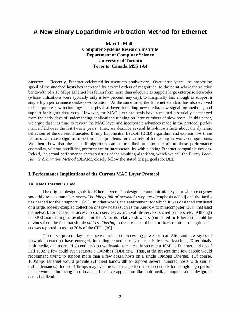
artificially generated traffic patterns were applied to the network to create a sustained overload situation.After a 5 second ‘‘warmup’’ period, each host then recorded its average throughput1 and channel accessdelays over a 10 second measurement interval.

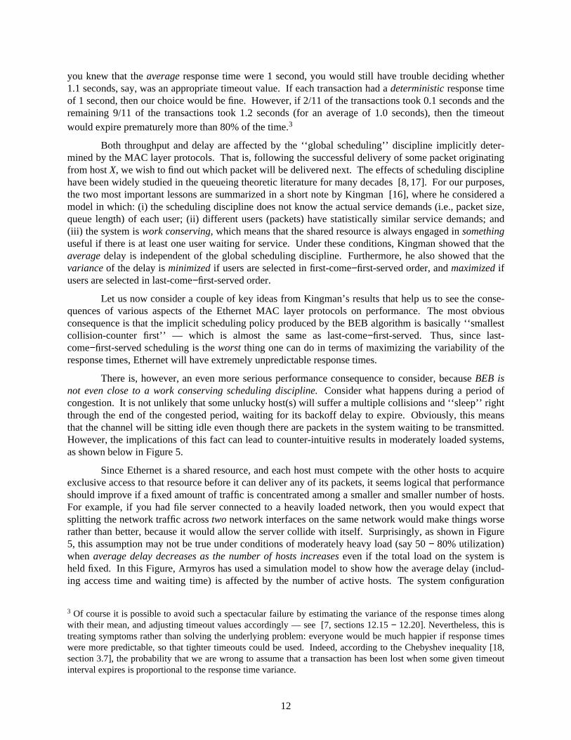
In Figure 1, we have reproduced many of the published Ethernet measurements from [6] for thecase of fixed-length packets. Notice that the maximum global throughput (in Mbits/sec.) reported foreach packet length occurred in a two-host system (a three-host system, in the case of 64 byte packets).This is because the DEC Titan workstations used in that study are quite slow by current standards: theauthors of [6] reported that the network controller in each host had to be reset by an interrupt routine(lasting approximately 100 µsec., or about two complete backoff slot-times) after each successful packettransmission. Clearly the Ethernet capture effect as described above could not have been a factor theirresults, since their hosts were far too slow to take advantage of it. Thus, we must find another explanationfor unexpectedly high capacity values reported in [6].

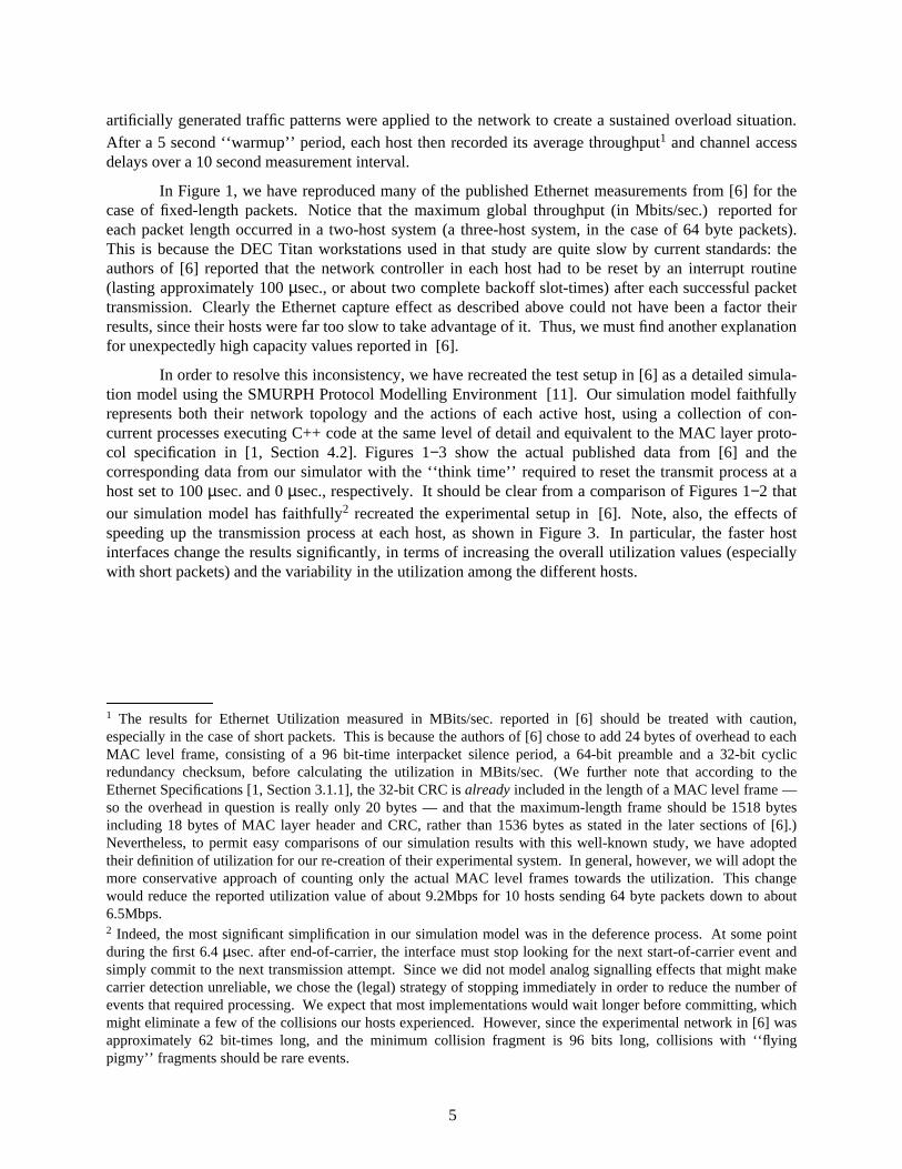
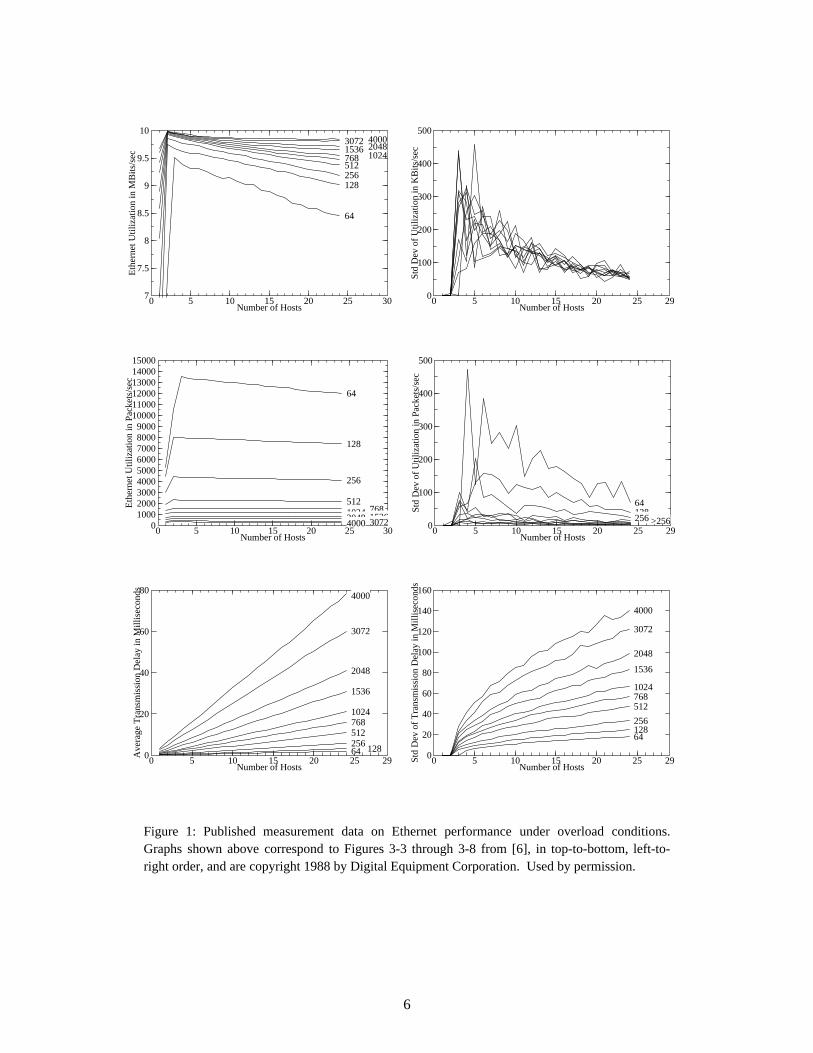
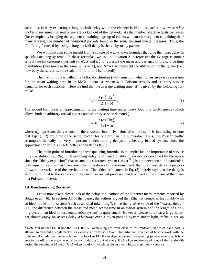
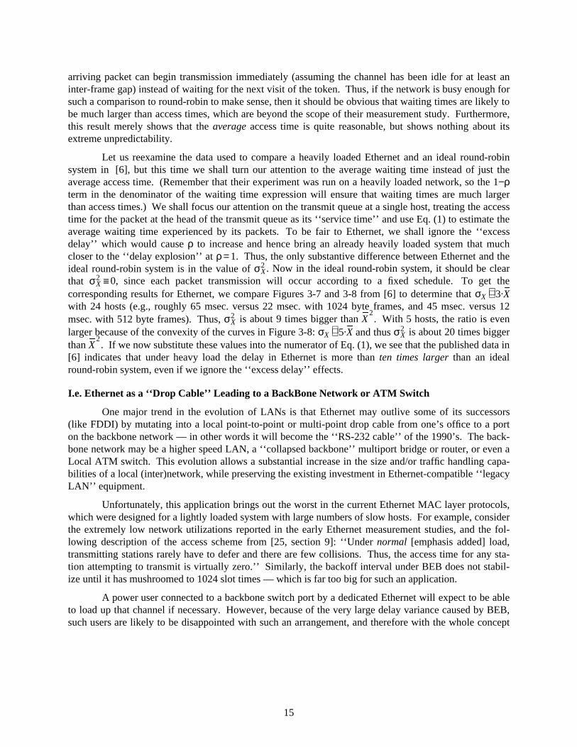
In order to resolve this inconsistency, we have recreated the test setup in [6] as a detailed simula-tion model using the SMURPH Protocol Modelling Environment [11]. Our simulation model faithfullyrepresents both their network topology and the actions of each active host, using a collection of con-current processes executing C++ code at the same level of detail and equivalent to the MAC layer proto-col specification in [1, Section 4.2]. Figures 1−3 show the actual published data from [6] and thecorresponding data from our simulator with the ‘‘think time’’ required to reset the transmit process at ahost set to 100 µsec. and 0 µsec., respectively. It should be clear from a comparison of Figures 1−2 thatour simulation model has faithfully2 recreated the experimental setup in [6]. Note, also, the effects ofspeeding up the transmission process at each host, as shown in Figure 3. In particular, the faster hostinterfaces change the results significantly, in terms of increasing the overall utilization values (especiallywith short packets) and the variability in the utilization among the different hosts.

� ��1 The results for Ethernet Utilization measured in MBits/sec. reported in [6] should be treated with caution,especially in the case of short packets. This is because the authors of [6] chose to add 24 bytes of overhead to eachMAC level frame, consisting of a 96 bit-time interpacket silence period, a 64-bit preamble and a 32-bit cyclicredundancy checksum, before calculating the utilization in MBits/sec. (We further note that according to theEthernet Specifications [1, Section 3.1.1], the 32-bit CRC is already included in the length of a MAC level frame —so the overhead in question is really only 20 bytes — and that the maximum-length frame should be 1518 bytesincluding 18 bytes of MAC layer header and CRC, rather than 1536 bytes as stated in the later sections of [6].)Nevertheless, to permit easy comparisons of our simulation results with this well-known study, we have adoptedtheir definition of utilization for our re-creation of their experimental system. In general, however, we will adopt themore conservative approach of counting only the actual MAC level frames towards the utilization. This changewould reduce the reported utilization value of about 9.2Mbps for 10 hosts sending 64 byte packets down to about6.5Mbps.2 Indeed, the most significant simplification in our simulation model was in the deference process. At some pointduring the first 6.4 µsec. after end-of-carrier, the interface must stop looking for the next start-of-carrier event andsimply commit to the next transmission attempt. Since we did not model analog signalling effects that might makecarrier detection unreliable, we chose the (legal) strategy of stopping immediately in order to reduce the number ofevents that required processing. We expect that most implementations would wait longer before committing, whichmight eliminate a few of the collisions our hosts experienced. However, since the experimental network in [6] wasapproximately 62 bit-times long, and the minimum collision fragment is 96 bits long, collisions with ‘‘flyingpigmy’’ fragments should be rare events.

5

0 305 10 15 20 25Number of Hosts

7

10

7.5

8

8.5

9

9.5

Eth

erne

t Util

izat

ion

in M

Bits

/sec

64

128256512768 10241536 20483072 4000


0

500

100

200

300

400

Std

Dev

of

Util

izat

ion

in K

Bits

/sec


0

15000

100020003000400050006000700080009000

1000011000120001300014000

Eth

erne

t Util

izat

ion

in P

acke

ts/s

ec

64

128

256

5127681024 15362048 30724000


0

500

100

200

300

400

Std

Dev

of

Util

izat

ion

in P

acke

ts/s

ec

64128256 >256


0

80

20

40

60

Ave

rage

Tra

nsm

issi

on D

elay

in M

illis

econ

ds

64 1282565127681024

1536

2048

3072

4000


0

160

20

40

60

80

100

120

140

Std

Dev

of

Tra

nsm

issi

on D

elay

in M

illis

econ

ds

64128256

5127681024

1536

2048

3072

4000

Figure 1: Published measurement data on Ethernet performance under overload conditions.Graphs shown above correspond to Figures 3-3 through 3-8 from [6], in top-to-bottom, left-to-right order, and are copyright 1988 by Digital Equipment Corporation. Used by permission.

6

7

7.5

8

8.5

9

9.5

10

0 5 10 15 20 25 29

Number of Hosts

Utilization

64

1282565127681024

1536204830724000

0

100

200

300

400

500

0 5 10 15 20 25 29

Number of Hosts

Util

Std

Dev

0

2000

4000

6000

8000

10000

12000

14000

0 5 10 15 20 25 29

Number of Hosts

Packets/Sec

64

128

256

51276810241536204830724000 0

100

200

300

400

500

0 5 10 15 20 25 29

Number of Hosts

Pkt/Sec

Std

Dev

6412825651276810241536204830724000

0

20

40

60

80

0 5 10 15 20 25 29

Number of Hosts

Trans

Delay

64128256512768

1024

1536

2048

3072

4000

0

20

40

60

80

100

120

140

160

180

200

0 5 10 15 20 25 29

Number of Hosts

Delay

Std

Dev

64128256

512768

1024

1536

2048

3072

4000

Figure 2: Reproduction of the data from Figure 1 via a detailed simulation model.

7

9

9.25

9.5

9.75

10

0 5 10 15 20 25 29

Number of Hosts

Utilization

64128

256

512

7681024

15362048

30724000

0

200

400

600

800

1000

0 5 10 15 20 25 29

Number of Hosts

Util

Std

Dev

0

2000

4000

6000

8000

10000

12000

14000

0 5 10 15 20 25 29

Number of Hosts

Packets/Sec

64

128

256

51276810241536204830724000 0

200

400

600

800

1000

0 5 10 15 20 25 29

Number of Hosts

Pkt/Sec

Std

Dev

6412825651276810241536204830724000

0

20

40

60

80

0 5 10 15 20 25 29

Number of Hosts

Trans

Delay

64128256512768

1024

1536

2048

3072

4000

0

20

40

60

80

100

120

140

160

0 5 10 15 20 25 29

Number of Hosts

Delay

Std

Dev 64

128256

512768

1024

1536

2048

3072

4000

Figure 3: Effect of reducing the time required to reset the transmit process to 0 in the simulation modelfrom Figure 2. (Notice the significant changes of scale in the bitwise utilization and both standard devia-tion of Utilization graphs.)

8

-0 2 4 6 8

0.0001

0.001

0.01

0.1

MRU Stack Depth

Acquisition

Prob

Host Reset Time = 100 µsec8 Hosts

64

128

2565127681024

153620483072

4000

-0 5 10 15 20 25

0.0001

0.001

0.01

0.1

MRU Stack Depth

Acquisition

Prob


64

128

2565127624

102415362042430724000

-0 2 4 6 8

0.0001

0.001

0.01

0.1

MRU Stack Depth

Acquisition

Prob


64

128

2565127681024

1536204830724000

-0 5 10 15 20 25

0.0001

0.001

0.01

0.1

MRU Stack Depth

Acquisition

Prob


64

128

2565127681024

1536204830724000

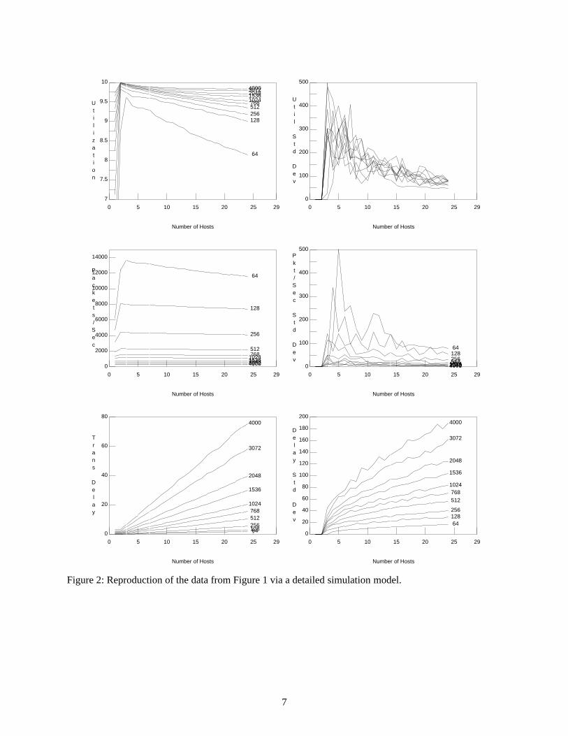
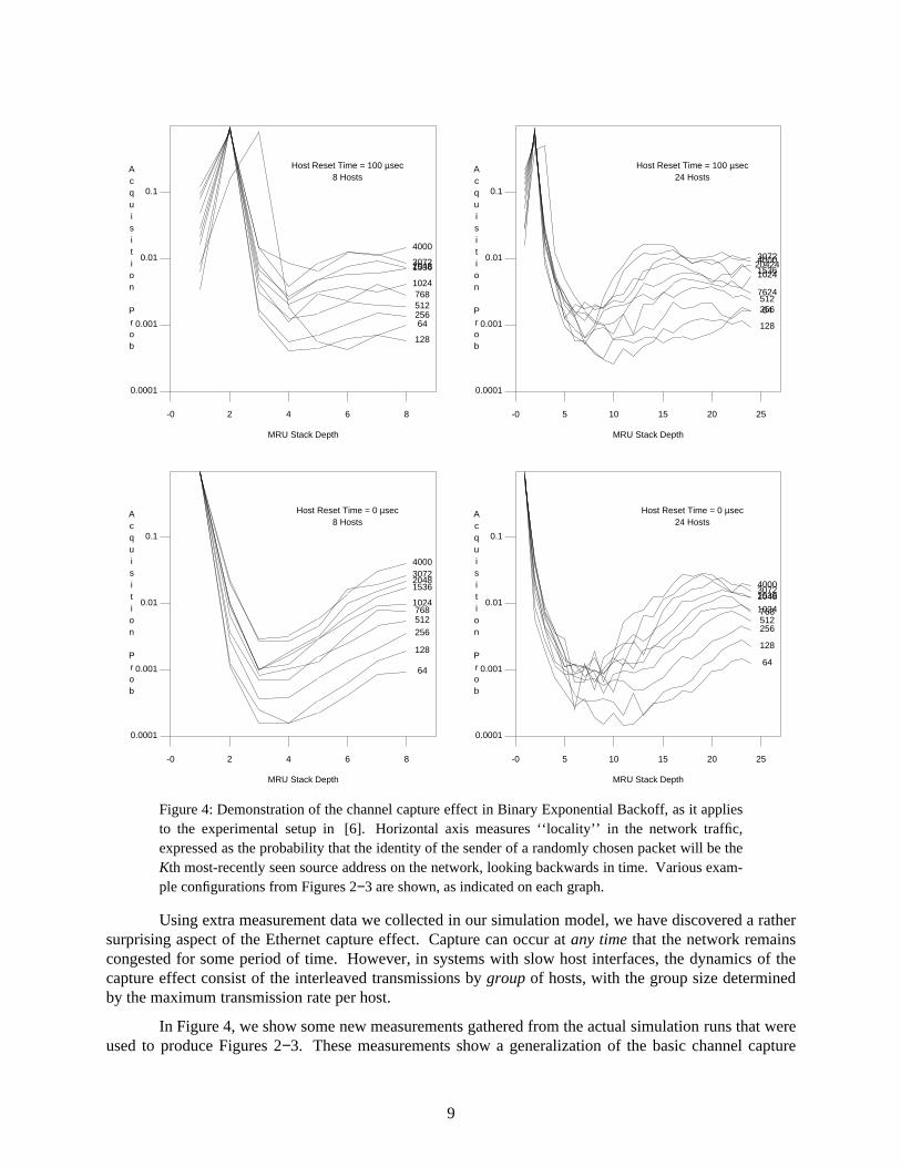
Figure 4: Demonstration of the channel capture effect in Binary Exponential Backoff, as it appliesto the experimental setup in [6]. Horizontal axis measures ‘‘locality’’ in the network traffic,expressed as the probability that the identity of the sender of a randomly chosen packet will be theKth most-recently seen source address on the network, looking backwards in time. Various exam-ple configurations from Figures 2−3 are shown, as indicated on each graph.

Using extra measurement data we collected in our simulation model, we have discovered a rathersurprising aspect of the Ethernet capture effect. Capture can occur at any time that the network remainscongested for some period of time. However, in systems with slow host interfaces, the dynamics of thecapture effect consist of the interleaved transmissions by group of hosts, with the group size determinedby the maximum transmission rate per host.

In Figure 4, we show some new measurements gathered from the actual simulation runs that wereused to produce Figures 2−3. These measurements show a generalization of the basic channel capture

9

idea, where one typically counts ‘‘run lengths’’ of consecutive packets with the same source address inthe output stream. In this Figure, however, we have adapted the concept of locality from the study ofpaged virtual memory systems to demonstrate that a group of slow hosts (such as the DEC Titan worksta-tions in [6]) is as effective as a single fast host at monopolizing the channel.

To produce this Figure, we maintained a list of host addresses sorted in Most Recently Used(MRU) order. That is, if we look at the list at any time t, then the host currently transmitting (or thattransmitted most recently, if the channel is currently idle) will be in position 1, the next most-recentlysuccessful host will be in position 2, and so on until the host whose most-recent packet transmission isfurthest in the past is at the end of the list. Each time a packet is sent, we increment a countercorresponding to the current position of the sending host in the MRU stack, and apply a cyclic shift tomove the sending host to the top of the stack. Thus, the data in this Figure shows the relation between thecurrent MRU stack depth for a host and the probability that it will acquire the network and transmit thenext packet. Notice that if there were no capture effect, then all hosts would be equally likely to send thenext packet, no matter which ones have been successful recently. Conversely, under complete capture bya single host (i.e., exhaustive service to an overloaded host), we would have probability 1.0 for the luckyhost at stack position 1, and 0.0 for all the rest.

Looking now at the actual data presented in Figure 4, it is interesting to note how unbalancedthese probabilities are — with those hosts that have transmitted recently (and hence are located near thetop of the MRU stack) being about 100 times more likely to acquire the channel than the others. Further-more, the effect of slowing the hosts to include a 100 µsec. reset time merely causes the capturing groupto expand from a single host to an alternating pair of hosts (a trio in the case of 64 byte packets), and hasvirtually no effect on the network acquisition probabilities for the hosts that are deeper in the MRU stack.It is interesting to note that in all 4 system configurations shown, the acquisition probability for hostsdeep in the MRU stack is a linear function of the packet length. Thus the data shows that in general, agiven host can capture the network for a specific amount of time, rather than for the transmission of aspecific number of packets — which is not surprising given that the time constants in BEB (which deter-mine how long the other hosts remain dormant) are independent of the packet size.

It is also interesting to compare the locality measure in our data with the predicted run lengthsusing the simple capacity model that we derived earlier. Consider the measured values of normalizedcapacity (including 24 bytes of MAC layer overhead per packet in the throughput calculation, asdescribed above) with 64-byte packets and either 8 or 24 active hosts, as reported by Boggs et al. [6].Using B = 88 bytes and the respective capacity values obtained from [6] into the capacity formula wederived above, we can solve the model to obtain an estimate of the average run length, which is approxi-mately 23 packets using the 8-host capacity value, or 10 packets using the 24 host capacity value. Thesefigures are remarkably close to the results we obtained from our source address locality measurements: ifwe consider references to the host at MRU stack depths 1 or 2 to be a continuation of the current ‘run’,then we can use the data from Figure 4 to estimate the average run lengths as approximately 25 packetsusing the 8-host stack reference data, or 15 packets using the 24-host stack reference data.

For comparison purposes, Tables 1−2 show the corresponding results for a more traditional meas-ure of the capture effect: the mean, standard deviation, and maximum ‘‘run lengths’’ observed duringsome of the experiments reported in Figures 2−3. While the magnitude of the run lengths in Table 2(with Host Reset Time = 0) is impressive, what is perhaps more important is the complete lack of evi-dence to show that the capture effect is taking place in Table 1 ( with Host Reset Time = 100 µsec.).Furthermore, by comparing the data in any column of Table 2, we can see that the channel holding timeby a single host is roughly inversely proportional to the number of active hosts.

10

� ��Packet Sizes� ��Hosts:

64 128 256 512 768 1024 1536 2048 3072 4000� �� 2 1 1 1 1 1 1 1 1 1 1

0 0 0 0 0 0 0 0 0 01 1 1 1 1 1 1 1 1 1� ��

4 1.002 1.002 1.002 1.006 1.009 1.014 1.019 1.031 1.037 1.048.0593 .0521 .0684 .1569 .1831 .2474 .2861 .4103 .4231 .5026

8 6 6 14 12 14 9 16 14 12 ��8 1.008 1.003 1.006 1.017 1.022 1.029 1.051 1.087 1.105 1.139

.1130 .0905 .1121 .2301 .2762 .3060 .4352 0.637 .7103 .840710 9 7 10 11 9 12 11 12 14 ��

16 1.020 1.009 1.017 1.040 1.060 1.076 1.112 1.156 1.204 1.222.1686 .1353 .1908 .3362 .4462 .5176 .6767 .8153 .9296 1.018

6 9 9 9 15 12 14 12 11 13� ��

��

��

��

��

��

��

��

��

��

��

��

��

Table 1: Measured run length statistics from the experiments used to create Figure 2, where theHost Reset Time = 100 µsec. Each entry consists of a triple, representing the mean, standarddeviation, and maximum run length observed in our re-creation of the experiments from [6]. Thedata shown provides no indication that the capture effect is present in this system. � � � � � � � � � � � � � � � � � � � � � � � � � � � � � � � � � � � � � � � � � � � � � � � � � � � � � � � � � � � � � � � � � � � � � � � � � � � � � � � � � � � � � � � � � � � � � � � � � � �

Packet Sizes��Hosts:64 128 256 512 768 1024 1536 2048 3072 4000��

2 2358 1064 800.0 331.8 239.0 190.7 116.1 113.1 72.89 57.061317 803.8 399.5 207.4 169.2 128.7 65.90 53.54 35.73 31.446010 2957 2169 875 679 492 219 249 166 141��

4 708.9 366.0 219.1 106.5 75.86 62.62 42.6 33.22 22.98 18.04654.6 382.7 209.1 114.7 72.96 58.07 40.30 33.34 22.22 16.57

2918 1486 771 441 354 243 158 129 118 72��8 250.8 165.2 86.12 50.78 33.45 25.22 18.79 15.39 10.23 8.31

324.4 208.6 106.6 59.42 37.48 28.97 19.04 15.51 10.52 7.961637 1258 582 319 194 163 86 72 50 46��

16 95.51 60.95 34.19 20.03 13.53 11.34 8.425 6.976 5.038 4.20147.2 84.16 49.29 26.95 17.66 13.56 9.54 7.758 5.181 3.928

1038 493 382 192 122 94 62 59 38 22��

��

��

��

��

��

��

��

��

��

��

��

��

Table 2: Measured run length statistics from the experiments used to create Figure 3, where HostReset Time = 0 µsec. This time, the run lengths clearly show the significance of the captureeffect.

I.c. Lessons from Queueing Theory: Making Users Happy

In any system involving a shared resource, one must be careful not to confuse the perceptions ofthe service provider with those of the users. In the case of a Local Area Network (like Ethernet), the pri-mary concern of the service provider is throughput, i.e., whenever there are packets in the system in needof transmission, the network should be engaged in delivering one of them. The users, on the other hand,are primarily concerned with delay, which consists of both access time (which measures the time that aparticular packet spends at the head of its own transmit queue) and waiting time (which measures the timeelapsed from the generation of a particular packet until its arrival at the head of the transmit queue).Furthermore, in many applications delay variance (also known as delay jitter ) is at least as important asaverage delay. It is well known that human users have a strong dislike for unpredictability in receivingthe results to an interactive request or the next segment of some continuous media like voice or video.Unpredictable response times also make it difficult to select suitable values for protocol timeouts: even if

11

you knew that the average response time were 1 second, you would still have trouble deciding whether1.1 seconds, say, was an appropriate timeout value. If each transaction had a deterministic response timeof 1 second, then our choice would be fine. However, if 2/11 of the transactions took 0.1 seconds and theremaining 9/11 of the transactions took 1.2 seconds (for an average of 1.0 seconds), then the timeoutwould expire prematurely more than 80% of the time.3

Both throughput and delay are affected by the ‘‘global scheduling’’ discipline implicitly deter-mined by the MAC layer protocols. That is, following the successful delivery of some packet originatingfrom host X, we wish to find out which packet will be delivered next. The effects of scheduling disciplinehave been widely studied in the queueing theoretic literature for many decades [8, 17]. For our purposes,the two most important lessons are summarized in a short note by Kingman [16], where he considered amodel in which: (i) the scheduling discipline does not know the actual service demands (i.e., packet size,queue length) of each user; (ii) different users (packets) have statistically similar service demands; and(iii) the system is work conserving, which means that the shared resource is always engaged in somethinguseful if there is at least one user waiting for service. Under these conditions, Kingman showed that theaverage delay is independent of the global scheduling discipline. Furthermore, he also showed that thevariance of the delay is minimized if users are selected in first-come−first-served order, and maximized ifusers are selected in last-come−first-served order.

Let us now consider a couple of key ideas from Kingman’s results that help us to see the conse-quences of various aspects of the Ethernet MAC layer protocols on performance. The most obviousconsequence is that the implicit scheduling policy produced by the BEB algorithm is basically ‘‘smallestcollision-counter first’’ — which is almost the same as last-come−first-served. Thus, since last-come−first-served scheduling is the worst thing one can do in terms of maximizing the variability of theresponse times, Ethernet will have extremely unpredictable response times.

There is, however, an even more serious performance consequence to consider, because BEB isnot even close to a work conserving scheduling discipline. Consider what happens during a period ofcongestion. It is not unlikely that some unlucky host(s) will suffer a multiple collisions and ‘‘sleep’’ rightthrough the end of the congested period, waiting for its backoff delay to expire. Obviously, this meansthat the channel will be sitting idle even though there are packets in the system waiting to be transmitted.However, the implications of this fact can lead to counter-intuitive results in moderately loaded systems,as shown below in Figure 5.

Since Ethernet is a shared resource, and each host must compete with the other hosts to acquireexclusive access to that resource before it can deliver any of its packets, it seems logical that performanceshould improve if a fixed amount of traffic is concentrated among a smaller and smaller number of hosts.For example, if you had file server connected to a heavily loaded network, then you would expect thatsplitting the network traffic across two network interfaces on the same network would make things worserather than better, because it would allow the server collide with itself. Surprisingly, as shown in Figure5, this assumption may not be true under conditions of moderately heavy load (say 50 − 80% utilization)when average delay decreases as the number of hosts increases even if the total load on the system isheld fixed. In this Figure, Armyros has used a simulation model to show how the average delay (includ-ing access time and waiting time) is affected by the number of active hosts. The system configuration

� ��3 Of course it is possible to avoid such a spectacular failure by estimating the variance of the response times alongwith their mean, and adjusting timeout values accordingly — see [7, sections 12.15 − 12.20]. Nevertheless, this istreating symptoms rather than solving the underlying problem: everyone would be much happier if response timeswere more predictable, so that tighter timeouts could be used. Indeed, according to the Chebyshev inequality [18,section 3.7], the probability that we are wrong to assume that a transaction has been lost when some given timeoutinterval expires is proportional to the response time variance.

12

0.0001

0.001

0.01

0.1

1

10

sec

Offered Load

Ethernet Response Time

0 0.1 0.2 0.3 0.4 0.5 0.6 0.7 0.8 0.9 1

..

..

..

..

..

..

..

..

..

..

..

..

..

..

..

..

..

..

..

..

..

..

..

..

..

..

..

..

..

..

.

5

10

2050100

0.2 0.4 0.6 0.8 1

10

100

frames

Offered Load

Mean # of frames in a row

..

..

..

..

..

..

..

..

..

..

..

..

..

..

..

..

..

..

..

..

..

..

..

..

..

..

..

..

..

..

.

2

3

5

10

20

50

100

Figure 5: Effect of Number of Active Hosts on Ethernet Response Times (including both waiting time andaccess time). Solid lines: simulation data by Armyros [5]. Dashed line: approximate analytical formula dueto Almes and Lazowska [4], which is based on the simplistic capacity analysis in [21]. Dotted line:predicted capacity using Almes and Lazowska’s formula, which ignores the capture effect.

used to produce this Figure is similar to the one reported by Boggs et al. [6], except that Armyros used abimodal packet length distribution (with 1/3 ‘‘short’’ 132 byte packets and 2/3 ‘‘long’’ 1096 byte pack-ets, for an average size of 775 bytes) and a symmetric Poisson arrival process at each host. From this Fig-ure, we can see three distinct ‘operating regimes’ at different throughput values. First, when thethroughput is less than about 5Mbps, the network is quiet. Here queueing delays are small compared tothe transmission time for a packet, and the simple analytical formula developed by Almes and Lazowska[4] is in good agreement with the simulation results, almost by default. The second region coversthroughput values between 5Mbps and 8Mbps, where the network is starting to get quite busy. Here thequeueing delays blow up suddenly, and we see an unusual inversion of the delay curves where the worstdelay performance comes with the fewest active hosts. Note also that the analytical delay formula isgrossly optimistic, to the point where the curve does not even exhibit the correct order of magnitude. Thefinal region covers throughput values in excess of 8Mbps, where the network is becoming saturated. Herethe delay inversion disappears and the capture effect takes over, allowing the throughput values to exceedthe maximum value predicted by the analytical formula by a substantial amount. It is interesting to notethe extent to which the capture effect can interfere with the short-term fairness of the protocol: as the net-work becomes completely saturated, each host in a 2-host system will on average transmit more than 100frames in a row before allowing the other one to send anything.4

The behaviour of the system when the network is either quiet or saturated is easy to understand.The anomalous behaviour in the middle region occurs because BEB is not even close to a work conserv-ing policy. Under these traffic conditions, the network is still somewhat starved for traffic. However, if

� ��4 Notice that in general, these run length numbers are in agreement with those in Table 2 for similar packet sizes(i.e., 768 byte), except for the 2-host system. We attribute this discrepancy to the fact that Armyros’ data isreporting an open system approaching saturation, whereas the data in Table 2 is for a closed system that is atsaturation.

13

some host is busy executing a long backoff delay while the channel is idle, that packet and every otherpacket in the same transmit queue are locked out of the network. As the number of active hosts decreases(for example, by bridging the segment containing a group of clients with another segment containing theirmain servers), the number of additional packets found in the same transmit queue increases. Thus, the‘‘suffering’’ caused by a single long backoff delay is shared by many packets.

We will also gain some insight from a couple of well-known formulas that give the mean delay inspecific queueing systems. In these formulas, we use the notation λ to represent the average customerarrival rate (in customers per unit time), X� � and σX

2 to represent the mean and variance of the service timedistribution (measured in the same units as λ), and ρ ≡ λ X� � to represent the utilization of the queue (i.e.,how busy the server is, on a scale of 0 [idle] to 1 [saturated]).

The first formula is called the Pollacek-Khinshin (P-K) equation, which gives an exact expressionfor the mean waiting time in an M/G/1 queue: a system with Poisson arrivals and arbitrary servicedemands for each customer. Here we find that the average waiting time, W�� , is given by the following for-mula:

W�� =2 (1 − ρ)

λ (σX2 + X� � 2

)� �� . (1)

The second formula is an approximation to the waiting time under heavy load in a G/G/1 queue (whichallows both an arbitrary arrival pattern and arbitrary service demands):

W!�! =2 (1 − ρ)

λ (σX2 + σλ

2 )"#"�"�"�"�"�"�"�"�" , (2)

where σλ2 represents the variance of the customer interarrival time distribution. It is interesting to note

that Eqs. (1−2) are almost the same, except for one term in the numerator. Thus, the Poisson trafficassumption is really not very important in determining delays in a heavily loaded system, since theapproximation in Eq. (2) gets better and better as ρ → 1.

The main point of introducing these queueing formulas is to emphasize the importance of servicetime variability (i.e., σX

2 ) in determining delay, and hence quality of service as perceived by the users,since the ‘‘delay explosion’’ that occurs in a saturated system (i.e., ρ ∼∼ 1) is not unexpected. In particular,both equations show that if we keep the utilization of the system fixed, then the mean delay is propor-tional to the variance of the service times. The added refinement in Eq. (2) merely says that the delay isalso proportional to the variance of the customer arrival process (which is fixed at the square of the meanin a Poisson process).

I.d. Benchmarking Revisited

Let us now take a closer look at the delay implications of the Ethernet measurements reported byBoggs et al. [6]. In section 3.5 of that paper, the authors argued that Ethernet compares favourably withan ideal round-robin system (such as an ideal token ring5), since the relative value of the ‘‘excess delay’’(i.e., the difference between the measured mean access time in an n-host system and the length of a pol-ling cycle in an ideal n-host round-robin system) is quite small. However, please note that a large Ether-net should enjoy an access delay advantage over a token-passing system under light traffic, since an

$ $�$�$�$�$�$�$�$�$�$�$�$�$�$5 Note that neither FDDI nor the IEEE 802.5 Token Ring are even close to this ‘‘ideal’’, in which each host isallowed to transmit a single packet for every visit by the idle token. In particular, given an M host network with theright initial conditions the timed-token protocol in FDDI can degenerate into a repeating pattern where each hostgets to use all of the asynchronous bandwith during 1 out of every M +1 token rotations and none of the bandwidthduring the remaining M out of M +1 token rotations, which results in a very high access delay variance.

14

arriving packet can begin transmission immediately (assuming the channel has been idle for at least aninter-frame gap) instead of waiting for the next visit of the token. Thus, if the network is busy enough forsuch a comparison to round-robin to make sense, then it should be obvious that waiting times are likely tobe much larger than access times, which are beyond the scope of their measurement study. Furthermore,this result merely shows that the average access time is quite reasonable, but shows nothing about itsextreme unpredictability.

Let us reexamine the data used to compare a heavily loaded Ethernet and an ideal round-robinsystem in [6], but this time we shall turn our attention to the average waiting time instead of just theaverage access time. (Remember that their experiment was run on a heavily loaded network, so the 1−ρterm in the denominator of the waiting time expression will ensure that waiting times are much largerthan access times.) We shall focus our attention on the transmit queue at a single host, treating the accesstime for the packet at the head of the transmit queue as its ‘‘service time’’ and use Eq. (1) to estimate theaverage waiting time experienced by its packets. To be fair to Ethernet, we shall ignore the ‘‘excessdelay’’ which would cause ρ to increase and hence bring an already heavily loaded system that muchcloser to the ‘‘delay explosion’’ at ρ = 1. Thus, the only substantive difference between Ethernet and theideal round-robin system is in the value of σX

2 . Now in the ideal round-robin system, it should be clearthat σX

2 ≡ 0, since each packet transmission will occur according to a fixed schedule. To get thecorresponding results for Ethernet, we compare Figures 3-7 and 3-8 from [6] to determine that σX ∼∼ 3.X% %with 24 hosts (e.g., roughly 65 msec. versus 22 msec. with 1024 byte frames, and 45 msec. versus 12msec. with 512 byte frames). Thus, σX

2 is about 9 times bigger than X& & 2. With 5 hosts, the ratio is even

larger because of the convexity of the curves in Figure 3-8: σX ∼∼ 5.X' ' and thus σX2 is about 20 times bigger

than X( ( 2. If we now substitute these values into the numerator of Eq. (1), we see that the published data in

[6] indicates that under heavy load the delay in Ethernet is more than ten times larger than an idealround-robin system, even if we ignore the ‘‘excess delay’’ effects.

I.e. Ethernet as a ‘‘Drop Cable’’ Leading to a BackBone Network or ATM Switch

One major trend in the evolution of LANs is that Ethernet may outlive some of its successors(like FDDI) by mutating into a local point-to-point or multi-point drop cable from one’s office to a porton the backbone network — in other words it will become the ‘‘RS-232 cable’’ of the 1990’s. The back-bone network may be a higher speed LAN, a ‘‘collapsed backbone’’ multiport bridge or router, or even aLocal ATM switch. This evolution allows a substantial increase in the size and/or traffic handling capa-bilities of a local (inter)network, while preserving the existing investment in Ethernet-compatible ‘‘legacyLAN’’ equipment.

Unfortunately, this application brings out the worst in the current Ethernet MAC layer protocols,which were designed for a lightly loaded system with large numbers of slow hosts. For example, considerthe extremely low network utilizations reported in the early Ethernet measurement studies, and the fol-lowing description of the access scheme from [25, section 9]: ‘‘Under normal [emphasis added] load,transmitting stations rarely have to defer and there are few collisions. Thus, the access time for any sta-tion attempting to transmit is virtually zero.’’ Similarly, the backoff interval under BEB does not stabil-ize until it has mushroomed to 1024 slot times — which is far too big for such an application.

A power user connected to a backbone switch port by a dedicated Ethernet will expect to be ableto load up that channel if necessary. However, because of the very large delay variance caused by BEB,such users are likely to be disappointed with such an arrangement, and therefore with the whole concept

15

of Ethernet connections to a backbone network.6

I.f. Predictable Performance is Worth Something

In spite of its dominance of the LAN market over the last decade, the merits and shortcomings ofEthernet remain a subject of intense religious debate. A large part of this controversy is caused by humannature: as with politics, people tend not to trust systems that they don’t understand. Right now, peoplereally don’t know how to evaluate the performance of their Ethernet, and even simple questions like:

i. How many hosts can be supported by one network? or

ii. How much traffic can be supported by one network? or

iii. How many collisions is acceptable?

do not have understandable, widely accepted answers — the way we have ‘rules of thumb’ to say that theutilization of a statistical multiplexer should not exceed 80% [27, section 2.4.6]. Thus, rumours spreadthat Ethernet cannot do X, or that some other technology (say token rings) are better for Y.

Furthermore, even the most determined performance analysts will get discouraged when theyrealize that the delay, say, depends on so many details in addition to the obvious ones of total traffic andnumber of hosts. In particular, the exact topology (which affects propagation delays) and the exact timingof the traffic generated by each host (which together with topology determines the likelihood of colli-sions) and the history of channel activity over the last several seconds (which affects the queue lengthsand collision counter values at each host) also have a significant influence. When you then pile on theeffects of the message generation patterns of the major applications being run at each host, the timeoutupdate algorithms being used by the transport layer protocols, and the capabilities of the network inter-face, it is tempting to simply give up on performance prediction and claim that Ethernet is some kind ofchaotic system.

After having spent considerable effort myself in trying to understand Ethernet performance overmany years, I have finally reached the following conclusions. First, it was a mistake to call the MAClayer protocol ‘‘CSMA/CD’’, since the real key to understanding its performance lies in capturing theessence of the BEB algorithm. Indeed, in [26] we developed the best currently available formula7 relat-ing throughput, S, to the total transmission attempt rate, G, for unslotted 1-persistent CSMA/CD — but itis almost useless for modelling Ethernet (where we would like to be able to predict the average number ofcollisions per packet, (G −S)/S, as a function of system load, S) because of the strong influence of BEB onthe short-term traffic patterns.

) )�)�)�)�)�)�)�)�)�)�)�)�)�)6 For certain media, this worst-case MAC-layer performance when Ethernet is used as a point-to-point cable from aworkstation to a backbone switch port can be avoided using the proposed ‘‘Full Duplex’’ modification. If thephysical layer consists of a pair of unidirectional point-to-point channels (such as twisted pair or an optical fiber),then by disabling the collision detection and loopback circuitry at each end we can treat the network as a pair ofindependent, collision-free unidirectional channels connecting the transmit circuit on one end to the receive circuitat the other end. However, this solution does not work for any system with more than two devices per collisiondomain, for systems using coaxial cable, or for 100BaseT4 systems (which use 3 out of 4 wire pairs in parallel tosend the data in a single direction).7 The reader who is familiar with the brief guide to the theoretical studies in [6] may notice that our paper was notincluded, which is unfortunate because our paper corrected a serious error in the mathematical model of Takagi andKleinrock [28], which was discussed in section 2.4.6. The correct throughput curve does not have the peculiardouble-peaked shape, nor is the maximum throughput limited to 50% even in the zero propagation delay limit —both of which were obviously wrong given the measured throughput data presented in [6].

16

The second conclusion is that it is unlikely that a more accurate analytical model can be foundeven if we ignore the state of the host and its transmit queue size. Just describing the combined state ofthe network interfaces for all active hosts leads to a combinatorial explosion: at each end-of-carrier event,we cannot determine what will happen next without knowing both the collision counter value and theremaining time until the current backoff delay (if any) expires for each host [33]. Any progress onfinding a suitable model will depend on simplifying the allowable set of states at each end-of-carrierevent. The coordinated updates to the backoff counters in the Binary Logarithmic Arbitration Methodprovide just such a state reduction, and hence the possibility of a performance model that is both tractableand accurate.

II. It Wasn’t Supposed to Work This Way

II.a. Binary ‘‘Exponential’’ Backoff is Really a Linear Search for Q

Most people don’t understand the intricacies of Ethernet’s Truncated Binary Exponential Backoff(BEB) algorithm. Obviously, the backoff delay intervals selected by a given host increase exponentiallywith the number of collisions. It is also easy to see that an unlucky host that fails to acquire the Etherafter several attempts is doomed to suffer a very large and unpredictable network access delay. However,although no such claim appears in the original Metcalfe and Boggs CACM paper [21], most Ethernetusers seem willing to accept this draconian treatment of the oldest packets in the the system, because theybelieve it allows BEB to defuse ‘‘collision storms’’ exponentially quickly. Unfortunately, as we shallnow see, BEB is really just a linear algorithm in terms of its reaction time to a transient overload situa-tion. Thus, it is actually rather slow at adapting to transient overload conditions.

For illustrative purposes, let us assume that the cost of each collision is simply one backoff slottime (or 512 bits), so we can determine the running time for the algorithm by counting slot times, ratherthan getting bogged down in event timing [26] and/or geometric [23] details. Note that each collisionincludes a 96 bit-time inter-packet space and between 96 and about 570 bit times of activity,8 i.e., thetotal cost of a collision is roughly 3/8 to 4/3 backoff slot times, so this equal cost assumption will be pes-simistic in most cases.

Now consider the unhappy situation that would arise if some event triggered a large number ofhosts to start transmitting simultaneously. (The possibility of such broadcast storms is well known to net-work administrators, for example, they can be triggered by configuration errors that cause multiple hoststo attempt to forward broadcasts. They would become routine events if another proposal to ‘‘solve’’ thecapture effect were adopted in which the backoff algorithm for all hosts was reset after every successfultransmission.) Near the time of such a ‘‘Big Bang’’, it should be obvious that if the number of activehosts is large, none of their early transmission attempts has any hope of succeeding. We can use this fact,together with the simplified initial conditions implied by the ‘‘Big Bang’’ to determine the average timeuntil the first successful packet transmission occurs in such a system.

First, we need to determine the probability Pn that a particular host will make another transmis-sion attempt at the nth time step, given that nobody has been successful during the first n −1 steps. Now,recall that under BEB, the starting time for the next attempt will be randomly selected from the next2min (c, 10) slots, where c counts the number of previous attempts for this packet. Thus, it should be clearthat our particular host must select slot 1 for its first attempt, and thereafter it may select slot n for itsc +1st attempt only if it selected one of slots n −1, n −2, . . . , n −2min(c, 10) for its cth attempt. Thus, we can

* *�*�*�*�*�*�*�*�*�*�*�*�*�*8 The lower bound comes from the fact that the 32-bit jam cannot begin until a complete 64-bit preamble has beensent; the upper bound comes from a worst-case timing analysis for collisions, described in Appendix A1.3 of theEthernet Specification [1].

17

determine {Pn} using the equations:

Pn =c =0Σ15

Pn(c) (3)

where Pn(c) is the probability that a particular host makes its c +1st attempt in slot n, given that nobodyhas successfully acquired the channel during the first n −1 steps, and Pn(c) is determined by the followingset of recursive equations:

Pn(c) =k =max(1, n −210)

Σn −1

210

Pk(c −1)+ +�+�+�+�+�+�+Pn(c) =

k =max(1, n −2c)Σn −1

2c

Pk(c −1), ,�,�,�,�,�,�,Pn(0) = Pn −1(15)

P 1(0) = 1, P 1(c) = 0

n > 1, c ≥ 10

n > 1, c < 10

n > 1

c > 0

(4)

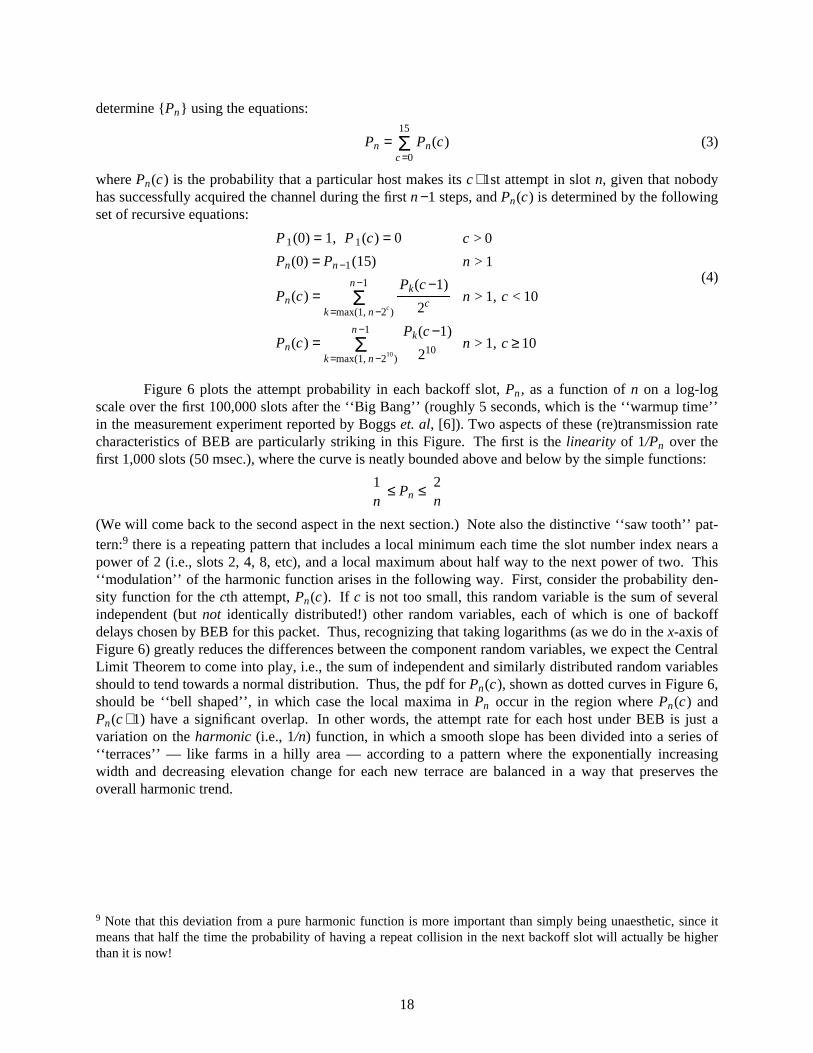
Figure 6 plots the attempt probability in each backoff slot, Pn , as a function of n on a log-logscale over the first 100,000 slots after the ‘‘Big Bang’’ (roughly 5 seconds, which is the ‘‘warmup time’’in the measurement experiment reported by Boggs et. al, [6]). Two aspects of these (re)transmission ratecharacteristics of BEB are particularly striking in this Figure. The first is the linearity of 1/Pn over thefirst 1,000 slots (50 msec.), where the curve is neatly bounded above and below by the simple functions:

n1-.- ≤ Pn ≤

n2/./

(We will come back to the second aspect in the next section.) Note also the distinctive ‘‘saw tooth’’ pat-tern:9 there is a repeating pattern that includes a local minimum each time the slot number index nears apower of 2 (i.e., slots 2, 4, 8, etc), and a local maximum about half way to the next power of two. This‘‘modulation’’ of the harmonic function arises in the following way. First, consider the probability den-sity function for the cth attempt, Pn(c). If c is not too small, this random variable is the sum of severalindependent (but not identically distributed!) other random variables, each of which is one of backoffdelays chosen by BEB for this packet. Thus, recognizing that taking logarithms (as we do in the x-axis ofFigure 6) greatly reduces the differences between the component random variables, we expect the CentralLimit Theorem to come into play, i.e., the sum of independent and similarly distributed random variablesshould to tend towards a normal distribution. Thus, the pdf for Pn(c), shown as dotted curves in Figure 6,should be ‘‘bell shaped’’, in which case the local maxima in Pn occur in the region where Pn(c) andPn(c +1) have a significant overlap. In other words, the attempt rate for each host under BEB is just avariation on the harmonic (i.e., 1/n) function, in which a smooth slope has been divided into a series of‘‘terraces’’ — like farms in a hilly area — according to a pattern where the exponentially increasingwidth and decreasing elevation change for each new terrace are balanced in a way that preserves theoverall harmonic trend.

0 0�0�0�0�0�0�0�0�0�0�0�0�0�09 Note that this deviation from a pure harmonic function is more important than simply being unaesthetic, since itmeans that half the time the probability of having a repeat collision in the next backoff slot will actually be higherthan it is now!

18

0.001

0.01

0.1

1.0

1 10 100 1,000 10,000 100,000

Contention Slot Number, n

Pn

................. .. .. .. .. ..

..............

........................ ..

... ..........................

...................................

. . ............

......................

.................................

.. .. . . ...................................

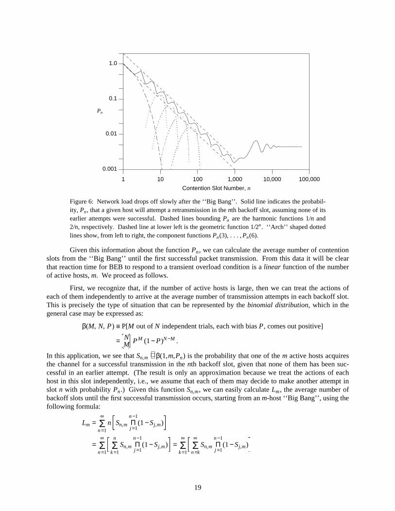
Figure 6: Network load drops off slowly after the ‘‘Big Bang’’. Solid line indicates the probabil-ity, Pn, that a given host will attempt a retransmission in the nth backoff slot, assuming none of itsearlier attempts were successful. Dashed lines bounding Pn are the harmonic functions 1/n and2/n, respectively. Dashed line at lower left is the geometric function 1/2n. ‘‘Arch’’ shaped dottedlines show, from left to right, the component functions Pn(3), . . . , Pn(6).

Given this information about the function Pn , we can calculate the average number of contentionslots from the ‘‘Big Bang’’ until the first successful packet transmission. From this data it will be clearthat reaction time for BEB to respond to a transient overload condition is a linear function of the numberof active hosts, m. We proceed as follows.

First, we recognize that, if the number of active hosts is large, then we can treat the actions ofeach of them independently to arrive at the average number of transmission attempts in each backoff slot.This is precisely the type of situation that can be represented by the binomial distribution, which in thegeneral case may be expressed as:

β(M, N, P) ≡ P[M out of N independent trials, each with bias P , comes out positive]

=12MN34 P M (1 − P)N −M .

In this application, we see that Sn,m ∼∼ β(1,m,Pn) is the probability that one of the m active hosts acquiresthe channel for a successful transmission in the nth backoff slot, given that none of them has been suc-cessful in an earlier attempt. (The result is only an approximation because we treat the actions of eachhost in this slot independently, i.e., we assume that each of them may decide to make another attempt inslot n with probability Pn .) Given this function Sn,m , we can easily calculate Lm , the average number ofbackoff slots until the first successful transmission occurs, starting from an m-host ‘‘Big Bang’’, using thefollowing formula:

Lm =n =1Σ∞

n56Sn,m

j =1Π

n −1(1 − Sj,m)

78

=n =1Σ∞ 9:

k =1Σn

Sn,mj =1Π

n −1(1 − Sj,m)

;<=

k =1Σ∞ =>

n =kΣ∞

Sn,mj =1Π

n −1(1 − Sj,m)

?@

19

=k =1Σ∞ AB

j =1Π

k −1(1 − Sj,m)

CD≡

k =1Σ∞

Fk −1 , (5)

where F 0 = 1, and Fk = (1−Sk,m).Fk −1 for all k >0, represents the probability that all hosts have failed toacquire the network during the first k backoff slot times. Since the function Fk is decreasing at leastgeometrically fast as k increases, Lm is easy to evaluate despite the infinite summation. Figure 7 shows aplot of Lm as a function of m. Also shown is the sample mean obtained by Monte Carlo simulation,where we have repeated the m-host ‘‘Big Bang’’ experiment until the width of the 95% confidence inter-val is below 4% of the mean. Notice the excellent agreement between Eq. (5) and the simulation data,especially for m ≥4, which shows that the independence assumption is not very important. Note also thatLm is growing linearly with the number of active of hosts, m, with Lm ∼∼ 2/9.m when m >> 1.

1

2

5

10

20

50

100

200

500

1 2 5 10 20 50 100 200 500 1000

Number of Active Hosts, m

Reaction

Ti

me

Lm . . . . . . . . . .. . . . . .. . . .. . . .. . . . .. . . . .. . . . . .. . . .. . . . . .. . . . . . .. . . . .. . . . .. . . . . .. . . .. . . . . .. . . . . . .. . . . .. . . . .

Figure 7: Average time to the first successful transmission after the ‘‘Big Bang’’, starting from mactive hosts. Solid line is from Eq. (5), which is approximate because of an independenceassumption. Dashed line is the sample mean obtained by Monte Carlo simulation of the exact sys-tem. Dotted line is from Eq. (6), which is the equivalent result for the Binary Logarithmic Arbi-tration Method that will be introduced in section III.

II.b. BEB is Supposed to be Stable for up to 1024 Hosts, but Isn’t

Another aspect of Figure 6 worth noting is the convergence to steady-state after the 1000th slottime, as the possibility that the collision counter has ‘‘wrapped around’’ after 16 unsuccessful attemptsbecomes more significant. In particular, the pattern of damped oscillations has completely decayed tozero in less than 1 second, at which point the steady-state probability that the given host transmits in eachbackoff slot is approximately10 1/225. This result means that Ethernet using BEB will become bistable if

E E�E�E�E�E�E�E�E�E�E�E�E�E�E10 We can calculate its exact value quite easily using the following argument. The first attempt for a new packettakes exactly 1 slot, the second attempt is equally likely to take 1 or 2 slots, and so on, so the average time until wehit an excessive collision error at the end of the 16th attempt is:

1 +2

1 + 2F F�F�F�F +4

1 + 2 + 3 + 4GHG�G�G�G�G�G�G�G�G . . . + 6 ×1024

1 + 2 + . . . + 1024I�I�I�I�I�I�I�I�I�I�I�I�I�I�I = 1 +23JKJ +

25LKL +

29MKM + . . . +

2513NKN�N�N + 6 ×

21025OKO�O�O�O =

213 + 7 ×1024P#P�P�P�P�P�P�P�P�P�P .

Thus, recognizing that a given host makes 16 transmission attempts over such a ‘‘cycle’’, we see that in steady stateits contribution to the channel traffic is (13 + 7 ×1024) / 32 = 1/224.4 transmission attempts per slot time. It is also

20

the number of hosts in a single collision domain is significantly larger than 225, and in particular thatanything approaching 1024 hosts will be problematic. Thus, if a situation ever arose in such a systemwhere most of the hosts were trying to transmit packets at the same time, there is a chance that the systemcould enter the ‘‘steady state’’ operating mode, where each host independently cycles around itsbackoff/retry loop, generating an average of 1 packet every 225 slot times. If the number of hosts is muchlarger than 225, then almost every attempt will end in another collision and the system will remain in thisdegraded operating mode for a very long time. Note that bistable behaviour does not necessarily meanthat the system, when started from a ‘‘good’’ state (like all hosts quiet), will not work at all. It simplymeans that eventually it will move from its ‘‘good’’ operating mode to its ‘‘bad’’ one, and possibly backagain. The time spent in the ‘‘good’’ operating mode depends on such factors as average load on the sys-tem and detailed topology and traffic information, which is beyond the scope of this paper. However, it isimportant to note that the operation of the system during the ‘‘bad’’ operating mode does not depend ondetailed traffic patterns: as long as each host’s transmit queue remains non-empty, its future transmissiontimes are completely determined by the MAC layer protocol. And in particular, since BEB is a discretetime algorithm, synchronizing the transmissions by different hosts to some integer multiple of a slot timebeyond end-of-carrier, even topology is of minor importance in an overload situation.

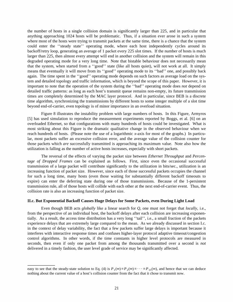
Figure 8 illustrates the instability problem with large numbers of hosts. In this Figure, Armyros[5] has used simulation to reproduce the measurement experiments reported by Boggs, et al. [6] on anoverloaded Ethernet, so that configurations with many hundreds of hosts could be investigated. What ismost striking about this Figure is the dramatic qualitative change in the observed behaviour when wereach hundreds of hosts. (Please note the use of a logarithmic x-axis for most of the graphs.) In particu-lar, most packets suffer an excessive collision error, and the average value of the collision counter forthose packets which are successfully transmitted is approaching its maximum value. Note also how theutilization is falling as the number of active hosts increases, especially with short packets.

The reversal of the effects of varying the packet size between Ethernet Throughput and Percen-tage of Dropped Frames can be explained as follows. First, since even the occasional successfultransmission of a large packet will contribute significantly to the utilization in bits/sec., utilization is anincreasing function of packet size. However, since each of those successful packets occupies the channelfor such a long time, many hosts (even those waiting for substantially different backoff timeouts toexpire) can enter the deferring state during one of those transmissions. Because of the 1-persistenttransmission rule, all of those hosts will collide with each other at the next end-of-carrier event. Thus, thecollision rate is also an increasing function of packet size.

II.c. But Exponential Backoff Causes Huge Delays for Some Packets, even During Light Load

Even though BEB acts globally like a linear search for Q, one must not forget that locally, i.e.,from the perspective of an individual host, the backoff delays after each collision are increasing exponen-tially. As a result, the access time distribution has a very long ‘‘tail’’, i.e., a small fraction of the packetsexperience delays that are extremely large compared to the mean. As we already discussed in section I.c.in the context of delay variability, the fact that a few packets suffer large delays is important because itinterferes with interactive response times and confuses higher-layer protocol adaptive timeout/congestioncontrol algorithms. In other words, if the time constants in higher level protocols are measured inseconds, then even if only one packet from among the thousands transmitted over a second is notdelivered in a timely fashion, the user level grade of service may be significantly affected.

Q Q�Q�Q�Q�Q�Q�Q�Q�Q�Q�Q�Q�Q�Qeasy to see that the steady-state solution to Eq. (4) is P 1(∞) = P 2(∞) = . . . = P 15(∞), and hence that we can deducenothing about the current value of a host’s collision counter from the fact that it chose to transmit now.

21

0 100 200 300 400

0.001

0.01

0.1

sec

Ethernet Transmission Delay

Number of Hosts

.

.

.

...

...

.........................

....

.... . . . .. . . . .. . . .. . . .. . . .. . . .. . . .. . . .. . . .. .. . .. . . .. . . .. . . .. . . .. . . .

.

..

.

...

....................

....

.. . . . .. . . . .. . . .. . . .. . . .. . . .. . . .. . . .. . . .. . . .. . . .

..

..

...

..

....................

.....

. . . .. . . . .. . . .. . . .. . . .. . . .. . . .

64128256

5121024

20483072

4000

1 10 100

4e+06

6e+06

8e+06

1e+07

bits/sec

Number of Hosts

Ethernet Throughput

.................... . . . .. . . .. . .. . .. .. .. .. .. .. .. .. ......... . . . . . . .. . . . .. . . .. . .. . .. .. .. .. .. .... .............

. .. . .

. . ... . . . .. . . . . . . . . . . . . . . . . . .. . . . . . .. . . . .. . . .. . .. . .. .. .. .. .. .. .. .

. . . . . . . .. . . . .. . . . . . . . . . . . . . . . . . .. . . . . . .. . . . .. . . .. . .. . .. .. .. .

64

128

256

512

1024

20483072

4000

1 10 100

0

20

40

60

80

%

Number of Hosts

Percentage of Dropped Frames

. . . . . . .. . . . .. . . .. . .. . .. .. .. .. .. .. .. ............ . . . . . . .. . . . ...

.... .

.....

...........

.......................

. . . . . . .. . . . .. . . .. . .. . .. .. .. .. .. .. .. ..............

...... .

. .. .

. .. ..

....

.....

.....

..................

..................

.

R R. . . . . . . S. . . . . T. . . . U. . . V. . . W. . X. . Y. . Z. . [. . \. . ]. . ^.. _.. `.. a.. b..c..d.. e..f..g..h..i..

j..

....

....

..

k..

....

..

l....... m..

... n..

.. o.... p..

. q... r... s. .t..u.. v. . w. . x.. y..

× × × × × × ×××××××××

×××××

×××××

×

×

×

××

×××××××

××××

......................................

............z

....

.

+ +. . . . . . .+

. . . . .

+

....

....

....

....

....

....

....

....

+

..............

+

....

....

+..

...

+. .

..+

. . . +. ..+...+.

.+. .+. .+. .+. .

. . . . . . .. .. .

. ....

....

....

....

....

....

....

....

....

................

....

.... .

.... .

.. . .. . .... .

64

2564000

128. . . . . . .{ { 512

×× 1024. . . . . . .++ 2048

3076. . . . . . . 64,256,4000

1 10 100

0

5

10

15

times

Number of Hosts

Retransmissions per frame

. . . . . . .. . . . .. . . .. . .. . .. .. .. .. .. .. .. .. .............

. . . . .. . . ..

. .. .

.....

.....

......

............

..................

. . . . . . .. . . . .. . . .. . .. . .. . .... .. .. .. .. .. ..

............

............

....

.....

....

.....

.....

.....

........

......

........

.. ......

.

|. . . . . . .}. . . . .~. . . .�. . .�. . .�. . .�. .�. .�. .�. .�. .�. .�. .�..�..�..�..�..�..�..�..�..�..�..�.....

....

...�.......

.�......�....

.�....�. . .�...�...�. .�. .� �..�. . . .¡..¢..£

× ××

××

××××××××

××××

×××××

×××

×

×

××

×××××××××

×××

.....

............................

........

... . .¤

+ +. . . . . . .

+. .

. .. .

+

....

....

....

....

....

....

....

....

.

+

....

....

....

.

+

....

...

+..

...

+..

..+. . . +. . .

+. .+. .+. .+. .+. .+. .

. . . . . . .....

.....

....

....

....

....

....

....

....

....

.....

....

....

.....

.....

... ..

. .... .. . ..

.. .

64

256

4000128

. . . . . . .¥ ¥ 512× × 1024. . . . . . .+ + 2048

3076. . . . . . . 64,256,4000

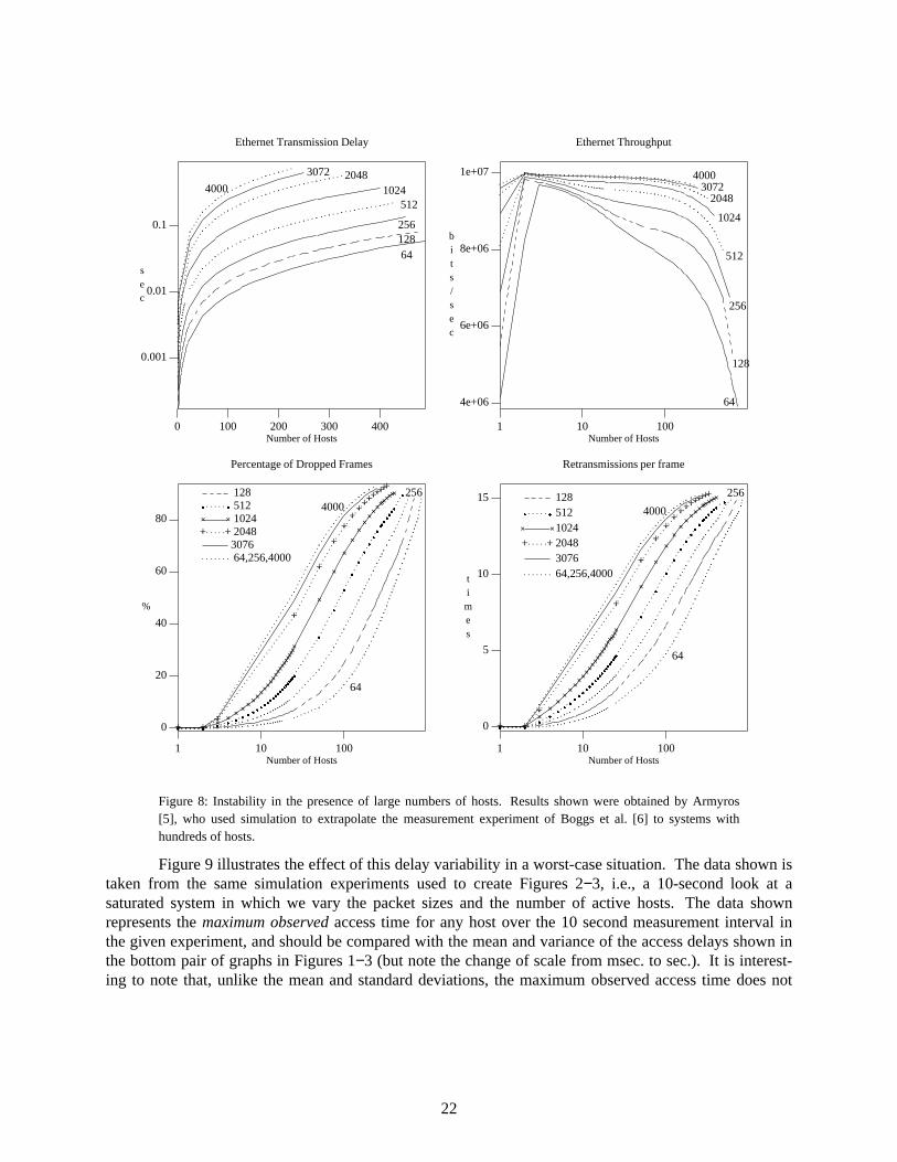
Figure 8: Instability in the presence of large numbers of hosts. Results shown were obtained by Armyros[5], who used simulation to extrapolate the measurement experiment of Boggs et al. [6] to systems withhundreds of hosts.

Figure 9 illustrates the effect of this delay variability in a worst-case situation. The data shown istaken from the same simulation experiments used to create Figures 2−3, i.e., a 10-second look at asaturated system in which we vary the packet sizes and the number of active hosts. The data shownrepresents the maximum observed access time for any host over the 10 second measurement interval inthe given experiment, and should be compared with the mean and variance of the access delays shown inthe bottom pair of graphs in Figures 1−3 (but note the change of scale from msec. to sec.). It is interest-ing to note that, unlike the mean and standard deviations, the maximum observed access time does not

22

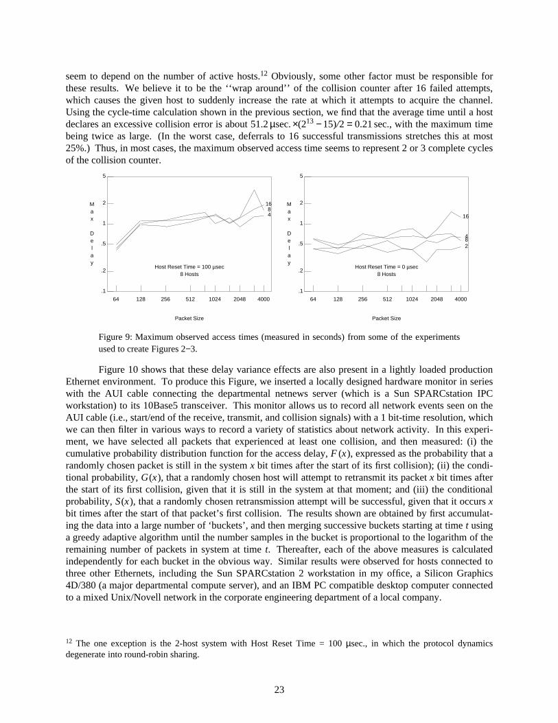
seem to depend on the number of active hosts.12 Obviously, some other factor must be responsible forthese results. We believe it to be the ‘‘wrap around’’ of the collision counter after 16 failed attempts,which causes the given host to suddenly increase the rate at which it attempts to acquire the channel.Using the cycle-time calculation shown in the previous section, we find that the average time until a hostdeclares an excessive collision error is about 51.2 µsec. ×(213 − 15)/2 = 0.21 sec., with the maximum timebeing twice as large. (In the worst case, deferrals to 16 successful transmissions stretches this at most25%.) Thus, in most cases, the maximum observed access time seems to represent 2 or 3 complete cyclesof the collision counter.

64 128 256 512 1024 2048 4000

.1

.2

.5

1

2

5

Packet Size

Max

Delay


48

16

64 128 256 512 1024 2048 4000

.1

.2

.5

1

2

5

Packet Size

Max

Delay


2

48

16

Figure 9: Maximum observed access times (measured in seconds) from some of the experimentsused to create Figures 2−3.

Figure 10 shows that these delay variance effects are also present in a lightly loaded productionEthernet environment. To produce this Figure, we inserted a locally designed hardware monitor in serieswith the AUI cable connecting the departmental netnews server (which is a Sun SPARCstation IPCworkstation) to its 10Base5 transceiver. This monitor allows us to record all network events seen on theAUI cable (i.e., start/end of the receive, transmit, and collision signals) with a 1 bit-time resolution, whichwe can then filter in various ways to record a variety of statistics about network activity. In this experi-ment, we have selected all packets that experienced at least one collision, and then measured: (i) thecumulative probability distribution function for the access delay, F (x), expressed as the probability that arandomly chosen packet is still in the system x bit times after the start of its first collision); (ii) the condi-tional probability, G(x), that a randomly chosen host will attempt to retransmit its packet x bit times afterthe start of its first collision, given that it is still in the system at that moment; and (iii) the conditionalprobability, S(x), that a randomly chosen retransmission attempt will be successful, given that it occurs xbit times after the start of that packet’s first collision. The results shown are obtained by first accumulat-ing the data into a large number of ‘buckets’, and then merging successive buckets starting at time t usinga greedy adaptive algorithm until the number samples in the bucket is proportional to the logarithm of theremaining number of packets in system at time t. Thereafter, each of the above measures is calculatedindependently for each bucket in the obvious way. Similar results were observed for hosts connected tothree other Ethernets, including the Sun SPARCstation 2 workstation in my office, a Silicon Graphics4D/380 (a major departmental compute server), and an IBM PC compatible desktop computer connectedto a mixed Unix/Novell network in the corporate engineering department of a local company.

¦ ¦�¦�¦�¦�¦�¦�¦�¦�¦�¦�¦�¦�¦�¦12 The one exception is the 2-host system with Host Reset Time = 100 µsec., in which the protocol dynamicsdegenerate into round-robin sharing.

23

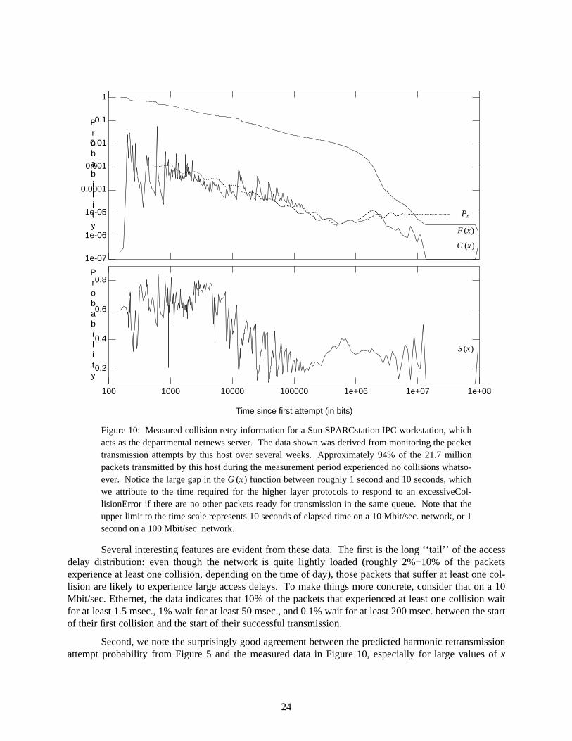
1

0.1

0.01

0.001

0.0001

1e-05

1e-06

1e-07

Probability

F (x)

G (x)

........................................... .................. ........ . ........................................................................ .......................... .......................... .................................. ....

............

.. .................................... .............. ...................................................... Pn

Time since first attempt (in bits)

Probability

100 1000 10000 100000 1e+06 1e+07 1e+08

0.2

0.4

0.6

0.8

S (x)

Figure 10: Measured collision retry information for a Sun SPARCstation IPC workstation, whichacts as the departmental netnews server. The data shown was derived from monitoring the packettransmission attempts by this host over several weeks. Approximately 94% of the 21.7 millionpackets transmitted by this host during the measurement period experienced no collisions whatso-ever. Notice the large gap in the G (x) function between roughly 1 second and 10 seconds, whichwe attribute to the time required for the higher layer protocols to respond to an excessiveCol-lisionError if there are no other packets ready for transmission in the same queue. Note that theupper limit to the time scale represents 10 seconds of elapsed time on a 10 Mbit/sec. network, or 1second on a 100 Mbit/sec. network.

Several interesting features are evident from these data. The first is the long ‘‘tail’’ of the accessdelay distribution: even though the network is quite lightly loaded (roughly 2%−10% of the packetsexperience at least one collision, depending on the time of day), those packets that suffer at least one col-lision are likely to experience large access delays. To make things more concrete, consider that on a 10Mbit/sec. Ethernet, the data indicates that 10% of the packets that experienced at least one collision waitfor at least 1.5 msec., 1% wait for at least 50 msec., and 0.1% wait for at least 200 msec. between the startof their first collision and the start of their successful transmission.

Second, we note the surprisingly good agreement between the predicted harmonic retransmissionattempt probability from Figure 5 and the measured data in Figure 10, especially for large values of x

24

where even the ‘‘ripples’’ are in evidence.13 The differences between the predicted and measured curvesare caused by deferrals to large packets, which were not considered in the ‘‘Big Bang’’ scenarioenvisioned in Figure 5. For example, the pattern of a large dip followed by a sudden rise in G (x) that isvisible near 12000 bit times is caused by deferrals to some other host transmitting a maximum-lengthpacket. Similarly, if we ignore the spikes due to further deferrals, then the function G (x) is obviously fol-lowing the function Pn for all x > 50,000 bit times, except for being shifted to the right by the accumu-lated deferral time. The apparent similarity is improving as x increases because our graph has a loga-rithmic axis, so the total shift induced by the deferrals, which grows linearly with the number of attempts,becomes proportionally smaller relative to the exponential growth of the accumulated backoff delay.

And finally, it is disappointing to see how S (x) for these packets remains quite low, even aftermany retransmission attempts. That is, even though the probability of success for a first attempt is quitehigh (i.e., 0.9 − 0.98, depending on the time of day), the probability of success for each retransmissionattempt is seldom higher than 0.6, and then drops to about 0.4 after the first millisecond without anysignificant improvement over time. Note also that the conditional probability of success includes severalsharp dropouts — each aligned with one of the major peaks in the retransmission attempt rate curve —which are caused by the ‘‘greedy’’ transmissions-after-deferrals that are characteristic of the behaviour ofhosts under 1-persistent CSMA/CD.

II.c. Linear Search is a Very Slow Way to Find Q

According to [21, section 6], the original motivation for adopting BEB was to approximate the‘‘optimal’’ 1/Q algorithm,14 in which each of the Q active hosts in the network independently makes arandom decision to transmit its next packet in the next slot with probability 1/Q. The idea behind BEBwas, therefore, to allow each host to estimate Q in a distributed way, based on the feedback it receives(i.e., success or collision) following each transmission attempt. Unfortunately, as we saw in section II.a.,the BEB algorithm is a particularly inefficient estimation scheme for finding Q, because it is really nobetter than a linear search for Q.

The reason for this poor showing is that each host pays attention to only a small fraction of theavailable information. This is why BEB acts globally like a linear search for Q even though each host islocally reducing its retransmission rate by an exponential amount. In particular, no host ever learns fromthe (scheduling) ‘‘mistakes’’ of others. Thus, in our ‘‘Big Bang’’ scenario, even if the group of hosts that§ §�§�§�§�§�§�§�§�§�§�§�§�§�§13 The divergence between Pn and G(x) beyond 3 million bit times coincides with the average time required tocomplete 16 unsuccessful attempts, which suggests that the given host does not simply go on immediately to thenext packet in the transmit queue when an excessiveCollisionError occurs. Indeed, the complete lack of attemptsbetween roughly 1 and 10 seconds suggests that there may be some unusual timeout conditions at work.14 The 1/Q algorithm is only optimal over the class of memoryless decision rules, and it is easy to apply theprinciples of group testing [32] and/or conflict resolution algorithms [19] to learn from outcomes of previousdecisions to create a more efficient algorithm. For example, consider the average number of time steps until the firstsuccessful transmission starting from Q =3. Under the 1/Q algorithm, the probability of success would always be3.1/31.(1 − 1/3)2 = 4/9 in every slot, no matter how many unsuccessful slots there are. On the other hand, followinga collision at slot k, an algorithm with memory might reserve slot k +1 for all users that did not transmit in slot k.which would lead to a success if and only if one of the three hosts did not participate in the previous collision. Inthis case, the probability of success in slot k +1 given a collision in slot k can be easily seen to be

3.1/32.(1 − 1/3)1 + 1/33

3.1/32.(1 − 1/3)1¨�¨�¨�¨�¨�¨�¨�¨�¨�¨�¨�¨�¨�¨�¨�¨�¨�¨�¨ = 6/7

which is almost twice as large as continuing with the 1/Q algorithm. Note also that for large Q, the efficiency of the1/Q algorithm is no better than slotted Aloha (i.e., 1/e ∼∼ 0.368), whereas conflict resolution algorithms can achieve0.487 under the same conditions.

25

picked the smallest backoff delay for their k +1st attempt experience a collision, the remaining 2k − 1groups that selected larger backoff delays for their k +1st attempt go ahead with their scheduled transmis-sion attempts anyway, even though those attempts will probably result in collisions too. Thus, eventhough each host using BEB is going to ‘‘guess’’ the correct estimate for Q within log2Q ‘‘tries’’, thecost (in elapsed time per algorithmic step) of making each new ‘‘guess’’ is growing exponentially, and sothe total running time of the algorithm is linear.

Fortunately, global cost of estimating Q can be easily reduced to about log2Q slot times simplyby having each host pay attention to all collisions. That is, whenever a host is waiting for its backofftimer to expire and it sees another collision on the channel, it simply cancels the rest of its backoff inter-val, increments its collision counter, and proceeds as if it had been an active participant in that collision.It should be clear that under this modification, the global transmission rate function is decreasingexponentially at each successive collision during a contention interval. In other words, even in a worst-case ‘‘Big Bang’’ among Q active users, there will only be about log2Q collisions in a row until the firstsuccess takes place. This binary search strategy is shown as the dashed line in the lower left of Figure 6,and is incorporated into the Binary Logarithmic Arbitration Method that will be introduced below in sec-tion III.

II.d. The Capture Effect is Accidental

During the early days of Ethernet development, it must have seemed inconceivable that a daywould come where inexpensive commodity desktop (or even laptop) personal computers would be fastenough to saturate an Ethernet. In any case, there was little reason to worry about the effects of suchpowerful hosts a decade ago. First, neither contemporary computer system architectures nor theirsoftware protocol implementations were incapable of generating traffic that quickly. For example, turn-around times within a query-response message pair were reported to be on the order of 10’s of mil-liseconds by Shoch and Hupp [25] in 1980, decreasing to about 1 millisecond by the mid 1980’s accord-ing to Gusella [13]. Similarly, peak file transfer rates between VAX Unix systems on the order of 0.5 to1 Mbps were being reported in the early 1980’s [31], and Van Jacobson’s 1988 achievement of 8.9 Mbpsbetween a pair of Sun 3/60 workstations [15] was viewed with a mixture of amazement and skepticism.

In addition, network interface designs from that time period paid little attention to supportinghigh throughput. For example, consider Metcalfe’s recently published list of important network interfacedesign lessons [22]. High on his list was ‘‘The network is seldom the bottleneck.’’ As evidence, hepointed out that disks and operating systems were responsible for limiting the achievable file transfer ratesthrough his early PDP6/10 Arpanet interface to about 20% of its physical line speed. Furthermore, thetop priorities at the time were low cost and small size (‘‘Make it fit on one one card.’’ ): sharing the CRChardware between the sending and receiving sides, using a single on-board packet buffer, and even askingthe host to calculate the required backoff delays were all used at one time or another. All of these designtradeoffs stood in the way of high throughput rates by a single host, but nobody cared when the networkwas so much faster than any of the hosts.

III. A Better Algorithm: Binary Logarithmic Arbitration

III.a. Design Goals for the New Algorithm

The main purpose for developing the new algorithm is to solve the performance problemsdescribed in sections I and II of this paper. More specifically, we have the goals in mind:

i. Backwards Compatibility — It would be difficult to change all existing Ethernet devices on a givennetwork to use the new algorithm, and in any case such a massive change could not be done over-night. Therefore backwards compatibility, such that the old and new MAC layer protocols can

26

coexist on the same network, is a top priority.

ii. Limited Changes — Even if better algorithms could be designed starting from a ‘‘clean sheet’’, theresulting system must be recognizably an ‘‘Ethernet’’ and not just another incompatible LAN stan-dard.

iii. Fairness — The capture effect and non-work conserving properties of Ethernet arise because differenthosts can be treated very differently under the current algorithm even though they both participate inthe same event (a collision).

iv. Improved Response Times — We need to reduce the delays under moderate to heavy load conditions.

v. No Loss in Capacity — This is more of a marketing issue than a technical issue. Nevertheless, themeasured capacity of the system according to well-known benchmarking tests should not besacrificed to meet the other goals.

vi. Stability with the Maximum of 1024 Hosts — Although 10Mbps is obviously not fast enough to sup-port anywhere near that number of hosts, a 100Mbps Ethernet may be fast enough, although it issomewhat lacking in geographical coverage. Therefore the MAC layer protocol should not stand inthe way.

III.b. Algorithmic Innovations

i. It features a logarithmic (instead of linear) time to adapt to transient overloads.

ii. The updates to the collision counters at every active host are completely symmetric, so nobody is left‘‘stranded’’ waiting for a long backoff interval to finish after the congestion is gone.

iii. It supports an FDDI-like channel holding time limit to increase channel efficiency in the presence ofshort packets. After a host has successfully acquired the network during a contention interval, allhosts explicitly concede control of the network to that host until either the holding time limit expiresor the host runs out of packets — whichever comes first. This modification allows high throughputvalues to be achieved even when the average packet length is short, similar to the way that the chan-nel capture effect in BEB helps increase throughput in a congested system. However, unlike theimplicit scheduling priority given to the last host to transmit a packet under BEB — which can haveserious side effects in terms of delay — our method places a deterministic limit to the channel capturetime. (This may be important in environments that use bridging to separate clients and servers whenthere are lots of short packets, like X-windows.)

iv. Our method is an example of a ‘‘limited sensing’’ conflict resolution algorithm, which means that thehosts have no obligation to monitor the channel while their transmit queue is empty. Indeed, thealgorithm is specifically designed to allow newly active users to quickly learn the complete systemstate. Similarly, the disappearance of an active user between its first collision and the successfultransmission of its packet does not disrupt the system. However, unlike other limited sensing algo-rithms (which implement last-come−first-served scheduling), our method implements the processorsharing scheduling discipline, which is more fair and has better delay characteristics.

v. Our method supports peaceful coexistence with existing MAC layer devices. Indeed, the addition ofsome hosts using the new algorithm may even help the performance of the existing hosts.

vi. Robustness through automatic, rapid recovery from feedback errors, such as mistaking a successfultransmission for a collision or vice versa.

27

III.c. Detailed Description

In this section, we present a state-machine based description of the transmit process in each hostunder BLAM. The description here is obtained by editting the C++ source code and associated commentsfor the host transmitter process in the SMURF simulator that was used to generate the experimentalresults shown in this paper. We believe that it is an accurate representation of the MAC level algorithmas it would appear in an Ethernet interface modified to follow the BLAM algorithm. However, a produc-tion implementation would require some minor additions to deal with analog signal detection issues.

Definitions of Variables and Constants.

slotTime standard Ethernet constant, equal to 512 bit timesinterFrameGap standard Ethernet constant, equal to 96 bit timesattemptLimit standard Ethernet constant; recommend increasing from 16 to 20 (See section IV.c.)CCounter the BLAM collision counter variable; replaces standard Ethernet variable attempts.Back BLAM variable containing the most recently generated backoff delay according to

the standard Ethernet rule, i.e., a discrete uniform integer multiple of the slotTimeover the range 0 . . 2min{CCounter, 10} − 1.

BurstStart BLAM variable, used to mark the start of the channel holding time interval for thesuccessful host.

BurstLength BLAM constant, holds the maximum time after BurstStart at which the successfulhost can begin another packet transmission without returning to the arbitrationphase.

BurstSpace BLAM constant, equal to 192 bit times (i.e., twice interFrameGap ).MaxIdle BLAM constant, equal to 1024 bit times (i.e., twice slotTime ). It is used to control

a timeout for decrementing CCounter on the basis of no activity on the channel.CurrentTime the current time. (Any counter running at the channel bit rate will do, since we only

care about time differences, rather than absolutes.)

Initialization Phase — Newly Active Host Joins the Algorithm

1. Start: This is the initial state, where a host begins the algorithm when it generates its first packet aftersome period of inactivity. Because of limited sensing, we assume that the host does not know theglobal state of the algorithm, and initialize the BLAM channel holding timer BurstStart to anundefined value, and CCounter to its initial value of 1.

Wait for end-of-carrier (if necessary), then proceed to state doBackoff if we arrived to find no carrierpresent or we just witnessed the end of a successful transmission. (Note that this means BLAM usesa delayed, instead of immediate, transmission rule for the first attempt. Note, also, that we had achoice of assuming either that some other host is in the midst of a transmission burst, or that a newarbitration period is about to begin. For compatibility with regular Ethernet hosts, we pick the latter,which forces all hosts to begin a new arbitration period.) Otherwise, we must have just witnessed theend of a collision, in which case an arbitration period must be in progress (for which we do not knowthe correct value of CCounter), so we proceed to state SawCollision.

Arbitration Phase — All Active Hosts are Attempting to Acquire the Channel

2. doBackoff: All active hosts are ready to select a new backoff delay following an update to CCounter.The BLAM channel holding timer BurstStart should be undefined, and there should be no carrierpresent (except, for backwards compatibility with standard Ethernet, we allow hosts involved in acollision to begin their backoff interval at the end of their own jam signal instead of waiting for end-of-carrier). Calculate a new backoff delay, Back, using the truncated binary exponential distributionin the usual way, then proceed as follows.

28

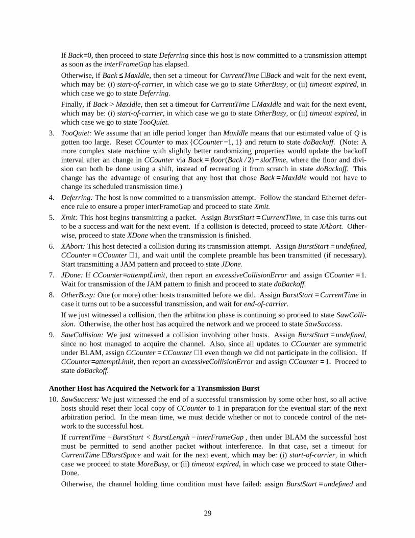
If Back=0, then proceed to state Deferring since this host is now committed to a transmission attemptas soon as the interFrameGap has elapsed.

Otherwise, if Back ≤ MaxIdle, then set a timeout for CurrentTime + Back and wait for the next event,which may be: (i) start-of-carrier, in which case we go to state OtherBusy, or (ii) timeout expired, inwhich case we go to state Deferring.

Finally, if Back > MaxIdle, then set a timeout for CurrentTime + MaxIdle and wait for the next event,which may be: (i) start-of-carrier, in which case we go to state OtherBusy, or (ii) timeout expired, inwhich case we go to state TooQuiet.

3. TooQuiet: We assume that an idle period longer than MaxIdle means that our estimated value of Q isgotten too large. Reset CCounter to max {CCounter −1, 1} and return to state doBackoff. (Note: Amore complex state machine with slightly better randomizing properties would update the backoffinterval after an change in CCounter via Back = floor(Back / 2) − slotTime, where the floor and divi-sion can both be done using a shift, instead of recreating it from scratch in state doBackoff. Thischange has the advantage of ensuring that any host that chose Back = MaxIdle would not have tochange its scheduled transmission time.)

4. Deferring: The host is now committed to a transmission attempt. Follow the standard Ethernet defer-ence rule to ensure a proper interFrameGap and proceed to state Xmit.

5. Xmit: This host begins transmitting a packet. Assign BurstStart = CurrentTime, in case this turns outto be a success and wait for the next event. If a collision is detected, proceed to state XAbort. Other-wise, proceed to state XDone when the transmission is finished.

6. XAbort: This host detected a collision during its transmission attempt. Assign BurstStart = undefined,CCounter = CCounter + 1, and wait until the complete preamble has been transmitted (if necessary).Start transmitting a JAM pattern and proceed to state JDone.

7. JDone: If CCounter=attemptLimit, then report an excessiveCollisionError and assign CCounter = 1.Wait for transmission of the JAM pattern to finish and proceed to state doBackoff.

8. OtherBusy: One (or more) other hosts transmitted before we did. Assign BurstStart = CurrentTime incase it turns out to be a successful transmission, and wait for end-of-carrier.

If we just witnessed a collision, then the arbitration phase is continuing so proceed to state SawColli-sion. Otherwise, the other host has acquired the network and we proceed to state SawSuccess.

9. SawCollision: We just witnessed a collision involving other hosts. Assign BurstStart = undefined,since no host managed to acquire the channel. Also, since all updates to CCounter are symmetricunder BLAM, assign CCounter = CCounter + 1 even though we did not participate in the collision. IfCCounter=attemptLimit, then report an excessiveCollisionError and assign CCounter = 1. Proceed tostate doBackoff.

Another Host has Acquired the Network for a Transmission Burst

10. SawSuccess: We just witnessed the end of a successful transmission by some other host, so all activehosts should reset their local copy of CCounter to 1 in preparation for the eventual start of the nextarbitration period. In the mean time, we must decide whether or not to concede control of the net-work to the successful host.

If currentTime − BurstStart < BurstLength − interFrameGap , then under BLAM the successful hostmust be permitted to send another packet without interference. In that case, set a timeout forCurrentTime + BurstSpace and wait for the next event, which may be: (i) start-of-carrier, in whichcase we proceed to state MoreBusy, or (ii) timeout expired, in which case we proceed to state Other-Done.

Otherwise, the channel holding time condition must have failed: assign BurstStart = undefined and

29

proceed to state doBackoff.

11. OtherDone: The successful host ran out of packets before its channel holding timer expired. AssignBurstStart = undefined and proceed to state doBackoff.

12. MoreBusy: The successful host is continuing to send packets in a burst. Wait until end-of-carrier.

If we just witnessed another successful transmission (the normal case), then proceed to state SawSuc-cess. Otherwise, we witnessed a collision, so we proceed to state SawCollision. (Collision arecaused by hosts that are either newly active, and do not know the state of the algorithm, or are usingthe standard Ethernet algorithm, and do not obey BLAM.)

This Host has Acquired the Network for a Transmission Burst

13. XDone: This host has completed a successful packet transmission. Thus, it is entitled to continue itscurrent burst until its burst length timer runs out, if it can begin transmitting another packet before theother hosts time out and enter state OtherDone. More precisely, if: (i) this host cannot begin its nextpacket transmission before the channel holding timer expires, i.e., currentTime − BurstStart ≥BurstLength − max{interFrameGap, Host Reset Time}, or (ii) the interpacket spacing will be toolarge to prevent the other hosts from triggering its inactivity timer, i.e., BurstSpace − Host Reset Time≤ interFrameGap / 2, or (iii) the host’s transmit queue is empty, then its transmission burst is over:assign BurstStart = undefined and proceed to state Start. Otherwise, this host can continue itstransmission burst: wait for the host interface to be reset (if necessary) and proceed to state XMore, ifstart-of-carrier is not detected in the mean time, or to state XRobbed, otherwise.

14. XMore: This host expects to transmit another packet without interference from anyone else (exceptfor newly active hosts, and those using the standard Ethernet algorithm). Follow the standard Ether-net deference rule to ensure a proper interFrameGap, then start transmitting the next packet, and waitfor the next event. If a collision is detected, proceed to state XAbort. Otherwise, proceed to stateXDone when the transmission is finished.

15. XRobbed: This host had its transmission burst cut short by a collision. Assign BurstStart = undefined,and proceed to state Start.

IV. Performance Comparison

IV.a. Logarithmic versus Linear Reaction Time

Recall that in Section II.a, we showed that BEB is a linear search algorithm, in terms of both therate at which the estimated value of Q increases (Figure 6) and also the average reaction time to a tran-sient overload from the ‘‘Big Bang’’ to the first successful packet (Figure 7). We now show that BLAMhas a fundamental advantage over BEB in terms of its time complexity under these operating conditions.

First, BLAM is essentially a linear search for the logarithm of Q (i.e, a logarithmic search for Q).To see this, consider what happens when the first collision is encountered following the most recentupdate to the collision counter. In this case, all hosts: (i) cancel the remainder of their current backoffdelay (if any); (ii) increment their collision counter (thereby doubling the backoff interval, if CCounterwas below 10); and (iii) initiate a new backoff delay uniformly distributed over the new backoff interval— whether or not they participated in that collision. Thus, like BEB we search for Q using exponentiallyincreasing increments. However, unlike BEB, the ‘cost’ per search step is always one backoff slot timerather than an exponentially increasing number of backoff slot times.

Second, the average time from the ‘‘Big Bang’’ until the first successful packet transmission isalso proportional to the logarithm of Q. Indeed, this O(log2Q) time complexity means that BLAM is fastenough to allow us the luxury of globally resetting the collision counters after a successful packet

30

transmission to improve fairness. To establish this result, we must find the average number of algo-rithmic ‘steps’ (i.e., time, in units of a backoff slot time) from the moment that one successful packettransmission triggers all active hosts to reset their collision counter until the start of the next packettransmission. We do this by solving a system of equations defining the average running time of the algo-rithm as a function of Q. Following the notation from section II.a., we define Lm(C, I) as the averagenumber of backoff slots from now until the first successful transmission occurs in an m-host system, giventhat all active hosts currently have a collision counter value of C, 1 ≤ C <16, and there have been I con-secutive idle slots since the last update to the collision counter, 0 ≤ I < 2. (Since BLAM initializes allhosts to the state C = 1, I = 0 after each successful packet transmission, it follows that Lm(1, 0) representsthe collision resolution time for BLAM, which is comparable to Eq. (5) for BEB.)

Given the above description of how BLAM operates, it is easy to set up a system of equationsfrom which we can determine {Lm(C, I)}. Indeed, all we need to determine is the next state (if any) fol-lowing the three possible channel events (i.e., idle, success, collision) starting from an arbitrary state(C, I). If an idle occurs, then we either move to state (C, I +1) if I +1 < 2 (since we are still below thelimit to the number of consecutive idle slots) or to state (max{C −1, 1}, 0) otherwise. If a success occurs,then we are done at the end of this time step. And, finally, if a collision occurs, then we move to state(C +1, 0) unless C +1 = 16, in which case we report an excessiveCollisionError and return to state (1,0).Thus, it should be clear that {Lm(C, I)} can be found as the solution to following system of equations:

Lm(C, 0) = β(0, m, 1/B).[1 + Lm(C, 1)] + β(1, m, 1/B).1

+ (1 − β(0, m, 1/B) − β(1, m, 1/B)).[1 + Lm(C +1, 0)]

Lm(C, 1) = β(0, m, 1/(B −1)).[1 + Lm(max{C −1, 1}, 0)] + β(1, m, 1/(B −1)).1

+ (1 − β(0, m, 1/(B −1)) − β(1, m, 1/(B −1))).[1 + Lm(C +1, 0)] C < 15 (6)

Lm(15, 1) = β(0, m, 1/(B −1)).[1 + Lm(15, 0)] + β(1, m, 1/(B −1)).1

+ (1 − β(0, m, 1/(B −1)) − β(1, m, 1/(B −1))).[1 + Lm(1, 0)] C = 15

where B = 2min{10, C} is the length of the current backoff interval.

Notice that the above system of equations contains a cyclic dependency: Lm(C, .) depends onLm(C +1, 0) for all C < 15, and Lm(15, .) depends on Lm(1, 0). Thus, Eq. (6) must be solved either itera-tively, or by Gaussian elimination. From this solution, we obtain the conflict resolution time underBLAM, namely Lm(1, 0), which is shown as the dotted curve in Figure 7. The O(log m) time complexityof BLAM is obvious from the Figure, from which we can determine empirically thatLm(1, 0) ∼∼ log2(m) + 1. This is a dramatic improvement over the O(m) time complexity of BEB, espe-cially for large m.

IV.b. No Loss in Throughput, Much Lower and More Predictable Delay

In Figure 11, we have taken our validated simulation model of the experimental setup in [6] andchanged the backoff algorithm in each host to Binary Logarithmic Arbitration. The data in this Figure aredirectly comparable to Figure 3, since we assume that the hosts are fast enough to generate back-to-backpackets (i.e., the time to reset the network interface in each host is assumed to be 0 µsec.). Notice that thecapacity of BLAM is essentially the same as BEB. However, all the standard deviation measures havebeen reduced significantly.

In Figure 12 and Table 3, we show sender-locality and run length information, respectively, forthe same collection of systems as were shown in Figure 4 and Table 2 except for the replacement of BEBby BLAM. It is evident from a comparison of Figures 4 and 12 that BLAM has dramatically increasedthe fairness of the system. Indeed, for all packet lengths greater than 1500 bytes (the holding time limit

31

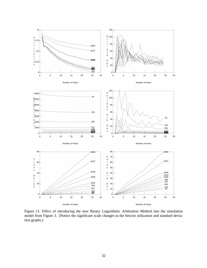
9

9.25

9.5

9.75

10

0 5 10 15 20 25 29

Number of Hosts

Utilization

64128

256512768

1024

1536

2048

3072

4000

0

20

40

60

80

100

120

0 5 10 15 20 25 29

Number of Hosts

Util

Std

Dev

0

2000

4000

6000

8000

10000

12000

14000

0 5 10 15 20 25 29

Number of Hosts

Packets/Sec

64

128

256

51276810241536204830724000 0

20

40

60

80

100

120

0 5 10 15 20 25 29

Number of Hosts

Pkt/Sec

Std

Dev

64

128

25651276810241536204830724000

0

20

40

60

80

0 5 10 15 20 25 29

Number of Hosts

Trans

Delay

64128256512768

1024

1536

2048

3072

4000

0

10

20

30

40

50

60

70

80

0 5 10 15 20 25 29

Number of Hosts

Delay

Std

Dev 64

128256512768

10241536

2048

3072

4000

Figure 11: Effect of introducing the new Binary Logarithmic Arbitration Method into the simulationmodel from Figure 3. (Notice the significant scale changes in the bitwise utilization and standard devia-tion graphs.)

32

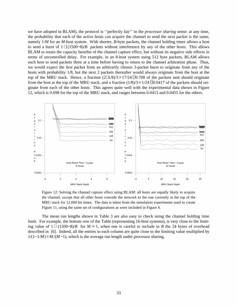
we have adopted in BLAM), the protocol is ‘‘perfectly fair’’ in the processor sharing sense: at any time,the probability that each of the active hosts can acquire the channel to send the next packet is the same,namely 1/M for an M-host system. With shorter, B-byte packets, the channel holding timer allows a hostto send a burst of 1 + © (1500−8)/Bª packets without interference by any of the other hosts. This allowsBLAM to retain the capacity benefits of the channel capture effect, but without its negative side effects interms of uncontrolled delay. For example, in an 8-host system using 512 byte packets, BLAM allowseach host to send packets three at a time before having to return to the channel arbitration phase. Thus,we would expect the first packet from an arbitrarily chosen 3-packet burst to originate from any of thehosts with probability 1/8, but the next 2 packets thereafter would always originate from the host at thetop of the MRU stack. Hence, a fraction (2+1/8)/3 = 17/24 ∼∼ 0.708 of the packets sent should originatefrom the host at the top of the MRU stack, and a fraction (1/8)/3 = 1/24 ∼∼ 0.0417 of the packets should ori-ginate from each of the other hosts. This agrees quite well with the experimental data shown in Figure12, which is 0.698 for the top of the MRU stack, and ranges between 0.0413 and 0.0455 for the others.

-0 2 4 6 8

0.0001

0.001

0.01

0.1

MRU Stack Depth

Acquisition

Prob


64

128

256

5127681024

1536204830724000

-0 5 10 15 20 25

0.0001

0.001

0.01

0.1

MRU Stack Depth

Acquisition

Prob


64

128

256

51276241024

15362042430724000

Figure 12: Solving the channel capture effect using BLAM: all hosts are equally likely to acquirethe channel, except that all other hosts concede the network to the one currently at the top of theMRU stack for 12,000 bit times. The data is taken from the simulation experiments used to createFigure 11, using the same set of configurations as were included in Figure 4.

The mean run lengths shown in Table 3 are also easy to check using the channel holding timelimit. For example, the bottom row of the Table (representing 16-host systems), is very close to the limit-ing value of 1 + « (1500−8)/B¬ for M >> 1, when one is careful to include in B the 24 bytes of overheaddescribed in [6]. Indeed, all the entries in each column are quite close to the limiting value multiplied by1/(1−1/M) = M /(M −1), which is the average run length under processor sharing.

33

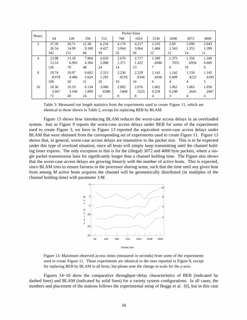
��Packet Sizes® ®�®�®�®�®�®�®�®�®�®�®�®�®�®�®�®�®�®�®�®�®�®�®�®�®�®�®�®�®�®�®�®�®�®�®�®�®�®�®�®�®�®�®�®�®�®�®�®�®�®�®�®�®�®�®�®�®�®�®�®�®�®�®�®�®�®�®�®�®�®�®�®�®�®�®�®�®�®�®�®�®�®�®�®�®�®�®�®�®�®�®�®�®Hosts:

64 128 256 512 768 1024 1536 2048 3072 4000¯ ¯�¯�¯�¯�¯�¯�¯�¯�¯�¯�¯�¯�¯�¯�¯�¯�¯�¯�¯�¯�¯�¯�¯�¯�¯�¯�¯�¯�¯�¯�¯�¯�¯�¯�¯�¯�¯�¯�¯�¯�¯�¯�¯�¯�¯�¯�¯�¯�¯�¯�¯�¯�¯�¯�¯�¯�¯�¯�¯�¯�¯�¯�¯�¯�¯�¯�¯�¯�¯�¯�¯�¯�¯�¯�¯�¯�¯�¯�¯�¯�¯�¯�¯�¯�¯�¯�¯�¯�¯�¯�¯�¯�¯�¯�¯�¯�¯�¯�¯�¯�¯¯ ¯�¯�¯�¯�¯�¯�¯�¯�¯�¯�¯�¯�¯�¯�¯�¯�¯�¯�¯�¯�¯�¯�¯�¯�¯�¯�¯�¯�¯�¯�¯�¯�¯�¯�¯�¯�¯�¯�¯�¯�¯�¯�¯�¯�¯�¯�¯�¯�¯�¯�¯�¯�¯�¯�¯�¯�¯�¯�¯�¯�¯�¯�¯�¯�¯�¯�¯�¯�¯�¯�¯�¯�¯�¯�¯�¯�¯�¯�¯�¯�¯�¯�¯�¯�¯�¯�¯�¯�¯�¯�¯�¯�¯�¯�¯�¯�¯�¯�¯�¯�¯2 37.30 20.71 12.38 6.234 4.170 4.217 2.105 2.09 2.090 2.043

26.54 14.99 9.180 4.427 3.064 3.064 1.484 1.543 1.553 1.399342 151 84 39 32 26 12 13 14 11° °�°�°�°�°�°�°�°�°�°�°�°�°�°�°�°�°�°�°�°�°�°�°�°�°�°�°�°�°�°�°�°�°�°�°�°�°�°�°�°�°�°�°�°�°�°�°�°�°�°�°�°�°�°�°�°�°�°�°�°�°�°�°�°�°�°�°�°�°�°�°�°�°�°�°�°�°�°�°�°�°�°�°�°�°�°�°�°�°�°�°�°�°�°�°�°�°�°�°�°�°

4 23.98 13.18 7.964 4.020 2.670 2.717 1.349 1.375 1.356 1.34913.14 6.965 4.304 2.088 1.371 1.425 .6946 .7055 .6956 0.669

126 70 48 24 14 13 7 6 10 6± ±�±�±�±�±�±�±�±�±�±�±�±�±�±�±�±�±�±�±�±�±�±�±�±�±�±�±�±�±�±�±�±�±�±�±�±�±�±�±�±�±�±�±�±�±�±�±�±�±�±�±�±�±�±�±�±�±�±�±�±�±�±�±�±�±�±�±�±�±�±�±�±�±�±�±�±�±�±�±�±�±�±�±�±�±�±�±�±�±�±�±�±�±�±�±�±�±�±�±�±�±8 19.74 10.97 6.602 3.313 2.236 2.229 1.143 1.142 1.150 1.145

8.078 4.486 2.624 1.293 .8218 .8166 .4106 0.408 .4222 .4100108 50 31 18 10 10 6 4 4 5² ²�²�²�²�²�²�²�²�²�²�²�²�²�²�²�²�²�²�²�²�²�²�²�²�²�²�²�²�²�²�²�²�²�²�²�²�²�²�²�²�²�²�²�²�²�²�²�²�²�²�²�²�²�²�²�²�²�²�²�²�²�²�²�²�²�²�²�²�²�²�²�²�²�²�²�²�²�²�²�²�²�²�²�²�²�²�²�²�²�²�²�²�²�²�²�²�²�²�²�²�²

16 18.36 10.19 6.134 3.088 2.082 2.076 1.062 1.061 1.063 1.0565.667 3.166 1.899 .8388 .5468 .5525 0.258 0.248 .2641 .2467

72 40 24 12 8 8 4 3 4 4³ ³�³�³�³�³�³�³�³�³�³�³�³�³�³�³�³�³�³�³�³�³�³�³�³�³�³�³�³�³�³�³�³�³�³�³�³�³�³�³�³�³�³�³�³�³�³�³�³�³�³�³�³�³�³�³�³�³�³�³�³�³�³�³�³�³�³�³�³�³�³�³�³�³�³�³�³�³�³�³�³�³�³�³�³�³�³�³�³�³�³�³�³�³�³�³�³�³�³�³�³�³´´´´´´´´´´´´´´´´´´´

´´´´´´´´´´´´´´´´´´´

´´´´´´´´´´´´´´´´´´´

´´´´´´´´´´´´´´´´´´

´´´´´´´´´´´´´´´´´´

´´´´´´´´´´´´´´´´´´

´´´´´´´´´´´´´´´´´´

´´´´´´´´´´´´´´´´´´

´´´´´´´´´´´´´´´´´´

´´´´´´´´´´´´´´´´´´

´´´´´´´´´´´´´´´´´´

´´´´´´´´´´´´´´´´´´

´´´´´´´´´´´´´´´´´´´

Table 3: Measured run length statistics from the experiments used to create Figure 11, which areidentical to those shown in Table 2, except for replacing BEB by BLAM.

Figure 13 shows how introducing BLAM reduces the worst-case access delays in an overloadedsystem. Just as Figure 9 reports the worst-case access delays under BEB for some of the experimentsused to create Figure 3, we have in Figure 13 reported the equivalent worst-case access delays underBLAM that were obtained from the corresponding set of experiments used to create Figure 11. Figure 13shows that, in general, worst-case access delays are insensitive to the packet size. This is to be expectedunder this type of overload situation, since all hosts will simply keep transmitting until the channel hold-ing timer expires. The only exception to this is for the (illegal) 3072 and 4000 byte packets, where a sin-gle packet transmission lasts for significantly longer than a channel holding time. The Figure also showsthat the worst-case access delays are growing linearly with the number of active hosts. This is expected,since BLAM tries to ensure fairness in the processor sharing sense, such that the time until any given hostfrom among M active hosts acquires the channel will be geometrically distributed (in multiples of thechannel holding time) with parameter 1/M.

.01

.02

.05

.1

.2

.5

64 128 256 512 1024 2048 4000

Packet Size

Max

Delay

2

4

8

16

Figure 13: Maximum observed access times (measured in seconds) from some of the experimentsused to create Figure 11. These experiments are identical to the ones reported in Figure 9, exceptfor replacing BEB by BLAM in all hosts, but please note the change in scale for the y-axis.

Figures 14−16 show the comparative throughput−delay characteristics of BEB (indicated bydashed lines) and BLAM (indicated by solid lines) for a variety system configurations. In all cases, thenumbers and placement of the stations follows the experimental setup of Boggs et al. [6], but in this case

34

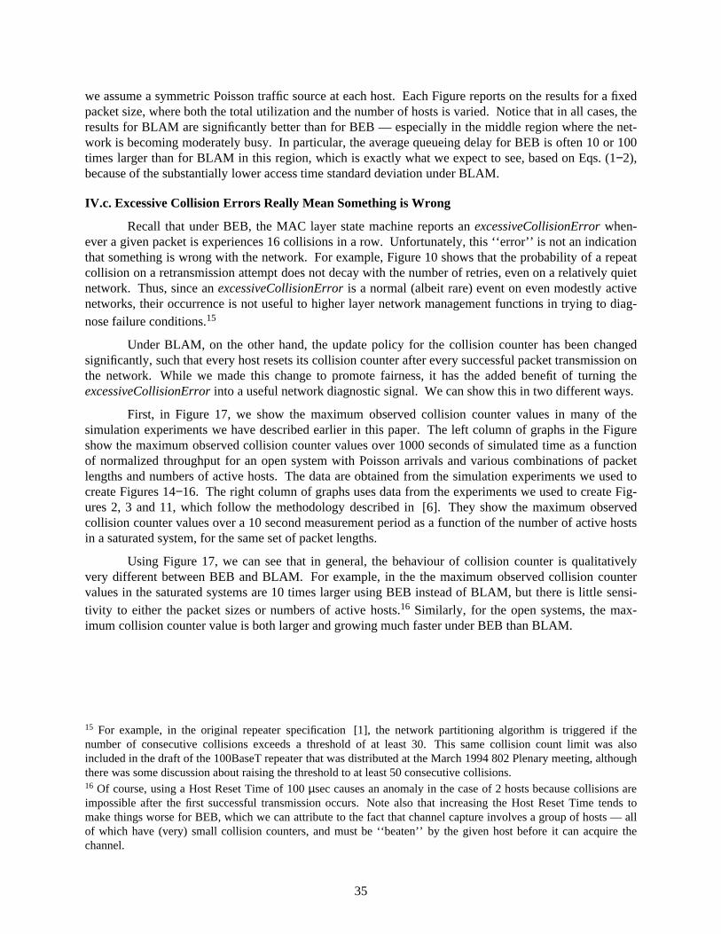
we assume a symmetric Poisson traffic source at each host. Each Figure reports on the results for a fixedpacket size, where both the total utilization and the number of hosts is varied. Notice that in all cases, theresults for BLAM are significantly better than for BEB — especially in the middle region where the net-work is becoming moderately busy. In particular, the average queueing delay for BEB is often 10 or 100times larger than for BLAM in this region, which is exactly what we expect to see, based on Eqs. (1−2),because of the substantially lower access time standard deviation under BLAM.

IV.c. Excessive Collision Errors Really Mean Something is Wrong

Recall that under BEB, the MAC layer state machine reports an excessiveCollisionError when-ever a given packet is experiences 16 collisions in a row. Unfortunately, this ‘‘error’’ is not an indicationthat something is wrong with the network. For example, Figure 10 shows that the probability of a repeatcollision on a retransmission attempt does not decay with the number of retries, even on a relatively quietnetwork. Thus, since an excessiveCollisionError is a normal (albeit rare) event on even modestly activenetworks, their occurrence is not useful to higher layer network management functions in trying to diag-nose failure conditions.15

Under BLAM, on the other hand, the update policy for the collision counter has been changedsignificantly, such that every host resets its collision counter after every successful packet transmission onthe network. While we made this change to promote fairness, it has the added benefit of turning theexcessiveCollisionError into a useful network diagnostic signal. We can show this in two different ways.

First, in Figure 17, we show the maximum observed collision counter values in many of thesimulation experiments we have described earlier in this paper. The left column of graphs in the Figureshow the maximum observed collision counter values over 1000 seconds of simulated time as a functionof normalized throughput for an open system with Poisson arrivals and various combinations of packetlengths and numbers of active hosts. The data are obtained from the simulation experiments we used tocreate Figures 14−16. The right column of graphs uses data from the experiments we used to create Fig-ures 2, 3 and 11, which follow the methodology described in [6]. They show the maximum observedcollision counter values over a 10 second measurement period as a function of the number of active hostsin a saturated system, for the same set of packet lengths.

Using Figure 17, we can see that in general, the behaviour of collision counter is qualitativelyvery different between BEB and BLAM. For example, in the the maximum observed collision countervalues in the saturated systems are 10 times larger using BEB instead of BLAM, but there is little sensi-tivity to either the packet sizes or numbers of active hosts.16 Similarly, for the open systems, the max-imum collision counter value is both larger and growing much faster under BEB than BLAM.

µ µ�µ�µ�µ�µ�µ�µ�µ�µ�µ�µ�µ�µ�µ15 For example, in the original repeater specification [1], the network partitioning algorithm is triggered if thenumber of consecutive collisions exceeds a threshold of at least 30. This same collision count limit was alsoincluded in the draft of the 100BaseT repeater that was distributed at the March 1994 802 Plenary meeting, althoughthere was some discussion about raising the threshold to at least 50 consecutive collisions.16 Of course, using a Host Reset Time of 100 µsec causes an anomaly in the case of 2 hosts because collisions areimpossible after the first successful transmission occurs. Note also that increasing the Host Reset Time tends tomake things worse for BEB, which we can attribute to the fact that channel capture involves a group of hosts — allof which have (very) small collision counters, and must be ‘‘beaten’’ by the given host before it can acquire thechannel.

35

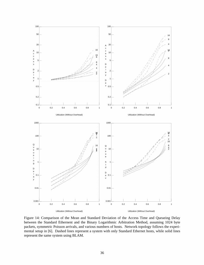
0.1

0.2

0.5

1

2

5

10

20

50

100

0 0.2 0.4 0.6 0.8 1

Utilization (Without Overhead)

Access

Delay . . . . . . . . . . . . . . . . . . . . . . . . . . . . . . . . . . . . . . . . . . . . . . . . . ..

.

.

.

.

.

.

.

.

.

.

.

.

.

.

.

.

.

.

.

.

.

.

.

.

.

.

.

.

.

.

.

.

.

.

.

.

.

.

.

.

.

.

.

.

.

2

4

8

16

2

4

8

16

0.1

0.2

0.5

1

2

5

10

20

50

100

0 0.2 0.4 0.6 0.8 1


Access

Delay

Dev

.

.

.

.

.

.

.

.

.

.

.

.

.

.

.

.

.

.

.

.

.

.

.

.

.

.

.

.

.

.

.

.

.

.

.

.

.

.

.

.

.

.

.

.

.

.

.

.

.

.

.

.

.

.

.

.

.

.

.

.

.

.

.

.

.

.

2

4

8

16

2

4

8

16

0.001

0.01

0.1

1

10

100

1000

0 0.2 0.4 0.6 0.8 1


Queueing

Delay

.

.

.

.

.

.

.

.

.

.

.

.

.

.

.

.

.

.

.

.

.

.

.

.

.

.

.

.

.

.

.

.

.

.

.

.

.

.

.

.

.

.

.

.

.

.

.

.

.

.

.

.

.

.

.

.

.

.

.

.

.

.

.

.

.

.

24816

248

16

0.001

0.01

0.1

1

10

100

1000

0 0.2 0.4 0.6 0.8 1


Queue

Std

Dev

.

.

.

.

.

.

.

.

.

.

.

.

.

.

.

.

.

.

.

.

.

.

.

.

.

.

.

.

.

.

.

.

.

.

.

.

.

.

.

.

.

.

.

.

.

.

.

.

.

.

.

.

.

.

.

.

.

.

.

.

.

.

.

.

.

.

2

4816

248

16

Figure 14: Comparison of the Mean and Standard Deviation of the Access Time and Queueing Delaybetween the Standard Ethernent and the Binary Logarithmic Arbitration Method, assuming 1024 bytepackets, symmetric Poisson arrivals, and various numbers of hosts. Network topology follows the experi-mental setup in [6]. Dashed lines represent a system with only Standard Ethernet hosts, while solid linesrepresent the same system using BLAM.

36

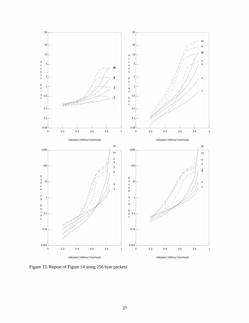
0.05

0.1

0.2

0.5

1

2

5

10

20

50

0 0.2 0.4 0.6 0.8 1


Access

Delay

. . . . . . . . . . . . . . . . . . . . . . . . . . . . . . . . . . . . . . . . . . . . . . .....................................................

2

4

8

16

2

4

8

16

0.05

0.1

0.2

0.5

1

2

5

10

20

50

0 0.2 0.4 0.6 0.8 1


Access

Delay

Dev

.

.

.

.

.

.

.

.

.

.

.

.

.

.

.

.

.

.

.

.

.

.

.

.

.

.

.

.

.

.

.

.

.

.

.

.

.

.

.

.

.

.

.

.

.

.

.

.

.

.

.

.

.

.

.

.

.

.

.

.

.

.

.

.

.

.

2

4

8

16

2

4

8

16

0.001

0.01

0.1

1

10

100

1000

0 0.2 0.4 0.6 0.8 1


Queueing

Delay

.

.

.

.

.

.

.

.

.

.

.

.

.

.

.

.

.

.

.

.

.

.

.

.

.

.

.

.

.

.

.

.

.

.

.

.

.

.

.

.

.

.

.

.

.

.

.

.

.

.

.

.

.

.

.

.

.

.

.

.

.

.

.

.

.

.

2

48

16

2

4

8

16

0.001

0.01

0.1

1

10

100

1000

0 0.2 0.4 0.6 0.8 1


Queue

Std

Dev

.

.

.

.

.

.

.

.

.

.

.

.

.

.

.

.

.

.

.

.

.

.

.

.

.

.

.

.

.

.

.

.

.

.

.

.

.

.

.

.

.

.

.

.

.

.

.

.

.

.

.

.

.

.

.

.

.

.

.

.

.

.

.

.

.

.

2

4

8

16

2

4

8

16

Figure 15: Repeat of Figure 14 using 256 byte packets.

37

0.02

0.05

0.1

0.2

0.5

1

2

5

10

20

0 0.2 0.4 0.6 0.8 1


Access

Delay

. . . . . . . . . . . . . . . . . . . . . . . . . . . . . . . . . . . . . . .........................................................

2

4

8

16

2

4

8

16

0.02

0.05

0.1

0.2

0.5

1

2

5

10

20

0 0.2 0.4 0.6 0.8 1


Access

Delay

Dev

.

.

.

.

.

.

.

.

.

.

.

.

.

.

.

.

.

.

.

.

.

.

.

.

.

.

.

.

.

.

.

.

.

.

.

.

.

.

.

.

.

.

.

.

.

.

.

.

.

.

.

.

.

.

.

.

.

.

.

.

.

.

.

.

.

.

2

4

8

16

2

4

8

16

0.001

0.01

0.1

1

10

100

1000

0 0.2 0.4 0.6 0.8 1


Queueing

Delay

.

.

.

.

.

.

.

.

.

.

.

.

.

.

.

.

.

.

.

.

.

.

.

.

.

.

.

.

.

.

.

.

.

.

.

.

.

.

.

.

.

.

.

.

.

.

.

.

.

.

.

.

.

.

.

.

.

.

.

.

.

.

.

.

.

.

2

48

16

2

4

8

16

0.001

0.01

0.1

1

10

100

1000

0 0.2 0.4 0.6 0.8 1


Queue

Std

Dev

.

.

.

.

.

.

.

.

.

.

.

.

.

.

.

.

.

.

.

.

.

.

.

.

.

.

.

.

.

.

.

.

.

.

.

.

.

.

.

.

.

.

.

.

.

.

.

.

.

.

.

.

.

.

.

.

.

.

.

.

.

.

.

.

.

.

2

48

16

2

4

8

16

Figure 16: Repeat of Figure 14 using 64 byte packets.

38

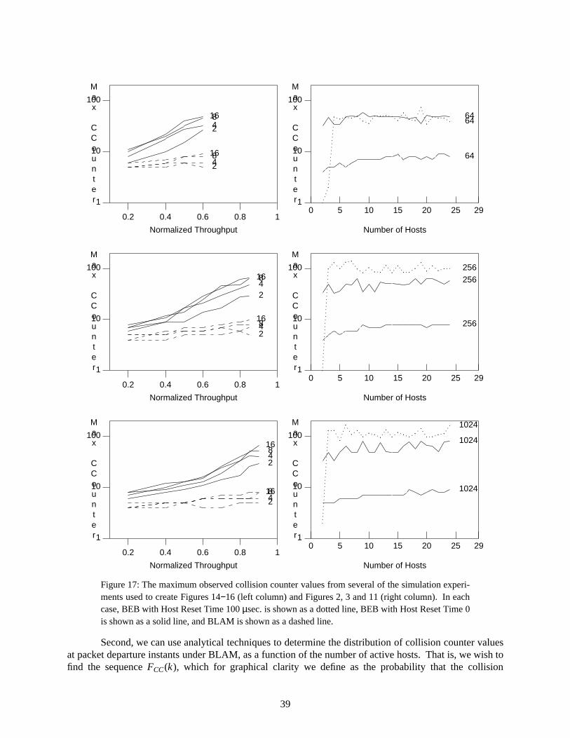
1

10

100

0 5 10 15 20 25 29

Number of Hosts

Max

CCounter .

............................ . .. . .. . .. . .. . .. . .. .

. .. . .. . .. . .. . .. .. .. . . .. . ..

........... .

. .. . .. . .. . . 6464

64

0.2 0.4 0.6 0.8 1

1

10

100

Normalized Throughput

Max

CCounter

24816

24816

1

10

100

0 5 10 15 20 25 29

Number of Hosts

Max

CCounter .

.

.

.

.

.

.

.

.

.

.

.

.

.

.

.

.

.

.

.

.

.

.

.

.

.

.

.

.

.

.. .. .. . .. .

. .. . .. . . .. . .. . .. . .. . .. .. .. . . .. .

. .. . . .. . .. . .. . .. . . .. . .. . .. . .. . . 256256

256

0.2 0.4 0.6 0.8 1

1

10

100


Max

CCounter

24816

24816

1

10

100

0 5 10 15 20 25 29

Number of Hosts

Max

CCounter

.

.

.

.

.

.

.

.

.

.

.

.

.

.

.

.

.

.

.

.

.

.

.

.

.

.

.

.

.. . ............ . .

.. . .. . . .. . .. . .. . .. .. .. . . .. . .. . .. . .. . .. . .. . . .. . .. . .. . .. .

. . 1024

1024

1024

0.2 0.4 0.6 0.8 1

1

10

100


Max

CCounter

24816

24816

Figure 17: The maximum observed collision counter values from several of the simulation experi-ments used to create Figures 14−16 (left column) and Figures 2, 3 and 11 (right column). In eachcase, BEB with Host Reset Time 100 µsec. is shown as a dotted line, BEB with Host Reset Time 0is shown as a solid line, and BLAM is shown as a dashed line.

Second, we can use analytical techniques to determine the distribution of collision counter valuesat packet departure instants under BLAM, as a function of the number of active hosts. That is, we wish tofind the sequence FCC(k), which for graphical clarity we define as the probability that the collision

39

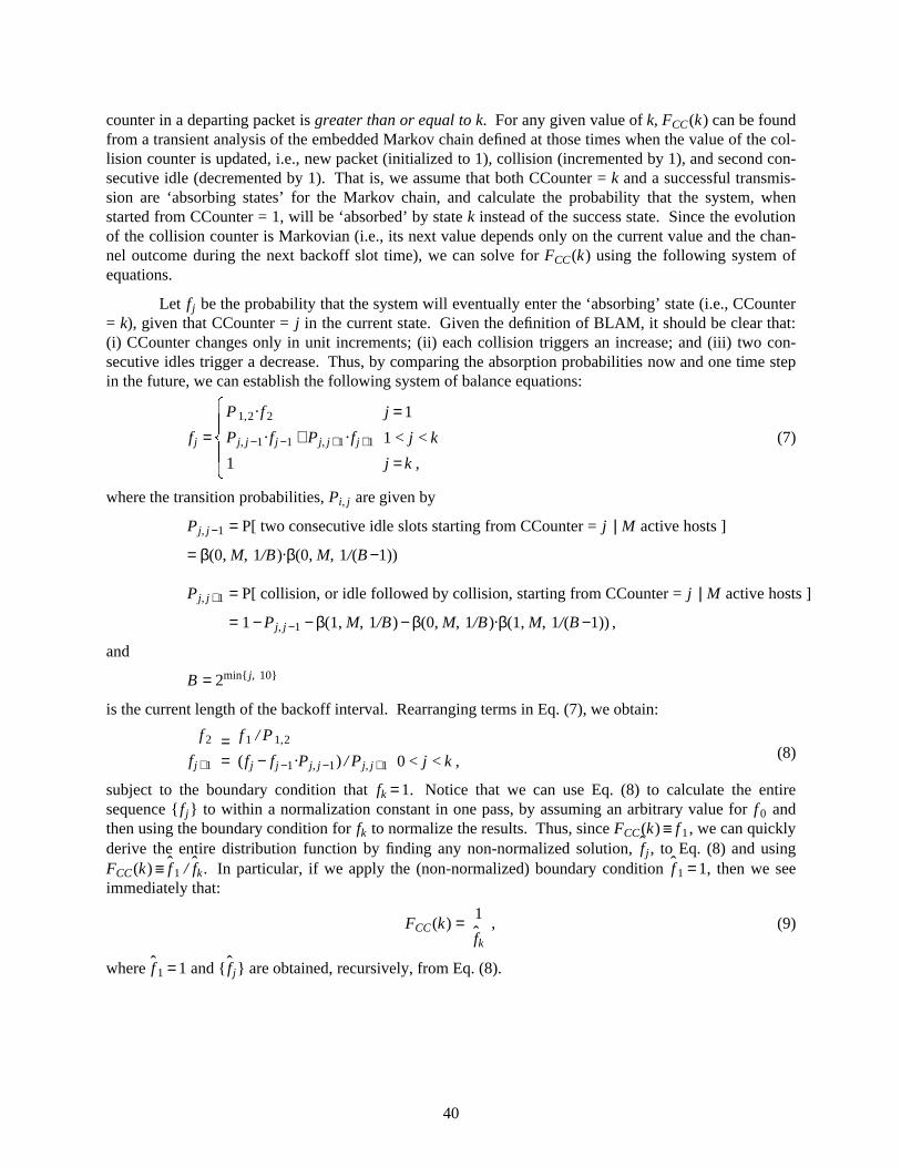
counter in a departing packet is greater than or equal to k. For any given value of k, FCC(k) can be foundfrom a transient analysis of the embedded Markov chain defined at those times when the value of the col-lision counter is updated, i.e., new packet (initialized to 1), collision (incremented by 1), and second con-secutive idle (decremented by 1). That is, we assume that both CCounter = k and a successful transmis-sion are ‘absorbing states’ for the Markov chain, and calculate the probability that the system, whenstarted from CCounter = 1, will be ‘absorbed’ by state k instead of the success state. Since the evolutionof the collision counter is Markovian (i.e., its next value depends only on the current value and the chan-nel outcome during the next backoff slot time), we can solve for FCC(k) using the following system ofequations.

Let f j be the probability that the system will eventually enter the ‘absorbing’ state (i.e., CCounter= k), given that CCounter = j in the current state. Given the definition of BLAM, it should be clear that:(i) CCounter changes only in unit increments; (ii) each collision triggers an increase; and (iii) two con-secutive idles trigger a decrease. Thus, by comparing the absorption probabilities now and one time stepin the future, we can establish the following system of balance equations:

f j =

¶·¸ ·¹ 1

Pj, j −1.f j −1 + Pj, j +1

.f j +1

P 1,2.f 2

j = k ,

1 < j < k

j = 1

(7)

where the transition probabilities, Pi, j are given by

Pj, j −1 = P[ two consecutive idle slots starting from CCounter = j | M active hosts ]

= β(0, M, 1/B).β(0, M, 1/(B −1))

Pj, j +1 = P[ collision, or idle followed by collision, starting from CCounter = j | M active hosts ]

= 1 − Pj, j −1 − β(1, M, 1/B) − β(0, M, 1/B).β(1, M, 1/(B −1)) ,

and

B = 2min{ j, 10}

is the current length of the backoff interval. Rearranging terms in Eq. (7), we obtain:

f j +1

f 2

==

(f j − f j −1.Pj, j −1) / Pj, j +1

f 1 / P 1,2

0 < j < k , (8)

subject to the boundary condition that fk = 1. Notice that we can use Eq. (8) to calculate the entiresequence {f j} to within a normalization constant in one pass, by assuming an arbitrary value for f 0 andthen using the boundary condition for fk to normalize the results. Thus, since FCC(k) ≡ f 1 , we can quicklyderive the entire distribution function by finding any non-normalized solution, f̂ j , to Eq. (8) and usingFCC(k) ≡ f̂ 1 / f̂k. In particular, if we apply the (non-normalized) boundary condition f̂ 1 = 1, then we seeimmediately that:

FCC(k) =f̂k

1º º�º , (9)

where f̂ 1 = 1 and { f̂ j} are obtained, recursively, from Eq. (8).

40

-0 5 10 15 20

1

10−2

10−4

10−6

10−8

10−10

10−12

10−14

Maximum Collision Counter

Probability

+ +. . . . . .

+. . . . . .

+

. . . . . . . .

+

..........

+

............

+

......

........

+

..................

+ +. . . . . .+

. . . . . .

+. . . . . .

+

. . . . . . . .

+

. . . . . . . . .

+

.....

.....

.

+

.............

+

....................

+ +. . . . . . +. . . . . .+

. . . . . .

+. . . . . .

+

. . . . . . . .

+

. . . . . . . . .

+

...........

+

.............

+

.....................

+ +. . . . . . +. . . . . . +. . . . . .+

. . . . . .

+. . . . . .

+

. . . . . . .

+

. . . . . . . . .

+

...........

+

.....

.......

.

+

.....................

+ +. . . . . . +. . . . . +. . . . . . +. . . . . .+

. . . . . .

+. . . . . .

+

. . . . . . .

+

. . . . . . . . .

+

...........

+

.....

........

+

.......

...............

+ +. . . . . . +. . . . . +. . . . . . +. . . . . . +. . . . . .+

. . . . . .

+. . . . . .

+

. . . . . . .

+

. . . . . . . . .

+

...........

+

...........

+

...........

+

...............

+ +. . . . . . +. . . . . +. . . . . . +. . . . . . +. . . . . . +. . . . . .+

. . . . . .

+. . . . . .

+

. . . . . . .

+

. . . . . . . . .

+

. . . . . . . . .

+

. . . . . . . . .

+

. . . . . . . . .

+

. . . . . . . . .

+

. . . . . . . . .. . . . . .

+ +. . . . . . +. . . . . +. . . . . . +. . . . . . +. . . . . +. . . . . . +. . . . . .+

. . . . . .

+. . . . . .

+

. . . . . . .

+

. . . . . . . .

+

. . . . . . . .

+

. . . . . . . .

+

. . . . . . . .

+

. . . . . . . .

+

. . . . . . . .

+

. . . . . . . .

+

. . . . . . . .

+

. . . . . . . .

+ +. . . . . . +. . . . . +. . . . . . +. . . . . . +. . . . . +. . . . . . +. . . . . . +. . . . . .+

. . . . . .

+. . . . . .

+. . . . . .

+. . . . . .

+. . . . . .

+. . . . . .

+. . . . . .

+. . . . . .

+. . . . . .

+. . . . . .

+. . . . . .

+ +. . . . . . +. . . . . +. . . . . . +. . . . . . +. . . . . +. . . . . . +. . . . . . +. . . . . . +. . . . . .+

. . . . . .+

. . . . . .+

. . . . . .+

. . . . . .+

. . . . . .+

. . . . . .+

. . . . . .+

. . . . . .+

. . . . . .+

. . . . . .

Figure 18: The probability distribution function, FCC(k), for the collision counter of a departingpacket under BLAM, conditioned on M, the number of hosts currently active. (Curves from left toright correspond to M = 2, 4, 8, 16, 32, 64, 128, 256, 512, 1024.)

Figure 18 shows FCC(k) for various numbers of active hosts. It is interesting to note how theshapes of the various curves are affected by the relation between the collision counter and the length ofthe backoff interval. As long as the collision counter is below 10, then successive curves are essentiallythe same except for translation to the right. This is to be expected, since the number of attempts per slotshould be almost identical if we both double the number of active hosts (i.e., move to the next curve) andhalve each of their respective transmission probabilities (i.e., increase CCounter by one). Furthermore,the continuation of each curve beyond CCounter = 10 is just a tangent line, as we would expect since thebackoff interval, B, does not change any more. Thus, we are merely looking at the tail of a geometric dis-tribution, which is a straight line on a semi-log scale. It is also interesting to compare the maximumobserved collision counter values under BLAM from Figure 17 to FCC(k). In particular, we see that thoseobserved maxima correspond quite closely to the collision counter values for which FCC(k) ∼∼ 10−4 .

Notice that for all M ≤ 128, the probability of falsely triggering an excessiveCollisionError isnegligible (i.e., 10−14 or less). In the worst case (namely a saturated 1024 host network), this probabilityincreases to 1/491, which is perhaps too large to be taken seriously as an indication of a real problem withthe network. However, if the performance of the system with hundreds of hosts on the same collisiondomain is an important issue, then we suggest waiting for the collision counter to reach 20 before declar-ing an excessiveCollisionError. This change reduces the worst-case probability of falsely triggering thecondition to 1/23267, which seems more than adequate for signalling a real error condition in the net-work.

IV.d. Coexistence of Old and New

Ethernet-like random-access systems have been studied extensively for more than 20 years, so atthis point it is really not that difficult to find a new algorithm that has better performance. However, it isnot sufficient just to come up with a better algorithm because we cannot simply throw away all existingEthernet-compatible equipment and start fresh — and if we did try it, we might very well end up with a

41

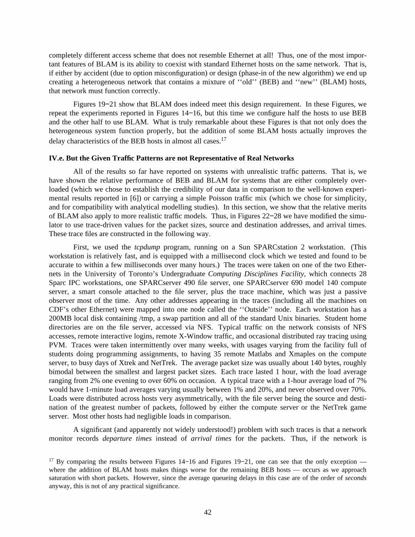
completely different access scheme that does not resemble Ethernet at all! Thus, one of the most impor-tant features of BLAM is its ability to coexist with standard Ethernet hosts on the same network. That is,if either by accident (due to option misconfiguration) or design (phase-in of the new algorithm) we end upcreating a heterogeneous network that contains a mixture of ‘‘old’’ (BEB) and ‘‘new’’ (BLAM) hosts,that network must function correctly.

Figures 19−21 show that BLAM does indeed meet this design requirement. In these Figures, werepeat the experiments reported in Figures 14−16, but this time we configure half the hosts to use BEBand the other half to use BLAM. What is truly remarkable about these Figures is that not only does theheterogeneous system function properly, but the addition of some BLAM hosts actually improves thedelay characteristics of the BEB hosts in almost all cases.17

IV.e. But the Given Traffic Patterns are not Representative of Real Networks

All of the results so far have reported on systems with unrealistic traffic patterns. That is, wehave shown the relative performance of BEB and BLAM for systems that are either completely over-loaded (which we chose to establish the credibility of our data in comparison to the well-known experi-mental results reported in [6]) or carrying a simple Poisson traffic mix (which we chose for simplicity,and for compatibility with analytical modelling studies). In this section, we show that the relative meritsof BLAM also apply to more realistic traffic models. Thus, in Figures 22−28 we have modified the simu-lator to use trace-driven values for the packet sizes, source and destination addresses, and arrival times.These trace files are constructed in the following way.

First, we used the tcpdump program, running on a Sun SPARCstation 2 workstation. (Thisworkstation is relatively fast, and is equipped with a millisecond clock which we tested and found to beaccurate to within a few milliseconds over many hours.) The traces were taken on one of the two Ether-nets in the University of Toronto’s Undergraduate Computing Disciplines Facility, which connects 28Sparc IPC workstations, one SPARCserver 490 file server, one SPARCserver 690 model 140 computeserver, a smart console attached to the file server, plus the trace machine, which was just a passiveobserver most of the time. Any other addresses appearing in the traces (including all the machines onCDF’s other Ethernet) were mapped into one node called the ‘‘Outside’’ node. Each workstation has a200MB local disk containing /tmp, a swap partition and all of the standard Unix binaries. Student homedirectories are on the file server, accessed via NFS. Typical traffic on the network consists of NFSaccesses, remote interactive logins, remote X-Window traffic, and occasional distributed ray tracing usingPVM. Traces were taken intermittently over many weeks, with usages varying from the facility full ofstudents doing programming assignments, to having 35 remote Matlabs and Xmaples on the computeserver, to busy days of Xtrek and NetTrek. The average packet size was usually about 140 bytes, roughlybimodal between the smallest and largest packet sizes. Each trace lasted 1 hour, with the load averageranging from 2% one evening to over 60% on occasion. A typical trace with a 1-hour average load of 7%would have 1-minute load averages varying usually between 1% and 20%, and never observed over 70%.Loads were distributed across hosts very asymmetrically, with the file server being the source and desti-nation of the greatest number of packets, followed by either the compute server or the NetTrek gameserver. Most other hosts had negligible loads in comparison.

A significant (and apparently not widely understood!) problem with such traces is that a networkmonitor records departure times instead of arrival times for the packets. Thus, if the network is

» »�»�»�»�»�»�»�»�»�»�»�»�»�»17 By comparing the results between Figures 14−16 and Figures 19−21, one can see that the only exception —where the addition of BLAM hosts makes things worse for the remaining BEB hosts — occurs as we approachsaturation with short packets. However, since the average queueing delays in this case are of the order of secondsanyway, this is not of any practical significance.

42

0.1

0.2

0.5

1

2

5

10

20

50

100

0 0.2 0.4 0.6 0.8 1


Access

Delay . . . . . . . . . . . . . . . . . . . . . . . . . . . . . . . . . . . . . . . . . . . . . . . . . ..

.

.

.

.

.

.

.

.

.

.

.

.

.

.

.

.

.

.

.

.

.

.

.

.

.

.

.

.

.

.

.

.

.

.

.

.

.

.

.

.

.

.

.

.

.

2

4

8

16

2

4

816

0.1

0.2

0.5

1

2

5

10

20

50

100

0 0.2 0.4 0.6 0.8 1


Access

Delay

Dev

.

.

.

.

.

.

.

.

.

.

.

.

.

.

.

.

.

.

.

.

.

.

.

.

.

.

.

.

.

.

.

.

.

.

.

.

.

.

.

.

.

.

.

.

.

.

2

4

8

16

2

4816

0.001

0.01

0.1

1

10

100

1000

0 0.2 0.4 0.6 0.8 1


Queueing

Delay

.

.

.

.

.

.

.

.

.

.

.

.

.

.

.

.

.

.

.

.

.

.

.

.

.

.

.

.

.

.

.

.

.

.

2

4

816

2

4

8

16

0.001

0.01

0.1

1

10

100

1000

0 0.2 0.4 0.6 0.8 1


Queue

Std

Dev

.

.

.

.

.

.

.

.

.

.

.

.

.

.

.

.

.

.

.

.

.

.

.

.

.

.

.

.

.

.

.

.

.

.

2

4

816

2

4

816

Figure 19: Effects of mixing hosts using the Standard Ethernet algorithm and the Binary LogarithmicArbitration Method on the same network. Same setup as Figure 14, but this time, half the hosts use theStandard Ethernet protocol (dashed lines) and the other half use BLAM.

43

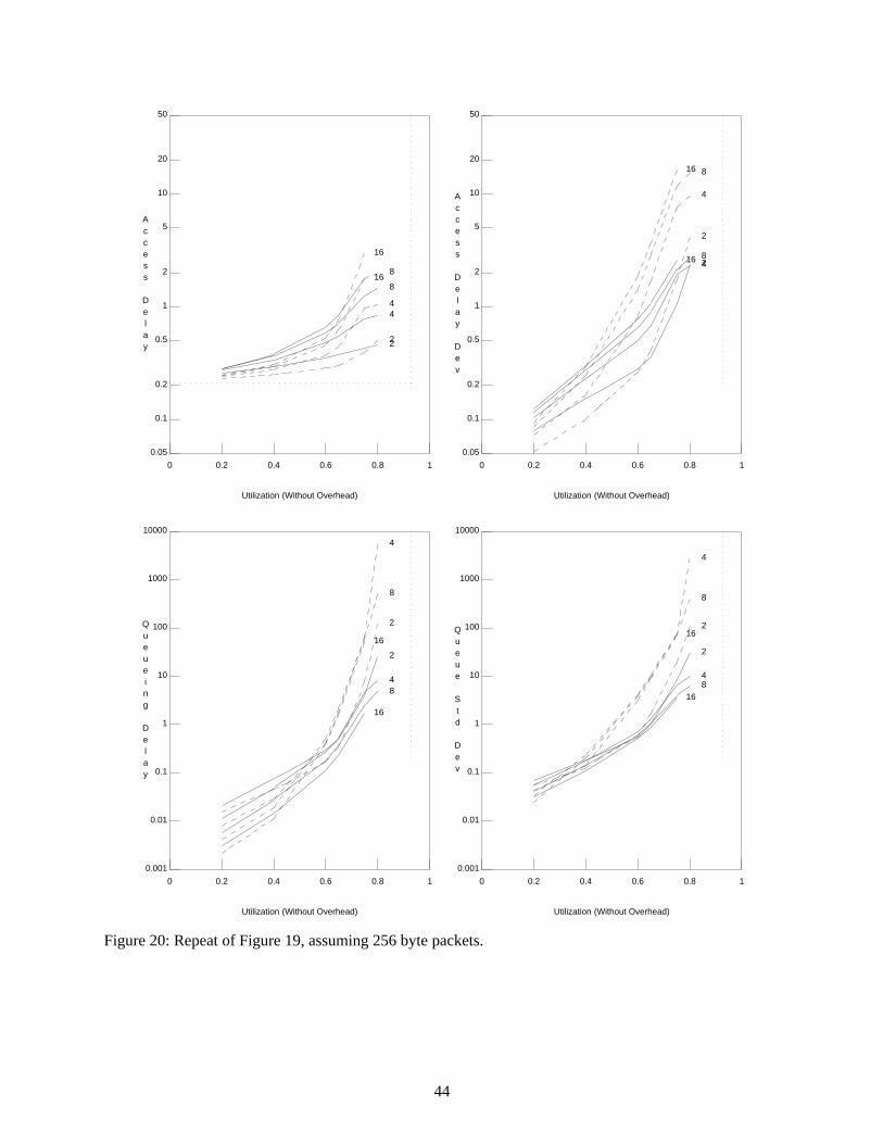
0.05

0.1

0.2

0.5

1

2

5

10

20

50

0 0.2 0.4 0.6 0.8 1


Access

Delay

. . . . . . . . . . . . . . . . . . . . . . . . . . . . . . . . . . . . . . . . . . . . . . .....................................................

2

4

8

16

2

4

816

0.05

0.1

0.2

0.5

1

2

5

10

20

50

0 0.2 0.4 0.6 0.8 1


Access

Delay

Dev

.

.

.

.

.

.

.

.

.

.

.

.

.

.

.

.

.

.

.

.

.

.

.

.

.

.

.

.

.

.

.

.

.

.

.

.

.

.

.

.

.

.

.

.

.

.

.

.

.

.

.

.

2

4

816

24816

0.001

0.01

0.1

1

10

100

1000

10000

0 0.2 0.4 0.6 0.8 1


Queueing

Delay

.

.

.

.

.

.

.

.

.

.

.

.

.

.

.

.

.

.

.

.

.

.

.

.

.

.

.

.

.

.

.

.

.

.

.

.

.

.

.

.

.

.

.

.

2

4

8

16

2

48

16

0.001

0.01

0.1

1

10

100

1000

10000

0 0.2 0.4 0.6 0.8 1


Queue

Std

Dev

.

.

.

.

.

.

.

.

.

.

.

.

.

.

.

.

.

.

.

.

.

.

.

.

.

.

.

.

.

.

.

.

.

.

.

.

.

.

.

.

.

.

.

.

2

4

8

16

2

48

16

Figure 20: Repeat of Figure 19, assuming 256 byte packets.

44

0.02

0.05

0.1

0.2

0.5

1

2

5

10

20

0 0.2 0.4 0.6 0.8 1


Access

Delay

. . . . . . . . . . . . . . . . . . . . . . . . . . . . . . . . . . . . . . .........................................................

2

4

816

2

4

816

0.02

0.05

0.1

0.2

0.5

1

2

5

10

20

0 0.2 0.4 0.6 0.8 1


Access

Delay

Dev

.

.

.

.

.

.

.

.

.

.

.

.

.

.

.

.

.

.

.

.

.

.

.

.

.

.

.

.

.

.

.

.

.

.

.

.

.

.

.

.

.

.

.

.

.

.

.

.

.

.

.

.

.

.

.

.

2

4

8

16

248

16

0.001

0.01

0.1

1

10

100

1000

10000

0 0.2 0.4 0.6 0.8 1


Queueing

Delay

.

.

.

.

.

.

.

.

.

.

.

.

.

.

.

.

.

.

.

.

.

.

.

.

.

.

.

.

.

.

.

.

.

.

.

.

.

.

.

.

.

.

.

.

.

.

.

.

.

.

2

4

8

162

4

8

16

0.001

0.01

0.1

1

10

100

1000

10000

0 0.2 0.4 0.6 0.8 1


Queue

Std

Dev

.

.

.

.

.

.

.

.

.

.

.

.

.

.

.

.

.

.

.

.

.

.

.

.

.

.

.

.

.

.

.

.

.

.

.

.

.

.

.

.

.

.

.

.

.

.

.

.

.

.

2

4

8

162

4

8

16

Figure 21: Repeat of Figure 19, assuming 64 byte packets.

45

significantly busy, then the effects of the MAC layer deferrals and backoffs will distort the arrival patternsignificantly. Furthermore, any performance statistics obtained by using such a trace to drive a networksimulator would be extremely misleading: a network faced with a trace of its own (already scheduled)departure process would experience no collisions and no queueing delays. Thus, our solution was to dis-card all traces whose average utilization over the hour was more than 0.10 (to reduce the distortionscaused by MAC layer deferrals and backoffs), and then overlay multiple traces to construct an aggregatetrace having the desired load. Obviously this is not perfect, but it is certainly much more realistic than asimple Poisson model.

Before launching into a whole new set of results that were obtained using this trace-driven simu-lation methodology, we first need to establish that this approach does indeed give us a much better pictureof the behaviour of a typical Ethernet system than the simple Poisson model. Thus, we will now showthat this trace-driven simulation methodology is good enough to preserve most of the details of the accessdelay distribution information. In Figure 22, we have shown three complete sets of collision retry data,where each set shows the equivalent information to Figure 10 for a different system. In part (a) of theFigure, the raw data was obtained using the same locally-built hardware monitor that we used in Figure10, but this time it is connected to another host (the author’s Sun SPARCstation 2 workstation), which isconnected to another Ethernet. Nevertheless, the two sets of data exhibit many similarities, and it is nothard to believe that the data was obtained in the same way.

In part (b) of the Figure, the raw data was obtained by instrumenting our simulator to record thesame information for all hosts that our hardware monitor supplies for a single host. The simulator wasrun for 1 hour of simulated time, using a trace-driven input file to load the network to an averagethroughput of approximately 2 Mbit/sec. Once again, the new data set is qualitatively very similar to thetwo earlier sets of data, and appears to have been obtained in the same way. Thus, we feel quite justifiedin assigning a high degree of credibility to the measurements we obtain using this trace driven simulationapproach.

On the other hand, the data shown in part (c) of the Figure is obviously very different from theothers. As in part (b), the raw data was generated using our trace-driven simulation methodology, andindeed we even re-used the exact same trace-driven input file and the same random number seeds. Theonly change we made was to modify the MAC layer state machine in each host to use BLAM instead ofBEB. By comparing parts (b) and (c) of Figure 22, we can that changing the backoff algorithm has asignificant effect on all three of the collision retry curves. First, the ‘‘tail’’ of the access delay distribu-tion, F (x), is much shorter, with the probability that a packet is still in the system falling off quitedramatically beyond 12,000 bits (which is the channel holding time limit under BLAM). Second, condi-tional retransmission attempt rate, G (x), is essentially constant for large values of x (rather than decreas-ing like the function Pn) after we account for the peaks caused by deferrals.18 And, finally, the conditionalprobability of success at each attempt, S (x), can be seen to be more stable under BLAM than under BEB.The drop near 12,000 bit times (i.e., the channel holding time) happens because the number of activehosts and the length of the resulting busy period are positively correlated.

¼ ¼�¼�¼�¼�¼�¼�¼�¼�¼�¼�¼�¼�¼�¼18 The fact that G (x) appears to be bounded between 10−4 and 10−3 can be explained by recognizing that, underBLAM, each active host makes an average of one transmission attempt per ‘‘cycle’’ (because CCounter isinitialized to 1, about 1/2 of the active hosts transmit in the first contention slot; if there is a collision, then about 1/4of the active hosts transmit in the second contention slot, etc., and 1/2 + 1/4 + 1/8 + . . . = 1) and the average lengthof a ‘‘cycle’’ is roughly on the order of 103 (if the ‘‘winning’’ host sends a single short packet) to 104 (if the‘‘winning’’ host uses its full channel holding time) bits.

46

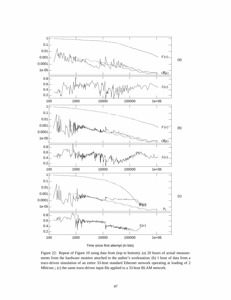
1

0.1

0.01

0.001

0.0001

1e-05

(a)F (x)

G (x)

.......................................... . ..... . . ........... ... ..................... . ................................. ........................ .......................... .......................... ................................. Pn

100 1000 10000 100000 1e+06

0.2

0.4

0.6

0.8

S (x)

1

0.1

0.01

0.001

0.0001

1e-05

(b)F (x)

G (x)

.......................................... . ..... . . ........... ... ..................... . ................................. ........................ .......................... .......................... ................................. Pn

100 1000 10000 100000 1e+06

0.2

0.4

0.6

0.8

S (x)

1

0.1

0.01

0.001

0.0001

1e-05

(c)

F (x)G (x)

.......................................... . ..... . . ........... ... ..................... . ................................. ........................ .......................... .......................... ................................. Pn

Time since first attempt (in bits)

100 1000 10000 100000 1e+06

0.2

0.4

0.6

0.8

S (x)

Figure 22: Repeat of Figure 10 using data from (top to bottom): (a) 20 hours of actual measure-ments from the hardware monitor attached to the author’s workstation; (b) 1 hour of data from atrace-driven simulation of an entire 33-host standard Ethernet network operating at loading of 2Mbit/sec.; (c) the same trace-driven input file applied to a 33-host BLAM network.

47

0.2

0.5

1

2

0 0.2 0.4 0.6 0.8 1


Access

Delay

....

....

....

....

....

.......... .

. .. .

. .. .

.. .. .

. .. .

..................................

....

... ..

....

.... BEB

....

....

....

....

............ . . . . . . .

. .. . . . . . .BLAM

0.2

0.5

1

2

5

10

20

0 0.2 0.4 0.6 0.8 1


Access

Std

Dev

....

....

....

....

....

...... . . . . . . . . .. . . . . . .

....

....

....

....

....

....... . . . . . . . . .. . . . . . . BEB

. . . . . . . . . . . . . .... . . . . . . .. . . . . . .BLAM

0.01

0.1

1

10

100

1000

0 0.2 0.4 0.6 0.8 1


Queueing

Delay

....

....

....

....

.... . . . . . . .

. .....

....

.

....

....

....

....

.... . . . . . . .

. .....

....

. BEB

. .. .

. .. .

. .. .

. .. . ...... .

. .. .

. .. .

.. . . . . . .BLAM

0.01

0.1

1

10

100

1000

0 0.2 0.4 0.6 0.8 1


Queue

Std

Dev

. . . . . . . . . . . . . . . .... . . . . . . . . .....

....

.

. . . . . . . . . . . . . . . .... . . . . . . . . .....

....

. BEB

. .. . .

. . .. .

. .. .

. ........ . . . . . . . . .. . . . . .BLAM

Figure 23: Comparison of the Mean and Standard Deviation of the Access Time and QueueingDelay between the Standard Ethernet and the Binary Logarithmic Backoff Method, using a 33-Host system with trace-driven packet sizes and interarrival times. Three replications of the exper-iment are shown. Dashed lines indicate a system where every host uses the standard EthernetBEB algorithm. Solid lines indicate a system where every host uses the BLAM algorithm. Thethree dotted lines indicate a mixed system, where hosts 0−15 use BEB and hosts 16−32 useBLAM: unlabelled curve shows the overall quantities, while the labelled curves show the resultsseparately for the two host types.

Figures 23 and 24 show the effects of introducing trace-driven traffic into the type of experimentreported in Figures 14−16 and 19−21 Each Figure displays the results from three separate experimentsusing the same trace-driven inputs: the dashed lines represent a system where all hosts use BEB, the solidlines represent a system where all hosts use BLAM, and the dotted lines represent a heterogeneous systemwhere some hosts use BEB and the rest use BLAM. Notice that in both 33-Host (Figure 23) and 4-Host(Figure 24) configurations, BLAM significantly outperforms BEB, and that adding some BLAM hostsonce again improves the performance of the BEB hosts in a mixed environment.

48

0.2

0.5

1

2

0 0.2 0.4 0.6 0.8 1


Access

Delay

. .. .

. .. .

. .. .

. .. .

. .. .

. ... . . . .. . . . .. . . . . . . . .

....

... .

... .

....

... .

. .... . . . .. . . . .. .

. .. .

. .. .

. BEB

. .. .

. .. .

. .. .

. .. .

. .. .

. .. . . . . .. . . . .. . . . . . . .BLAM

0.2

0.5

1

2

5

10

20

0 0.2 0.4 0.6 0.8 1


Access

Std

Dev ..

....

. ...

. ...

....

. .. .

... . . . .. . . . .. . . . . . . . .

....

....

....

....

....

....

... . . . .. . . . .. . . . . . . . . BEB

. . . . . . . . . . . . . . . . . .. . . . .. . . . .. . . . . . . .BLAM

0.1

1

10

100

1000

10000

0 0.2 0.4 0.6 0.8 1


Queueing

Delay

....

....

....

....

....

....

.. . . . .....

..................

....

....

....

....

....

....

.... . . . ...

....

................ BEB

. .. .

. .. .

. .. .

. .. .

. .. .

. ... . . . . .. . . . ...

...................BLAM

0.1

1

10

100

1000

10000

0 0.2 0.4 0.6 0.8 1


Queue

Std

Dev ..

....

. ...

. ...

....

. .. .

... . . . .. . .. .

.....

....

....

.

....

... .

... .

....

... .

. .... . . . .. . .

. ....

....

....

... BEB

. .. .

. .. .

. .. .

. .. .

. .. .

. ............ . . . ...

.....................BLAM

Figure 24: Repeat of Figure 23 using a 4-Host trace driven experiment. Dashed lines indicate arun using only BEB hosts, solid lines indicate a run using only BLAM hosts, and dotted lines indi-cate a mixed configuration.

Figures 25−28 provide more details about the grade of service experienced by the individualhosts. Here each point represents the performance of a single host at a single experiment, with the emptycircles representing hosts using BEB and the solid circles representing hosts using BLAM. Figures 25and 26 each show the change in performance that results from switching all hosts from BEB to BLAM attwo different values of total utilization. Figure 27 shows the same setup as in Figure 25, but with half thehosts using BEB and the other half using BLAM. Figure 28 shows the corresponding results for a 4-Hostconfiguration.

49

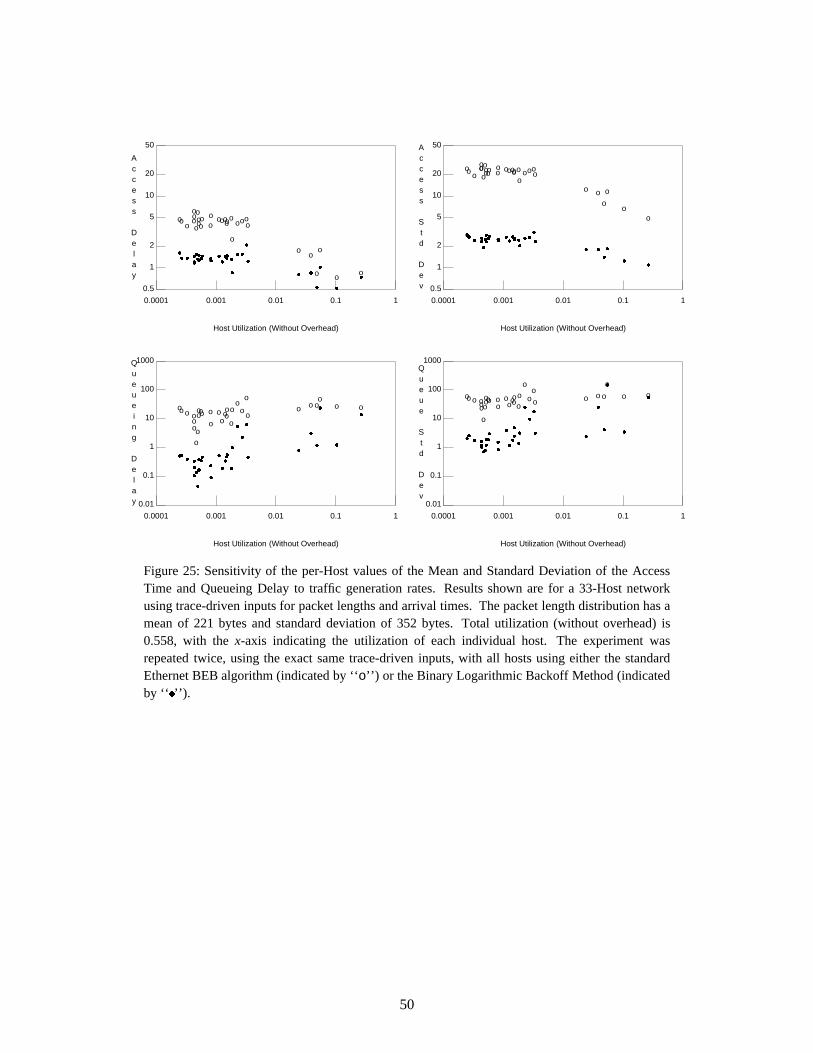
0.5

1

2

5

10

20

50

0.0001 0.001 0.01 0.1 1

Host Utilization (Without Overhead)

Access

Delay ½

½ ½½½ ½½ ½½½

½ ½ ½ ½½ ½½ ½½½ ½½ ½ ½ ½½ ½½½ ½½o

o

o

oo

o

o

o

o

o

o o ooo

o

o

o

ooo

ooo

oo ooo oo

0.5

1

2

5

10

20

50

0.0001 0.001 0.01 0.1 1


Access

Std

Dev

¾¾ ¾¾¾ ¾¾ ¾¾¾

¾ ¾ ¾ ¾¾ ¾¾ ¾¾¾ ¾¾ ¾ ¾ ¾¾ ¾¾¾ ¾¾

o

o

o

oo

o

o

o

o

o

o o o oo

oo

o

ooo

ooo oo ooo oo

0.01

0.1

1

10

100

1000

0.0001 0.001 0.01 0.1 1


Queueing

Delay

¿¿ ¿¿¿

¿

¿¿¿ ¿¿ ¿ ¿ ¿¿ ¿¿

¿¿¿ ¿¿ ¿ ¿

¿¿ ¿¿¿

¿¿o

oo

o

o

o

o

oo oo oo

oooo

ooo

oo

oo

oo

o

oo oo

0.01

0.1

1

10

100

1000

0.0001 0.001 0.01 0.1 1


Queue

Std

Dev

ÀÀ ÀÀÀ

À

ÀÀÀ

ÀÀ À À ÀÀ ÀÀÀ

ÀÀ ÀÀ À ÀÀ

À ÀÀÀÀÀ

oo oo

o

o

oo

o

oo oo oo

oo

oooo

ooo

oo

ooo oo

Figure 25: Sensitivity of the per-Host values of the Mean and Standard Deviation of the AccessTime and Queueing Delay to traffic generation rates. Results shown are for a 33-Host networkusing trace-driven inputs for packet lengths and arrival times. The packet length distribution has amean of 221 bytes and standard deviation of 352 bytes. Total utilization (without overhead) is0.558, with the x-axis indicating the utilization of each individual host. The experiment wasrepeated twice, using the exact same trace-driven inputs, with all hosts using either the standardEthernet BEB algorithm (indicated by ‘‘o’’) or the Binary Logarithmic Backoff Method (indicatedby ‘‘Á ’’).

50

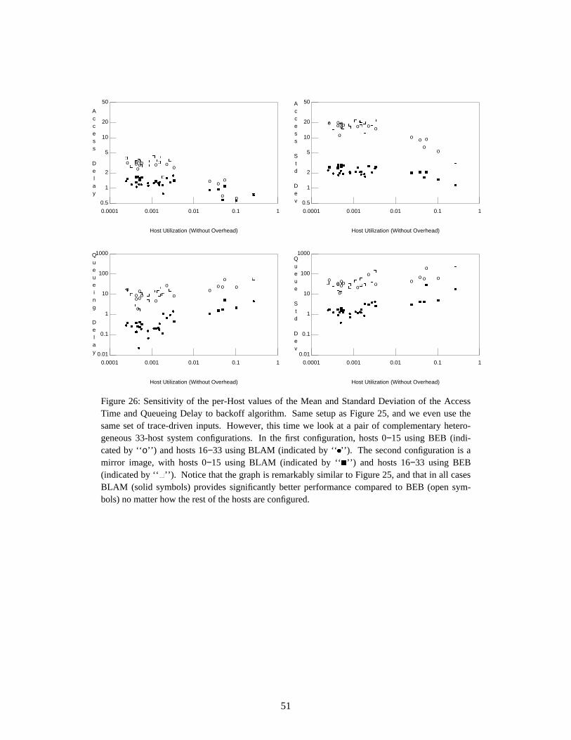
0.5

1

2

5

10

20

50

0.0001 0.001 0.01 0.1 1


Access

Delay o

o

o

oo

o

o

o

o

o

o oo o

o

ÂÂ ÂÂÂ ÂÂ Â Â ÂÂ ÂÂÂ ÂÂÃ

ÃÃ

Ã Ã Ã ÃÃ ÄÄ

ÄÄ

ÃÄ ÄÄ Ä Ä ÄÄ ÄÄÄ ÄÄÃÃ ÃÃ ÃÃ

0.5

1

2

5

10

20

50

0.0001 0.001 0.01 0.1 1


Access

Std

Dev

o

o

o

o

oo

o

o

o

o

o o o oo

ÅÅ ÅÅÅ ÅÅ Å Å ÅÅ ÅÅÅ ÅÅ ÆÆ ÆÆ Æ Æ ÆÆÇÇ

ÇÇ

Æ

Ç ÇÇ Ç Ç ÇÇ ÇÇÇ ÇÇÆÆ ÆÆ ÆÆ

0.01

0.1

1

10

100

1000

0.0001 0.001 0.01 0.1 1


Queueing

Delay

o

oo

o

o

o

o

oo oo o

ooo

ÈÈÈ

ÈÈ ÈÈ ÈÈ

ÈÈ ÈÈÈÈÈ

ÉÉ

ÉÉ É É ÉÉ

ÊÊÊ

ÊÉ

Ê ÊÊ Ê ÊÊÊ ÊÊÊ ÊÊ

ÉÉÉ

ÉÉÉ

0.01

0.1

1

10

100

1000

0.0001 0.001 0.01 0.1 1


Queue

Std

Dev

oo

oo

o

o

ooo

oo oo oo

ËËË

ËË ËË Ë ËËË ËËË ËË ÌÌ ÌÌ Ì Ì ÌÌ

ÍÍÍ

ÍÌ

Í ÍÍ Í ÍÍÍ ÍÍÍ ÍÍ

ÌÌÌ

Ì ÌÌ

Figure 26: Sensitivity of the per-Host values of the Mean and Standard Deviation of the AccessTime and Queueing Delay to backoff algorithm. Same setup as Figure 25, and we even use thesame set of trace-driven inputs. However, this time we look at a pair of complementary hetero-geneous 33-host system configurations. In the first configuration, hosts 0−15 using BEB (indi-cated by ‘‘o’’) and hosts 16−33 using BLAM (indicated by ‘‘Î ’’). The second configuration is amirror image, with hosts 0−15 using BLAM (indicated by ‘‘Ï ’’) and hosts 16−33 using BEB(indicated by ‘‘Ð ’’). Notice that the graph is remarkably similar to Figure 25, and that in all casesBLAM (solid symbols) provides significantly better performance compared to BEB (open sym-bols) no matter how the rest of the hosts are configured.

51

0.5

1

2

5

10

20

50

0.0001 0.001 0.01 0.1 1


Access

Delay Ñ

ÑÑ

Ñ ÑÑ ÑÑÑ

ÑÑ Ñ ÑÑÑÑ

ÑÑÑ ÑÑ ÑÑ ÑÑ ÑÑ ÑÒÑÑ

o

o

o

o

o

o

o

o

o

oo oo

o

o

o

o

oooo oo

o

oo

oo oo

0.5

1

2

5

10

20

50

0.0001 0.001 0.01 0.1 1


Access

Std

Dev

ÓÓ ÓÓ ÓÓ ÓÓ

ÓÓÓ Ó ÓÓ ÓÓ

ÓÓÓ ÓÓ ÓÓ ÓÓ ÓÓ Ó ÓÓ

o

o

o

o

o

o

o

o

o

oo o oo

oo

o

oooo oo

o

o oo o oo

0.1

1

10

100

1000

0.0001 0.001 0.01 0.1 1


Queueing

Delay

ÔÔ

ÔÔÔ

ÔÔ

ÔÔ

ÔÔ Ô ÔÔ ÔÔ

Ô

ÔÔ ÔÔ ÔÔ

ÔÔ ÔÔ Ô ÔÔ

oo oo

o

o

oo

oo

o o oo o

o

o

ooo

oo

o

oo

oo o oo

0.1

1

10

100

1000

0.0001 0.001 0.01 0.1 1


Queue

Std

Dev

ÕÕ

ÕÕÕ

Õ

Õ

ÕÕ

ÕÕ ÕÕÕ ÕÕ

Õ

ÕÕ ÕÕ ÕÕÕ

Õ ÕÕ Õ ÕÕo

o oo

o

oo

oo

oo

ooo o

o

o

oooo o

o

oo oo o oo

Figure 27: Repeat of Figure 25 in a saturated 33-Host network. Total utilization (without over-head) is 0.655, and the packet length distribution has a mean of 220 bytes and standard deviationof 344 bytes. The experiment was repeated twice, using the exact same trace-driven inputs, withall hosts using either the standard Ethernet BEB algorithm (indicated by ‘‘o’’) or the Binary Loga-rithmic Backoff Method (indicated by ‘‘Ö ’’).

52

0.2

0.5

1

2

5

10

20

0.01 0.02 0.05 0.1 0.2 0.5 1


Access

Delay ×

× × ×o

o

oo

0.2

0.5

1

2

5

10

20

0.01 0.02 0.05 0.1 0.2 0.5 1


Access

Std

Dev

ØØ Ø Ø

o

o

o o

1

10

100

1000

0.01 0.02 0.05 0.1 0.2 0.5 1


Queueing

Delay

ÙÙ Ù

Ùoo o o

1

10

100

1000

0.01 0.02 0.05 0.1 0.2 0.5 1


Queue

Std

Dev

Ú

Ú Ú

Úoo oo

Figure 28: Repeat of Figure 25 for a trace-driven 4-host system configuration in which the totalutilization (without overhead) is 0.638 and the packet size distribution has a mean of 196 bytesand standard deviation of 305 bytes. Data for two experimental runs is shown, with BEB indi-cated by ‘‘o’’ and BLAM indicated by ‘‘Û ’’.

V. Implementation Considerations

Most of the advantages of BLAM over BEB come from deriving more information about thestate of the network from the available signals coming into the host interface from the attached mediumaccess unit (i.e., transceiver). Thus, to demonstrate the viability of BLAM, we must show that this infor-mation is indeed available, and at little or no additional implementation complexity compared to BEB.

The primary distinction between BLAM and BEB in terms of signalling is the use of ternary (i.e,idle / success / collision) state information about the channel. Obviously, carrier sensing can be used todistinguish an idle channel from a busy one, since this is how the deference process is defined. Further-more, if the given host is actively transmitting, then collision detection can be used to distinguish a suc-cess from a collision, using either analog voltage levels on shared media (i.e., 10Base5 and 10Base2) ordigital logic on unidirectional point-to-point channels (simultaneous, non-loopback transmission andreception on twisted pair or optical fibre). Thus, it remains to show how a passive observer can easilydistinguish between a success or collision in which it was never involved. Our solution consists of classi-fying such a period of activity as a collision if and only if its duration in bits, after discounting the pream-ble, is less than the minimum frame length of 512 bits. Notice that this involves little additional work onthe part of the host, since this same test is used for filtering collision fragments before passing frames to

53

the host interface. Furthermore, it does not require decoding the frame in any way, including theverification of the frame CRC.

Our method of enforcing a channel holding time limit in a distributed way uses the constantBurstSpace (measured in bits) to indicate whether or not a successful host wishes to continue to sendmore packets in the same transmission burst. The value of BurstSpace is based on the fact that the inter-frame spacing between two consecutive packets originating from the same source can change by at most47 bit times because of the variability of carrier acquisition at repeaters, etc., in the worst-case transmis-sion path. Doubling that value provides us with a simple test to determine whether or not the host thatsent the previous packet intends to send another one. That is, if that host transmits its next packet within48 bit times of a nominal interFrameGap — which is well within the capabilities of most current works-tations — then all other hosts will detect a start-of-carrier event before their BurstSpace timeout expiresand hence will not interfere with the successful host.

We believe that the idea of introducing the concept of a channel holding time to improveefficiency in the presence of short packets is an important contribution of this work. Thus, we stronglyrecommend that every implementation of a network interface that supports BLAM should contain at least3KBytes of local buffering for both transmission and reception, which is sufficient to hold all the data thata host is allowed to transmit during a single transmission burst. Thus, even if the host cannot support ahigh throughput rate on a sustained basis (because either the processing speed of the attached host or thehost-interface data transfer rate is a bottleneck), it can still take full advantage of BLAM.

Often, the price of efficiency is a loss of robustness in the face of errors, or perhaps some addedcomplexity in the rules for allowing new hosts to join a running network or existing hosts to leave. InBLAM, we made a significant effort to make the algorithm resilient to such problems. In particular, thealgorithm is designed to work correctly in a heterogeneous environment in which some of the hosts areusing the standard Ethernet BEB algorithm.

Thus, a new host wishing to join the network can do so immediately, merely by acting like a stan-dard Ethernet host. If it arrives during an idle period on the network, then it will immediately becomesynchronized with the global state of the algorithm. If it arrives during an arbitration period, then it willimmediately become almost synchronized with the global algorithm: the only missing piece of informa-tion is the correct value of CCounter, which in general may be greater than 1 at this point. Although thenew host may enjoy a temporary advantage during this arbitration period because of its low value ofCCounter, it will acquire the correct value as soon as the first successful transmission occurs. And,finally, if it arrives during some other host’s transmission burst, then it will cause a collision to occur andall other hosts will follow it into the beginning of a new arbitration period.

Similarly, the departure of an existing host — even if it crashes during the arbitration period, orpart way through its transmission burst — has virtually no effect on the other hosts. In the former case,its transmission attempts may have caused CCounter at the other hosts to grow unnecessarily large.However, it will recover at the rate of one step per MaxIdle, and when we reach CCounter = 1 we are sureto transmit any remaining packet(s) within two slot times. Conversely, in the latter case, such a failure isno different than the successful host running out of packets to send, so all will be back to normal withinBurstSpace.

Finally, various physical layer transmission error conditions create no significant additional prob-lems under BLAM, in comparison to standard Ethernet using BEB. For example, an excessively longcollision will cause the non-participating hosts to enter the SawSuccess state. If none of the participantsretransmits immediately, then one BurstSpace later the non-participants will reenter the arbitration phase(but with CCounter = 1 instead of CCounter > 1 for the participants in the long collision) and most likelyone of the non-participants will acquire the network. After the end of the successful host’s transmission

54

burst, all active hosts (including the ones responsible for the excessively long collision) will reenter thearbitration phase. However, since the minimum value of CCounter is unity, the same long collision is notnecessarily going to occur again.

VI. Conclusions

In this paper, we have described several major performance problems caused by the truncatedBinary Exponential Backoff (BEB) algorithm that is part of the Ethernet standard. These problems do notinterfere with the ultimate capacity of the network, defined as the maximum sustainable throughputwithout regard to delay. However, they can cause significant degradation of the users’ view of the serviceprovided by the network, as shown by the large and extremely unpredictable delays that can occur undermoderate to heavy traffic conditions. These delay anomalies can be severe enough to interfere with typi-cal networking applications, to the point where Ethernet may be labelled as uncompetitive with othertechnologies.

To solve these performance problems, we have developed a new backoff algorithm called theBinary Logarithmic Arbitration Method (BLAM), which eliminates all of these performance anomalieswithout introducing any new problems of its own. That is, we show that BLAM offers several significantadvantages over BEB, and indeed that switching to the new algorithm never causes any harm to systemperformance. BLAM does not reduce the ultimate capacity of the network compared to BEB. BLAMenjoys a dramatic delay advantage over BEB under moderate to high load conditions. BLAM is evenbackwards compatible with BEB in the sense that different hosts using both backoff algorithms can hap-pily coexist on the same network. Indeed, adding some BLAM hosts to an existing system actuallyimproves the performance of BEB hosts in almost all cases.

In a very real sense, Ethernet is on its way to becoming the Fortran of the 90’s: a pioneeringeffort to harness new technology that isn’t perfect but gets the job done — and refuses to go away in spiteof the introduction of a succession of new and improved alternatives. However, we should note that alarge part of Fortran’s longevity is due to the continuing efforts of its supporters to incorporate new ideas(such as recursion, pointers, and modules [2]), instead of simply making do with its original features, likesuch antediluvian control structures as the arithmetic IF and computed GOTO statements.

At the present time, Ethernet shows every indication that it will outlast all of its competitors andmost of its supposed successors. There is now a tremendous installed base of Ethernet compatible equip-ment in the world, which people are unwilling to discard without good reason. However, we believe thatit is inevitable that the performance anomalies in BEB will soon cause the momentum of Ethernet to belost, especially in the emerging higher speed market. Thus it is important to solve these problems now,by updating the MAC layer protocol to allow the use of the BLAM algorithm.

Acknowledgments — The author gratefully acknowledges the contribution of Wayne Hayes to this pro-ject, without whose efforts there would have been no simulation experiments for me to report in thispaper. The Computing Disciplines Facility of the Department of Computer Science at the University ofToronto provided both massive amounts of low priority CPU time on their cluster of Sun SPARCstationworkstations (on the order of CPU-years!) for running simulation experiments, and the source for thedata used in our trace-driven simulation experiments. This research was supported by the Natural Sci-ences and Engineering Research Council of Canada, under grant #A5517, and by the Information Tech-nology Research Centre of the Province of Ontario, Canada.

55

References

[1] ‘‘Carrier Sense Multiple Access with Collision Detection (CSMA/CD),’’ IEEE Std 802.3-1990Edition (ISO/DIS 8802-3), IEEE, New York (1990).

[2] J. C. Adams, W. S. Brainerd, J. T. Martin, B. T. Smith, and J. L. Wagener, Fortran 90 Handbook:Complete ANSI / ISO Reference, Intertext McGraw-Hill (1992).

[3] D. J. Aldous, ‘‘Ultimate Instability of Exponential Back-Off Protocol for Acknowledgement-Based Transmission Control of Random Access Communication Channels,’’ IEEE Transactionson Information Theory IT-33(2), pp. 219-223 (March 1987).

[4] G. T. Almes and E. D. Lazowska, ‘‘The Behavior of Ethernet-Like Computer CommunicationNetworks,’’ Proc. 7th Symposium on Operating Systems Principles, pp.66-81 (1979).

[5] S. Armyros, ‘‘On the Behaviour of Ethernet: Are Existing Analytic Models Adequate?,’’ Techni-cal Report CSRI-259, Computer Systems Research Institute, University of Toronto, Toronto(February 1992). (M.Sc. thesis).

[6] D. R. Boggs, J. C. Mogul, and C. A. Kent, ‘‘Measured Capacity of an Ethernet: Myths and Real-ity,’’ ACM SIGCOMM ’88 Symposium on Communications Architectures & Protocols, pp.222-234 (August 16-19, 1988).

[7] D. E. Comer, Internetworking with TCP/IP Vol I: Principles, Protocols, and Architecture,Prentice-Hall (1991). (Second Edition).

[8] R. W. Conway, W. L. Maxwell, and L. W. Miller, Theory of Scheduling, Addison-Wesley (1967).

[9] G. A. Cunningham and J. S. Meditch, ‘‘Distributed Retransmission Controls for Slotted, Nonper-sistent, and Virtual Time CSMA,’’ IEEE Transactions on Communications COM-36(6), pp.685-691 (June 1988).

[10] G. Fayolle, E. Gelenbe, and J. Labetoulle, ‘‘Stability and Optimal Control of the Packet SwitchingBroadcast Channel,’’ Journal of the ACM 24(3), pp.375-386 (July 1977).

[11] P. Gburzynski and P. Rudnicki, The SMURPH Protocol Modelling Environment (version 1.12),Department of Computing Science, University of Alberta, Edmonton (October 1991).

[12] J. Goodman, A. G. Greenberg, N. Madras, and P. March, ‘‘Stability of Binary Exponential Back-off,’’ Journal of the ACM 35(3), pp.579-602 (July 1988).

[13] R. Gusella, ‘‘A Measurement Study of Diskless Workstation Traffic on an Ethernet,’’ IEEE Tran-sactions on Communications 38(9) (September 1990).

[14] B. Hajek and T. van Loon, ‘‘Decentralized Dynamic Control of a Multiaccess Broadcast Chan-nel,’’ IEEE Transactions on Automatic Control AC-27(3), pp.559-569 (June 1982).

[15] V. Jacobson, ‘‘4BSD TCP Ethernet Throughput,’’ Internet Newsgroup Comp.protocols.tcp-ip(October 24, 1988). 139 lines.

[16] J. F. C. Kingman, ‘‘The Effect of Queue Discipline on Waiting Time Variance,’’ Proceedings ofthe Cambridge Philosophical Society 58, pp.163 - 164 (1962).

[17] L. Kleinrock, Queueing Systems, Volume II: Computer Applications, Wiley-Interscience, NewYork (1976).

56

[18] A. Leon-Garcia, Probability and Random Processes for Electrical Engineering, Addison-Wesley,Reading, MA (1989).

[19] J. L. Massey, ‘‘Guest Editorial,’’ IEEE Transactions on Information Theory IT-31(2), pp. 117-118 (March 1985).

[20] J. S. Meditch and C. A. Lea, ‘‘Stability and Optimization of the CSMA and CSMA/CD Chan-nels,’’ IEEE Transactions on Communications COM-31(6), pp. 763-774 (June 1983).

[21] R. M. Metcalfe and D. R. Boggs, ‘‘Ethernet: Distributed Packet Switching for Local ComputerNetworks,’’ Communications of the ACM 19(7) (July 1976).

[22] R. M. Metcalfe, ‘‘Computer/Network Interface Design: Lessons from Arpanet and Ethernet,’’IEEE Journal on Selected Areas in Communications SAC-11(2), p.173,180 (February 1993).

[23] M. L. Molle, K. Sohraby, and A. N. Venetsanopoulos,, ‘‘Space-Time Models of AsynchronousCSMA Protocols for Local Area Networks,’’ IEEE Journal on Selected Areas in CommunicationsSAC-5(6), pp.956-968 (July 1987).

[24] S. Shenker, ‘‘Some Conjectures on the Behavior of Acknowledgement-Based Transmission Con-trol of Random Access Communication Channels,’’ ACM SIGMETRICS ’87 Conference on Meas-urement and Modeling of Computer Systems,, pp.245-255 (May 1987).

[25] J. F. Shoch and J. A. Hupp, ‘‘Measured Performance of an Ethernet Local Network,’’ Communi-cations of the ACM 23(12), pp. 711-721 (December 1980).

[26] K. Sohraby, M. L. Molle, and A. N. Venetsanopoulos, ‘‘Comments on ‘Throughput Analysis forPersistent CSMA Systems’ ,’’ IEEE Transactions on Communications COM-35(2), pp.240-243(February 1987).

[27] J. D. Spraggins, J. L. Hammond, and K. Pawlikowski, Telecommunications: Protocols andDesign, Addison-Wesley (1991).

[28] H. Takagi and L. Kleinrock, ‘‘Throughput Analysis of Persistent CSMA Systems,’’ IEEE Tran-sactions on Communications COM-33, pp.627-638 (July 1985).

[29] A. S. Tanenbaum, Computer Networks, Prentice-Hall, Inc., Englewood Cliffs, N. J. (1988).(Second Edition).

[30] C. P. Thacker, E. M. McCreight, B. W. Lampson, R. F. Sproull, and D. R. Boggs, ‘‘Alto: A Per-sonal Computer,’’ pp. 549-572 in Computer Structures: Principles and Examples, ed. D. P.Siewiorek, C. G. Bell and A. Newell, McGraw-Hill (1982).

[31] R. Walsh and R. Gurwitz, ‘‘Converting the BBN TCP/IP to 4.2BSD,’’ Usenix 1984 SummerConference Proceedings, pp.52-61 (June 12−15, 1984).

[32] J. K. Wolf, ‘‘Born again Group Testing: Multiaccess Communications,’’ IEEE Transactions onInformation Theory IT-31(2), pp. 185-191 (March 1985).

[33] Z. Zilic and M. L. Molle, ‘‘Modelling the Exponential Backoff Algorithm in CSMA/CD Net-works,’’ Technical Report CSRI-279, Computer Systems Research Institute, University ofToronto, (October 1992).

57

a new binary logarithmic arbitration method for ethernet

Documents