Sensors 2018, 18, 2740; doi:10.3390/s18082740 www.mdpi.com/journal/sensors

Article

A New Approach to Unwanted-Object Detection in

GNSS/LiDAR-Based Navigation

Mathieu Joerger 1,*, Guillermo Duenas Arana 2, Matthew Spenko 2 and Boris Pervan 2

1 College of Aerospace & Mechanical Engineering, The University of Arizona, Tucson, AZ 85721, USA 2 Armour College of Engineering, Illinois Institute of Technology, Chicago, IL 60616, USA;

gdueasar@hawk.iit.edu (G.D.A.); mspenko@iit.edu (M.S.); pervan@iit.edu (B.P.)

* Correspondence: joerger@email.arizona.edu

Received: 21 June 2018; Accepted: 16 August 2018; Published: 20 August 2018

Abstract: In this paper, we develop new methods to assess safety risks of an integrated

GNSS/LiDAR navigation system for highly automated vehicle (HAV) applications. LiDAR

navigation requires feature extraction (FE) and data association (DA). In prior work, we established

an FE and DA risk prediction algorithm assuming that the set of extracted features matched the set

of mapped landmarks. This paper addresses these limiting assumptions by incorporating a Kalman

filter innovation-based test to detect unwanted object (UO). UO include unmapped, moving, and

wrongly excluded landmarks. An integrity risk bound is derived to account for the risk of not

detecting UO. Direct simulations and preliminary testing help quantify the impact on integrity and

continuity of UO monitoring in an example GNSS/LiDAR implementation.

Keywords: navigation; safety; GNSS; LiDAR; detection; integrity monitoring; autonomous cars

1. Introduction

This paper describes the design, analysis, and preliminary testing of a new method to quantify

safety in GNSS/LiDAR navigation systems. An integrity risk bound is derived, which accounts for

failures to detect undesirable, unmapped and wrongly extracted obstacles. The paper describes an

innovation-based method, which is an alternative to the solution separation approach used in [1]. In

addition, the paper provides the means to quantify the impact of unwanted objects (UO) on the risk

of incorrect association. This work is intended for driverless cars, or highly automated vehicles (HAV)

[2,3], operating in changing environments where unknown, moving obstacles (cars, buses, and

trucks) are not wanted as landmarks for localization, and may occlude other useful, mapped

landmarks.

This research leverages prior analytical work carried out in civilian aviation navigation where

safety is assessed in terms of integrity and continuity [4]. These performance metrics are sensor- and

platform-independent. Integrity is a measure of trust in sensor information: integrity risk is the

probability of undetected sensor errors causing unacceptably large positioning uncertainty [4].

Continuity is a measure of the navigation system’s ability to operate without unscheduled

interruption. Both loss of integrity and loss of continuity can place the HAV in hazardous situations

[4,5].

Several methods have been established to predict integrity and continuity risks in GNSS-based

aviation applications [6–8]. Unfortunately, the same methods do not directly apply to HAVs, because

ground vehicles operate under sky-obstructed areas where GNSS signals can be altered or blocked

by buildings and trees.

HAVs require sensors in addition to GNSS, including LiDARs, cameras, or radars. This paper

focuses on LiDARs because of their prevalence in HAVs, of their market availability, and of our prior

Sensors 2018, 18, 2740 2 of 17

experience. A raw LiDAR scan is made of thousands of data points, each of which individually does

not carry any useful navigation information. Raw measurements must be pre-processed before they

can be used to estimate HAV positioning and orientation (or pose).

A first class of algorithms establishes correlations between successive scans to estimate sensor

changes in ‘pose’ (i.e., position and orientation) [9–12]. These procedures, including the Iterative

Closest Point (ICP) approach [13], can become cumbersome when evaluating safety of HAVs moving

over time. A second class of algorithms provides sensor localization by tracking recognizable, static

features in the perceived environment (seminal references and survey papers can be found in [14–19]). Features can include, for example, lines or planes corresponding to building walls in two- or

three-dimensional scans, respectively. Previous knowledge of feature parameters can be provided

either from a landmark map, or from past-time estimation in Simultaneous Localization and

Mapping (SLAM) [15,20]. The resulting information can then be iteratively processed using

sequential estimators in SLAM (e.g., Extended Kalman filter or EKF), which is convenient in practical

implementations. To estimate the HAV’s pose starting from a raw LiDAR scan, two intermediary, pre-estimator procedures must be carried out: feature extraction (FE), and data association (DA).

First, FE aims at finding the few most consistently recognizable, viewpoint-invariant, and

mutually distinguishable landmarks in the raw sensor data. Second, DA aims at assigning the

extracted features to the corresponding feature parameters assumed in the estimation process, i.e., at

finding the ordering of mapped landmarks that matches the ordering of extracted features over

successive observations. Incorrect association is a well-known problem that can lead to large

navigation errors [21], thereby representing a threat to navigation integrity. FE and DA can be

challenging in the presence of sensor uncertainty. This is why many sophisticated algorithms have

been devised [17–19,21–23]. But, how can we prove whether FE and DA are safe for life-critical HAV

navigation applications?

This research question is mostly unexplored. Several publications on multi-target tracking

describe relevant approaches to evaluate the probability of correct association in the presence of

measurement uncertainty [24,25]. However, these algorithms are not well suited for safety-critical

HAV applications due to their lack of prediction capability, to approximations that do not necessarily

upper-bound risks, and to high computational loads. Also, the risk of FE is not addressed. Overall,

research on integrity and continuity of FE and DA is sparse.

This paper builds upon prior work in [1,26–28], where we developed an analytical integrity risk

prediction method using a multiple-hypothesis innovation-based DA process. We established a

compact expression for the integrity risk of LiDAR-based pose estimation over successive iterations.

However, references [26–28] made simplifying assumptions that limit the applicability of these prior

results. For example, we assumed that the set of landmarks in the a-priori map was exactly the same

as the one being extracted. This assumption was relaxed in [1] where we developed an integrity-risk-

minimizing data-selection method. To achieve this, we derived a bound on the risk of incorrect

association, with which a subset of measurements can be used while considering potential wrong

associations with all landmarks surrounding the LiDAR. This bound was used in a preliminary

approach to detect UO using solution separation tests. In practice, UO such as other vehicles passing

by are likely to be extracted, and may even occlude other mapped landmarks. Obstacle detection

methods have been developed to mitigate the impact of such UOs (example methods are described

in [29,30]). But, the safety risks of using UOs as landmarks for navigation have yet to be fully

quantified.

In response, in this paper, we derive new methods to quantify the integrity risk caused by

failures to detect unwanted obstacles (UO), while guaranteeing a predefined false alert risk

requirement.

Section 2 of the paper provides an overview of the risk evaluation methods developed in [1,26–28], and of their limitations. These methods use a nearest-neighbor DA criterion [9], defined by the

minimum normalized norm of the EKF innovation vectors over all possible landmark permutations.

Sections 3 and 4 deal with the situation where a mapped landmark is not extracted, but another

unknown obstacle is extracted instead (e.g., case of an obstacle masking a mapped landmark). This

Sensors 2018, 18, 2740 4 of 17

k is the standard deviation of the estimation error for the vehicle state of interest (or linear

combination of states);

2 { , }P dof T

is the probability that a chi-squared-distributed random variable with “dof” degrees of

freedom is lower than some value T;

ln is the number of measurements at time step l ;

lm is the number of estimated state parameters at time step l ;

,FE lI is an integrity risk budget allocation, i.e., a fraction of kREQI ,

that we choose to satisfy:

, ,FE k REQ kI I ; 2

lL is the minimum mean normalized separation between landmark features that can be

guaranteed with probability larger than ,1 FE lI− . The normalized feature separation

metric is derived in [28]. 2

lL is derived at FE using a map or database of landmarks or

using landmark observations at previous time-steps in SLAM; 2

l is a mapping coefficient from separation space to EKF innovation space. This coefficient

is determined by solving an eigenvalue problem in [28]. The minimum eigenvalue is

taken to lower bound ( )KP CA , which is conservative; 2 2

l lL forms a probabilistic lower bound on the mean innovation’s norm, which is further described in the Section 2.2.

The integrity risk bound in Equation (1) is refined in this paper to account for the presence of

UOs and for failures to detect them. Equation (1) captures a key tradeoff in data association: on the

one hand, using only few measurements can cause a large nominal estimation error and hence large

( | )k KP HMI CA ; but on the other hand, few measurements from sparsely distributed landmarks can

improve ( )KP CA because features are “separated”, distinguishable, and therefore can be robustly associated. )( kHMIP is unknown, but we can assess safety by comparing

kREQI , to the upper bound

given in Equations (1)–(3), where all terms are known.

2.2. Innovation-Based Data Association

Equation (1) is derived for an innovation-based DA process, which is further described in the

following paragraphs. Let Ln be the total number of visible landmarks and Fn the number of

estimated feature parameters per landmark. Feature parameters can include landmark position, size,

orientation, surface properties, etc. When using LiDAR only (we integrate GNSS in Section 5), the

total number of feature parameters within the visible landmark set is: k L Fn n n . We can stack the

actual (true) values of the extracted feature parameters for all landmarks in an 1kn vector kz . Let

kz be an estimate of kz . We assume that the cumulative distribution function of kz can be

bounded by a Gaussian function with mean kz and covariance matrix kV [31–33]. We use the

notation: ˆ ~ ( , )k k kNz z V .

The nonlinear measurement equation can be written in terms of the 1km state parameter

vector kx as

kkkk vxhz += )(ˆ (4)

where

kx includes vehicle pose parameters and may also include landmark feature parameters (for SLAM-

type approaches);

kv is the extracted measurement noise vector: ),(~ 1 knk N V0v , where ba0 is an ba matrix of

zeros.

The mean of kz is )( kkk xhz = . Equation (4) can be linearized about an estimate kx of kx :

Sensors 2018, 18, 2740 9 of 17

is a scalar search parameter (fault magnitude) that is varied to maximize the

integrity risk at each time k ;

,MAX kg is the worst-case failure mode slope (FMS) over all UO hypotheses, determined

using the method given in [35];

2

2{ , , }NCP dof T

is the probability that a noncentrally chi-squared distributed random variable with

“dof” degrees of freedom and noncentrality parameter 2 is lower than some value T; 2

kT . is a detection threshold set in accordance to a continuity risk requirement REQC in

Equation (11);

,MDE lI is an integrity risk budget allocation, i.e., a fraction of kREQI ,

, chosen to satisfy

, , .MDE k REQ kI I

5. Performance Analysis

In this section, example simulations and testing introduced in [26–28,40,41] are employed to

compare the ( )kP HMI bounds assuming no UOs in Equations (1)–(3) versus accounting for possible

UOs in Equations (21)–(23).

5.1. Direct Simulation: Vehicle Roving through a GNSS-Denied Area

This analysis investigated the safety performance of a GPS/LiDAR navigation system onboard a

vehicle roving through a forest-type environment. GPS signals were blocked by the tree canopy, and

low-elevation satellite signals did not penetrate under the trees. Tree trunks served as landmarks for

a two-dimensional LiDAR using a SLAM-type algorithm.

The measurement vector kz in Equation (4) was augmented with GPS code and carrier

measurements. The state vector kx was augmented to include an unknown GPS receiver clock bias

and carrier phase cycle ambiguities. Time-correlated GPS signals and nonlinear LiDAR data were

processed in a unified time-differencing EKF derived in [33,34]. The main simulation parameter

values are listed in Table 1, and a differential GPS measurement error model was used, which is fully

described in [41]. In this scenario, GPS and LiDARs essentially relayed each other with seamless

transitions from open sky through GPS-denied areas where landmarks were modeled as poles with

nonzero radii.

Table 1. Simulation parameters.

System Parameters Values

Standard deviation of raw LiDAR ranging measurement 0.02 m

Standard deviation of raw LiDAR angular measurement 0.5 deg

LiDAR range limit 20 m

GNSS and LiDAR data sampling interval 0.5 s

Standard deviation of raw GNSS code ranging signal 1 m

Standard deviation of raw GNSS carrier ranging signal 0.015 m

GNSS multipath correlation time constant 90 s

Vehicle speed 1 m/s

Alert limit ℓ 0.5 m

Integrity risk allocation for FE, IFE,k 10−9

Integrity risk allocation for MDE, IMDE,k 10−10

Continuity risk requirement, CREQ,k 10−3

As shown in Figures 2–4 and 6, we consistently employed the following yellow-green-blue color

code: the mission started with the vehicle operating in a GPS available area (yellow-shaded). Satellite

signals available during initialization enabled accurate estimation of cycle ambiguities, so that vehicle

positioning uncertainty did not exceed a few centimeters. Then, as the vehicle moved and crossed the

Sensors 2018, 18, 2740 10 of 17

GPS- and LiDAR-available area (green-shaded) and the LiDAR-only area (blue-shaded), seamless

variations in covariance were achieved. A detailed description of this simulation is given in [41]. In

this scenario, the likelihood of IA is high.

First, as shown in Figure 2, we assumed that no UO was present but IAs occurred. One indicator

of IA is displayed on the top of the upper left-hand-side (LHS) plot in Figure 2. It shows that the

actual cross-track positioning error (thick black line) versus distance travelled exceeded the

corresponding one-sigma covariance envelope (thin black line). This suggests that errors impacting

positioning are not captured by the covariance.

This is confirmed on the lower part of the upper LHS chart in Figure 2, where the black curve

showing the ( | )k KP HI CA bound stayed below 710− . This curve can directly be derived from the

EKF covariance. It does not account for IA. In contrast, the red ( )kP HI -bound curve reached a first

plateau of ,FE kI = 10−9 as soon as two landmarks were visible by design of our risk evaluation method

[28]. The ( )kP HI curve then suddenly increased to 10−5 at approximately 29 m of travel distance.

To explain this sudden jump, the top right-hand-side (RHS) chart in Figure 2 shows that, at the

travel distance of 29 m (i.e., at travel time = 29 s) corresponding to the large increase in predicted

integrity risk, landmark “1” was hidden behind landmark “4”. To the LiDAR, landmark “1” became visible again at the next time step, which made correct measurement association with either landmark

“1” or “4” extremely challenging. The ( )kP HI bound accounted for the risk caused by such events.

This is consistent with other results presented in [1,26–28].

The bottom LHS chart in Figure 2 shows the simulated GPS satellite geometry on an azimuth

elevation plot of the sky. At travel time 29 s, the tree canopy blocked all satellite signals. The bottom

RHS chart displays the simulated LiDAR measurements showing again that landmark “1” was not visible from the LiDAR’s viewpoint.

Figure 2. Simulation results assuming no unwanted objects (UO). (top left) On the upper plot, the

thick black line represents the actual cross-track positioning error and the thin line is the one-sigma

covariance envelope. The lower plot shows P(HIk) bounds for the GPS-denied area crossing scenario.

(top right) Snapshot vehicle-landmark geometry at the time step corresponding to the large increase

5 10 15 20 25 30 35 40 45 50

-0.2

0

0.2

La

tera

l E

rro

r

5 10 15 20 25 30 35 40 45 5010

-10

10-8

10-6

10-4

10-2

100

Travel Distance (m)

Inte

gri

ty R

isk

P(HMIk)

P(HMIk|CA

K)

-30 -20 -10 0 10 20 300

10

20

30

40

50

60

12

3

4

5 6

Time: 29 s

East (m)

No

rth

(m

)

60 30 0

30

210

60

240 120

300

150

330

N

E

S

W 60 30 0

30

210

60

240 120

300

150

330

N

E

S

W

blocked

clear

-10 0 10

15

20

25

30

35

40

45

East (m)

No

rth

(m

)

Sensors 2018, 18, 2740 11 of 17

in P(HIk) Bound (time = 29 s). (bottom left) Azimuth elevation sky plot showing GPS satellite

geometry at time = 29 s. (bottom right) Snapshot LiDAR scan at time = 29 s when landmark “1” is hidden behind landmark “4”.

In Figure 3, the risk of having a UO occluding a landmark is taken into account. Our new

integrity risk evaluation method was implemented. We could quantify the impact on P(HMIk) of

undetected UOs assuming systematic CA by measuring the difference between the dashed black line

( | )k KP HI CA derived using [28] and the solid black line )|( Kk CAHMIP . We noticed again that

( | )k KP HI CA (directly derived from the EKF covariance) was a poor safety metric because it stayed

below 710− , whereas )|( Kk CAHMIP , accounting for UOs, exceeded 210− . In parallel, the red curves

account for the risk of incorrect association (IA). The difference between the dashed red line and the

solid red line, which respectively reached 510− and above 210− , shows the impact on P(HMIk) of

undetected UOs.

To better understand the shape of the overall )( kHMIP bound, Figure 4 shows the

contributions of each single-UO hypothesis (assuming no UO, assuming a UO masking landmark

“1”, assuming a UO masking landmark “2”, etc.). In Figure 4, the color code used in the LHS graph is also employed in the RHS plot to represent the landmark involved in the corresponding fault

hypothesis. Peaks in )( kHMIP -bound contributions occurred when the landmark geometry and

redundancy was too poor to ensure reliable detection of a given UO. The overall )( kHMIP bound

was the maximum of all the contributions at each time step and is represented with a thick green line.

Figure 3. P(HMIk) bounds taking into account the possibility of IA and the potential presence of UOs.

The difference between the dashed black line and the solid black line quantifies the impact on P(HMIk)

of undetected UOs when assuming correct association (CA). The difference between the dashed red

line and the solid red line measures the impact on P(HMIk) of undetected UOs when accounting for

incorrect associations.

5 10 15 20 25 30 35 40 45 5010

-10

10-8

10-6

10-4

10-2

100

Travel Distance (m)

Inte

gri

ty R

isk

P(HI

k|CA

K), no IA & no UO

P(HIk): no UO

P(HMIk|CA

K), no IA

P(HMIk)

Sensors 2018, 18, 2740 12 of 17

Figure 4. Simulation results accounting for UOs. (a) P(HMIk)-bound contributions under each UO

hypothesis (H0 assumes no UO, H1 assumes a UO masks landmark “1”, etc.): the overall risk is the thick green line. (b) Color-coded landmark geometry: the color code identifies which landmark is

masked by a UO under the corresponding hypothesis in the left-hand-side plot.

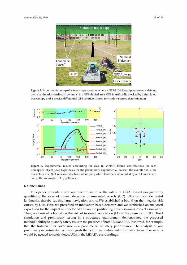
5.2. Preliminary Testing in an Incorrect-Association-Free Environment

Preliminary experimental testing was carried out using data collected in a structured

environment shown in Figure 5. Static simple-shaped landmarks were located at locations sparse

enough to ensure successful outcomes for FE and DA. Because the results presented here were free

of incorrect associations, )( kHMIP was expected to match )|( Kk CAHMIP . This test data was used

to focus on the risk of UO misdetection.

Measurements from carrier phase differential GPS (CPDGPS) as well as LiDAR scanners were

synchronized and recorded. In order to obtain a full 360-degree LiDAR scan, two 180-degree LiDAR

scanners were assembled back-to-back. The LiDAR scanners had a specified 15–80-m range limit, a

0.5-degree angular resolution, a 5-Hz update rate, and a ranging accuracy of 1–5 cm (1 sigma) [42].

The GPS antenna was mounted on top of the front LiDAR. The lever-arm distance between the two

LiDARs was accounted for. The two LiDARs and the GPS antenna were mounted on a rover also

carrying the GPS receiver and data-link. An embedded computer onboard the vehicle recorded all

measurements including the raw GPS data from the reference station transmitted via a wireless

spread-spectrum data-link. Truth trajectory was obtained using a fixed CPDGPS solution.

The upper LHS chart in Figure 6 confirms that this is an incorrect-association-free scenario

because the actual error (thick line) fits within the covariance envelope (thin line) throughout the test.

In addition, the lower LHS graph in Figure 6 shows )( kHMIP -bound contributions for each single-

UO hypothesis. The six )( kHMIP bounds corresponding to UO hypotheses are shown using the

same color code as in Figure 4, and the UO-free hypothesis is the dashed line. The color code is used

on the RHS chart, which also shows the landmark geometry. In the LHS graph, )( kHMIP increases

substantially when accounting for undetected UO (thick black curve), as compared to ignoring their

potential presence (dashed red line). UO occluding landmarks “1” and “2” cause by far the largest increase in )( kHMIP bound. In this SLAM-type implementation where the map is built

incrementally, landmarks observed early in the rover trajectory play a key role throughout the

mission, which explains the method’s sensitivity to potential extraction faults on landmarks “1” and

“2”. In future work, we will try to reduce the )( kHMIP bound using redundant information from

other sensors, from additional landmarks, and from additional landmark features.

5 10 15 20 25 30 35 40 45 5010

-10

10-8

10-6

10-4

10-2

100

Travel Distance (m)

Inte

gri

ty R

isk

P(HMIk)

P(HMIk | H

0)

P(HMIk | H

1)

P(HMIk | H

2)

P(HMIk | H

3)

P(HMIk | H

4)

P(HMIk | H

5)

P(HMIk | H

6)

-30 -20 -10 0 10 20 300

10

20

30

40

50

60

12

3

4

5 6

Time: 29 s

East (m)

No

rth

(m

)

(a) (b)

Sensors 2018, 18, 2740 13 of 17

Figure 5. Experimental setup of a forest-type scenario, where a GPS/LiDAR-equipped rover is driving

by six landmarks (cardboard columns) in a GPS-denied area. GPS is artificially blocked by a simulated

tree canopy and a precise differential GPS solution is used for truth trajectory determination.

Figure 6. Experimental results accounting for UOs (a) P(HMIk)-bound contributions for each

unmapped object (UO) hypothesis for the preliminary experimental dataset: the overall risk is the

thick black line. (b) Color-coded subsets identifying which landmark is occluded by a UO under each

one of the six single-UO hypotheses.

6. Conclusions

This paper presents a new approach to improve the safety of LiDAR-based navigation by

quantifying the risks of missed detection of unwanted objects (UO). UOs can occlude useful

landmarks, thereby causing large navigation errors. We established a bound on the integrity risk

caused by UOs. First, we presented an innovation-based detector, and we established an analytical

expression for the impact of undetected UO on the positioning error assuming correct association.

Then, we derived a bound on the risk of incorrect association (IA) in the presence of UO. Direct

simulation and preliminary testing in a structured environment demonstrated the proposed

method’s ability to quantify safety risks in the presence of both UOs and IAs. It showed, for example,

that the Kalman filter covariance is a poor metric of safety performance. The analysis of our

preliminary experimental results suggests that additional redundant information from other sensors

would be needed to safely detect UOs in the LiDAR’s surroundings.

AGV

Simulated tree canopy

Landmarks

(‘trees’)

Nominal

Trajectory

Laser Scanner

GPS Antenna

90 100 110 120 130 140 150-0.2

0

0.2

Travel Distance (m)

Ea

st (m

)

90 100 110 120 130 140 15010

-10

10-8

10-6

10-4

10-2

100

Travel Distance (m)

Inte

gri

ty R

isk

P(HMIk)

P(HMIk | H

1)

P(HMIk | H

2)

P(HMIk | H

3)

P(HMIk | H

4)

P(HMIk | H

5)

P(HMIk | H

6)

P(HMIk | H

0)

-30 -20 -10 0 10 20 3090

100

110

120

130

140

150

East

No

rth

(a) (b)

Sensors 2018, 18, 2740 15 of 17

Hence, Equation (20). 2

,MDE l is the smallest value of the test statistic NCP that can cause no

detection with probability lower than ,MDE lI . Any error larger than that will be detected with

probability larger than 1-,MDE lI , which is considered safe. Substituting Equation (A4) into (A3),

Equation (A3) becomes

2 2

, , ,( ) ( | )l l l MIN l MDE l MDE lP ND IA P IA y I + (A6)

As described in Section 2, the IA event may be expressed as 2 2

, 0,l MIN l lIA when the “MIN ”

differs from 0. We address the fact that the random variables 2

,MIN l and 2

0,l are correlated using the

exact same steps as in [28]. The derivation in [28] shows that the following event includes lIA :

1

, , , 4T T

MIN l MIN l MIN l l l

− y Y y q q (A7)

where

,MIN ly is defined in Equation (7) and is not zero because of IA (not due to UOs);

,MIN lY is defined in Equation (9);

lq is an ( ) 1l ln m+ vector such that ,~ ( , )l l

l Q l n mN

+q μ I ;

4 the factor four is derived in [28] by solving an eigenvalue problem involving a sum of two

idempotent matrices.

In this work, we distinguish the impacts of the IA and UO. Recall that the CA is the one where

all landmarks that are not occluded by a UO are correctly associated, i.e., where the innovation vector

would be zero mean if the UO was removed. The mean contribution due to IA is accounted for with

,MIN ly on the left-hand side of (A7). In contrast with [28], lq is not zero mean because of the presence

of a UO. Following the eigenvalue solution provided in [28], the maximum impact of UO on the right-

hand-side term is 2

,4 MDE l . After dividing both sides of Equation (A7) by 4, the probability of

occurrence of the event in Equation (A7) is expressed in Equation (19).

References

1. Joerger, M.; Duenas Arana, G.; Spenko, M.; Pervan, B. Landmark Data Selection and Unmapped Obstacle

Detection in Lidar-Based Navigation. In Proceedings of the ION GNSS+, Portland, OR, USA, 25–29

September 2017.

2. U.S. Department of Transportation (DOT) National Highway Traffic Safety Administration (NHTSA).

Available online: https://www.nhtsa.gov/manufacturers/automated-driving-systems (accessed on 18 May

2018).

3. Federal Automated Vehicles Policy—September 2016. Available online:

https://www.transportation.gov/AV/federal-automated-vehicles-policy-september-2016 (accessed on 18

May 2018).

4. RTCA Special Committee 159, Minimum Aviation System Performance Standards for the Local Area

Augmentation System (LAAS). Available online: https://standards.globalspec.com/std/11988/rtca-do-245

(accessed on 18 May 2018).

5. DOT Federal Highway Administration (FHWA), Vehicle Positioning Trade Study for ITS Applications.

Available online: https://rosap.ntl.bts.gov/view/dot/3319/Print (accessed on 18 May 2018).

6. Lee, Y.C. Analysis of Range and Position Comparison Methods as a Means to Provide GPS Integrity in the

User Receiver. In Proceedings of the 42nd Annual Meeting of The Institute of Navigation (1986), Seatle,

WA, USA, 24–26 June 1986.

7. Parkinson, B.W.; Axelrad, P. Autonomous GPS Integrity Monitoring Using the Pseudorange Residual. J.

Inst. Navig. 1988, 35, 255–274.

8. RTCA Special Committee 159, Minimum Operational Performance Standards for Global Positioning

System/Wide Area Augmentation System Airborne Equipment. Available online:

https://standards.globalspec.com/std/1239716/rtca-do-229 (accessed on 18 May 2018).

Sensors 2018, 18, 2740 16 of 17

9. Lu, F.; Milios, E. Globally Consistent Range Scan Alignment for Environment Mapping. Ayton. Robots 1997,

4, 333–349.

10. Röfer, T. Using Histogram Correlation to Create Consistent Laser Scan Maps. IEEE Intell. Robots Syst. 2002,

1, 625–630.

11. Diosi, A.; Kleeman, L. Laser scan matching in polar coordinates with application to SLAM. IEEE Robots

Syst. 2005, 5, 3317–3322.

12. Bengtsson, O.; Baerveldt, A.J. Robot localization based on scan-matching-estimating the covariance matrix

for the IDC algorithm. Robot. Autom. Syst. 2003, 44, 29–40.

13. Rusinkiewicz, S.; Levoy, M. Efficient Variants of the ICP Algorithm. In Proceedings of the Third

International Conference on 3-D Digital Imaging and Modeling, Quebec City, QC, Canada, 28 May–1 June

2001.

14. Bar-Shalom, Y.; Fortmann, T.E.; Cable, P.G. Tracking and Data Association. Math. Sci. Eng. 1988, 179, 918–919.

15. Leonard, J.; Durrant-Whyte, H. Directed Sonar Sensing for Mobile Robot Navigation; Springer: New York, NY,

USA, 1992.

16. Thrun, S. Robotic Mapping: A Survey. In Exploring Artificial Intelligence in the New Millenium; Lakemeyer,

G., Nebel, B., Eds.; Morgan Kaufmann: San Francisco, CA, USA, 2003.

17. Cooper, A.J. A Comparison of Data Association Techniques for Simultaneous Localization and Mapping.

Master’s Thesis, Massachussetts Institute of Technology, Cambrige, MA, USA, 2005.

18. Ruiz, I.T.; Petillot, Y.; Lane, D.M.; Salson, C. Feature Extraction and Data Association for AUV Concurrent

Mapping and Localisation. In Proceedings of the 2001 ICRA. IEEE International Conference on Robotics

and Automation (Cat. No.01CH37164), Seoul, Korea, 21–26 May 2001.

19. Tareen, S.A.K.; Saleem, Z. A comparative analysis of SIFT, SURF, KAZE, AKAZE, ORB, and BRISK. In

Proceedings of the 2018 International Conference on Computing, Mathematics and Engineering

Technologies (iCoMET), Sukkur, Pakistan, 3–4 March 2018.

20. Dissanayake, G.; Newman, P.; Clark, S.; Durrant-Whyte, H.; Csorba, M. A Solution to the Simultaneous

Localization and Map Building (SLAM) Problem. IEEE Trans. Robot. Autom. 2001, 17, 229–241.

21. Feng, Y.; Schlichting, A.; Brenner, C. 3D Feature Point Extraction from LiDAR Data Using a Neural

Network. In Proceedings of the International Archives of the Photogrammetry, Remote Sensing and Spatial

Information Sciences, Prague, Cezch, 12–19 July 2016.

22. Li, Y.; Olson, E.B. A General Purpose Feature Extractor for Light Detection and Ranging Data. Sensors 2010,

10, 10356–10375.

23. Kim, J.; Kang, H. A New 3D Object Pose Detection Method Using LIDAR Shape Set. Sensors 2018, 18, 882.

24. Bar-Shalom, Y.; Daum, F.; Huang, J. The Probabilistic Data Association Filter. IEEE Control Syst. Mag. 2009,

29, 82–100.

25. Areta, J.; Bar-Shalom, Y.; Rothrock, R. Misassociation Probability in M2TA and T2TA. J. Adv. Inf. Fusion

2007, 2, 113–127.

26. Joerger, M.; Jamoom, M.; Spenko, M.; Pervan, B. Integrity of Laser-Based Feature Extraction and Data

Association. In Proceedings of the 2016 IEEE/ION Position, Location and Navigation Symposium (PLANS),

Savannah, GA, USA, 11–14 April 2016.

27. Joerger, M.; Pervan, B. Continuity Risk of Feature Extraction for Laser-Based Navigation. In Proceedings

of the 2017 International Technical Meeting of The Institute of Navigation, Monterey, CA, USA, 30 January–2 February 2017.

28. Joerger, M.; Pervan, B. Quantifying Safety of Laser-Based Navigation. IEEE Trans. Aerosp. Electron. Syst.

2018, doi:10.1109/TAES.2018.2850381.

29. Kim, C.; Lee, Y.; Park J.; Lee, J. Diminishing unwanted objects based on object detection using deep learning

and image inpainting. In Proceedings of the 2018 International Workshop on Advanced Image Technology

(IWAIT), Chiang Mai, Thailand, 7–9 January 2018.

30. Asvadi, A.; Premebida, C.; Peixoto, P.; Nunes, U. 3D Lidar-based static and moving obstacle detection in

driving environments: An approach based on voxels and multi-region ground planes. Robot. Autom. Syst.

2016, 83, 299–311.

31. DeCleene, B. Defining Pseudorange Integrity—Overbounding. In Proceedings of the 13th International

Technical Meeting of the Satellite Division of The Institute of Navigation (ION GPS 2000), Salt Lake City,

UT, USA, 19–22 September 2000.

Sensors 2018, 18, 2740 17 of 17

32. Rife, J.; Pullen, S.; Enge, P.; Pervan, B. Paired Overbounding for Nonideal LAAS and WAAS Error

Distributions. IEEE Trans. Aerosp. Electron. Syst. 2006, 42, 1386–1395.

33. Arana, G.D.; Joerger, M.; Spenko, M. Minimizing Integrity Risk via Landmark Selection in Mobile Robot

Localization. IEEE Trans. Robot. 2017, in press.

34. Tanil, C.; Khanafseh, S.; Joerger, M.; Pervan, B. An INS Monitor to Detect GNSS Spoofers Capable of

Tracking Vehicle Position. IEEE Trans. Aerosp. Electron. Syst. 2018, 54, 131–143.

35. Tanil, C.; Joerger, M.; Khanafseh, S.; Pervan, B. A Sequential Integrity Monitoring for Kalman Filter

Innovations-Based Detectors. In Proceedings of the ION GNSS+, Miami, FL, USA, 24–28 September 2018.

36. Joerger, M.; Chan, F.-C.; Pervan, B. Solution Separation Versus Residual-Based RAIM. J. Inst. Navig. 2014,

64, 273–291.

37. Joerger, M.; Pervan, B. Kalman Filter-Based Integrity Monitoring Against Sensor Faults. J. Guid. Control

Dyn. 2013, 36, 349–361.

38. Pullen, S.; Lee, J.; Luo, M.; Pervan, B.; Chan, F.-C.; Gratton, L. Ephemeris Protection Level Equations and

Monitor Algorithms for GBAS. In Proceedings of the ION GPS 2001, Salt Lake City, UT, USA, 11–14

September 2001.

39. Pullen, S. Augmented GNSS: Fundamentals and Keys to Integrity and Continuity. In Proceedings of the

ION GNSS 2011, Portland, OR, USA, 19–23 September 2011.

40. Joerger, M.; Pervan, B. Measurement-Level Integration of Carrier-Phase GPS and Laser-Scanner for

Outdoor Ground Vehicle Navigation. J. Dyn. Syst. Meas. Control 2009, 131, 021004.

41. Joerger, M. Carrier Phase GPS Augmentation Using Laser Scanners and Using Low Earth Orbiting

Satellites. Ph.D. Dissertation, Illinois Institute of Technology, Chicago, IL, USA, 2009.

42. Ye, C.; Borenstein, J. Characterization of a 2-D Laser Scanner for Mobile Robot Obstacle Negotiation. In

Proceedings of the 2002 IEEE International Conference on Robotics and Automation (Cat. No.02CH37292),

Washington, DC, USA, 11–15 May 2002.

© 2018 by the authors. Licensee MDPI, Basel, Switzerland. This article is an open access

article distributed under the terms and conditions of the Creative Commons Attribution

(CC BY) license (http://creativecommons.org/licenses/by/4.0/).