a new approach to the construction of optimal designsneilsloane.com/doc/me175.pdf · r.h. hardin,...

Journal of Statistical Planning and Inference 37 (1993) 339-369

North-Holland

339

A new approach to the construction of optimal designs

R.H. Hardin and N.J.A. Sloane

AT&T Bell Laboratories, Murray Hill, NJ, USA

Received 15 February 1992; revised manuscript received 20 October 1992

Abstract

By combining a modified version of Hooke and Jeeves’ pattern search with exact or Monte Carlo moment

calculations, it is possible to find I-, D- and A-optimal (or nearly optimal) designs for a wide range of

response-surface problems. The algorithm routinely handles problems involving the minimization of

functions of 1000 variables, and so for example can construct designs for a full quadratic response-surface

depending on 12 continuous process variables. The algorithm handles continuous or discrete variables,

linear equality or inequality constraints, and a response surface that is any low degree polynomial. The

design may be required to include a specified set of points, so a sequence of designs can be obtained, each

optimal given that the earlier runs have been made. The modeling region need not coincide with the

measurement region. The algorithm has been implemented in a program called gosset, which has been used

to compute extensive tables of designs. Many of these are more efficient than the best designs previously known.

AMS Subject Classification: Primary 62K05

Key words and phrases: A-optimal, D-optimal, I-optimal, minimal designs, mixture designs, rotatable

designs, quadratic designs

1. Introduction

This paper presents a new algorithm for constructing experimental designs. The

algorithm, described in Section 3, has the following features.

(a) The variables may be discrete or continuous (or both - none of these choices

are mutually exclusive), discrete variables may be numeric or symbolic, continuous

variables may range over a cube or a ball, and the variables may be required to satisfy

linear equality or inequality constraints (so mixtures and constrained mixtures can be

handled).

(b) The model to be fitted may be any low degree polynomial (for example

a quadratic response-surface).

Correspondence to: N.J.A. Sloane, A.T.&T. Bell Laboratories, Murray Hill, NJ 07974, USA.

037%3758/93/%06.00 @,? 1993 ~ Elsevier Science Publishers B.V. All rights reserved

340 R.H. Hardin, N.J.A. Sloane/The construction of optimal designs

(c) The number of runs is specified by the user (so minimal designs present no

difficulty).

(d) The design may be required to include a specified set of points (so a sequence of

designs can be found, each of which is optimal given that the earlier measurements

have been made).

(e) The region where the model is to be fitted need not be the same as the region

where measurements are to be made. (So for example designs can be optimized for

modeling over a continuous region even if the measurements are constrained to

a disvtrete set. Designs for extrapolation can be obtained in a similar way).

(f) The algorithm is capable of minimizing any optimality criterion that is differen-

tiable or can be approximated by a differentiable function. We have focused on four

such criteria, I-, A-, D- and E-optimality, with a distinct preference for the first, which

minimizes the average prediction variance (see Section 2). The I-optimality criterion

requires knowledge of the moments of the design region, and the algorithm finds these

moments either from the exact formulae or by Monte Carlo estimation.

(g) The user has control over how much effort is expended by the algorithm, and

can if desired monitor the progress of the search. It is not necessary to specify initial

points for the search.

(h) The algorithm can be used in situations in which the errors, rather than being

independent, have a known correlation matrix.

The algorithm appears to be powerful enough to find optimal or nearly optimal

designs involving as many as 1000 continuous variables, for example a full quadratic

response-surface design depending on 12 process variables. Its effectiveness decreases

as the number of discrete variables increases. However, the algorithm has-found

D-optimal main-effect designs involving 20 2-level factors (i.e., with 420 discrete

variables).

No individual ingredient of our algorithm is new. But although computers have

been used by many people to construct experimental designs (surveys of such work

can be found for example in Box and Draper, 1987, Chap. 15; Cook and Nachtsheim,

1980; Dodge et al., 1988; Lucas, 1976; Myers et al., 1989; Nachtsheim, 1987; St. John

and Draper, 1975; Steinberg and Hunter, 1984; Yonchev, 1988) we believe that no

algorithm comparable to ours is presently available.

Implementation

We have implemented the algorithm in the C language in a program called gosset.

A built-in parser permits a very flexible input. A brief description is given in Section 4,

and further details can be found in the users’ manual, Hardin and Sloane (1992).

The program is named after the amateur mathematician Thorold Gosset

(1869-1962) who was one of the first to study polytopes in six, seven and eight

dimensions (Coxeter, 1973, p. 164) and his contemporary, the statistician William

Seally Gosset (1876-1937) who was one of the first to use statistical methods in the

R.H. Hardin, N.J.A. Sloane/The construction of optimal designs 341

planning and interpretation of agricultural experiments (Pearson and Wishart, 1942).

Although from our geometric viewpoint their work is related, we do not know if the

paths of Thorold (Cambridge, London, lawyer), and William Seally (Oxford, Dublin,

brewer) ever crossed.

Applications

So far there have been two main uses for gosset.

(i) We have attempted to construct optimal (especially Z-optimal) designs

for a number of ‘classical’ situations, for example linear, quadratic or cubic response-

surface designs with k continuous variables in a cube or ball with n runs, over

quite a large range of values of k and n, typically 1 d k d 12 and IZ ranging from

the minimal value to 6 (or more) greater than the minimal value. We have also

computed designs for similar models and regions in which the variables are discrete.

An extensive library of these designs is now built into gosset. Our work on these

‘classical’ problems can be regarded as an attempt to provide optimal ‘exact’ designs

with small numbers of runs to complement the ‘asymptotic’ designs of Kiefer et al.

(Farrell, Kiefer and Walbran, 1967; Galil, 1985; Galil and Kiefer, 1977a, b, 1979,

1980a, b, c, 1982a, b).

As we shall see in Section 5, some of these designs overlap with and improve on

designs already available in the literature. Other designs we have found will be

published elsewhere (see Hardin and Sloane, 1992a, b, c, d).

We have also used this collection of designs as data for theoretical investigations.

Two results are worth mentioning here.

(a) There is a simple lower bound on the average variance of an I-optimal design

for quadratic models with n measurements in a k-dimensional ball (see

equation (13) below). A number of interesting designs meet the bound. There

is a similar bound for D-optimal designs.

(b) It is known that for large numbers of runs D- and G-optimal designs are

equivalent (Kiefer and Wolfowitz, 1960). The results of Section 5 show that

I-optimal designs are strictly different. For example, Z-optimal designs make

more measurements at the center of the region and fewer at the boundary.

For quadratic models in a k-dimensional ball, k large, an I-optimal design

makes about 4/k’ of the measurements at the center of the sphere, compared

with about 2/k’ for D- and G-optimal designs. I-optimality also appears to be

a more strict condition than D-optimality. In situations where the criteria

produce similar designs (such as certain linear designs, see Section 5.3), we

commonly find that although I-optimal designs are D-optimal, the converse

is not necessarily true.

(ii) We have constructed designs for a number of industrial applications, for

instance problems involving continuous and discrete variables simultaneously, with

linear constraints on the variables (see Section 5.4).


We must emphasize that the theoretical justification for our designs (see Section 2)

depends strongly on the validity of the particular model being used. We are assuming

that the investigator has carried out some exploratory investigations (for example

a screening design) and has identified a region where it is plausible to describe the

response by a low degree polynomial. (Of course the design points when the initial

measurements have been made can be incorporated by our program in the next design

- see Section 4.)

This work began in 1990 when a statistician in Seattle, David H. Doehlert, wrote to

one of us asking if we could construct designs for a full quadratic response-surface

depending on k variables in a sphere, where k is between 3 and 14, and in which the

number of runs is minimal or close to minimal. We had been using the pattern search

algorithm in studying the Tammes problem of placing M points on a k-dimensional

sphere so they are well-separated (Hardin et al., 1993) and we found that a similar

approach could be used for constructing designs.

2. Choice of optimality criterion

Extensive discussions of the relative merits of A-, D-, E-, G- and I-optimality and

of the dangers of relying on any single numerical criterion have appeared in

the literature (see for example Box and Draper, 1987, 1971; Giovannitti-Jensen

and Myers, 1989; Kiefer, 1985; St. John and Draper, 1975), and our treatment will

be brief.

Suppose for concreteness that we wish to construct a design for a full quadratic

response-surface model

_Y=PO+iil Pixi+iil Piixf+‘il i Bijxixj+G

i=l j=i+l (1)

where there are k variables x1,..., xk, P=+ (k+ 1) (k +2) unknown coefficients p, and

the errors E are independent with mean 0 and variance c?. Let the design consist of

n > p points

[xjl,...,xjk] for 1 <j<n, (2)

chosen from a certain region of measurement (or operability) 0. Let X be the n x p expanded design matrix, containing one row

for each design point x = [x1,. . ., xk], and let

M,,1 X’X n


denote the matrix of moments of the design measure (the prime indicates matrix

transposition). The prediction variance at an arbitrary point x is

var j(x) = gf (x) M; ‘f(x).

We define an I-optimal design (following Box and Draper, 1963,1987; and others) to

be one which minimizes the normalized average or integrated prediction variance

I=$ s var P (4 dp (4, R

where R is the region of interest (or modeling region), and p is uniform measure on

R with total measure 1. This integral simplifies (cf. Box and Draper, 1987, p. 341) to

give

I = trace {MM, ’ }, (4)

where

M = s

f(x)‘f(x) d/M R

(5)

is the moment matrix of the region of interest.

In contrast, A-, D-, E- and G-optimal designs are those which minimize

A=trace M;‘, (6)

D = { det M,} - ‘lp,

E = maximal eigenvalue of M; ‘,

(7)

(8)

G = maximal value of varf(x), x E R, (9)

respectively. We shall refer to the quantities defined in (4), (6)-(9) as the I-, A-, etc.,

values of the design. As the number of runs n-00, these quantities approach limits

I,, A,, etc., and the I-, A-, etc. efJiciencies of the design are given by

1, A, D, E, G, --- TA’D’ E’ G (10)

(cf. Atwood, 1969; Lucas, 1976).

We are most interested in minimizing the prediction variance, var?(x), for

x E R, which suggests the use of I-, or G-optimality. On the other hand our algo-

rithm requires that the criterion be differentiable, which holds for A-, D- and I- but

not G-optimality. (We obtain E-optimality as a limit.) Furthermore we wish to be able

to construct designs for which the measurement region 0 and modeling region R are

distinct, which also picks out the I- or G-criteria (since the A-, D- and E-criteria do not

involve R). We have therefore chosen I-optimality as our primary criterion. However,

the implementation of the algorithm allows the user to search for any of I-, A-, D- or

E-optimal designs.

344 R.H. Hardin, N.J.A. Sloane/ The construction of optimal designs

It is worth mentioning that the Z-value (equation (4)) is a dimensionless quantity.

Also, provided the model has the property that if it contains one monomial of degree

d then it contains all possible monomials of degree d d, then the Z-value is unchanged

if the variables are resealed or if an orthogonal transformation is applied to the

variables. In contrast the A- and E-values of a design depend on the particular choice

of coordinate axes used, a property which seems unsatisfactory. In the present paper

we shall concentrate on I- and D-efficiencies. For the ball or cube it is not difficult to

determine I, and D, exactly. In other cases we determined them empirically, by

estimating the limiting values of I and D as the number of runs increases. We

attempted to calculate I, and D, to at least three decimal places of accuracy.

However, inaccuracies in I, and D, are not too significant, because they do not

change the relative efficiencies of comparable designs. Note that a design is I- (or D-) optimal if it has the highest I- (or D-) efficiency for a given number of runs, and so

a design can be optimal without being 100% efficient.

To guard against the dangers of using any single number as a design criterion, we

have plotted variance dispersion graphs (Giovannitti-Jensen and Myers, 1989; Vining,

1990) for our designs; some examples will be found in Hardin and Sloane (1992a).

These graphs show how the prediction variance varf^(x) varies over the region of

interest, and also give the G-value of the design.

We conclude this section by briefly mentioning some earlier papers that look for

Z-optimal designs.

Studden (1977) gives a method for constructing approximations to Z-optimal

designs for l-dimensional problems.

Haines (1987), Myer and Nachtsheim (1988), Crary (1991) and Snow and Crary

(1991) all use simulated annealing to search for Z-optimal designs. This approach

seems to be restricted to low dimensions and small numbers of design points, and

furthermore is less successful at finding optimal designs than our approach. For

example, gosset finds slightly different designs in two of the four cases shown in

Figure 1 of Crary (1991). Meyer and Nachtsheim (1988) give several quite small

examples where simulated annealing was unable to find the best designs known. One

of these, a 17-run four-dimensional example, is described in Section 5.2 below.

Crary’s (1991) program, Z-OPT, like ours, allows the measurement and modeling

regions to be distinct. Z-OPT has a feature that gosset does not have at present,

namely the ability to specify relative weights for points in the modeling region.

3. The algorithm

For a given model (such as (1)) involving k variables and p unknown coefficients,

a design consists of n points (2) (not necessarily distinct) in the region 0. Let x be

a vector specifying the coordinates of all the design points. We wish to choose the

design vector x so as to minimize a certain differentiable function F(x). For Z-optimal


designs, F is the normalized average prediction variance I = trace MM, I, where M is

the moment matrix of the region R (see (4), (5)), while for A- or D-optimality F is trace

M,’ or {det Mx)-l’p (see (6), (7)). We let g(x) d enote the gradient VF (x), normalized

to have length &.

The regions 0 and R can be quite complicated. The present implementation (see

Section 4) permits 0 and R to be a product of cubes, balls and finite sets, possibly

intersected by hyperplanes and half-spaces. This includes simplices, of course, since

these are intersections of cubes and hyperplanes.

If there are no equality constraints in the problem then the design vector x is simply

a concatenation of the individual points (2) of the design. When equality constraints

are present we choose new, internal, variables to parametrize the space 0, and then

x is a concatenation of the coordinates of the internal variables.

If the region 0 is a simple connected space such as a ball, our basic strategy is to

minimize F using a modified version of the Hooke and Jeeves (1961) pattern search.

An excellent description is given by Beightler et al. (1979), and our discussion here will

be brief. We have modified the algorithm to make use of the gradient of F. Roughly

speaking, pattern search minimizes F by accelerating down the gradient, and setting

the velocity to zero whenever the function does not improve. The velocity increases as

long as improvements continue.

We begin with an initial design vector X=X(‘), with velocity u’~‘=O. This initial

design may be obtained by choosing n random points from 0, although in the

implementation the user has the option of specifying x (‘) himself. We attempt to define

the next vector by

#+ 1) =X(i)+v(i+ 1)

where the velocity vector u(~“) is given by

(11)

v(i+ 1) =a(i)--s8(x(i)), (12)

for i 30, where s is the current step size. If F(x(‘+ ‘)) < F(x(‘)) the step is a success, we

accept this value for x@+l), and repeat the iteration with s multiplied by 1.04.

Otherwise we set uCi) =0 and try (11) and (12) again. If there is still no reduction in F, we divide the step size by 2, and if it is larger than some small accuracy limit, try (11)

and (12) again. Otherwise we terminate this attempt, pick another starting design

x(O), and repeat the whole procedure. Any particular sequence F (.d”‘), F (x”‘), F (d2)), . . . (a decreasing, hence bounded, sequence of positive numbers) is terminated

either when the step size is less than some small accuracy limit, or (very rarely) when

the number of steps exceeds a specified limit. After a specified number of attempts the

algorithm terminates, returning the best and the most recent second-best designs

found.

Equations (11) and (12) must be modified when the design vector x(“) involves points

near the boundary of 0 (either the natural boundary, for instance when 0 is a ball,

cube or simplex, or a boundary imposed by a constraint on the variables). When this


happens, the components of the gradient vector crossing the boundary are simply

zeroed before normalization, and if any point in x(“) nevertheless moves outside the

boundary we move it to the closest point on the boundary.

Incidentally, in the implementation the gradient is calculated from the exact

formula for VF, rather than by numerical differentiation of F. We have found this method very robust and efficient, typically minimizing a func-

tion of N variables in N steps.

The above procedure is used when all or most of the variables in the design are

continuous. When many discrete variables are present we use a collection of heuristic

algorithms (which do however work most of the time).

Suppose for concreteness that there are k=6 variables, the first four of which

are continuous and the last two are discrete variables. Let the n points of the

design be

a=ar ... &j , &=bl... bs, . . . , c=cl ‘.. c6,

so that the design vector is x=ab ... c.

We first discuss the question of choosing the discrete coordinates

%, a6, b5, 66, . .’ , c5, c6 of the initial design vector x (‘I For this we use one (or more) of .

three strategies: (i) run sequentially through all possibilities in some fixed order,

running through them all once before repeating any; (ii) choose them at random from

the set of all discrete possibilities; (iii) choose them at random from the underlying

continuous space. If constraints are present, in all three cases only points satisfying the

constraints are used. Strategies (i) and (ii) are reasonable when the number of

combinations of discrete variables is not much larger than the number of design

points, otherwise (iii) appears to be more successful. In the implementation the user

can specify the strategy to be used, or accept the default strategy (which depends on

the type of problem).

Second, in the optimization step, we optimize (using the method described earlier

in this section) either just the continuous components of x, keeping the dis-

crete components fixed, or all components, treating the discrete components as

continuous.

If the latter strategy is adopted, a final step is needed to convert the discrete

components (u5, a6, etc.) back to their permitted discrete values. For this discretization

step we again use one of three methods, replacing each continuous component by: the

closest discrete value, whichever of the two closest discrete values gives the smallest

value of F, or whichever of the discrete values gives the smallest value of F. We have

found the second of the three methods works best, the third being too slow. All three

methods go through the components of x in order, making a decision and not

changing it again. These are ‘greedy’ techniques, and do not try to avoid getting

trapped at local minima. Again the user can, if desired, control which method is used.

There is a complication to the discretization step, however, for the resulting vector

x may now violate some constraints involving the discrete variables. If so, we attempt


to adjust both the continuous and discrete components of x to correct this. Again

we use one of three methods, the most successful of which is the following. We

first find the closest vector x’ (say) to x that satisfies all the constraints, treating

the discrete components as continuous again. Then we generate a number of

random legal vectors that satisfy all the constraints and have continuous or

discrete components as appropriate, and pick the ten of these that are closest to x’.

In computing their distance to x’, we only consider components that are involved

in constraints (the others being irrelevant here). From these ten vectors we select

the one that minimizes F (again using only the components that are involved

in constraints). This vector is properly discrete and satisfies all the constraints. A

final optimization is then made with respect to the continuous variables only.

The modeling region, R, enters the algorithm only through the moment matrix

M (see (5)). For simple regions (balls, cubes, discrete sets) we use the exact moment

matrix (cf. Box and Draper, 1959, 1963) otherwise we estimate them by a Monte

Carlo method. In the present implementation the most general region R is a subset of

a region SZ(say) which is a product of balls, cubes and discrete sets. The algorithm

generates random points with a uniform distribution over 52. If the point satisfies all

the constraints it is accepted and its contributions towards the entries of M are

recorded. The user has the option of controlling the number of Monte Carlo samples

used.

The more samples used, the more accurate is the matrix. It is usually not too serious

for nontheoretical applications if the matrix is inaccurate - this corresponds to

a slight change in shape of the region of modeling.

Two features of the algorithm are worth mentioning. If the user discovers that

greater accuracy in the moment matrix is called for, further Monte Carlo trials can be

run, and the results will be automatically combined with the previous estimates.

Second, the algorithm checks to see if the region R is invariant under changing the

sign of any coordinates or under permutation of the coordinates and, if so, automati-

cally makes M invariant under the same symmetries.

4. Implementation: the program gosset

The algorithm has been implemented in the C language in a program called gosset.

The program takes about 10,000 lines of code, runs on a variety of UNIXQbased

machines, and is distributed in conjunction with the S statistical programming

language (Becker et al., 1988). Only a brief description is given here; full details can be

found in the manual of Hardin and Sloane (1992).

There are three basic steps in using gosset: specifying the design, calculating the

moment matrix, and searching for the optimal design.

Step 1. Design speccjication. The design is specified by a series of numbered lines,

somewhat like a BASIC program. Variables are specified by lines such as

348 R.H. Hardin, N.J.A. Sloane1 The construction of optimal designs

10 range a b c 90 120

20 sphere Temp Zinc Water center 300 20 4 radius .5

30 discrete KEV 70 90 100

which indicate that a, b, c are continuous variables ranging from 90 to 120; Temp,

Zinc and Water belong to a ball centered at [300, 20, 503 of radius 0.5, and KE V is a quantitative discrete variable with values 70, 90, 100. Any number of such lines may

appear.

To allow a more flexible input format, the program includes its own parser.

(Programs such as YACC and LEX (see Hume and McIlroy, 1990) have made people

forget how easy it is to write a parser starting from scratch.)

Lines lo-30 above are contravariant specifications of scaling, but it is often more

convenient to use a covariant form. Line 20 for example could equally well be written

20 sphere 2* (Temp - 300) 2* (Zinc - 20) 2* (Water -4)

since the default radius is 1 and the default center is the origin. Gosset accepts either

form, or any combination of them.

Unprimed variables describe the region of measurement (0) and matching primed

variables describe the region of modeling (R). The absence of primed variables

indicates that 0 and R coincide. For example

10 discrete a b c -1 1

20 range a’ b’ c’ -1 1

specifies that a, b, c are 2-level discrete variables taking the values -1 and 1, while the

model is to be fitted over the whole cube C-1, 11”. If line 20 is omitted, the model

would be fitted just on the finite set { -1, l}” where the measurements are to be made.

In this example the numbers -1 and 1 could be omitted, because by default all

variables have limits -1 and 1, and discrete variables are 2-valued.

Constraints (which must be linear) are expressed by lines such as

50 constraint x + 2*y + 3*z = 1

60 constraint A<B B+0.4<C

The specification use forces a given point to appear in the design (for example, runs

made in an earlier experiment, the results of which we do not want to lose). The

program will then search for the best design that includes these points. For example

70 use x= .9 y= .3 material =“plastic”

Inequality constraints may be violated by use points. It may be one of these that

suggested the wisdom of the constraint! (However, because the program handles

equality constraints by eliminating variables, use points must satisfy all equality

constraints.)


The model is specified symbolically, by an expression such as

80 model (1 + a + b +cf2-c-2

which specifies that the model (see equation (1) above) contains the terms 1, a, b, c, a’,

b2, ab, ac, bc, but not c ‘. In the model specification, + means ‘add to the list’, - means

‘take away if it exists’, and multiplication means ‘form all products and keep one

representative of each type of term’. This is similar to the way models are specified in

the S language (Chambers and Hastie, 1991).

Once the design has been specified by a ‘program’ in this way, the program is

compiled by the command

compile

At this point gosset chooses new, internal, variables to parametrize the spaces R and

0, eliminating each equality constraint by dropping a variable, whose range is then

expressed by a pair of inequalities, eliminating clearly redundant or unnecessary

inequalities, and scaling the internal variables so they are in the range -1 to 1.

Step 2. Moment calculation. The second step is to find the moment matrix M (see

previous section) by Monte Carlo estimation with a command such as

moments time = 300 n = 1 O-6

which would sample until either 300 seconds have elapsed or lo6 samples have been

taken. If this is a problem where the program can determine M exactly, the effect will

be as if the user had said

moments n = 0

and the exact moments will be used. The moments command makes a header file

moments.h which is used by the search programs.

Step 3. Searching for an optimal design. The third step is to search for an optimal

design, using a command such as

design type= I runs=24 n =200

This would instruct the program to search for an Z-optimal design with 24 runs, taking

200 random designs, optimizing each of them (using the techniques described in

Section 3), and choosing the best.

The design command has many options. For example, type= I (or D, or A)

searches for an I- (or D- or A-) optimal design. Extra = 3 searches for a design with

three more runs than a minimal design would contain (and relieves the user of the

necessity of counting the terms in the model!). Start =v.l6.old begins the search at

a previous design. Tiny = 1 .Oe - 5, steps = 500, time = 300 set limits to the minimal

step size, the number of steps in the search, and the search time. Processors = 7, on

a multiprocessor machine, would run seven searches in parallel (with of course

a dramatic increase in speed). In the design command, the user can, if desired, control


the search algorithm by the program = option. Program = r means choose a random

start, v minimizes I by changing the continuous variables while keeping the discrete

variables fixed, d is similar but maximizes det M,, vc minimizes I by changing all

variables, treating discrete variables as if they were continuous, and so on.

These symbols can be combined using various operators: + means choose the

best of the left and right sides, A means iterate the left side the number of times

indicated by the right side, and * is a ‘pipe’ command which passes a design on to

the next process.

For example

design program=(r*v)^50+Iib

means generate 50 random starts, optimize each, take the best, and compare with the

best design found in the library.

If the program =option is not used, gosset uses various default programs, for

example program=r * v if there are no discrete variables.

Gosset automatically builds up a library of designs for each problem as it proceeds,

and, as mentioned in Section 5, contains a very extensive built-in library of designs for

the ball, cube, etc.

Gosset does many things simultaneously ~ reads input from the terminal, spins

off jobs to run the Monte Carlo moment calculation, to compute the Z-value

of a design, etc., and also checks from time to time to see if these jobs are finished.

Several difficulties had to be overcome in order to do this in a portable and con-

venient way.

For example, one cannot directly use the UNIX wait system call to see if a job is

finished without being blocked (put to sleep until a termination) if the job is still

unfinished. Of course this would prevent gosset from responding to the terminal. So

every wait system call in gosset is preceded by spinning off a dummy job that does

nothing. Then the wait is sure to complete quickly, because the dummy job terminates

quickly, and if the job we are really interested in is finished we will be told about that

too.

However, some systems always report completed jobs in the reverse order, report-

ing the most recent jobs first. So gosset runs a test when it starts up, and if it discovers

that jobs are reported in the reverse order, makes the dummy jobs sleep for one second

(instead of doing nothing), so they are certain to be reported after other completed

jobs.

Gosset also contains its own ‘input daemon’ to make it possible to read input

without halting the main program. The input daemon program simply waits

until input lines appear, and then writes them to a disk file. The main program does

not read input directly (this would halt the main program if no input were present),

but checks occasionally to see if the disk file has grown, and if so, reads the last

line there.

R.H. Hat-din, N.J.A. Sloane/The construction of optimal designs 351

These features make it possible for a user to monitor the progress of the moments

or design programs, using watch, status or kill commands, to inspect the best design

found so far, or to perform other tasks.

When the design program finishes, the interp command prints out the best design

found, translating from the internal to the original variables. The commands iv, av

and dv respectively calculate the I-, A- and D-values of a design. The program

automatically maintains a library of the best designs found.

Example. The following is an edited transcript of a session in which gosset was used

to search for an I-optimal design with three continuous variables x, y, z, each between

0 and 1, for a full quadratic response surface, with 14 runs (a minimal design would use

10 runs), taking the best of 25 attempts.

10 range xyzO1

20 model (1 +x+y+z)^ 2

compile . . .

moments n = 1 O-6 . . .

design type=1 runs=14 n=25 . . .

interp

0.~000

0.0000

0.0000

0.1707

0.1707

0.4742

0.4742

0.4742

0.6630

0.6630

1 .oooo

1 .oooo

1 .oooo

1 .oooo

iv

0.4065171

Y Z

0.0000 0.0000

0.5000 0.5000

1 .oooo 1 .oooo

0.0000 1 .oooo

1 .oooo 0.0000

0.5000 0.5000

0.5000 0.5000

0.5000 0.5000

0.0000 0.0000

1 .oooo 1 .oooo

0.0000 0.5712

0.4288 1 .oooo

0.5712 0.0000

1 .oooo 0.4288

Note that this design is symmetric in y and z but not x, and that a point close to the

center of the cube appears three times in the design. This is one of many situations in

which a probably optimal design could have been obtained from the built-in library.


We have printed the design rounded to four decimal places, but this is also under

the user’s control. This facility makes it possible to investigate the dependence of

the I-value on the precision of the design points. One could for example print the

design with only two decimal places of accuracy, and recalculate the Z-value. (In

this particular example the I-value increases only by about 0.000004.)

Further examples are given in the following section and in Hardin and

Sloane (1992a, b, c, d). The running time of the program, when searching for a

minimal quadratic design in the k-dimensional ball, grows roughly as k6.

We have recently extended the program by adding the ability to construct designs

for situations in which the errors (in equation (l), for example), rather

independent, have a known correlation matrix. We omit the details.

5. Examples

than being

For over a year we have been running gosset to produce extensive tables of

conjecturally optimal (or nearly optimal) designs for a variety of classical problems.

Once found, these designs are incorporated into gosset’s built-in library. The families

we have focused on are I-optimal designs for linear, quadratic or third-order models,

in the ball or cube, with continuous or discrete (2- or 3-level) variables. Many

D-optimal designs have also been computed.

At the present time the library includes third-order designs for the ball and cube

with 4-20 runs (in 1 dimension), lo-30 runs (in 2 dimensions), 20-30 runs (in

3 dimensions), and 3540 runs (in 4 dimensions), all using continuous variables, as

well as third-order designs for the ball in some higher dimensions. Figure 1 shows the

conjecturally Z-optimal design with 12 runs in two dimensions.

0 0

Fig. 1. Conjecturally I-optimal 12-run design for cubic regression in square.


Table 1

Quadratic response surface designs in gosset library (entry gives number

of runs)

Variables Ball Cube

k (continuous) (continuous)

1 3-30 3-30

2 6-21 6-40

3 10-33 10-30

4 15-28 15-22

5 21-33 21-29

6 28-39 28-36

1 36-54 36-44

8 45-70 45-53

9 55-62 55-63

10 66-74 66-74

11 78-86 78-86

12 91-99 91-98

13 105S113 105-113

14 12OG128 120-128

Discrete Discrete

(k 1) (0, + 1)

2-6 3-7

4-8 6-10

7-11 10-14

11-15 15-19

16-20 21-25

22-26 28-32

29-33 36-40

37-41 45-49

46-50 55-59

56-60 66-70

67-71 78-82

79-83 91-95

These designs are very much smaller than the third-order designs available up to

now (compare Bagchi, 1986; Huda, 1982, 1983; and the references given there). For

example the smallest four-dimensional design presented in these papers has 60 runs.

The parameters of the quadratic designs are shown in Table 1. The columns headed

‘ball’ and ‘cube' refer to designs for the full quadratic model fro +C piXi+CC,,,BijXiXj,

in which the variables may range continuously over a k-dimensional ball or cube, while in

the last column the variables are restricted to points with coordinates -1, 0, +l. For these

three columns the modeling region is the continuous k-dimensional ball or cube. The

column headed ‘Discrete (fl)’ refers to interaction designs, in which the variables are

restricted to points with coordinates f 1, the squared terms PiiX’ (i= 1,. . . , k) are omitted

from the model, and the modeling region is the same discrete set as the measurement

region.

The designs mentioned in the table are usually the best of at least 1000 attempts. Some

of these designs (and the reasons for believing they are close to optimal) are briefly

discussed in the following subsections.

We have made similar, although less extensive, tables of conjecturally D-optimal

quadratic designs, some of which are mentioned in Section 5.2.

As to linear designs, at present the library contains conjecturally I- and D-optimal

designs with k+ 1 runs for k variables taking values f 1, for k= 1,2,. . . ,20,23, 27, 31, . . . ,47. For k= 3 (mod 4) these are Plackett-Burman-Rao designs, while the

others are discussed in Section 5.3.

We have also used gosset to construct other classes of designs: mixture designs

(cf. Cornell, 1990; Vuchkov et al., 1981) block designs, and designs which are intended for

use in circumstances when one of the measurements may be lost.


5.1. Quadratic designs in the ball

Study of the extensive collection of quadratic designs referred to in Table 1 has led

us to make a number of observations about the properties of optimal designs in the

ball.

Let s(k, n) (resp. 9(k, n)) denote any Z-optimal (resp. D-optimal) design for a full

quadratic model using n runs in a k-dimensional ball, for k= 1,2,. . . , and

n >/t (k+ l)(k+2).

We begin with the observation that there appears to be a unique design 9(3, 14) (apart

from orthogonal transformations), which consists of three copies of a point distant

0.003622 from the center of the ball and eleven points on the surface of the

ball. The precise design is given in Hardin and Sloane (1992~). However, restricting

S(3, 14) to points at the center and on the surface of the ball incurs a loss of

only about 0.00006% in Z-efficiency. A similar phenomenon occurs for other values

of k and n. In contrast, for D-optimal designs, it seems that the only points that

occur are at the center and on the surface. We formalize these observations as

follows.

Conjecture 1. For all k and n, $3 (k, n) contains only points at the center and on the surface

of the ball. This is not true for 9 (k, n), but restricting Y (k, n) to designs with this property

incurs a loss in Z-efficiency of less than 0.05%.

In the rest of this subsection we therefore restrict attention to designs supported only at

the center and the surface of the ball. For any such design, not necessarily optimal, let

B and C respectively denote the number of points on the surface (or boundary) and at the

center, so that n = B + C. It can be shown (see the Appendix to Hardin and Sloane, 1992a)

that for the purpose of optimizing the placement of the B surface points one can take

C = 1. The choice of number of center points and the arrangement of the surface points are

independent problems.

Let < denote the discrete measure, normalized to have total measure 1, defined

by the B surface points. If the moments of 5 up through order 4 agree with

the moments of uniform measure on the surface of the sphere, the B surface points

are said to form a spherical 4-design (Delsarte et al., 1977; Conway and Sloane, 1988,

p. 89).

Theorem 1. Forjixed values of k, n, B and C, both the I- and D-eficiencies are maximized if

the B surface points can be arranged to form a spherical 4-design.

The proof for Z-efficiency is given in Hardin and Sloane (1992a), while for

D-efficiency this follows from the work of Box and Hunter (1957) and Kiefer (1960) (see

also Farrell et al., 1967; Neumaier and Seidel, 1992).

If the surface points do form a spherical 4-design, the I- and D-values of the design can

be calculated analytically, and we obtain the following bounds. The Z-value of

R.H. Hardin, N.J.A. Sloane/ The construction of optimal designs 355

a design with n runs, B of which are on the surface and C at the center, is bounded

below by

1 k2(kZ+5k+10)

i (k+2)(k+4) 21 (13)

and its D-value is bounded below by

(14)

where j?=B/n, y=C/n=l-B.

One can now select the values of B and y to minimize (13) or (14) for any fixed value of n.

(Lucas, 1977, has studied how the efficiency of a 4-dimensional design changes as the

number of center points is varied. Gosset automatically determines the best number of

center points to use. The number of center points in Z-optimal designs with k d 7 can be

found in Table 1 of Hardin and Sloane, 1992a.) For large n, (13) implies that in an

Z-optimal design the fraction of points at the center is

4kJk2+5k+10-16

‘=(k-l)(k+2)(k2+4k+8)’ k32. (15)

(14) implies that in a D-optimal design this fraction is

2

‘=(k+2)(k+4)’ (16)

which is a theorem of Kiefer (1960).

By substituting these expressions in (13) and (14) we obtain the limiting values

1 (k-l)(k2+4k+8)

kJk2+5k+10-4 (17)

D =(k+l)(k+2)2k”‘+” k+3

( 1

2/((k+l)(k+2))

co k+3 2k (18)

Using (17) and (18) we can calculate the I- and D-efficiencies of any design via (10).

The expression (13) was discovered by fitting a formula to the Z-values of the best

designs. The explanation in terms of spherical 4-designs was found later. One of our

reasons for believing that many of the designs found by the algorithm are optimal is that,

in low dimensions k 22, as n increases the Z-values of the best designs fairly rapidly

converge to the values given by (13). Table 2 for example shows the Z-values of the best

designs found in 3 and 4 dimensions, for designs using 1 center point and n- 1 surface

points. The columns headed A give the difference between Z-value and the value given by

(13) with y= l/n.

We see from Table 2 that in three dimensions the designs with B= 12,14 and 216

surface points meet the bound, as do the four-dimensional designs with B 3 20. In five


Table 2

Difference A between I-value of quadratic design in ball (with one center point) and lower bound (13)

Dimension 3 Dimension 4

n I-value A n I-values A

10 7.36919794 0.22634080

11 7.34766849 0.02481135

12 7.55627269 0.04458438

13 7.70714286 O.oooooooO

14 1.92232938 0.01463707

15 8.11224490 O.oooooooO 16 8.32382215 0.00382215

17 8.53035714 O.oooooooO

18 8.74285714 O.oooooooO

19 8.95714286 O.oooooooO

20 9.17293233 O.oooooooO

21 9.39OOWOO O.oooooooO

15 1 I .28634552

16 10.89510993 17 11.00693715

18 11.12656017

19 11.26928079

20 11.40360533 21 11.55OOOOOO

22 11.69841270

23 11.84848485

24 12.oooooooo

25 12.15277778

26 12.30666667

0.57205981

0.05066549

0.02777048

0.00891311

0.01002153

0.00009656

O.oooooooO

O.oooooooO

O.oooooooO

O.oooooooO

O.oooooooO

O.oooooooO

dimensions the best designs with B > 29 surface points meet the bound; in six dimensions

those with B=21,36 and 339; in seven dimensions those with B> 53; and in eight

dimensions those with Ba69. These designs are usually not unique.

It follows from a result of Neumaier and Seidel(l992) that a design has a D-value given

by (14) if and only if the B surface points form a spherical 4-design. (Incidentally, in

reference to the discussion in Draper and Pukelsheim, 1990, this suggests that the

difference between the D-value of a design and the minimum of (14) over all choices of

r=C/n with 1 <C<n is a good measure of the departure of the design from rotat-

ability.) There is a similar result for Z-values.

Theorem 2. A quadratic design in the ball has l-value given by (13) if and only if the

B surface points form a spherical 4-design.

Thus we obtain spherical 4-designs from all the designs mentioned above. Furthermore,

the non-existence of designs meeting the bound (13) would imply the nonexistence of the

corresponding spherical 4-designs. It therefore appears that spherical 4-designs with

B points exist in three dimensions if and only if B= 12, 14 and 216; in four dimensions if

and only if B 3 20; in five dimensions if and only if B 3 29; and so on. These conjectures are

far more precise than our existing knowledge of spherical 4-designs (compare Delsarte et

al., 1977; Seymour and Zaslavsky, 1984; Bajnok, 1991, 1992; Rabau and Bajnok, 1991).

They are only conjectures, because in general we have only numerical evidence that the

designs meet the bound (13). However, in several of these cases we have been able to prove

that the points found by gosset are indeed spherical 4-designs (see Hardin and Sloane,

1992d).


Table 3

I- and D-efficiencies of quadratic designs in 3-dimensional ball, comparing best designs found by gosset with

earlier designs

gosset I-optimal gosset D-optimal Earlier designs

n C B I-eff D-eff C B I-efl. D-eff C B I-eff. D-eff.

10 1 9 (19) 89.6 91.9 I 9 89.6 97.9 1 9 80.7” 86.7” 11 2 9 (19) 96.4 95.4 1 10 89.8 99.7 1 10 89.ob 99.P 12 2 10 (20) 99.3 98.0 1 11 87.3 99.4 - ~ ~ ~ 13 2 11 (21) 98.5 98.4 1 12 85.6’ 99.7’ 1 12 85.6’ 99.1’ 14 3 ll(21) 98.8 95.1 1 13 83.3 99.3 2 12 98.5’ 99.2’ 15 3 12’ 99.9 96.4 2 13 91.4 99.3 1 14 99.9’ 99.1d

Table 4 Conjecturally I-optimal quadratic designs in 3-dimensional ball (see Table 7)

Design (19) 9 surface points Design (20) 10 surface points Design (21) 11 surface points

l.CGQO O.OOOG 0.0000 k[O.O616 -0.53121 0.8450 0.1079 0.4923 kO.8637 -0.5000 kO.8660 0.0000 k CO.8707 0.37461 0.3186 0.4481 -0.3268 kO.8321 -0.7018 OSYXKI k0.7123 f 10.7624 -0.63821 0.1065 -0.5166 -0.6771 k 0.5240

0.3509 kO.6080 kO.7123 f [O. 1673 0.91913 -0.3566 -0.8250 0.2847 kO.4882 * co.5779 -0.05251 -0.8144 0.9517 0.3071 O.oooO

0.0000 l.oooO 0.0000

0.5255 -0.8508 0.0000

These spherical 4-designs yield rotatable designs when supplemented with the appro-

priate number of center points. For example, we have discovered an infinite family of

12-point three-dimensional spherical 4-designs (one of which is the icosahedron), which

when supplemented by a center point form rotatable (and D-optimal) 13-point designs

(Hardin and Sloane, 1992d). Similarly, any one of our 1Cpoint designs, supplemented by

two center points, forms a rotatable (and D-optimal) 16-point design. The design based on

the icosahedron has of course a long history (Box and Hunter, 1957; Coxeter, 1973), but

the other designs appear to be new. Bose and Draper (1959) give an infinite family of

rotatable 16-point designs, but these lie on two concentric spheres, not one, and are

neither D- nor Z-optimal. The same is true for most of the rotatable designs constructed in

Box and Draper (1959), Draper (1960) Herzberg (1967).

Table 3 compares the I- and D-efficiencies of some designs found by our algorithm

with those of earlier designs. In this table, a and b indicate Roquemore’s designs 310

and 311B (Roquemore, 1976), c indicates the 12 vertices of the icosahedron, possibly

supplemented with copies of the center point, and d is the central composite design

with points, 0, 0,O; ( + 1, 0,. 0); f 3 - ‘/‘, &- 3- l”, + 3 - r/’ (the center and vertices of the - rhombic dodecahedron). The designs mentioned in the first column consist of one of

the sets of points shown in Table 4, supplemented by copies of the center point. To


conserve space when specifying the points of a design, parentheses are used to indicate

that all cyclic shifts of the enclosed coordinates are to be included. For example (abc) is an

abbreviation for the three points abc, bca, cab. Square brackets have no special meaning

and are used to group components; thus f [ab] abbreviates the two points + a + b and

-a -b.

We see from Table 3 that indeed the conjecturally Z-optimal designs do have the highest

Z-efficiency, and similarly for the conjecturally D-optimal designs (whose coordinates are

not shown). It is worth remarking that for 13 points the icosahedron plus center is not

I-optimal (although it appears to be D-optimal), while for 14 points the icosahedron plus

two center points is neither I- nor D-optimal. The 15point central composite design

mentioned above is also neither I- nor D-optimal, nor is Doehlert’s (1970) 13-point

uniform shell design (not shown in the table), which consists of the center and vertices of

a cuboctahedron, and has I- and D-efficiencies of only 82.6 and 97.0%.

For larger numbers of runs in three dimensions, the best designs found by gosset

appear to be rotatable and Z-optimal for all n > 20, and rotatable and D-optimal for all

n>18.

In four dimensions we have computed designs with from 15 to 28 runs. Roquemore

(1976) gives three designs with 16 runs, the best of which (416C) has Z-efficiency 90.3% and

D-efficiency 96.9%. Our conjecturally D-optimal 16-point design has I-efficiency 92.3%

and D-efficiency 99.7%, and our conjecturally Z-optimal design has I-efficiency 94.3%

and D-efficiency 99.1%. The latter design has a simple description by pairs of complex

numbers. It consists of the points [0, 01, [o’, 01, [0, 07, 2-112 [--or, -o’], where

o=e21di3, and r, s~(0, 1,2}.

For 27 points the program finds the Box-Behnken (1960b) design, which consists of

three center points together with the vertices of the 24-1~11 (Conway and Sloane, 1988;

Coxeter, 1973), and is I-optimal (although not unique).

Roquemore’s six-dimensional design 628A, although it is not identified as such in

Roquemore (1976), consists of a center point plus the well-known 27-point spherical

4-design associated with the Schllfli polytope (see Delsarte et al., 1977; Conway and

Sloane, 1991). It is therefore both I- and D-optimal. This design was also found by gosset.

Box and Behnken (1960a, b), Crosier (1991) Doehlert (1970) Doehlert and Klee

(1972) and others have given quadratic designs in higher-dimensional spheres, but

these all contain many more points than ours.

5.2. Quadratic designs in the cube

In this section we discuss I- and D-optimal designs for quadratic models in the

k-dimensional cube. Table 1 shows the parameters of the Z-optimal designs we have

considered.


We first discuss the two-dimensional problem. Box and Draper (1971) used a hill-

climbing method to search for D-optimal quadratic designs in the square with from

6 to 18 runs, and Haines (1987) used simulated annealing to search for D-, I- and

G-optimal designs in some low-dimensional problems. In particular, she found conjec-

turally optimal quadratic designs in the square with from 6 to 9 runs. Our program

has confirmed the I- and D-optimality of the designs found in these two papers.

(Although many of the designs presented in Haines (1987) and Box and Draper (1971)

are described as being respectively I- and D-optimal, we do not believe this optimality

has been rigorously established.)

For three dimensions there are a number of papers dealing with D-optimal 3-level

designs (see Atkinson, 1973; Mitchell and Bayne, 1976, 1978; Galil and Kiefer, 1977b,

1980b; Welch, 1982; Meyer and Nachtsheim, 1988). We have used gosset to search for

I- and D-optimal designs, both with continuous and with 3-level coordinates, and the

designs with from 10 to 20 runs are summarized in Table 5. Four examples of the

I-optimal continuous designs are shown in Table 6.

For the D-opimal 3-level designs our results agree with the above references.

Comparing Tables 3 and 5 we see that in the cube there is a much greater difference

between I- and D-optimal designs than in the ball. This is presumably because of the

tendency for D-optimal designs to contain more points on the boundary and fewer at

the center. We also see from Table 5 that whereas for D-optimality it makes little

difference whether we use 3-level or continuous coordinates, for I-optimality there is

a considerable differnce. With 12 runs for example we gain 8% in I-efficiency by using

continuous coordinates. Furthermore, although the l-optimal designs have reason-

ably high D-efficiencies, the Z-efficiencies of the D-optimal designs, especially the

3-level ones, are poor.

Table 5

Comparison of I- and D-efficiencies of best quadratic designs in 3-dimensional cube found by gosset (cts.

means coordinates in range [- 1, 11; 3-lev. means coordinates are 0, k 1)

I-opt. cts. I-opt. 3-lev. D-opt. cts. D-opt. 3-lev.

n Design I-eff. D-eff. I-eff. D-eff. I-eff. D-eff. I-eff. D-eff.

10 (22) 76.9 87.1 71.2 85.2 74.5 89.3 40.4 86.3

11 (23) 87.2 86.3 79.4 82.0 61.9 94.4 42.6 94.4

12 (24) 89.8 83.1 81.6 86.0 63.2 94.8 44.1 94.8 13 90.4 84.4 85.8 77.1 12.5 97.8 51.2 97.1

14 (25) 92.7 82.1 89.1 83.4 70.7 97.6 53.0 97.6 15 95.7 94.2 95.7 94.2 69.5 97.0 50.5 96.8 16 96.8 90.6 96.8 90.6 68.8 96.8 50.8 96.6 17 96.4 89.0 96.3 89.0 66.1 96.9 50.1 96.7 18 97.5 89.7 97.3 89.6 70.5 97.1 49.6 97.0 19 97.8 86.7 97.5 86.7 64.7 97.7 50.1 91.6 20 98.9 88.8 98.9 88.8 62.8 97.9 51.5 97.8


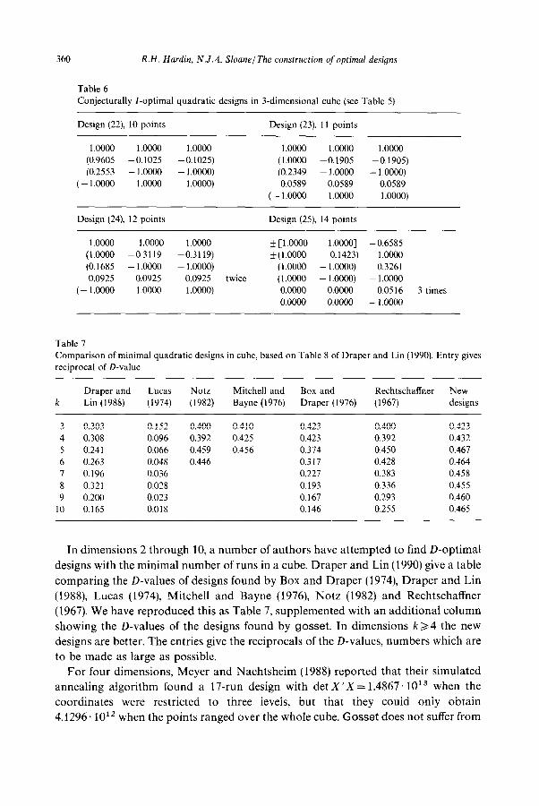
Table 6

Conjecturally I-optimal quadratic designs in 3-dimensional cube (see Table 5)

Design (22), 10 points Design (23) 11 points

1 .oooo 1.0000 1.0000 1.0000 1.0000 1.0000

(0.9605 -0.1025 -0.1025) (1.0000 -0.1905 -0.1905)

(0.2553 -1.0000 - 1.0000) (0.2349 -1.0000 - 1.0000)

( - 1 .oooo 1 .oOOO 1.0000) 0.0589 0.0589 0.0589

(-1.0000 1 .oooo 1.0000)

Design (24), 12 points Design (25), 14 points

1 .oOQo 1 .oooo 1 .oOOo + [l.OOOO 1 .OOOO] -0.6585

(I.0000 -0.3119 -0.3119) ~(1.0000 0.1423) 1 .oOQo

(0.1685 -1.0000 - 1 .OOcO) (1.0000 - 1 .OOOO) 0.3261

0.0925 0.0925 0.0925 twice (1.0000 - 1 .OOOO) - 1 .oooo

(-1.0000 1 .oooo 1 .OOOO) 0.0000 0.0000 -0.0516 3 times

0.0000 0.0006 - 1.0000

Table I

Comparison of minimal quadratic designs in cube, based on Table 8 of Draper and Lin (1990). Entry gives

reciprocal of D-value

Draper and Lucas Notz Mitchell and Box and Rechtschaffner New

k Lin (1988) (1974) (1982) Bayne (1976) Draper (1976) (1967) designs

3 0.303 0.152 0.400 0.410 0.423 0.400 0.423

4 0.308 0.096 0.392 0.425 0.423 0.392 0.432

5 0.241 0.066 0.459 0.456 0.374 0.450 0.467

6 0.263 0.048 0.446 0.317 0.428 0.464

7 0.196 0.036 0.227 0.383 0.458

8 0.321 0.028 0.193 0.336 0.455

9 0.200 0.023 0.167 0.293 0.460

10 0.165 0.018 0.146 0.255 0.465

In dimensions 2 through 10, a number of authors have attempted to find D-optimal

designs with the minimal number of runs in a cube. Draper and Lin (1990) give a table

comparing the D-values of designs found by Box and Draper (1974), Draper and Lin

(1988), Lucas (1974) Mitchell and Bayne (1976) Notz (1982) and Rechtschaffner

(1967). We have reproduced this as Table 7, supplemented with an additional column

showing the D-values of the designs found by gosset. In dimensions ka4 the new

designs are better. The entries give the reciprocals of the D-values, numbers which are

to be made as large as possible.

For four dimensions, Meyer and Nachtsheim (1988) reported that their simulated

annealing algorithm found a 17-run design with det X/X=1.4867. lOi when the

coordinates were restricted to three levels, but that they could only obtain

4.1296*10” when the points ranged over the whole cube. Gosset does not suffer from


this weakness, and found an even better continuous design, with

det X’X= 1.6863. 1013.

5.3. Linear designs in the cube

There is a substantial body of work dealing with the construction of designs

for linear regression in the k-dimensional cube (see for example Chadjipantelis

et al., 1987; Ehlich, 1964a, b; Ehlichj’and Zeller, 1962; Galil, 1985; Galil and Kiefer,

1980a, b,c, 1982a, b; Mitchell, 1974a, b; Moyssiadis and Kounias, 1982; Sathe and

Shenoy, 1989, 1991; Smith, 1988; Williamson, 1946; and the references therein).

The problem is to construct a design for the model /$, +fllxl + ... + /$x~, using

n > k+ 1 points in the unit k-dimensional cube, either restricting the points to

the vertices, or allowing them to range over the whole cube. For brevity we shall

concentrate on the case of minimal (or saturated) designs, with n = k + 1. Note that

in the case where both the measurement and modeling regions consist of the set of

vertices of the cube, the moment matrix A4 is the identity matrix, and A- and

I-optimality coincide.

The problem of finding a minimal D-optimal design in which the points are

restricted to the vertices of the cube can be rephrased as follows. Determine the value

of g(k+ l), the maximal determinant of any (k+ 1) x (k+ 1) matrix with entries +_ 1.

Many optimal designs are known for this problem, and these provide an opportunity

to evaluate the performance of our program in the case where all variables are discrete

(which is the most difficult for the algorithm).

We find that although the algorithm performs well up to about 20 dimensions,

finding the best designs known, in higher dimensions it does not perform as well as

programs such as that of Smith (1988) which are designed specifically for this problem.

Table 8 shows best lower bounds on g(k+ 1) presently known. In this

table, * indicates that the entry is known to be the exact value of g(k+ l), H

indicates a Hadamard matrix, G that gosset was able to find this design, Ch. et al. =

Chadjipantelis et al. (1987), E.(a) = Ehlich (1964a), E.(b) = Ehlich (1964b), E.Z. = Ehlich

and Zeller (1962) G.K. = Galil and Kiefer (1980a), M.K. = Moyssiadis and Kounias

(1982), S=Smith (1988), W. =Williamson (1946).

We also carried out a search for Z-optimal (or equivalently A-optimal) designs with

the same range of values of k. In each case we were able to find an Z-optimal design

which was also D-optimal, and we conjecture that this will always be true for minimal

designs. The converse is not always true. For k= 10 for example there are D-optimal

designs which are not Z-optimal (cf. Galil and Kiefer, 1980a, p. 12971). The Z-values of

these designs, normalized by division by k + 1, are shown in the last column of Table 8.

For some small values of k the designs change dramatically when the points are not

restricted to the vertices of the cube (and the measurement and modeling regions


Table 8 Best lower bound on maximal determinant of k l-matrix of order k + 1; and normalized I-value of conjecturally I-optimal design

k g(k+ 1) Notes I/F+ 1)

1 2 *, G 2 4 *, G 3 16 +, H, G 4 48 *, E.(a), E.(b), G 5 160 *, G 6 576 *, W, G 7 4096 *, H, G 8 14336 *, E.Z., G 9 73728 *, E.(a), E.(b), G

10 327680 *, E.Z., G.K., G 11 2985984 *> H, G 12 14929920 *, E.(a), E.(b), G 13 77635584 *, E.(a), E.(b), G 14 2418037760 S., G 15 4294967296 *, H, G 16 21474836480 *, M.K., G 17 146028888064 *, E.(a), E.(b), G 18 3894426939392 *, S. G 19 10240000000000 *, H, G 20 59392000000000 *, Ch. et al., G 21 2377073157799936 S. 22 22626567700217856 S. 23 36520347436056576 *, H

1 1.5 1 1.11111111 1.2 1.27777778

1.14795918 1.11111111 1.165 1 1.04 1.07692308 1.11142857 1 1.06 1.05882353 1.09527929 1 1.04447087

I

consist of the whole cube). For example, the following are conjecturally Z-optimal

designs for the cases k = 2 and 5:

where +=+l, -= -1, a=0.4391, b= -0.2417. Their Z-values are respectively

2 and 3.1986, compared with 2.5 and 3.2 for the *l-designs mentioned in

Table 8.

As a final example, we consider the problem of finding a D-optimal design for the

case k = 15, n = 19, which Galil (1985) mentions as unsolved. Equivalently, we wish to


Table 9 19 x 16 matrix X found by gosset, for which def X’X=2545*73

l-l -1 -1 -1 -1 1 -1 1 1 -1 -1 1 1 1 -1 l-l -1 -1 -1 1 1 1 -1 -1 -1 -1 1 -1 1 1 l-l -1 1 -1 1 1 1 -1 -1 1 -1 -1 1 1 1 l-l -1 1 1 -1 -1 1 1 1 1 1 1 1 -1 1 l-l -1 1 1 1 -1 -1 1 -1 -1 1 -1 -1 1 -1 l-l 1 -1 -1 1 1 1 1 -1 -1 1 1 -1 -1 1 l-l 1 -1 1 -1 1 -1 -1 1 1 1 -1 -1 1 1 l-l 1 -1 1 1 -1 -1 -1 -1 1 -1 1 1 -1 -1 l-l 1 1 -1 -1 -1 1 -1 1 -1 -1 -1 -1 -1 -1 1 1 -1 -1 -1 -1 -1 -1 1 -1 1 -1 -1 -1 -1 1 1 1 -1 -1 -1 1 -1 1 -1 1 1 1 1 -1 1 -1 1 1 -1 -1 1 -1 1 1 -1 -1 -1 1 -1 1 -1 -1 1 1 -1 1 -1 1 1 1 -1 1 1 1 -1 1 -1 -1 1 1 -1 1 1 1 1 -1 -1 1 -1 -1 1 -1 -1 1 1 1 1 -1 1 1 -1 1 1 1 -1 -1 -1 1 1 1 1 1 1 1 -1 -1 -1 -1 -1 -1 -1 1 1 1 1 1 1 1 1 1 -1 1 1 -1 1 -1 1 -1 1 1 -1 -1 1 1 1 1 -1 1 1 -1 1 1 -1 1 -1 1 1 1 1 1 1 1 1 -1 1 1 1 -1 1 -1 1 -1 1 -1

find a 19 x 16 f l-matrix X for which det X’X is maximal. The gosset program is

10 discrete xl x2 ... xl 5

20 model 1 +x1 +x2+ ... +x1 5

design runs = 19

and the matrix shown in Table 9 is the best of 4000 tries. It has

det X’X= 154473467218808012800=2545273.

5.4. A 'twisted' fractional factorial design

In the past year there have been numerous industrial and academic applications of

gosset. There is space for only one example here. This problem arose in studying

VLSI wafers, in an experiment with five quantitative discrete variables A, B, C, D,

E taking the values -1 and 1. The experimenter had manufactured 14 wafers, in which

A, B, C were set to 1, 1, 1 (twice), 1, 1, -1 (twice), and so on, excluding -1, -1, -1, but

in which the values of D and E were not yet chosen. The response surface model

involved main effects and all interactions except those mentioning C. The problem

was to determine what settings for D and E should be used on these same 14 wafers.

We ran gosset with the program . .

10 discreteABCDE-1 1

20 constraint A+B+C> -2.5

30 model l+A+B+C+D+E+A*B+A*D+A*E+B*D+B*E+D*E


where line 20 is used to exclude the values A = B = C = - 1, and asked for a design with

14 runs, guessing that this would produce a design meeting the requirements. It did. In

fact we obtained the same design whether we specified I-, D- or A-optimality.

Examination of the computer output showed that this presumably I-, D- and A-

optimal design can be regarded as a ‘twisted’ fractional factorial design with the

following definition: take all vectors A, B, C, D, E which satisfy ABCDE= -1, except

that if A = B = - 1, C = 1 the rule is ABCDE = 1, and then discard the two vectors with

A=B= C= - 1. Note that in the statement of the problem C is treated differently

from A and B, and the solution shows the same asymmetry. This experiment has now

been completed.

We are grateful to our colleagues L. Denby, A.E. Freeny and J.M. Landwehr for

telling us about this problem.

5.5. Designs for extrapolation

There have been a number of papers on designs for extrapolation, but these deal

mostly with the asymptotic theory (Galil and Kiefer, 1979; Hoel, 1965; Hoe1 and

Levine, 1964; Kiefer and Wolfowitz, 1964a, b, 1965). In this section we give some

examples of minimal or close to minimal designs.

These designs have not yet found application, but are included to illustrate the use

of gosset in situations in which the regions 0 and R are quite distinct, even disjoint.

Such designs must be used with care, for now it is harder to justify a polynomial

model. However, they illustrate one of the program’s more unusual features, the

technique could be modified to accommodate other models (it would be easy to

modify gosset to allow rational or trigonometric models), and the first of these

designs could arise in several situations.

The first example asks for a design which will fit a quadratic response surface to the

radiation level in a room with coordinates -1 <x< 1, O<y< 1, O<zb 1, with the

constraint that because of the high radiation level in the left half of the room,

measurements can only be made in the right half, i.e., in the region 0 d x, y, z < 1. The

gosset program is

10 rangexyzO1

20 range x’ -1 1

30 range y’ 2’ 0 1

40 model (1 +x’+y’+z’)^2

An example of a conjecturally I-optimal design with 13 runs is shown in

Table 10.

In another setting for this example, the x-coordinate is time, and we wish to

make measurements over a 24-hour period in order to model a response over

48 hours.


Table 10 Table 11

A 13-run design for fitting a quadratic

model in a room from measurements made

only in one half

Designs for extrapolation of cubic polynomial at a single

point (n is a number of observations)

n I-eff

0.0000 0.0000 0.0000 (0.0323

0.0000 0.5002

0.0000 0.8 162

0.5124 1 .oOOo

0.5132 (0.0000

0.5187 (0.0000

1 .oooo 0.0000

1 .oooo (0.3695

0.0000 1 .OOOO)

0.5002 0.8162 1 .ooOO

0.4361)

0.8448)

0.0000

0.9636)

Design

4 87.51 -1, -0.5798, 0.4689, 1

5 91.81 -1, - 0.5367, 0.47642, 1

6 94.07 -1, -0.5291, 0.5213’, 1’

10 99.50 -1, -0.49792, o.51194. l3

20 99.32 - 12, -0.5025’, 0.4854*, I 5 52 99.29 - 15, -0.499413, 0.4861 ‘I, 1’3

Many variations of these designs are possible. An extreme example might arise in

astronomy: find an I-optimal design for modeling a quadratic response on the moon

from measurements made on or in the earth. The gosset program is

10 sphere x y z radius 4000

20 sphere x’ y’ z’ radius 1000 center 240000 0 0

30 model (1 +x’+y’+z’)*2

and a lo-run (minimal) design consists of the points [3997, -154.0,37.5], [3992, 110.0,

230.71, [3991, 42.0, -268.11, [159, 158.9, -28.01, [154, -202.4, 47.73, [151, -107.2,

36.11, [136, 135.9, 200.31, [133, 16.4, -259.41, C-3997, 164.0, -7.01, C-3997, -164.9,

5.81.

Finally, we consider a l-dimensional extrapolation problem used as an illustration

by Hoe1 and Levine (1964): construct a design on C-1, l] to estimate a cubic

polynomial at the single point 2. It is shown in Hoe1 and Levine (1964) that the

Z-optimal design places respectively 5152, 12/52, 20152 and 15152 of the observations

at the points -1, - f, 1 and 1. We used the gosset program

10 range x

20 range x’ 1.99999 2.00001

30 model (1 +x)*3

to produce comparable designs, some of which are shown in Table 11.

We see that efficient designs are obtained even with small numbers of obervations.

Incidentally, although in the asymptotic theory Hoe1 and Levine (1964) show that the

same observation points can be used for extrapolation to any single point, our

program shows that in the finite theory this is not true.

The last two lines of the table show one of our algorithm’s limitations: because of

the way we move the design points, they all attempt to move to the most favorable

position, which tends to make them fall into ‘bunches’. The points in a bunch then stay


together throughout the iteration process. If there are a large number of points, many

more than in a minimal design, it may happen (as we have seen here) that there is

a vanishingly small chance of stumbling on the optimal distribution into bunches.

This does not occur with smaller numbers of observations, because then every

distribution has a significant probability of being tried.

Acknowledgements

We are extremely grateful to David H. Doehlert, whose letter to us (see Section 1)

triggered this work, and who has since provided invaluable guidance and encourage-

ment. During the course of this work we have also benefitted from discussions with

many of our colleagues at Bell Labs. In particular we should like to thank

A.R. Calderbank, A.E. Freeny, C.L. Mallows, V.N. Nair and D. Pregibon for their

advice. We are also grateful for comments and suggestions from R.B. Crosier, J.M.

Lucas. A.B. Owen and R.D. Tobias.

References

Atkinson, A.C. (1973). Multifactor second order designs for cuboidal regions. Biometrika 60, 15-19. Atwood, C.L. (1969). Optimal and efficient designs of experiments. Ann. Math. Statist. 40, 1570-1602. Bagchi, S. (1986). A series of nearly D-optimal third order rotatable designs. Sankhyii B. 48, 186-198.

Bajnok, B. (1991). Construction of spherical 4- and 5-designs. Graphs and Combin. 7, 219-233. Bajnok, B. (1992). Construction of spherical t-designs. Geometriae Dedicata, in press.

Becker, R.A., J.M. Chambers and A.R. Wilks (1988). The New S Language. Wadsworth and Brooks, Pacific

Grove, CA.

Beightler, C.S., D.T. Phillips and D.J. Wilde (1979). Foundations of Optimization. Prentice-Hall, Englewood

Cliffs, NY, 2nd ed.

Bose, R.C. and N.R. Draper (1959). Second order rotatable designs in three dimensions. Ann. Math. Statist. 30, 1097-1112.

Box, G.E.P. and D.W. Behnken (1960a). Simplex-sum designs: a class of second order rotatable designs

derivable from those of first order. Ann. Math. Statist. 31, 838-864.

Box, G.E.P. and D.W. Behnken (1960b). Some new three level designs for the study of quantitative

variables. Technometrics 2, 455-475. Box, G.E.P. and N.R. Draper (1959). A basis for the selection of a response surface design. J. Amer. Statist.

Assoc. 54, 622-654. Box, G.E.P. and N.R. Draper (1963). The choice of a second order rotatable design. Biometrika SO, 335-352. Box, G.E.P. and N.R. Draper (1987). Empirical Model-Building and Response Surfaces. Wiley, New York.

Box, G.E.P. and J.S. Hunter (1957). Multi-factor experimental designs for exploring response surfaces. Ann. Math. Statist. 28, 195-241.

Box, M.J. and N.R. Draper (1971). Factorial designs, the JX’XI criterion and some related matters.

Technometrics 13, 731-742. Box, M.J. and N.R. Draper (1974). On minimum-point second-order designs. Technometrics 16, 613-616. Chadjipantelis, T., S. Kounias and C. Myssiadis (1987). The maximum determinant of 21 x 21 (+ 1, -l)-

matrices and D-optimal designs. J. Statis. Plann. Inference, 16, 167-178.

Chambers, J.M. and T.J. Hastie, eds. (1991). Statistical Models in S. Wadsworth and Brooks, Pacific Grove,

CA.

Conway, J.H. and N.J.A. Sloane (1988). Sphere Packings, Lattices and Groups. Springer-Verlag. New York.


Conway, J.H. and N.J.A. Sloane (1991). The cell structures of lattices. In: P. Hilton et al., eds., Misceilanea mathematics. Springer-Verlag, New York, pp. 71- 107.

Cook, R.D. and C.J. Nachtsheim (1980). A comparison of algorithms for constructing exact D-optimal

designs. Technometrics 22, 315-324. Cornell, J.A. (1990). Experiments with Mixtures. Wiley, New York, 2nd ed.

Coxeter, H.S.M. (1973). Regular Polytopes. Dover, New York, 3rd ed.

Crary, S.B. (1991). Optimal design of experiments for sensor calibration. in: Proc. 1991 Internat. Conf: Solid-State Sensors and Actuators (San Francisco, June 23-27. 1991).

Crosier, R.B. (1991). Some New Three-Level Response Surface Designs. Report CRDEC-TR-308, U.S. Army

Chemical Research, Development & Engineering Center, Aberdeen Proving Ground, MD.

Delsarte, P., J.M. Goethals and J.J. Seidel (1977). Spherical codes and designs. Geometriae Dedicata 6,

363-388. Dodge, Y., V.V. Fedorov and H.P. Wynn (1988). Optimal design of experiments: An overview. In: Y. Dodge

et al., eds., Optimal Design and Analysis of Experiments. North-Holland, Amsterdam, pp. l- 11.

Doehlert, D.H. (1970). Uniform shell designs, J. Roy. Statist. Sot., Ser. C, 19, 231-239.

Doehlert, D.H. and V.L. Klee (1972). Experimental designs through level reduction of the d-dimensional

cuboctahedron. Discrete Math. 2, 309-334. Draper, N.R. (1960). Second order rotatable designs in four or more dimensions. Ann. Math. Statist. 31,

23-33. Draper, N.R. and D.K.J. Lin (1988). Using Plackett and Burman Designs With Fewer Than N-l Factors.

Technical Report 848, Department of Statistics, Univ. of Wisconsin, Madison, WI.

Draper, N.R. and D.K.J. Lin (1990). Small response-surface designs. Technometrics 32, 187-194. Draper, N.R. and F. Pukelsheim (1990). Another look at rotatability. Technometrics 32, 195-202. Ehlich, H. (1964a). Determinantenabschitzungen fiir binire Matrizen. Math. Zeit 83, 123-132. Ehlich, H. (1964b). Determinantenabschatzungen fiir binire Matrizen mit n=3 mod 4. Math. Zeit 84,

438-447. Ehlich, H. and K. Zeller (1962). Binire Matrizen. Zeit. Angew. Math. Mech. 42, 20-21. Farmakis, N. (1991). Constructions of A-optimal weighing designs when n= 19. J. Statist. Plann. Infer. 27,

249-261. Farrell, R.H., J. Kiefer and A. Walbran (1967). Optimum multivariate designs. In: Pror. 5th Berkeley

Sympos. Math. Statist. and Probability, Univ. Calif. Press, Berkeley, CA, 1, pp. 113-138.

Galil, Z. (1985). Computing D-optimum weighing designs: Where statistics, combinatorics, and computa-

tion meet. In: L.M. Le Cam and R.A. Olshen, eds., Proceedings Berkeley Conference in Honor of Jerzy Neyman and Jack Kiefer. Wadsworth, Monterey, CA., Vol. II, pp. 635-650.

Galil, Z. and J. Kiefer (1977a). Comparison of rotatable designs for regression on balls, I (quadratic). J. Statist. Plann. Infer. 1, 21-40.

Galil, Z. and J. Kiefer (1977b). Comparison of design for quadratic regression on cubes. J. Statist. Plann. Infer. 1, 121-132.

Galil,, Z. and J. Kiefer (1979) Extrapolation designs and @,-optimum designs for cubic regression on the

q-ball. J. Statist. Plann. Infer. 3, 27-38. Galil, 2. and J. Kiefer (1980a). D-optimum weighing designs. Ann. Statist. 8, 1293-1306.

Galil, Z. and J. Kiefer (1980b). Time- and space-saving computer methods, related to Mitchell’s DETMAX,

for finding D-optimum designs. Technometrics 22, 301-313. Galil, Z. and J. Kiefer (1980~). Optimum weighing designs, In: K. Matusita, ed., Recent Developments in

Statistical Inference and Data Analysis. North-Holland, Amsterdam, pp. 183-189.

Galil, Z. and J. Kiefer (1982a). On the characterization of D-optimum weighing designs for n = 3 (mod 4). In:

S.S. Gupta and J.O. Berger, eds., Statistical Decision Theory and Related Topics III. Academic Press, New York, Vol. 1, pp. l-35.

Galil, Z. and J. Kiefer (1982b). Construction methods for D-optimum weighing designs when n = 3 (mod 4).

Ann. Statist. 10, 502-510.

Giovannitti-Jensen, A. and R.H. Myers (1989). Graphical assessment of the prediction capability of response surface designs. Technometrics 31, 159-171.

Haines, L.M. (1987). The application of the annealing algorithm to construction of exact optimal designs for

linear regression models. Technometrics 29, 439-447.

368 R.H. Hardin, N.J.A. SloaneJThe construction of optimal designs

Hardin, R.H. and N.J.A. Sloane (1992). Operating Manual for Gosset: A General-Purpose Program for Constructing Experimental Designs (Second Edition). Statistics Research Report, AT&T Bell Laborator-

ies, Murray Hill, NJ.

Hardin, R.H. and N.J.A. Sloane (1992a). Computer-Generated Minimal (and Larger) Response-Surface Designs: (I) The Sphere, Statistics Research Report, AT&T Bell Laboratories, Murray Hill, NJ.

Hardin, R.H. and N.J.A. Sloane (1992b). Computer-Generated Minimal land Larger) Response-Surface Designs: (II) The Cube. Statistics Research Report, AT&T Bell Laboratories, Murray Hill, NJ.

Hardin, R.H.and N.J.A. Sloane (1992~). Tables of Experimental Designs. Statistics Research Report, AT&T

Bell Laboratories, Murray Hill, NJ.

Hardin, R.H. and N.J.A. Sloane (1992d). New spherical 4-designs. Discrete Math., 106/107, 255-264. Hardin, R.H. N.J.A. Sloane and Warren D. Smith (1993). Spherical Codes. In preparation.

Herzberg, A.M. (1967). A method for the construction of second order rotatable designs in k dimensions. Ann. Math. Statist. 38, 177-180.

Hoel, P.G. (1965). Optimum designs for polynomial extrapolation. Ann. Math. Statist. 36, 1483-1493. Hoel, P.G. and A. Levine (1964). Optimal spacing and weighting in polynomial prediction. Ann. Math.

Statist. 35, 1553-1560. Hooke, R. and T.A. Jeeves (1961). ‘Direct search’ solution of numerical and statistical problems. J. Assoc.

Comp. Machinery 8, 212-229. Huda, S. (1982). Some third-order rotatable designs. Biom. J. 24, 257-263. Huda, S. (1983). Two third-order rotatable designs in four dimensions. J. Statist. Plann. Infer. 8, 241-243. Hume, A.G. and M.D. McIlroy (1990). UNIX Research System, Tenth edition. AT&T Bell Laboratories,

Murray Hill, NJ, Vol. II.

Kiefer, J. (1960). Optimum experimental designs V, with applications to systematic and rotatable designs.

In: Proc 4th Berkeley Sympos. Math. Statist. and Probability, Univ. Calif. Press. CA. 1, pp. 381-405.

Kiefer, J. (1985). Collected Papers III: Design of Experiments. L.D. Brown et al., eds., Springer-Verlag,

New York.

Kiefer, J. and J. Wolfowitz (1960). The equivalence of two extremum problems. Canad. J. Math. 12, 363-366.

Kiefer, J. and J. Wolfowitz (1964a). Optimum extrapolation and interpolation designs I. Ann. Inst. Statist.

Math. 16, 79-108.

Kiefer, J. and J. Wolfowitz (1964b). Optimum extrapolation and interpolation designs II. Ann. Inst. Statist. Math. 16, 295-303.

Kiefer, J. and J. Wolfowitz (1965). On a theorem of Hoe1 and Levine on extrapolation designs. Ann. Math. Statist. 36, 1627-1655.

Lucas, J.M. (1974). Optimum composite designs. Technometrics 16, 561-567. Lucas, J.M. (1976). Which response surface design is best. Technometrics 18, 411-417.

Lucas, J.M. (1977). Design efficiencies for varying numbers of centre points. Biometrika 64, 145-147. Meyer, R.H. and C.J. Nachtsheim (1988). Constructing exact D-optimal experimental designs by simulated

annealing. Amer. J. Math. Management Sci. 8, 329-359. Mitchell, T.J. (1974a). An algorithm for the construction of ‘D-optimal’ experimental designs. Technometrics

16, 203-210. Mitchell, T.J. (1947b)‘. Computer construction of ‘D-optimal’ first-order designs. Technometrics 16,

211-220. Mitchell, T.J. and C.K. Bayne (1976). D-optimal Fractions of Three Leuel Factorial Designs. Report CSD-19,

Oak Ridge National Laboratory, Oak Ridge, TN. Mitchell, T.J. and C.K. Bayne (1978). D-optimal fractions of three-level factorial designs. Technometrics 20,

369-380. Moyssiadis, C. and S. Kounias (1982). The exact D-optimal first order saturated design with 17 observa-

tions. J. Statist. Plann. Infer. 7, 13-27. Myers, R.H., A.I. Khuri and W.H. Carter Jr. (1989). Response surface methodology: 1966-1988.

Technometrics 31, 137- 157. Nachtsheim, C.I. (1987). Tools for computer-aided design of experiments. J. Qual. Technol. 19, 132-160. Neumaier, A. and J.J. Seidel (1992). Measures of strength 2e, and optimal deigns of degree e. Sankhyii, to

appear.


Notz, W. (1982). Minimal poinl second order designs. J. Statist. Plann. Infer. 6, 47-58.

Pearson, E.S. and J. Wishart eds. (1942). “Students” Collected Papers. University College, London.

Pesotchinsky, L.L. (1975). D-optimum and quasi-D-optimum second-order designs on a cube. Biomerrika

62, 335-340. Rabau, P. and B. Bajnok (1991). Bounds for the number of nodes in Chebyshev type quadrative formulas.

J. Approx. Theory 67, 199-214. Rechtschaffner, R.L. (1967). Saturated fractions of 2” and 3” factorial designs. Technometrics 9, 569-575. Roquemore, K.G. (1976). Hybrid designs for quadratic response surfaces. Technomerrics 18, 419-423. St. John, R.C. and N.R. Draper (1975). D-optimality for regression designs: A review. Technometrics 17,

15-23. Sathe, Y.S. and R.G. Shenoy (1989). A-optimal weighing designs when N ~3 (mod 4). Ann. Statist. 17,

1906&1915.

Sathe, Y.S. and R.G. Shenoy (1991). Further results on construction methods for some A- and D-optimal

weighing designs when N = 3 (mod 4). J. Statist. Plann. Infer. 2& 339-352. Seymour, P.D. and T. Zaslavsky (1984). Averaging sets: A generalization of mean values and spherical

designs. Advances in Math. 52, 213-240.

Warren D. Smith (1988). Studies in Computational Geometry Motivated by Mesh Generation. Ph.D.

dissertation, Princeton Univ., NJ.

Snow, M.E. and S.B. Crary (1991). The use of simulated annealing in the I-optimal design of experiments.

The Michigan Academician, submitted.

Steinberg, D.M. and W.G. Hunter (1984). Experimental design: Review and comment. Technometrics 26, 71-97.

Sudden, W.J. (1977). Optimal designs for integrated variance in polynomial regression. in: S.S. Gupta and

D.S. Moore, eds., Stafistical Decision Theory and Related Topics II. Academic Press, pp. 41 l-420.

Vining, G.G. (1990). A Computer Programfor Generating Variance Dispersion Graphs. Technical Report 373,

Dept. Statistics, Univ Florida, Gainesville, FL.

Vuchkov, I.N., D.L. Damgaliev and C.A. Yontchev (1981). Sequentially generated second order quasi

D-optimal designs for experiments with mixture and process variables. Technometrics 23, 233-238. Welch, W.J. (1982). Branch-and-bound search for experimental designs based on D-optimality and other

criteria. Technometrics 24, 41-48. Williamson, J. (1946). Determinants whose elements are 0 and 1. Amer. Math. Monthly 53, 427-434. Yonchev, H. (1988). New computer procedures for constructing D-optimal designs, An overview. In:

Y. Dodge et al., eds., Optimal Design and Analysis qfExpriments, North-Holland, Amsterdam, pp. 71-80.

a new approach to the construction of optimal designsneilsloane.com/doc/me175.pdf · r.h. hardin,...

Documents