A New Approach to Identifying the Real Effects ofUncertainty Shocks

Minchul ShinUniversity of Illinois

Molin Zhong∗

Federal Reserve Board

This version: May 6, 2018

Abstract

This paper introduces the use of the sign restrictions methodology to identify un-certainty shocks. We apply our methodology to a class of vector autoregression modelswith stochastic volatility that allow volatility fluctuations to impact the conditionalmean. We combine sign restrictions on the conditional mean and conditional secondmoment impulse responses to identify financial and macro uncertainty shocks. OnU.S. data, we find stronger evidence that financial uncertainty shocks lead to a declinein real activity and an easing of the federal funds rate relative to macro uncertaintyshocks.

Key words: Uncertainty, sign restrictions, vector autoregression, volatility-in-mean, Wishartprocess, multivariate stochastic volatility.

JEL codes: C11, C32, E32

∗Minchul Shin: 214 David Kinley Hall, 1407 W. Gregory, Urbana, Illinois 61801. E-mail: minc-shin@illinois.edu. Molin Zhong: 20th Street and Constitution Avenue N.W., Washington, D.C. 20551.E-mail: molin.zhong@frb.gov. We are grateful for the advice of our advisors Frank Diebold, Jesus Fernandez-Villaverde, and Frank Schorfheide. We especially would like to thank the editor and associate editor, threeanonymous referees, and our discussants Drew Creal and Soojin Jo. We also thank Pooyan Amir-Ahmadi,Jonas Arias, David Arseneau, Ross Askanazi, Dario Caldara, Todd Clark, Thorsten Drautzburg, Bora Durdu,Rochelle Edge, Luca Guerrieri, Pablo Guerron-Quintana, Mohammad Jahan-Parvar, Jihyung Lee, ChristianMatthes, Michael McCracken, Juan Rubio-Ramırez, Chiara Scotti, Jacob Warren, Shu Wu, Tao Zha, aswell as seminar participants at the Federal Reserve Bank of Kansas City, University of Illinois, Universityof Kansas, Penn Econometrics reading group, Federal Reserve Board, Midwest Econometrics Group 2015,Midwest Macro Meetings 2015, SNDE 2016, NASM Econometric Society 2016, IAAE 2016, System MacroMeetings 2016, and NBER EFSF Fall Meetings 2016 for useful comments. The views expressed in this paperare solely the responsibility of the authors and should not be interpreted as reflecting the views of the Boardof Governors of the Federal Reserve System or of any other person associated with the Federal ReserveSystem.

1

2

1 Introduction

What are the real effects of uncertainty on the macroeconomy? This question has been chal-

lenging to answer empirically. Since the seminal paper by Bloom (2009), many papers have

taken a variety of approaches including using uncertainty proxies (Baker et al., 2013; Scotti,

2013; Bachmann et al., 2013; Carriero et al., 2015), structural macro models (Fernandez-

Villaverde et al., 2011; Leduc and Liu, 2012; Born and Pfeifer, 2014; Basu and Bundick,

2015; Fernandez-Villaverde et al., 2015; Schorfheide et al., 2016), and two-step factor esti-

mation (Jurado et al., 2015; Ludvigson et al., 2015). Two important issues that come to

the fore are that uncertainty is not observed and that different sources of uncertainty may

affect agents’ decisions in different ways. One would ideally desire an econometric framework

that can both accurately measure uncertainty from the data and identify different sources

of uncertainty shocks.

In this paper, we propose a new strategy to identify the real effects of uncertainty shocks

that seeks to simultaneously address both empirical issues. We analyze a class vector autore-

gressive (VAR) models with multivariate stochastic volatility that allow for the volatility-

in-mean effect. VAR models with stochastic volatility-in-mean have been considered by a

variety of papers, including Mumtaz and Zanetti (2013), Jo (2014), Creal and Wu (2017),

Mumtaz and Theodoridis (2016), and Carriero et al. (2017a). These models have been useful

in providing a unifying framework to measure uncertainty and its real effects.

We bring to this literature the use of sign restrictions (Faust, 1998; Canova and Nicolo,

2002; Uhlig, 2005) on the mean and volatility responses of observed economic variables to an

uncertainty shock of interest. The literature on sign restrictions to identify level structural

shocks in VARs is well developed. Important recent theoretical advances include Baumeister

and Hamilton (2015); Arias et al. (2014); Giacomini and Kitagawa (2015); Moon et al. (2017);

Amir-Ahmadi and Drautzburg (2017). Our paper, however, is the first to consider the use

sign restrictions on the volatility equation to identify structural second moment shocks, in

3

contrast to its previous use to identify structural first moment shocks. The uncertainty

shocks considered in our paper are different from level shocks because uncertainty shocks

impact both the conditional mean of variables as well as conditional second moment objects

of interest, including the volatility of the VAR innovations and the forecast error variances of

the variables. With this insight in hand, we proceed to use sign restrictions on the responses

of both first and second moment responses to identify our structural uncertainty shocks,

which is new to the sign restrictions literature. As we show in an example in the paper, sign

restrictions on the first moment and second moment responses each provide useful identifying

information.

Our approach is also novel when viewed in the context of the volatility-in-mean literature.

Previous papers, such as Mumtaz and Zanetti (2013) and Jo (2014), initially identify first

moment structural shocks and then put stochastic volatility on those shocks. Our comple-

mentary approach views the level equation of the VAR as a flexible way to control for the

expected movements of our macro variables of interest in order to more accurately measure

conditional volatility, as emphasized by Jurado et al. (2015). The heart of our identification

problem comes from considering the correlated innovations in the volatility equation. In this

sense, our work has much in common with Creal and Wu (2017) and Carriero et al. (2017a),

who both face a similar problem. These latter two papers solve the second moment identifi-

cation problem by recursive ordering assumptions. Mumtaz and Theodoridis (2016) do not

have an identification problem for uncertainty shocks, as they specify a factor structure for

volatility with a single volatility factor.

A quite general class of volatility models are compatible with our methodology. Our

framework is amenable to many of the volatility processes popular in the literature, including

Cholesky-type decompositions (Cogley and Sargent, 2005; Primiceri, 2005), factor volatility,

and level shocks impacting volatility (Carriero et al., 2017a). We consider as a benchmark

case the conditional autoregressive inverse Wishart (CAIW) model. This volatility process,

introduced into the financial econometrics literature by Golosnoy et al. (2012) and in macroe-

4

conomics by Karapanagiotidis (2012) and Rondina (2012), models time-varying volatility

with the Wishart family of distributions (See Philipov and Glickman, 2006; Gourieroux

et al., 2009; Fox and West, 2013, for alternative autoregressive Wishart models.). We find

this model attractive because of its flexibility and property that its estimation results do not

depend on the ordering of the observable variables in the system. Moreover, the volatility

process can be written linearly in terms of the one-step-ahead forecast error variances and

covariances, which facilitates the imposition of sign restrictions on the volatility responses.

As an illustration of our empirical framework, we identify the real effects of financial ver-

sus macro uncertainty shocks with two examples. Across these two examples, we emphasize

the importance of spreads in distinguishing between different uncertainty shocks, which is

novel to the literature. Namely, we find that the uncertainty shock that increases spreads

more leads to stronger evidence of a decline in industrial production and subsequent reaction

of the federal funds rate. Our work, therefore, complements Caldara et al. (2016) in that

it emphasizes the centrality of spread behavior and financial markets in understanding un-

certainty shocks. The difference is that we use spreads to differentiate two second moment

shocks. Our alternative identification assumption also adds to the discussion on identifying

financial and macro uncertainty shocks (Carriero et al., 2017a; Ludvigson et al., 2015).

Our first example uses a small four-variable monetary VAR with a CAIW model of volatil-

ity and industrial production, the consumer price index, the federal funds rate, and the excess

bond premium (EBP) of Gilchrist and Zakrajsek (2012). Financial and macro uncertainty

shocks are both assumed to increase the volatilities of all innovations in the economy. The

key distinguishing feature is that a financial uncertainty shock is assumed to increase the

excess bond premium by more than the macro uncertainty shock. We assume a conditional

Haar prior over the rotation matrix and conduct an extensive analysis of the prior impli-

cations for the impulse response functions (IRF) and an identified set analysis (Baumeister

and Hamilton, 2015; Moon et al., 2017). We find more evidence that a financial uncertainty

shock leads to a decline in industrial production relative to a macro uncertainty shock. We

5

also find that a financial uncertainty shock increases the forecast error variance of industrial

production and EBP more than a macro uncertainty shock does.

Our second example asks whether we can robustly identify the effects of financial and

macro uncertainty shocks in the sense of Giacomini and Kitagawa (2015). Robust sign

restrictions account for the implications of all possible priors over the rotation matrices, and

hence are immune to the concerns of Baumeister and Hamilton (2015). In considering the

robust implications of these two types of uncertainty shocks, we find it necessary to improve

our estimation of financial and macro volatility. Therefore, we turn to the model of Carriero

et al. (2017a), which is a state-of-the-art volatility factor model. Carriero et al. (2017a)

estimate financial and macro volatility factors as the common movements of volatility across

a set of 30 macro and financial data series, respectively. The model additionally allows for

level shocks to impact volatility as well, thereby controlling for a potentially important source

of volatility fluctuations. We impose a similar set of sign restrictions, with a key condition

being that a financial uncertainty shock leads to a larger rise in the BAA-10 year Treasury

spreads relative to a macro uncertainty shock. The results are largely consistent with those

from the small VAR model. There is strong evidence suggesting that industrial production

declines following a financial uncertainty shock, but less support for such a decline following

a macro uncertainty shock. Moreover, we also find that a financial uncertainty shock leads

to a decline in the federal funds rate, while we find little evidence that a macro uncertainty

shock does.

The plan of the paper is as follows. In section 2, we present our general empirical frame-

work, discuss the volatility identification problem, and lay out our sign restrictions strategy

to identify uncertainty shocks. In section 3, we discuss various volatility processes that are

amenable to our framework and compare our work with the extant literature. Section 4

contains a discussion of inference issues, including the identification problems introduced by

sign restrictions. Section 5 contains our empirical illustration on the effects of financial and

macro uncertainty shocks and Section 6 concludes.

6

2 Empirical Framework

2.1 Model

We analyze VAR models with stochastic volatility in which the volatility movements may

impact the conditional mean.

We begin with a general framework that encompasses many popular models in the lit-

erature. Consider the following non-linear VAR for a vector of economic variables yt =

[y1,t, y2,t, ..., yn,t]′,

yt = µy + Φyyt−1 +Bygy(Σt) + εt, εt|Ft−1,Σt ∼i.i.d. N (0, Σt) (1)

Σt = f(ht;A) (2)

ht = µh + Φhht−1 +Bhgh(Yt−1) + vt, vt|Ft−1 ∼m.d.s. V(0,Ωt) (3)

where Σt is a positive definite n×n matrix and ht is a k×1 vector. The function gy(·) takes

an n× n matrix and returns an l × 1 vector and gh(·) takes an n× 1 vector and returns an

m×1 vector. The function f(·;A) with parameter matrix A takes an k×1 vector and returns

an n×n matrix and its inverse mapping f−1(Σt, A) = ht is assumed to be well-defined on the

support of A. A primary example for this function in the literature is f(ht;A) = Adiag(ht)A′

where A is a k×k lower triangular matrix with ones on the diagonal. µy and µh are constant

vectors with dimensions n× 1 and k × 1, respectively. The coefficient matrices Φy, By, Φh,

Bh govern the dynamic relationships among the elements in [y′t, h′t]′. We can allow for lags

on these coefficient matrices as well, which we do in our empirical application.

There are two types of innovation vectors, εt and vt. The innovation εt is a vector of

shocks on the yt equation and is identically and independently distributed (iid) as the mul-

tivariate normal distribution with mean zero and variance-covariance matrix Σt conditional

on the time t− 1 information set Ft−1 = yt−1,Σt−1, yt−2,Σt−2, ... and Σt. Another type of

7

innovation vt, on the ht equation, is a vector of martingale difference sequences with respect

to Ft−1 and its conditional distribution V has mean zero and variance-covariance matrix Ωt,

whose elements are deterministic transformations of ht−1 and parameter ω, Ωt = Ω(ht−1;ω).

We let the conditional distribution of vt be slightly more general than the conditional dis-

tribution of εt to maintain the positive definiteness of Σt almost surely. For many volatility

processes, the distribution of vt is i.i.d. multivariate normal.

Of key interest in our investigation is the n × n matrix Σt = V ar(yt|Ft−1,Σt), which is

the conditional variance-covariance of yt conditional on the past information set Ft−1 and

Σt. This is the one-step-ahead forecast error variance-covariance of the economic variables

(yt) formed by economic agents at time t (e.g. in DSGE models). It is time-varying and

intimately related with the uncertainty economic agents have over the observables yt. Our

empirical framework allows for two sources of volatility fluctuations: exogenous shocks to

volatility vt and endogenous responses of volatility to past movements of economic variables

Bhgh(yt−1). In our paper, we are specifically focused on measuring the macroeconomic

implications of the former.

Many of the papers in the literature, including Mumtaz and Zanetti (2013), Jo (2014),

and Carriero et al. (2017a), fall into this general class of models. Creal and Wu (2017)

is a consequential related paper that adopts an alternative timing assumption that allows

time t volatility Σt to be determined after time t level shocks εt. We leave a discussion

of the commonalities and differences between our setup and previous papers for the next

section. A salient point, however, is that as long as some nonlinear transformation of Σt,

ht = f−1(Σt;A), admits a linear structure, our idea developed in this section applies.

There are several important practical issues that complicate the analysis. First, econo-

metricians do not observe Σt directly. Therefore, we must use equations 1, 2, and 3 to infer

volatility from the observable data y1:T . The equation with yt is as in a standard VAR except

that 1) the conditional variance of its innovations are stochastic and time-varying and 2) the

conditional variance enters the conditional mean equation.

8

Second, just as in the standard linear VAR for yt without stochastic volatility and its in-

mean effect, there is a shock labeling issue when we have more than one source of volatility

fluctuations. Without further assumptions, elements in the vector vt are correlated contem-

poraneously, which makes it difficult to interpret impulse response functions and variance

decompositions in terms of vt shocks. An increase in one of the elements in vt (e.g., the

volatility of the innovation to industrial production) is potentially due to different sources

(e.g., either uncertainty originating in the real economy or the financial markets). The prin-

cipal difference with most of the literature, however, is that this shock labeling issue is over

second moment as opposed to first moment shocks.

2.2 Identification of uncertainty shocks

In this section, we discuss how we can distinguish various sources of fluctuations in the

economic variables’ forecast error variances and covariances (Σt) using a sign restrictions

methodology. In the structural VAR language, we identify contemporaneously uncorrelated

shocks that affect Σt and study how these isolated shocks impact yt and Σt over time. Our

key observation is that the linear VAR framework for ht (equation 3) naturally allows us

to use the identification strategies developed in the structural VAR literature to identify

uncertainty shocks. It allows us to put identifying restrictions directly on the uncertainty

shocks. In this manner, we can focus on identifying uncertainty shocks alone, which are

the objects we are interested in. Our discussion in this section is based on fixed model

parameters and volatility processes, ψ = (µy,Φy, By, µh,Φh, Bh, ω, h1:T ).

Shock labeling problem. We first assume that the time t volatility innovation (vt) is a

linear function of uncorrelated unit-variance shocks (v∗t ), so we have

vt = Rtv∗t or R−1

t vt = v∗t , (4)

9

where Rt is a k × k invertible matrix with RtR′t = Ωt. The mean of v∗t is zero and the

conditional variance-covariance matrix is an identity matrix, E(v∗t v∗′t |Ft−1) = Ik. We call v∗t

as “structural” uncertainty shocks. Unlike vt, each element in v∗t is uncorrelated with each

other. Therefore, we can isolate the effect of one element in v∗t from another, making the

analysis of uncertainty shocks more intuitive and interpretable. Unlike first moment shocks,

our uncertainty shocks v∗t have a contemporaneous impact on both the stochastic covariance

matrix (Σt) as well as the conditional mean of the observed variables (yt).

Impulse response function. Our empirical framework allows uncertainty shocks to affect

both Σt and yt. We therefore consider first moment impulse response functions and second

moment impulse response functions.

A first moment impulse response function gives the expected change in the conditional

means of the observable variables from the jth structural uncertainty shock v∗t = ej (ej is a

column vector of length k with a 1 in the jth element and zeros elsewhere),

IRF [yi,t+s|v∗t = ej;Rt, ψ] = E(yi,t+s|v∗t = ej;Rt, ψ)− E(yi,t+s|v∗t = 0k×1;Rt, ψ) (5)

for s ≥ 0. This captures the s-step-ahead response of the ith variable to the jth uncertainty

shock. The expectation is taken with respect to the joint distribution of the future realization

of shocks in the system conditional on vt and Ft−1, [vt+1, vt+2, ..., vt+s]′ and [εt, εt+1, ..., εt+s]

′.

Depending on the specification of the volatility process, Ωt may depend on ht−1, making

the IRFs path dependent. We denote the time period in which the uncertainty shock is

considered by the time subscripts on v∗t and Rt.

A second moment impulse response function gives the expected change in the conditional

variance covariance matrix (or potentially a convenient transformation of the variance co-

variance matrix) of the innovations to the observable variables (yt) from the jth uncertainty

10

shock v∗t = ej. First we define

IRF [Σii,t+s|v∗t = ej;Rt, ψ] = E (Σii,t+s|v∗t = ej;Rt, ψ)− E (Σii,t+s|v∗t = 0k×1;Rt, ψ) (6)

for s ≥ 0. This captures the s-step-ahead impact of the jth uncertainty shock realized at

time t on the economic agents’ forecast error variance about variable yi,t+s formed at time

t+ s. This forecast error variance is at the time before they make a decision, but after they

observe Σt+s.

A more interpretable second moment impulse response function is in terms of the forecast

error variance as defined in Jurado et al. (2015):

IRF[FEV (yi,t+s)

∣∣v∗t = ej;Rt, ψ]

= V ar(yi,t+s

∣∣v∗t = ej;Rt, ψ)−V ar

(yi,t+s

∣∣v∗t = 0k×1;Rt, ψ)

(7)

for s ≥ 0. This is the s-step-ahead impact of the jth uncertainty shock realized at time t

on the economic agents’ s-step-ahead forecast error variance about variable yt+s formed at

time t.

It is important to note that these second moment response functions may be different

from the impulse response functions for ht:

IRF [hi,t+s|v∗t = ej;Rt] = E (hi,t+s|v∗t = ej;Rt, ψ)− E (hi,t+s|v∗t = 0k×1;Rt, ψ) (8)

for s ≥ 0. In general, imposing restrictions on ht leads to different implications compared to

the case of imposing restrictions on Σt.

Putting sign restrictions to restrict the set of admissible Q. The relationship be-

tween volatility innovations vt and structural uncertainty shocks v∗t is not uniquely pinned

down by equation 4. In fact, any Rt with Rt = Ω1/2t Q where Q ∈ O(k) = Q : QQ′ = Q′Q =

Ik, Q is a k×k matrix and Ω1/2t = chol(Ωt) would satisfy the relationship. This implies that

11

we have a range of impulse responses of variables of interest to uncertainty shocks even at

a fixed model parameter ψ. Moreover, without further assumptions, we cannot differentiate

the effect of one uncertainty shock from another: the range of possible impulse response

functions is the same for all uncertainty shocks.

To overcome this problem, we look for restrictions that can be imposed on the signs of the

first and second moment IRFs. These economic restrictions ideally would come from eco-

nomic theory or outside empirical evidence. Imposing economic restrictions on the responses

to the uncertainty shocks v∗t involves conditions on the set of IRFs that we consider.

Intuitively, the idea of applying sign restrictions to identify uncertainty shocks involves

choosing constraints on the signs of the first and second moment responses to the shock of

interest. Restrictions on the signs of these level impulse response functions we label as first

moment restrictions while those on the signs of volatility-related impulse response functions

we call second moment restrictions.

The first moment restrictions can be written as

ryi,j,s,t × IRF [yi,t+s|v∗t = ej;Rt, ψ] ≥ 0, (9)

where ri,j,s,t = −1, 0, 1. For example, if ri,j,s,t = −1, then this restriction implies that

the s-step-ahead response of the ith variable to the jth uncertainty shock realized at time

t is restricted to be negative. If ri,j,s,t = 0, then the sign restriction is not imposed on this

response. Similarly, we can write second moment restrictions as

rΣi,j,s,t × IRF [Σii,t+s|v∗t = ej;Rt, ψ] ≥ 0

rFEVi,j,s,t × IRF [FEV (yi,t+s)|v∗t = ej;Rt, ψ] ≥ 0

rhi,j,s,t × IRF [hi,t+s|v∗t = ej;Rt, ψ] ≥ 0.

(10)

We define a sign restriction set, R, which collects non-zero ryi,j,s,t, rΣi,j,s,t, r

FEVi,j,s,t, and rhi,j,s,t for

12

all i, j, s, and t. This set contains all information about the imposed sign restrictions.

The first and second moment economic restrictions are conditions on the set of impulse

response functions following the jth uncertainty shock. These conditions imply restrictions

on the admissible set of decompositions Rt = chol(Ωt)Q. We formally define the admissible

set for Q with respect to the sign restriction set R at parameter ψ:

Q(ψ,R) = Q : Q ∈ O(k) and IRFs with Q and ψ satisfy all restrictions in R. (11)

This admissible set leads to an identified set of impulse response functions at parameter ψ:

IS(ψ,R) = IRF [.|v∗t = ej;Rt = chol(Ωt)Q,ψ] : Q ∈ Q(ψ,R) (12)

The restrictions reduce the set of possible impulse response functions because Q(ψ,R) ⊆

O(k). This correspondingly shrinks the identified set of IRFs. That is, by putting enough re-

strictions, we can narrow down this set to draw a meaningful conclusion about the differential

effects of various uncertainty shocks on economic variables.

In section 4, we present how we can make inference over the identified sets. In section B

of the appendix, we provide a simulation-based method to compute these IRFs.

2.3 Simple example

Before we close off this section, we present a simplified bivariate example using the popular

volatility process discussed by Cogley and Sargent (2005) to guide our discussion.

13

y1,t

y2,t

=

By11 By

12

By21 By

22

Σ11,t

Σ22,t

+

ε1,tε2,t

, εt|Ft−1,Σt ∼ N (0,Σt)

Σt =

1 0

A 1

eh1,t 0

0 eh2,t

1 A

0 1

h1,t

h2,t

=

v1,t

v2,t

, vt|Ft−1 ∼ N

0

0

,Ω11 Ω12

Ω12 Ω22

(13)

Mapping equation 13 into the general framework, we shut down the autoregressive com-

ponent of yt (Φy = 0) and ht (Φh = 0), and the component that allows level shocks to impact

volatility (Bh = 0). Ωt = Ω(ω) where ω = [Ω11,Ω12,Ω21,Ω22]′ and ht−1 does not enter in Ωt

and therefore it is constant over time. We choose gy(Σt) = diag (Σt), and

f(ht;A) =

eh1,t Aeh1,t

Aeh1,t A2eh1,t + eh2,t

and f−1(Σt;A) =

log(Σ11,t)

log(Σ22,t − A2Σ11,t)

. (14)

Finally, we collect all model parameters and volatility series in ψ = By, A, ω, h1:T.

Here, the identification problem can clearly be seen from the volatility equation. Insofar

as Ω12 6= 0, the innovations to h1,t and h2,t are correlated and there is a question of how we

can decompose these innovations into structural uncertainty shocks.

v1,t

v2,t

=

R11 R12

R21 R22

v∗1,tv∗2,t

,v∗1,tv∗2,t

∼ N

0

0

,1 0

0 1

(15)

We decompose the reduced-form volatility innovations vt into structural uncertainty shocks

v∗t by equation 15.

Sign restrictions on v∗1,t or v∗2,t then impose directional responses on these first and second

14

Figure 1 Identified sets for contemporaneous response of uncertainty shock (v∗1,t)

Response of Σ22,t Response of y1,t

This figure shows the identified sets for the contemporaneous responses of uncertainty shock v∗1,t on Σ22,t

(left) and y1,t (right) with various restrictions on the impulse responses. There are four cases. The firstcase imposes no restriction, the second case assumes that response of v∗1,t on h2,t is positive, the third caseassumes that response of v∗1,t on Σ22,t is positive, and the fourth case assumes the responses of v∗1,t on Σ22,t

is positive and y2,t is larger than 1. See Section 2.3 for more details.

moment impulse response functions. They restrict the admissible values of (R11, R21) or

(R12, R22). To illustrate this, we assume B = [1, 1/2; 1/2, 1], Ω = [1, 1; 1, 2], A =√

2, and

compute the range of possible responses of Σ22,t and y1,t to the first uncertainty shocks v∗1,t

with E[v∗t ] = 0, E[v∗t v∗t ] = I2, and various sign restrictions on v∗t .

The first vertical bar on the left panel in figure 1 presents all possible responses of Σ22,t to

v∗1,t. The second vertical bar is the responses with an additional restriction that the response

of h2,t to v∗1,t is positive. The third vertical bar is the response with a different restriction

that the response of Σ22,t to v∗1,t is positive. The fourth vertical bar introduces a first moment

restriction – that the response of y2,t to v∗1,t is larger than 1 – on top of the restriction in the

third bar. The right panel in the figure presents the corresponding set of possible impulse

responses of y1,t.

We can draw several conclusions from this figure. First, both first moment restrictions

(case 4) second moment restrictions (cases 2 and 3) reduce the set of possible IRFs. Second,

focusing on the second moment restrictions, conditions on ht and Σt can have differential

impacts on other variables (case 2 versus 3). For example, restricting positive response of

15

Σ22,t does not necessarily imply a positive response on h2,t. This in turn influences the first

moment impulse response functions. A positive response of Σ22,t to v∗1,t implies a positive

response on y1,t. However, just restricting the response of h2,t to be positive may not lead

to a positive response of y1,t to the same shock.

3 Discussion

The class of models that we consider in the paper encompasses some popular volatility

processes in the literature. Hence, we believe that our proposal in using sign restrictions to

identify second moment shocks has quite general applications. In this section, we first give

examples of how several different volatility processes could fit into our framework. Then, we

compare the sign restrictions identification strategy to others used in the literature.

3.1 Volatility processes

We discuss three popular volatility processes that are amenable to our framework laid out

in equations 2 and 3.

Conditional Autoregressive Inverse-Wishart (CAIW) volatility. First, we begin

with the inverse Wishart autoregressive volatility process for an n× n matrix Σt.

Σt|Σt−1 ∼ IW ((ν − n− 1) (C + ΦΣt−1Φ′) , ν) (16)

The time t variance covariance matrix, Σt, is assumed to be distributed according to an

inverse Wishart distribution conditional upon Σt−1. The n×n matrix C is assumed positive

definite and influences the long-run mean of the volatility process, the n×n matrix Φ governs

the intertemporal relationship between Σt and Σt−1, and the scalar ν is a degrees of freedom

parameter that governs the conditional variability of the time t volatility innovation.

16

Note that the process can be written in a linear form that relates time t volatility to time

t− 1 volatility and an additive martingale difference sequence:

ht = C + Φht−1 + vt, E[vt|Ft−1] = 0 and E[vtv′s|Ft−1] = 0, ∀s 6= t (17)

where ht = vech(Σt), C = vech(C), Φ = Ln(Φ⊗Φ)Dn, vec(x) = Dnvech(x), and vech(x) =

Lnvec(x). The variance covariance matrix of vt (Ωt) is a deterministic function of Σt−1.

Further details regarding this decomposition can be found in section C of the appendix.

A bivariate version of the model leads the following mapping to the general model: µh = C,

Φh = Φ, and Bh = 0, and

Σt = f(ht;A) ≡

h11,t h12,t

h12,t h22,t

and ht = f−1(Σt;A) ≡ vech(Σt) (18)

where A is empty. The choice of gy(·) is left to the user. In our empirical exercise, we set

gy(Σt) = log(diag(Σt)).

The CAIW process has several attractive properties. First, the estimates of Σt are invari-

ant to the order of the variables y, as has been noted in Gourieroux et al. (2009). Therefore,

simply reshuffling the observables in the VAR has no implications for the volatility estimates.

Second, the CAIW model is linear in Σt, which makes the imposition of sign restrictions on

the one-step ahead forecast error variances straightforward.

Cholesky volatility. Possibly the most popular volatility process for small-scale VAR

models with time-varying volatility comes from the work of Cogley and Sargent (2005)

and Primiceri (2005). This volatility specification first decomposes the variance covariance

matrix into a Cholesky form, and then models the time variation of the diagonal and off-

diagonal elements. In the previous section, we have already given a simple example of such

a volatility process and how it fits into our general framework. Here we highlight for the

17

reader an important distinction between our specification of the volatility process and the

process traditionally used in the literature.

Take a bivariate yt example to be concrete:

Σ11,t Σ12,t

Σ12,t Σ22,t

=

1 0

h3,t 1

eh1,t 0

0 eh2,t

1 h3,t

0 1

ht = µh + Φhht−1 + vt, vt ∼ N(0,Ω)

(19)

where ht = [h1,t, h2,t, h3,t]′. The relationship between one-step-ahead uncertainty and ht is

given by the following transformation

Σt = f(ht;A) ≡

eh1,t h3,teh1,t

h3,teh1,t h2

3,teh1,t + eh2,t

and ht = f−1(Σt;A) ≡

log(Σ11,t)

log(Σ22,t − Σ212,t/Σ11,t)

Σ12,t/Σ11,t

,(20)

where A is empty and Bh = 0.

Most of the extant literature has specified independent processes for the three second

moment shocks (i.e., Φh and Ω are restricted to be a diagonal matrix). Independent volatility

processes are attractive when viewed through the lens of a Cholesky decomposition of the

level VAR economy. The variance processes are the time-varying volatilities of the structural

shocks (ehi,t), whereas the off diagonal elements are smooth changes in the level structure of

the economy (h3,t).

For our purposes, however, it is important to allow for general second moment dynam-

ics (i.e., off-diagonal elements in Φh and Ω are not restricted to be zero). First, a VAR

specification in the volatilities allows for more complex relationships between the different

elements in the variance covariance matrix. This may be important to accurately measure

volatility. Furthermore, in a more fundamental sense, the volatility identification problem

becomes less interesting with independent innovations. Indeed, with a diagonal Ω matrix,

18

the vt innovations themselves are already independent, so there is no need to orthogonalize

them.

Factor volatility. A major concern with which the literature has had to contend is on

the accurate measurement of volatility. To this end, exploiting the common movements in

volatilities across many data series could improve inference. This insight has pushed Creal

and Wu (2017) and Carriero et al. (2017a) to develop models that admit factor structures in

volatility. The main advantage of the factor volatility setup is its scalability to much larger

dimensions. The factors are then specified to enter into the conditional mean.

As a simple example to illustrate the power of the framework, we consider 3 observable

variables yt.

Σt =

1 0 0

A1 1 0

A2 A3 1

A4e

h1,t 0 0

0 A5eh2,t 0

0 0 A6eλh2,t

1 A1 A2

0 1 A3

0 0 1

, (21)

where Σt are then posited to be driven by factors h1,t and h2,t and λ gives the factor loading

parameter. The factor dynamics are usually modeled as a VAR.

h1,t

h2,t

=

Φh11 Φh

12

Φh21 Φh

22

h1,t−1

h2,t−1

+

v1,t

v2,t

,v1,t

v2,t

∼ N

0

0

,Ω11 Ω12

Ω12 Ω22

. (22)

The relationship between 1-step-ahead uncertainty and ht is given by the following transfor-

mation

Σt = f(ht;A) ≡

A4e

h1,t A1A4eh1,t A2A4e

h1,t

A1A4eh1,t A2

1A4eh1,t + A5e

h2,t A1A2A4eh1,t + A3A5e

h2,t

A2A4eh1,t A1A2A4e

h1,t + A3A5eh2,t A2

2A4eh1,t + A2

3A5eh2,t + A6e

λh2,t

,(23)

where A = [A1, A2, A3, A4, A5, A6]′ with A4 > 0, A5 > 0, A6 > 0, and Bh = 0. Unless

19

the researcher considers a one-factor model, the shock labeling problem still appears in the

factor volatility equation through Ω, as both structural uncertainty shocks move all factors

simultaneously.

Level shocks impacting volatility. For purposes of clarity, our previous discussions of

volatility processes neglected the discussion of any feedback from level shocks to the second

moments. As our general empirical framework makes clear, however, the volatility sign

restrictions identification strategy can accommodate this effect through the term Bhgh(yt−1)

in equation 3. A bivariate example in equation 13 allowing lags of level shocks to impact

volatility is

y1,t

y2,t

=

By11 By

12

By21 By

22

Σ11,t

Σ22,t

+

ε1,tε2,t

, εt|Ft−1,Σt ∼ N (0,Σt)

Σt =

1 0

A 1

eh1,t 0

0 eh2,t

1 A

0 1

h1,t

h2,t

=

Bh11 Bh

12

Bh21 Bh

22

y1,t−1

y2,t−1

+

v1,t

v2,t

, vt|Ft−1 ∼ N(0,Ω)

(24)

We can continue to apply our approach to decompose vt into uncorrelated unit variance

shocks.

An important point to be made, which is especially relevant when allowing for feedback

effects, is the timing of the realization of vt, or the time t volatility innovation, and εt,

or the time t level innovation. Implicitly, we are supposing that the time t volatility is

determined before the time t level shock. Therefore, current volatility innovations vt can

impact the current level variables, but current level shocks εt can only impact the volatilities

with a lag. This timing assumption is in accordance with standard dynamic stochastic

general equilibrium models (Fernandez-Villaverde et al., 2011, 2015; Basu and Bundick, 2015;

Born and Pfeifer, 2014) and several papers in the volatility-in-mean literature (Mumtaz and

20

Zanetti, 2013; Jo, 2014; Carriero et al., 2017a), but it is not the only timing assumption

possible. Namely, with additional identification assumptions, it is possible to also allow for

the time t level innovations εt to impact current volatility. This important point is nicely

made in Creal and Wu (2017), and their framework allows for this possibility. Additionally, a

recent paper by Carriero et al. (2017b) use heteroskedasticity-based identification techniques

to identify the effects of volatility and level shocks.

3.2 Other identification strategies for uncertainty shocks

We now discuss how the sign restrictions identification strategy fits in with the literature on

identifying the real effects of uncertainty shocks using a VAR model with volatility-in-mean.

Most of the extant literature uses zero restrictions on the impact matrix, either on the first

or second moment shocks. We discuss both types of identification strategies and how our

work differs. A common thread that differentiates our work is the use of sign restrictions.

Zero restrictions on the level equation. Mumtaz and Zanetti (2013) and Jo (2014),

two significant early papers in the literature, use the Cogley and Sargent (2005)/Primiceri

(2005) decomposition of volatility with exogenous, independent second moment volatility

processes. The authors rely on the Cholesky structure of the economy to identify a level

structural innovation, and then interpret the volatility fluctuations in that level structural

innovation as coming from the corresponding structural uncertainty shock.

In contrast, we view the level VAR equation more as a way to “cleanse” the volatilities of

predictable conditional mean movements, which allows us to better measure the conditional

volatility of the innovations, as emphasized by Jurado et al. (2015). We then propose a

flexible volatility model, and focus our identification efforts directly on the second moment

shocks. The disadvantage of this strategy is that we cannot tightly link a level structural

shock to our uncertainty structural shock. The upside, however, is that our identification

21

strategy can be applied to a wider class of VAR models with volatility-in-mean (such as a

factor volatility model) without identifying level structural shocks.

Zero restrictions on the volatility equation. There are papers that, like us, put identi-

fying restrictions on the second moments to identify uncertainty shocks. The current papers

in the literature use recursive ordering assumptions to do so.

Creal and Wu (2017) is the first paper in the VAR with volatility-in-mean literature to

propose a factor volatility model in an internally consistent way. Their model has bond

yield factors, macro variables, and time-varying volatility factors that can be written in a

VAR system. The paper assumes a recursive ordering to identify the VAR. Their model

allows volatility to be ordered after level variables contemporaneously, which is a potentially

empirically relevant specification that our framework rules out. In this paper, as our main

focus is on the identification of different types of volatility shocks, we restrict ourselves to

models where volatility is ordered first, with the acknowledgment that alternative orderings

are possible.

Carriero et al. (2017a) is the first paper to use the VAR with volatility-in-mean to ex-

tract common volatility factors from a large set of macro and financial data in the spirit of

Jurado et al. (2015). The Carriero et al. (2017a) paper faces a particularly related identifi-

cation problem in that they, like us, are focused only on identifying second moment shocks.

They pursue a Cholesky identification assumption in the volatilities whereas we use sign

restrictions. Our use of sign restrictions allows us to consider more than one structure of the

economy. This comes at a cost of potentially weaker conclusions and more involved inference.

We see value in both identification strategies and view our approaches as complementary.

4 Inference

In this section, we take parameter uncertainty stemming from the reduced-form parameters

ψ = µy,Φy, By, µh,Φh, A, ω, h1:T and the rotation matrix Q into account and discuss how

22

to make inference about the impulse response functions conditional on observed data. To do

so, we write the impulse response functions as a function of v∗t , Q, and ψ,

IRF [yi,t+s; v∗t = ej, Q, ψ] = E[yi,t+s|v∗t = ej;Rt, ψ]− E[yi,t+s|v∗t = 0k×1;Rt, ψ] (25)

where Rt = chol(Ω(ht−1;ω))Q and Q ∈ O(k).

In this paper, we take a Bayesian approach, and therefore we begin our econometric

analysis by placing prior distributions over the unknown objects: ψ and Q. More specifically,

we consider a class of joint prior distributions for ψ and Q of the following form:

p(ψ,Q) =1ψ ∈ P(R)p(ψ)∫1ψ ∈ P(R)p(ψ)dψ

p(Q|ψ). (26)

The initial proper prior distribution for ψ, p(ψ), is truncated to the region P(R), which is

the set of ψ in the support of p(ψ) with non-empty Q(ψ,R). That is, we put positive prior

probability only on the set of ψ’s that induce at least one restriction-consistent IRF. The

second term, p(Q|ψ), is a proper prior density of Q defined at every value of ψ ∈ P(R), and

its support is a subset of Q(ψ,R). The joint posterior density of these two unknowns is

proportional to the product of the likelihood function p(Y |ψ) and the joint prior density

P (ψ,Q|Y ) ∝ p(Y |ψ)1ψ ∈ P(R)p(ψ)p(Q|ψ), (27)

from which we can construct a posterior distribution of IRF [yi,t+s; v∗t = ej, Q, ψ].

Because Q does not enter the likelihood function, the likelihood function is flat conditional

on ψ over all possible IRFs that satisfy the sign restrictions, leaving both Q and the IRFs

set-identified. It is worth mentioning that once we place a proper prior distribution on Q

conditional on ψ, the posterior distributions of Q as well as the IRFs are proper, from which

we can derive point and interval estimates. Note that the joint distribution of Q and ψ are

not independent, and therefore the data are informative about Q (e.g., Poirier, 1998).

23

A further important point is that the prior for Q injects information into the posterior

distributions of the objects of interest, including IRFs. Given that the IRFs depend both on

ψ and Q in a nonlinear fashion in our case, it is not always immediate to understand how

much prior information we are injecting into the IRFs. With this complication in mind, we

take two approaches in our empirical exercises. The first approach (fully Bayesian approach)

imposes a conditionally flat prior on Q conditional on ψ (uniform Haar prior) popularized

by Uhlig (2005). In our second approach (robust Bayesian approach), we work with multiple

priors for Q rather than a single prior. In the next paragraphs, we explain them briefly.

Computational details to approximate these quantities can be found in section A of the

appendix.

Fully Bayesian approach. Following Uhlig (2005), we impose a flat prior (Haar prior)

on the admissible set of Q and we define our prior density function for Q as

p(Q|ψ) =1

vol(Q(ψ,R))1Q ∈ Q(ψ,R), where vol(Q(ψ,R)) =

∫Q∈O(k)

1Q ∈ Q(ψ,R) dQ.

(28)

This prior implies that conditional on ψ, we believe that any equal-sized subsets in Q(ψ,R)

have an equal chance. Equipped with a marginal prior distribution over ψ, the posterior

distribution given in equation 27 is proper, and so is the posterior distribution of the IRFs.

We report a measure of central tendency using the pointwise median and pointwise equal-

tailed α% credible regions for the IRFs in the empirical section.

As Baumeister and Hamilton (2015) discussed, a flat prior on Q(ψ,R) may introduce

unwanted information on the impulse response functions. We are very much sympathetic to

their point, and agree that “any prior beliefs should be acknowledged and defended openly

and their role in influencing posterior conclusions clearly identified.” Hence, we carefully

analyze whether the prior puts such unwanted information or not in our application and

present them in the appendix.

We investigate the prior distribution in two dimensions. First, we investigate the implica-

24

tion of the joint prior distribution of ψ and Q with the sign restrictions. The sign restrictions

impose a restriction on the prior support of ψ as well as Q (P(R)×∪ψ∈P(R)Q(ψ,Q)). As we

start with some parametric prior distribution for ψ and truncate its support according to

the sign restrictions, it is important to understand how this truncation affects the marginal

prior distribution of ψ and the IRFs, both in terms of magnitude and sign.

Another important aspect of our prior specification is the conditional prior distribution of

Q on Q(ψ,R). Although the data are informative aboutQmarginally via the sign restrictions

and ψ, the data do not tell us about the IRFs conditional on ψ. In addition, a flat prior

on Q does not imply a flat prior on the IRFs because the IRFs are some function of Q. To

understand the role of the flat prior on Q, we evaluate the amount of information injected

by the conditional prior by comparing the identified sets to the credible sets assuming a flat

prior at the posterior mean values of ψ (Moon et al., 2017; Baumeister and Hamilton, 2015).

Robust Bayesian approach. To avoid unwanted influences from the prior distribution

of Q, we also compute and present IRFs based on the robust Bayesian approach of Giaco-

mini and Kitagawa (2015). We start with all proper prior distributions for Q on Q(ψ,R)

conditional on ψ whose marginal prior density is fixed at a single density as in the first ap-

proach. Then, for each joint prior distribution of (ψ,Q), we have a corresponding posterior

distribution of (ψ,Q) by applying Bayes rule (equation 27), which leads to a set of posterior

distributions for IRFs.

Equipped with this set of posterior distributions, we first report the posterior mean

bounds, a range of the maximum and minimum mean responses that are ever possible with

some prior Q on Q(ψ,R). Second, we report the α%-robustified credible set, which is the

highest posterior density interval response that covers a corresponding impulse response at

least α% with any posterior distribution that is updated from some prior Q on Q(ψ,R).

These two objects are robust to the choice of prior for Q in the sense that it takes all pos-

sible prior distributions into account. That is, no matter what prior one has on the set

Q(ψ,R), the posterior mean of the IRFs will lie within the posterior mean bounds and the

25

posterior distribution will have over α% of its mass within the robust credible set. This set

is universal to anyone with the same posterior of the reduced-form parameters and assumed

sign restrictions, regardless of their prior choice for Q on Q(ψ,R).

5 Empirical Application: Financial and macro uncer-

tainty shocks

Motivation. Our empirical application investigates the differential impact of financial and

macro uncertainty shocks via two examples. In the first example, we consider a flexible

volatility model with a small-scale VAR. We use sign restrictions combined with the con-

ditional Haar prior on the rotation matrix to identify the two uncertainty shocks. The

appendix contains an analysis of the potentially unwanted prior information on our impulse

response functions. The second example asks whether we can robustly identify the effects

of these two uncertainty shocks. We employ the methodologies discussed in Giacomini and

Kitagawa (2015), Moon et al. (2017), and Amir-Ahmadi and Drautzburg (2017) to conduct

inference on the IRFs that are robust to the choice of the prior distribution for the rotation

matrix. We leverage as much as data as possible to measure volatility by using the model

of Carriero et al. (2017a), which is a state-of-the-art factor volatility model that uses the

common movements in the volatilities of many financial and macro data to extract financial

and macro volatility.

5.1 Example 1: Small-scale VAR

We first consider the identification problem of financial and macro uncertainty shocks in a

small-scale monetary VAR. Our model contains four variables: industrial production, CPI,

the federal funds rate, and the excess bond premium (EBP). We use monthly data on log

industrial production in the manufacturing sector, log consumer price index, the federal

funds rate, and the excess bond premium from 1973M1 − 2012M12. We obtained the

26

macroeconomic data from the Federal Reserve Bank of St. Louis FRED and the excess bond

premium data from Simon Gilchrist’s website.

The small number of variables in the model allows us to specify a flexible volatility process.

We choose the conditional autoregressive inverse Wishart model of volatility. We estimate

a model with 12 lags in the VAR, a contemporaneous volatility-in-mean effect, and 1 lag

in the volatilities. Although the volatility model has many second moment shocks, we

are specifically interested in identifying two of them, which we call a financial and macro

uncertainty shock. We impose the following sign restrictions to identify the two uncertainty

shocks (without loss of generality, call the financial uncertainty shock the first shock and the

macro uncertainty shock the second shock):

Assumption Auf (Financial uncertainty shock). The uncertainty shock satisfies Auf,1,

Auf,2 and Aufm:

Auf,1 : IRF[Σii,t+s

∣∣v∗t = e1;Rt

]> 0 for s = 0 and i = 1, 2, 3, 4.

Auf,2 : IRF[EBPt+s

∣∣v∗t = e1;Rt

]> 0 for s = 0.

Aufm : IRF[EBPt+s

∣∣v∗t = e1;Rt

]> IRF

[EBPt+s

∣∣v∗t = e2;Rt

]for s = 0.

Assumption Aum (Macro uncertainty shock). The uncertainty shock satisfies Aum,1

and Aufm:

Aum,1 : IRF[Σii,t+s

∣∣v∗t = e2;Rt

]> 0 for s = 0 and i = 1, 2, 3, 4.

Aufm : IRF[EBPt+s

∣∣v∗t = e1;Rt

]> IRF

[EBPt+s

∣∣v∗t = e2;Rt

]for s = 0.

Assumption Ao (Other second moment shocks). To differentiate financial and macro

uncertainty shocks from other second moment shocks, we impose Ao:

Ao : There is at least one i that IRF[Σii,t+s

∣∣v∗ = ej;Rt

]≤ 0 for each j 6= 1, 2 and s = 0.

We search for orthogonalizations Rt that contain exactly one financial uncertainty shock and

one macro uncertainty shock. The IRF definitions are in section 2.2, and its computation is

27

in section B of the appendix.

In words, the restrictions impose that both uncertainty shocks increase aggregate uncer-

tainty, so the variances of the innovations on all four data series increase. The key condition

that separates the two types of uncertainty shocks is the response of the excess bond pre-

mium. A positive financial uncertainty shock must increase the excess bond premium. In

addition, a positive financial uncertainty shock is assumed to increase the EBP more than a

positive macro uncertainty shock. If one believes that financial uncertainty is a key driver of

EBP fluctuations among aggregate second moment shocks, then this assumption naturally

follows. Importantly, a macro uncertainty shock’s effect on the sign of the EBP response

is left unrestricted. The appendix (section D) contains a discussion that provides some

model-based and empirical evidence in support of this sign restriction.

Finally, Assumption Ao is important to our identification strategy. As we are imposing a

relative sign restriction between the financial and macro uncertainty shocks’ effects on the

EBP, it is important for us to specify that the assumptions other than Aufm narrow down

the set to two possible candidate shocks. One implication is that another second moment

shock that does not increase aggregate uncertainty may lead to an increase in the EBP by

even more than the financial uncertainty shock.

Posterior results. We take 4, 000, 000 draws total from the posterior distribution across

20 chains of 200, 000 draws each. The specific prior distribution choice and posterior sampler

for the CAIW-in-VAR model is in section C in appendix. These are constructed using 1, 000

parameter draws that are evenly spaced across the final 180, 000 draws for each chain from

the posterior our model. We take 1, 000 Q draws per parameter draw. In computing the

IRFs, we integrate out the path dependency using the invariant distribution of Σt (See

section B.2 in the appendix for more details).

The top row of figure 2 shows the effects of financial (broken line) and macro (dark dots)

uncertainty shocks on the macroeconomy. At the posterior median impulse response function,

28

Figure 2 Financial uncertainty shock (broken line) and macro uncertainty shock(dark dots) on level variables (Haar - top row and Prior robust - bottom row)

Industrial production

0 6 12 18 24 30 36Months

-0.7

-0.6

-0.5

-0.4

-0.3

-0.2

-0.1

0

Per

cent

0 6 12 18 24 30 36Months

-0.8

-0.6

-0.4

-0.2

0

0.2

Per

cent

Federal funds rate

0 6 12 18 24 30 36Months

-0.15

-0.1

-0.05

0

0.05

0.1

0.15

Ann

per

cent

0 6 12 18 24 30 36Months

-0.2

-0.15

-0.1

-0.05

0

0.05

0.1

0.15

0.2

Ann

per

cent

Excess bond premium

0 6 12 18 24 30 36Months

-0.01

-0.005

0

0.005

0.01

0.015

0.02

0.025

0.03

Ann

per

cent

0 6 12 18 24 30 36Months

-0.02

-0.01

0

0.01

0.02

0.03

0.04

Ann

per

cent

This figure shows impulse response function estimates on the level variables to a 1 standard deviation financialuncertainty shock (broken line) and a 1 standard deviation macro uncertainty shock (dark dots) for the smallVAR model. The reduced-form parameters are drawn from their posterior distributions. In the top row, wepresent pointwise 70% credible sets and pointwise posterior median estimates assuming a Haar prior over therotation matrices. In the bottom row, we present the posterior mean bounds (an estimator of the identifiedset) assuming the prior robust framework of Giacomini and Kitagawa (2015). We only keep the impulseresponse functions that satisfy Assumptions Auf , Aum, and Ao. To conserve space, we have suppressed theresponse of the CPI. Those responses can be found in the appendix (section C).

a financial uncertainty shock leads to a decline in industrial production of around −0.12%

on impact. The effects peak almost two years after the initial shock, with a maximal decline

of −0.36% at the posterior median (70% credible set between −0.60% and −0.17%). The

effect on industrial production is significant and long-lived. By 3 years out, the 70% credible

set of the IRF is between −0.57% and −0.15%. There is mild evidence of a downward shift

in the federal funds rate in response to a financial uncertainty shock, although the credible

sets contain 0%. On impact, the posterior median response of EBP rises by 0.006% and

peaks at 0.015% 6 months after the shock. Increases of up to 0.027%, however, are within

the 70% credible set. The EBP response has a distinct hump-shaped pattern which is not

29

found in the prior and the 70% credible set does not contain 0% for up to 17 months after

the uncertainty shock.

Comparing the credible sets, there is evidence that a macro uncertainty shock has a

weaker response on industrial production. The posterior median IRF declines by −0.08%

on impact. Relative to a financial uncertainty shock, a macro uncertainty shock produces a

more gradual decline in industrial production. After 3 years, the response of the posterior

median IRF reaches −0.24%. The 70% credible sets of the IRF hovers between −0.46% and

−0.08%. Unlike the financial uncertainty shock, there is no evidence of a downward shift in

the set of possible federal funds rate responses. There is also little evidence of an increase

in the EBP. Appendix C presents additional results on the impact of the conditional Haar

prior.

The bottom row in figure 2 shows the prior robust posterior mean bounds of the responses.

These bounds are constructed based on all possible priors for Q rather than relying on a single

prior, and can be interpreted as an estimator for the identified set. The main qualitative

results on the relative impacts continue to hold.

5.2 Example 2: Can we robustly identify the impact of financial

and macro uncertainty shocks?

We now turn to the question of robust identification of financial and macro uncertainty

shocks. As our results in Example 1 suggest, in weakening the identifying power of the sign

restrictions, we find it necessary to improve the estimation of financial and macro volatility.

To do so, we use the model and estimates in Carriero et al. (2017a). The Carriero et al.

(2017a) paper presents a leading empirical model in measuring the impact of uncertainty

shocks on the economy. The parameter estimates of the model from the published version

are kindly provided by the authors in the replication dataverse in The Review of Economics

and Statistics.

30

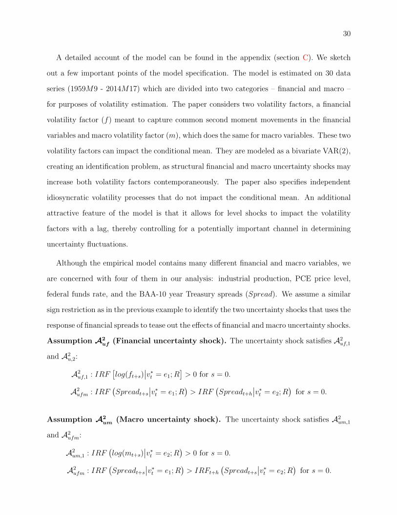
A detailed account of the model can be found in the appendix (section C). We sketch

out a few important points of the model specification. The model is estimated on 30 data

series (1959M9 - 2014M17) which are divided into two categories – financial and macro –

for purposes of volatility estimation. The paper considers two volatility factors, a financial

volatility factor (f) meant to capture common second moment movements in the financial

variables and macro volatility factor (m), which does the same for macro variables. These two

volatility factors can impact the conditional mean. They are modeled as a bivariate VAR(2),

creating an identification problem, as structural financial and macro uncertainty shocks may

increase both volatility factors contemporaneously. The paper also specifies independent

idiosyncratic volatility processes that do not impact the conditional mean. An additional

attractive feature of the model is that it allows for level shocks to impact the volatility

factors with a lag, thereby controlling for a potentially important channel in determining

uncertainty fluctuations.

Although the empirical model contains many different financial and macro variables, we

are concerned with four of them in our analysis: industrial production, PCE price level,

federal funds rate, and the BAA-10 year Treasury spreads (Spread). We assume a similar

sign restriction as in the previous example to identify the two uncertainty shocks that uses the

response of financial spreads to tease out the effects of financial and macro uncertainty shocks.

Assumption A2uf (Financial uncertainty shock). The uncertainty shock satisfies A2

uf,1

and A2u,2:

A2uf,1 : IRF

[log(ft+s)

∣∣v∗t = e1;R]> 0 for s = 0.

A2ufm : IRF

(Spreadt+s

∣∣v∗t = e1;R)> IRF

(Spreadt+h

∣∣v∗t = e2;R)

for s = 0.

Assumption A2um (Macro uncertainty shock). The uncertainty shock satisfies A2

um,1

and A2ufm:

A2um,1 : IRF

(log(mt+s)

∣∣v∗t = e2;R)> 0 for s = 0.

A2ufm : IRF

(Spreadt+s

∣∣v∗t = e1;R)> IRFt+h

(Spreadt+s

∣∣v∗t = e2;R)

for s = 0.

31

In words, the financial uncertainty shock is assumed to increase the financial volatility factor

contemporaneously while the macro uncertainty shock leads to an increase in the macro

volatility factor contemporaneously. As the assumed factor structure already specifies a

division between financial and macro volatility, we believe it reasonable to only impose that

a financial uncertainty shock increases financial volatility and a macro uncertainty shock

increases macro uncertainty. We also assume that the financial uncertainty shock leads to

a larger increase in the BAA-10 year Treasury spreads compared to the macro uncertainty

shock.

Posterior results Figure 3 shows the effects of financial (top row) and macro (bottom

row) uncertainty shocks on the economy. We use 500 parameter draws selected evenly from

the final 5, 000 parameter draws of Carriero et al. (2017a) to construct our prior robust sign

restrictions. For each parameter draw, we draw 10, 000 rotation matrices from the Haar

distribution to construct the maximum and minimum of the set.

There is evidence at the 70% prior robust credible set level that industrial production

decreases following a financial uncertainty shock. As expected, this credible region is quite

wide with such a loose sign restriction. The posterior mean bounds range from −0.74% to

−0.25% (70% set from −0.99% to −0.05%) by 3 years out. Similar to the results using the

small model, we find evidence that financial uncertainty shocks lead to long-lived declines in

industrial production.

Interestingly, the large volatility model identifies a decline in the federal funds rate follow-

ing a financial uncertainty shock at the 70% credible set level. The posterior mean bounds

of the decline is between −0.23% and −0.07% after 3 years, but prior robust credible set

suggests that the decline could be as large as 30 basis points 3 years after the financial un-

certainty shock. Therefore, the larger volatility model reinforces the weak evidence from the

small model of a decline in the federal funds rate after the financial uncertainty shock. This

result makes sense in light of the recent evidence provided by Caldara and Herbst (2016),

who find evidence of monetary policy responding to changing credit conditions. Therefore,

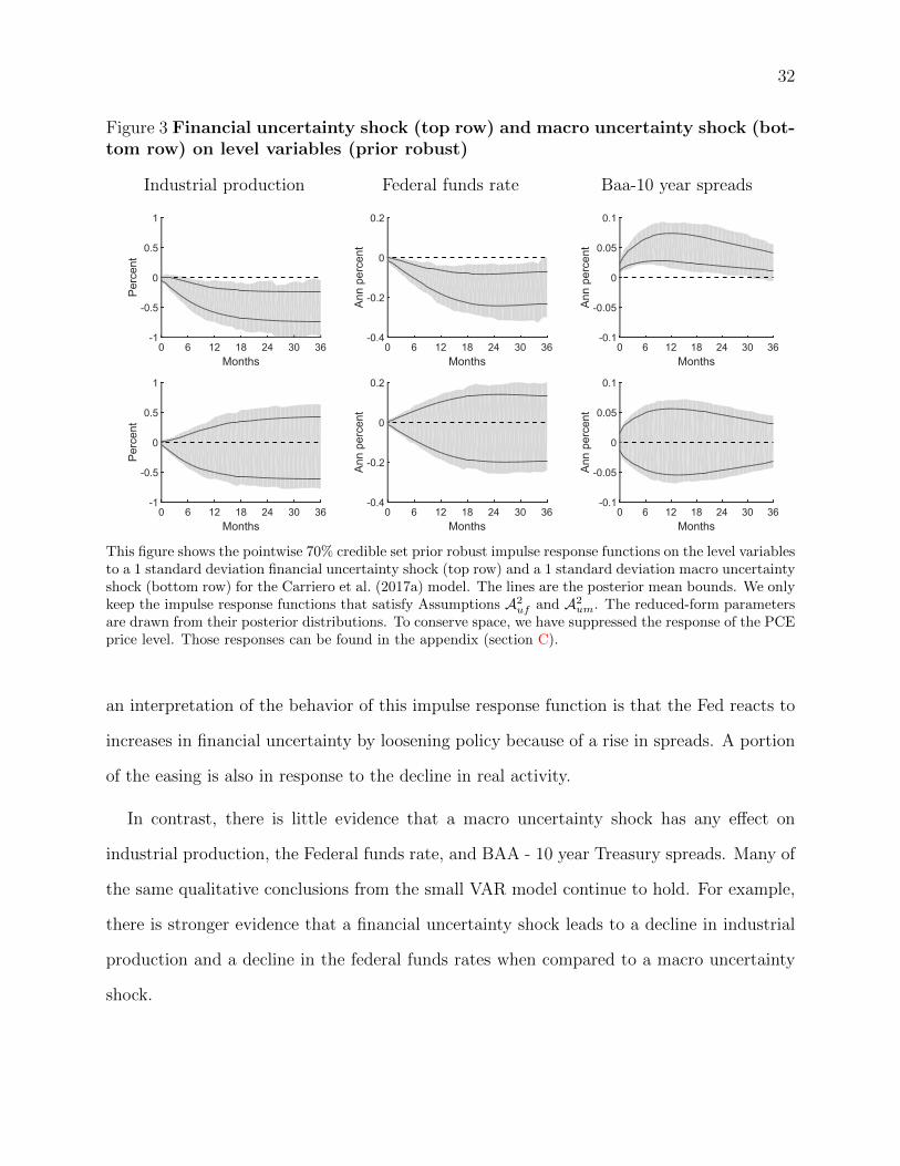
32

Figure 3 Financial uncertainty shock (top row) and macro uncertainty shock (bot-tom row) on level variables (prior robust)

Industrial production

0 6 12 18 24 30 36Months

-1

-0.5

0

0.5

1

Percent

0 6 12 18 24 30 36Months

-1

-0.5

0

0.5

1

Percent

Federal funds rate

0 6 12 18 24 30 36Months

-0.4

-0.2

0

0.2

Ann

perc

ent

0 6 12 18 24 30 36Months

-0.4

-0.2

0

0.2

Ann

perc

ent

Baa-10 year spreads

0 6 12 18 24 30 36Months

-0.1

-0.05

0

0.05

0.1

Ann

perc

ent

0 6 12 18 24 30 36Months

-0.1

-0.05

0

0.05

0.1

Ann

perc

ent

This figure shows the pointwise 70% credible set prior robust impulse response functions on the level variablesto a 1 standard deviation financial uncertainty shock (top row) and a 1 standard deviation macro uncertaintyshock (bottom row) for the Carriero et al. (2017a) model. The lines are the posterior mean bounds. We onlykeep the impulse response functions that satisfy Assumptions A2

uf and A2um. The reduced-form parameters

are drawn from their posterior distributions. To conserve space, we have suppressed the response of the PCEprice level. Those responses can be found in the appendix (section C).

an interpretation of the behavior of this impulse response function is that the Fed reacts to

increases in financial uncertainty by loosening policy because of a rise in spreads. A portion

of the easing is also in response to the decline in real activity.

In contrast, there is little evidence that a macro uncertainty shock has any effect on

industrial production, the Federal funds rate, and BAA - 10 year Treasury spreads. Many of

the same qualitative conclusions from the small VAR model continue to hold. For example,

there is stronger evidence that a financial uncertainty shock leads to a decline in industrial

production and a decline in the federal funds rates when compared to a macro uncertainty

shock.

33

6 Conclusion and Future direction

We present the sign restrictions methodology as a new approach to identifying the real

effects of uncertainty shocks. The methodology is applicable to a wide range of VAR models

with volatility-in-mean. We apply these sign restrictions on the conditional first and second

moment responses following uncertainty shocks. We investigate the real effects of financial

and macro uncertainty shocks, and find more evidence supporting that financial uncertainty

shocks lead to a decline in the macroeconomy and an easing of monetary policy. Future

work could include extending the framework to allow for a more general relationship between

contemporaneous first and second moment shocks.

References

Amir-Ahmadi, P. and T. Drautzburg (2017): “Identification through Heterogeneity,”Tech. rep.

Arias, J., J. F. Rubio-Ramırez, and D. F. Waggoner (2014): “Inference Based onSVARs Identified with Sign and Zero Restrictions: Theory and Applications,” .

Bachmann, R., S. Elstner, and E. Sims (2013): “Uncertainty and Economic Activity:Evidence from Business Survey Data,” American Economic Journal: Macroeconomics, 5,217–249.

Baker, S., N. Bloom, and S. Davis (2013): “Measuring Economic Policy Uncertainty,”Tech. rep., policyuncertainty.com.

Basu, S. and B. Bundick (2015): “Uncertainty Shocks in a Model of Effective Demand,”Boston College Working Papers in Economics 774, Boston College Department of Eco-nomics.

Baumeister, C. and J. D. Hamilton (2015): “Sign Restrictions, Structural VectorAutoregressions, and Useful Prior Information,” Econometrica, 83, 1963–1999.

Bloom, N. (2009): “The Impact of Uncertainty Shocks,” Econometrica, 77, 623–685.

Born, B. and J. Pfeifer (2014): “Policy Risk and the Business Cycle,” Journal ofMonetary Economics, 68, 68–85.

Caldara, D., C. Fuentes-Albero, S. Gilchrist, and E. Zakrajsek (2016): “TheMacroeconomic Impact of Financial and Uncertainty Shocks,” European Economic Review,forthcoming.

Caldara, D. and E. Herbst (2016): “Monetary Policy, Real Activity, and CreditSpreads: Evidence from Bayesian Proxy SVARs,” Finance and economics discussion seriesworking paper, Federal Reserve Board.

34

Canova, F. and G. D. Nicolo (2002): “Monetary disturbances matter for businessfluctuations in the G-7,” Journal of Monetary Economics, 49, 1131 – 1159.

Carriero, A., T. Clark, and M. Marcellino (2017a): “Measuring Uncertainty andIts Impact on the Economy,” Review of Economics and Statistics.

Carriero, A., T. E. Clark, and M. Marcellino (2017b): “Endogenous Uncertainty?”Working paper.

Carriero, A., H. Mumtaz, K. Theodoridis, and A. Theophilopoulou (2015):“The Impact of Uncertainty Shocks under Measurement Error. A Proxy SVAR approach,”Journal of Money, Credit and Banking.

Cogley, T. and T. J. Sargent (2005): “Drift and Volatilities: Monetary Policies andOutcomes in the Post WWII U.S,” Review of Economic Dynamics, 8, 262–302.

Creal, D. D. and J. C. Wu (2017): “Monetary Policy Uncertainty and Economic Fluc-tuations,” Tech. Rep. 4.

Faust, J. (1998): “The robustness of identified VAR conclusions about money,” Carnegie-Rochester Conference Series on Public Policy, 49, 207 – 244.

Fernandez-Villaverde, J., P. Guerron-Quintana, K. Kuester, and J. Rubio-Ramirez (2015): “Fiscal Volatility Shocks and Economic Activity,” Tech. Rep. 11.

Fernandez-Villaverde, J., P. Guerron-Quintana, J. F. Rubio-Ramirez, andM. Uribe (2011): “Risk Matters: The Real Effects of Volatility Shocks,” AmericanEconomic Review, 101, 2530–61.

Fox, E. B. and M. West (2013): “Autoregressive Models for Variance Matrices: Station-ary Inverse Wishart Processes,” Tech. rep.

Giacomini, R. and T. Kitagawa (2015): “Inference for VARs Identified with Sign Re-strictions,” Tech. rep.

Gilchrist, S. and E. Zakrajsek (2012): “Credit Spreads and Business Cycle Fluctua-tions,” American Economic Review, 102, 1692–1720.

Golosnoy, V., B. Gribisch, and R. Liesenfeld (2012): “The Conditional Autoregres-sive Wishart Model for Multivariate Stock Market Volatility,” Journal of Econometrics,167, 211–223.

Gourieroux, C., J. Jasiak, and R. Sufana (2009): “The Wishart Autoregressiveprocess of multivariate stochastic volatility,” Journal of Econometrics, 150, 167–181.

Jo, S. (2014): “The Effects of Oil Price Uncertainty on Global Real Economic Activity,”Journal of Money, Credit and Banking, 46, 1113–1135.

Jurado, K., S. C. Ludvigson, and S. Ng (2015): “Measuring Uncertainty,” AmericanEconomic Review, 105, 1177–1216.

35

Karapanagiotidis, P. (2012): “Improving Bayesian VAR Density Forecasts through Au-toregressive Wishart Stochastic Volatility,” MPRA Paper 38885, University Library ofMunich, Germany.

Leduc, S. and Z. Liu (2012): “Uncertainty Shocks Are Aggregate Demand Shocks,”Working Paper Series 2012-10, Federal Reserve Bank of San Francisco.

Ludvigson, S. C., S. Ma, and S. Ng (2015): “Uncertainty and Business Cycles: Exoge-nous Impulse or Endogenous Response?” NBER Working Papers 21803, National Bureauof Economic Research, Inc.

Moon, H. R., F. Schorfheide, and E. Granziera (2017): “Inference for VARs Iden-tified with Sign Restrictions,” Tech. rep.

Mumtaz, H. and K. Theodoridis (2016): “The Changing Transmission of UncertaintyShocks in the US: An Empirical Analysis,” Journal of Business & Economic Statistics,forthcoming.

Mumtaz, H. and F. Zanetti (2013): “The Impact of the Volatility of Monetary PolicyShocks,” Journal of Money, Credit and Banking, 45, 535–558.

Philipov, A. and M. E. Glickman (2006): “Multivariate Stochastic Volatility viaWishart Processes,” Journal of Business & Economic Statistics, 24, 313–328.

Poirier, D. J. (1998): “Revising Beliefs in Nonidentified Models,” Econometric Theory,14, 483–509.

Primiceri, G. E. (2005): “Time Varying Structural Vector Autoregressions and MonetaryPolicy,” Review of Economic Studies, 72, 821–852.

Rondina, F. (2012): “Time Varying SVARs, parameter histories, and the changing impactof oil prices on the US economy,” .

Schorfheide, F., D. Song, and A. Yaron (2016): “Identifying Long-Run Risks: ABayesian Mixed-Frequency Approach,” Tech. rep., University of Pennsylvania.

Scotti, C. (2013): “Surprise and Uncertainty Indexes: Real-Time Aggregation of Real-Activity Macro Surprises,” International Finance Discussion Papers 1093, Board of Gov-ernors of the Federal Reserve System (U.S.).

Uhlig, H. (2005): “What Are the Effects of Monetary Policy on Output? Results from AnAgnostic Identification Procedure,” Journal of Monetary Economics, 52, 381–419.