mathematics

Article

A New Ant Colony-Based Methodology forDisaster Relief

José M. Ferrer 1,* , M. Teresa Ortuño 2 and Gregorio Tirado 1

1 Department of Financial and Actuarial Economics & Statistics, Interdisciplinary Mathematics Institute,Complutense University of Madrid, HUMLOG Research Group, 28040 Madrid, Spain; gregoriotd@ucm.es

2 Department of Statistics and Operational Research, Interdisciplinary Mathematics Institute, ComplutenseUniversity of Madrid, HUMLOG Research Group, 28040 Madrid, Spain; mteresa@ucm.es

* Correspondence: jmferrer@ucm.es

Received: 2 March 2020; Accepted: 27 March 2020; Published: 3 April 2020�����������������

Abstract: Humanitarian logistics in response to large scale disasters entails decisions that mustbe taken urgently and under high uncertainty. In addition, the scarcity of available resourcessometimes causes the involved organizations to suffer assaults while transporting the humanitarianaid. This paper addresses the last mile distribution problem that arises in such an insecureenvironment, in which vehicles are often forced to travel together forming convoys for securityreasons. We develop an elaborated methodology based on Ant Colony Optimization that is appliedto two case studies built from real disasters, namely the 2010 Haiti earthquake and the 2005 Nigerfamine. There are very few works in the literature dealing with problems in this context, and that isthe research gap this paper tries to fill. Furthermore, the consideration of multiple criteria such ascost, time, equity, reliability, security or priority, is also an important contribution to the literature,in addition to the use of specialized ants and effective pheromones that are novel elements of thealgorithm which could be exported to other similar problems. Computational results illustrate theefficiency of the new methodology, confirming it could be a good basis for a decision support tool forreal operations.

Keywords: Ant Colony Optimization; humanitarian logistics; last mile distribution; disaster relief

1. Introduction

Disaster management remains a crucial challenge for the international community. National andsupranational institutions and non-governmental organizations have to deal with high impact disasterssuch as the 2010 Haiti earthquake, the 2013 Typhoon Haiyan or the 2018 Sulawesi earthquake andtsunami. This global concern is reflected in the scientific literature and specifically in the OperationsResearch community, where the increasing interest on humanitarian logistics and disaster managemententails the publication of surveys [1,2], books [3,4], special issues [5,6] and journals (such as the Journalof Humanitarian Logistics and Supply Chain Management).

Within the disaster management cycle, the response phase includes the actions to be performedonce the disaster has occurred. Research on the response phase may focus on specific types of disasters,such as earthquakes [7,8] or floods [9], or can address particular problems for generic disasters, such aslocation-allocation [10], evacuation [11], or debris management [12]. Among the operations to becarried out after a disaster strikes, the distribution of aid to the affected people plays an important role.Along with the usual objectives in commercial logistics, mainly the operation cost, in humanitarianlogistics other attributes have to be considered [13,14], such as the response time, the equity of thedistribution, etc. Therefore, multi-criteria models are necessary to face many realistic problems in this

Mathematics 2020, 8, 518; doi:10.3390/math8040518 www.mdpi.com/journal/mathematics

Mathematics 2020, 8, 518 2 of 23

context. Gutjahr and Nolz [15] provide a review on multi-criteria decision making in humanitarian aidclassifying the existing models as deterministic or stochastic and pre-disaster or post-disaster.

Many times the distribution operations must be performed under unsecure conditions [6].Assaults to relief vehicles are sadly frequent and this complicates the work of organizations thatexecute the aid missions. Avoiding as much as possible the most dangerous roads and forcing thevehicles to travel together forming convoys are two ways of improving the security of the operations.

In this paper, we develop an algorithm based on Ant Colony Optimization (ACO) metaheuristicto solve the multi-criteria last mile distribution problem in an unsecure environment stated in [16].The complexity of this problem makes it necessary to use a heuristic approach to solve realisticcases. Besides, due to the strong links between the elements of a solution, it is difficult to developheuristics that perform progressive alterations of a solution while ensuring feasibility, as it is the caseof evolutionary algorithms or local search heuristics. Instead, algorithms based on constructionof solutions, such as Greedy Randomized Adaptive Search Algorithm (GRASP) or Ant ColonyOptimization metaheuristics, fit much better.

The ACO methodology that we propose in this work presents some novelties that make it suitablefor routing and distribution problems in which the vehicles must travel in convoys. The use of convoysis appropriate not only in humanitarian operations, but in any logistics operation performed in anenvironment of insecurity, in which attacks on delivery vehicles to steal the commodities are possible.The algorithm considers two types of ants—vehicles and aid kits—four types of standard pheromones,and especially the use of effective pheromones, updatable in the course of each solution buildingprocess. This new concept allows a better balance between the elements of a solution and a higherdiversification in the set of solutions that can be built. Effective pheromones may be applied to awide variety of problems, especially vehicle routing problems involving a large number of vehicles.The results obtained show that the new ACO Algorithm proposed in this paper is a useful decisionaid tool. The ACO Algorithm provides good quality solutions in a short time in realistic test cases,frequently improving the solutions obtained with the GRASP Algorithm developed in [16].

The rest of this paper is organized as follows. Section 2 reviews the relevant literature onmulti-criteria optimization for the last mile distribution problem, as well as some applications of AntColony Optimization in disaster management. Section 3 presents the problem of transportation forlast mile distribution, including the data notation and the description of the six attributes considered.Section 4 introduces the heuristic method proposed to solve the problem. An Ant Colony Optimizationalgorithm is developed together with the subordinate procedure that guides the construction of feasiblesolutions. Section 5 is devoted to showing and analyzing the results obtained when applying theproposed metaheuristic to solve two test cases based on real disasters. Finally, Section 6 draws someconclusions derived from this work.

2. Literature Review

Some of the most significant papers that apply multi-criteria techniques in humanitarian lastmile distribution are mentioned below and summarized in Table 1. Viswanath and Peeta [8] developa multicommodity mixed integer programming model in order to maximize the total populationcovered and minimize the total travel time for earthquake response. Balcik et al. [17] present amulticommodity, multimodal and multiperiod last mile distribution problem and establish a scalarobjective function that aggregates minimization of transportation costs and maximization of demandcovered. Nolz et al. [18] consider three attributes (reliability of the transporting tours, coverage andtotal travel time) in a distribution problem where infrastructure may be damaged in a post-disastersituation. Lin et al. [19] use the scalarization approach to deal with a three-objective (total unsatisfieddemand, total travel time and equity of the distribution) integer programming model that allowssplit deliveries. Two heuristic methods are proposed to solve the model. Bozorgi-Amiri et al. [20]propose a robust stochastic compromise programming model for disaster relief logistics, minimizingthe sum of the expected value and the variance of the total cost and minimizing the sum of the

Mathematics 2020, 8, 518 3 of 23

maximum unsatisfied demands. Tirado et al. [21] consider four attributes (amount of aid distributed,time of the operation, equity and cost) in a dynamic flow model that is solved via lexicographical goalprogramming. Huang et al. [22] develop a quadratic multi-objective programming model to face anallocation and distribution problem. Three attributes are considered: lifesaving utility, delay cost andequity of the distribution. This model allows vehicles to visit a node more than once and provides theindividual itineraries of the vehicles. Ahmadi et al. [23] aggregate the distribution time, the penaltycost of unsatisfied demand and the costs of opening distribution centers into a single objective functionfor a location-routing problem considering network failure, random travel times and multiple usesof vehicles. Zhou et al. [24] apply a multi-objective evolutionary algorithm to solve a multiperiodand multicommodity distribution model which aims to minimize the unsatisfied demand and tominimize the risk of choosing damaged roads. Maghfiroh and Hanaoka [25] present a multimodalmodel considering dynamic and stochastic demands in order to minimize the travel time and theunmet demand. Moreno et al. [26] develop a biobjective multiperiod stochastic location-transportationmodel that allows multiple trips to the vehicles not only in different periods, but also in the sameperiod. The authors propose different heuristic techniques to solve the model. Outside the scopeof aid distribution, Habib et al. [27] address a post-disaster waste management problem through apossibilistic programming model that minimizes both the cost of waste processing and the carbonemissions and maximizes the job opportunities.

Despite the frequency with which aid distribution is to be carried out in unsafe conditions,only a few papers consider the security as an attribute. Ortuño et al. [28] integrate seven attributes(quantity distributed, time of response, cost, equity, priority, reliability and security) into a linearlexicographical goal programming flow model. This model is multimodal, multidepot, allows splitdeliveries and vehicles travel in convoys so that they can be escorted. An alternative version of thismodel is established in Vitoriano et al. [29], where the authors set a fixed amount to distribute andcombine the six remaining attributes into a non-lexicographical model. Nevertheless, these models donot provide the individual route of each vehicle, so it is not possible to easily implement plans for therelief distribution. Ferrer et al. [16] propose a GRASP metaheuristic to solve a nonlinear multi-objectivemodel that allows vehicles to visit a node more than once and provides the individual itineraries ofthe vehicles. The mathematical formulation of this model is established in Ferrer et al. [30], where anextensive comparison of the characteristics of the models is made with other studies that deal with thelast mile distribution problem.

Table 1. The literature related to multi-criteria techniques in humanitarian last mile distribution.

Reference # Criteria Security Multi-Criteria Approach Heuristic Approach

Ahmadi et al. [23] 3 Scalarization Variable Neighborhood SearchBalcik et al. [17] 2 Scalarization -Bozorgi-Amiri et al. [20] 2 Compromise Programming -Ferrer et al. [16] 6 X Compromise Programming GRASPHabib et al. [27] 3 Interactive Method -Huang et al. [22] 3 Scalarization -

Lin et al. [19] 3 Scalarization Genetic Algorithm,ad-hoc heuristic

Maghfiroh and Hanaoka [25] 2 Scalarization -

Moreno et al. [26] 2 Hierarchical Optimization, Fix and Optimize,Scalarization ad-hoc heuristic

Nolz et al. [18] 3 Pareto Optimization Memetic Algorithm,ad-hoc heuristic

Ortuño et al. [28] 7 X Goal Programming -Tirado et al. [21] 3 Goal Programming -Viswanath and Peeta [8] 2 Pareto Optimization -Vitoriano et al. [29] 6 X Goal Programming -Zhou et al. [24] 2 Pareto Optimization Evolutionary AlgorithmThis study 6 X Compromise Programming Ant Colony Optimization

Mathematics 2020, 8, 518 4 of 23

In this study, we propose an Ant Colony Optimization methodology to solve the model developedin [16] and [30]. Even though ACO has been applied frequently to different routing and distributionproblems [31–34], it has barely been used in the context of disaster management. The most remarkablework is Yi and Kumar [35], where the authors apply this metaheuristic to solve a distribution andevacuation problem. More recently, Saeidian et al. [36] combine different techniques, including ACO,to face a location-allocation problem of relief centers after an earthquake. Therefore, this paperpresents the first application of Ant Colony Optimization to a multi-criteria last mile distributionproblem. Furthermore, the proposed ACO methodology introduces novelties such as specializedants, representing both vehicles and aid kits, and effective pheromones, that conveniently balance theelements of the built solutions.

3. Problem Description

The last mile distribution problem addressed in this paper consists in deciding how to dealout a predetermined amount of humanitarian aid from distribution centers to populations in needby moving a set of vehicles through a transportation network. We consider that the distribution isperformed in an insecure and uncertain environment and, as a consequence, the convoys transportingthe aid may be attacked while traveling and some roads may be unavailable due to damages producedby the disaster.

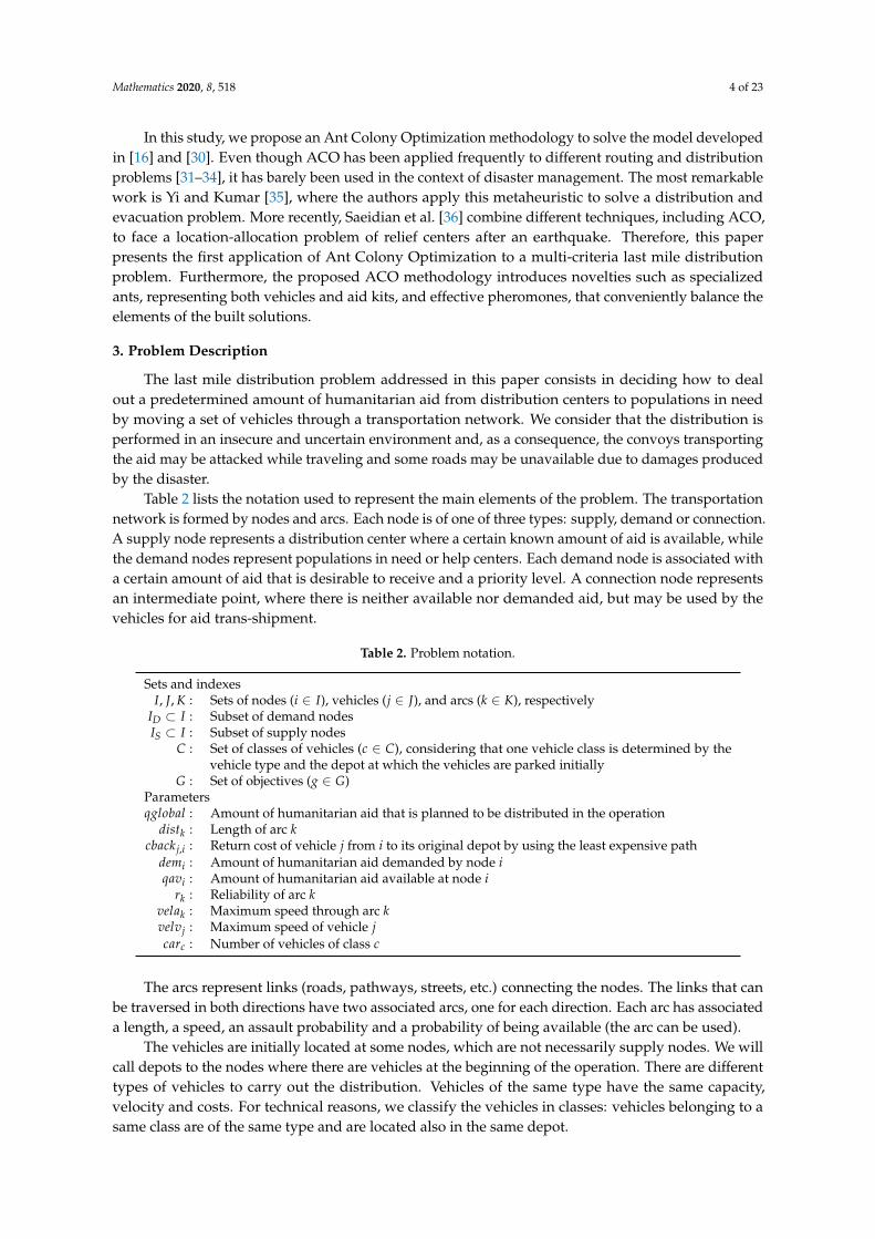
Table 2 lists the notation used to represent the main elements of the problem. The transportationnetwork is formed by nodes and arcs. Each node is of one of three types: supply, demand or connection.A supply node represents a distribution center where a certain known amount of aid is available, whilethe demand nodes represent populations in need or help centers. Each demand node is associated witha certain amount of aid that is desirable to receive and a priority level. A connection node representsan intermediate point, where there is neither available nor demanded aid, but may be used by thevehicles for aid trans-shipment.

Table 2. Problem notation.

Sets and indexesI, J, K : Sets of nodes (i ∈ I), vehicles (j ∈ J), and arcs (k ∈ K), respectively

ID ⊂ I : Subset of demand nodesIS ⊂ I : Subset of supply nodes

C : Set of classes of vehicles (c ∈ C), considering that one vehicle class is determined by thevehicle type and the depot at which the vehicles are parked initially

G : Set of objectives (g ∈ G)Parametersqglobal : Amount of humanitarian aid that is planned to be distributed in the operation

distk : Length of arc kcbackj,i : Return cost of vehicle j from i to its original depot by using the least expensive path

demi : Amount of humanitarian aid demanded by node iqavi : Amount of humanitarian aid available at node i

rk : Reliability of arc kvelak : Maximum speed through arc kvelvj : Maximum speed of vehicle jcarc : Number of vehicles of class c

The arcs represent links (roads, pathways, streets, etc.) connecting the nodes. The links that canbe traversed in both directions have two associated arcs, one for each direction. Each arc has associateda length, a speed, an assault probability and a probability of being available (the arc can be used).

The vehicles are initially located at some nodes, which are not necessarily supply nodes. We willcall depots to the nodes where there are vehicles at the beginning of the operation. There are differenttypes of vehicles to carry out the distribution. Vehicles of the same type have the same capacity,velocity and costs. For technical reasons, we classify the vehicles in classes: vehicles belonging to asame class are of the same type and are located also in the same depot.

Mathematics 2020, 8, 518 5 of 23

The humanitarian aid is packed in kits composed of water, food, medicines, blankets, etc.The operation to be performed consists of delivering qglobal of such kits.

In addition, the design of the routes must be carried out under the following assumptions:

− Vehicles can visit a node more than once. Likewise, they can pick up or deliver humanitarian aidmore than once, even in the same node.

− Transhipment of aid between vehicles can be made at any node.− Split pick up and delivery are allowed in all supply and demand nodes, respectively.− For security reasons, all vehicles traveling through an arc must do it together forming a convoy.

In this way, the convoys can be escorted. As a result, each vehicle can pass through an arcjust once.

− The probability of assault to a convoy decreases with the size of the convoy.− Vehicles must return to their respective depots at the end of the operation. The return of each

vehicle will be made through the least expensive path, being cback j,i the return cost of vehicle j tonode i. Assaults on return itineraries are not considered.

− In the last trip of its route (before it returns), each vehicle must transport some aid. This isimposed to prevent trips of empty vehicles with the only purpose of increasing convoy safety.

As usual in humanitarian logistics, this problem is intrinsically multi-criteria. In this case,we consider six different attributes that will be incorporated into the model as objectives to beminimized. In what follows, a description of the attribute measures used in the model is provided;however, since they are not necessary for the understanding of the paper, we decided to omit themathematical formulation. The interested reader can see [16] for further details.

Time. The distribution is done in an emergency situation, so we consider the time of theoperation as an attribute. The operation finishes when the last kit of aid is delivered toa demand point, the return times are not considered.

Cost. The total cost of the operation, including fixed and variable costs and the return costs,is also an attribute. In many cases, there may be a budget that can not be exceeded.

Equity. Since the available aid or the amount of aid planned to distribute are usually lowerthan the total demanded aid, very frequently it is not possible to fully meet the demand.Thus, it is necessary to consider the equity of the distribution as an attribute. In aperfectly fair deal all demand nodes must receive aid in the same proportion, that willbe called ideal demand proportion, as established in (1).

idp =qglobal

∑i∈IDdemi

(1)

The equity measure is defined as the square root of the quadratic deviation ofthe proportions of satisfied demand from the ideal demand proportion over alldemand nodes.

Priority. The priority attribute is measured by the sum of relative unsatisfied demands over alldemand nodes weighted by their priority levels. The priority levels are considered fortwo reasons. On the one hand, a higher level of priority may indicate greater urgencyin the demand node. On the other hand, there can be nodes that, due to having difficultaccess or belonging to insecure or damaged areas, are not visited at all. Then, a highpriority level is required for such nodes.

Security. Dealing with an insecure environment is a main feature of the problem we areconsidering. In addition to the probabilities of assault to the convoys, how severean assault is must also be taken into account. For this purpose, we use an elaboratedmeasure that evaluates the expected gravity of suffering attacks due to the amount ofaid that would be lost.

Mathematics 2020, 8, 518 6 of 23

Reliability. As in the security attribute, not only the availability of the arcs must be considered,but also the consequences of finding not passable arcs. Thus, the reliability measureevaluates the expected aid loss over all arcs.

The objectives can be minimized separately or in an aggregated function as in (2), where weightswg, g ∈ G represent the preferences of the decision maker and fg is the objective function associatedwith the attribute g.

f = ∑g∈G

wg fg (2)

For obtaining solutions that take all attributes into account in a balanced way, we applycompromise programming (CP), introduced in Cochrane and Zeleny [37]. CP is a multi-criteria decisionmaking technique which consists in minimizing the distance to the ideal point. The components of theideal point are the optimal values of the attributes when optimized independently. To normalize theattributes, the difference between the ideal and the anti-ideal is used, where the components of theanti-ideal point are the worst values for the attributes on the set of non-dominated solutions.

The CP objective function when using the p-norm is denoted as f̃p and defined as follows:

f̃p =

[∑

g∈Gwg

(fg − i+gi−g − i+g

)p] 1p

(3)

Again, wg, g ∈ G represent the preferences of the decision maker, while i+g and i−g are the idealand the anti-ideal components associated with attribute g, respectively.

4. Heuristic Approach

In this section we present an algorithm based on Ant Colony Optimization, that was introducedin Dorigo et al. [38]. The ACO metaheuristic emulates the way in which the ants of a colony manage tofind the shortest path from the anthill to a source of food through the pheromone trails deposited by theants when they move. Extensive information about ACO metaheuristic and its multiple variants can befound in [39–41]. The metaheuristic algorithm that we propose in this paper takes some elements of theAnt Colony System (ACS) developed in Dorigo and Gambardella [42] to establish a multiple-ant colonysystem variant. Section 4.1 is devoted to the main program of the metaheuristic (ACO Algorithm),and Section 4.2 to the subordinate procedure that performs the construction of solutions (PheromoneTrail Constructive Algorithm or PTC Algorithm).

Table 3 shows the main parameters and variables that are used in the metaheuristic. According tothe ACS, two types of pheromone updates are made. The global update is performed every time mconsecutive solutions are obtained and is intended to improve the construction of future solutions.The local update is performed after each single solution is obtained, and its purpose is to diversify theconstruction. Parameters ρg and ρl are the corresponding evaporation rates. Our algorithm uses twotypes of ants, representing vehicles and humanitarian aid kits, and four types of pheromones, that aredeposited by the vehicles or by the aid kits in different situations. First type (respectively secondtype) pheromones are deposited by the vehicles (aid kits) when moving through the arcs, third typepheromones are associated with the amounts of aid leaving supply nodes, and fourth type pheromonescorrespond to the amounts of aid remaining at the nodes at the end of the operation. τ1

c,k, τ2k , τ3

i and τ4i

are the variables that indicate the quantities of pheromone of the four types that have been depositedat an arc k or at a node i.

The construction of solutions takes into account both pheromones and visibility. Pheromonesindicate how often each element candidate to be added to the current partial solution was selected byprevious ants, while visibility, established as greedy functions, indicates how good an element couldbe according to each of the objectives considered.

Mathematics 2020, 8, 518 7 of 23

The PTC Algorithm builds new solutions by adding elements iteratively. As a result, the valuesof the pheromones associated with the added elements should be decreased to prevent an excessiveconcentration of these elements in the solution. This is achieved through what we called effectivepheromones, a new concept that refers to variables that at the beginning of the execution of the PTCAlgorithm take the same values as the corresponding pheromones variables, but which will be updatedduring the construction of the solution.

Table 3. Heuristic approach notation.

Parametersρl : Local evaporation rateρg : Global evaporation rateσ1 : Greedy functions weight at the beginning of the algorithmσ2 : Growth rate of pheromones weightm : Number of solutions obtained between two consecutive global updatesq0 : Probability of choosing the element with the highest score in any of the decision situationsn : Total number of solutions to be obtained

Variablesλ : Variable that controls pheromones weight versus greedy functions weight

τ1c,k : First type pheromone in arc k for the vehicles of class cτ2

k : Second type pheromone in arc kτ3

i : Third type pheromone in supply node i ∈ IOτ4

i : Fourth type pheromone in node i ∈ ID ∪ IO$

gζ : Individual greedy function of objective g associated to element ζ

f si : Final stock at node i in the current solutionltk : Amount of aid transported by arc k in the current solution

vtc,k : Number of vehicles of class c traversing arc k in the current solution

4.1. Ant Colony Optimization Algorithm

In this subsection we introduce the ACO Algorithm, whose pseudocode is given in Algorithm 1.Its main steps are explained below.

Algorithm 1 ACO algorithm

1: Perform preprocess.2: Create a solution S∗ with the PTC Algorithm.3: for it = 2, · · · , n do

4: Create a new solution S with the PTC Algorithm.5: if S is better than S∗ then

6: Do S∗ = S.7: end if8: Perform the local update.9: if it ≡ 0 (mod m) then

10: Perform the global update.11: end if12: Increase λ.13: end for14: Output S∗.

Preprocess. It comprises several tasks needed before starting the construction of solutions:

• Simplify the logistic network removing unnecessary arcs.• For each vehicle, calculate the least expensive return paths from any node to its depot via

Dijkstra’s algorithm→ cback j,i.

Mathematics 2020, 8, 518 8 of 23

• Calculate bounds for the greedy functions→ bg.• Initialize λ and pheromones.

Pheromone update. The local update increases the pheromones of the elements that appear lessfrequently in the previous iteration in order to diversify the construction, as stated in Equations(4)–(7).

τ1c,k = (1− ρl)τ

1c,k +

ρl1 + vtc,k

∀c, ∀k (4)

τ2k = (1− ρl)τ

2k +

ρl1 + ltk

∀k (5)

τ3i = (1− ρl)τ

3i +

ρl1 + qavi − f si

∀i ∈ IS (6)

τ4i = (1− ρl)τ

4i +

ρl1 + f si

∀i ∈ ID ∪ IS (7)

In the same way, the global update increases the pheromones of the elements that appear morein the current best known solution in order to guide the construction towards potentially bettersolutions, as stated in Equations (8)–(11). The auxiliary parameter clc in (8) denotes the numberof vehicles of class c, while the asterisk in vt∗c,k, lt∗k and f s∗i indicates that these auxiliary variablescorrespond to the current best known solution.

τ1c,k = (1− ρg)τ

1c,k +

vt∗c,k

clc∀c, ∀k (8)

τ2k = (1− ρg)τ

2k +

lt∗kqglobal

∀k (9)

τ3i = (1− ρg)τ

3i +

qavi − f s∗iqavi

∀i ∈ IS (10)

τ4i =

(1− ρg)τ4i +

f s∗iqavi

∀i ∈ IS

(1− ρg)τ4i +

f s∗idemi

∀i ∈ ID(11)

The elements that are taken into account in both updates are the following: for the first typepheromones, the class-arc pairs (4) and (8); for the second type pheromones, the amounts oftransported aid in the arcs (5) and (9); for the third type pheromones, the amounts of aid that havecome out from the supply nodes (6) and (10); and for the fourth type pheromones, the amountsof aid that remain in the supply and demand nodes at the end of the distribution (7) and (11).

Increase λ. Variable λ, which controls the weight of pheromones and visibility, grows over thecourse of the ACO Algorithm so that the importance of pheromones in the construction isincreasing. The pheromones weight is updated according to (12), where it is the current iteration.The exponential expression makes the increase of λ to be progressively slower.

λ = 1− σ1e−σ2itn (12)

4.2. Pheromone Trail Constructive Algorithm

The pseudocode of PTC Algorithm is shown in Algorithm 2. Lines 1 and 2 are the constructivesteps, where pheromone and greedy functions are introduced in order to guide the solution buildingprocess. Lines 3 to 12 coordinate the elements of the current solution and determine if it is feasible.It must be taken into account that, as all vehicles travel in convoys through the arcs, the solution mustsatisfy the precedence relation induced on the set of arcs. Lines 13 to 17 intend to improve the solutionwith the help of pheromone functions.

Mathematics 2020, 8, 518 9 of 23

The solution is built iteratively by adding or removing elements, being the nature of the elementsdependent on the algorithm step. An element can be, for example, a trip of a vehicle or a demandnode where to drop an aid kit. If ζ is a candidate element to be added, phζ and grζ are, respectively,the effective pheromone and the greedy function associated to it. As a result, the score of element ζ iscalculated as stated in (13).

scζ = λphζ + (1− λ)grζ (13)

The reason why this expression is additive rather than multiplicative—as usual in ACO—isbecause, in this way, the gradual increase of the pheromone weight can be more accurately controlled.

Algorithm 2 PTC Algorithm

1: Design itineraries, form convoys and calculate arriving times at nodes.2: Deliver aid through the network.3: if all planned aid is delivered then

4: Determine arriving and departure events.5: Calculate stocks after events.6: else

7: Go back to line 1.8: end if9: Try to eliminate all negative stocks at nodes.

10: if there exists any negative stock then

11: Go back to line 1.12: end if13: Improve equity.14: Adjust supply nodes.15: Trim routes.16: Eliminate aid crossings.17: Exchange vehicles.

The greedy function of a candidate element ζ is stated in (14), where $gζ is the individual greedy

function of objective g, wg is the weight of objective g in the objective function and bg is an upperbound for $

gζ .

grζ = ∑g∈G

wg

(bg − $

gζ

bg

)(14)

The greedy functions are used only where it is possible to define them in a reasonable way.When there are no greedy functions, the score is simply scζ = phζ if the decision regards which elementshould be added to the partial solution (it is convenient to select elements with more pheromone) or asstated in (15) if the decision regards which element should be removed from the partial solution (it isconvenient to select elements with less pheromone).

scζ =1

phζ(15)

In all steps of the PTC Algorithm, the elements are chosen according to the criterion established inACS: if q ≤ q0, where q is a random variable uniformly distributed over [0, 1], the candidate elementwith the highest score is chosen; otherwise, the election is made according to the probabilities statedin (16), which are proportional to the scores.

prζ =scζ

∑ζ̃ scζ̃

(16)

Mathematics 2020, 8, 518 10 of 23

The main steps of the PTC Algorithm are described in detail in what follows.

Design itineraries. The routes to be followed by the vehicles are built iteratively, starting from anempty solution where all the vehicles are parked at their corresponding depots. At each iteration,the candidate elements to be added to the partial solution are the feasible trips of every singlevehicle j through an available arc k. Therefore, each element is a pair ζ = (j, k). The effectivepheromone associated to each element is defined in (17), where c is the vehicle class correspondingto vehicle j.

phζ=

(1−

vtc,k

carc

)τ1

c,k (17)

On the one hand, the effective pheromone is proportional to the first type pheromone, τ1c,k,

which depends on the vehicles of class c traversing arc k in the previously obtained solutions.In particular, the more vehicles of class c transit through this arc in the current best knownsolution, the more effective pheromone candidate element (j, k) has. On the other hand,the effective pheromone depends on the number of vehicles of class c traversing arc k in thecurrent partial solution, so the greater vtc,k is, the less effective pheromone candidate element(j, k) has. If this gradual adjustment of the effective pheromone is not performed, it could leadto an excess of vehicles of a class through an arc for those pairs (c, k) with higher first typepheromone. This eventual excess of elements in a solution justifies the use of the effectivepheromone and it also applies to other steps of the PTC Algorithm.

All the greedy functions used in the PTC Algorithm are defined in the same way as in the Elite SetConstructive Algorithm (ESCA) described in [16]. For example, the individual greedy functionof the time objective is the time that takes vehicle j to traverse arc k (18), while the individualgreedy function of the reliability objective is the probability that arc k is not available (19).

$tζ=

distkmin{velak, velvj}

(18)

$ fζ= 1− rk (19)

The score of each element is calculated as stated in (13). Once an element (j, k) is chosen, arc k isadded to the route of vehicle j and the associated precedence relations are updated, in order toensure that all vehicles travel together in convoys. The construction process is iterated until theroutes cannot be continued any longer.

Form convoys and calculate arriving times. The convoys are formed by all vehicles traveling througheach arc. The travel speed of a convoy is determined by the minimum between the maximumvelocity of the slowest vehicle of the convoy and the maximum speed of the associated arc.The arriving times of the convoys at their destination nodes are calculated as the minimum timesat which the convoys can finish their trips through the arcs taking into account the travel speedsand the precedence relation on the arcs.

Aid distribution. Once the itineraries of the vehicles are designed, the amount of aid transported byeach convoy must be determined. For this purpose, an auxiliary transportation network is built,including all the nodes of the original network but only the arcs traversed by convoys, accordingto the itineraries determined previously. Several dummy arcs and two dummy nodes are alsoadded: the source node (sc), linked to all supply nodes by dummy arcs, and the sink node (sn),linked to each demand node also by dummy arcs. The capacities of the dummy arcs leaving thesource or arriving at the sink are equal to the aid availability or the demand of the correspondingsupply or demand node, respectively. The capacity of each original arc is equal to the capacity of

Mathematics 2020, 8, 518 11 of 23

the convoy traversing it. The calculation of the flow of aid through this network is performed byapplying a modified version of the Ford-Fulkerson algorithm [43].

The augmenting paths from the source to the sink are determined iteratively, node by node,as follows:

• If the current node is the source, the candidate elements are the supply nodes with availableaid. The effective pheromone of each supply node, ζ = i, is stated in (20), where f lsc,i is thecurrent flow from the source to the supply node i, i.e., the amount of aid leaving the supplynode i in the current partial flow solution. The effective pheromone depends positivelyon the third type pheromone (which is related to the amount of aid leaving supply node iin the previously obtained solutions) and negatively on the amount of aid leaving i in thecurrent solution.

phζ =

(1− f lsc,i

qavi

)τ3

i (20)

No greedy function is defined in this case, so the score of each supply node i is equal to thecorresponding effective pheromone.

• If the current node is a node i0 different from the source, a candidate element is a node ilinked to i0 through an arc k = (i0, i) with positive residual capacity. The effective pheromoneof each candidate node, ζ = i, is calculated as stated in (21). It depends positively on theamount of aid transported through arc k in the previously obtained solutions and negativelyon the amount of aid transported through arc k in the current solution.

phζ =

(1−

f li0,i

qglobal

)τ2

k (21)

The individual greedy function of the time objective is the arriving time of the convoyassociated to arc k, the individual greedy function of the cost objective is the average cost oftransporting an aid kit by arc k among the vehicles of the associated convoy, etc.

If the current node i0 is a demand node, in addition to the other candidates mentioned earlier,the sink sn must be considered as a candidate element as well. The selection of the sinkwould finish the augmenting path. Its effective pheromone (22) depends positively on theamount of aid remaining at demand node i0 at the end of the operation in the previouslyobtained solutions and negatively on the remaining aid in the current solution.

phsn =

(1−

f li0,sn

demi0

)τ4

i0 (22)

The individual greedy function of the equity objective associated to the sink measureshow the deviation of the proportion of satisfied demand at node i0 from the ideal demandproportion would vary if the sink is selected; the individual greedy function of the priorityobjective is obtained in a similar way; and the individual greedy functions of the otherobjectives take the value 0, because finishing the augmenting path does not worsenthose objectives.

Finally, the scores are established according to (13).

Each time a node is selected and labeled, the current node is updated. Once an augmenting pathis determined, the flow is updated according to the Ford-Fulkerson algorithm. The process isiterated until all the planned amount of aid is distributed from the source to the sink or it is not

Mathematics 2020, 8, 518 12 of 23

possible to find an augmenting path, in which case the current solution would be discarded andthe algorithm would be restarted at Step 1.

Determine events and calculate stocks. The events in each node correspond to the arrivals anddepartures of convoys. Once the timing of the events are determined, the stocks, i.e., the amountsof aid available after each event, are obtained.

Eliminate negative stocks. At this point, some negative stock may be found because a convoy departsfrom a node transporting some aid that has not arrived yet. In order to avoid this, additionalprecedence relations forcing the arrival of aid to occur before the corresponding departure areadded when needed.

Improve equity. This step is executed if there is aid leaving a demand node in which the proportionof satisfied demand is less than the ideal demand proportion. A demand node that verifiesthis condition is called improvable node. In order to keep the maximum possible amount of aidat the improvable nodes, a variation of the maximum flow problem is solved, as in the Aiddistribution step. The auxiliary transportation network includes all the nodes but only the usedarcs. The source node is linked to all improvable nodes by dummy arcs, and the sink node islinked by dummy arcs arriving from the demand nodes in which the proportion of satisfieddemand exceeds the ideal demand proportion. The capacity of each dummy arc leaving thesource is the minimum between the amount of aid leaving that node and the residual amountof aid needed to reach the ideal demand proportion. The capacity of each dummy arc reachingthe sink is the amount of aid exceeding the ideal demand proportion at the associated node.The capacity of each original arc is equal to the amount of aid transported through it.

The augmenting paths from the source to the sink are determined in a similar way as in the Aiddistribution step:

• If the current node is the source, the candidate elements are the improvable nodes.The effective pheromone of each improvable node, ζ = i, is stated in (23). The effectivepheromone depends positively on the final stock at node i in the previously obtainedsolutions and negatively on the final stock at node i in the current solution.

phζ =

(1− f si

demi

)τ4

i (23)

The score of each improvable node i is equal to the corresponding effective pheromone.

• If the current node is a node i0 different from the source, a candidate element is a node ilinked to i0 through an arc k = (i0, i) with positive residual capacity. The effective pheromoneof each candidate node, ζ = i, is calculated as stated in (24). It depends positively on theamount of aid transported through arc k in the previously obtained solutions and negativelyon the amount of aid transported through arc k in the current solution.

phζ =

(1−

ltk − f li0,i

1 + qglobal

)τ2

k (24)

Since we are interested in removing needless flow, the score of each improvable node i isinversely proportional to the effective pheromone, as established in (15). Note that the unitadded in the denominator of the fraction in (24) prevents the effective pheromone frombeing 0.

If the current node i0 is a demand node linked to the sink, the sink must be considered asa candidate element as well. Its effective pheromone (25) depends positively on the final

Mathematics 2020, 8, 518 13 of 23

stock at demand node i0 at the end of the operation in the previously obtained solutions andnegatively on the final stock at i0 in the current solution.

phsn =

(1−

s fi01 + demi0

)τ4

i0 (25)

The score of the sink is established according to (15) as well.

Each time an augmenting path is obtained, the flow is updated according to the Ford-Fulkersonalgorithm. The final stock at each demand node i, s fi, and the amount of aid transported througheach arc k, ltk, are updated as well. The algorithm stops when the current flow cannot beincreased further.

Adjust supply nodes. The purpose of this step is to eliminate as much incoming flow of aid as possibleat supply nodes in which there is aid available at the end of the operation. Once again, a variationof the maximum flow problem is solved. The auxiliary transportation network includes allthe nodes and the used arcs, which are now reversed because we try to return flow back fromthe supply nodes. All supply nodes are linked to the source and to the sink by dummy arcs.The capacity of each dummy arc leaving the source is the minimum between the amount ofload arriving to the corresponding supply node and the final stock at it. The capacity of eachdummy arc reaching the sink is the amount of aid available initially at the corresponding supplynode. The capacity of each remaining arc is equal to the amount of aid transported through it (inopposite direction).

The calculation of the effective pheromones is as follows:

• If the current node is the source, the candidate elements are the supply nodes. The effectivepheromone of each supply node, ζ = i, is stated in (26). The effective pheromone dependspositively on the final stock at node i in the previously obtained solutions and negatively onthe final stock at node i in the current solution.

phζ =

(1− f si

1 + qavi

)τ4

i (26)

Since we want part of the available (but unused) aid to leave the supply node and, therefore,the final stock decreases, the score of each supply node i is inversely proportional to thecorresponding effective pheromone.

• If the current node is a node i0 different from the source, the effective pheromone of eachcandidate node is calculated as stated in (24) and the score is obtained as in (15).

If the current node i0 is a supply node, the sink must be considered as a candidate elementif the residual capacity of the corresponding dummy arc is positive and there are no morecandidates. In that case, the sink would be selected directly, and the augmented path wouldbe completed.

Trim routes. In the Design itineraries step, the routes of the vehicles are usually extended more thannecessary. However, once the flow of aid is obtained, we can remove all the unnecessary tripsiteratively. In each iteration, a candidate element is the final trip of a vehicle j if this trip is notnecessary. Thus, each element is a pair ζ = (j, k) where k is the arc that vehicle j traverses in itsfinal trip. The effective pheromone associated to each element is defined in (27), where c is thevehicle class corresponding to vehicle j.

phζ=

(1−

vtc,k

1 + carc

)τ1

c,k (27)

Mathematics 2020, 8, 518 14 of 23

Since we want to trim the routes, the scores are inversely proportional to the correspondingeffective pheromones. Once an element (j, k) is chosen, arc k is removed from the route of vehiclej and the variable vtc,k is updated.

Eliminate aid crossings. If there are vehicles transporting aid that traverse the same link in oppositedirections, the solution is rearranged to avoid this crossing, provided that it leads to animprovement in the value of the objective function.

Exchange vehicles. Some vehicle exchanges are performed with a double purpose. On the one hand,to shorten the last parts of the itineraries. On the other hand, to decrease the total return cost ofthe vehicles.

5. Computational Study

5.1. Implementation Details and Calibration

The algorithms introduced in the previous sections have been implemented in Fortran 95.The results presented in this section have been obtained by executing the algorithms on a personalcomputer with an Intel Core i5-2450M processor with 2.5 Ghz and 8Gb RAM running Windows 7.

Before applying the ACO Algorithm to our test cases, it is necessary to tune several parameters,namely the number of solutions obtained between each couple of global updates (m), the probability ofchoosing the element with the highest score in any of the decision situations (q0), the local and globalevaporation rates (ρl and ρg) and the two parameters which determine how to update the weight of thepheromone and the greedy functions in the constructive process (σ1 and σ2). We randomly generated aset of five small test instances, with 10 to 17 nodes, 29 to 41 arcs and 20 to 30 vehicles, which allow us todo a large number of executions in order to obtain a set of parameters that makes the ACO Algorithmwork well on realistic cases.

The calibration consists of two stages. In the first stage, the parameters were taken in three pairs,(m, q0), (ρl , ρg) and (σ1, σ2), and for each one, the ACO Algorithm was executed on all test instances,varying the values of the two chosen parameters in a range of between ten and twenty values, whilethe other four parameters were fixed to arbitrary values. With the results obtained in this first stage weestablished a new assignment of values.

In the second stage of the calibration, we took the parameters one by one and executed the ACOAlgorithm 100 times on each instance, to obtain 2000 solutions in each execution, varying the value ofthe chosen parameter and fixing the values of the other five parameters according to the assignmentestablished after the first stage. We collected the average of the best objective function value over theone hundred executions and over the five test instances, that is represented in the vertical axis of thefigures included in this subsection, while the values tested for the parameter are represented in thehorizontal axis. Each execution required an average time of 1.5 s of computation.

To calibrate the number of solutions obtained between each couple of global updates, we variedm = 0, 1, . . . , 10. In the literature, m = 5 or m = 10 have been commonly used and our results did notcontradict it, so we decided to set m = 5, which requires less computation time.

In the same way, the probability of choosing the element with the highest score is usually set to ahigh value in the literature; however, we found that q0 = 0.3 was the best value in our experiments,as shown in Figure 1 (note that the values higher than 0.5 have been rejected in the first stage of thecalibration). This means that in 30% of the decision situations the candidate with the highest score willbe selected directly, whereas in the remaining 70% the selection will be made at random, where theprobability of each candidate is proportional to its score.

Mathematics 2020, 8, 518 15 of 23

0.148

0.149

0.15

0 0.05 0.1 0.15 0.2 0.25 0.3 0.35 0.4 0.45 0.5

q0

Figure 1. Calibration of the probability of choosing the element with the highest score.

Figure 2a,b shows the results obtained for the evaporation rates. According to those, we setρl = 0.02 and ρg = 0.04. Since both are small values, the pheromone trails will be very persistent,especially in the case of local updates, which are performed more frequently than the global ones.

Finally, we varied σ1 = 0, 0.05, . . . , 0.5 and σ2 = 0, 1, . . . , 10. The results led us to set σ1 = 0.2,meaning that at the start of the metaheuristic the weight of the greedy functions is 0.2, and σ2 = 5.

0.142

0.143

0.144

0.145

0.146

0.147

0.148

0.149

0.15

0.151

0 0.02 0.04 0.06 0.08 0.1 0.12 0.14 0.16 0.18 0.2

ρl

(a) Local evaporation rate

0.147

0.148

0.149

0.15

0 0.02 0.04 0.06 0.08 0.1 0.12 0.14 0.16 0.18 0.2

ρg

(b) Global evaporation rate

Figure 2. Calibration of the evaporation rates.

5.2. Description of the Test Cases

The proposed ACO Algorithm has been tested on two realistic test cases with differentcharacteristics: Haiti earthquake 2010 and Niger famine 2005.

The first test case is based on the earthquake that devastated Port-au-Prince, Haiti’s capital,and its metropolitan area in 2010. It was introduced in [29], and it is very appropriate to illustrate theproblem, since many of the characteristics that define it are present here. It develops mainly in anurban environment, but the effects of the disaster produced a great uncertainty about the transitabilityof many streets. Besides, aid operations were carried out in an environment of insecurity, with frequentattacks to convoys.

The logistic map, illustrated in Figure 3, corresponds to the situation of the Port-au-Prince areafifteen days after the main earthquake. The network consists of 24 nodes and 84 arcs, corresponding to42 two-way links. Nodes 1, 2 and 3 are supply nodes, with 60, 80 and 140 tons of humanitarian aidavailable, respectively. Nodes 10, 12, 13, 16, 17, 18, 20, 21 y 22 are demand nodes, with demands of30, 40, 30, 30, 10, 30, 40, 20 y 20 tons of aid, respectively. Of these demand nodes, node 13 has specialpriority. The remaining 12 nodes are connection nodes and can be used to transship load.

The links have been classified by their quality (according to the thickness of the line: the thickerthe line, the higher the speed) and by their reliability (according to the color scale shown in the figure).The arcs also have different ransack probabilities.

To perform the distribution operations there are 300 vehicles, classified in three different typesaccording to their velocities, costs and capacities. There are 70 large vehicles, 95 medium size vehicles,

Mathematics 2020, 8, 518 16 of 23

and 135 small vehicles, which can carry 3, 2 and 1 tons of aid, respectively. The vehicles are located atthe supply nodes and at the connection nodes 4, 6 and 18. The purpose of the operation is to deliver150 tons of aid among the demand nodes.

The data for the Haiti test case come from various documents available in January 2010: a logisticmap provided by the United Nations Office for the Coordination of Humanitarian Affairs (OCHA) [44],a map reporting the satellite-identified IDP concentrations, road and bridge obstacles in centralPort-au-Prince, Haiti, created by the United Nations Institute for Training and Research (UNITAR),and a map focused only on the Port-au-Prince road conditions created by the World Food Programme(WFP) Emergency Preparedness and Response [45].

14

Fig. 1 Transport network at Port-au-Prince

In Figure 1 a map of the region is presented, showing the network nodes (depots

labeled 1-3, demanding nodes labeled by 10, 12, 13, 16, 17, 18, 20, 21, 22, and the rest for

intermediate nodes) and all available links. Links are shown in different color depending

on their reliability and different thickness depending on their quality (determining the

maximum speed of the lorries travelling through them). Note that in the figure thicker

means faster.

The lorries used for transportation are of 3 types (135 big lorries, 95 medium size

and 70 small size), and they are sited at the depots and at a few intermediate nodes,

and when they go through the same link they always travel together forming convoys.

The planning operation consists of delivering 150 tons of humanitarian aid with a

budget of 80,000 dollars.

The pay-off matrix, shown in Table 1, is obtained considering independently each

of the attributes introduced in Section 4. Each row shows the value of the attributes

obtained when optimizing individually each attribute (fist column). The ideal point

containing the optimal values of each attribute, highlighted in bold, is shown in the

diagonal of the pay-off matrix.

The meaning and units of the attributes are: the cost (in dollars), the time of

response (in minutes, not including loading and unloading operations), the equity of

the solution (maximum of deviations to the demands), the aid delivery to the priority

node L = 13, the worst case and the global measure for reliability (measured as a

probability and as the logarithm of a probability, respectively), and the worst and the

global value of security (similarly to reliability).

The pay-off matrix given in Table 1 shows the hard conflict degree between at-

tributes. For instance, solutions obtained for attributes different to equity only serve

Figure 3. Transport network at Port-au-Prince.

The second test case, introduced in Vitoriano et al. [46], is based on the 2005 Niger food crisis.The logistic network (see Figure 4) consists of two supply nodes (Niamey and Gaya cities), two demandnodes (Agadez and Zinder), three connection nodes (Dosso, Tahoua and Maradi) and 11 two-wayroads. There are a total of 376 vehicles available of three different types located at the supply andconnection nodes to distribute 500 tons of humanitarian aid. The data for this test case come from thereport of the real operation developed by the Spanish organization Fondo de Ayuda Humanitaria y deEmergencias de Farmamundi (FAHE) [47] and public websites such as Google Maps.

16

We study the actuation of two organizations, FARMAMUNDI and CADEV, which designed a two phase response focused on de-livery of basic food (sugar, powered milk and peanut oil) and me-dicaments.

The cities involved were (see Figure 2):

• Niamey and Gaya: depots of the system. • Dosso, Tahoua and Maradi: intermediate nodes. • Agadez and Zinder: aid demanding zones.

Figure 2. Cities involved

The logistic map includes these 7 cities and 11 links. For each

link between two cities, the distance is known, and the average ve-locity, ransack probability and status of the road are estimated.

Demand of humanitarian aid in Agadez and Zinder was estab-lished in 750 and 300 ton., respectively, as Agadez had an estimated population of around 1.800.000 undernourished persons and Zinder of around 700.000.

The humanitarian aid is distributed from the capital, Niamey (800 ton. available), and from Gaya (500 ton. available). The target of the organization is to distribute 500 ton., with a budget for aid dis-tribution of 80.000€.

Three types of vehicles with capacities of 1.5, 2 and 3 ton. were used, sited in Niamey, Gaya, Dosso, Tahoua and Maradi. Number of vehicles and related costs were known.

It is worth pointing out that the data concerning local resources and infrastructures is generally available on the ground at the opera-tive level, but the data concerning ransack probabilities and reliabil-ity is usually unknown and quite difficult to estimate. For this rea-son, subjective values and rough estimations are normally used. In

(a) Map

N+800

A-750

Z-300

G+500

D

T

M

(b) Network

Figure 4. Transport network at Niger.

Mathematics 2020, 8, 518 17 of 23

Both test cases are explained in detail in [30] and their data are available on the website:www.mat.ucm.es/humlog.

5.3. Results

In this section we will compare and analyze the results obtained when applying the ACOAlgorithm, proposed in this paper, and the GRASP Algorithm, introduced in [16], to the Haiti andNiger test cases. Furthermore, we compare as well the best solutions obtained by both algorithms withthe optimal values for these test cases when they are available. These optimal values were obtained bysolving to optimality relaxed flow models [28,29].

Firstly, we present the results obtained in the Haiti test case. Both algorithms—ACO andGRASP—have been executed ten times minimizing each objective independently and ten more timesminimizing the aggregated function with equal weights for all attributes. The parameters of thealgorithm were set according to the results of Section 5.1. A fixed computation time of 1500 s hasbeen set for each of the 140 executions—two algorithms, seven objectives per algorithm and ten runsper objective.

Table 4 shows the computational results obtained with the ACO Algorithm and with the GRASPAlgorithm in the Haiti test case. For each algorithm, the objective values of the best and the worstsolutions among the ten executions are presented, as well as the average and the standard deviationof the objective values of the ten solutions. In this test case the operation time is given in minutes,the cost in dollars, and the security and the reliability in expected lost tons. We can see that the ACOAlgorithm provides a better best solution when minimizing time, cost and security attributes, althoughfor the cost the average is worse than with GRASP. For the reliability attribute, both algorithmsprovide the same best result, but this best is obtained in all GRASP executions—standard deviation isequal to zero—and only in two ACO executions. Both algorithms provide optimal solutions for thepriority attribute in all executions and ACO performs worse than GRASP for the equity and for theaggregated function. The ACO algorithm provides around 10,000 feasible solutions on average whilethe GRASP algorithm provides 25,000. Nevertheless, this substancial difference does not translate intoa proportional improvement in performance.

Table 4. Results obtained with ten executions per objective of GRASP and ACO algorithms in Haitiearthquake 2010.

GRASP ACO

Best Average Worst Std. dev. Best Average Worst Std. dev.Time 31.29 32.66 41.50 2.95 27.95 32.50 36.91 3.62Cost 36,515.5 36,933.6 37,912.0 428.6 36,315.0 37,480.3 38,505.0 717.0

Equity 0.000 0.032 0.074 0.026 0.055 0.098 0.145 0.031Priority 0.000 0.000 0.000 0.000 0.000 0.000 0.000 0.000Security 37.14 38.31 42.50 1.73 37.13 38.07 42.38 1.58

Reliability 53.00 53.00 53.00 0.00 53.00 53.91 55.60 0.80Aggregated 0.102 0.111 0.116 0.004 0.114 0.124 0.130 0.011

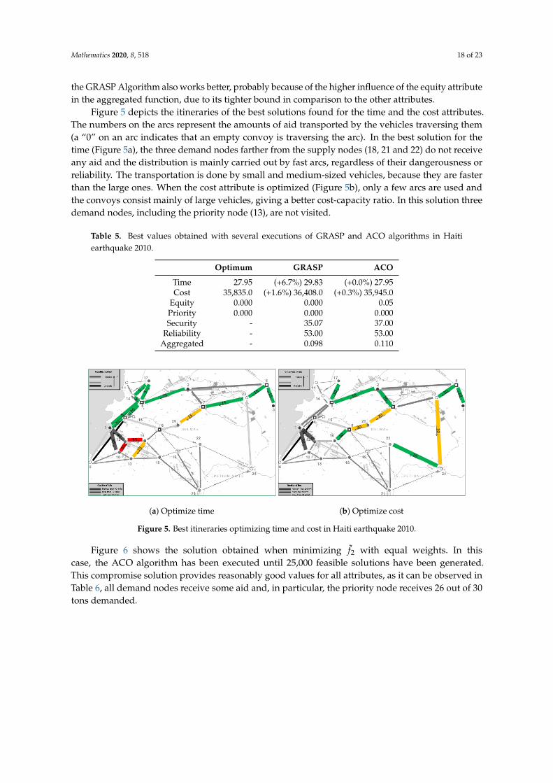
Table 5 shows the best values obtained among all tests performed during the experimentation—notonly the ten executions of the previous table—in the Haiti test case, together with the optimal values forthe attributes in which they are known. The optimal values for time and cost were obtained by usingthe static flow model described in [29], which although has some different assumptions, can serveas a reference for these two attributes that are measured in a very similar way. The ACO Algorithmprovides the assumed optimal value for the time attribute and stays very close to the optimum for thecost, substantially improving the results obtained with the GRASP Algorithm. For the priority and thereliability attributes, both algorithms provide the same values, and almost the same for the security,whereas for the equity attribute, the ACO Algorithm performs worse. For the aggregated function,

Mathematics 2020, 8, 518 18 of 23

the GRASP Algorithm also works better, probably because of the higher influence of the equity attributein the aggregated function, due to its tighter bound in comparison to the other attributes.

Figure 5 depicts the itineraries of the best solutions found for the time and the cost attributes.The numbers on the arcs represent the amounts of aid transported by the vehicles traversing them(a “0” on an arc indicates that an empty convoy is traversing the arc). In the best solution for thetime (Figure 5a), the three demand nodes farther from the supply nodes (18, 21 and 22) do not receiveany aid and the distribution is mainly carried out by fast arcs, regardless of their dangerousness orreliability. The transportation is done by small and medium-sized vehicles, because they are fasterthan the large ones. When the cost attribute is optimized (Figure 5b), only a few arcs are used andthe convoys consist mainly of large vehicles, giving a better cost-capacity ratio. In this solution threedemand nodes, including the priority node (13), are not visited.

Table 5. Best values obtained with several executions of GRASP and ACO algorithms in Haitiearthquake 2010.

Optimum GRASP ACO

Time 27.95 (+6.7%) 29.83 (+0.0%) 27.95Cost 35,835.0 (+1.6%) 36,408.0 (+0.3%) 35,945.0

Equity 0.000 0.000 0.05Priority 0.000 0.000 0.000Security - 35.07 37.00

Reliability - 53.00 53.00Aggregated - 0.098 0.110

55

(a) Optimize time (b) Optimize cost

Figure 5. Best itineraries optimizing time and cost in Haiti earthquake 2010.

Figure 6 shows the solution obtained when minimizing f̃2 with equal weights. In thiscase, the ACO algorithm has been executed until 25,000 feasible solutions have been generated.This compromise solution provides reasonably good values for all attributes, as it can be observed inTable 6, all demand nodes receive some aid and, in particular, the priority node receives 26 out of 30tons demanded.

Mathematics 2020, 8, 518 19 of 23

Figure 6. Best itineraries optimizing f̃2 in Haiti earthquake 2010.

Table 6. Best objective values optimizing f̃2 in Haiti earthquake 2010.

Time Cost Equity Priority Security Reliability

41.41 49,767.00 0.30 0.13 87.59 88.45

Finally, we summarize the results obtained in the Niger test case. As in the Haiti test case, GRASPand ACO have been executed ten times minimizing each objective independently and ten timesminimizing the aggregated function, running 1500 s per execution. Again, Table 7 shows the objectivevalues of the best and the worst solutions among the ten executions for each attribute, together withthe average and the standard deviation of the objective values of the ten solutions. The operationtime is given in hours, the cost in euros, and the security and the reliability in expected lost tons.Both algorithms provide optimal solutions for the equity and priority objectives in the ten executions.The ACO Algorithm performs slightly better than GRASP for the security and significantly better forthe remaining attributes—time, cost and reliability—and also for the aggregated function. The bestvalue obtained with ACO for the cost is only 1.6% higher than the assumed optimal value of the costattribute, which is EUR 63,240.0, obtained using the static flow model [28]. ACO is significantly betterfor the cost, the time, the reliability and the aggregated function. Despite the higher speed of GRASPgenerating feasible solutions in this test case—9000 on average per execution with GRASP versus 6400with ACO—ACO performance is much better than that of GRASP.

Table 7. Results obtained with ten executions per objective of GRASP and ACO algorithms in NigerFamine 2005.

GRASP ACO

Best Average Worst Std. dev. Best Average Worst Std. dev.Time 40.96 45.72 46.25 1.59 22.21 34.59 47.00 10.32Cost 64,860.0 65,196.9 65,497.5 238.3 64,250.0 64,389.2 64,852.5 164.7

Equity 0.000 0.000 0.000 0.000 0.000 0.000 0.000 0.000Priority 0.367 0.367 0.367 0.000 0.367 0.367 0.367 0.000Security 200.00 200.18 201.75 0.53 200.00 200.00 200.00 0.00

Reliability 789.10 809.96 830.30 11.87 763.10 764.54 765.60 0.60Aggregated 0.167 0.172 0.175 0.002 0.154 0.159 0.172 0.007

Mathematics 2020, 8, 518 20 of 23

It is remarkable that the number of feasible solutions generated using the same computation timeis lower in the Niger test case than in the Haiti test case, even though the logistic network is muchsmaller in the former. This is because there are other factors that influence the computation time as,for example, the structure of the network, the number and the location of the vehicles, the relationbetween the amount to be distributed and the total capacity of the vehicles, etc.

The proposed compromise solution for the Niger test case is shown in Table 8. All attribute valuesremain reasonably close to the best values obtained by optimizing each objective individually, exceptthe value for the priority objective. This is partially due to the high confrontation between the equityand priority attributes. For optimizing the priority attribute, the node with the highest priority level(Zinder) should receive all the demanded aid, which would lead to an inequitable distribution.

Table 8. Best objective values optimizing f̃2 in Niger famine 2005.

Time Cost Equity Priority Security Reliability

65.00 6,802,000.0 0.066 0.711 259.85 956.20

In summary, the results obtained in both test cases show that the ACO Algorithm is able toobtain good solutions for all attributes when optimizing each of them individually, together with goodcompromise solutions as well. In particular, it provides the best known solutions for several attributes,such as the operation time in the Haiti test case or the reliability of the itineraries in the Niger test case.In addition, the computational effort required by the ACO algorithm is quite reasonable, making itsuitable to solve realistic cases.

5.4. Managerial Insights

1. The security issues related to the distribution of humanitarian aid, mainly focused on avoidingpossible assaults to the vehicles performing the distribution operations in dangerous areas, are akey element in certain contexts, as for example war zones or extremely poor places. In thesesituations, it is frequently required that the vehicles involved are grouped forming convoys,as a protection mechanism and to allow escort details monitoring. This condition introducessignificant additional difficulties into the last mile distribution models that must be properlyaddressed, but it makes the models more realistic and useful. The proposed metaheuristicalgorithm can be used to obtain the precise distribution plan in an efficient way.

2. In this work, two case studies, regarding an earthquake and a famine, a rapid and a slow onsetdisaster, respectively, have been considered. However, the proposed model and solution methodcan be applied to any kind of disaster, especially to the ones occurring in unsecure environments.

6. Concluding Remarks

This paper addresses a humanitarian last mile distribution problem in response to a disaster.The distribution must be done under unsecure conditions, so the vehicles must travel in convoysto try to prevent assaults. Furthermore, there is uncertainty about the state of the roads, that mayhave been damaged by the disaster. The proposed model is multimodal, multidepot, allows splitdeliveries and multiple trips and provides the individual itineraries of the vehicles. Besides, the modelconsiders six performance criteria—time, cost, equity, priority, security and reliability—and is solvedby a compromise programming approach.

The main contribution of this paper is the proposed methodology to solve the model. We developan algorithm based on Ant Colony Optimization that considers several types of ants and pheromones.The methodology introduces the concept of effective pheromones to balance the elements of theprovided solutions and to diversify the set of obtainable solutions. This methodology is especiallyappropriate to approach routing problems in which the vehicles are required to travel in convoys,

Mathematics 2020, 8, 518 21 of 23

but some of its most novel elements, as it is the case of the effective pheromones, could also besuccessfully applied to many other complex distribution and routing problems.

The algorithm is tested on two realistic case studies of public domain, and its performanceis compared to that of the GRASP Algorithm, the only existing solution method in the literature.The ACO Algorithm performs well for all the objective functions tested in our experiments andprovides, for both test cases considered, the best solutions obtained to date for several attributes.In comparison with the available solution method in the literature—the GRASP Algorithm—in theHaiti test case, both algorithms have their own strengths, but in the Niger test case, ACO clearlyoutperforms GRASP. The computation time required to obtain good solutions is reasonable in all cases,proving that the ACO Algorithm can be perfectly applied in an emergency context. Furthermore,GRASP and ACO algorithms actually complement each other and could even be used in combinationin order to improve the quality of the final solutions provided to the decision makers.

One interesting future research line to continue this work comprises the development of astochastic model in which the possibility of suffering assaults or finding blocked roads could berepresented by random variables. Additionally, the design of simulation models to replicate realsituations and test different solution strategies could also be worth considering.

Author Contributions: Conceptualization, J.M.F., M.T.O. and G.T.; Methodology, J.M.F., M.T.O. and G.T.; Software,J.M.F.; Validation, J.M.F., M.T.O. and G.T.; Formal analysis, J.M.F., M.T.O. and G.T.; Investigation, J.M.F., M.T.O.and G.T.; Data curation, J.M.F., M.T.O. and G.T.; Writing—original draft preparation, J.M.F.; Writing—reviewand editing, M.T.O. and G.T.; Visualization, J.M.F., M.T.O. and G.T.; Project administration, M.T.O. and G.T. Allauthors have read and agreed to the published version of the manuscript.

Funding: This research was funded by the European Commission grant H2020 MSCA-RISE 691161 (GEO-SAFE),the Government of Spain grant MTM2015-65803-R and the Government of Madrid, grant S2013/ICE-2845.The APC was funded by the European Commission grant H2020 MSCA-RISE 691161 (GEO-SAFE).

Conflicts of Interest: The authors declare no conflict of interest.

References

1. Altay, N.; Green, W.G. OR/MS research in disaster operations management. Eur. J. Oper. Res. 2006,175, 475–493. [CrossRef]

2. Özdamar, L.; Ertem, M.A. Models, solutions and enabling technologies in humanitarian logistics. Eur. J.Oper. Res. 2015, 244, 55–65. [CrossRef]

3. Tomasini, R.; van Wassenhove, L. Humanitarian Logistics; Palgrave Macmillan: London, UK, 2009.4. Vitoriano, B.; Montero, J.; Ruan, D. Decision Aid Models for Disaster Management and Emergencies; Atlantis

Press: Paris, France, 2013.5. Pedraza-Martínez, A.J.; Van Wassenhove, L.N. Empirically grounded research in humanitarian operations

management: The way forward. J. Oper. Manag. 2016, 45, 1–10. [CrossRef]6. Besiou, M.; Pedraza-Martínez, A.J.; Van Wassenhove, L.N. OR applied to humanitarian operations. Eur. J.

Oper. Res. 2018, 269, 397–405. [CrossRef]7. Fiedrich, F.; Gehbauer, F.; Rickers, U. Optimized resource allocation for emergency response after earthquake

disasters. Saf. Sci. 2000, 35, 41–57. [CrossRef]8. Viswanath, K.; Peeta, S. Multicommodity maximal covering network design problem for planning critical

routes for earthquake response. Transp. Res. Rec. 2003, 1857, 1–10. [CrossRef]9. Kongsomsaksaku, S.; Yang, C.; Chen, A. Shelter location-allocation model for flood evacuation planning.

J. East. Asia Soc. Transp. Stud. 2005, 6, 4237–4252.10. Barzinpour, F.; Saffarian, M.; Makoui, A.; Teimoury, E. Metaheuristic Algorithm for Solving Biobjective

Possibility Planning Model of Location-Allocation in Disaster Relief Logistics. J. Appl. Math. 2014,2014, 239868. [CrossRef]

11. Yi, W.; Özdamar, L. A dynamic logistics coordination model for evacuation and support in disaster responseactivities. Eur. J. Oper. Res. 2007, 179, 1177–1193. [CrossRef]

12. Habib, M.S.; Sarkar, B. An Integrated Location-Allocation Model for Temporary Disaster Debris Managementunder an Uncertain Environment. Sustainability 2017, 9, 716. [CrossRef]

Mathematics 2020, 8, 518 22 of 23

13. Huang, M.; Smilowitz, K.; Balcik, B. Models for relief routing: equity, efficiency and efficacy. Transp. Res.Part E Logist. Transp. Rev. 2012, 48, 2–18. [CrossRef]

14. Holguín-Veras, J.; Pérez, N.; Jaller, M.; Van Wassenhove, L.; Aros-Vera, F. On the appropriate objectivefunction for post-disaster humanitarian logistics models. J. Oper. Manag. 2013, 31, 262–280. [CrossRef]

15. Gutjahr, W.J.; Nolz, P.C. Multicriteria optimization in humanitarian aid. Eur. J. Oper. Res. 2016, 252, 351–366.[CrossRef]

16. Ferrer, J.M.; Ortuño, M.T.; Tirado, G. A GRASP metaheuristic for humanitarian aid distribution. J. Heuristics2016, 22, 55–87. [CrossRef]

17. Balcik, B.; Beamon, B.M.; Smilowitz, K. Last mile distribution in humanitarian relief. J. Intell. Transp. Syst.2008, 12, 51–63. [CrossRef]

18. Nolz, P.C.; Semet, F.; Doerner, K.F. Risk approaches for delivering disaster relief supplies. OR Spectrum 2011,33, 543–569. [CrossRef]

19. Lin, Y.H.; Batta, R.; Rogerson, P.A.; Blatt, A.; Flanigan, M. A logistics model for emergency supply of criticalitems in the aftermath of a disaster. Socio-Econ. Plan. Sci. 2012, 45, 132–145. [CrossRef]

20. Bozorgi-Amiri, A.; Jabalameli, M.S.; Al-e Hashem, S.M.J.M. A multi-objective robust stochastic programmingmodel for disaster relief logistics under uncertainty. OR Spectrum 2013, 35, 905–933. [CrossRef]

21. Tirado, G.; Martín-Campo, F.J.; Vitoriano, B.; Ortuño, M.T. A lexicographical dynamic flow model for reliefoperations. Int. J. Comput. Int. Syst. 2014, 7, 45–57. [CrossRef]

22. Huang, K.; Jiang, Y.; Yuan, Y.; Zhao, L. Modeling multiple humanitarian objectives in emergency response tolarge-scale disasters. Transp. Res. Part E Logist. Transp. Rev. 2015, 75, 1–17. [CrossRef]

23. Ahmadi, M.; Seifi, A.; Tootooni, B. A humanitarian logistics model for disaster relief operation consideringnetwork failure and standard relief time: A case study on San Francisco district. Transp. Res. Part E Logist.Transp. Rev. 2015, 75, 145–163. [CrossRef]

24. Zhou, Y.; Liu, J.; Zhang, Y.; Gan, X. A multi-objective evolutionary algorithm for multi-period dynamicemergency resource scheduling problems. Transp. Res. Part E Logist. Transp. Rev. 2017, 99, 77–95. [CrossRef]

25. Maghfiroh, M.F.N.; Hanaoka, S. Last mile distribution in humanitarian logistics under stochastic anddynamic consideration. In Proceedings of the 2017 IEEE International Conference on Industrial Engineeringand Engineering Management (IEEM), Singapore, 10–13 December 2017; pp. 1411–1415.

26. Moreno, A.; Alem, D.; Ferreira, D.; Clark, A. An effective two-stage stochastic multi-triplocation-transportation model with social concerns in relief supply chains. Eur. J. Oper. Res. 2018,269, 1050–1071. [CrossRef]

27. Habib, M.S.; Sarkar, B.; Tayyab, M.; Saleem, M.W.; Hussain, A.; Ullah, M.; Omair, M.; Iqbal, M.W. Large-scaledisaster waste management under uncertain environment. J. Clean. Prod. 2019, 212, 200–222. [CrossRef]

28. Ortuño, M.T.; Tirado, G.; Vitoriano, B. A lexicographical goal programming based decision support systemfor logistics of Humanitarian Aid. TOP 2011, 19, 464–479. [CrossRef]

29. Vitoriano, B.; Ortuño, M.T.; Tirado, G.; Montero, J. A multi-criteria optimization model for humanitarian aiddistribution. J. Glob. Optim. 2011, 51, 189–208. [CrossRef]

30. Ferrer, J.M.; Martín-Campo, F.J.; Ortuño, M.T.; Pedraza-Martínez, A.J.; Tirado, G.; Vitoriano, B. Multi-criteriaoptimization for last mile distribution of disaster relief aid: Test cases and applications. Eur. J. Oper. Res.2018, 269, 501–515. [CrossRef]

31. Rizzoli, A.E.; Montemanni, R.; Lucibello, E.; Gambardella, L.M. Ant colony optimization for real-worldvehicle routing problems. Ann. Oper. Res. 2007, 1, 135–151. [CrossRef]

32. Yu, B.; Yang, Z.Z.; Xie, J.X. A parallel improved ant colony optimization for multi-depot vehicle routingproblem. J. Oper. Res. Soc. 2011, 62, 183–188. [CrossRef]

33. Zhang, L.Y.; Fei, T.; Zhang, X.; Li, Y.; Yi, J. Research about Immune Ant Colony Optimization in EmergencyLogistics Transportation Route Choice. In Communications and Information Processing; Zhao, M., Sha, J.,Eds.; Communications in Computer and Information Science; Springer: Berlin/Heidelberg, Germany, 2012;Volume 288, pp. 430–437.

34. Hong, J.; Diabat, A.; Panicker, V.V.; Rajagopalan, S. A two-stage supply chain problem with fixed costs:An ant colony optimization approach. Int. J. Prod. Econ. 2018, 204, 214–226. [CrossRef]

35. Yi, W.; Kumar, A. Ant colony optimization for disaster relief operations. Transp. Res. Part E Logist. Transp. Rev.2007, 43, 660–672. [CrossRef]

Mathematics 2020, 8, 518 23 of 23

36. Saeidian, B.; Mesgari, M.S.; Pradhan, B.; Ghodousi, M. Optimized Location-Allocation of Earthquake ReliefCenters Using PSO and ACO, Complemented by GIS, Clustering, and TOPSIS. ISPRS Int. J. Geo-Inf. 2018,7, 1–25. [CrossRef]

37. Cochrane, J.L.; Zeleny, M. Multiple Criteria Decision Making; University of South Carolina Press: Columbia,SC, USA, 1973.

38. Dorigo, M.; Maniezzo, V.; Colorni, A. Ant system: optimization by a colony of cooperating agents. IEEE Trans.Syst. Man Cybern. Part B Cybern. 1996, 26, 29–41. [CrossRef] [PubMed]

39. Dorigo, M.; Blum, C. Ant colony optimization theory: A survey. Theor. Comput. Sci. 2005, 344, 243–278.[CrossRef]

40. Zhao, N.; Wu, Z.; Zhao, Y.; Quan, T. Ant colony optimization algorithm with mutation mechanism and itsapplications. Expert Syst. Appl. 2010, 37, 4805–4810. [CrossRef]

41. Chandra Mohan, B.; Baskaran, R. A survey: Ant Colony Optimization based recent research andimplementation on several engineering domain. Expert Syst. Appl. 2012, 39, 4618–4627. [CrossRef]

42. Dorigo, M.; Gambardella, L.M. Ant colony system: a cooperative learning approach to the traveling salesmanproblem. IEEE Trans. Evol. Comput. 1997, 1, 53–66. [CrossRef]

43. Ford, L.R.; Fulkerson, D.R. Maximal flow through a network. Can. J. Math. 1956, 8, 399–404. [CrossRef]44. United Nations Office for the Coordination of Humanitarian Affairs (OCHA). Available online: https:

//www.unocha.org/ (accessed on 17 March 2020).45. World Food Programme (WFP) Emergency Preparedness and Response. Available online: https://www.

wfp.org/emergency-preparedness-and-response (accessed on 17 March 2020).46. Vitoriano, B.; Ortuño, M.T.; Tirado, G. HADS, a goal programming-based humanitarian aid distribution

system. J. Multi-Crit. Decis. Anal. 2009, 16, 55–64. [CrossRef]47. Fondo de Ayuda Humanitaria y de Emergencias de Farmamundi (FAHE). Memoria. 2005. Available online:

http://www.farmaceuticosmundi.org/farmamundi/descargas/pdf/memoria_2005_fahe.pdf (accessed on17 March 2020).

c© 2020 by the authors. Licensee MDPI, Basel, Switzerland. This article is an open accessarticle distributed under the terms and conditions of the Creative Commons Attribution(CC BY) license (http://creativecommons.org/licenses/by/4.0/).