a near-wall turbulence model and its application to fully ... · a near-wall turbulence model and...
TRANSCRIPT

NASA Technical Memorandum 101399 ICOMP-88-20
A Near-Wall Turbulence Model and Its Application to Fully Developed Turbulent Channel and Pipe Flows
( k A S A - T H - I C - 1 3 9 9 ) A YiAFt-UALL IUBBULEHCE N89-12741 G C D E L A N G ITS A Z C Z J C A ' i I C I I C f U I Y DEVBLCPED 'ICHBULEY'I CHAhbEL A l l D F l P E € I C L S I b A S A ) 5 1 p CSCL 20D Unclas
G3/3U 01772C8
s.-w. Kim fiastitute for Computational Mechanics in Propukrion Lewis Research Center Cleveland, Ohio
November 1988
https://ntrs.nasa.gov/search.jsp?R=19890004370 2018-06-14T22:44:57+00:00Z

A NEAR-WALL TURBULENCE MODEL AND ITS APPLICATION TO
FULLY DEVELOPED TURBULENT CHANNEL AND PIPE FLOWS
S.-W. Kim Institute for Computational Mechanics in Propulsion
Lewis Research Center Cleveland, Ohio 44135
Summary
A near-wall turbulence model and its incorporation into a multiple-
time-scale turbulence model are presented in this report.
the conservation of mass, momentum, and the turbulent kinetic energy
equations are integrated up t o the wall; and the energy transfer rate and
the dissipation rate inside the near-wall layer are obtained from algebraic
equations. The algebraic equations for the energy transfer rate and the
dissipation rate inside the near-wall layer have been obtained from a
k-equation turbulence model and the near wall analysis.
turbulent channel flow and fully developed turbulent pipe flows were solved
using a finite element method to test the predictive capability of the
turbulence model. The computational results compared favorably with
experimental data. It is also shown that the present turbulence model
could resolve the over-shoot phenomena of the turbulent kinetic energy and
the dissipation rate in the region very close to the wall.
In the method,
A fully developed
*Work funded under Space Act Agreement C99066G.

CP1
ct1
c/Jf
P C
f/J
f e
k
kp kt
k+
Pr
Rt
r
U
US
"7 - U' 2
- u'v'
u"+
V
VS
Y
Y+
e
'P
Nomenclature
Turbulence model constants for e equation, (1=1,3)
Turbulence model constants for et equation, (1==1,3)
A constant coefficient ( -0 .09)
P
A coefficient used in eddy viscosity equation
Wall damping function for eddy viscosity equation
Wall damping function for dissipation rate
Total turbulent kinetic energy , (k=%+kt)
Turbulent kinetic energy of eddies in the production range
Turbulent kinetic energy of eddies in the dissipation range
Normalized turbulent kinetic energy (-k/ur2)
Production rate of turbulent kinetic energy
Turbulent Reynolds number ( - k 2 / ( v e ) )
Radial distance
Time averaged velocity
Non-dimensional velocity (-u/u,>
Friction velocity ( = J ( , " / p ) )
Normal Reynolds stress, R.M.S. value of the fluctuating axial velocity
Reynolds stress
Normalized Reynolds stress (=u"/ur2)
Time averaged velocity in the y-coordinate direction
turbulence velocity scale
normal distance from the wall
Wall coordinate (=u,y/v)
Dissipation rate
Transfer rate of turbulent kinetic energy from the production range to the dissipation range
2

K.
I
I,
Y
”t
QP
akt
“ep
Q€t
TW
Dissipation rate of turbulent kinetic energy
Dissipation rate inside the near-wall layer
Non-dimensional dissipation rate (-vc/u, 4 )
von Karman constant
turbulence length scale
mixing length
kinematic viscosity of fluid
turbulent eddy viscosity
Turbulent Prandtl number for $ equation
Turbulent Prandtl number for kt equations
Turbulent Prandtl number for ep equation
Turbulent Prandtl number for et equation
Wall shearing stress
3

Introduction
For wall bounded turbulent flows in the equilibrium state, the
logarithmic velocity profile prevails in the near-wall region1. The most
widely used wall function methods in numerical calculations of turbulent
flows have been derived from the logarithmic velocity profile based on the
experimental observation that the turbulence in the near-wall region can be
described in terms of the wall shearing stress. The wall function methods
are not valid at or near the separation point since the turbulence in this
region can not be described in terms of the wall shearing stress. For
unsteady turbulent flows, the logarithmic velocity profile no longer
prevails in the near-wall or in the wake region 2 , therefore the wall
function methods can not be applied. Other occasions in which the wall
function methods become invalid include low turbulent Reynolds number flows
in which the effect of molecular viscosity become important and flows over
surfaces with mass injection and/or suction. The objective of this study is
to eatablishes a near-wall turbulence model which can be used in place of
wall function methods. Further application of the present near-wall
turbulence model for complex turbulent flows such as the turbulent flow
over a curved hill3 and the turbulent boundary layer - shock wave
interaction^^-^ can be found in Reference 6. Numerous efforts have been made to include the near-wall low turbulent
Reynolds number region in turbulent flow computations. Various turbulence
models which include the near-wall low turbulence region can be classified
as two- or multi-layer turbulence rnodels7-l0, low Reynolds number
turbulence models, and partially low Reynolds number turbulence models. The
advantages and disadvantages of these various methods are discussed in the
following.
4
In the two- or multi-layer turbulence models, the turbulence in the
near-wall layer has been described by algebraic e~pressions~-~~. In these
turbulence models, the turbulent kinetic energy and the dissipation rate in
the near-wall layer have been constructed by piecewise continuous
functions. As a consequence, the computational results may depend on the
location of the partition between the near-wall layer and the fully
turbulent region8. In some of these methods, a quadratic variation of the
turbulent kinetic energy has been assumed in the near-wall region and the
dissipation rate has been derived from the logarithmic velocity profile
equation 4 . This class of methods is advantageous in studying the near-wall
turbulence structure for equilibrium turbulent flows. However, these
methods become invalid if the logarithmic velocity profile does not prevail
in the near wall region. The underlying assumption that the turbulent
kinetic energy is proportional to square of the distance from the wall
inside the near-wall layer is also questionable, since the quadratic
variation of the turbulent kinetic energy is valid only inside the viscous
sublayer and become invalid as the fully turbulent region is approached.
In the low Reynolds number turbulence models, the high Reynolds number
turbulence models have been extended to include the near-wall low
turbulence effectll. In this class of methods, the near-wall low turbulence
effects have been incorporated into the high Reynolds number turbulence
models by using the wall damping functions. These wall damping functions
have been derived mostly from numerical experiments in such a way that the
low Reynolds number turbulence models could reproduce the experimentally
observed turbulent flow phenomena in the near-wall region. In this class of
methods, a significant number of grid points has to be assigned in the near
wall region in order to resolve the stiff dissipation rate equation.
5
Aside from the above two classes of methods, a new approach has been
used in Chen and Patel12 to solve complex turbulent flow. In the method,
only the turbulent kinetic energy equation of the k-E turbulence model has
been extended to include the near-wall low turbulence effect and the
dissipation rate inside the near-wall layer has been prescribed
algebraically.
k-equation turbulence model13. Thus the turbulent kinetic energy and the
dissipation rate varies smoothly from the wall toward the outside fully
turbulent region. In this case, it would be more appropriate to classify
the turbulence model as a partially low Reynolds number turbulence model to
distinguish it from the other two classes of methods.
The dissipation rate equation has been obtained from a
It has been shown previously that the high Reynolds number
multiple- time-scale turbulence model16 yielded significantly improved
computational results for a class of complex turbulent flows such as a wall
jet flow17, a wake-boundary layer interaction flow18, a confined coaxial
jet without swirl19, and a confined coaxial swirling jet20, to name a few.
In the single-time-scale turbulence models such as the k-e turbulence
models and the Reynolds stress turbulence models, a single-time-scale is
used to express both the turbulent transport and the dissipation of the
turbulent kinetic energy. However, this practice is inconsistent with
physically observed turbulence in a sense that the turbulent transport is
related to the time scale of energy containing large eddies and the
dissipation rate of turbulent kinetic energy is related to the time scale
of fine scale eddies in the dissipation range. The single time-scale
turbulence models have been used most widely and yielded quite accurate
computational results for many turbulent flows; however, the predictive
capability degenerated significantly for complex turbulent flows with
6

strong inequilibrium turbulence. In the multiple-time-scale turbulence
models16 9 21-24, the turbulent transport of mass and momentum has been
described using the time scale of the large eddies; and the dissipation
rate has been described using the time scale of the fine scale eddies. The
improved computational results obtained by using the multiple-time-scale
turbulence model for complex turbulent flows can be attributed to the above
discussed physically consistent nature of the turbulence models.
It has been shown that the k-equation turbulence models yielded highly
accurate computational results for a class of standard turbulent boundary
layer flows25, turbulent flows with drag reduction26, an unsteady fully
developed turbulent channel flow27, and fully developed unsteady turbulent
pipe flows2. However, the k-equation turbulence model itself is less useful
for separated and/or swirling turbulent flows with complex geometry due to
lack of a systematic method to evaluate the turbulence length scale.
The near-wall turbulence model presented in this report belongs to the
partially low Reynolds number turbulence models. In the model, the
turbulence structure in the near-wall low turbulence region has been solved
by extending the turbulent kinetic energy equations to include the low
turbulence effect and the energy transfer rate and the dissipation rate
have been prescribed algebraically. The energy transfer rate and the
dissipation rate equations in the near-wall layer have been obtained from
the k-equation turbulence model13. The rest of the flow domain has been
solved by the high Reynolds number multiple-time-scale turbulence model 16 .
Further advantages of this approach originating from physical and numerical
considerations are discussed in the following section.
Example problems considered include: a fully developed turbulent
channel flow14 at Reynolds number (Re) of 30,800 and turbulent pipe flows15
7

for Re - 50,000 and 500,000. The computational results compared favorably with experimental data globally. More importantly, significantly improved
computational results for the turbulence structure in the near-wall region,
including the experimentally observed over-shoot phenomena of the turbulent
kinetic energy and the dissipation rate, have been obtained.
NEAR-WALL TURBULENCE MODEL
The turbulence in external flows and that in near-wall boundary layer
flows have quite different length scales28 9 29. The turbulence length scale
of the external flows is related to the flow field characteristics. On the
other hand, the turbulence length scale of boundary layer flows is strongly
related to the normal distance from the wall. This nature of the wall
bounded turbulent flows can be described quite naturally by the partially
low Reynolds number turbulence models. The same purpose could be achieved
by the low Reynolds number turbulence models as more experimental data
become available. However, the gradient of the dissipation rate is the most
stiff in the near-wall region, and a great number of grid points has to be
used in the region for the low Reynolds number turbulence models to resolve
the dissipation rate. Therefore, the partially low Reynolds number
turbulence models seem to be more advantageous as compared with the low
Reynolds number turbulence models, unless the low Reynolds number
turbulence models can describe the wall bounded turbulent flows more
accurately.
Eddy Viscosity Equation in the Near-Wall Region -
In the Prandtl-Kolmogorov theory, the eddy viscosity is given as;
Vt = vsR
8

where vs and R are the turbulence velocity and length scales, respectively
The velocity scale has been most frequently represented by the square root
of the turbulent kinetic energy. The turbulent length scale in the fully
turbulent region of wall bounded turbulent flows is given
where cpf (lO.09) is a constant, Rm is the mixing length, IC is the von
Karman constant, and y is the normal distance from the wall. The fully
turbulent region extends from y+=30 up to y+=-300, where y+=u'y/u is the
wall coordinate, U~==J(T~/~) is the friction velocity, rW is the wall
shearing stress, and v is the kinematic viscosity of fluid. Thus the
turbulent eddy viscosity in this fully turbulent region is given as;
ut - k1I2R ( 4 )
where k is the turbulent kinetic energy.
The instantaneous velocity in the viscous sublayer region can be
written asll;
I ut = aly + a2y2 + . . . . v' = b2y2 + . . . . w' = c1y + c2y2 + . . . .
(5)
where the coefficients ai, bi, and ci are functions of time such that ai =
9

bi - ci = 0, and the over-bar denotes time average. Note that the
fluctuating normal velocity component grows in proportion to the square of
the distance from the wall due to the wall proximity effect. The turbulence
in the very closed to the wall region, i.e., y=O can be written as;
1 1 I - - - I - - k = - (uI2 + vt2 + wI2) = - (a12 + el2) y2 + . . . .
2 2
- u’v’ = alb2y - 3
- where E is the dissipation rate, and u’v’ is a component of the Reynolds
stress. Due to the difficulty in measuring the turbulence quantity in the
very close to the wall region, there exist only a limited number of
experimental data to support the above analysis. For example, the
experimental data compiled by Cole30 showed that the turbulent kinetic
energy grows in proportion to the square of the distance from the wall.
In the Boussinesq eddy viscosity assumption, the Reynolds stress is
given as;
aui auj
axj axi - Ui‘Uj‘ = ut (- + -) ( 9 )
Very close to the wall, the velocity gradient is a constant. Thus eqs. ( 8 )
and (9) indicate that the eddy viscosity is in proportion to the third
power of the distance from the wall; whereas, eqs. (2-4) and ( 6 ) indicate
10

t ha t the eddy viscosi ty is proportional t o the square of the distance from
the w a l l i n the viscous sublayer region. This difference is a t t r ibu ted t o
the f a c t t ha t the molecular viscosi ty dominates i n the viscous sublayer
region and t h a t the eddy viscosi ty dominates i n the f u l l y turbulent region.
The turbulent v i scos i ty equation can be modified t o include the e f f ec t of
molecular v i scos i ty i n the viscous sublayer region as ;
Thus the damping function f, has t o be a l inear function of the distance
from the wall and has t o approach unity as the f u l l y turbulent region is
approached.
Note t h a t the eddy viscosi ty i n the Prandtl mixing length theory is
proportional t o the fourth power of the distance from the wall , i . e . ;
where &,-ny(l-exp(y+/A+)) and A+ is the w a l l damping fac tor . There also
ex i s t s a few low Reynolds number turbulence models i n which the eddy
v iscos i ty var ies i n proportion t o the fourth power of the distance from t h e
wal l , see Reference 11 for more discussion.
In the f u l l y turbulent region of wall bounded turbulent flows, the
d iss ipa t ion rate is re la ted t o the mixing length o r the turbulence length
scale a s ;
11

- Cpf - a
The dissipation rate given as eq. (12) vanishes in the region very
close to the wall. However, the experimentally observed dissipation rate
approaches a constant value in the region, see eq. .(7). Two slightly
different approaches have been used to approximate the dissipation rate in
the near-wall region. In the k-equation turbulence model of Gibson et.
al. 25, Hassid and Poreh26, and Acharya and Reynolds27, the dissipation rate
in the near-wall layer has been obtained by linear combination of eqs. (7)
and (12), and is given as;
k312 2uk EW E C , , f 3 1 4 f,h - + -
KY Y2
where f,h is a wall damping function varying from null on the wali to unit
in the fully turbulent region. On the other hand, in the k-equation
turbulence model of Wolfshtein13, the dissipation rate in the near-wall
layer was given as;
1 c,,f314k312 €w = -
f € KY
where f, has been chosen so that the dissipation rate would approach to the
value given in eq. (7) for y=O and f, take unit value in the fully
turbulent region. The fully turbulent region with equilibrium turbulence
extends from y+=30 to y+=300 for wall bounded flows. Eq. (14) has also been
used in the partially low Reynolds number k-c turbulence model of Chen and
12

Patel’* for numerical computations of separated turbulent flows. Eq. (14 )
has been used in the present study, and partial justification is presented
in the following paragraph.
Consider the turbulent kinetic energy equation given as;
where Uk is the turbulent Prandtl number for the k-equation and
Pr--u.’u ‘(aui/axj) is the production rate. Very close to the wall (y=O),
the molecular viscosity dominates over the turbulent eddy viscosity, and the
convection term is found to be negligible compared with the diffusion term
from an order of magnitude analysis1. Then the analytical solution of eq.
(15) for y=O is given as eq. (7 ) . For y>O, the turbulent eddy viscosity
% j
grows in proportion to the third power of the distance from the wall. Hence
it can be argued that the dissipation rate given as eq. (7 ) , which is the
analytical solution of eq. (15) for y=O, may valid only at very close to
the wall. However, the dissipation rate given as eq. (7) retains
significant magnitude even in the fully turbulent region, i.e. y+=lOO. For
this reason, the work of Wolfshtein13 and Chen and Patel12 has been
followed herein. In the present study, the near-wall damping function f o r
eq. (14) is given as;
where Rt-k2/(ve) is the turbulent Reynolds number and Ae=c,f3/2/(2n2). For
y=O, eq. (14) takes the limit value given as eq. (7).
13

Substituting eq. (12) into eq. (10) yields:
k2 Vt - Cpf f, -
E
and substituting ew, eq. (14), for e in eq. (17) yields the eddy viscosity
equation for the near-wall layer given as;
k2
‘ W Vt = Cpf f, -
where f,=l-exp(A1+/Rt + A2Rt2) is a linear function of the distance from the
wall in the viscous sublayer region and become unity in the fully turbulent
region. AI-0.025 and A2-0.00001 have been used for the near wall layer i n
the present study.
For near-wall equilibrium turbulent flows, the production rate is
approximately equal to dissipation rate (et), and hence the energy transfer
rate ( e ) from the low wave number production range to the high wave number
dissipation range has to be approximately equal to both of them. The energy
transfer rate and the dissipation rate inside the near-wall layer are given
P
as;
1 c,f3I4 k3I2
“Y €P - ‘t - ‘w - -
f e
Note that the production rate vanishes on the wall and grows to full
strength at y+-15. Hence eq. (19) may not be a good approximation for
O<y+<15. However, use of the vanishing boundary condition for the
14

turbulent kinetic energy on the wall yields the growth rate of the
turbulent kinetic energy and the production rate which is in good agreement
with experimental data as well as theoretical analysis.
Multiple-Time-Scale Turbulence Eauations
For clarity, the partially low Reynolds number multiple-time-scale
turbulence equations are summarized below. The partition between the
near-wall region and the fully turbulent outer region can be located
between y+
kinetic energy equations for the entire flow domain are given as;
greater than 40 and less than 300 approximately. The turbulent
akt a ut akt ( ( v + -) - ) = €p - €t 9- - -
axj axj Okt axj
where uj is the time averaged velocity in the j-th spatial coordinate
direction, Y is the kinematic viscosity of the fluid, vt is the turbulent
eddy viscosity, and Ukp=0.75 and Ukt-0.75 are the turbulent Prandtl numbers
for the 5 and kt equations, respectively. The energy transfer rate and the dissipation rate in the near-wall
layer are given as eq. (19). The convection-diffusion equations for the
energy transfer rate and the dissipation rate in the rest of the flow
domain are given as;
15

P where u
and Et equations, respectively, and c (1=1,3) and ctJ (1=1,3) are
turbulence model constants. These model constants are given as; cpl-0.21,
cp2-1.24, cP3= 1.84, ct1=0.29, ct2= 1.28, and ct3-1.66. Detailed derivation
of these model constants can be found in Reference 1 6 .
-1.15 and ~ ~ ~ - 1 . 1 5 are the turbulent Prandtl numbers for the E EP
PI
The eddy viscosity equation in the near-wall region is given as eq.
(13); and the eddy viscosity in the rest of the flow domain is given as;
k2 "t - Cpf-
'P
COMPUTATIONAL RESULTS
The turbulent boundary layer flows were solved by a finite element
method3'. It has been shown in Reference 31 that the finite element method
could solve a wide range of laminar boundary layer flows, such as the
Blasius flat plate flow, the retarded Howarth flow, flow over a wedge,
plane stagnation flow, flow over a circular cylinder, flow in the wake of a
flat plate, uniform suction flow over a flat plate, flow over a cone, and
flow over a sphere, as accurately as any available numerical methods
including the semi-analytical methods (i.e., a fourth-order Runge-Kutta
method1). Convergence study of the finite element method can be found in
reference 31, and implementaion of the method for turbulent flows can be
16

found in Reference 32. For completeness, the computational procedure
relevant to the present study is described briefly below.
In each iteration, the momentum equation and the turbulence equations
were solved sequentially with under-relaxation. The systems of equations
have been solved iteratively until the maximum relative error of each
turbulent flow variable became less than the specified convergence
criterion for each flow variable. Each system of equations was solved by a
penta-diagonal matrix algorithm (PDMA). Since the discrete system of
equations contained five diagonal entries, the PDMA yielded exact solution
for each system of equations. The convergence criterion used is given as;
where i (=u, kp, eP, kt, or et) denotes each flow variable; Ai denotes the
maximum magnitude of the i-th flow variable; N denotes the number of
degrees of freedom for each flow variable; e=l~lO-~ has been used for
velocity; and e-5~10'~ has been used for the rest of flow variables.
1. Fullv DeveloDed Channel Flow
The experimental data for the fully developed channel flow can be
found in Laufer14. The Reynolds number based on the center line mean
velocity (7 .07 m/sec) and the half of the channel width (0.0635 meters) was
approximately 30,800. The partition between the near-wall layer and the
fully turbulent region has been located at y+=lOO.'The near-wall layer has
been discretized by 20 grid points; and the rest of the flow domain, by 40
grid points. The Dirichlet boundary condition (u - prescribed at the wall; and the vanishing gradient
kp = kt = 0) has been
boundary condition, at
1 7

the center line of the channel. The pressure gradient estimated from the
pressure measurement and the wall shearing stress measurement were -1.41
kg-m/sec2-m3 and -1.40 kg-m/sec2-m3, respectively. In the present
computation, dp/dx = -1.405 kg-m/sec2-m3 has been used. The converged
solution has been obtained after approximately 400 iterations.
The computational results for the velocity, the turbulent kinetic
energy, and the Reynolds stress are compared with the experimental data in
Figure 1. The velocity profile compared less favorably with the
experimental data. The under-predicted velocity profile may due to the
inaccurate pressure gradient. The magnitude and location of the maximum
turbulent kinetic energy compared favorably with experimental data. It can
be seen from the Reynolds stress profile that the present turbulence model
yielded correct distribution of the turbulent viscosity.
The normalized velocity, the turbulent kinetic energy, and the
Reynolds stress inside the near-wall layer are shown in Figure 2; and the
normalized dissipation rate, the ratio of Pr/ct, and the wall damping
function are shown in Figure 3 . The calculated magnitude and the location
of the overshoots of the turbulent kinetic energy and the dissipation rate
were in good agreement with the experimental data. The rest of
computational results such as the ratio of production rate to dissipation
rate of the turbulent kinetic energy and the wall damping function compared
favorably with the semi-emperical data.ll It is shown in Reference 11 that
only a few low Reynolds number turbulence models could yield the turbulent
kinetic energy profile with overshoot in the near-wall region. It can be
found in Reference 32 that the global computational results obtained by
using various turbulence models with wall function methods compared
satisfactorily with experimental data. However, the correct magnitude of
18
the overshoot of the turbulent kinetic energy and the dissipation rate have
seldom been obtained.
2 . Fully DeveloDed Pipe Flows
The fully developed pipe flows at Reynolds numbers of 50,000 and
500,000 are considered below. The experimental data can be found in
Laufer14. The Reynolds number was based on the diameter of pipe (0.24688
meters) and the center line mean velocity. The center line velocities were
3.048 m/sec and 30.48 m/sec for Re=50,000 and 500,000, respectively. In
each case, the partition between the near-wall layer and the fully
turbulent region has been located at y+=lOO. For Re=50,000, the near -wall
layer has been discretized by 20 grid points; and the rest of the flow
domain, by 40 grid points. For Re-500,000, the near-wall layer has been
discretized by 20 grid points; and the rest of the flow domain, by 60 grid
points. For both cases, the Dirichlet boundary condition (u - kp - k, - 0 )
has been prescribed at the wall; and the vanishing gradient boundary
condition, at the center line of the pipe. The pressure gradients estimated
from the pressure measurements were -0.32 kg-m/sec2-m3 and -23.05
kg-m/sec2 -m3 for Re-50,000 and 500,000, respectively. The converged
solutions have been obtained after approximately 450 iterations for both
cases.
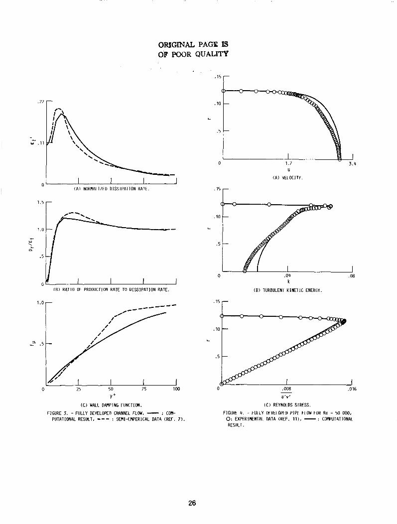
The computational results for the velocity, the turbulent kinetic
energy, and the Reynolds stress for Re-50,000 are compared with
experimental data in Figure 4 . For this case, the computational results
compared favorably with the experimental data. The Reynolds stress profile
was slightly under-predicted, however, the difference was negligible. The
normalized velocity, the turbulent kinetic energy, and the Reynolds stress
19

inside the near-wall layer are shown in Figure 5 ; and the normalized
dissipation rate, the ratio of Pr/et, and the wall damping function are
shown in Figure 6 . The calculated magnitude and the location of the
overshoots of the turbulent kinetic energy and the dissipation rate were in
excellent agreement with the experimental data.
The computational results for the velocity, the turbulent kinetic
energy, and the Reynolds stress for Re-500,000 are compared with
experimental data in Figure 7 . It was found that the mean velocity profile
was severely under-predicted. Again, this may due to the inaccurate
pressure gradient as in the fully developed channel flow case. The
thickness of the near-wall layer (i.e., y+<lOO) for Re-500,000 case was
approximately one order of magnitude smaller than that of Re-50,000 case.
Both the calculated and the measured turbulent kinetic energy profiles
exhibited strong peak in the region very close to the wall.
The normalized velocity, turbulent kinetic energy, and Reynolds stress
inside the near-wall layer are shown in Figure 8 ; and the normalized
dissipation rate, ratio of Pr/ct, and wall damping function are shown in
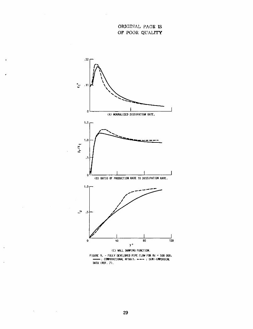
Figure 10. Again, the calculated magnitude and the location of the
overshoots of the turbulent kinetic energy and the dissipation rate were in
excellent agreement with the experimental data.
Conclusions and Discussion
A near-wall turbulence model and numerical computations of fully
developed turbulent channel flows and pipe flows using a partially low
Reynolds number multiple-time-scale turbulence model have been presented.
It has been shown that the present turbulence model yielded accurate
computational results for the example flows considered. The correct
20

magnitude and location of the overshoots of the turbulent kinetic energy
and the dissipation rate have been obtained only by a few low Reynolds
number turbulence models1'; and have seldom been obtained by the two- or
multi-layer turbulence models33. The turbulent kinetic energy and the
dissipation rate overshoots obtained by using the present turbulence model
were in excellent agreement with experimental data. The rest of the
computational results in the near-wall region such as the normalized
velocity profile, the Reynolds stress profile, the ratio of Production rate
to dissipation rate, and the wall damping function compared favorably with
experimental data.
In the two- or multi-layer turbulence models, the turbulent kinetic
energy in the near-wall layer is constructed by piecewise continuous
functions; and the dissipation rate, by discontinuous functions. In the
partially low Reynolds number turbulence models and in the low Reynolds
number turbulence models, the turbulent kinetic energy and the dissipation
rate vary smoothly from the wall toward the outside fully turbulent region.
In this regard, the partially low Reynolds number turbulence models and the
low Reynolds number turbulence models are more consistent with the
experimentally observed distribution of the turbulent kinetic energy and
the dissipation rate than the two- or multi-layer turbulence models are. A
significant number of grid points has to be assigned in the near-wall layer
for numerical computation of turbulent flows with the low Reynolds number
turbulence models. However, with the use of partially low Reynolds number
turbulence models, less number of grid points need to be assigned inside
the near-wall layer and the stiff dissipation rate in the region need not
be solved numerically. Therefore, many
robust and more efficient with the use
numerical codes can be made more
of the partially low Reynolds number
21

turbulence models.
References
1.
2.
3.
4.
5.
6 .
7.
8.
9.
10
White, F. M., Viscous Fluid Flow, McGraw-Hill, New York, 1974.
Tu, S . W., and Ramaprian, B. R., "Fully Developed Periodic Turbulent Pipe Flow. Part I, Main Experimental Results and Comparison with Predictions," J. Fluid Mechanics, Vol. 137, pp. 31-58, 1983.
Baskaran, V., Smits, A. J., and Joubert, P. N., "A Turbulent Flow over a Curved Hill, Part I. Growth of an Internal Boundary Layer," J. Fluid Mech., Vol. 182, pp. 47-83, 1987.
Bachalo, W. D., and Johnson, D. A., "An Investigation of Transonic Turbulent Boundary Layer Separation Generated on an Axisymmetric Flow Model," AIAA Paper 79-1479, 1979.
Horstman, C. C., Settles, G. S . , Bogdonoff, S . M., and Hung, C. M., "Reynolds Number Effects on Shock-Wave Turbulent Boundary-Layer Interactions," J. AIM, Vol. 15, No. 8, pp. 1152-1158, 1977.
Kim, S.-W., "Application of a Near-Wall Turbulence Model to Shock Wave - Turbulent Boundary Layer Interaction Flows," In preparation, 1988.
Amano, R. S . , "Development of a Turbulent Near-Wall Model and Its Application to Separated and Reattached Flows," Numerical Heat Transfer, Vol. 7, pp. 59-75, 1984.
Gorski, J. J., "A New Near-Wall Formulation for the k-r Equations of Turbulence," AIAA-86-0556, AIM 24th Aerospace Sciences Meeting, Reno, Nevada, 1986.
Kim, S.-W., and Chen, C.-P., "A Finite Element Computation of Complex Turbulent Boundary Layer Flows with a Two-Layer Multiple-Time-Scale Turbulence Model," NASA CR, In print, 1988.
Viegas, J. R., Rubesin, M. W., and Horstman, C. C., "On the Use of Wall Functions as Boundary Conditions for Two-Dimensional Separated Compressible Flows," AIAA-85-0180, AIAA 23rd Aerospace Sciences Meeting, Reno, Nevada, 1985.
11. Patel, V. C., Rodi, W., and Scheuerer, G., "Turbulence Models for Near Wall and Low Reynolds Number Flows: A Review", J. AIM, 23, pp. 1308-1319 (1985).
12. Chen, H. C., Patel, V. C., "Practical Near-Wall Turbulence Models f o r Complex Flows Including Separation," AIAA-87-1300, 1987.
13. Wolfshtein, M., "The Velocity and Temperature Distribution in One-Dimensional Flow with Turbulence Augmentation and Pressure
22

Gradient," Int. J. Heat and Mass Transfer, Vol 12, pp. 301-318, 1969.
14. Laufer, J., "Investigation of Turbulent Flow in a Two-Dimensional Channel", NACA CR-1053, 1949.
15. Laufer, J., "The Structure of Turbulence in Fully Developed Pipe Flow", NACA TR-1174, 1954.
16. Kim, S.-W., and Chen, C.-P., "A Multiple-Time-Scale Turbulence model Based on Variable Partitioning of the Turbulent Kinetic Energy Spectrum", NASA CR-179222, In print, 1987, See also AIM-88-0221, AIAA Aerospace Sciences Meeting, Reno, Nevada, 1988.
17. Irwin, H. P. A. H., "Measurements in a Self-preserving Plane Wall Jet in a Positive Pressure Gradient", J. Fluid Mech., Vol. 61, pp. 33-63, 1973.
18. Tsiolakis, E. P., Krause, E., and Muller, U. R., "Turbulent Boundary Layer-Wake Interaction" in Bradbury, L. J. S., Durst, F., Launder, B. E., Schmidt, F. W., and Whitelaw, J. H., Eds., Turbulent Shear Flows, Vol. 4, Springer-Verlag, New York, 1983.
19. Kim, S.-W., and Chen, C.-P., "A Review on Various Flow-Solid Interaction Analysis Methods with Emphasis on Recent Advances in Turbulence Models and Flow Analysis Methods," AIAA-88-3685, First National Fluid Dynamics Conference, Cincinnati, Ohio, 1988.
20. Roback, R. and Johnson B. V., "Mass and Momentum Turbulent Transport Experiments with Confined Swirling Coaxial Jets", NASA CR-168252, 1983.
21. Hanjelic, K., Launder, B. E., and Schiestel, R., "Multiple-Time-Scale Concepts in Turbulent Shear Flows" in Bradbury, L. J. S . , Durst, F., Launder, B. E., Schmidt, F. W., and Whitelaw, J. H., Eds., Turbulent Shear Flows, Vol. 2, 36-49, Springer-Verlag, New York, 1980.
22. Schiestel, R., "Multiple-Time-Scale Modeling of Turbulent Flows in One point Closure", Phvsics of Fluids, Vol. 30, pp. 722-731, 1987.
23. Schiestel, R., "Multiple-Scale Concept in Turbulence Modelling, 11. Reynolds Stresses and Turbulent Fluxes of a Passive Scalar, Algebraic Modelling and Simplified Model using Boussinesq Hypothesis", Journal de Mechaniaue theoriaue et apDliquee, Vol. 2, No. 4, pp. 601-628, 1983.
24. Wilcox, D. C., "More Advanced Applications of the Multiscale Turbulence Model for Turbulent Flows," AIM-88-0220, 26th Aerospace Sciences Meeting, Reno, Nevada, 1988.
25. Gibson, M. M., Spalding, D. B., and Zinser, W., "Boundary Layer Calculations using the Hassid-Poreh One-Equation Energy Model," Letters in Heat and Mass Transfer, Vol. 5, pp. 73-80, 1978.
26. Hassid, S., and Poreh, M., "A Turbulent Energy Model for Flows with Drag Reduction," J. Fluid Enpineering, Transactions of ASME, pp. 234-241, 1975.
23

27. Acharya, M., and Reynolds, W. C., "Measurements and Predictions of a Fully Developed Turbulent Channel Flow with Imposed Controlled Oscillations," Thermoscience division, Stanford University, Tech. Report TF-8, 1975.
28. Roshko, A., "Structure of Turbulent Shear Flows: A New Look," J. AIM, Vol. 14, NO. 10, pp. 1349-1357, 1976.
29. Lumley, J. L., "Turbulence Modelling," J. ADDlied Mechanics, Transactions of ASME, Vol. 50, pp. 1097-1103, 1983.
30 . Coles, D., "A Model for Flow in Viscous Sublayer," Proceedings of the Workshop on Coherent Structure of Turbulent Boundary Layers, Lehigh University, Bethlehem, Pa., 1978.
31. Kim, S.-W., and Payne, F. R., "Finite Element Analysis of Incompressible Laminar Boundary Layer Flows", Int. J. Nwne. Meth. Fluids, 5, 545-560, (1985).
32. Kim, S.-W., and Chen, Y.-S., "A Finite Element Computation of Turbulent Boundary Layer Flows with an Algebraic Stress Turbulence Model", Comput. Meth. ADD^. Mech. EngrF., Vol. 6 6 , No. 1, pp. 4 5 - 6 3 , 1988.
33. Kline, S . J., Cantwell, B. J., and Lilley, G. M., Eds., The 1980-1981 AFOSR-HTTM Stanford Conference on Complex Turbulent Flows, Vol. I and 111, Stanford, California, 1981.
24

ORIGINAL PAGE IS OF POOR QUALITY
.075 r
0 2.5 5 .0 7.5 U
(A) VELOCITY.
.075 r
.075
,050
r
.025
k (B) TURBULENT KINETIC ENERGY.
4 . 5 - ,-IIs \
I -.
(B) NORMALIZED TURBULENT KINETIC ENERGY.
1 .o
- 0 v
0 .025 .050 ,075
-u'v'
(C) REYNOLDS STRESS.
I 25 50 75 100
Y + ( C ) NORMALIZED REYNOLDS STRESS.
FIGURE 1. - FULLY DEVELOPED CHANNEL FLOW,O: EXPERIMENTAL FIGURE 2. - FULLY DEVELOPED CHANNEL FL0W.O: EXPERIMENTAL DATA (REF. lo), -. . COFlPUTATIONAL RESULT. DATA (REF. 10). - : COMPUTATIONAL RESULT. - - - . . SENI-ENPERICAL DATA (REF. 7 ) .
25
ORIGINAL PAGE IS OF POOR QUALITY
0 (A) NORMALIZED DISSIPATION RATE.
1.5 r
(B) RATIO OF PRODUCTION RATE TO DISSIPATION RATE.
1
Y + (C) WALL DAMPING FUNCTION.
FIGURE 3. - FULLY DEVELOPED CHANNEL FLOW, - : COM- PUTATIONAL RESULT, --- : SEMI-EMPERICAL DATA (REF. 7) .
U
(A) VELOCITY.
l5 r .10
L
.5
0 .04 .08 k
(B) TURBULENT KINETIC ENERGY
.15 r
0- .008
U ' V ' - ,016
(C) REYNOLDS STRESS.
FIGURE 4. - FULLY DEVELOPED P I P E FLOW FOR RE = 50 000, 0: EXPERIMENTAL DATA (REF. 11). -. . COMPUTATIONAL RESULT.
26

ORXGINAI; PAGE IS OF POOR QUALITY
-- (A) NORNALIZED VELOCIN.
1.0
+ 1:. * 5 =I
0
(B) NORNALIZED TURBULENT KINETIC ENERGY
-
60 120
Y + (C) NORMLIZED REYNOLDS STRESS.
FIGURE 5. - FULLY DEVELOPED PIPE FLOR FOR RE = 50 OOO. 0: EXPERIENTAL DATA (REF. 11). - * . CONPUTATIONAL RESULT, --- : SENI-ENPERICAL DATA (REF. 7) .
+-
w .ll
I 0 60 120
Y + (A) NORNALIZED DISSIPATION RATE.
1
L w B
Y+ (B) RATIO OF PRODUCTION RATE TO DISSIPATION RATE.
I 0 40 80 120
Y+ (C) WALL DANPING FUNCTION.
FIGURE 6. - FULLY DEVELOPED PIPE FLOW FOR RE = 50 OOO. - : CWUTATIONAL RESULT. --- : SENI-ERERICAL DATA (REF. 7).
27

ORIGTNAL PAGE IS OF POOR QUALITIf
r
0
l5 r
17 U
(A ) VELOCITY.
34
" (A) NORMALIZED VELOCITY.
0 3 6 k
(B) TURBULENT KINETIC ENERGY.
r
0 .8 1.2
U'V'
(C) REYNOLDS STRESS.
FIGURE 7. - FULLY DEVELOPE P I P E FLOW FOR RE = 500 OOO. 0 : EXPERIMENTAL DATA (REF. ll), - * . COMPUTATIONAL RESULT.
5.0
2.5
0
1.0
+ . 5 I 3
0
I (B) NORMALIZED TURBULENT KINETIC ENERGY.
: 60 1 2 0 Y +
( C ) NORMAL I ZED REYNOLDS STRESS.
FIGURE 8. - FULLY DEVELOPED PIPE FLOW FOR RE = 500 OOO, 0: EXPERIMENTAL DATA (REF.) 11. -. . CWUTATIONAL RESULT. --- : SEMI-ERPERICAL DATA (REF. 7).
28
ORIGIPJAL PACE B OF POOR QUALITY
+-
w
" (A) NORMALIZED DISSIPATION RATE.
(B) RATIO OF PRODUCTION RATE TO DISSIPATION RATE.
U- t I I 0 40 80 120
Y + (C) WALL D W I N G FUNCTION.
FIGURE 9. - FULLY DEVELOPED PIPE FLOW FOR RE = 500 OOO. -. . CWUTATIONAL RESULT. 0-- * . SEMI-EIPERICAL DATA (REF. 7 ) .
29

National Aeronautics and
9. Security Classif. (of this report)
Unclassified
~~ ~ ~~ ~ ~~ ~~
Report Documentation Page
20. Security Classif. (of this page) 21. No of pages 22. Price'
Unclassified 30 A03
~
Space Administration
2. Government Accession No. NASA TM-101399 ICOMP-88-20
1. Report No.
4. Title and Subtitle
A Near-Wall Turbulence Model and Its Application to Fully Developed Turbulent Channel and Pipe Flows
7. Author(+
S.-W. Kim
9. Performing Organization Name and Address
National Aeronautics and Space Administration Lewis Research Center Cleveland, Ohio 44135-3191
12. Sponsoring Agency Name and Address
National Aeronautics and Space Administration Washington, D.C. 20546-0001
3. Recipient's Catalog No.
5. Report Date
November 1988
6. Performing Organization Code
8. Performing Organization Report No.
E-4483
10. Work Unit No.
505-62-20
11. Contract or Grant No.
13. Type of Report and Period Covered
Technical Memorandum
14. Sponsoring Agency Code
15. Supplementary Notes
S.-W. Kim, Institute for Computational Mechanics in Propulsion, NASA Lewis Research Center (work funded under Space Act Agreement C99066G).
6. Abstract
A near-wall turbulence model and its incorporation into a multiple-time-scale turbulence model are presented in this report. In the method, the conservation of mass, momentum, and the turbulent kinetic energy equations are integrated up to the wall; and the energy transfer rate and the dissipation rate inside the near-wall layer are obtained from algebraic equations. The algebraic equations for the energy transfer rate and the dissipation rate inside the near-wall layer have been obtained from a k-equation turbulence model and the near wall analysis. A fully developed turbulent channel flow and fully developed turbulent pipe flows were solved using a finite element method to test the predictive capability of the turbulence model. The computational results compared favorably with experimental data. It is also shown that the present turbulence model could resolve the over-shoot phenomena of the turbulent kinetic energy and the dissipation rate in the region very close to the wall.
7 . Key Words (Suggested by Author@)) I 18. Distribution Statement
Multiple time-scale turbine model Unclassified - Unlimited Subject Category 34
"For sale by the National Technical Information Service, Springfield, Virginia 221 61 NASA FORM 1626 OCT 86