A�ne Geometry, Curve Flows,

and Invariant Numerical Approximations

Eugenio Calabiy

Department of Mathematics

University of PennsylvaniaPhiladelphia, PA 19066-1102calabi@math.upenn.edu

Peter J. Olverz

School of Mathematics

University of MinnesotaMinneapolis, MN 55455olver@ima.umn.edu

Allen Tannenbaumx

Department of Electrical EngineeringUniversity of MinnesotaMinneapolis, MN 55455tannenba@ee.umn.edu

Abstract. A new geometric approach to the a�ne geometry of curves in the plane anda�ne-invariant curve shortening is presented. We describe methods of approximating thea�ne curvature with discrete �nite di�erence approximations, based on a general theory ofapproximating di�erential invariants of Lie group actions by joint invariants. Applicationsto computer vision are indicated.

y Supported in Part by NSF Grant DMS 92{03398.z Supported in Part by NSF Grants DMS 92{04192 and 95{00931.x Supported in Part by NSF Grant ECS{9122106, by the Air Force O�ce of Scien-

ti�c Research F49620{94{1{00S8DEF, by the Army Research O�ce DAAL03-91-G-0019,

DAAH04{93{G{0332, DAAH04{94{G{0054, and by Image Evolutions, Ltd.

February 3, 1997

1

1. Introduction.

This paper is concerned with a modern presentation of the basic theory of a�ne ge-ometry in the plane and related questions of invariant approximations of a�ne di�erential

invariants. Although a�ne geometry does not have as long or distinguished a history as ei-

ther Euclidean or projective geometry, its recent importance in the rapidly developing area

of computer vision warrants a modern reassessment of the basics. A�ne geometry receivedits �rst comprehensive treatment in the seminal work of Blaschke, [6], who was inspired by

Klein's general Erlanger Programm, that provided the foundational link between groups

and geometry, and Einstein's theory of relativity.(The latter motivation, though, is, to amodern thinker, more mysterious.) A�ne geometry is based on the a�ne, or unimodulara�ne group. In the plane, a�ne geometry is the \geometry of area", just as Euclideangeometry is the geometry of distance. Besides the basic work of Blaschke, we refer thereader to [22], and the more modern texts [14], [27] for a more comprehensive treatmentof the subject.

Even though our primary focus is mathematical, a key motivation for pursuing thisline of research comes from certain practical issues from computer vision. Indeed, certainvisually-based symmetry groups and their associated di�erential invariants have, in recentyears, assumed great signi�cance in the study of computer vision and image processing.One such problem is that of �nding and recognizing a planar object (which may be oc-cluded), whose shape has been transformed by a geometric viewing transformation (thatis, an element of the projective group acting on the plane). This common type of shaperecognition task naturally brings in the use of invariants under various groups of view-ing transformations. Research in model based shape analysis and recognition has alreadyresulted in many useful products, such as optical character recognizers, handwriting recog-nition systems for computers, and printed-circuit board visual inspection systems. Spacelimitations preclude us from discussing direct applications of our results to computer vision,which shall be dealt with in subsequent papers.

In the practical application of invariant theory to computer vision, a robust and ef-

�cient numerical computation is crucial. We are interested in numerical approximationsto di�erential invariants which are themselves invariant under the transformation group in

question. This will enable us to compute the \di�erential invariant signatures" for planecurves in a manner which will be una�ected by group transformations. The ideal approxi-mation will be geometric, in the sense that it can be computed by specifying a �nite numberof points, and hence its invariance means that it must be re-expressed in terms of the joint

invariants of the group in question. Thus our general question is how to systematicallyutilize joint invariants to approximate di�erential invariants. One motivation comes fromthe results of M. Green [11], generalized in [17], that relates the number of di�erentialinvariants of curves to the number of joint invariants of the group action; the numerological

implications of Green's results are thus to be given an analytical justi�cation.

2

The construction of e�cient and practical numerical approximations to di�erential in-

variants is a nontrivial problem in that the more important di�erential invariants, such asthe a�ne and projective curvatures, depend on high order derivatives of the parametrizing

functions of the curve. The theory of \noise resistant" di�erential invariants developed

by Weiss, [29], provides one approach to this problem. Weiss replaces the higher order

di�erential invariants by lower order derivatives, but, in our view, this is only a partialresolution of the di�culty. In our approach, a fully noise resistant �nite di�erence ap-

proximation to the a�ne (and Euclidean) curvatures are proposed. Another approach to

invariant numerical schemes for solving partial di�erential equations having a prescribed

symmetry group appears in the work of Dorodnitsyn, [7], [8].

Our approach to approximating di�erential invariants and invariant di�erential equa-tions is governed by the following philosophy. Consider a group G acting on a space E.

We are particularly interested in how the geometry, in the sense of Klein, induced by the

transformation group G applies to (smooth) curvesy � � E. A di�erential invariant I of Gis a real-valued function, depending on the curve and its derivatives, which is una�ectedby the action of G. The simplest example is the Euclidean curvature of a plane curve,which is invariant under the Euclidean group consisting of translations and rotations. Thetheory of di�erential invariants dates back to the original work of S. Lie, [16]; see [17]for further historical remarks and a modern exposition. In order to construct a numericalapproximation to the di�erential invariant I, we use a �nite di�erence approach and use amesh or discrete sequence of points Pi 2 �, i = 0; 1; 2; : : :, to approximate the curve, anduse appropriate combinations of the coordinates of the mesh points in our approximationscheme. The approximation will be invariant under the underlying group G, and hence itsnumerical values will not depend on the group transformations, provided it depends on thejoint invariants of the mesh points. In general, a joint invariant of a group action on E is areal valued function J(P1; : : : ; Pn) depending on several points Pi 2 E which is una�ectedby the simultaneous action of G on the points, so J(g�P1; : : : g�Pn) = J(P1; : : : ; Pn). Again,the simplest example is provided by the Euclidean distance de(P;Q) between points in theplane, which depends on two points. Thus, any G-invariant numerical approximation to

a di�erential invariant must be governed by a function of the joint invariants of G. For

instance, any Euclidean invariant approximation to the curvature of a plane curve must bebased on the distances between the mesh points. Such a formula is known | see Theorem3.2 below. In this paper, we illustrate this general method by deriving a fully a�ne invari-ant �nite di�erence approximation to the a�ne curvature of a plane curve. The resulting

Taylor series expansion leads us to a general conjecture on the approximation of group-invariant curvatures for arbitrary regular transformation groups in the plane. We will alsoindicate some methods for determining similar approximations to higher order invariants.

Motivated by such questions, in this paper we will give a detailed discussion ofequia�ne geometry, which includes new geometric approaches to the equia�ne normal

and curvature. We discuss �nite di�erence approximations of Euclidean and a�ne di�er-ential invariants. Finally, we provide some new, remarkable solutions to the a�ne curvature

ow. Even though, this paper is essentially devoted to the derivation of a number of new

y More generally, we can develop the same theory for surfaces or arbitrary submanifolds of the

space E. In this work, just for simplicity, we restrict our attention to curves.

3

results in the theory of a�ne invariants, we will also provide a number of background

results to make this work accessible to the largest possible audience and mathematiciansand researchers in computer vision, so that the paper will also have a tutorial avor.

2. Some Fundamental Concepts.

When one treats Euclidean or a�ne geometry from the analytic standpoint, one must

deal with two distinct spaces: the space of points (the Euclidean space proper), denoted

E, and the �nite-dimensional realy vector space TE consisting of translations (or displace-ments) of E. Within the space of points, there is one main operation | subtraction:

Given two points P;Q 2 E, the object v = Q�P is the unique displacement vector in TE

mapping E onto itself that takes the point P to the point Q. The group of transformations

of E that preserve this structure is known as the a�ne group, denoted by A(n) or A(n; ),where n is the dimension of E. An element of A(n) consists of a linear transformation

A 2 GL(n), which operates on TE, coupled with a displacement vector b 2 TE; the fullaction on the point space takes the form P 7! AP + b. Note that this induces the purelylinear action v 7! Av on the displacement vector space, and thus underlies the necessityof distinguishing between E and TE.

An a�ne coordinate system on E is prescribed by an a�nely independent set of points(P0; P1; : : : ; Pn) in E, meaning that the displacment vectors ei = Pi � P0 form a basis ofE. A displacement vector v =

Pk y

kek 2 TE is identi�ed with the coordinate n-tuple(y1; : : : ; yn), while we associate points P 2 E with their relative displacement vectorsvP = P �P0 =

Pi x

iei. In this way, we identify the a�ne group A(n) ' GL(n) n withthe semidirect product of the general linear group with the displacement or translationsubgroup.

If TE has dimension n, then the spaceVn

TE of volume forms on E is a one-dimensional vector space. The a�ne transformations act on

VnTE according to the

determinantal representation (A; b) 7! detA. Given two sets of points (P0; P1; : : : ; Pn),(Q0; Q1; : : : ; Qn), not necessarily distinct, such that (P0; P1; : : : ; Pn) is an a�nely inde-pendent set, there is a unique a�ne endomorphism of E that maps Pi onto Qi for each1 � i � n. Its homogeneous linear part, i.e., the linear endomorphism of TE taking eachvi = Pi � P0 to wi = Qi � Q0, has a determinant that, if nonzero, expresses the ratio

of (oriented) volumes of the n-parallelotope determined by the w's to that determined by

the v's, or, equivalently, the ratio of volumes of the n-simplex spanned by the Q's to thatspanned by the P 's. Thus the full a�ne group A(n) preserves the ratios between volumesof subsets of E, or of TE, while volumes themselves are relative invariants of the group.

An orientation on TE is prescribed by the choice of one of the two connected com-ponents of

VnTE n f0g; the orientation-preserving a�ne transformations are those having

positive determinant. The notion of volume on E is �xed by specifying what constitutesa \unit volume", which is represented by a �xed form 0 = e1 ^ e2 ^ � � � ^ en 2 Vn

TE,where fe1; : : : ; eng form a basis of TE, and the volume of the n-paralleltope spanned by

the ei's is normalized to be 1. In this case, the the oriented volume of the parallelotope

y One can, of course, develop much of the general theory over the complex numbers or other

�elds. Again, for simplicity, we restrict our attention to real geometry throughout.

4

determined by the displacement vectors vi =P

k yki ek, i = 1; : : : ; n, is calculated by the

fundamental determinantal bracket expression

[v1; : : : ; vn] = det

��������y11 y21 � � � yn1y12 y22 � � � yn2...

.... . .

...

y1n y2n � � � ynn

��������: (2:1)

Similarly, the volume of the n-simplex having vertices P0; P1; : : : ; Pn in E, with Pi havingcoordinates (x1i ; : : : ; x

ni ) with respect to some a�ne coordinate system is given by

�(P0; P1; : : : ; Pn) =1

2n[P0; P1; : : : ; Pn]; (2:2)

where

[P0;P1; : : : ; Pn] = [P1 � P0; P2 � P0; : : : ; Pn � P0] =

= det

��������x11 � x10 x21 � x20 � � � xn1 � xn0x12 � x10 x22 � x20 � � � xn2 � xn0

......

. . ....

x1n � x10 x2n � x20 � � � xnn � xn0

��������= det

����������

x10 x20 � � � xn0 1x11 x21 � � � xn1 1x12 x22 � � � xn2 1...

.... . .

......

x1n x2n � � � xnn 1

����������:

(2:3)

Note particularly that, in an n-dimensional a�ne space, the respective bracket expressions(2.1), (2.3), depend on n displacement vectors, but n+ 1 points. Restricting the group ofa�ne transformations to those that preserve volume produces the so-called equia�ne, orunimodular a�ne transformation group, denoted by SA(n) ' SL(n) n, consisting of allpairs (A; b) where detA = 1, and b 2 TE. The associated equia�ne geometry in E andTE will form the principle subject of this paper.

In Euclidean geometry, one endows the displacement vector space TE with the addi-tional structure, determined by a norm v 7! jvj. The geometric properties of the Euclidean

norm come from the fact that it is characterized as the square root, jvj = pv � v, of a posi-

tive de�nite quadratic form, associated to a symmetric, bilinear, scalar product v �w. Thenorm on the displacement space TE induces the Euclidean distancey de(P;Q) = jQ � P jbetween pairs of points in E. The group of Euclidean motions is the set of all transfor-mations of E that preserve the norm in TE. It has the form E(n) ' O(n) n, being a

semidirect prodcut between the orthogonal group, consisting of rotations and re ections,along with the translations. Choosing an orientation, which amounts to a choice of an or-thonormal basis fe1; : : : ; eng of TE, restricts us to the proper (or unimodular) Euclideanmotions of E, which excludes the re ections, and so is given by SE(n) ' SO(n) n.

In general, given a group G acting on a space M , by an invariant of G we mean areal-valued function I:M ! which is una�ected by the group action: I(g � x) = I(x)

y We shall consistently employ the subscript e for Euclidean invariant quantities, so as to

distinguish them from the a�ne and equia�ne invariants that are the primary focus of this paper.

5

for all x 2 M , g 2 G. For example, the norm jvj de�nes an invariant for the Euclidean

group action on the displacement space TE. On the other hand, since the action on spaceof points includes the translations, there are no (non-constant) invariants of the Euclidean

group action on E itself. In this case, we must look at invariants depending on more

than one point. In general, a joint invariant of a group action is an invariant of the

product action of G on the m-fold Cartesian product M � � � � �M . Thus I(x1; : : : ; xm)is a joint invariant if and only if I(g � x1; : : : ; g � xm) = I(x1; : : : ; xm) for all g 2 G.

The simplest joint invariant of the Euclidean group acting on E is the distance function

de(P;Q). In fact, according to [30], every joint invariant of the Euclidean group can be

written in terms of the distances between pairs of points. For example, the inner product

v � w = (P � P 0) � (Q �Q0) between two displacement vectors can be re-expressed via the

Law of Cosines: v � w = 12

�jv �wj2 � jvj2 � jwj2. Further, since the Euclidean groupis a subgroup of the a�ne group, any (equi-)a�ne invariant is automatically a Euclidean

invariant, and hence can also be rewritten in terms of Euclidean distances. Thus, thevolume j�(w1; : : : ; wn)j of the parallelotope �(w1; : : : ; wn) spanned by n displacementvectors fw1; : : : ; wng 2 TE has its square rationally determined by the mutual scalarproducts:

j�(w1; : : : ; wn)j2 = det(wi �wj): (2:4)

In the case of the unimodular a�ne group, there are no non-constant invariants oneither E or TE. The simplest joint invariant associated with the equia�ne group action onTE is the fundamental bracket (2.1) governing the volume element. See Weyl [30], for aproof that the brackets constitute a complete set of joint a�ne invariants for displacementvectors, meaning that any equia�ne joint invariant can be written as a function of thevarious brackets between sets of n displacement vectors. We note that the brackets arenot algebraically independent; their functional inter-relationships are completely governedby the fundamental system of syzygies

nXi=0

(�1)k[v0; : : : ; bvk; : : : ; vn] [vk; w1; : : : ; wn�1] = 0; (2:5)

valid for any set of displacement vectors v0; : : : ; vn, w1; : : : ; wn�1. Similarly, the funda-mental joint invariants of the action of SA(n) on E itself are the simplex volumes (2.2)prescribed by n+1 points in E. Besides the syzygies induced by the displacement bracket

syzygies (2.5), the point bracket expressions are subject to an additional linear syzygy

[P0; P1; : : : ; Pn] =

nXi=0

[P0; : : : ; Pk�1; Q; Pk+1; : : : ; Pn]; (2:6)

valid for any n + 2 points P0; P1; : : : ; Pn; Q. Finally, in the case of the full a�ne groupA(n), relative ratios of brackets (or volumes) provide the required joint invariants.

3. Euclidean Curvature and Curve Flows.

We now specialize to Euclidean geometry of the plane, so that E denotes the two-dimensional Euclidean space, with displacement space TE. If we introduce coordinates on

6

E via the choice of an originO 2 E and orthonormal basis e1; e2 of TE, then each point A 2E can be identi�ed with its coordinates (xA; yA) 2 2, such that A�O = xAe1+yAe2. Thebasic equi-a�ne invariant geometric quantity is the area of a displacement parallelogram

[v;w] = v ^ w = det

���� xv yvxw yw

���� : (3:1)

We note that, in accordance with the general theory, the a�ne-invariant area of the triangle

having vertices A;B;C, which is

�(A;B;C) = 12[A;B;C] = 1

2(B �A) ^ (C �A) =

1

2det

������xA yA 1xB yB 1

xC yC 1

������ ; (3:2)

cf. equations (2.3), (2.2), can be written in terms of their Euclidean distances a = de(A;B),b = de(B;C), b = de(C;A), via the well-known semi-perimeter formula:

[A;B;C] =ps(s � a)(s � b)(s � c); where s = 1

2(a+ b + c): (3:3)

Consider a regular, smooth plane curve � � E of class C2. The Euclidean curvatureof � at a point B 2 � is de�ned as the reciprocal �e = 1=r of the radius of the osculatingcircle to � at B. Let us choose an a�ne coordinate system (x; y) on E, and parametrizethe curve by a pair of smooth functions x(r) = (x(r); y(r)), where the parameter r rangesover an interval I � . In terms of the parametrization, then, the Euclidean curvaturehas the well-known formula

�e =xr ^ xrrjxrj3

; (3:4)

in which subscripts denote derivatives. In particular, if we choose a coordinate systemsuch that the part of � near B is represented by the graph of a function y = u(x), then

�e =uxx

(1 + u2x)3=2

: (3:5)

In this form, �e describes the simplest di�erential invariant of the Euclidean group in theplane, [17]. The Euclidean arc length parameter is de�ned as dse =

p1 + u2x dx, the right

hand side representing the simplest invariant one-form for the Euclidean group. The arclength integral

R�ds determines the Euclidean distance traversed along the curve. Higher

order di�erential invariants are provided by the successive derivatives of curvature withrespect to arc length. In fact, the functions

�e;d�edse

;d2�eds2e

;d3�eds3e

; : : : ; (3:6)

provide a complete list of di�erential invariants for the Euclidean group, in the sense thatany other di�erential invariant can be (locally) expressed as a function of the fundamental

di�erential invariants (3.6).

7

A

B

C

ab

c

Figure 1. Euclidean Curvature Approximation.

As a �rst illustration of our general philosophy of approximating di�erential invariantsby joint invariants, we describe how to use standard geometrical constructions to obtain anumerical approximation to the Euclidean curvature that is una�ected by rigid motions,so that any translated or rotated version of the curve will provide precisely the samenumerical approximation for its curvature. We �rst approximate the parametrized curvex(r) = (x(r); y(r)) by a sequence of mesh points Pi = x(ri), not necessarily equally spaced.Our goal is to approximate the Euclidean curvature of � by a Euclidean invariant numericalapproximation based on the mesh points. Clearly, because the curvature is a second orderdi�erential function, the simplest approximation will require three mesh points. (A deeper,but related reason for this is because the joint invariants of the Euclidean group are thedistances between two points, so that one can only produce numerical joint invariantapproximations by comparing the joint invariants involving three or more points.)

With this in mind, we now derive the basic approximation formula for the Euclidean

curvature. Let A;B;C be three successive points on the curve � such that the Euclideandistances are a = de(A;B), b = de(B;C), c = de(A;C), which are assumed to be small;see Figure 1. The key idea is to use the circle passing through the points A;B;C as ourapproximation to the osculating circle to the curve at B. Therefore, the reciprocal of its

radius r = r(A;B;C) will serve as an approximation to the curvature of the curve at B.

We can apply Heron's formula to compute the radius of the circle passing through thepoints A, B, C, leading to the exact formula

e�e(A;B;C) = 4�

abc= 4

ps(s � a)(s � b)(s � c)

abc; (3:7)

cf. (3.3), for its curvature. Since formula (3.7) only depends on the Euclidean distances

between the three points, it provides us with a completely Euclidean invariant numerical

8

approximation to the curvature of � at the middle point B. In other words, the approxi-

mation for two curves related by a Euclidean motion will be identical .

We now need to analyze how closely the numerical approximation e�e(A;B;C) is tothe true curvature �e(B) at the point B. Our analysis is based on the following series

expansion of the distance c in terms of the other two distances a and b, which are assumed

small.

Theorem 3.1. Let A;B;C be three successive points on the curve �, and let

a = de(A;B), b = de(B;C), c = de(A;C) be their Euclidean distances. Let �e = �e(B)

denote the Euclidean curvature of � at the middle point B. Then the following expansion

is valid:

c2 = (a + b)2 � 1

4ab(a + b)2�2e +

1

6ab(a + b)2(a � b)�e

d�edse

�

� 1

24ab(a + b)(a3 + b3)�e

d2�eds2e

� 1

36ab(a + b)2(a� b)2

�d�edse

�2

�

� 1

64ab(a + b)2(a � b)2�4e + � � � :

(3:8)

The omitted terms involve powers of the distances a, b of order � 7.

Proof : This is found by a direct, albeit complicated, Taylor series expansion. Werepresent the curve between A and C as the graph of y = u(x), which, assuming the threepoints are su�ciently close, can always be arranged via a Euclidean motion. The pointscan be assumed to be A = (h; u(h)), B = (0; 0 = u(0)), and C = (k; u(k)), with h < 0 < k

if B is the middle point. We then expand c =p(k � h)2 + (u(k)� u(h))2 as a Taylor

series in powers of h, k. Then we substitute for h and k their expansions in powers of a, b,obtained by inverting the Taylor series for a =

ph2 + u(h)2, and b =

pk2 + u(k)2. (The

computations are quite complicated, and were done with the aid of the computer algebrasystem Mathematica.) Q.E.D.

Remark : Since a, b, and c are Euclidean invariants, every coe�cient of the powersambn in the full expansion of c must be a Euclidean di�erential invariant, and hence afunction of �e and its arc length derivatives. The precise formulas for the coe�cients were

found by inspection | we do not know the general term in the expansion (3.8).

We now substitute the expansion (3.8) into Heron's fomula (3.7) to obtain the followingexpansion for the numerical approximation.

Theorem 3.2. Let A;B;C be three successive points on the curve �, and let a,

b, c be their Euclidean distances. Let �e = �e(B) denote the Euclidean curvature at B.

Let e�e = e�e(A;B;C) denote the curvature of the circle passing through the three points.Then the following expansion is valid:

e�e = �e +1

3(b � a)

d�edse

+1

12(b2 � ab + a2)

d2�eds2e

+ � � � : (3:9)

In particular, if we choose the points to be equally spaced, meaning that a = b (notthat their x coordinates are equally spaced), then the �rst error term in the approximation

(3.9) is of second order.

9

Remark : The same general method can also be used to �nd Euclidean-invariant nu-

merical approximations for computing the higher order di�erential invariants d�e=dse, etc.,using more points and more distances, as needed.

In recent years, the analysis and geometrical and image processing applications of

curve ows based on curvature has received a lot of attention. We consider a one-parameter

family of curves x(�; t) that satisfy a geometric evolution equation. Here t represents either

the time, or, in computer vision applications, a scale parameter. The partial di�erentialequation governing the time evolution of the curve family is assumed to be geometric,

meaning that it does not depend on the precise mode of parametrizing the family of curves,

but, rather, on purely intrinsic geometric quantities associated with the curve at a give

time. The most fundamental of these geometric ows is the Euclidean curve shortening

ow, in which one moves in the normal direction to the curve according to its Euclideancurvature:

dx

dt= �ene: (3:10)

Here ne denotes the Euclidean inward normal. When the curve is given as the graph of afunction y = u(x; t), the Euclidean curve ow takes the form:

ut =uxx

1 + u2x: (3:11)

This ow has the e�ect of shrinking the Euclidean arc length of the curve as rapidly aspossible, cf. [10]. The Euclidean curve shortening ow is of great interest in di�erentialgeometry, computer vision, and other �elds, and has been studied by many authors. See[3] for applications to image enhancement, and [13] for applications to the theory of shapein computer vision. Clearly the ow (3.10) is invariant under the Euclidean group actingon the plane, and so a fully invariant numerical integration must rely on Euclidean jointinvariants, meaning intermesh distances.

Two particular types of solutions are of immediate interest. First, if the initial curveis a circle, with contstant curvature, then it remains circular, with its radius satisfyingrt = 1=r, so that the curve shrinks to a point in a �nite time. The results of Gage andHamilton [9], and Grayson [10] show that any smooth, embedded, closed curve converges

to a round point when deforming according to the ow (3.10). This means that, �rst, if theintial curve is not convex, it becomes convex, and then the resulting convex curve shrinksto a point, asymptotically becoming circular before disappearing.

A second class of solutions are the \grim reapers" which are found by assuming thatthe curve has constant velocity. Taking the velocity to be in the vertical direction and

using the graphical form (3.11) means that we assume that ut = c where c is a constant.The resulting Euclidean-invariant ordinary di�erential equation

uxx1 + u2x

= c

can be readily integrated, leading to the general form

u(x; t) = �1

clog[cos c(x � x0)] + c(t� t0);

for constants x0 and t0, for the grim reaper. At this point, we conclude our brief surveyof Euclidean curve ows, and turn to our main subject of interest.

10

A

B

P

Figure 2. Support Point and Support Triangle.

4. The Equia�ne Length Integral.

We now turn to our primary focus: the a�ne geometry of curves in the plane. A�neinvariants are not suited for the study of curves with in ection points; therefore we shalldeal only with strongly locally convex curves. In this section, all curves will be assumedto have not only no in ection points, but to be continuously di�erentiable with respect tosuitable parameters of order up to 5, although in the next few paragraphs derivatives oforders at most 3 will appear. Many of our constructions will refer to a su�ciently shortpiece of the convex curve, in the following precise sense.

De�nition 4.1. Let � be a smooth plane curve without in ection points. A compactarc �(A;B) � �, i.e., with both end points A;B included, will be called a short arc if notwo tangent lines to �(A;B) are mutually parallel, including the tangents at the end points.

This condition, in Euclidean geometry, is equivalent to the statement that the totalturning angle of the tangential direction of �(A;B) is less than half a revolution; in termsof purely a�ne invariants of �, the property means that the arc �(A;B) may be inscribed

in a support triangle, which is bounded by the segment joining the endpoints A;B, and bythe tangent lines at the two endpoints.

De�nition 4.2. Let � a strongly convex curve, and let �(A;B) be a short arc of

� with end points A and B. The support point of �(A;B) is the point P where the twoend-point tangent lines intersect. The support triangle of �(A;B) is de�ned as the triangleT(A;B) = APB; see Figure 2.

Note that, by convexity, the support triangle circumscribes the short arc �. We regardthe (positive) area of the support triangle,

A(A;B) = j�(A;P;B)j = 12j [A;P;B] j ;

cf. (3.2), as an equia�nely invariant \indicator" of the distance between the (non-oriented)tangent line elements (A;AP ) and (B;BP ). More precisely, we want to introduce an

11

A

B

P

C

PA

PB

Figure 3. The A�ne Anti-Triangle Inequality.

equia�nely invariant distance function between the two line segments, so that, if we breakthe arc �(A;B) in two at any intermediate point C and compare the distance from thetangent line element at A to the one at C, with the distance from the tangent line elementat C to the one at B, we obtain, asymptotically for very short smooth arcs, the originaldistance de�ned fromA(A;B). It is obvious that the areaA(A;B) itself does not have thisasymptotic property. However, its cube root does, as the following theorem of Blaschke[6], shows.

Theorem 4.3. Let �(A;B) be a short arc of a strongly convex curve �, joining apoint A to a point B, and let C 2 � be another point, interior to the arc �(A;B). Drawtangent lines to � at each of the three points, as well as the three chords joining them, asshown in Figure 3. We let P denote the support point for the arc �(A;B), and PA, PB, therespective support points for the respective sub-arcs �(A;C), �(C;B); thus PA, PB, are the

points where the tangent line at C intersects the tangents AP and BP . Each of the threesupport triangles T(A;B) = APB, T(A;C) = APAC, T(C;B) = CPBB circumscribes

the corresponding arc of �. Let d(A;B) = 2 3

pA(A;B), d(A;C) = 2 3

pA(A;C), d(C;B) =

2 3

pA(C;B), denote twice the cube roots of their respective areas. (The factor of 2 is merely

included for later convenience.) Then the following anti-triangle inequality is true:

d(A;B) � d(A;C) + d(C;B): (4:1)

Equality is achieved if and only if the following a�nely invariant length relations (length

ratios among pairs of segments in the same line) hold:

APAAP

=PPBPB

=PAC

PAPB: (4:2)

12

Furthermore, if one �xes the two boundary line elements (A;AP ) and (B;BP ), then

the set of line elements (C;CPB) that satisfy (4.2), with C in the interior of the triangleT(A;B), constitute a one-parameter family of tangent line elements of the unique arc of

the parabola having the prescribed tangent elements at the end points.

Proof : Since any two (non-degenerate) triangles, with their vertices in a given order,

are a�nely equivalent in a unique way, we may �x the two boundary line elements (A;AP )and (B;BP ) in such a way that the area of the resulting triangle T(A;B) equals unity.

Then the set of line elements (C;CPB) that may occur as tangent line elements of any

strongly convex, short arc joining the given boundary elements is in a natural correspon-

dence with the triple of real numbers (u; v;w) with 0 < u < 1, 0 < v < 1, 0 < w < 1,

according to the following recipe.

First, choose the point PA on the line segment AP according to the vector relation

A � PA = u(A � P ). Then choose PB on the segment PB so that PB � P = v(B � P ),

and, �nally, C on the segment PAPB so that C � PA = w(PB � PA). One readily veri�esthat

A(A;C) = j�(A;PA; C)j = u j�(A;P;C)j ;j�(A;P;C)j = w j�(A;P;PB )j ; j�(A;P;PB)j = v j�(A;P;B)j = v;

whence A(A;C) = uvw. Similarly,

A(C;B) = j�(C;PB; B)j = (1 � v) j�(C;P;B)j= (1� v)(1 �w) j�(PA; P;B)j = (1� v)(1 �w)(1 � u):

Thus the \distances" between the line elements in question satisfy the relations

d(A;C) = 3

puvw d(A;B); d(C;B) = 3

p(1� u)(1� v)(1 �w) d(A;B):

It is well known that the geometric mean of any �nite family of positive real numbersis strictly smaller than their arithmetic mean; applying this to the identities above, andadding, one sees that

d(A;C)+d(C;B) � 13(u+v+w)d(A;B)+ 1

3[(1�u)+(1�v)+(1�w)]d(A;B) = d(A;B);

with equality achieved only when u = v = w. This proves the �rst part of our assertion.

In order to constructively verify the second assertion, we take the circumscribed tri-angle T(A;B) as before and adapt an a�ne coordinate system (x; y) to it with origin

at P , so that the points A and B have respective coordinates (0; 1) and (1; 0). Set-ting u = v = w = r, where 0 < r < 1 is a parameter, the line PAPB has equation(1� r)x+ ry = 1, and the point C on that line is de�ned parametrically by its coordinates

C = x(r) = (x(r); y(r)) =�12r2; 1

2(1� r)2

�: (4:3)

This shows that the point x(r) traces the arc of the parabola y = x + 12�p

2x bounded

between the points PA =�0; 1

2

�and PB =

�12; 0�, with the corresponding axes as tangents.

This completes the proof of the theorem. Q.E.D.

13

The construction of the parametric equation (4.3) of the parabola and the statement

of Theorem 4.3 show, in addition, that for any two values r1 < r2 of the parameter r, thearea of the triangle circumscribed to the arc corresponding to [r1; r2] equals

18(r2 � r1)

3.

We recall here that the usual, formal de�nition of the equia�nely invariant arc length for

locally convex smooth curves x(r) is expressed by the invariant integral

s =

Z3

s�����dx

dr

d2x

dr2

����� dr; (4:4)

where we are considering the derivatives of x(r) as displacement vectors in TE, and using

the notation of (3.1). In the case of the parametric representation (4.3) of a parabola, the

parameter r describes a�ne arc length.

More generally, let � be a convex curve of class C2 traced by x(r) for r in a closedinterval I = [r0; r1]. Subdivide I into a �nite sequence of n small subintervals using a meshr0 < r1 < � � � < rn�1 < rn, and let Pk = x(rk) be the corresponding points on �. Inscribeeach subarc k = �(Pk�1; Pk) in a corresponding support triangle Tk = T(Pk�1; Pk). Letdk equal twice the cube root of the area of Tk. Then, on the one hand, the sum of thequantities dk is non-increasing under successive re�nements of the subdivision, while, onthe other hand, the sum converges downward to the value of the integral (4.4). Withthis observation, we make the following de�nition of the pseudo-distance between any two(non-oriented) line elements in general position in the equia�ne plane.

De�nition 4.4. Suppose the two line elements (A;AX) and (B;BY ) are in generalposition, meaning that the lines AX andBY are not parallel, intersecting at a point P , andthat the three points A, B, and P are distinct. Then the distance (or pseudo-distance)between (A;AX) and (B;BY ) is de�ned to be twice the cube root of the area of thetriangle T = APB.

There are two easy, alternative geometrical interpretations of the equia�ne arc lengthof a convex curve. One can replace the cube root of eight times the area of the smalltriangles by either the cube root of twelve times the area of the region between the smallarcs of the subdivision of � and the corresponding chords, or that of 24 times the area

between the small arcs and their endpoint tangents. Either of these two de�nitions areeasier to adapt to the case of convex hypersurfaces in n than the one presented here;however, the approximation of the true a�ne length by subdivision is no longer monotone

in either of the two modi�ed cases.

The geometric interpretation of the equia�ne arc length just described admits two

natural generalizations to higher dimensions. One generalization pertains to curves inn-dimensional space. Here the equia�nely invariant arc length of an arc of class Cn

parametrized by x(r) is formally de�ned by the integral

s =

Z �����dx

dr;d2x

dr2; : : : ;

dnx

drn

�����2

n(n+1)dr:

The other generalization deals with hypersurfaces (mainly in the strongly locally convex

case) of class C2 in n. In this case, the easiest description of the formally equia�nely

14

invariant metric structure is in terms of a Euclidean structure on n de�ned by a positive

de�nite quadratic form h� ; �i, inducing the familiar Euclidean invariants: the �rst funda-mental form ds2e, the element of surface area dAe, the unit normal vector Ne, the second

fundamental form IIe = hNe ; d2Xi, assumed to be positive de�nite, and the Gaussian

curvature Ke > 0. Then the positive de�nite quadratic form ds2 = K�1=(n+1)e IIe and the

corresponding (n�1)-dimensional area form dA = K1=(n+1)e dAe may easily be shown to be

invariant under the equia�ne group. The content of the geometrization of these formulas

is to enable us to \see", from the shape of the surface, the length of paths and areas ofsubdomains.

5. The Equia�ne Structure Equations.

Having introduced the element of equia�ne arc length for a smooth curve � without

in ection points, the remaining equia�ne invariants are best described, analytically, interms of the derivatives of the parametric representation of the curve, when the oriented,equia�ne arc length s itself is used as a parameter. However, one should observe that theexistence and continuity of dkx(s)=dsk for any k � 1 require existence and continuity ofthe (k + 1)st derivative of x with respect to a general parameter. The formal de�nition ofs implies that the �rst two derivatives xs = dx(s)=ds and xss = d2x(s)=ds2 are linearlyindependent and, indeed, satisfy the identity

[xs;xss] = �1: (5:1)

If necessary, one may replace the parameter s by�s in order to reduce the right hand side of(5.1) to +1. Either way, xss points toward the concave side of the curve �, while the positivesign in (5.1) indicates that, as s increases, the curve turns towards the left. For each pointx(s0) one de�nes what

�E. Cartan called the \moving frame" (rep�ere mobile) of �, namelythe a�ne coordinate system with origin at x(s0), such that the coordinate pair (u; v)corresponds to the point x(s0) + uxs(s0) + vxss(s0). The two \unit" coordinate vectorsxs(s0), xss(s0) are then called the (a�ne) unit tangent and unit normal respectively, andaccordingly denoted by t(s0) and n(s0) respectively.

Di�erentiating both sides of (5.1) with respect to to s, we see that [xs;xsss] = 0,implying that dn(s)=ds is a scalar multiple of t(s). One is thus led to the formal de�nitionof the (equi-)a�ne curvature �(s) via the equation

dn(s)

ds= ��(s) t(s): (5:2)

The seemingly capricious choice of sign in the above equation is contrived so that, inthe case of non-singular conic sections (in which case � is constant), � is positive, zero,or negative, according to whether the conic is, respectively, an ellipse, a parabola, or a

hyperbola. See Theorem 6.4 below.

The data consisting of the equia�ne arc length parameter s and the a�ne curvature� furnish the total generating system of equia�ne invariants of a curve �. In fact, the

15

structure equations for � may be deduced from (5.1), (5.2), and can be written in Cartan's

notation as the evolution of the moving frame (x(s); t(s);n(s)) as follows:

d

0@x(s)

t(s)n(s)

1A =

0@ 1 0

0 1��(s) 0

1A� t(s)

n(s)

�ds: (5:3)

The initial conditions (x(s0); t(s0);n(s0)) consist of an arbitrary unimodular a�ne coor-

dinate frame, and the solution (x(s); t(s);n(s)) is unique, meaning that the frame corre-

sponding to any s to which the solution of (5.3) may be extended is related to the initial

frame by a unique equia�ne motion. However, since the system reduces to a scalar third

order equation, namelyd3x(s)

ds3+ �(s)

dx(s)

ds= 0; (5:4)

it is not easy to estimate the geometric shape of the solution. For instance, when does aperiodic curvature function �(s) produce a closed curve solution?

A suggested exercise at this point is to compute the equia�ne arc length, the movingframe, and the a�ne curvature for the closed, convex curve de�ned as follows:

x(s) = (cos t� 110cos 3t; sin t+ 1

10sin 3t):

6. Local Coordinates.

Let � be a short, compact arc of a convex curve. One can choose, in many ways, anequia�ne coordinate system (x; y) such that � is the graph of a convex function y = u(x),with x ranging over a compact interval [x0; x1]. We now rewrite the a�ne arc length,normal, and curvature in the given coordinate system. First, the element of equia�ne arclength of � is given by ds = 3

puxx dx, where the subscripts indicate successive di�erentia-

tions with respect to x. It follows that the a�ne tangent and normal vectors at the pointcorresponding to x are

t = (uxx)�1=3(1; ux); n = 1

3(uxx)

�5=3(�uxxx; 3u2xx � uxuxxx): (6:1)

In particular, we have

Lemma 6.1. The y-axis is parallel to the a�ne normal at a point (x; u(x)) if andonly if uxxx = 0.

Finally, one deduces the formula

� =3uxxuxxxx � 5u2xxx

9(uxx)8=3

(6:2)

from the structure equations (5.3). As in the Euclidean case, the element of equia�ne arc

lengthds = 3

puxx dx (6:3)

is the simplest invariant one-form, and the curvature � the simplest di�erential invariant

for the equia�ne group in the plane. Every other di�erential invariant can be expressedas a function of � and its successive derivatives with respect to to arc length. Since the

equia�ne curvature is a fourth order di�erential invariant, the following equia�ne versionof the de�nition of the Euclidean curvature via an osculating circle is immediate.

16

De�nition 6.2. Let � be a smooth, convex curve, and let A 2 �. The osculating

conic to � at A is the unique conic passing through A having fourth order contact with �at A.

Theorem 6.3. Two smooth, convex curves passing through a common point A

have the same equia�ne curvature at A if and only if they have fourth order contact atA. In particular, the curvature to a curve � at A equals the (constant) curvature of its

osculating conic at A.

In particular, we need to know the explicit formula for the curvature of a generalconic.

Theorem 6.4. Consider a nondegenerate conic C de�ned by the quadratic equation

Ax2 + 2Bxy + Cy2 + 2Dx + 2Ey + F = 0: (6:4)

The equia�ne curvature of C is given by

� =S

T 2=3; (6:5)

where

S = AC �B2 = det

����A B

B C

���� ; T = det

������A B D

B C E

D E F

������ : (6:6)

Both S and T are equi-a�ne invariants of the conic. The invariant S vanishes if andonly if the �ve points lie on a parabola. The invariant T vanishes if and only if the conicdegenerates to a pair of lines, and hence fails our convexity hypothesis.

Corollary 6.5. The equia�ne curvature of an ellipse in the plane is given by� = (�=A)2=3, where A is the area of the ellipse.

7. The A�ne Normal.

We now begin our discussion of geometric approximations to the a�ne geometricquantities associated with a convex plane curve. Let � be, as before, a short arc, with endpoints A, B. Let M be the midpoint of the chord AB. Let the tangents to � at A and B

intersect at a point P , so that � is inscribed in the support triangle T = APB.

Theorem 7.1. The direction of the median PM of the triangle T is a mean a�nenormal direction of �, in the sense that if � is of class C3, then there exists at least onepoint of � where the a�ne normal is parallel to PM .

Proof : Choose an equia�ne coordinate system (x; y) such that the y-axis includes themedian PM in the direction indicated. Then � is the graph of a convex function y = u(x)

and, since M lies on the y-axis, u is de�ned over a symmetric interval �a � x � a forsome a > 0. At the same time, since P also lies on the y-axis, u satis�es the boundary

17

A

B

P

M

Figure 4. Median of Support Triangle.

condition aux(a) � u(a) = (�a)ux(�a) � u(�a), which may be translated by integrationby parts as follows:

0 =

Z a

�a

d[xux � u] =

Z a

�a

xuxx dx =

Z a

�a

12(a2 � x2)uxxx dx:

Since the \weight" function a2 � x2 is positive in the interior of the interval, the thirdderivative uxxx has a weighted mean value of zero. Lemma 6.1 completes the proof. Q.E.D.

There are several analogous statements, giving alternative geometric interpretationsof some mean direction of the a�ne normal, but none are as simple to state or prove asthe one just shown. However, we shall present some of these alternatives, because theymay be better suited for generalizations to locally convex hypersurfaces in n. All of themdeal with the support triangle APB, the midpointM of the chord AB and various choicesof an interior point C 2 �, so that both CM and PC represent mean directions of thea�ne normal. We shall deal �rst with the case where C is the unique point of � where thetangent line is parallel to the line AB.

Theorem 7.2. Let � be a short, strongly convex arc, inscribed in the triangle

T = APB, where A, B are the end points of � and the corresponding tangent linesintersect at P . Let M be the midpoint of the chord AB, and C 2 � where the tangentline is parallel to the line AB. Then there exist a) a point C 0 2 � where the a�ne normal

is in the same direction as the directed line PC, and b) a point C 00 2 � where the a�ne

normal is in the same direction as the directed line CM .

Proof : We �rst prove the existence of C 0. Let (x; y) be an a�ne coordinate systemsuch that the y-axis contains the segment PC with the same orientation. Then � is thegraph of a convex function y = u(x) de�ned over a closed interval a � x � b with a < 0 < b.

The assumptions on PC correspond, in this coordinate system, to the following conditions:a) the point C = (0; u(0)) satis�es ux(0) = (u(b) � u(a))=(b � a), corresponding to theboundary condition

buxx(0) � u(b) = aux(0) � u(a); (7:1)

18

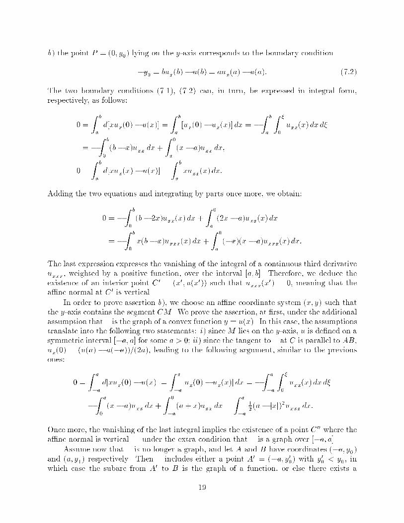
b) the point P = (0; y0) lying on the y-axis corresponds to the boundary condition

�y0 = bux(b) � u(b) = aux(a) � u(a): (7:2)

The two boundary conditions (7.1), (7.2) can, in turn, be expressed in integral form,

respectively, as follows:

0 =

Z b

a

d[xux(0) � u(x)] =

Z b

a

[ux(0)� ux(x)] dx = �Z b

a

Z �

0

uxx(x) dx d�

= �Z b

0

(b � x)uxx dx+

Z 0

a

(x � a)uxx dx;

0 =

Z b

a

d[xux(x) � u(x)] =

Z b

a

xuxx(x) dx:

Adding the two equations and integrating by parts once more, we obtain:

0 = �Z b

0

(b� 2x)uxx(x) dx +

Z 0

a

(2x � a)uxx(x) dx

= �Z b

0

x(b � x)uxxx(x) dx +

Z 0

a

(�x)(x � a)uxxx(x) dx:

The last expression expresses the vanishing of the integral of a continuous third derivativeuxxx, weighted by a positive function, over the interval [a; b]. Therefore, we deduce theexistence of an interior point C 0 = (x0; u(x0)) such that uxxx(x

0) = 0, meaning that thea�ne normal at C 0 is vertical.

In order to prove assertion b), we choose an a�ne coordinate system (x; y) such thatthe y-axis contains the segment CM . We prove the assertion, at �rst, under the additionalassumption that � is the graph of a convex function y = u(x). In this case, the assumptionstranslate into the following two statements: i) sinceM lies on the y-axis, u is de�ned on asymmetric interval [�a; a] for some a > 0; ii) since the tangent to � at C is parallel to AB,

ux(0) = (u(a) � u(�a))=(2a), leading to the following argument, similar to the previous

ones:

0 =

Z a

�a

d[xux(0) � u(x)] =

Z a

�a

[ux(0) � ux(x)] dx = �Z a

�a

Z �

0

uxx(x) dx d�

= �Z a

0

(x � a)uxx dx +

Z 0

�a

(a + x)uxx dx =

Z a

�a

12(a � jxj)2uxxx dx:

Once more, the vanishing of the last integral implies the existence of a point C 00 where thea�ne normal is vertical | under the extra condition that � is a graph over [�a; a].

Assume now that � is no longer a graph, and let A and B have coordinates (�a; y0)and (a; y1) respectively. Then � includes either a point A0 = (�a; y00) with y00 < y0, in

which case the subarc from A0 to B is the graph of a function, or else there exists a

19

MA B

C

A’ B’

Figure 5. Mean A�ne Normal.

point B0 = (a; y01) with y01 < y1, in which case the subarc from A to B0 is the graph of afunction (but not both, since � is a short arc). Without loss of generality, we assume theformer case, as in Figure 5. In this case, a vertical line drawn downwards (i.e., in the samedirection as MC) from A meets � at another point A0, and a line from A0 in the directionof AB (i.e., to the right) meets � at a point B0. It is clear that the midpoint M 0 of thesegment A0B0 is to the left of the segment CM . Therefore, replacing � by the subarc �0

from A0 to B0, one may apply the previous argument, whereby there is a point in �0 wherethe a�ne normal is in the same direction as CM 0, that is to say to the left of CM . Onthe other hand, the arc of � from A to A0, by a similar argument, contains a point wherethe a�ne normal points to the right of the direction of A0A, or, equivalently, CM . Bycontinuity, there exists a point C 00 in the subarc of � from A to B0 where the a�ne normalis in the same direction as CM . This concludes the proof of Theorem 7.2. Q.E.D.

A somewhat di�erent geometrical construction of mean a�ne normals for a shortconvex arc is described by the following theorem.

Theorem 7.3. Let � be a short, smooth, convex arc, inscribed in the triangle

T = APB, as above, and let M be the midpoint of the chord AB. For any point C 2 �,not an end point, denote by PA and PB the points of intersection of the tangent to � at Cwith the segments PA and PB, respectively. Then there exists at least one point C 2 �

which is the midpoint of the associated segment PAPB. Furthermore, for any such point,

there exist points C 0; C 00 2 � where the a�ne normal is in the same direction as PC orCM , respectively.

Proof : To show the existence of the point C, consider the area of the triangle PAPPBas C varies between A and B. The area is always positive, continuously dependent on C,and approaches zero as C approaches either A or B. The desired point C occurs whenthis area attains a (local) maximum value. Note that if � were to include a sub-arc �0 ofa hyperbola having PA and PB as asymptotes, then each point C 2 �0 would have the

desired property.

20

Assuming, then that C is the midpoint of its associated segment PAPB, we proceed to

prove, �rst, that the direction PC occurs as a direction of an a�ne normal to �. Let (x; y)be an a�ne coordinate system such that the y-axis contains the segment PC with the same

orientation. The assumptions imply, �rst of all, that � is the graph of a convex function

y = u(x) de�ned over a closed interval a � x � b withe a < 0 < b. The assumptions that

P lies on the y-axis is equivalent to the boundary condition (7.2). It is now convenient tochoose the direction of the x-axis to be parallel to PAPB, which means that ux(a) = �ux(b)and ux(0) = 0. Our assumption that C is the midpoint of PAPB means that

ux(b) � 2ux(0) + ux(a) = 0: (7:3)

We now introduce a Legendre transform of the function u: choose the strictly mono-

tone function ux(x) � ux(0) of x as the new independent variable x and the transformed

function y = u(x) = xux(x) � u(x) as the new dependent variable. Then

dx = uxx dx; dy = xuxx dx = xdx:

Therefored2u

dx2=

1

uxx> 0:

The boundary condition (7.3), in terms of the transformed function, sets the interval ofde�nition of u to be [�a; a], where a = ux(b)�ux(0) = ux(0)�ux(a), while (7.2) becomesu(�a) = u(a). In addition, we have ux(0) = 0. These conditions on the transformedvariables and the function u include the properties of the function u in the proof of assertionb) of Theorem 7.2, namely the graph b� of u, with end points bA = (�a; u(�a)), bB =

(a; u(a)), and the point bC = (0; u(0)) such that 2au(0) = u(a) � u(�a) (both sides herebeing zero). Therefore there exists an intermediate value x0 corresponding to x0 = ux(x

0) 2[a; b], for which uxxx(x

0) = �uxxx(x0)=[uxx(x0)]2 = 0. This shows the existence of C 0 =(x0; u(x0)) 2 � where the a�ne normal is in the same direction as PCy.

To show the existence of a point C 00 2 � whose a�ne normal is in the same directionas CM , we arrange the y axis of our equia�ne coordinate system to include the segmentCM in the positive direction, as in Figure 6. Introduce the chords AC and CB, and let

MA andMB be their respective midpoints, such that the corresponding a�ne normals arepositive scalar multiples of the vectors MA �PA and MB �PB respectively. On the otherhand, taking into account the identities

MA � PA = 12(A� PA) +

14(PB � PA); MB � PB = 1

2(B � PB) +

14(PA � PB);

y It is possible, of course, to give the same proof without using Legendre transforms; howeverthe steps to deduce, by two integrations by parts, from the assumptions on u the correspondingidentity

0 =

Z b

adu(x) =

1

2

Z b

a

hux(b) � ux(0)� jux(x)� ux(0)j

i2 uxxx

(uxx)2dx

would seem much more opaque than the proof presented here.

21

A

B

P

C

PA

PB

MA

MB

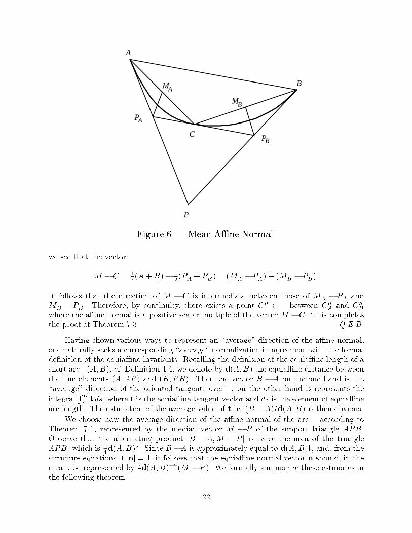
Figure 6. Mean A�ne Normal.

we see that the vector

M � C = 12(A+B) � 1

2(PA + PB) = (MA � PA) + (MB � PB):

It follows that the direction of M � C is intermediate between those of MA � PA andMB � PB . Therefore, by continuity, there exists a point C 00 2 � between C 00

A and C 00B

where the a�ne normal is a positive scalar multiple of the vector M �C. This completesthe proof of Theorem 7.3. Q.E.D.

Having shown various ways to represent an \average" direction of the a�ne normal,one naturally seeks a corresponding \average" normalization in agreement with the formal

de�nition of the equia�ne invariants. Recalling the de�nition of the equia�ne length of ashort arc �(A;B), cf. De�nition 4.4, we denote by d(A;B) the equia�ne distance betweenthe line elements (A;AP ) and (B;PB). Then the vector B � A on the one hand is the

\average" direction of the oriented tangents over �; on the other hand it represents the

integralRBAt ds, where t is the equia�ne tangent vector and ds is the element of equia�ne

arc length. The estimation of the average value of t by (B �A)=d(A;B) is then obvious.

We choose now the average direction of the a�ne normal of the arc � according to

Theorem 7.1, represented by the median vector M � P of the support triangle APB.

Observe that the alternating product [B � A;M � P ] is twice the area of the triangleAPB, which is 1

4d(A;B)3. Since B�A is approximately equal to d(A;B)t, and, from the

structure equations [t;n] = 1, it follows that the equia�ne normal vector n should, in the

mean, be represented by 4d(A;B)�2(M � P ). We formally summarize these estimates inthe following theorem.

22

Theorem 7.4. Let � be a short arc and let d(A;B) be the equia�ne distance

between its endpoints A and B, i.e., twice the cube root of the area of its support triangleAPB. Let M be the midpoint of the chord AB. Then a mean value for the equia�ne

frame (t;n), consisting of the tangent and normal to �, is represented by

tav =B �A

d(A;B); nav = 4

M � P

d(A;B)2:

8. The A�ne Curvature.

The structure equation (6.2) has two obvious consequences that serve to interpret

it in geometrical terms. In the �rst place, under in�nitesimal displacements of a pointon the curve, the equia�ne normal shifts parallel to the tangent. Secondly, the sign of

the equia�ne curvature � tells us which way the a�ne normal varies over small arcs of

a convex curve. More precisely, if � is everywhere positive in a short arc, then the a�nenormals at its endpoints, both pointing into the concave side of the curve, lean towardseach other, like the Euclidean normals of a convex arc, while if � < 0 everywhere, then thea�ne normals lean away from each other. One can apply the results of the last section tomake these statements more precise.

Proposition 8.1. Let � be a short arc of a smooth, convex curve, and let APBbe its support triangle. Let C 2 � be the point whose tangent line is parallel to thechord AB, and let the tangent line at C intersect the segments PA and PB at PA andPB respectively. Let t = tA;B be the real number, 0 < t < 1 de�ned by the equivalentvector relations PA � P = t(A � P ) or PB � P = t(B � P ). Then there exists a point on� where the equia�ne curvature � is positive, negative, or zero according to whether t is,respectively, > 1

2, or < 1

2, or = 1

2.

Proof : We refer to Figure 7. Draw the chords of � from A to C and from C to B, andlet MA andMB be their respective midpoints. It follows that the vector MB �MA equals12(B � A). Since the tangent at C is parallel to the line AB, it follows that PB � PA =

t(B �A), where t is as in the statement of the proposition. From Theorem 7.1 we knownthat the directed half-lines PAMA and PBMB represent mean directions of the equia�ne

normal in the respective portions of �. To compare these two directions, one immediately

veri�es that

(MB � PB) � (MA � PA) = (MB �MA) � (PB � PA) = (12� t)(B �A):

The required conclusion now follows. Q.E.D.

Corollary 8.2. Let � be a smooth, closed, convex curve without in ection points inthe a�ne plane. Let B denote the convex body bounded by �. Let B� denote the convexbody neighborhood of B, obtained as the Minkowski sum B

� = 2B+ (�B).y Then, from

every point on the boundary of B� (and, a fortiori from every exterior point of B�) onecan \see" at least one point on � where the equia�ne curvature is positive.

y In other words, B� is the set of points P for which one can �nd points M;Q 2 B such that

M is the midpoint of the segment PQ.

23

A

B

P

CPA

PB

MAMB

Y

Figure 7. A�ne Curvature Construction.

Remark : This statement is considerably stronger than one found in various textbooks,asserting the existence of a point with positive equia�ne curvature on any \half-oval", i.e.,on any locally convex, smooth bounded arc whose tangents at the endpoints are parallel,and with no other pair of parallel tangents.

Proof : Let P be any point on the boundary of B�, and let PA and PB be the twotangent lines to � from P , where A and B are the respective points of contact with �. LetA0 and B0 be the midpoints of the respective segments PA and PB. It follows from thede�nition of B� that the line A0B0 cannot meet B. Consequently, if one draws the tangentline to the short arc of � between A and B, i.e., the set of points of � that are visible from

P , then the ratio tA;B de�ned in Proposition 8.1 is strictly greater than 12. Q.E.D.

To conclude this section, we shall re�ne the last proposition to yield a numericalapproximation to the actual value of the equia�ne curvature of a short arc.

Theorem 8.3. Let � be a short arc of a smooth, convex curve, with end points

A, B, and the same construction as in Proposition 8.1. Let d(A;B) denote the equia�nedistance from A to B. In Figure 6, prolong the lines PAMA and PBMB to their intersection

point Y (if necessary, in the projective completion of the plane), as depicted in Figure 8.The three points P , C, and Y lie on a common line. Let QC denote the intersection of

that line with the chord AB, and consider the (negatively valued) cross ratio

�(A;B) = [QC ; P : Y;C] =(QCY : PY )

(QCC : PC):

24

A

B

P

C

PA

PB

MAMB

Y

QAQB

QC

Figure 8. Equia�ne Curvature Approximation.

Then a mean value of the equia�ne curvature � over � is represented by

�� = 81 + �(A;B)

d(A;B)2: (8:1)

Proof : The collinearity of the three points P , C, and Y follows from Desargues'Theorem. From the perspective point A, the four points P , C, QC , Y , de�ning the crossratio �, may be projected to the corresponding points PA, MA, QA, Y in the line PAMA.

(Equivalently, we can project from B to obtain PB, MB , QB , Y in the line PBMB .) SinceMA is the midpoint of PAQA, the cross ratio � reduces to the scalar coe�cient in the linearvector relation Y �QA = ��(Y � PA), whence

MA � PA = 12(1 + �)(Y � PA): (8:2)

According to Theorem 7.4,

MA � PA = 14d(A;C)2n(A;C); (8:3)

where d(A;C) is twice the cube root of the area of the triangle APAC (and asymptot-ically the a�ne length of the arc AC in �) and n(A;C) is a mean vector value of the

equia�ne normal over the same arc. Furthermore, the point Y , marking the intersectionof two neighboring a�ne normal lines, approximates, as the arc � is shortened to a point

25

X 2 �, the corresponding point X + ��1n of the a�ne evolute of � at X. Combining the

approximate relations Y �PA � ��1n(A;C) with (8.3), we see from (8.2) that an approx-imate value � of the equia�ne curvature is given by 1

8(1 + �)d(A;C)�2. Interchanging A

and B, we have another approximation � � 12(1 + �)d(C;B)�2. Recalling Theorem 4.3,

the equia�ne length of � is approximated by d(A;B), or, alternatively, by 2d(A;C) or

2d(C;B). Combining these formulas completes the proof of (8.1). Q.E.D.

Although (8.1) can in principle be used as a method for approximating the a�ne

curvature, it has several numerical di�culties that preclude its direct use. First, the

construction relies on the introduction of the tangent lines at the point A and B, and hence

we need to introduce an additional numerical approximation. Moreover, the approximationneeds to incorporate a�ne invariances, and so the standard di�erence quotient is not

satisfactory for this purpose. More serious is the instability in the computation of the

intersection point Y , which can be at in�nity (and indeed is if the curve is a parabola),and is thus highly unstable from a numerical point of view. Presumably, one can overcomethe latter di�culty by mutliplying the numerator and denominator in the ratio (8.1) byan appropriate factor, although we have not thoroughly investigated this as of yet.

9. Finite Di�erence Approximations of A�ne Invariants.

In this section, we discuss a fully a�ne-invariant �nite di�erence approximation to thea�ne curvature of a convex curve in the plane. The starting point is the result that onecan approximate the (positive) a�ne curvature at a point of a plane curve by the a�necurvature of the conic section passing through �ve nearby points. We will explicitly showhow this may be used to produce an a�ne-invariant �nite di�erence approximation to thea�ne curvature. The �rst item is to determine the formula for the a�ne curvature of aconic passing through �ve points.

Given a numbered set of points Pi, i = 0; 1; 2; : : :, we let

[ijk] = [Pi; Pj ; Pk] = (Pi � Pj) ^ (Pi � Pk)

denote twice the (signed) area of the triangle with vertices Pi; Pj ; Pk, cf. (3.2). See [23],[28], for a proof of the following elementary fact.

Theorem 9.1. Let P0; : : : ; P4 be �ve points in general position in the plane. Thereis then a unique conic section C passing through them, whose quadratic equation has thea�ne-invariant form

[013][024][x12][x34] = [012][034][x13][x24]; (9:1)

where x = (x; y) is an arbitrary point on C.In order to compute the a�ne curvature of the conic (9.1), we use formula (6.5), and

thus need to compute the two equia�ne invariants S, T , as given in (6.6), in equia�ne

invariant form. In other words, the resulting formula should be written in terms of the

26

P0

P1

P2

P3

P4

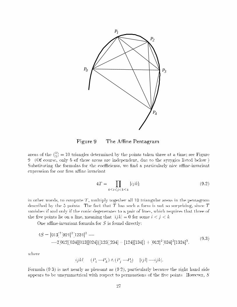
Figure 9. The A�ne Pentagram.

areas of the�5

3

�= 10 triangles determined by the points taken three at a time; see Figure

9. (Of course, only 5 of these areas are independent, due to the syzygies listed below.)Substituting the formulas for the coe�cients, we �nd a particularly nice a�ne-invariantexpression for our �rst a�ne invariant

4T =Y

0�i<j<k�4

[ijk]; (9:2)

in other words, to compute T , multiply together all 10 triangular areas in the pentagramdescribed by the 5 points. The fact that T has such a form is not so surprising, since Tvanishes if and only if the conic degenerates to a pair of lines, which requires that three of

the �ve points lie on a line, meaning that [ijk] = 0 for some i < j < k.

One a�ne-invariant formula for S is found directly:

4S = [013]2[024]2[1234]2 �� 2[012][034][013][024]

�[123][234] + [124][134]

�+ [012]2[034]2[1324]2:

(9:3)

where

[ijkl] = (Pi � Pk) ^ (Pj � Pl) = [ijl]� [ijk]:

Formula (9.3) is not nearly as pleasant as (9.2), particularly because the right hand side

appears to be unsymmetrical with respect to permuations of the �ve points. However, S

27

must clearly be symmetrical with respect to these permutations. Of course, the explanation

lies in the syzygies among the triangular areas: these are

[123] = [012] + [023] + [031]; (9:4)

[012][034]� [013][024] + [014][023] = 0; (9:5)

and the analogous formulas obtained by permutation of the symbols 0; : : : ; 4, cf. (2.5), (2.6).

A judicious application of (9.4), (9.5), will su�ce to demonstrate that (9.3) is symmetricalunder permutation. A completely symmetrical formula for S can, of course, be obtained

by symmetrizing (9.3), i.e., summing over all possible permutations of the set f0; 1; 2; 3; 4gand dividing by 5! = 120, although the result is much more complicated than (9.3). We

have been unable to �nd a simple yet symmetrical version of the formula for S.

As in the Euclidean case, we are interested in numerical approximations to the a�necurvature of a strongly convex plane curve � which are invariant under the special a�negroup. As before, we approximate the parametrized curve x(r) = (x(r); y(r)) by a sequenceof mesh points Pi = x(ri). Any a�ne-invariant numerical approximation to the a�necurvature � (as well as any other a�ne di�erential invariant dn�=dsn) must be a functionof the joint a�ne invariants of the mesh points, which means that it must be a functionof the areas [ijk] = [PiPjPk] of the parallelograms (or triangles) described by the meshpoints. Because the a�ne curvature is a fourth order di�erential function, the simplestapproximation will require �ve mesh points, so that the approximation will depend onthe ten triangular areas (or, more basically, the �ve independent areas) in the pentagramwhose vertices are the �ve mesh points; see Figure 9.

With this in mind, let us number the �ve successive mesh points as P0; P1; P2; P3; P4.(This is just for simplicity of exposition; of course, in general, one should replace theindices 0; : : : ; 4 by i; i + 1; i + 2; i + 3; i + 4.) Since we are assuming that � is convex,the mesh points are in general position. Let C = C(P0; P1; P2; P3; P4) be the unique conicpassing through the mesh points. Let e� = e�(P0; P1; P2; P3; P4) denote the a�ne curvatureof the conic C, which we evaluate via the basic formula (6.5), where the invariants S, T

are computed in terms of the triangular areas according to (9.3), (9.2). We regard e� as anumerical approximation to the a�ne curvature � = �(P2) of � at the middle point P2. Wenow need to analyze how closely the numerical approximation e� is to the true curvature� at the point P2. Assuming the points are close together (see the discussion below), we

need to compute a Taylor series expansion of the distance e�. An extensive Mathematica

computation produces the desired result

Theorem 9.2. Let P0; P1; P2; P3; P4 be �ve successive points on the convex curve

�. Let � be the a�ne curvature of � at P2, and let e� denote the a�ne curvature of the

conic section passing through the �ve points. Let

Li =

Z Pi

P2

ds; i = 0; : : : ; 4; (9:6)

28

denote the signed a�ne arc length of the conic from P2 to Pi; in particular L2 = 0. We

assume that each Li is small. Then the following expansion is valid:

e� = �+1

5

4Xi=0

Li

!d�

ds+

1

30

0@ X

0�i�j�4

LiLj

1A d2�

ds2+ � � � : (9:7)

The higher order terms are cubic in the distances Li.

Remark : The property of \being close" is therefore expressed in a�ne-invariant form

as the statement that all the arc lengths L0; : : : ; L4 are small. In this way, we are able to

introduce a fully a�ne-invariant notion of \distance", albeit one that requires knowledgeof �ve, rather than two, points.

Proof : This is found by a direct Taylor series expansion of the a�ne-invariant expres-sions (9.3), (9.2), for the a�ne invariants S, T , and then substitution into the formula (6.5)for the curvature of the conic section. We represent the curve as the graph of y = u(x),which, assuming the three points are su�ciently close, can always be arranged. The pointscan be assumed to be P0 = (h; u(h)), P1 = (i; u(i)), P2 = (0; 0) = (0; u(0)), P3 = (j; u(j)),P4 = (k; u(k)), where h; i; j; k are small. The areas are then given, for example, by

[013] = (h � i)(u(h) � u(j))� (h� j)(u(h)� u(i)) = hu(i)� iu(h)� hu(j) + ju(h);

with elementary Taylor series expansion. The result is a Taylor series expansion for e� interms of h; i; j; k, with leading term �, as given in (6.2), the derivatives being evaluatedat 0. However, h; i; j; k, being the di�erences of the x coordinates of the mesh points, arenot a�ne invariant, and hence the coe�cients of the expansion are not a�ne di�erentialinvariants. To remedy this, we must introduce the a�ne arc lengths (9.6) as our basica�ne-invariant paramaters. Using the formula (6.3) for the a�ne-invariant arc lengthelement, the expansion

L0 =

Z h

0

3

puxx dx = h 3

puxx +

16h2

uxxx(uxx)

2=3+ � � � ; (9:8)

can be inverted to produce a Taylor series expressing h in terms of L0. Plugging this,and the analogous series for i; j; k into the previous Taylor series produces the �nal re-sult. Q.E.D.

Remark : An a�ne invariant �nite di�erence approximation to the a�ne normal canalso be found by computing the a�ne normal to the approximating conic C at the middlepoint P2, and expressing this in terms of the triangular areas. The method can also produceinvariant numerical methods for computing d�=ds, etc., using more points.

10. A General Conjecture.

The reader has probably already noticed that the Euclidean and a�ne curvature ap-

proximation series (3.9), (9.7), bear a remarkable similarity. This suggests a generalization

29

which we indicate here, albeit as a conjecture without proof. We begin by surveying the

general theory of di�erential invariants of �nite-dimensional Lie groups of transformationsin the plane; see [17] for a detailed presentation. Let G be an r-dimensional Lie group

acting on E = 2, with coordinates x; y, and let g denote its Lie algebra of in�nitesimal

generators, which are vector �elds v = �(x; y)@x + �(x; y)@y on E. Curves in the plane

are then (locally) represented as functions y = u(x). Let Jn denote the nth jet space ofE, which has coordinates (x; u(n)) = (x; u; ux; uxx; : : : ; un). There exists a G-invariant arc

length element dsG = P (x; u(n)) dx represented by the simplest (lowest order) G-invariant

one-form, and a G-invariant curvature �G, which is the simplest (lowest order) di�erential

invariant. We also assume that G determines an \ordinary" action, meaning that it acts

transitively and locally e�ectively on E, and, moreover, its prolonged actions G(n)are alsolocally transitive on a dense open subset of Jn for all 0 � n � r� 2, where r is the dimen-

sion of G. (In the language of [17], G admits no pseudo-stabilization of the prolonged orbit

dimensions.) Indeed, Lie's complete classi�cation of all �nite-dimensional transformationgroups on the plane, [15], [17], shows that, of the transitive groups, only the elementarysimilarity group (x; u) 7! (�x + c; �u + d) and some minor variants thereof fail this hy-pothesis. Under these assumptions, the G-invariant arc length has order n � r�2 and theG-invariant curvature �(x; u(r�1)) has order exactly r � 1. The solutions to the ordinarydi�erential equation

�(x; u(r�1)) = c; (10:1)

for c constant determine the curves of constant curvature for the group action. In fact,one does not need to integrate the ordinary di�erential equation (10.1), since these curvescan be found directly from the group action.

Proposition 10.1. A curve � �M has constant G-invariant curvature if and onlyif it is the orbit, � = exp(tv)P0, of some point P0 2 M under a one-parameter subgroupexp(tv) � G determined by an in�nitesimal generator v 2 g.

Thus, for the Euclidean group, we recover the circles and straight lines as the constantcurvature curves, while for the special a�ne group, these are the conic sections. Since (10.1)has order r � 1, given r points P1; : : : ; Pr 2 E in \general position", there exists a unique

constant curvature curve �0(P1; : : : ; Pr) passing through them. Let �0(P1; : : : ; Pr) denoteits curvature. Since (10:1) is a G-invariant ordinary di�erential equation, �0(P1; : : : ; Pr)is a joint invariant of the r points.

Let � � M be an arbitrary curve in the plane. We are interested in constructing aG-invariant �nite di�erence approximation to its G-invariant curvature �(P1) at a given

point P1 2 � in the curve. Choose r� 1 nearby points P2; : : : ; Pr 2 �. Then the curvature�0 = �0(P1; : : : ; Pr) of the constant curvature curve �0 = �0(P1; : : : ; Pr) passing through

the points determines our approximation to �(P1).

Conjecture: The following series expansion holds:

�0 = �+1

r

rXi=1

Li

!d�

ds+

1

r(r + 1)

0@ X

1�i�j�r

LiLj

1A d2�

ds2+ � � � ; (10:2)

30

where �, d�=ds, etc. are evaluated at P1, and

Li =

Z Pj

P1

ds; (10:3)

denotes the G-invariant \distance" from the point P1 to Pj, measured as the G-invariant

arc length along the constant curvature curve �0. (In particular, L1 = 0.) The expansion

assumes that all the arc lengths Li are small.

Example 10.2. Consider the translation group (x; u) 7! (x+ c; u+d). In this case,� = du=dx, and the constant curvature curves are the straight lines. Then �0(p1; p2) =

(u2 � u1)=(x2 � x1). Therefore, the expansion (10.2) is merely the Taylor series, and so

is valid to general order! (Note that since dx is the translation-invariant arc length, the

\length" of a straight line segment isR P2P1

dx = x2 � x1.)

Thus, the conjectured series expansion (10.2) is valid up to order 2 for the translationgroup, the Euclidean group, and the special a�ne group. Direct veri�cation for otherplanar groups appears to be problematic because the formulas for the �nite di�erenceapproximation �0 are not so easy to come by, because the constant curvature curves involvetranscendental functions. Moreover, preliminary computations with the Euclidean groupindicate that the natural generalization of (10.2) is not valid to order 3. Thus, the seriesshould be viewed perhaps more as an interesting speculation rather than a �rm conjecture.

11. A�ne Curvature Flow.

In this section, we will present several new solutions to an a�ne invariant nonlinearheat equation which arose out of certain problems in vision and image processing. Indeed,invariant theory has recently become a major topic of study in computer vision. Sincethe same object may be seen from a number of points of view, one is motivated to lookfor shape invariants under various transformations. A closely related topic that has beenreceiving much attention from the image analysis community is the theory of scale-spaces

or multiscale representations of shapes for object recognition and representation; see [12]for an extensive list of references on the subject. Initially, most of the work was devotedto linear scale-spaces derived �ltering using a Gaussian kernel or equivalently running the

shapes through the linear heat equation. Here the variance of the �lter (or equivalently

the time of the heat equation) plays the role of a scale-space parameter. The greater thevariance (or time), the more the given shape is smoothed. Of course, the di�usion beingisotropic, the shape will be blurred as well. To remedy such problems, in the last fewyears, a number of non-linear and geometric scale-spaces have been investigated as well.

The idea is to introduce a nonlinear smoothing which preserves edges while smoothing oneither side of the edge. Such nonlinear smoothing methods may be found in [21], [4], and

[13]. See also the references in [12]. The combination of invariant theory and geometricmultiscale analysis was investigated in [24] and [25]. There, the authors introduced an

a�ne invariant geometric scale-space. Part of this work was extended to other groupsas well in [18], [19]; see also [4]. The shape representations which we derive allow us

31

to compute invariant signatures at di�erent scales and in a robust way. These ows are

already being used with satisfactory results in various applications [12].

The a�ne curvature ow was introduced precisely to give an a�ne invariant multiscale

representation of planar shape. For closed convex curves, the a�ne curvature ow is

found by evolving the curve in the direction of its a�ne normal, proportional to the a�ne

curvature, and so has the form

xt = �n; (11:1)

where � is the a�ne curvature and n the a�ne normal. Interestingly, although the a�necurvature depends on fourth order derivatives of the parametrized curve, we can replace

(11.1) by a much simpler ow whose image curves are the same, di�ering only by an

inessential reparametrization. Speci�cally, we rewrite the a�ne normal n in terms of the

tangential and Euclidean normal directions to the curve, leading to an evolutionary owof the form

xt =3

p�e ne + F t; (11:2)

where �e is the Euclidean curvature, ne the Euclidean (inward) normal, and F is somefunction of the curvature and its derivatives whose precise form is irrelevant. Indeed,since the tangential component F t in (11.2) only a�ects the reparametrization of theimage curve, this term can be safely omitted (or even replaced by any other convenient

tangential term eF t if desired). As a result, the ow (11.1) can be written in the equivalent(but non-a�ne-invariant) form

xt =3

p�e ne: (11:3)

Note that, in the form (11.3), the ow can be extended to nonconvex curves | in ectionpoints have zero Euclidean curvature, but that does not cause any di�culties for eitherthe Euclidean normal or curvature, even though the a�ne curvature is not well de�ned atsuch points. In particular, if the curve is given as the graph of a function y = u(x), thenthe normal version (11.3) of the a�ne curvature ow has the particularly simple form

ut =3

puxx : (11:4)

An alternative, useful formulation of the a�ne ow is obtained by taking the cross

product of (11.2) with the tangent vector xr to the parametrized curve x(r; t) at timet. Using the formula (3.4) for the Euclidean curvature of a parametrized curve x(r) =(x(r); y(r)), and the fact that xr ^ ne = jxrj2, we �nd that the components x(r), y(r) of

x must satisfy the underdetermined second order partial di�erential equation

(xr ^ xt)3 = xr ^ xrr ; or (xryt � xtyr)3 = xryrr � xrryr : (11:5)

Conversely, since xr is parallel to the unit tangent vector t, given a solution to (11.5),it must also satisfy (11.2) for some choice of tangential component F t, and hence theindividual image curves for each value of t will describe solution to the a�ne curvature

ow (11.1) (although they will not necessarily have the correct parametrization to satisfy

the normal version (11.3)).

32

Figure 10. Quintic Fan.

Very few nontrivial particular solutions to the a�ne curvature ow are known. First,the curves of constant a�ne curvature will evolve analogously to the Euclidean circles.Thus, an initial ellipse will remain elliptical, having the same eccentricity and orientation,while collapsing to a point. Moreover, recent results of Angenent, Sapiro, Tannenbaum,[5], demonstrate a smooth closed embedded curve remains regular, eventually shrinking toa point.

There is an a�ne analogue of the grim reaper. If we choose the vertical axis to

translate along, the solution is obtained by setting ut = c, for constant c in (11.4). Theresult is a vertically translating parabolic solution

y = u(x; t) = 12c3(x� x0)

2 + c(t� t0): (11:6)

We have also constructed some examples of solutions having in ection points. Thesimplest example is found by assuming ut = cx in (11.4). Omitting an inessential integra-

tion constant, the resulting solution is

y = u(x; t) = 120c3x5 + ctx;

which, at each value of t, has a stationary in ection point at the origin. The successiveimage curves of the \quintic fan" are depicted in Figure 10.

To produce explicit solutions with non-stationary in ection point is more di�cult.

The following procedure allows us to describe another solution having a moving in ection

33

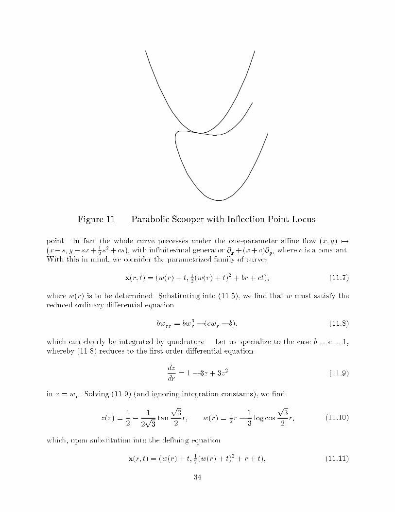
Figure 11. Parabolic Scooper with In ection Point Locus.

point. In fact the whole curve precesses under the one-parameter a�ne ow (x; y) 7!(x+ s; y+ sx+ 1

2s2+ cs), with in�nitesimal generator @x+(x+ c)@y, where c is a constant.

With this in mind, we consider the parametrized family of curves

x(r; t) = (w(r) + t; 12(w(r) + t)2 + br + ct); (11:7)

where w(r) is to be determined. Substituting into (11.5), we �nd that w must satisfy thereduced ordinary di�erential equation

bwrr = bw3r � (cwr � b); (11:8)

which can clearly be integrated by quadrature. Let us specialize to the case b = c = 1,

whereby (11.8) reduces to the �rst order di�erential equation

dz

dr= 1� 3z + 3z2 (11:9)

in z = wr. Solving (11.9) (and ignoring integration constants), we �nd

z(r) =1

2+

1

2p3tan

p3

2r; w(r) = 1

2r � 1

3log cos

p3

2r; (11:10)

which, upon substitution into the de�ning equation

x(r; t) = (w(r) + t; 12(w(r) + t)2 + r + t); (11:11)

34

Figure 12. Parabolic Scooper.

produces the desired solution. The curve looks like a version of the Euclidean grim reaper,but bent around a parabola. It has a triple in ection point on the interior half of thecurve, close to the point of maximum curvature. Since xr ^xrr = 0 at the in ection point,it is explicitly given by solving z = wr = 1, so that r = 2�=3

p3. Thus, the in ection point

traces out a parabola

y = 12x2 + x +

�

3p3� 1

3log 2;

see Figure 11 for a picture of the curve (at t = 0) and the parabolic locus traced out by

the in ection points. The actual curve evolution, which we propose to call the \parabolicscooper" is depicted in Figure 12; notice the in ection parabola reappearing as an envelopeto the curve family.

An important point of interest of this example is that it describes the asymptotic be-havior in the small of any (triple) in ection point that is precessing. Indeed, translating thein ection point for t = 0 to the origin, one �nds the following convenient reparametrization

x(r) = �Z

dr

1 + r3= �r + 1

4r4 � � � � ;

y(r) =1

2x(r)2 �

Zrdr

1 + r3= � 1

20r5 +

11

112r8 � � � � ;

clearly demonstrating the nature of the in ection point.

Finally, for numerical implementations of the a�ne ow based on the Osher-Sethian

level curve algorithm [20] as well as explicit applications to invariant planar curve rep-resentation, see [25]. Implementations based on the applications of our a�ne-invariant

35

�nite di�erence approximations are under development, and will form the subject of a

subsequent work.

References

[1] Ackerman, M., and Hermann, R., Sophus Lie's 1880 Transformation Group Paper,

Math Sci Press, Brookline, Mass., 1975.

[2] Ackerman, M., and Hermann, R., Sophus Lie's 1884 Di�erential Invariant Paper,

Math Sci Press, Brookline, Mass., 1976.

[3] Alvarez, L., Lions, P.L., and Morel, J.M., Image selective smoothing and edge

detection by nonlinear di�usion, SIAM J. Numer. Anal. 29 (1992), 845{866.

[4] Alvarez, L., Guichard, F., Lions, P.L., and Morel, J.M., Axioms and fundamentalequations of image processing, Arch. Rat. Mech. 123 (1993), .

[5] Angenent, S., Sapiro, G., and Tannenbaum, A., On the a�ne invariant heatequation for nonconvex curves, preprint, in preparation.

[6] Blaschke, W., Vorlesungen �uber Di�erentialgeometrie, Vol. II, J. Springer, Berlin,1923.

[7] Dorodnitsyn, V.A., Transformation groups in net spaces, J. Sov. Math. 55 (1991),1490{1517.

[8] Dorodnitsyn, V.A., Symmetry of �nite di�erence equations, in: CRC Handbook of

Lie Group Analysis of Di�erential Equations, Vol. 1, Ibragimov, N.H., ed., CRCPress, Boca Raton, Fl., 1994, pp. 349{403.

[9] Gage, M., and Hamilton, R.S., The heat equation shrinking convex plane curves, J.Di�. Geom. 23 (1986), 69{96.

[10] Grayson, M., The heat equation shrinks embedded plane curves to round points, J.Di�. Geom. 26 (1987), 285{314.

[11] Green, M.L., The moving frame, di�erential invariants and rigidity theorems forcurves in homogeneous spaces, Duke Math. J. 45 (1978), 735{779.

[12] ter Haar Romeny, B. (editor), Geometry Driven Di�usion in Computer Vision,Kluwer, Holland, 1994.

[13] Kimia, B, Tannenbaum, A., and Zucker, S., On the evolution of curves via afunction of curvature, J. Math. Anal. Appl. 163 (1992), 438{458.

[14] Li, A.{M., Simon, U., and Zhao, G., Global A�ne Di�erential Geometry of

Hypersurfaces, W. de Gruyter, New York, 1993.

[15] Lie, S., Theorie der Transformationsgruppen I, Math. Ann. 16 (1880), 441{528; alsoGesammelte Abhandlungen, Vol. 6, B.G. Teubner, Leipzig, 1927, pp. 1{94; see

[1] for an English translation.

[16] Lie, S., �Uber Di�erentialinvarianten, Math. Ann. 24 (1884), 537{578; alsoGesammelte Abhandlungen, Vol. 6, B.G. Teubner, Leipzig, 1927, pp. 95{138; see

[2] for an English translation.

36

[17] Olver, P.J., Equivalence, Invariants, and Symmetry, Cambridge University Press,

1995.

[18] Olver, P.J., Sapiro, G., and Tannenbaum, A., Classi�cation and uniqueness of

invariant geometric ows, Comptes Rendus Acad. Sci. (Paris), S�erie I, 319

(1994), 339{344.

[19] Olver, P.J., Sapiro, G., and Tannenbaum, A., Di�erential invariant signatures and ows in computer vision: a symmetry group approach, in: Geometry{Driven

Di�usion in Computer Vision, B. M. Ter Haar Romeny, ed., Kluwer Acad.

Publ., Dordrecht, the Netherlands, 1994, pp. 205{306.

[20] Osher, S., and Sethian, J., Front propagation with curvature dependent speed:

Algorithms based on Hamilton-Jacobi formulations, Journal of Computational

Physics 79 (1988), 12{49.

[21] Perona, P., and Malik, J., Scale-space and edge detection using anisotropic di�usion,

IEEE PAMI 12 (1990), 629{639.

[22] Salkowski, E., A�ne Di�erentialgeometrie, W. de Gruyter, Berlin, 1934.

[23] Salmon, G., A Treatise on the Higher Plane Curves, 3d ed., Hodges, Foster, andFiggis, Dublin, 1879.

[24] Sapiro, G., and Tannenbaum, A., On a�ne plane curve evolution, J. Func. Anal.119 (1994), 79{120.

[25] Sapiro, G., and Tannenbaum, A., A�ne invariant scale-space, Int. J. Computer

Vision 11 (1993), 25{44.

[26] Sapiro, G., and Tannenbaum, A., On invariant curve evolution and image analysis,Indiana Journal of Mathematics 42 (1993), 985{1009.

[27] Schirokow, A.P., and Schirokow, P.A., A�ne Di�erentialgeometrie, B.G. Teubner,Leipzig, 1962. (German translation of Russian original)

[28] Sturmfels, B., Algorithms in Invariant Theory, Springer{Verlag, New York, 1993.

[29] Weiss, I., Geometric invariants and object recognition, Int. J. Comp. Vision 10

(1993), 207{231.

[30] Weyl, H., Classical Groups, Princeton Univ. Press, Princeton, N.J., 1946.

37