A multiscale neural network based on hierarchical nested bases

Yuwei Fan∗, Jordi Feliu-Faba†, Lin Lin‡, Lexing Ying§, Leonardo Zepeda-Nunez¶

Abstract

In recent years, deep learning has led to impressive results in many fields. In this paper, we introduce amulti-scale artificial neural network for high-dimensional non-linear maps based on the idea of hierarchicalnested bases in the fast multipole method and the H2-matrices. This approach allows us to efficientlyapproximate discretized nonlinear maps arising from partial differential equations or integral equations.It also naturally extends our recent work based on the generalization of hierarchical matrices [Fan etal. arXiv:1807.01883] but with a reduced number of parameters. In particular, the number of parametersof the neural network grows linearly with the dimension of the parameter space of the discretized PDE.We demonstrate the properties of the architecture by approximating the solution maps of non-linearSchrodinger equation, the radiative transfer equation, and the Kohn-Sham map.

Keywords: Hierarchical nested bases; fast multipole method; H2-matrix; nonlinear mappings; artificialneural network; locally connected neural network; convolutional neural network.

1 Introduction

In recent years, deep learning and more specifically deep artificial neural networks have received ever-increasing attention from the scientific community. Coupled with a significant increase in the computer powerand the availability of massive datasets, artificial neural networks have fueled several breakthroughs acrossmany fields, ranging from classical machine learning applications such as object recognition [32, 38, 52, 56],speech recognition [24], natural language processing [49, 53] or text classification [61] to more modern do-mains such as language translation [55], drug discovery [39], genomics [34, 63], game playing [51], amongmany others. For a more extensive review of deep learning, we point the reader to [33, 50, 18].

Recently, neural networks have also been employed to solve challenging problems in numerical analysisand scientific computing [3, 6, 7, 10, 11, 15, 27, 42, 45, 48, 54]. While a fully connected neural networkcan be theoretically used to approximate very general mappings [14, 26, 28, 41], it may also lead to aprohibitively large number of parameters, resulting in extremely long training stages and overwhelmingmemory footprints. Therefore, it is often necessary to incorporate existing knowledge of the underlyingstructure of the problem into the design of the network architecture. One promising and general strategy isto build neural networks based on a multiscale decomposition [17, 35, 62]. The general idea, often used inimage processing [4, 9, 12, 37, 47, 60], is to learn increasingly coarse-grained features of a complex problemacross different layers of the network structure, so that the number of parameters in each layer can beeffectively controlled.

In this paper, we aim at employing neural networks to effectively approximate non-linear maps of theform

u =M(v), u, v ∈ Ω ⊂ Rn. (1.1)

∗Department of Mathematics, Stanford University, Stanford, CA 94305, email: ywfan@stanford.edu†Institute for Computational and Mathematical Engineering, Stanford University, Stanford, CA 94305, email:

jfeliu@stanford.edu‡Department of Mathematics, University of California, Berkeley, and Computational Research Division, Lawrence Berkeley

National Laboratory, Berkeley, CA 94720, email: linlin@math.berkeley.edu§Department of Mathematics and Institute for Computational and Mathematical Engineering, Stanford University, Stanford,

CA 94305, email: lexing@stanford.edu¶Computational Research Division, Lawrence Berkeley National Laboratory, Berkeley, CA 94720 , email: lzepeda@lbl.gov

1

arX

iv:1

808.

0237

6v1

[m

ath.

NA

] 4

Aug

201

8

This type of maps may arise from parameterized and discretized partial differential equations (PDE) orintegral equations (IE), with u being the quantity of interest and v the parameter that serves to identify aparticular configuration of the system.

We propose a neural network architecture based on the idea of hierarchical nested bases used in the fastmultipole method (FMM) [19] and the H2-matrix [22] to represent non-linear maps arising in computationalphysics, motivated by the favorable complexity of the FMM /H2-matrices in the linear setting. The proposedneural network, which we call MNN-H2, is able to efficiently represent the non-linear maps benchmarkedin the sequel, in such cases the number of parameters required to approximate the maps can grow linearlywith respect to n. Our presentation will mostly follow the notation of the H2-matrix framework due to itsalgebraic nature.

The proposed architecture, MNN-H2, is a direct extension of the framework used to build a multiscaleneural networks based on H-matrices (MNN-H) [17] to H2-matrices. We demonstrate the capabilities ofMNN-H2 with three classical yet challenging examples in computational physics: the non-linear Schrodingerequation [2, 43], the radiative transfer equation [29, 30, 40, 44], and the Kohn-Sham map [25, 31]. We findthat MNN-H2 can yield comparable results to those obtained from MNN-H, but with a reduced number ofparameters, thanks to the use of hierarchical nested bases.

The outline of the paper is as follows. Section 2 reviews the H2-matrices and interprets them withinthe framework of neural networks. Section 3 extends the neural network representation of H2-matrices tothe nonlinear case. Section 4 discusses the implementation details and demonstrates the accuracy of thearchitecture in representing nonlinear maps, followed by the conclusion and future directions in Section 5.

2 Neural network architecture for H2-matrices

In this section, we reinterpret the matrix-vector multiplication of H2-matrices within the framework ofneural networks. In Section 2.1, we briefly review H2-matrices for the 1D case, and propose the neuralnetwork architecture for the matrix-vector multiplication of H2-matrices in Section 2.2. An extension to themulti-dimensional setting is presented in Section 2.3.

2.1 H2-matrices

The concept of hierarchical matrices (H-matrices) was first introduced by Tyrtyshnikov [59], and Hackbuschet al. [20, 21] as an algebraic formulation of algorithms for hierarchical off-diagonal low-rank matrices. Thisframework provides efficient numerical methods for solving linear systems arising from integral equations andpartial differential equations [8] and it enjoys an O(N log(N)) arithmetic complexity for the matrix-vectormultiplication. By incorporating the idea of hierarchical nested bases from the fast multipole method [19],the H2-matrices were introduced in [22] to further reduce the logarithmic factor in the complexity, providedthat a so-called “consistency condition” is fulfilled. In the sequel, we follow the notation introduced in [17]to provide a brief introduction to the framework of H2-matrices in a simple uniform Cartesian setting. Werefer readers to [8, 22, 36] for further details.

Consider the integral equation

u(x) =

∫Ω

g(x, y)v(y) dy, Ω = [0, 1), (2.1)

where u and v are periodic in Ω and g(x, y) is smooth and numerically low-rank away from the diagonal. Adiscretization with an uniform grid with N = 2Lm discretization points yields the linear system given by

u = Av, (2.2)

where A ∈ RN×N , and u, v ∈ RN are the discrete analogs of u(x) and v(x) respectively.A hierarchical dyadic decomposition of the grid in L + 1 levels can be introduced as follows. Let I(0),

the 0-th level of the decomposition, be the set of all grid points defined as

I(0) = k/N : k = 0, . . . , N − 1. (2.3)

2

l = 2I(2)2

l = 3I(3)3

l = 4I(4)5

l = 2I(2)1

l = 3I(3)1

l = 4I(4)1

Box IAdjacent

Interaction

Parent-childrenrelationship

(a) Illustration of computational domain for an interior segment (up)and a boundary segment (down).

(b) Hierarchical partitionof matrix A

off-diagonal l = 2

A(2)

off-diagonal l = 3

A(3)

off-diagonal l = 4

A(4)

adjacent

A(ad)

+ + +

(c) Decomposition of matrix A

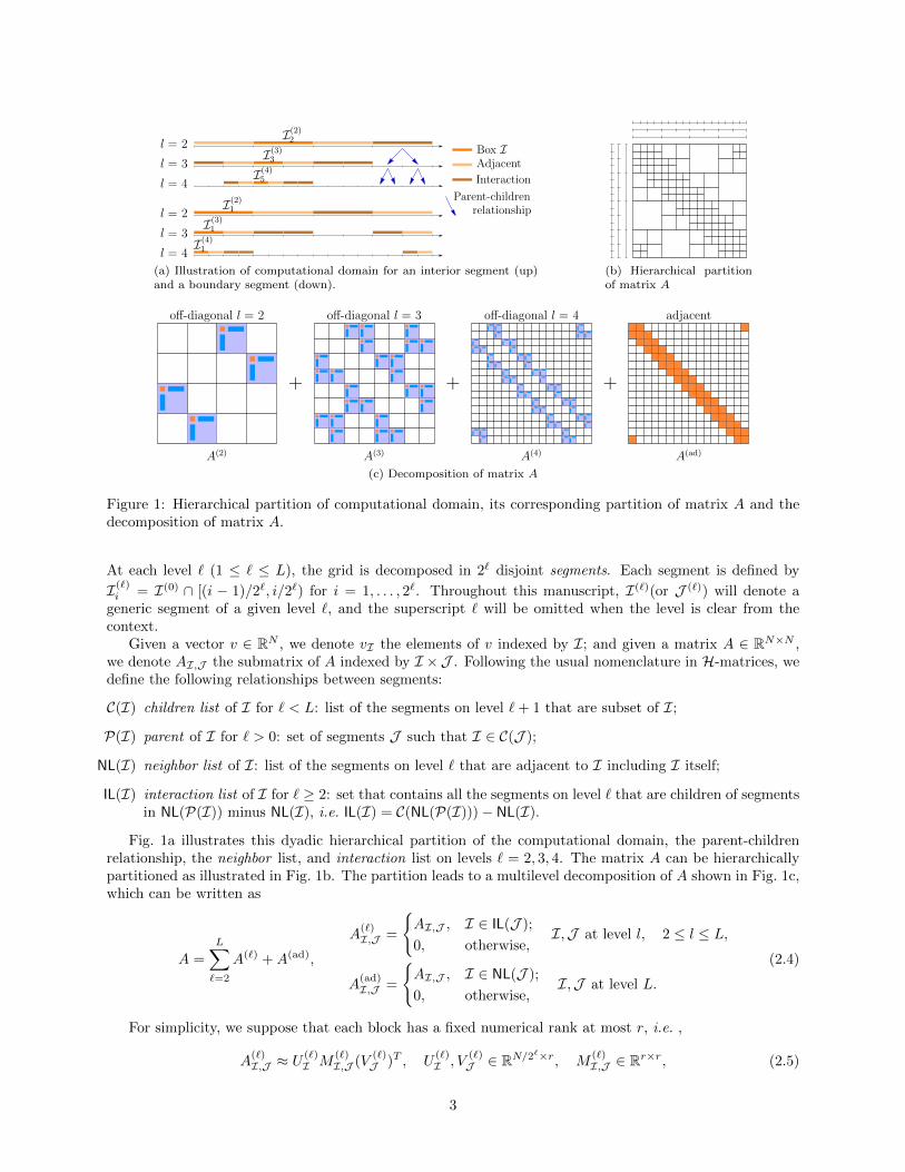
Figure 1: Hierarchical partition of computational domain, its corresponding partition of matrix A and thedecomposition of matrix A.

At each level ` (1 ≤ ` ≤ L), the grid is decomposed in 2` disjoint segments. Each segment is defined by

I(`)i = I(0) ∩ [(i − 1)/2`, i/2`) for i = 1, . . . , 2`. Throughout this manuscript, I(`)(or J (`)) will denote a

generic segment of a given level `, and the superscript ` will be omitted when the level is clear from thecontext.

Given a vector v ∈ RN , we denote vI the elements of v indexed by I; and given a matrix A ∈ RN×N ,we denote AI,J the submatrix of A indexed by I ×J . Following the usual nomenclature in H-matrices, wedefine the following relationships between segments:

C(I) children list of I for ` < L: list of the segments on level `+ 1 that are subset of I;

P(I) parent of I for ` > 0: set of segments J such that I ∈ C(J );

NL(I) neighbor list of I: list of the segments on level ` that are adjacent to I including I itself;

IL(I) interaction list of I for ` ≥ 2: set that contains all the segments on level ` that are children of segmentsin NL(P(I)) minus NL(I), i.e. IL(I) = C(NL(P(I)))− NL(I).

Fig. 1a illustrates this dyadic hierarchical partition of the computational domain, the parent-childrenrelationship, the neighbor list, and interaction list on levels ` = 2, 3, 4. The matrix A can be hierarchicallypartitioned as illustrated in Fig. 1b. The partition leads to a multilevel decomposition of A shown in Fig. 1c,which can be written as

A =

L∑`=2

A(`) +A(ad),

A(`)I,J =

AI,J , I ∈ IL(J );

0, otherwise,I,J at level l, 2 ≤ l ≤ L,

A(ad)I,J =

AI,J , I ∈ NL(J );

0, otherwise,I,J at level L.

(2.4)

For simplicity, we suppose that each block has a fixed numerical rank at most r, i.e. ,

A(`)I,J ≈ U

(`)I M

(`)I,J (V

(`)J )T , U

(`)I , V

(`)J ∈ RN/2

`×r, M(`)I,J ∈ Rr×r, (2.5)

3

U (`) M (`) (V (`))T

(a) Low-rank approximation of A(`) with ` = 3

≈

U (`) U (`+1) B(`)

(b) Nested bases of U(`) with ` = 3

U (L) B(L−1) M (L−1) (C(L−1))T (V (L))T

(c) Nested low-rank approximation of A(`) with ` = 3 and L = 4

Figure 2: Low rank factorization and nested low rank factorization of A(l).

where I and J are any interacting segments at level `. We can approximate A(`) as A(`) ≈ U (`)M (`)(V (`))T

as depicted in Fig. 2a. Here U (`), V (`) are block diagonal matrices with diagonal blocks U(`)I and V

(`)I for I

at level `, respectively, and M (`) aggregates all the blocks M(`)I,J for all interacting segments I,J at level `.

The key feature of H2-matrices is that the bases matrices U(`)I and V

(`)I between parent and children

segments enjoy a nested low rank approximation. More precisely, if I is at level 2 ≤ l < L and J1,J2 ∈ C(I)

are at level l + 1, then U(l)I and V

(l)I satisfy the following approximation:

U(`)I ≈

(U

(`+1)J1

U(`+1)J2

)B(`)J1

B(`)J2

, V(`)I ≈

(V

(`+1)J1

V(`+1)J2

)C(`)J1

C(`)J2

, (2.6)

where B(`)Ji , C

(`)Ji ∈ Rr×r, i = 1, 2. As depicted by Fig. 2b, if we introduce the matrix B(l) (C(l)) that

aggregates all the blocks B(`)Ji (C

(`)Ji ) for all the parent-children pairs (I, Ji), (2.6) can be compactly written

as U (l) ≈ U (l+1)B(l) and V (l) ≈ V (l+1)C(l). Thus, the decomposition (2.4) can be further factorized as

A =

L∑`=2

A(`) +A(ad) ≈L∑`=2

U (L)B(L−1) · · ·B(`)M (`)(C(`))T · · · (C(L−1))T (V (L))T +A(ad). (2.7)

The matrix-vector multiplication of A with an arbitrary vector v can be approximated by

Av ≈L∑`=2

U (L)B(L−1) · · ·B(`)M (`)(C(`))T · · · (C(L−1))T (V (L))T v +A(ad)v. (2.8)

Algorithm 1 provides the implementation of the matrix-vector multiplication of H2-matrices. The keyproperties of the matrices U (L), V (L), B(`), C(`), M (`) and A(ad) are summarized as follows:

Property 1. The matrices

1. U (L) and V (L) are block diagonal matrices with block size N/2L × r;

4

Algorithm 1 Application of H2-matrices on a vector v ∈ RN .

1: u(ad) = A(ad)v;2: ξ(L) = (V (L))T v;3: for ` from L− 1 to 2 by −1 do4: ξ(`) = (C(`))T ξ(`+1);5: end for6: for ` from 2 to L do7: ζ(`) = M (`)ξ(`);8: end for

9: χ = 0;10: for ` from 2 to L− 1 do11: χ = χ+ ζ(`);12: χ = B(`)χ;13: end for14: χ = χ+ ζ(L);15: χ = U (L)χ;16: u = χ+ u(ad);

2. B(`) and C(`), ` = 2, · · · , L− 1 are block diagonal matrices with block size 2r × r;

3. M (`), ` = 2, · · · , L are block cyclic band matrices with block size r × r and band size n(`)b , which is 2

for ` = 2 and 3 for ` > 2;

4. A(ad) is a block cyclic band matrix with block size m×m with band size n(ad)b = 1.

2.2 Matrix-vector multiplication as a neural network

We represent the matrix-vector multiplication (2.8) using the framework of neural networks. We first intro-duce our main tool — locally connected network — in Section 2.2.1 and then present the neural networkrepresentation of (2.8) in Section 2.2.2.

2.2.1 Locally connected network

In order to simplify the notation, let us present the 1D case as an example. In this setup, an NN layer canbe represented by a 2-tensor with size α × Nx, where α is called the channel dimension and Nx is usuallycalled the spatial dimension. A locally connected network is a type of mapping between two adjacent layers,where the output of each neuron depends only locally on the input. If a layer ξ with size α×Nx is connectedto a layer ζ with size α′ ×N ′x by a locally connected (LC) network, then

ζc′,i = φ

(i−1)s+w∑j=(i−1)s+1

α∑c=1

Wc′,c;i,jξc,j + bc′,i

, i = 1, . . . , N ′x, c′ = 1, . . . , α′, (2.9)

where φ is a pre-specified function, called activation, usually chosen to be e.g. a linear function, a rectified-linear unit (ReLU) function or a sigmoid function. The parameters w and s are called the kernel windowsize and stride, respectively. Fig. 3 presents a sample of the LC network. Furthermore, we call the layer ζlocally connected layer (LC layer) hereafter.

𝑁"

𝑁"#

𝑠

𝑤

(a) α = α′ = 1

𝛼

𝛼#

(b) α = 2, α′ = 3

Figure 3: Sample of LC network with Nx = 12, s = 2, w = 4 and N ′x = 5.

In (2.9) the LC network is represented using tensor notation; however, we can reshape ζ and ξ to a vectorby column major indexing and W to a matrix and write (2.9) into a matrix-vector form as

ζ = φ(Wξ + b). (2.10)

5

For later usage, we define Reshape[n1, n2] to be the map that reshapes a tensor with size n′1×n′2 to a 2-tensorof size n1 × n2 such that n1n2 = n′1n

′2 by column major indexing. Here, we implicitly regard a vector with

size n as a 2-tensor with size 1× n.

s = w = NxN ′x

, s = 1, N ′x = Nxs = 1, w = 1, N ′x = Nx

Space

Layer

(a) LCR[φ;Nx, α,N′x, α′] with

Nx = 16, α = 2, N ′x = 8 andα′ = 3

(b) LCK[φ;Nx, α, α′, w] with

Nx = 8, α = α′ = 3 and w = 3(c) LCI[φ;Nx, α, α

′] withNx = 8, α = 3 and α′ = 4

Figure 4: Three instances of locally connected networks used to represent the matrix-vector multiplication.The upper portions of each column depict the patterns of the matrices and the lower portions are theirrespective analogs using locally connect networks.

Each LC network has 6 parameters, Nx, α, N ′x, α′, w and s. We define three types of LC networksby specifying some of their parameters. The upper figures in Fig. 4 depict its corresponding formula inmatrix-vector form (2.10), and the lower figures show a diagram of the map.

LCR Restriction map: set s = w = NxN ′x

in LC. This map represents the multiplication of a block diagonal

matrix with block sizes α′×sα and a vector with size Nxα. We denote this map by LCR[φ;Nx, α,N′x, α′].

The application of LCR[linear; 16, 2, 8, 3] is depicted in Fig. 4a.

LCK Kernel map: set s = 1 and N ′x = Nx. This map represents the multiplication of a periodically bandedblock matrix (with block size α′×α and band size w−1

2 ) with a vector of size Nxα. To account for theperiodicity, we periodic pad the input layer ξc,j on the spatial dimension to the size (Nx +w− 1)× α.We denote this map by LCK[φ;Nx, α, α

′, w], which contains two steps: the periodic padding of ξc,j onthe spatial dimension, and the application of (2.9). The application of LCK[linear; 8, 3, 3, 3] is depictedin Fig. 4b.

LCI Interpolation map: set s = w = 1 and N ′x = Nx in LC. This map represents the multiplication ofa block diagonal matrix with block size α′ × α, times a vector of size Nxα. We denote the map byLCI[φ;Nx, α, α

′]. The application of LCI[linear; 8, 3, 4] is depicted in Fig. 4c.

2.2.2 Neural network representation

We need to find a neural network representation of the following 6 operations in order to perform thematrix-vector multiplication (2.8) for H2-matrices:

ξ(L) = (V (L))T v, (2.11a)

ξ(`) = (C(`))T ξ(`+1), 2 ≤ ` < L, (2.11b)

ζ(`) = M (`)ξ(`), 2 ≤ ` ≤ L, (2.11c)

6

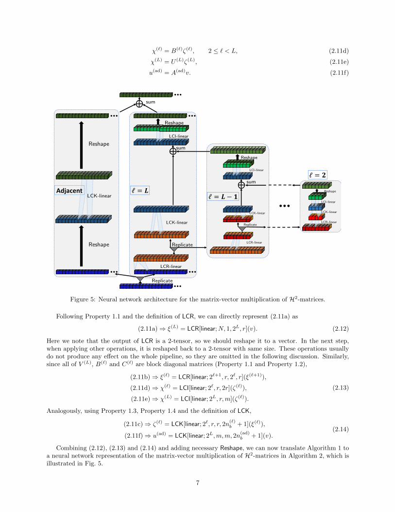
χ(`) = B(`)ζ(`), 2 ≤ ` < L, (2.11d)

χ(L) = U (L)ζ(L), (2.11e)

u(ad) = A(ad)v. (2.11f)

ℓ = #ℓ = # − %

Adjacent

ℓ = &

Reshape

Reshape

LCK-linear

Replicate

sum

Reshape

Replicate

sum

LCR-linear

LCK-linear

LCI-linear

Replicate

sum

Reshape

LCR-linear

LCK-linear

LCI-linear

LCR-linear

LCK-linear

LCI-linear

Reshape

Figure 5: Neural network architecture for the matrix-vector multiplication of H2-matrices.

Following Property 1.1 and the definition of LCR, we can directly represent (2.11a) as

(2.11a)⇒ ξ(L) = LCR[linear;N, 1, 2L, r](v). (2.12)

Here we note that the output of LCR is a 2-tensor, so we should reshape it to a vector. In the next step,when applying other operations, it is reshaped back to a 2-tensor with same size. These operations usuallydo not produce any effect on the whole pipeline, so they are omitted in the following discussion. Similarly,since all of V (L), B(`) and C(`) are block diagonal matrices (Property 1.1 and Property 1.2),

(2.11b)⇒ ξ(`) = LCR[linear; 2`+1, r, 2`, r](ξ(`+1)),

(2.11d)⇒ χ(`) = LCI[linear; 2`, r, 2r](ζ(`)),

(2.11e)⇒ χ(L) = LCI[linear; 2L, r,m](ζ(`)).

(2.13)

Analogously, using Property 1.3, Property 1.4 and the definition of LCK,

(2.11c)⇒ ζ(`) = LCK[linear; 2`, r, r, 2n(`)b + 1](ξ(`)),

(2.11f)⇒ u(ad) = LCK[linear; 2L,m,m, 2n(ad)b + 1](v).

(2.14)

Combining (2.12), (2.13) and (2.14) and adding necessary Reshape, we can now translate Algorithm 1 toa neural network representation of the matrix-vector multiplication of H2-matrices in Algorithm 2, which isillustrated in Fig. 5.

7

Algorithm 2 Application of NN architecture for H2-matrices on a vector v ∈ RN .

1: v = Reshape[m, 2L](v);

2: u(ad) = LCK[linear; 2L,m,m, 2n(ad)b + 1](v);

3: u(ad) = Reshape[1, N ](u(ad));4: ξ(L) = LCR[linear;N, 1, 2L, r](v);5: for ` from L− 1 to 2 by −1 do6: ξ(`) = LCR[linear; 2`+1, r, 2`, r](ξ(`+1));7: end for8: for ` from 2 to L do9: ζ(`) = LCK[linear; 2`, r, r, 2n

(`)b + 1](ξ(`));

10: end for

11: χ = 0;12: for ` from 2 to L− 1 do13: χ = χ+ ζ(`);14: χ = LCI[linear; 2`, r, 2r](χ);15: χ = Reshape[r, 2`+1](χ);16: end for17: χ = χ+ ζ(L);18: χ = LCI[linear; 2L, r,m](χ);19: χ = Reshape[1, N ](χ);20: u = χ+ u(ad);

Let us now calculate the number of parameters used in the network in Algorithm 2. For simplicity, weignore the number of parameters in the bias terms b and only consider the ones in the weight matrices W .Given that the number of parameters in an LC layer is N ′xαα

′w, the number of parameters for each type ofnetwork is:

NLCRp = Nxαα

′, NLCKp = Nxαα

′w, NLCIp = Nxαα

′, (2.15)

Then the total number of parameters in Algorithm 2 is

NH2

p = 2Lm2(2n(ad)b + 1) +Nr + 2

L−1∑`=2

2`+1r2 +

L∑`=2

2`r2(2n(`)b + 1) + 2Lrm

≤ Nm(2nb + 1) + 2Nr + 2Nr(2nb + 3)

≤ 3Nm(2nb + 3) = O(N),

(2.16)

where nb = max(n(ad)b , n

(`)b ), r ≤ m and 2Lm = N are used. The calculation shows that the number of

parameters in the neural network scales linearly in N and is therefore of the same order as the memorystorage in H2-matrices. This is lower than the quasilinear order O(N log(N)) of H-matrices and its neuralnetwork generalization.

2.3 Multi-dimensional case

Following the discussion in the previous section, Algorithm 2 can be easily extended to the d-dimensionalcase by performing a tensor-product of the one-dimensional case. In this subsection, we consider d = 2for instance, and the generalization to the d-dimensional case becomes straightforward. For the integralequation

u(x) =

∫Ω

g(x, y)v(y) dy, Ω = [0, 1)× [0, 1), (2.17)

we discretize it with an uniform grid with N × N , N = 2Lm, grid points and denote the resulting ma-trix obtained from the discretization of (2.17) by A. Conceptually Algorithm 2 required the following 3components:

1. multiscale decomposition of the matrix A, given by (2.4);

2. nested low-rank approximation of the far-field blocks of A, given by (2.6) and Property 1 for theresulting matrices;

3. definition of LC layers and theirs relationship (2.12),(2.13) and (2.14) with the matrices in Property 1.

We briefly explain how each step can be seamlessly extended to the higher dimension in what follows.

8

Multiscale decomposition. The grid is hierarchically partitioned into L+ 1 levels, in which each box is

defined by I(d,`)i = I(`)

i1⊗I(`)

i2, where i = (i1, i2) is a multi-dimensional index, I(`)

i1identifies the segments for

1D case and ⊗ is the tensor product. The definitions of the children list, parent, neighbor list and interactionlist can be easily extended. Each box I with ` < L has 4 children. Similarly, the decomposition (2.4) on Acan also be extended.

Nested low-rank approximation. Following the structure of H2-matrices, the nonzero blocks of A(`)

can be approximated by

A(`)I,J ≈ U

(`)I M

(`)I,J (V

(`)J )T , U

(`)I , V

(`)J ∈ R(N/2`)2×r, M

(`)I,J ∈ Rr×r, (2.18)

and the matrices U (`) satisfy the consistency condition, i.e.

U(`)I ≈

U

(`+1)J1

U(`+1)J2

U(`+1)J3

U(`+1)J4

B

(`)J1

B(`)J2

B(`)J3

B(`)J4

, (2.19)

where Jj are children of I, and B(`)Jj ∈ Rr×r, j = 1, . . . , 4. Similarly, the matrices V (`) also have the same

nested relationship.We denote an entry of a tensor T by Ti,j , where i is 2-dimensional index i = (i1, i2). Using the tensor

notations, U (L) and V (L) in (2.8) can be treated as 4-tensors of dimension N × N × 2Lr × 2L, while B(`)

and C(`) in (2.8) can be treated as 4-tensors of dimension 2`+1r× 2`+1 × 2`r× 2`. We generalize the notionof band matrix A to band tensors T by satisfying

Ti,j = 0, if |i1 − j1| > nb,1 or |i2 − j2| > nb,2, (2.20)

where nb = (nb,1, nb,2) is called the band size for tensor. Thus Property 1 can be extended to

Property 2. The 4-tensors

1. U (L) and V (L) are block diagonal tensors with block size N/2L ×N/2L × r × 1.

2. B(`) and C(`), ` = 2, · · · , L− 1 are block diagonal tensors with block size 2r × 2× r × 1

3. M (`), ` = 2, · · · , L are block cyclic band tensors with block size r× 1× r× 1 and band size n(`)b , which

is (2, 2) for ` = 2 and (3, 3) for ` > 2;

4. A(ad) is a block cyclic band matrix with block size m×m×m×m and band size n(ad)b = (1, 1).

LC layers. An NN layer for 2D can be represented by a 3-tensor of size α × Nx,1 × Nx,2, where α isthe channel dimension and Nx,1, Nx,2 are the spatial dimensions. If a layer ξ with size α × Nx,1 × Nx,2 isconnected to a locally connected layer ζ with size α′ ×N ′x,1 ×N ′x,2, then

ζc′,i = φ

(i−1)s+w∑j=(i−1)s+1

α∑c=1

Wc′,c;i,jξc,j + bc′,i

, i1 = 1, . . . , N ′x,1, i2 = 1, . . . , N ′x,2, c′ = 1, . . . , α′, (2.21)

where (i− 1)s = ((i1− 1)s1, (i2− 1)s2). As in the 1D case, the channel dimension corresponds to the rank r,and the spatial dimensions correspond to the grid points of the discretized domain. Analogously to the 1Dcase, we define the LC networks LCR, LCK and LCI and use them to express the 6 operations in (2.11) thatconstitute the building blocks of the neural network. The parameters Nx, s and w in the one-dimensional LCnetworks are replaced by their 2-dimensional counterpart Nx = (Nx,1, Nx,2), s = (s1, s2) and w = (w1, w2),

respectively. We point out that s = w = NxN ′x

for the 1D case is replaced by sj = wj =Nx,jN ′x,j

, j = 1, 2 for the

2D case in the definition of LC.

9

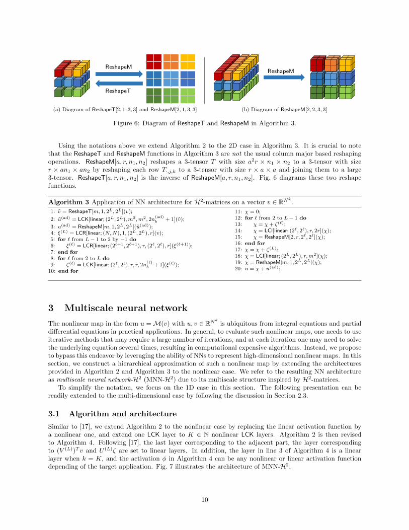
ReshapeT

ReshapeM

(a) Diagram of ReshapeT[2, 1, 3, 3] and ReshapeM[2, 1, 3, 3]

ReshapeM

(b) Diagram of ReshapeM[2, 2, 3, 3]

Figure 6: Diagram of ReshapeT and ReshapeM in Algorithm 3.

Using the notations above we extend Algorithm 2 to the 2D case in Algorithm 3. It is crucial to notethat the ReshapeT and ReshapeM functions in Algorithm 3 are not the usual column major based reshapingoperations. ReshapeM[a, r, n1, n2] reshapes a 3-tensor T with size a2r × n1 × n2 to a 3-tensor with sizer × an1 × an2 by reshaping each row T·,j,k to a 3-tensor with size r × a × a and joining them to a large3-tensor. ReshapeT[a, r, n1, n2] is the inverse of ReshapeM[a, r, n1, n2]. Fig. 6 diagrams these two reshapefunctions.

Algorithm 3 Application of NN architecture for H2-matrices on a vector v ∈ RN2

.

1: v = ReshapeT[m, 1, 2L, 2L](v);

2: u(ad) = LCK[linear; (2L, 2L),m2,m2, 2n(ad)b + 1](v);

3: u(ad) = ReshapeM[m, 1, 2L, 2L](u(ad));4: ξ(L) = LCR[linear; (N,N), 1, (2L, 2L), r](v);5: for ` from L− 1 to 2 by −1 do6: ξ(`) = LCR[linear; (2`+1, 2`+1), r, (2`, 2`), r](ξ(`+1));7: end for8: for ` from 2 to L do9: ζ(`) = LCK[linear; (2`, 2`), r, r, 2n

(`)b + 1](ξ(`));

10: end for

11: χ = 0;12: for ` from 2 to L− 1 do13: χ = χ+ ζ(`);14: χ = LCI[linear; (2`, 2`), r, 2r](χ);15: χ = ReshapeM[2, r, 2`, 2`](χ);16: end for17: χ = χ+ ζ(L);18: χ = LCI[linear; (2L, 2L), r,m2](χ);19: χ = ReshapeM[m, 1, 2L, 2L](χ);20: u = χ+ u(ad);

3 Multiscale neural network

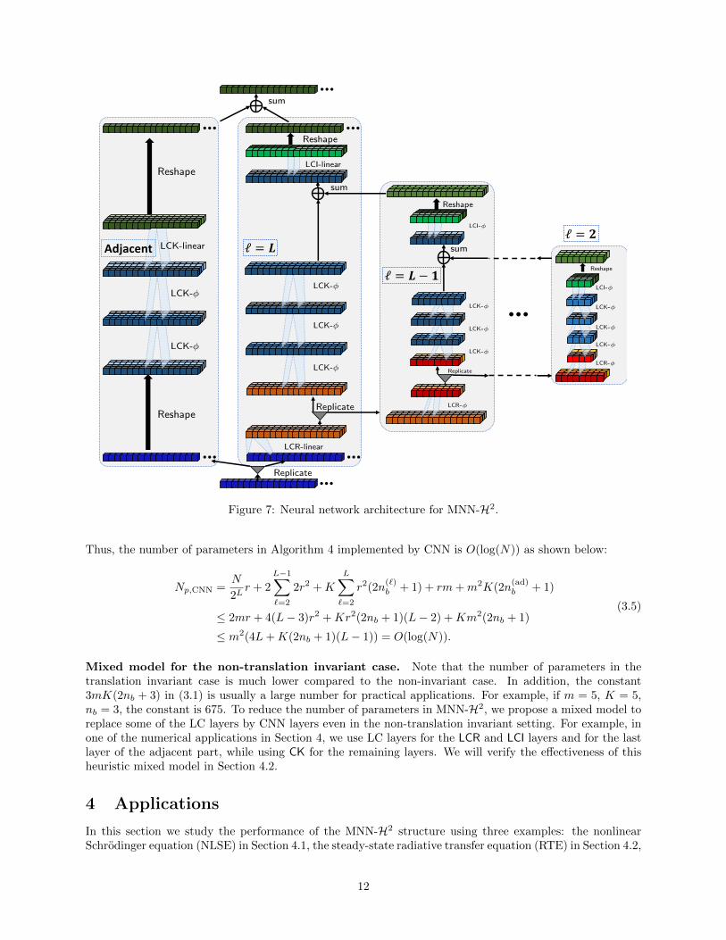
The nonlinear map in the form u =M(v) with u, v ∈ RNd is ubiquitous from integral equations and partialdifferential equations in practical applications. In general, to evaluate such nonlinear maps, one needs to useiterative methods that may require a large number of iterations, and at each iteration one may need to solvethe underlying equation several times, resulting in computational expensive algorithms. Instead, we proposeto bypass this endeavor by leveraging the ability of NNs to represent high-dimensional nonlinear maps. In thissection, we construct a hierarchical approximation of such a nonlinear map by extending the architecturesprovided in Algorithm 2 and Algorithm 3 to the nonlinear case. We refer to the resulting NN architectureas multiscale neural network-H2 (MNN-H2) due to its multiscale structure inspired by H2-matrices.

To simplify the notation, we focus on the 1D case in this section. The following presentation can bereadily extended to the multi-dimensional case by following the discussion in Section 2.3.

3.1 Algorithm and architecture

Similar to [17], we extend Algorithm 2 to the nonlinear case by replacing the linear activation function bya nonlinear one, and extend one LCK layer to K ∈ N nonlinear LCK layers. Algorithm 2 is then revisedto Algorithm 4. Following [17], the last layer corresponding to the adjacent part, the layer correspondingto (V (L))T v and U (L)ζ are set to linear layers. In addition, the layer in line 3 of Algorithm 4 is a linearlayer when k = K, and the activation φ in Algorithm 4 can be any nonlinear or linear activation functiondepending of the target application. Fig. 7 illustrates the architecture of MNN-H2.

10

Algorithm 4 Application of MNN-H2 to a vector v ∈ RN .

1: ξ0 = Reshape[m, 2L](v);2: for k from 1 to K do do3: ξk = LCK[φ; 2L,m,m, 2n

(ad)b + 1](ξk−1);

4: end for5: u(ad) = Reshape[1, N ](ξK);

6: ζ(L)0 = LCR[linear;N, 1, 2L, r](v);

7: for ` from L− 1 to 2 by −1 do8: ζ

(`)0 = LCR[φ; 2`+1, r, 2`, r](ζ

(`+1)0 );

9: end for10: for ` from 2 to L do11: for k from 1 to K do12: ζ

(`)k = LCK[φ; 2`, r, r, 2n

(`)b + 1](ζ

(`)k−1);

13: end for14: end for

15: χ = 0;16: for ` from 2 to L− 1 do17: χ = χ+ ζ

(`)K ;

18: χ = LCI[φ; 2`, r, 2r](χ);19: χ = Reshape[r, 2`+1](χ);20: end for21: χ = χ+ ζ

(L)K ;

22: χ = LCI[linear; 2L, r,m](χ);23: χ = Reshape[1, N ](χ);24: u = χ+ u(ad);

Similarly to the linear case, we compute the number of parameters of MNN-H2 to obtain

Np,LC = 2Lm2K(2n(ad)b + 1) +Nr + 2

L−1∑`=2

2`+1r2 +K

L∑`=2

2`r2(2n(`)b + 1) + 2Lrm

≤ 2Nr + 2Nr(2 +K(2nb + 1)) +NmK(2nb + 1)

≤ 3NmK(2nb + 3) ∼ O(N).

(3.1)

Here the number of parameters in b from (2.9) is also ignored. Compared to H-matrices, the main savingof the arithmetic complexity of H2-matrices is its nested structure of U (`) and V (`). Therefore, accordinglycompared to MNN-H in [17], the main saving on the number of parameters of MNN-H2 comes from thenested structure of LCR and LCI layers in Algorithm 4.

3.2 Translation invariant case

For the linear system (2.1), if the kernel is of convolution type, i.e. g(x, y) = g(x − y), then the matrix Ais a Toeplitz matrix. As a result, the matrices M (`), A(ad), U (L), V (L), B(`) and C(`) are all block cyclicmatrices. In the more general nonlinear case, the operator M is translation invariant (or more accuratelytranslation equivariant) if

TM(v) =M(T v) (3.2)

holds for any translation operator T . This indicates that the weights Wc′,c;i,j and bias bc,i in (2.9) can beindependent of index i. This is the case of a convolutional neural network (CNN):

ζc′,i = φ

(i−1)s+w∑j=(i−1)s+1

α∑c=1

Wc′,c;jξc,j + bc′

, i = 1, . . . , N ′x, c′ = 1, . . . , α′, (3.3)

Note that the difference between this and an LC network is that here W and b are independent of i. Inthis convolutional setting, we shall instead refer to the LC layers LCR, LCK, and LCI as CR, CK, and CI,respectively. By replacing the LC layers in Algorithm 4 with the corresponding CNN layers, we obtain theneural network architecture for the translation invariant kernel. It is easy to calculate that the number ofparameters of CR, CK and CI are

NCRp =

NxN ′x

α′, NCKp = αα′w, NCI

p = αα′. (3.4)

11

ℓ = #ℓ = $

ℓ = $ − &Adjacent

Reshape

Reshape

LCK-φ

LCK-φ

LCK-linear

Replicate

sum

Reshape

Replicate

sum

LCR-linear

LCK-φ

LCK-φ

LCK-φ

LCI-linear

Replicate

sum

Reshape

LCR-φ

LCK-φ

LCK-φ

LCK-φ

LCI-φ

LCR-φ

LCK-φ

LCK-φ

LCK-φ

LCI-φ

Reshape

Figure 7: Neural network architecture for MNN-H2.

Thus, the number of parameters in Algorithm 4 implemented by CNN is O(log(N)) as shown below:

Np,CNN =N

2Lr + 2

L−1∑`=2

2r2 +K

L∑`=2

r2(2n(`)b + 1) + rm+m2K(2n

(ad)b + 1)

≤ 2mr + 4(L− 3)r2 +Kr2(2nb + 1)(L− 2) +Km2(2nb + 1)

≤ m2(4L+K(2nb + 1)(L− 1)) = O(log(N)).

(3.5)

Mixed model for the non-translation invariant case. Note that the number of parameters in thetranslation invariant case is much lower compared to the non-invariant case. In addition, the constant3mK(2nb + 3) in (3.1) is usually a large number for practical applications. For example, if m = 5, K = 5,nb = 3, the constant is 675. To reduce the number of parameters in MNN-H2, we propose a mixed model toreplace some of the LC layers by CNN layers even in the non-translation invariant setting. For example, inone of the numerical applications in Section 4, we use LC layers for the LCR and LCI layers and for the lastlayer of the adjacent part, while using CK for the remaining layers. We will verify the effectiveness of thisheuristic mixed model in Section 4.2.

4 Applications

In this section we study the performance of the MNN-H2 structure using three examples: the nonlinearSchrodinger equation (NLSE) in Section 4.1, the steady-state radiative transfer equation (RTE) in Section 4.2,

12

and the Kohn-Sham map in Section 4.3.The MNN-H2 structure was implemented in Keras [13], a high-level neural network application program-

ming interface (API) running on top of TensorFlow [1], which is an open source software library for highperformance numerical computation. The loss function is chosen as the mean squared error. The opti-mization is performed using the Nadam optimizer [57]. The weights in MNN-H2 are initialized randomlyfrom the normal distribution and the batch size is always set between 1/100th and 1/50th of the number oftraining samples. As discussed in Section 3.2, if the operator M is translation invariant, all the layers areimplemented using CNN layers, otherwise we use LC layers or a mixture of LC and CNN layers.

In all the tests, the band size is chosen as nb,ad = 1 and n(`)b is 2 for ` = 2 and 3 otherwise. The activation

function in LCR and LCI is chosen to be linear, while ReLU is used in LCK. All the tests are run on GPUwith data type float32. The selection of parameters r (number of channels), L (N = 2Lm) and K (numberof layers in Algorithm 4) are problem dependent.

The training and test errors are measured by the relative error with respect to `2 norm

ε =||u− uNN ||`2||u||`2

. (4.1)

where u is the target solution generated by numerical discretization of PDEs and uNN is the predictionsolution by the neural network. We denote by εtrain and εtest the average training error and average testerror within a given set of samples, respectively. Similarly, we denote by σtrain and σtest the estimatedstandard deviation of the training and test errors within the given set of samples. The numerical resultspresented in this section are obtained by repeating the training a few times, using different random seeds.

4.1 NLSE with inhomogeneous background potential

The nonlinear Schrodinger equation (NLSE) is a widely used model in quantum physics to study phenomenonsuch as the Bose-Einstein condensation [2, 43]. It has been studied in [17] using the MNN-H structure. Inthis work, we use the same example to compare the results from MNN-H2 with those from MNN-H. Herewe study the NLSE with inhomogeneous background potential V (x)

−∆u(x) + V (x)u(x) + βu(x)3 = Eu(x), x ∈ [0, 1]d,

s.t.

∫[0,1]d

u(x)2 dx = 1, and

∫[0,1]d

u(x) dx > 0,(4.2)

with periodic boundary conditions, to find its ground state uG(x). We consider a defocusing cubic Schrodingerequation with a strong nonlinear term β = 10. The normalized gradient flow method in [5] is employed forthe numerical solution of NLSE.

In this work, we use neural networks to learn the map from the background potential to the ground state

V (x)→ uG(x). (4.3)

Clearly, this map is translation invariant, and thus MNN-H2 is implemented using CNN rather than LCnetwork. In the following, we study MNN-H2 on 1D and 2D cases, respectively.

In order to compare with MNN-H in [17], we choose the same potential V as in [17]

V (x) = −ng∑i=1

∞∑j1,...,jd=−∞

ρ(i)

√2πT

exp

(−|x− j − c

(i)|22T

), (4.4)

where the periodic summation imposes periodicity on the potential, and the parameters ρ(i) ∼ U(1, 4),c(i) ∼ U(0, 1)d, i = 1, . . . , ng and T ∼ U(2, 4)× 10−3.

4.1.1 One-dimensional case

For the one-dimensional case, we choose the number of discretization points N = 320, and set L = 7 andm = 5. The numerical experiments performed in this section use the same datasets as those in [17]. In that

13

0 0.5 1 1.5 2

104

0

0.5

1

1.5

2

2.5

310

-4

0

1

2

3

410

-4

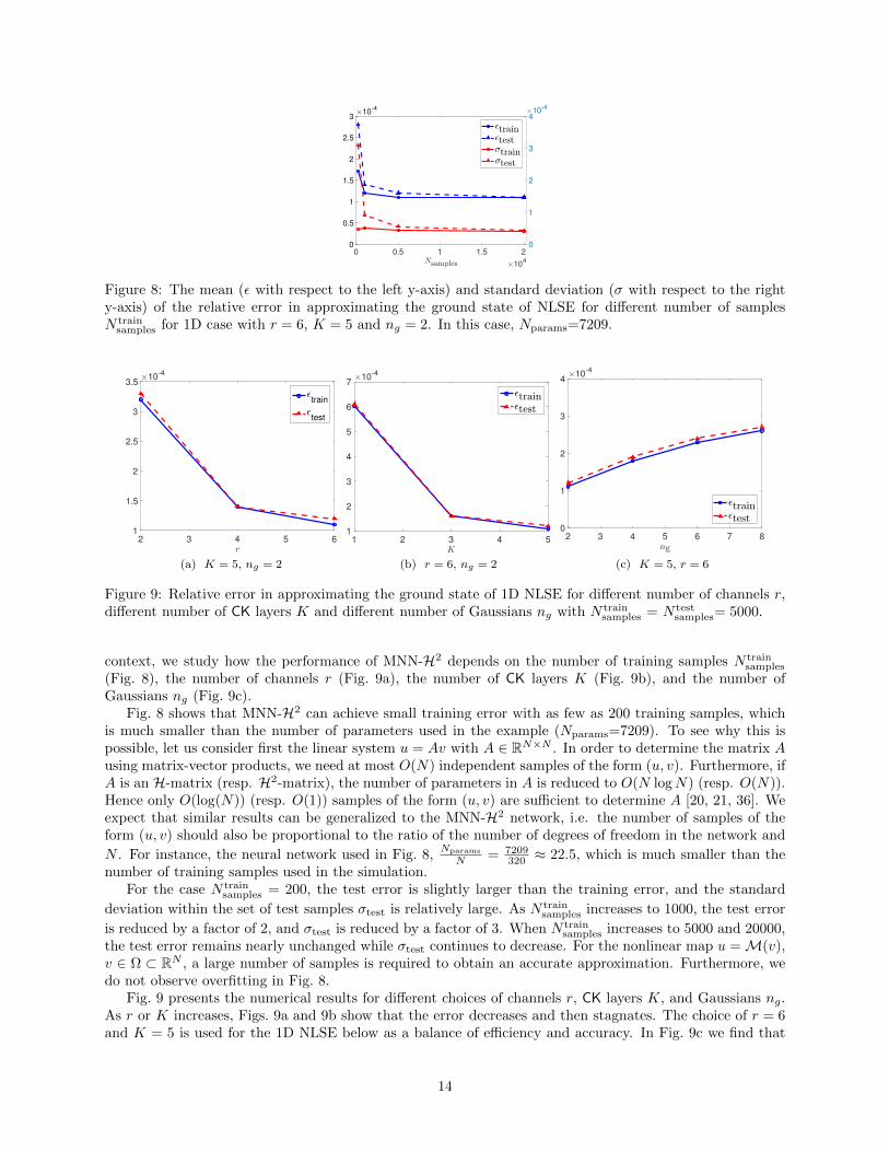
Figure 8: The mean (ε with respect to the left y-axis) and standard deviation (σ with respect to the righty-axis) of the relative error in approximating the ground state of NLSE for different number of samplesN train

samples for 1D case with r = 6, K = 5 and ng = 2. In this case, Nparams=7209.

2 3 4 5 61

1.5

2

2.5

3

3.510

-4

train

test

(a) K = 5, ng = 2

1 2 3 4 5

1

2

3

4

5

6

710

-4

(b) r = 6, ng = 2

2 3 4 5 6 7 8

0

1

2

3

410

-4

(c) K = 5, r = 6

Figure 9: Relative error in approximating the ground state of 1D NLSE for different number of channels r,different number of CK layers K and different number of Gaussians ng with N train

samples = N testsamples= 5000.

context, we study how the performance of MNN-H2 depends on the number of training samples N trainsamples

(Fig. 8), the number of channels r (Fig. 9a), the number of CK layers K (Fig. 9b), and the number ofGaussians ng (Fig. 9c).

Fig. 8 shows that MNN-H2 can achieve small training error with as few as 200 training samples, whichis much smaller than the number of parameters used in the example (Nparams=7209). To see why this ispossible, let us consider first the linear system u = Av with A ∈ RN×N . In order to determine the matrix Ausing matrix-vector products, we need at most O(N) independent samples of the form (u, v). Furthermore, ifA is an H-matrix (resp. H2-matrix), the number of parameters in A is reduced to O(N logN) (resp. O(N)).Hence only O(log(N)) (resp. O(1)) samples of the form (u, v) are sufficient to determine A [20, 21, 36]. Weexpect that similar results can be generalized to the MNN-H2 network, i.e. the number of samples of theform (u, v) should also be proportional to the ratio of the number of degrees of freedom in the network and

N . For instance, the neural network used in Fig. 8,Nparams

N = 7209320 ≈ 22.5, which is much smaller than the

number of training samples used in the simulation.For the case N train

samples = 200, the test error is slightly larger than the training error, and the standard

deviation within the set of test samples σtest is relatively large. As N trainsamples increases to 1000, the test error

is reduced by a factor of 2, and σtest is reduced by a factor of 3. When N trainsamples increases to 5000 and 20000,

the test error remains nearly unchanged while σtest continues to decrease. For the nonlinear map u =M(v),v ∈ Ω ⊂ RN , a large number of samples is required to obtain an accurate approximation. Furthermore, wedo not observe overfitting in Fig. 8.

Fig. 9 presents the numerical results for different choices of channels r, CK layers K, and Gaussians ng.As r or K increases, Figs. 9a and 9b show that the error decreases and then stagnates. The choice of r = 6and K = 5 is used for the 1D NLSE below as a balance of efficiency and accuracy. In Fig. 9c we find that

14

2 3 4 5 6

1

2

3

4

510

-4

(a) test error

2 3 4 5 6

0

2000

4000

6000

8000

10000

(b) Nparams

Figure 10: Numerical results of MNN-H / MNN-H2 for the minimum and median εtrain for 1D NLSE withrandom initial seed. The “min” and “median” stand for the test error corresponding to the minimum andmedian training data cases, respectively, and H and H2 stand for MNN-H and MNN-H2, respectively. Thesetup of MNN-H2 is K = 5, ng = 2, and N train

samples = N testsamples= 5000.

increasing the number of wells and hence the complexity of the input field, only leads to marginal increaseof the training and test errors.

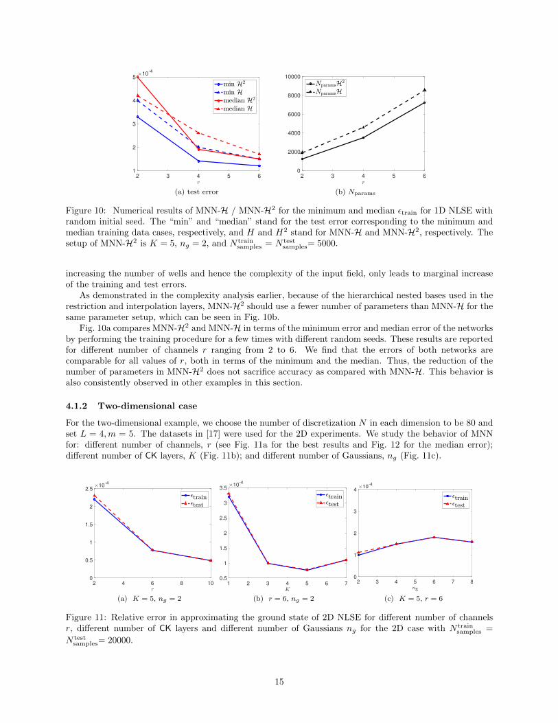
As demonstrated in the complexity analysis earlier, because of the hierarchical nested bases used in therestriction and interpolation layers, MNN-H2 should use a fewer number of parameters than MNN-H for thesame parameter setup, which can be seen in Fig. 10b.

Fig. 10a compares MNN-H2 and MNN-H in terms of the minimum error and median error of the networksby performing the training procedure for a few times with different random seeds. These results are reportedfor different number of channels r ranging from 2 to 6. We find that the errors of both networks arecomparable for all values of r, both in terms of the minimum and the median. Thus, the reduction of thenumber of parameters in MNN-H2 does not sacrifice accuracy as compared with MNN-H. This behavior isalso consistently observed in other examples in this section.

4.1.2 Two-dimensional case

For the two-dimensional example, we choose the number of discretization N in each dimension to be 80 andset L = 4,m = 5. The datasets in [17] were used for the 2D experiments. We study the behavior of MNNfor: different number of channels, r (see Fig. 11a for the best results and Fig. 12 for the median error);different number of CK layers, K (Fig. 11b); and different number of Gaussians, ng (Fig. 11c).

2 4 6 8 10

0

0.5

1

1.5

2

2.510

-4

(a) K = 5, ng = 2

1 2 3 4 5 6 7

0.5

1

1.5

2

2.5

3

3.510

-4

(b) r = 6, ng = 2

2 3 4 5 6 7 8

0

1

2

3

410

-4

(c) K = 5, r = 6

Figure 11: Relative error in approximating the ground state of 2D NLSE for different number of channelsr, different number of CK layers and different number of Gaussians ng for the 2D case with N train

samples =

N testsamples= 20000.

15

2 4 6 8 10

0

0.2

0.4

0.6

0.8

1

1.2

1.410

-3

(a) test error

2 4 6 8 10

2

4

6

8

10

1210

4

(b) Nparams

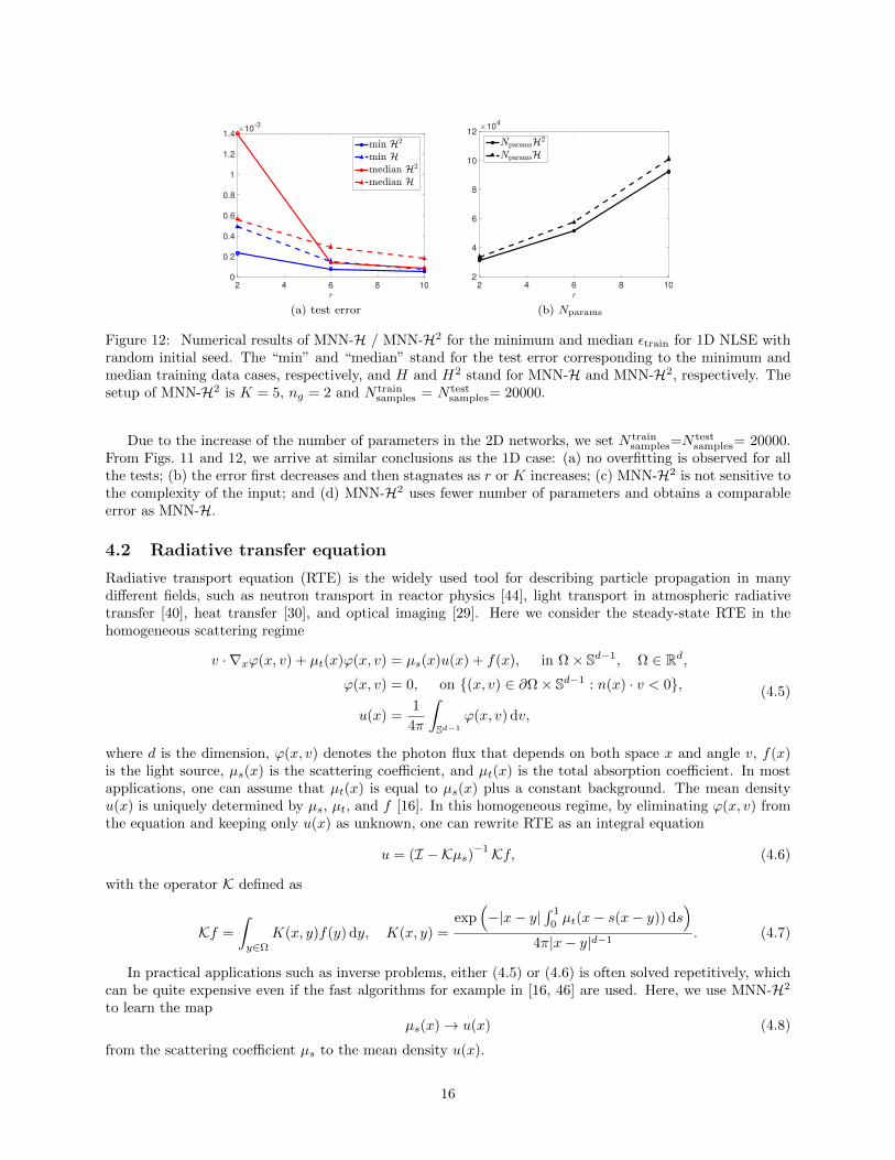
Figure 12: Numerical results of MNN-H / MNN-H2 for the minimum and median εtrain for 1D NLSE withrandom initial seed. The “min” and “median” stand for the test error corresponding to the minimum andmedian training data cases, respectively, and H and H2 stand for MNN-H and MNN-H2, respectively. Thesetup of MNN-H2 is K = 5, ng = 2 and N train

samples = N testsamples= 20000.

Due to the increase of the number of parameters in the 2D networks, we set N trainsamples=N

testsamples= 20000.

From Figs. 11 and 12, we arrive at similar conclusions as the 1D case: (a) no overfitting is observed for allthe tests; (b) the error first decreases and then stagnates as r or K increases; (c) MNN-H2 is not sensitive tothe complexity of the input; and (d) MNN-H2 uses fewer number of parameters and obtains a comparableerror as MNN-H.

4.2 Radiative transfer equation

Radiative transport equation (RTE) is the widely used tool for describing particle propagation in manydifferent fields, such as neutron transport in reactor physics [44], light transport in atmospheric radiativetransfer [40], heat transfer [30], and optical imaging [29]. Here we consider the steady-state RTE in thehomogeneous scattering regime

v · ∇xϕ(x, v) + µt(x)ϕ(x, v) = µs(x)u(x) + f(x), in Ω× Sd−1, Ω ∈ Rd,ϕ(x, v) = 0, on (x, v) ∈ ∂Ω× Sd−1 : n(x) · v < 0,

u(x) =1

4π

∫Sd−1

ϕ(x, v) dv,

(4.5)

where d is the dimension, ϕ(x, v) denotes the photon flux that depends on both space x and angle v, f(x)is the light source, µs(x) is the scattering coefficient, and µt(x) is the total absorption coefficient. In mostapplications, one can assume that µt(x) is equal to µs(x) plus a constant background. The mean densityu(x) is uniquely determined by µs, µt, and f [16]. In this homogeneous regime, by eliminating ϕ(x, v) fromthe equation and keeping only u(x) as unknown, one can rewrite RTE as an integral equation

u = (I − Kµs)−1Kf, (4.6)

with the operator K defined as

Kf =

∫y∈Ω

K(x, y)f(y) dy, K(x, y) =exp

(−|x− y|

∫ 1

0µt(x− s(x− y)) ds

)4π|x− y|d−1

. (4.7)

In practical applications such as inverse problems, either (4.5) or (4.6) is often solved repetitively, whichcan be quite expensive even if the fast algorithms for example in [16, 46] are used. Here, we use MNN-H2

to learn the mapµs(x)→ u(x) (4.8)

from the scattering coefficient µs to the mean density u(x).

16

4.2.1 One-dimensional slab geometry case

We first study the one-dimensional slab geometry case for d = 3, i.e. the parameters are homogeneous onthe direction x2 and x3. With slight abuse of notations, we denote x1 by x in this subsection. Then, (4.6)turns to

u(x) = (I − K1µs)−1K1f(x), (4.9)

where the operator K1 is defined as

K1f(x) =

∫y∈Ω

K1(x, y)f(x) dy,

K1(x, y) =1

2Ei

(−|x− y|

∫ 1

0

µt(x− s(x− y)) ds

),

(4.10)

and Ei(·) is the exponential integral.

2 4 6 8 100

0.5

1

1.510

-3

0

1

2

3

410

5

(a) K = 5, ng = 2

2 4 6

2

4

6

8

10

1210

-4

0.5

1

1.5

210

5

(b) ng = 2

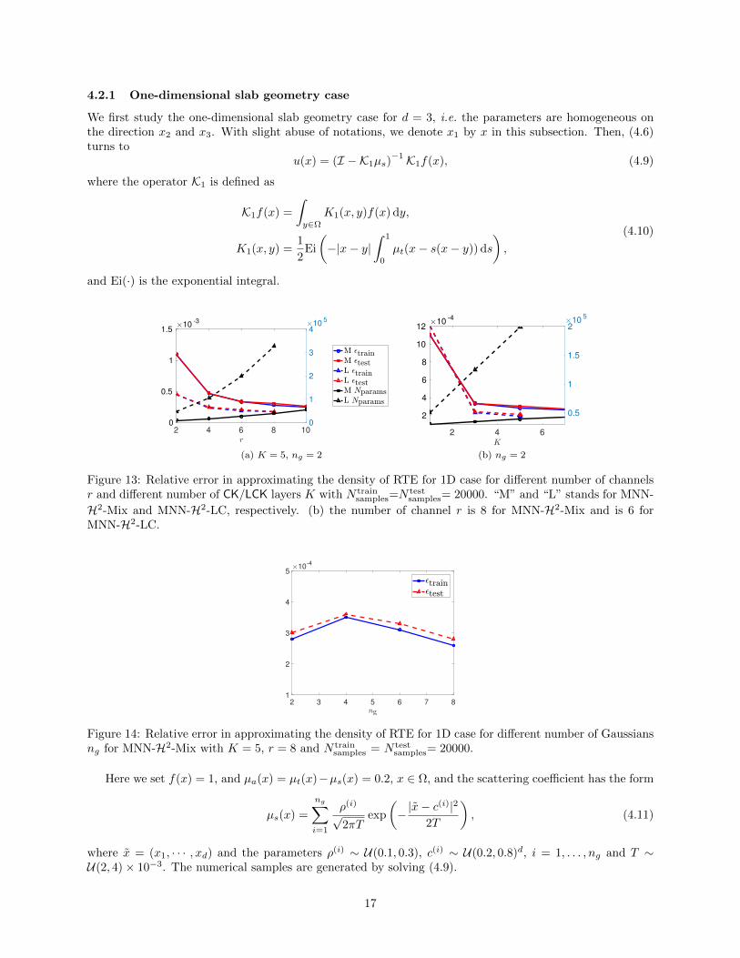
Figure 13: Relative error in approximating the density of RTE for 1D case for different number of channelsr and different number of CK/LCK layers K with N train

samples=Ntestsamples= 20000. “M” and “L” stands for MNN-

H2-Mix and MNN-H2-LC, respectively. (b) the number of channel r is 8 for MNN-H2-Mix and is 6 forMNN-H2-LC.

2 3 4 5 6 7 8

1

2

3

4

510

-4

Figure 14: Relative error in approximating the density of RTE for 1D case for different number of Gaussiansng for MNN-H2-Mix with K = 5, r = 8 and N train

samples = N testsamples= 20000.

Here we set f(x) = 1, and µa(x) = µt(x)−µs(x) = 0.2, x ∈ Ω, and the scattering coefficient has the form

µs(x) =

ng∑i=1

ρ(i)

√2πT

exp

(−|x− c

(i)|22T

), (4.11)

where x = (x1, · · · , xd) and the parameters ρ(i) ∼ U(0.1, 0.3), c(i) ∼ U(0.2, 0.8)d, i = 1, . . . , ng and T ∼U(2, 4)× 10−3. The numerical samples are generated by solving (4.9).

17

Because the map µs → u is translation invariant, MNN-H2 cannot be implemented using CNNs asbefore. As discussed at the end of Section 3.2, we can combine LC layers and CNN layers together to reducethe number of parameters. The resulting neural network is denoted by MNN-H2-Mix. As a reference, weimplement MNN-H2 by LC network and it is denoted by MNN-H2-LC. Note that since both µs and u arenot periodic the periodic padding in LCK/CK should be replaced by zero padding.

The number of discretization points is N = 320, and L = 6, m = 5. We perform numerical experimentsto study the numerical behavior for different number of channels (Fig. 13a) and different number of CK/LCKlayers K (Fig. 13b). For both MNN-H2-Mix and MNN-H2-LC, as r or K increase, the errors first decreaseand then stagnate. We use r = 8 and K = 5 for MNN-H2-Mix in the following. For the same setup,the error of MNN-H2-LC is somewhat smaller and the number of parameters is quite larger than that ofMNN-H2-Mix. Thus, MNN-H2-Mix serves as a good balance between the number of parameters and theaccuracy.

Fig. 14 summarizes the results of MNN-H2-Mix for different ng with K = 5 and r = 8. Numerical resultsshow that MNN-H2-Mix is not sensitive to the complexity of the input.

4.2.2 Two-dimensional case

Here we set f(x) = 1 and µa(x) = µt(x)− µs(x) = 0.2 for x ∈ Ω. The scattering coefficient takes the form

µs(x) =

2∑i=1

ρ(i)

√2πT

exp

(−|x− c

(i)|22T

), (4.12)

where x = (x1, x2) and the parameters ρ(i) ∼ U(0.01, 0.03), c(i) ∼ U(0.2, 0.8)2, i = 1, 2 and T ∼ U(2, 4) ×10−3. The numerical samples are generated by solving (4.6).

2 4 6 8 10 12 14

2

3

4

5

6

7

810

-4

Figure 15: Relative error in approximating the density of RTE for the 2D case for different number ofchannels for MNN-H2-Mix with K = 5 and N train

samples = N testsamples= 20000.

Because the map µs → u is not translation invariant, we implement the MNN-H2-Mix architecture asthe 1D case. Considering that the adjacent part takes a large number of parameters for the 2D case, weimplement the adjacent part by the CK layers. Fig. 15 gathers the results for different number of channelsr. Note that, similar to the 1D case, there is no overfitting for all the tests and the relative error decreasesas r increases.

4.3 Kohn-Sham map

In the Kohn-Sham density functional theory [25, 31], one needs to solve the following nonlinear eigenvalueequations (spin degeneracy omitted):(

−1

2∆ + V (x)

)ψi(x) = εiψi(x), x ∈ Ω = [−1, 1)d∫

Ω

ψi(x)ψj(x)dx = δij , ρ(x) =

ne∑i=1

|ψi(x)|2,(4.13)

18

where ne is the number of electrons, d is the spatial dimension, and δij stands for the Kronecker delta. Alleigenvalues εi are real and ordered non-decreasingly. The electron density ρ(x) satisfies the constraint

ρ(x) ≥ 0,

∫Ω

ρ(x) dx = ne. (4.14)

In this subsection, we employ the multiscale neural networks to approximate the Kohn-Sham map

FKS : V → ρ. (4.15)

The potential function V is given by

V (x) = −ne∑i=1

∑j∈Zd

ρ(i) exp

(− (x− c(i) − 2j)2

2σ2

), x ∈ [−1, 1)d, (4.16)

where c(i) ∈ [−1, 1)d and ρ(i) ∈ U(0.8, 1.2). We set σ = 0.05 for 1D and σ = 0.2 for the 2D case. The centersof the Gaussian wells c(i) are chosen randomly under the constraint that |c(i) − c(j)| > 2σ. The Kohn-Shammap is discretized using a pseudo-spectral method [58], and solved by a standard eigensolver.

4.3.1 One-dimensional case

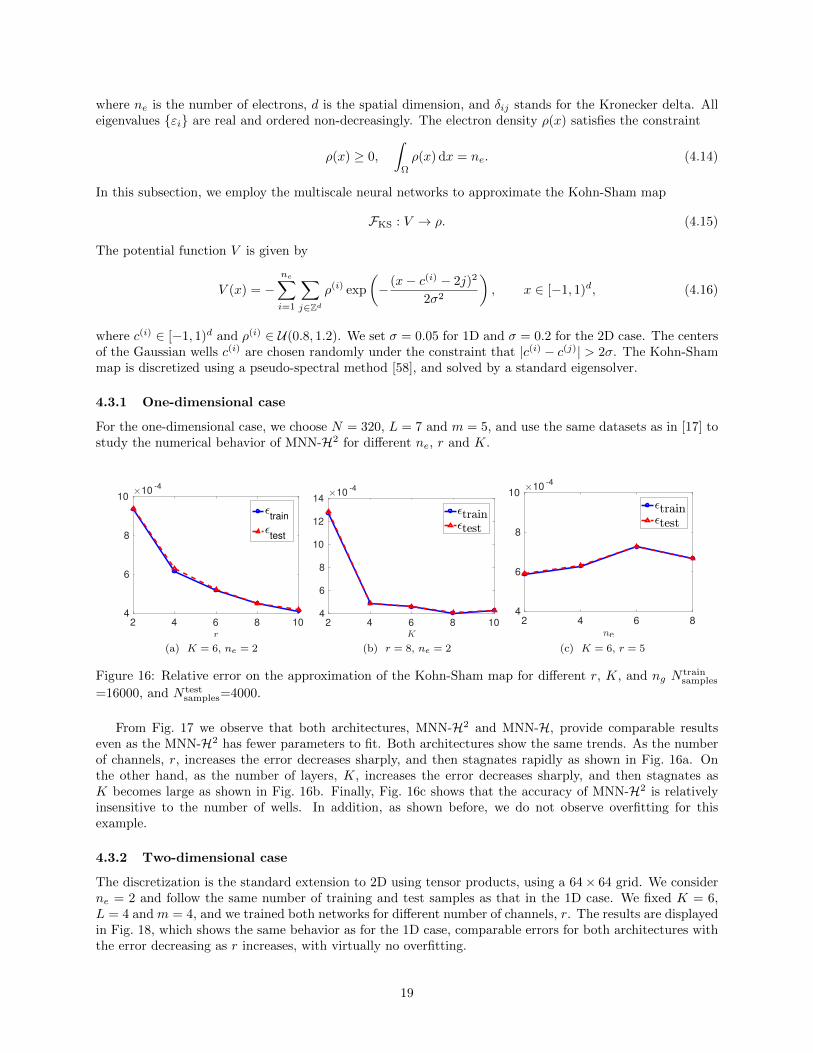
For the one-dimensional case, we choose N = 320, L = 7 and m = 5, and use the same datasets as in [17] tostudy the numerical behavior of MNN-H2 for different ne, r and K.

2 4 6 8 104

6

8

1010

-4

train

test

(a) K = 6, ne = 2

2 4 6 8 104

6

8

10

12

1410

-4

(b) r = 8, ne = 2

2 4 6 84

6

8

1010

-4

(c) K = 6, r = 5

Figure 16: Relative error on the approximation of the Kohn-Sham map for different r, K, and ng Ntrainsamples

=16000, and N testsamples=4000.

From Fig. 17 we observe that both architectures, MNN-H2 and MNN-H, provide comparable resultseven as the MNN-H2 has fewer parameters to fit. Both architectures show the same trends. As the numberof channels, r, increases the error decreases sharply, and then stagnates rapidly as shown in Fig. 16a. Onthe other hand, as the number of layers, K, increases the error decreases sharply, and then stagnates asK becomes large as shown in Fig. 16b. Finally, Fig. 16c shows that the accuracy of MNN-H2 is relativelyinsensitive to the number of wells. In addition, as shown before, we do not observe overfitting for thisexample.

4.3.2 Two-dimensional case

The discretization is the standard extension to 2D using tensor products, using a 64× 64 grid. We considerne = 2 and follow the same number of training and test samples as that in the 1D case. We fixed K = 6,L = 4 and m = 4, and we trained both networks for different number of channels, r. The results are displayedin Fig. 18, which shows the same behavior as for the 1D case, comparable errors for both architectures withthe error decreasing as r increases, with virtually no overfitting.

19

2 4 6 8 10

2

4

6

8

10

1210

-4

(a) test error

2 4 6 8 10

0

0.5

1

1.5

2

2.510

4

(b) Nparams

Figure 17: Numerical results of MNN-H / MNN-H2 for the minimum and median εtrain for 1D Kohn-Sham map with random initial seed. The “min” and “median” stand for the test error corresponding tothe minimum and median training data cases, respectively, and H and H2 stand for MNN-H and MNN-H2,respectively. The setup of MNN-H2 is K = 5, ng = 2 and N train

samples = N testsamples= 5000.

2 4 6 8 10

1

1.5

2

2.510

-3

Figure 18: Relative test error on the approximation of the 2D Kohn-Sham map for different number ofchannels r, and N train

samples = 16000.

5 Conclusion

In this paper, motivated by the fast multipole method (FMM) and H2-matrices, we developed a multiscaleneural network architecture (MNN-H2) to approximate nonlinear maps arising from integral equations andpartial differential equations. Using the framework of neural networks, MNN-H2 naturally generalizes H2-matrices to the nonlinear setting. Compared to the multiscale neural network based on hierarchical matrices(MNN-H), the distinguishing feature of MNN-H2 is that the interpolation and restriction layers are rep-resented using a set of nested layers, which reduces the computational and storage cost for large systems.Numerical results indicate that MNN-H2 can effectively approximate complex nonlinear maps arising fromthe nonlinear Schrodinger equation, the steady-state radiative transfer equation, and the Kohn-Sham densityfunctional theory. The MNN-H2 architecture can be naturally extended. For instance, the LCR and LCInetworks can involve nonlinear activation functions and can be extended to networks with more than onelayer. The LCK network can also be altered to other network structures, such as the sum of two parallelsubnetworks or the ResNet architecture [23].

Acknowledgements

The work of Y.F. and L.Y. is partially supported by the U.S. Department of Energy, Office of Science, Officeof Advanced Scientific Computing Research, Scientific Discovery through Advanced Computing (SciDAC)program and the National Science Foundation under award DMS-1818449. The work of J.F. is partiallysupported by “la Caixa” Fellowship, sponsored by the “la Caixa” Banking Foundation of Spain. The work

20

of L.L and L.Z. is partially supported by the Department of Energy under Grant No. DE-SC0017867 andthe CAMERA project.

References

[1] M. Abadi, P. Barham, J. Chen, Z. Chen, A. Davis, J. Dean, M. Devin, S. Ghemawat, G. Irving, M. Isard,et al. Tensorflow: A system for large-scale machine learning. In OSDI, volume 16, pages 265–283, 2016.

[2] J. R. Anglin and W. Ketterle. Bose–Einstein condensation of atomic gases. Nature, 416(6877):211,2002.

[3] M. Araya-Polo, J. Jennings, A. Adler, and T. Dahlke. Deep-learning tomography. The Leading Edge,37(1):58–66, 2018.

[4] V. Badrinarayanan, A. Kendall, and R. Cipolla. Segnet: A deep convolutional encoder-decoder ar-chitecture for image segmentation. IEEE Transactions on Pattern Analysis and Machine Intelligence,2017.

[5] W. Bao and Q. Du. Computing the ground state solution of Bose–Einstein condensates by a normalizedgradient flow. SIAM Journal on Scientific Computing, 25(5):1674–1697, 2004.

[6] C. Beck, W. E, and A. Jentzen. Machine learning approximation algorithms for high-dimensionalfully nonlinear partial differential equations and second-order backward stochastic differential equations.arXiv:1709.05963, 2017.

[7] J. Berg and K. Nystrom. A unified deep artificial neural network approach to partial differentialequations in complex geometries. arXiv preprint arXiv:1711.06464, 2017.

[8] S. Borm, L. Grasedyck, and W. Hackbusch. Introduction to hierarchical matrices with applications.Engineering analysis with boundary elements, 27(5):405–422, 2003.

[9] J. Bruna and S. Mallat. Invariant scattering convolution networks. IEEE Transactions on PatternAnalysis and Machine Intelligence, 35(8):1872–1886, 2013.

[10] S. Chan and A. H. Elsheikh. A machine learning approach for efficient uncertainty quantification usingmultiscale methods. Journal of Computational Physics, 354:493 – 511, 2018.

[11] P. Chaudhari, A. Oberman, S. Osher, S. Soatto, and G. Carlier. Partial differential equations for trainingdeep neural networks. In 2017 51st Asilomar Conference on Signals, Systems, and Computers, pages1627–1631, 2017.

[12] L. C. Chen, G. Papandreou, I. Kokkinos, K. Murphy, and A. L. Yuille. Deeplab: Semantic image seg-mentation with deep convolutional nets, atrous convolution, and fully connected crfs. IEEE Transactionson Pattern Analysis and Machine Intelligence, 40(4):834–848, 2018.

[13] F. Chollet et al. Keras. https://keras.io, 2015.

[14] N. Cohen, O. Sharir, and A. Shashua. On the expressive power of deep learning: A tensor analysis.arXiv preprint arXiv:1603.00988, 2018.

[15] W. E, J. Han, and A. Jentzen. Deep learning-based numerical methods for high-dimensional parabolicpartial differential equations and backward stochastic differential equations. Communications in Math-ematics and Statistics, 5(4):349–380, 2017.

[16] Y. Fan, J. An, and L. Ying. Fast algorithms for integral formulations of steady-state radiative transferequation. arXiv preprint arXiv:1802.03061, 2018.

[17] Y. Fan, L. Lin, L. Ying, and L. Zepeda-Nunez. A multiscale neural network based on hierarchicalmatrices. arXiv preprint arXiv:1807.01883, 2018.

21

[18] I. Goodfellow, Y. Bengio, and A. Courville. Deep Learning. MIT Press, 2016. http://www.

deeplearningbook.org.

[19] L. Greengard and V. Rokhlin. A fast algorithm for particle simulations. Journal of computationalphysics, 73(2):325–348, 1987.

[20] W. Hackbusch. A sparse matrix arithmetic based on H-matrices. part I: Introduction to H-matrices.Computing, 62(2):89–108, 1999.

[21] W. Hackbusch and B. N. Khoromskij. A sparse H-matrix arithmetic: general complexity estimates.Journal of Computational and Applied Mathematics, 125(1-2):479–501, 2000.

[22] W. Hackbusch, B. N. Khoromskij, and S. Sauter. On H2-matrices. lectures on applied mathematics.Springer, 2000.

[23] K. He, X. Zhang, S. Ren, and J. Sun. Deep residual learning for image recognition. In Proceedings ofthe IEEE conference on computer vision and pattern recognition, pages 770–778, 2016.

[24] G. Hinton, L. Deng, D. Yu, G. E. Dahl, A. r. Mohamed, N. Jaitly, A. Senior, V. Vanhoucke, P. Nguyen,T. N. Sainath, and B. Kingsbury. Deep neural networks for acoustic modeling in speech recognition:The shared views of four research groups. IEEE Signal Processing Magazine, 29(6):82–97, 2012.

[25] P. Hohenberg and W. Kohn. Inhomogeneous electron gas. Physical review, 136(3B):B864, 1964.

[26] K. Hornik. Approximation capabilities of multilayer feedforward networks. Neural Networks, 4(2):251–257, 1991.

[27] Y. Khoo, J. Lu, and L. Ying. Solving parametric PDE problems with artificial neural networks. arXivpreprint arXiv:1707.03351, 2017.

[28] V. Khrulkov, A. Novikov, and I. Oseledets. Expressive power of recurrent neural networks.arXiv:1711.00811, 2018.

[29] A. D. Klose, U. Netz, J. Beuthan, and A. H. Hielscher. Optical tomography using the time-independentequation of radiative transfer–part 1: forward model. Journal of Quantitative Spectroscopy and RadiativeTransfer, 72(5):691–713, 2002.

[30] R. Koch and R. Becker. Evaluation of quadrature schemes for the discrete ordinates method. Journalof Quantitative Spectroscopy and Radiative Transfer, 84(4):423–435, 2004.

[31] W. Kohn and L. J. Sham. Self-consistent equations including exchange and correlation effects. Physicalreview, 140(4A):A1133, 1965.

[32] A. Krizhevsky, I. Sutskever, and G. E. Hinton. Imagenet classification with deep convolutional neuralnetworks. In Proceedings of the 25th International Conference on Neural Information Processing Systems- Volume 1, NIPS’12, pages 1097–1105, USA, 2012. Curran Associates Inc.

[33] Y. LeCun, Y. Bengio, and G. Hinton. Deep learning. Nature, 521(436), 2015.

[34] M. K. K. Leung, H. Y. Xiong, L. J. Lee, and B. J. Frey. Deep learning of the tissue-regulated splicingcode. Bioinformatics, 30(12):i121–i129, 2014.

[35] Y. Li, X. Cheng, and J. Lu. Butterfly-Net: Optimal function representation based on convolutionalneural networks. arXiv preprint arXiv:1805.07451, 2018.

[36] L. Lin, J. Lu, and L. Ying. Fast construction of hierarchical matrix representation from matrix–vectormultiplication. Journal of Computational Physics, 230(10):4071–4087, 2011.

[37] G. Litjens, T. Kooi, B. E. Bejnordi, A. A. A. Setio, F. Ciompi, M. Ghafoorian, J. A. W. M. van derLaak, B. van Ginneken, and C. I. Sanchez. A survey on deep learning in medical image analysis. MedicalImage Analysis, 42:60–88, 2017.

22

[38] R. F. M. D. Zeiler. Visualizing and understanding convolutional networks. Computer Vision - ECCV201413 European Conference, pages 818–833, 2014.

[39] J. Ma, R. P. Sheridan, A. Liaw, G. E. Dahl, and V. Svetnik. Deep neural nets as a method for quantitativestructureactivity relationships. Journal of Chemical Information and Modeling, 55(2):263–274, 2015.

[40] A. Marshak and A. Davis. 3D radiative transfer in cloudy atmospheres. Springer Science & BusinessMedia, 2005.

[41] H. Mhaskar, Q. Liao, and T. Poggio. Learning functions: When is deep better than shallow. arXivpreprint arXiv:1603.00988, 2018.

[42] P. Paschalis, N. D. Giokaris, A. Karabarbounis, G. Loudos, D. Maintas, C. Papanicolas, V. Spanoudaki,C. Tsoumpas, and E. Stiliaris. Tomographic image reconstruction using artificial neural networks.Nuclear Instruments and Methods in Physics Research Section A: Accelerators, Spectrometers, Detectorsand Associated Equipment, 527(1):211 – 215, 2004. Proceedings of the 2nd International Conference onImaging Technologies in Biomedical Sciences.

[43] L. Pitaevskii. Vortex lines in an imperfect Bose gas. Sov. Phys. JETP, 13(2):451–454, 1961.

[44] G. C. Pomraning. The equations of radiation hydrodynamics. Courier Corporation, 1973.

[45] M. Raissi and G. E. Karniadakis. Hidden physics models: Machine learning of nonlinear partial differ-ential equations. Journal of Computational Physics, 357:125 – 141, 2018.

[46] K. Ren, R. Zhang, and Y. Zhong. A fast algorithm for radiative transport in isotropic media. arXivpreprint arXiv:1610.00835, 2016.

[47] O. Ronneberger, P. Fischer, and T. Brox. U-net: Convolutional networks for biomedical image segmen-tation. In N. Navab, J. Hornegger, W. M. Wells, and A. F. Frangi, editors, Medical Image Computing andComputer-Assisted Intervention – MICCAI 2015, pages 234–241, Cham, 2015. Springer InternationalPublishing.

[48] K. Rudd, G. D. Muro, and S. Ferrari. A constrained backpropagation approach for the adaptivesolution of partial differential equations. IEEE Transactions on Neural Networks and Learning Systems,25(3):571–584, 2014.

[49] R. Sarikaya, G. E. Hinton, and A. Deoras. Application of deep belief networks for natural languageunderstanding. IEEE/ACM Transactions on Audio, Speech and Language Processing, 22(4):778–784,2014.

[50] J. Schmidhuber. Deep learning in neural networks: An overview. Neural Networks, 61:85–117, 2015.

[51] D. Silver, A. Huang, C. J. Maddison, L. S. A. Guez, G. V. D. Driessche, J. Schrittwieser, I. Antonoglou,V. Panneershelvam, and e. a. M. Lanctot. Mastering the game of go with deep neural networks andtree search. Nature, 529(7587):484489, 2016.

[52] K. Simonyan and A. Zisserman. Very deep convolutional networks for large-sacle image recognition.Computing ResearchRepository (CoRR), abs/1409.1556, 2014.

[53] R. Socher, Y. Bengio, and C. D. Manning. Deep learning for nlp (without magic). The 50th AnnualMeeting of the Association for Computational Linguistics, Tutorial Abstracts, 5, 2012.

[54] K. Spiliopoulos and J. Sirignano. Dgm: A deep learning algorithm for solving partial differentialequations. arXiv preprint arXiv:1708.07469, 2018.

[55] I. Sutskever, O. Vinyals, and Q. V. Le. Sequence to sequence learning with neural networks. InZ. Ghahramani, M. Welling, C. Cortes, N. D. Lawrence, and K. Q. Weinberger, editors, Advances inNeural Information Processing Systems 27, pages 3104–3112. Curran Associates, Inc., 2014.

23

[56] C. Szegedy, W. Liu, Y. Jia, P. Sermanet, S. Reed, D. Anguelov, D. Erhan, V. Vanhoucke, and A. Ra-binovich. Going deeper with convolutions. Computing ResearchRepository (CoRR), abs/1409.4842,2014.

[57] D. Timothy. Incorporating nesterov momentum into adam. 2015.

[58] L. Trefethen. Spectral Methods in MATLAB. Society for Industrial and Applied Mathematics, 2000.

[59] E. Tyrtyshnikov. Mosaic-skeleton approximations. Calcolo, 33(1-2):47–57 (1998), 1996. Toeplitz matri-ces: structures, algorithms and applications (Cortona, 1996).

[60] D. Ulyanov, A. Vedaldi, and V. Lempitsky. Deep image prior. arXiv:1711.10925, 2018.

[61] T. Wang, D. J. Wu, A. Coates, and A. Y. Ng. End-to-end text recognition with convolutional neuralnetworks. Pattern Recognition (ICPR), 2012 21st International Conference on Pattern Recognition(ICPR2012), pages 3304–3308, 2012.

[62] Y. Wang, C. W. Siu, E. T. Chung, Y. Efendiev, and M. Wang. Deep multiscale model learning. arXivpreprint arXiv:1806.04830, 2018.

[63] H. Y. Xiong and et al. The human splicing code reveals new insights into the genetic determinants ofdisease. Science, 347(6218), 2015.

24