a multiple-scale power series method for solving nonlinear

Communications in Numerical Analysis 2016 No.1 (2016) 37-49

Available online at www.ispacs.com/cna

Volume 2016, Issue 1, Year 2016 Article ID cna-00252, 13 Pages

doi:10.5899/2016/cna-00252

Research Article

A multiple-scale power series method for solving nonlinearordinary differential equations

Chein-Shan Liu1,2∗ , Chung-Lun Kuo2, Wun-Sin Jhao1

(1) Department of Civil Engineering, National Taiwan University, Taipei 106-17, Taiwan

(2) Center for Numerical Simulation Software in Engineering and Sciences, College of Mechanics and Materials,

Hohai University, Nanjing, Jiangsu 210098, China

Copyright 2016 c⃝ Chein-Shan Liu, Chung-Lun Kuo and Wun-Sin Jhao. This is an open access article distributed under the Creative CommonsAttribution License, which permits unrestricted use, distribution, and reproduction in any medium, provided the original work is properly cited.

AbstractThe power series solution is a cheap and effective method to solve nonlinear problems, like the Duffing-van der Poloscillator, the Volterra population model and the nonlinear boundary value problems. A novel power series method byconsidering the multiple scales Rk in the power term (t/Rk)

k is developed, which are derived explicitly to reduce theill-conditioned behavior in the data interpolation. In the method a huge value times a tiny value is avoided, such thatwe can decrease the numerical instability and which is the main reason to cause the failure of the conventional powerseries method. The multiple scales derived from an integral can be used in the power series expansion, which providevery accurate numerical solutions of the problems considered in this paper.

Keywords and phrases:Duffing-van der Pol oscillator; Volterra population model; Power series method; Multiple scales; Recursionformula.

1 Introduction

The differential transform method [1] has been used to find the periodic solutions of strongly nonlinear oscillator.Qaisi [2] has used the power series approach to solve undamped and unforced Duffing equation, and Schovanec andWhite [3] used the Taylor series method. Chen [4] has used a target function method for the solution of the Duffingoscillator, while the Laplace decomposition methods were introduced by Yusufoglu [5] and Khuri [6]. Yue et al. [7]have applied the optimal scale polynomial interpolation technique to obtain the periodic solutions of the Duffing equa-tion, and Dai et al. [8] have used the multiple scale time domain collocation method for solving nonlinear dynamicalsystems.The power series method (PSM) is a classical one to solve ordinary differential equations (ODEs), which is closelyrelated to the Taylor series method, but does not need an elaborate differential process to derive the expansion coeffi-cients. However, the PSM is not used as a general purpose algorithm, because it is necessary to derive the algebraicequation of recursion formula case by case. In this paper, we solve nonlinear problems through an effective com-bination of the power series expansion method together with a sequence of multiple scales. Usually, the resultingnonlinear algebraic equations are severely ill-conditioned when higher order power terms are taken into account inthe series solution. So a major issue is how to reduce the ill-condition of the resulting nonlinear algebraic equations.

∗Corresponding author. Email address: [email protected]

37

Communications in Numerical Analysis 2016 No.1 (2016) 37-49http://www.ispacs.com/journals/cna/2016/cna-00252/ 38

According to this principle we can derive a formula to compute the multiple scales explicitly. On the other hand,the recursion formula can be used to generate the new coefficients from the older ones through a nonlinear equation,which provides a semi-analytic solution of nonlinear ODE.The organization of this paper is given as follows. In Section 2 we propose a new multiple-scale power series method(MSPSM) for the numerical solutions of some nonlinear problems. In Section 3 we apply the MSPSM to solve aDuffing-van der Pol equation, comparing to exact solution and displaying the high accuracy of the MSPSM. TheVolterra population model of a species within a closed system is solved by the MSPSM in Section 4, while two non-linear boundary value problems (BVPs) are solved in Section 5 by the MSPSM. Finally, the conclusions are drawn inSection 6.

2 A multiple-scale power series method

The PSM gives a solution x(t) of a nonlinear ODE in the form of a power series:

x(t) =∞

∑k=0

Aktk. (2.1)

It is easy to derive the formula and implement it to solve the ODE by inserting Eq. (2.1) into the desired ODE, andcompute the solution x(t) at any time t when Ak are computed from the derived recursion formula. However, in thenumerical solution we can only take finite power terms and compute the solution to a finite time:

x(t) =n

∑k=0

Aktk, t ≤ t f , (2.2)

which is limited by the capacity of computer, and t f is limited by the radius of convergence.Although the series solution in Eq. (2.2) is convergent for all t within a radius of convergence; however, the increaseof n might lead to a divergent solution when t > 1 due to the appearance of tk. In order to overcome this defect, Liuand Jhao [9] have proposed

x(t) =n

∑k=0

ak

(t

R0

)k

, t ≤ t f , (2.3)

where R0 is a given characteristic length. However, we can further modify the power series solution in Eq. (2.3) by

x(t) =n

∑k=0

ak

(t

Rk

)k

, t ≤ t f , (2.4)

where Rk is a sequence of multiple scales to be determined below, and R0 = 1.The polynomial interpolation of data is an ill-posed problem and it makes the data interpolation by using the higher-order polynomials not being easy to numerical implementation. In order to overcome that difficulty, Liu and Atluri[10] have introduced a characteristic length into the high-order polynomials expansion, which improves the numericalstability and accuracy in the data interpolation. Then, Liu [11] has further proposed a half-order multiple-scalepolynomial interpolation technique, which provides a highly accurate numerical result for data interpolation. Basedon these studies, we propose a multiple-scale power series expansion as a mathematical tool for the numerical solutionof nonlinear problem.Comparing Eqs. (2.2) and (2.4) we have

Ak =ak

Rkk, k = 1, . . . ,n. (2.5)

Our strategy is to find suitable scales of Rk, which depend on n and the collocated nodal points t j, such that ak is easilyand less ill-posedly to be solved than solving Ak, because Aktk is hard to be realized numerically when k is a largeinteger and t > 1 [9]. When ak is solved we can use Eq. (2.5) to find Ak.In order to obtain Rk, we impose the following n interpolated conditions to Eq. (2.4):

x(ti) = xi, ti = it f /n i = 1, . . . ,n. (2.6)

International Scientific Publications and Consulting Services


Thus, we obtain a linear equations system to determine a0 and ak, k = 1, . . . ,n:

1 t1R1

t21

R22

. . .(

t1Rn

)n

1 t2R1

t22

R22

. . .(

t2Rn

)n

......

......

...

1 tnR1

t2n

R22

. . .(

tnRn

)n

a0a1a2...

an

=

x1x2...

xn

. (2.7)

For the optimally scaled polynomial in Eq. (2.4) we can take

Rk =

(1n

n

∑j=1

t2kj

)1/(2k)

, k = 1, . . . ,n, (2.8)

in which t j = jt f /n is a uniform temporal node. Such that each column of the coefficient matrix in Eq. (2.7) has thesame Euclidean norm

√n. The coefficient matrix in Eq. (2.7) with the above Rk, k = 1, . . . ,n is an equilibrated matrix

[12, 13], which leads to a much better conditioning of Eq. (2.7) than the original Vandermonde coefficient matrix withRk = 1, k = 1, . . . ,n.When t and n are quite large the multiple scales Rk for larger k cannot be obtained from Eq. (2.8), because t2k

j isoverflow when k is near to n. So, replacing the summation in Eq. (2.8) by the integral we can derive

Rk =

(1n

∫ t f

0t2kdt

)1/(2k)

=t(2k+1)/(2k)

f

[n(2k+1)]1/(2k), k = 1, . . . ,n. (2.9)

The above two approaches of Rk in Eqs. (2.8) and (2.9) are, respectively, called the discrete and continuous MSPSM.For a long term computation, Liu and Jhao [9] have modified the power series solution (2.3) by

x(t) =n

∑k=0

ak

(t − tiR0

)k

, ti ≤ t ≤ ti + t f /N, (2.10)

where the total time interval is divided into N sub-intervals. By the same token we can modify Eq. (2.4) to

x(t) =n

∑k=0

ak

(t − tiRk

)k

, ti ≤ t ≤ ti + t f /N, (2.11)

where

Rk =(ti + t f /N)(2k+1)/(2k)

[n(2k+1)]1/(2k), k = 1, . . . ,n. (2.12)

At the first sub-interval t1 = 0, a0 = x0 and a1 = y0R1, where x0 and y0 are, respectively, the initial displacementand velocity of a second-order ODE; then in the subsequent time interval t ∈ [ti, ti + t f /N], a0 and a1 are obtained byinserting the values at the end time of the preceding interval into a0 = x(ti) and a1 = R1y(ti). These modifications arecrucial in the applications of the power series method to the solutions of nonlinear ODEs in a long time interval.

3 Duffing-van der Pol oscillator

We use the above novel power series expansion method to solve the following Duffing-van der Pol oscillator[14, 15]:

x(t)+ [γ +βx2(t)]x(t)+αx(t)+ x3(t) = 0, (3.13)

of which by inserting Eq. (2.4) we can derive the following recursion formula:

ak+2 =−Rk+2

k+2

(k+2)(k+1)

(Ck +

αak

Rkk+βSk +

γ(k+1)ak+1

Rk+1k+1

), k = 0,1, . . . , (3.14)



where

Bk =k

∑j=0

a j

R jj

ak− j

Rk− jk− j

, Ck =k

∑j=0

ak− j

Rk− jk− j

B j, Sk =k

∑j=0

(k− j+1)ak− j+1

Rk− j+1k− j+1

B j, k = 0,1, . . . . (3.15)

In the above, Bk represents the quadratic term x2, Ck the cubic term x3, and Sk the term of xx2.By starting from the initial conditions with x(0) = a0 and x(0) = a1/R1, we can use Eq. (3.14) to iteratively generatethe coefficients ak, k = 2, . . . ,n, and then the solution of x(t) is given by Eq. (2.4).For a special case of Eq. (3.13) with α = 3/β 2 and γ = 4/β , it is one of the first-kind Abel equation. Chandrasekar etal. [17] showed that Eq. (3.13) can be transformed as

w′′(z)− β 2

2w2(z)w′(z) = 0, (3.16)

wherez := e−2t/β , w :=−xet/β . (3.17)

Then a particular solution is available:

x(t) =−√

3

β√

t0e2t/β −1, (3.18)

where t0 > 1 is an arbitrary constant. If t0 is given, then the initial conditions are given by

x(0) =−√

3β√

t0 −1, x(0) =

√3t0

β 2(t0 −1)3/2 . (3.19)

Conversely, if x(0) is given then we have

t0 = 1+3

β 2x2(0), x(0) =

√3t0

β 2(t0 −1)3/2 . (3.20)

The differential transform method (DTM) has been applied by Mukherjee et al. [14] to solve the above problem withgiven values of x(0) = −0.28868 and β = 3. By Eq. (3.20) we can obtain t0 and x(0). We apply the multiple-scalepower series method (MSPSM) to solve this problem with n = 6 as follows:

xMSPSM = 0.28868+0.1202841368t −0.03508337872t2 +0.01099856740t3

−0.003843741333t4 +0.001394483198t5 −0.0005109682262t6, (3.21)xDTM = 0.28868+0.120281305t −0.080187536t2 −0.019916649t3

−0.02341443t4 −0.019687577t5 −0.010351679t6. (3.22)

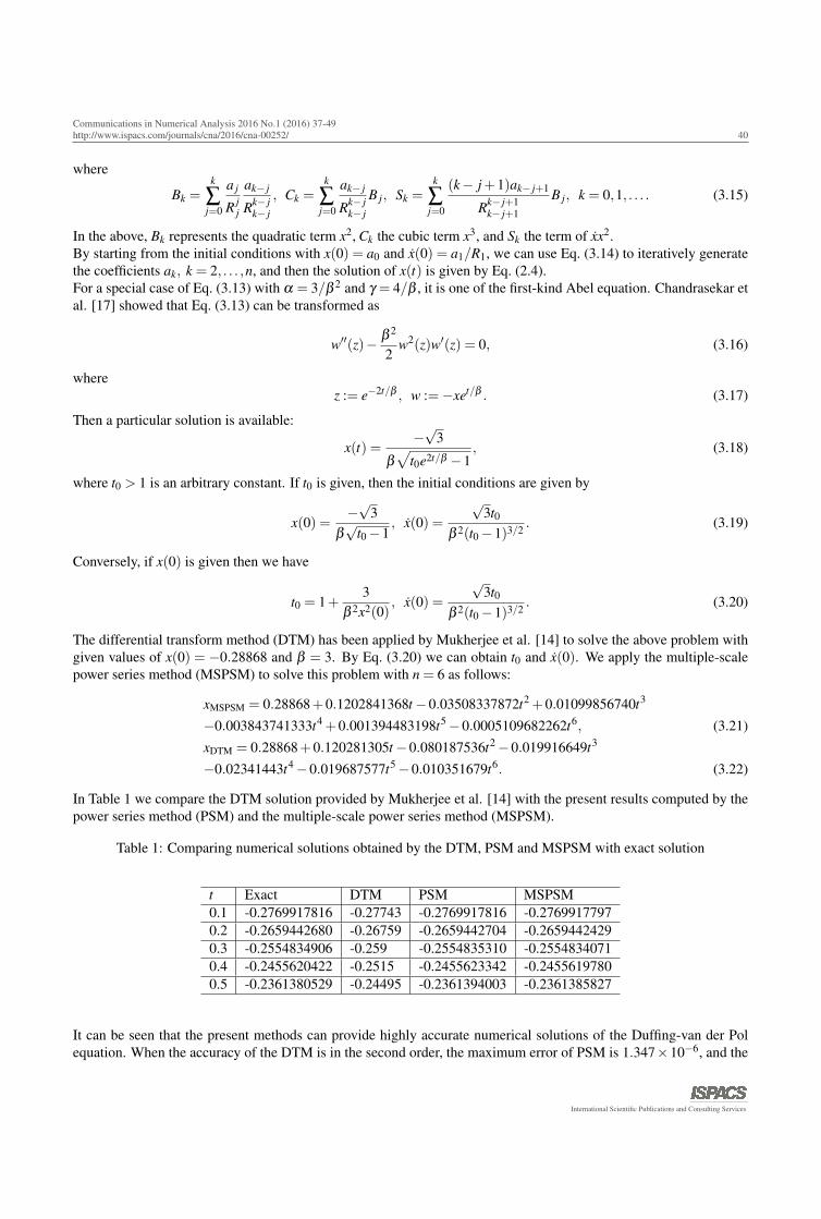
In Table 1 we compare the DTM solution provided by Mukherjee et al. [14] with the present results computed by thepower series method (PSM) and the multiple-scale power series method (MSPSM).

Table 1: Comparing numerical solutions obtained by the DTM, PSM and MSPSM with exact solution

t Exact DTM PSM MSPSM0.1 -0.2769917816 -0.27743 -0.2769917816 -0.27699177970.2 -0.2659442680 -0.26759 -0.2659442704 -0.26594424290.3 -0.2554834906 -0.259 -0.2554835310 -0.25548340710.4 -0.2455620422 -0.2515 -0.2455623342 -0.24556197800.5 -0.2361380529 -0.24495 -0.2361394003 -0.2361385827

It can be seen that the present methods can provide highly accurate numerical solutions of the Duffing-van der Polequation. When the accuracy of the DTM is in the second order, the maximum error of PSM is 1.347×10−6, and the



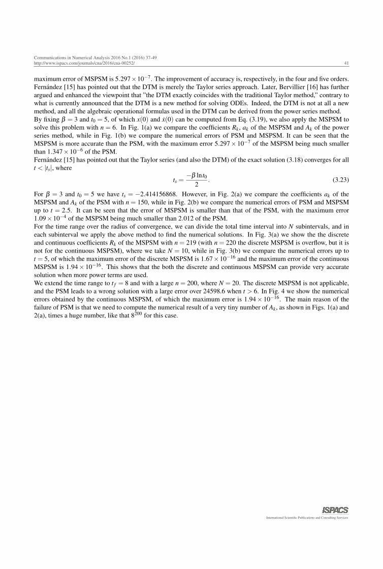
maximum error of MSPSM is 5.297×10−7. The improvement of accuracy is, respectively, in the four and five orders.Fernandez [15] has pointed out that the DTM is merely the Taylor series approach. Later, Bervillier [16] has furtherargued and enhanced the viewpoint that ”the DTM exactly coincides with the traditional Taylor method,” contrary towhat is currently announced that the DTM is a new method for solving ODEs. Indeed, the DTM is not at all a newmethod, and all the algebraic operational formulas used in the DTM can be derived from the power series method.By fixing β = 3 and t0 = 5, of which x(0) and x(0) can be computed from Eq. (3.19), we also apply the MSPSM tosolve this problem with n = 6. In Fig. 1(a) we compare the coefficients Rk, ak of the MSPSM and Ak of the powerseries method, while in Fig. 1(b) we compare the numerical errors of PSM and MSPSM. It can be seen that theMSPSM is more accurate than the PSM, with the maximum error 5.297× 10−7 of the MSPSM being much smallerthan 1.347×10−6 of the PSM.Fernandez [15] has pointed out that the Taylor series (and also the DTM) of the exact solution (3.18) converges for allt < |ts|, where

ts =−β ln t0

2. (3.23)

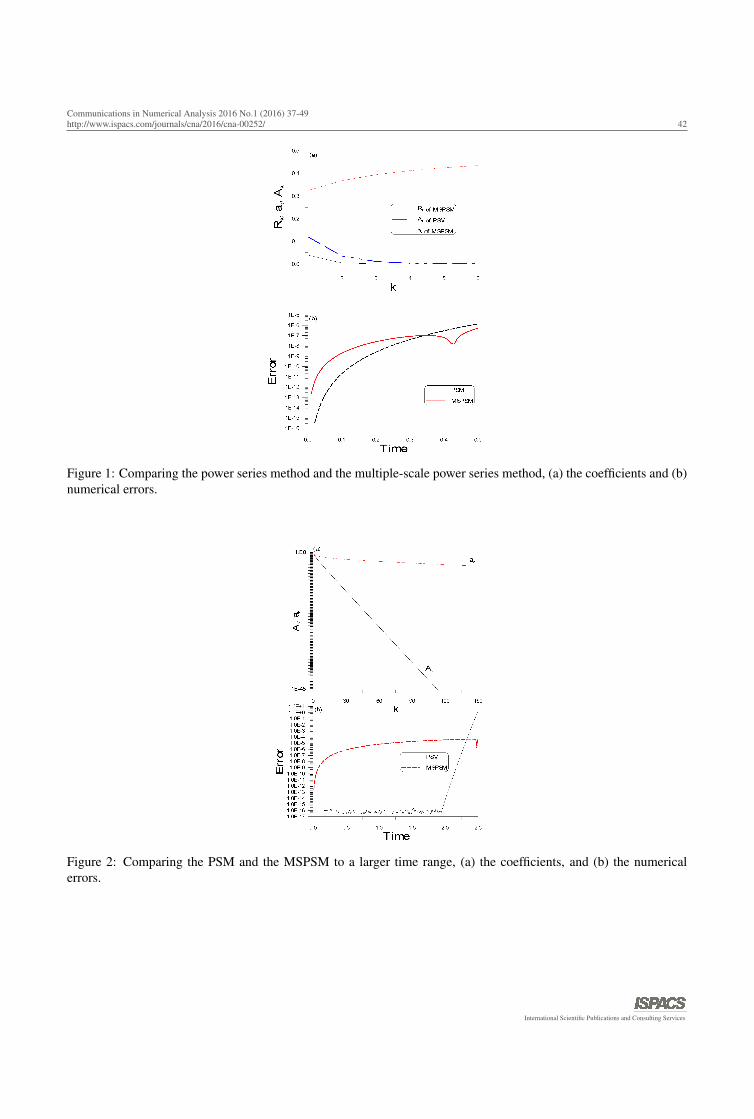
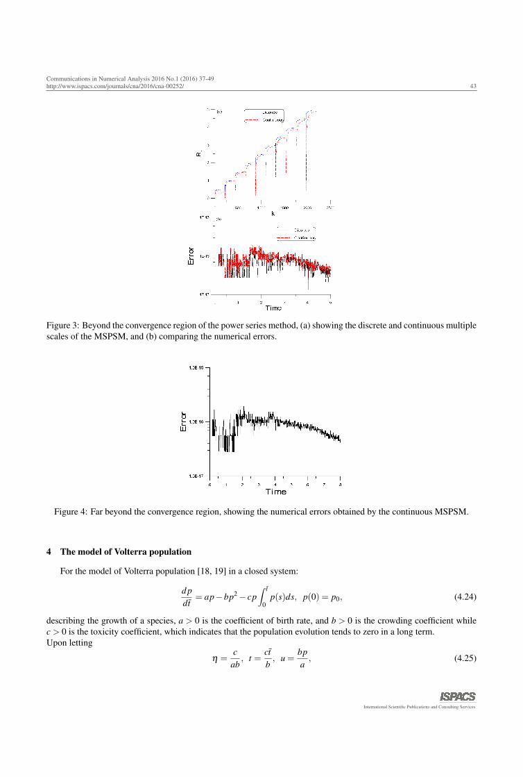
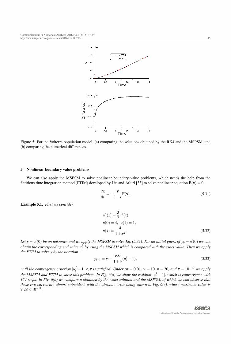
For β = 3 and t0 = 5 we have ts = −2.414156868. However, in Fig. 2(a) we compare the coefficients ak of theMSPSM and Ak of the PSM with n = 150, while in Fig. 2(b) we compare the numerical errors of PSM and MSPSMup to t = 2.5. It can be seen that the error of MSPSM is smaller than that of the PSM, with the maximum error1.09×10−4 of the MSPSM being much smaller than 2.012 of the PSM.For the time range over the radius of convergence, we can divide the total time interval into N subintervals, and ineach subinterval we apply the above method to find the numerical solutions. In Fig. 3(a) we show the the discreteand continuous coefficients Rk of the MSPSM with n = 219 (with n = 220 the discrete MSPSM is overflow, but it isnot for the continuous MSPSM), where we take N = 10, while in Fig. 3(b) we compare the numerical errors up tot = 5, of which the maximum error of the discrete MSPSM is 1.67×10−16 and the maximum error of the continuousMSPSM is 1.94× 10−16. This shows that the both the discrete and continuous MSPSM can provide very accuratesolution when more power terms are used.We extend the time range to t f = 8 and with a large n = 200, where N = 20. The discrete MSPSM is not applicable,and the PSM leads to a wrong solution with a large error over 24598.6 when t > 6. In Fig. 4 we show the numericalerrors obtained by the continuous MSPSM, of which the maximum error is 1.94× 10−16. The main reason of thefailure of PSM is that we need to compute the numerical result of a very tiny number of Ak, as shown in Figs. 1(a) and2(a), times a huge number, like that 8200 for this case.



Figure 1: Comparing the power series method and the multiple-scale power series method, (a) the coefficients and (b)numerical errors.

Figure 2: Comparing the PSM and the MSPSM to a larger time range, (a) the coefficients, and (b) the numericalerrors.



Figure 3: Beyond the convergence region of the power series method, (a) showing the discrete and continuous multiplescales of the MSPSM, and (b) comparing the numerical errors.

Figure 4: Far beyond the convergence region, showing the numerical errors obtained by the continuous MSPSM.

4 The model of Volterra population

For the model of Volterra population [18, 19] in a closed system:

d pdt

= ap−bp2 − cp∫ t

0p(s)ds, p(0) = p0, (4.24)

describing the growth of a species, a > 0 is the coefficient of birth rate, and b > 0 is the crowding coefficient whilec > 0 is the toxicity coefficient, which indicates that the population evolution tends to zero in a long term.Upon letting

η =c

ab, t =

ctb, u =

bpa, (4.25)



Eq. (4.24) is non-dimensionalized to a nonlinear Volterra differential-integral equation:

ηdudt

= u−u2 −u∫ t

0u(s)ds, u(0) = u0. (4.26)

There are many approximate and numerical solutions for Volterra’s population model, we name a few [18, 20, 21, 22,23, 24, 25, 26, 27, 28, 29, 30, 31, 32]. We can solve Eq. (4.26) by applying the MSPSM with the following recursionformula:

ak+1 =Rk+1

k+1

η(k+1)

(ak

Rkk−Bk −Dk

), k = 0,1, . . . , (4.27)

where

Bk =k

∑j=0

a j

R jj

ak− j

Rk− jk− j

, Ck =ak−1

kRk−1k−1

, Dk =k

∑j=0

a j

R jj

Ck− j, k = 1,2, . . . , (4.28)

in which Bk represents the quadratic term u2, Ck the integral term∫ t

0 u(s)ds, and Dk the product term u∫ t

0 u(s)ds. Forthe purpose of comparison we let

v(t) =∫ t

0u(s)ds, (4.29)

and then we have a system of two first-order ODEs:

u(t) =1η[u(t)−u2(t)−u(t)v(t)], u(0) = u0,

v(t) = u(t), v(0) = 0. (4.30)

We apply the fourth-order Runge-Kutta method (RK4) to integrate the above ODEs with a time increment ∆t. Underthe values of n = 300, η = 0.5, u0 = 0.1 and ∆t = 0.001, in Fig. 5(a) we compare u obtained by the RK4 and MSPSMto t = 1, of which we can observe that these two curves are almost coincident, with the absolute difference beingshown in Fig. 5(b), whose maximum value of difference is 8.66×10−15.



Figure 5: For the Volterra population model, (a) comparing the solutions obtained by the RK4 and the MSPSM, and(b) comparing the numerical differences.

5 Nonlinear boundary value problems

We can also apply the MSPSM to solve nonlinear boundary value problems, which needs the help from thefictitious time integration method (FTIM) developed by Liu and Atluri [33] to solve nonlinear equation F(x) = 0:

dxdt

=− ν1+ t

F(x). (5.31)

Example 5.1. First we consider

u′′(x) =32

u2(x),

u(0) = 4, u(1) = 1,

u(x) =4

1+ x2 . (5.32)

Let y = u′(0) be an unknown and we apply the MSPSM to solve Eq. (5.32). For an initial guess of y0 = u′(0) we canobtain the corresponding end value u f

i by using the MSPSM which is compared with the exact value. Then we applythe FTIM to solve y by the iteration:

yi+1 = yi −ν∆t

1+ ti(u f

i −1), (5.33)

until the convergence criterion |u fi − 1| < ε is satisfied. Under ∆t = 0.01, ν = 10, n = 20, and ε = 10−10 we apply

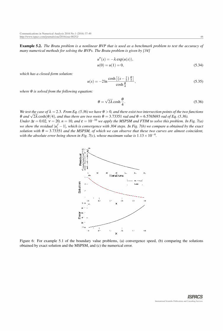
the MSPSM and FTIM to solve this problem. In Fig. 6(a) we show the residual |u fi − 1|, which is convergence with

154 steps. In Fig. 6(b) we compare u obtained by the exact solution and the MSPSM, of which we can observe thatthese two curves are almost coincident, with the absolute error being shown in Fig. 6(c), whose maximum value is9.28×10−11.



Example 5.2. The Bratu problem is a nonlinear BVP that is used as a benchmark problem to test the accuracy ofmany numerical methods for solving the BVPs. The Bratu problem is given by [34]

u′′(x) =−λ exp(u(x)),u(0) = u(1) = 0, (5.34)

which has a closed-form solution:

u(x) =−2lncosh

[(x− 1

2

) θ2

]cosh θ

4

, (5.35)

where θ is solved from the following equation:

θ =√

2λ coshθ4. (5.36)

We test the case of λ = 2.3. From Eq. (5.36) we have θ > 0, and there exist two intersection points of the two functionsθ and

√2λ cosh(θ/4), and thus there are two roots θ = 3.73351 rad and θ = 6.5765693 rad of Eq. (5.36).

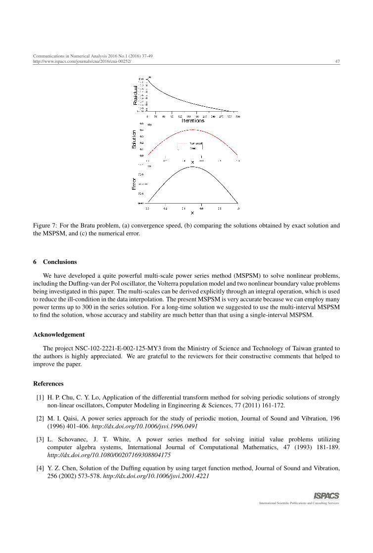
Under ∆t = 0.02, ν = 20, n = 10, and ε = 10−10 we apply the MSPSM and FTIM to solve this problem. In Fig. 7(a)we show the residual |u f

i −1|, which is convergence with 304 steps. In Fig. 7(b) we compare u obtained by the exactsolution with θ = 3.73351 and the MSPSM, of which we can observe that these two curves are almost coincident,with the absolute error being shown in Fig. 7(c), whose maximum value is 1.13×10−4.

Figure 6: For example 5.1 of the boundary value problems, (a) convergence speed, (b) comparing the solutionsobtained by exact solution and the MSPSM, and (c) the numerical error.



Figure 7: For the Bratu problem, (a) convergence speed, (b) comparing the solutions obtained by exact solution andthe MSPSM, and (c) the numerical error.

6 Conclusions

We have developed a quite powerful multi-scale power series method (MSPSM) to solve nonlinear problems,including the Duffing-van der Pol oscillator, the Volterra population model and two nonlinear boundary value problemsbeing investigated in this paper. The multi-scales can be derived explicitly through an integral operation, which is usedto reduce the ill-condition in the data interpolation. The present MSPSM is very accurate because we can employ manypower terms up to 300 in the series solution. For a long-time solution we suggested to use the multi-interval MSPSMto find the solution, whose accuracy and stability are much better than that using a single-interval MSPSM.

Acknowledgement

The project NSC-102-2221-E-002-125-MY3 from the Ministry of Science and Technology of Taiwan granted tothe authors is highly appreciated. We are grateful to the reviewers for their constructive comments that helped toimprove the paper.

References

[1] H. P. Chu, C. Y. Lo, Application of the differential transform method for solving periodic solutions of stronglynon-linear oscillators, Computer Modeling in Engineering & Sciences, 77 (2011) 161-172.

[2] M. I. Qaisi, A power series approach for the study of periodic motion, Journal of Sound and Vibration, 196(1996) 401-406. http://dx.doi.org/10.1006/jsvi.1996.0491

[3] L. Schovanec, J. T. White, A power series method for solving initial value problems utilizingcomputer algebra systems, International Journal of Computational Mathematics, 47 (1993) 181-189.http://dx.doi.org/10.1080/00207169308804175

[4] Y. Z. Chen, Solution of the Duffing equation by using target function method, Journal of Sound and Vibration,256 (2002) 573-578. http://dx.doi.org/10.1006/jsvi.2001.4221



[5] E. Yusufoglu, Numerical solutio of Duffing equation by the Laplace decomposition algorithm, Applied Mathe-matics and Computation, 177 (2006) 572-580. http://dx.doi.org/10.1016/j.amc.2005.07.072

[6] S. A. Khuri, A Laplace decomposition algorithm applied to a class of nonlinear differential equations, Journalof Applied Mathematics, 1 (2001) 141-155. http://dx.doi.org/10.1155/S1110757X01000183

[7] X. Yue, H. Dai, C.-S. Liu, Optimal scale polynomial interpolation technique for obtaining periodic solutions tothe Duffing oscillator, Nonlinear Dynamics, 77 (2014) 1455-1468. http://dx.doi.org/10.1007/s11071-014-1391-4

[8] H. Dai, X. Yue, C.-S. Liu, A multiple scale time domain collocation method for solvingnonlinear dynamical system, International Journal of Non-Linear Mechanics, 67 (2014) 342-351.http://dx.doi.org/10.1016/j.ijnonlinmec.2014.10.001

[9] C.-S. Liu, W.-S. Jhao, The power series method for a long term solution of Duffing oscillator, Communicationsin Numerical Analysis, 2014 (2014), ID cna-00214, 14 pages. http://dx.doi.org/10.5899/2014/cna-00214

[10] C.-S. Liu, S. N. Atluri, A highly accurate technique for interpolations using very high-order polynomials, andits applications to some ill-posed linear problems, Computer Modeling in Engineering & Sciences, 43 (2009)253-276.

[11] C.-S. Liu, A highly accurate multi-scale full/half-order polynomial interpolation, Computers, Materials & Con-tinua, 25 (2011) 239-263.

[12] C.-S. Liu, An equilibrated method of fundamental solutions to choose the best source pointsfor the Laplace equation, Engineering Analysis with Boundary Elements, 36 (2012) 1235-1245.http://dx.doi.org/10.1016/j.enganabound.2012.03.001

[13] C.-S. Liu, Optimally scaled vector regularization method to solve ill-posed linear problems, Applied Mathemat-ics and Computation, 218 (2012) 10602-10616. http://dx.doi.org/10.1016/j.amc.2012.04.022

[14] S. Mukherjee, B. Roy, S. Dutta, Solution of the Duffing-van der Pol oscillator equation by a differential transformmethod, Physica Scripta, 83 (2011) 015006. http://dx.doi.org/10.1088/0031-8949/83/01/015006

[15] F. M. Fernandez, Comment on ’solution of the Duffing-van der Pol oscillator equation by a differential transformmethod’, Physica Scripta, 84 (2011) 037002. http://dx.doi.org/10.1088/0031-8949/84/03/037002

[16] C. Bervillier, Status of the differential transform method, Applied Mathematics and Computation, 218 (2012)10158-10170. http://dx.doi.org/10.1016/j.amc.2012.03.094

[17] V. K. Chandrasekar, M. Senthilvelan, M. Lakshmanan, New aspects of integrability of force-free Duffing-vander Pol oscillator and related nonlinear systems, Journal of Physics A: Mathematics and General, 37 (2004)4527. http://dx.doi.org/10.1088/0305-4470/37/16/004

[18] K. TeBeest, Numerical and analytical solutions of Volterra’s population model, SIAM Review, 39 (1997) 484-493. http://dx.doi.org/10.1137/S0036144595294850

[19] R. Small, Population growth in a closed system, SIAM Review, 25 (1983) 93-95.http://dx.doi.org/10.1137/1025005

[20] A. Wazwaz, Analytical approximations and Pade approximants for Volterra’s population model, Applied Math-ematics and Computation, 100 (1999) 13-25. http://dx.doi.org/10.1016/S0096-3003(98)00018-6

[21] K. Al-Khaled, Numerical approximations for population growth models, Applied Mathematics and Computa-tion, 160 (2005) 865-873. http://dx.doi.org/10.1016/j.amc.2003.12.005

[22] K. Parand, M. Razzaghi, Rational Chebyshev Tau method for solving Volterra’s population model, AppliedMathematics and Computation, 149 (2004) 893-900. http://dx.doi.org/10.1016/j.amc.2003.09.006



[23] K. Parand, M. Razzaghi, Rational Chebyshev Tau method for solving higher-order ordinary differential equa-tions, Internation Journal of Computer Mathematics, 81 (2004) 73-80.

[24] K. Parand, M. Razzaghi, Rational Legendre approximation for solving some physical problems on semi-infiniteintervals, Physica Scripta, 69 (2004) 353-357. http://dx.doi.org/10.1238/Physica.Regular.069a00353

[25] M. Ramezani, M. Razzaghi, M. Dehghan, Composite spectral functions for solving Volterra’s population model,Chaos Soliton & Fractals, 34 (2007) 588-593. http://dx.doi.org/10.1016/j.chaos.2006.03.067

[26] K. Parand, A. Rezaei, A. Taghavi, Numerical approximations for population growth model by Rational Cheby-shev and Hermite functions collocation approach: a comparison, Mathematical Methods in Applied Sciences,33 (2010) 2076-2086. http://dx.doi.org/10.1002/mma.1318

[27] K. Parand, Z. Delafkar, N. Pakniat, A. Pirkhedri, M. K. Haji, Collocation method using Sinc and Rational Leg-endre functions for solving Volterra’s population model, Communications in Nonlinear Science and NumericalSimulations, 16 (2011) 1811-1819. http://dx.doi.org/10.1016/j.cnsns.2010.08.018

[28] S. T. Mohyud-Din, A. Yildirim, Y. Yagmur Gulkanat, Analytical solution of Volterra’s population model, Journalof King Saud University (Science), 22 (2010) 247-250. http://dx.doi.org/10.1016/j.jksus.2010.05.005

[29] S. J. Liao, Beyond Perturbation: Introduction to the Homotopy Analysis Method, Chapman & Hall CRC Press,Boca Raton, (2003).

[30] B. M. Pandya, D. C. Joshi, Solution of a Volterra’s population model in a Bernstein polynomial basis, AppliedMathematical Sciences, 5 (2011) 3403-3410.

[31] K. Parand, S. Abbasbandy, S. Kazem, J. A. Rad, A novel application of radial basis functions for solving amodel of first-order integro-ordinary differential equation, Communications in Nonlinear Science and NumericalSimulations, 16 (2011) 4250-4258. http://dx.doi.org/10.1016/j.cnsns.2011.02.020

[32] B. Sepehrian, Single-term Walsh series method for solving Volterra’s population model, International Journal ofApplied Mathematical Research, 3 (2014) 458-463. http://dx.doi.org/10.14419/ijamr.v3i4.3431

[33] C.-S. Liu, S. N. Atluri, A novel time integration method for solving a large system of non-linear algebraicequations, Computer Modeling in Engineering & Sciences, 31 (2008) 71-83.

[34] S. Abbasbandy, M. S. Hashemi, C.-S. Liu, The Lie-group shooting method for solving the Bratuequation, Communications in Nonlinear Science and Numerical Simulations, 16 (2011) 4238-4249.http://dx.doi.org/10.1016/j.cnsns.2011.03.033


a multiple-scale power series method for solving nonlinear

Documents