a multimoment bulk microphysics parameterization. part i

A Multimoment Bulk Microphysics Parameterization. Part I: Analysis of the Role ofthe Spectral Shape Parameter

J. A. MILBRANDT

Department of Atmospheric and Oceanic Sciences, McGill University, Montreal, and Recherche en Prévision Numérique,Meteorological Service of Canada, Dorval, Quebec, Canada

M. K. YAU

Department of Atmospheric and Oceanic Sciences, McGill University, Montreal, Quebec, Canada

(Manuscript received 19 December 2003, in final form 14 February 2005)

ABSTRACT

With increasing computer power, explicit microphysics schemes are becoming increasingly important inatmospheric models. Many schemes have followed the approach of Kessler in which one moment of thehydrometeor size distribution, proportional to the mass content, is predicted. More recently, the two-moment method has been introduced in which both the mass and the total number concentration of thehydrometeor categories are independently predicted.

In bulk schemes, the size spectrum of each hydrometeor category is often described by a three-parametergamma distribution function, N(D) � N0D�e��D. Two-moment schemes generally treat N0 and � as prog-nostic parameters while holding � constant. In this paper, the role of the spectral shape parameter, �, isinvestigated by examining its effects on sedimentation and microphysical growth rates. An approach isintroduced for a two-moment scheme where � is allowed to vary diagnostically as a function of themean-mass diameter. Comparisons are made between calculations using various bulk approaches—a one-moment, a two-moment, and a three-moment method—and an analytic bin model. It is found that thesize-sorting mechanism, which exists in a bulk scheme when different fall velocities are applied to advect thedifferent predicted moments, is significantly different amongst the schemes. The shape parameter plays animportant role in determining the rate of size sorting. Likewise, instantaneous growth rates related to themoments are shown to be significantly affected by this parameter.

1. Introduction

In operational numerical weather prediction, com-puter power and model resolution continue to increase.As the horizontal grid size decreases, grid-scale satura-tion becomes more likely and explicit microphysicsschemes should be used for the prediction of clouds andprecipitation.1 Because bin-resolving (spectral) meth-ods are expensive and impractical in an operational

context, bulk methods continue to be the standard ap-proach in representing cloud processes in 3D models.

In addition to predicting precipitation, explicit micro-physics schemes serve other functions. The release oflatent heat during phase change invigorates storm dy-namics while hydrometeor mass loading reduces thebuoyancy. Radiative transfer calculations in cloudy airare sensitive to microphysical properties and, depend-ing on the time scale and the extent to which the mod-eled microphysics and radiation schemes are coupled,may affect significantly the evolution of a modeledstorm system (e.g., Yu et al. 1997). Explicit schemesalso serve as an excellent tool for conducting detailedprocess studies.

Many bulk schemes represent the size spectra of eachprecipitating hydrometeor category by a three-param-eter gamma distribution function of the form N(D) �N0D�e��D. For � � 0, the equation reduces to an in-verse-exponential distribution. Hence the parameters

1 In this paper, “explicit” microphysics schemes refer toschemes that are activated upon resolved grid-scale saturation.(Explicit is not used here to refer to the way the hydrometeor sizespectrum is modeled, as it is sometimes used.)

Corresponding author address: Dr. Jason A. Milbrandt, Meteo-rological Research Branch, Environment Canada, 2121 Trans-Canada Highway, 5th Floor, Dorval, QC H9P 1J3 Canada.E-mail: [email protected]

SEPTEMBER 2005 M I L B R A N D T A N D Y A U 3051

© 2005 American Meteorological Society

JAS3534

N0 and � are often referred to as the intercept and theslope, respectively. The parameter � gives a measure ofthe spectral width, or relative dispersion, and is oftencalled the shape parameter. Changes to the distribu-tions are modeled by predicting changes to these pa-rameters. This in turn is accomplished by formulatingprognostic equations for one or more of the momentsof the distribution function. Since each predicted mo-ment is associated with one prognostic parameter, threepredictive moment equations are required to determinethe three parameters uniquely. However, many bulkschemes have followed the approach of Kessler (1969)in which only one moment of the hydrometeor sizedistribution function is predicted (e.g., Lin et al. 1983;Cotton et al. 1986; Kong and Yau 1997) and the othertwo parameters are prescribed or diagnosed. Generally,in one-moment schemes the mass content, which is pro-portional to the third moment of N(D), is predicted and� is the prognostic parameter, while N0 and � are heldconstant. A number of two-moment schemes [e.g.,Ziegler (1985, hereafter Z85); Murakami (1990, here-after M90); Ferrier (1994, hereafter F94); Meyers et al.(1997, hereafter M97); Cohard and Pinty (2000, here-after CP00); and Reisner et al. (1998, hereafter RRB)]formulate predictive equations for both the mass con-tent and the total number concentration such that � andN0 become independent prognostic variables while � isheld constant.

The role of the spectral shape parameter, �, for dis-tributions of precipitation particles in bulk schemes hasnot been thoroughly investigated in the literature. Aconstant value of � is often used. However, Uijlenhoetet al. (2003) show that in raindrop spectra of a squallline described by gamma distributions the value of theshape parameter for rain (�r) changes from 2.11 duringthe stratiform phase to 5.66 during the convectivephase. Furthermore, for an inverse exponential distri-bution, where the mean particle diameter equals 1/�, alarge mean diameter implies small values for the slopeand unrealistically large particles can be generated nearthe tail of the distribution. These artificial large par-ticles may impact the bulk fall velocities and the bulkgrowth rates of microphysical processes. M97 con-ducted idealized simulations of convection and com-pared the cases where the shape parameter for all hy-drometeor categories changes from 0 to 2.2 They foundthat the peak accumulated surface precipitation morethan tripled when � increases from 0 to 2.

In view of the importance of the shape parameter, itis the objective of this paper to analyze the role of � for

precipitating hydrometeor categories and to investigatealternatives to holding � constant. The approach is toexamine separately the two major roles of a microphys-ics scheme, the computation of sedimentation and thecalculation of microphysical source/sink terms. In a 3Datmospheric model, all of these processes interact verynonlinearly, with each other as well as with the modeldynamics, making it difficult to isolate specific effectswhen � changes. We therefore consider separately sedi-mentation and microphysical sources under simple, ide-alized conditions by comparing various bulk schemes toan analytic model. A method to improve the two-moment scheme by diagnosing � as a function of thepredicted moments is introduced, together with a for-mulation of a three-moment parameterization. Basedon these results, a new multimoment bulk scheme, witha balance between complexity and efficiency, poten-tially useful in operational NWP models, has been de-veloped and is described in detail in Milbrandt and Yau(2005, hereafter referred to as Part II).

The following section gives a general overview of thebulk method and discusses the advantages of the two-moment over the one-moment approach. Section 3 in-troduces a method to diagnose the shape parameter ina two-moment scheme. An analysis of the computationof sedimentation and microphysical growth rates forvarious bulk methods, with particular attention given tothe role of �, is presented in section 4. Concluding re-marks are given in section 5.

2. Overview of the bulk method

a. Equations related to the size distribution

To facilitate the discussion on the role of the shapeparameter in bulk microphysics schemes, a generaloverview of the bulk method is presented here. Theparticle size distribution for each hydrometeor categoryin a bulk scheme is described by an analytic function.Most bulk schemes use some form of the generalizedgamma distribution function, which can be expressed as

Nx�D� � NTx

�x

��1 � �x��x

�x�1��x�D�x�1��x��1

exp��xD��x, �1�

where Nx(D) is the total number concentration per unitvolume of particles of diameter D for category x, NTx isthe total number concentration, �x is the slope param-eter, x and �x are dispersion parameters, and � is thegamma function. CP00 indicated that (1) best describesthe observed distribution of cloud droplets. However,for raindrops (e.g., Ulbrich 1983) and ice crystals (e.g.,

2 M97 use the symbol (and refer to it as the breadth param-eter), which is equivalent to our � � 1.

3052 J O U R N A L O F T H E A T M O S P H E R I C S C I E N C E S VOLUME 62

Ivanova et al. 2001), a simplified form of (1) with x �1 has been found adequate. For snow and hail, the in-verse exponential function with x � 1 and �x � 0 in (1)is often used (e.g., Z85 and M90).

Equation (1) can be integrated analytically over allsizes. This property is especially useful in obtaining themoments of the distribution required in the derivationof the source terms and the bulk fall velocities. Specifi-cally, the pth moment of the distribution, Mx(p), isgiven by

Mx�p� � �0

�

DpNx�D� dD �NTx

�xp

��1 � �x � p��x�

��1 � �x�.

�2�

By setting x � 1, (1) reduces to a three-parameterfunction involving NTx, �x, and �x as

Nx�D� � N0xD�xe��xD, �3�

where

N0x � NTx

1��1 � �x�

�x1��x. �4�

For the remainder of the paper, we consider only thegamma distribution function of the form of (3), thoughthe generalized form of (1) with x � 1 is implicitlyassumed. Now �x can be related to NTx and the mixingratio qx as follows. It is assumed that the mass mx of aparticle in a hydrometeor category is related to its di-ameter Dx by mx(Dx) � cxDx

dx, where cx and dx areconstants. The mixing ratio is then given by the dxthmoment through the relationship Qx � pqx � cxMx(dx),with being the density of air. By substituting p � dx in(2), it is readily shown that

�x � ��1 � dx � �x�

��1 � �x�

cxNTx

�qx�1�dx

. �5�

Many one-moment schemes predict qx while fixing N0x

and �x, and use (4) and (5) to solve for NTx and �x. Mosttwo-moment schemes predict qx and NTx and hold �x

constant. To also prognose �x, it is necessary to add athird predictive equation for an added moment to forma three-moment scheme. In principle, any other mo-ment can be used. However, there is the advantage inusing the sixth moment of the distribution Mx(6), whichis the radar reflectivity factor Zx, obtained routinelyfrom radar measurements. Here Zx can be derived from(2) and (5) and is of the form

Zx � Mx�6� �G��x�

cx2

��qx�2

NTx, �6�

where

G��x� ��6 � �x� �5 � �x� �4 � �x�

�3 � �x� �2 � �x� �1 � �x�.

Using Raleigh theory, Zx can also be converted to theequivalent radar reflectivity Zex using

Zex ��K�i

2

�K�w2 �cx

cr�2

Zx, �7�

with the ratio of the dielectric constants for ice andliquid water |K|i2/|K|w2 � 0.224 (F94), and cr � (�/6) w,where w is the density of water. Equations (4)–(6),along with the microphysical source/sink terms to pre-dict changes in NTx, qx, and Zx, constitute a three-moment bulk scheme to predict the size spectra forhydrometeor category x.

b. Advantages of the two-moment over theone-moment approach

Before proceeding to analyze the role of the shapeparameter, it is useful to understand the advantages inpredicting two moments instead of a single moment. Ina one-moment scheme, regardless of the choice of thepredictive variable, (4) and (5) indicate that the massmixing ratio qx and the total number concentration NTx

(or N0x) are always monotonically related. However,this assumption is not always valid because in natureeach quantity can vary independent of the other. Forexample, if particles were growing by accretion or dif-fusion, the total mass of the particles changes but thetotal number does not. Conversely, for aggregation orbreakup, the total number of particles changes whilethe total mass remains constant. The independentchange of qx and NTx is also borne out by numericalexperiments. In two squall line simulations using a two-moment scheme for the ice phase, Ferrier et al. (1995)found that �x varied by a factor of 3 while N0x varied byseveral orders of magnitude for snow, graupel, and hailparticles.

Many one-moment schemes use a Kessler-type(1969) approach to model the warm rain process. Thesize distribution of raindrops is assumed to follow aMarshall–Palmer (1948) distribution with a fixed N0r.Although this assumption may be valid for certainstratiform conditions, N0r can vary by 2 orders of mag-nitude in time and space for convective cases (Waldvo-gel 1974). Furthermore, in convective situations withrainwater contents larger than 1 g m�3, �r tends towarda constant while N0r varies with the rainwater content(Srivastava 1978; Ferrier et al. 1995; RRB). Many stormsystems consist of regions that are distinctly stratiformand others that are distinctly convective. Since the dif-ferent regions have different microphysical structures


and histories, a two-moment scheme would be moreappropriate than a one-moment approach.

Another drawback of one-moment schemes lies inthe treatment of sedimentation. Sedimentation is animportant process because surface precipitation and thefeedback of microphysics to storm dynamics throughmass loading and diabatic heating are highly dependenton the distribution of hydrometeor mass, which is af-fected by sedimentation. In an NWP or mesoscalemodel, the distribution of hydrometeor mass is gov-erned by the equation

qx

t� �

1�

· ��qxU� � TURB�qx� �1�

z��qxVQx�

�dqx

dt �S , �8�

where U is the 3D velocity vector, and VQx is the mass-weighted fall speed [see (A3) in the appendix]. Theterms on the right of (8) represent, respectively, advec-tion/divergence, turbulent mixing, sedimentation, andmicrophysical sources. In nature, a major effect of sedi-mentation is size sorting, where large particles, by vir-tue of their large terminal fall speed, appear preferen-tially at lower levels than at upper levels. As a result,the mean size of the particles would decrease withheight if sedimentation were to act alone. This effect,however, cannot be duplicated in a one-momentscheme because there is a single mean fall speed forparticles of different sizes in a hydrometeor category.

Size sorting can be modeled by a two-momentscheme that includes a second predictive equation for aquantity like the total number concentration

NTx

t� � · �NTxU� � TURB�NTx� �

z�NTxVNx�

�dNTx

dt �S, �9�

where VNx is the number concentration-weighted fallvelocity [see (A5)]. Since qx and NTx sediment at dif-ferent bulk fall velocities, and since VQx is always largerthan VNx [see (A3) and (A5)], sedimentation wouldresult in larger values for the ratio qx/NTx at lower lev-els than at upper levels. Hence the mean-mass diameterDmx, given by

Dmx � � �qx

cxNTx�1�dx

, �10�

increases toward the ground. Differential sedimenta-tion in a bulk scheme (i.e., NTx sediments at a differentbulk fall velocity than qx), therefore effectively repre-sents a realistic gravitational size-sorting mechanism

whereby the mean sizes are redistributed in the verticalwith larger (smaller) mean sizes appearing at relativelylower (higher) levels. This effect does not occur in aone-moment scheme or in a multimoment scheme inwhich qx and NTx sediment at the same fall velocity. Amore accurate method of incorporating the effects ofsize sorting is to treat sedimentation using a spectralapproach, such as in Feingold et al. (1998). This ap-proach is more costly, however, since it involves the useof look-up tables. Furthermore multimoment bulkschemes can closely reproduce the effects of sedimen-tation from a bin model, as is shown below in section 4,provided that each of the predicted moments of the sizedistribution sediments at the appropriate fall velocity.

During sedimentation, the rate of change of ( qx)/NTx (and thus Dmx) is proportional to the fall speedratio

VQx

VNx�

��1 � dx � �x � bx� ��1 � �x�

��1 � dx � �x� ��1 � �x � bx�, �11�

where bx is the fall speed parameter defined in (A1).For the five precipitating hydrometeor categories (rain,ice, snow, graupel, and hail, denoted by the subscriptsr, i, s, g, and h, respectively) considered in the schemedescribed in Part II, the values for bx are tabulatedin Table 2 of that paper. Figure 1 depicts the fallspeed ratio, a measure of the rate of size sorting orthe rate at which Dmx is redistributed in the vertical,against the shape parameter �x. Evidently, the size-sorting rate decreases as �x increases and approaches 1for large values of �x. For a given value of the shapeparameter, size sorting occurs faster for categories with

FIG. 1. Ratio of the mass-weighted fall velocity (VQx) to thenumber-weighted fall velocity (VNx) vs �x for rain (long dashed),hail (solid), ice (dashed), snow (dot–dashed), and graupel (dot-ted).


larger values of bx. Since the fall speed ratio exceeds 1,size sorting always occurs and, given enough time, caneventually lead to unrealistically large mean sizes. CP00discussed this problem for rain and proposed a solutionby setting an upper limit on Dmr to account for spon-taneous breakup of water drops. Wherever Dmr ex-ceeds the maximum allowable size DmrMAX of 5 mmimmediately after sedimentation, NTr is adjusted so thatDmr � DmrMAX. For frozen categories, breakup doesnot occur and the setting of a maximum size cannot bejustified on physical grounds but may still be necessaryfor numerical reasons.

3. Diagnostic relation for �—An alternativetwo-moment approach

Ideally, for a hydrometeor category described by athree-parameter size distribution function, three mo-ments of the distribution should be independently pre-dicted such that the shape parameter is a prognosticvariable. However, three-moment schemes are costlyand hence two-moment schemes are still attractive interms of efficiency. In most two-moment schemes, �x isheld constant. This assumption is not intrinsic of themethod, which only requires that �x cannot vary inde-pendently. Similarly, a one-moment scheme with an in-verse-exponential distribution need not fix one of thedistribution parameters (N0x or �x) as a constant. It ispossible to obtain a diagnostic relation between the twoparameters provided that there is a good physical jus-tification (e.g., Sekhon and Srivastava 1970; Cheng andEnglish 1983).

An alternative solution to the problem of excessivelylarge mean sizes in a two-moment scheme can be ob-tained from an inspection of (11). If �x were allowed toincrease as size sorting occurs, the ratio VQx/VNx woulddecrease and excessive size sorting can be controlled.An increase in �x due to size sorting also makes physi-cal sense because in nature size-sorting results in a nar-rowing of the spectrum characterized by larger valuesof �x.

A method to develop an empirical relation of thistype is to use results from a detailed model as a guide.Gravitational size sorting is the most important physicalmechanism in producing a narrowing of the hydrome-teor size spectra. It is demonstrated in the next sectionthat a three-moment approach reproduces remarkablywell the profiles of various moments resulting frompure sedimentation in a one-dimensional model. Spe-cifically, an initial population of hail particles was de-fined by specifying Qh, NTh, and Zh at all levels between8 and 10 km above the ground. By solving the equationsgoverning pure sedimentation in a three-moment

scheme (see the appendix), the evolution of the verticalprofile of the moments of the hail spectrum were ob-tained. The corresponding profiles of �h and Dmh werethen computed using (6) and (10). Figure 2 shows plotsof �h versus Dmh at various times from the three-moment sedimentation profiles. Each thin curve repre-sents all of the (�h, Dmh) points in the vertical at a fixedtime. Although there is no monotonic relation between�h and Dmh, it is apparent that �h almost always in-creases with Dmh. This suggests that for a two-momentscheme, a monotonically increasing function relatingDmx and �x may be an improvement over the assump-tion of a constant �x.

The (�h, Dmh) data points from the three-momentsedimentation profiles were used as guidance to ex-plore functional relations between �x and Dmx as pos-sible diagnostic equations for �x in a two-momentscheme. By trial and error, it was found that the appli-cation of the following expression in a two-momentscheme gave the best overall improvement for puresedimentation of hail compared to using a fixed valueof the shape parameter:

�h � �c1h tanh�c2h�Dmh � c3h� � c4h for Dmh � 8 mmc5hDmh � c6h for Dmh � 8 mm.

�12�

Similarly, for the other sedimenting hydrometeor cat-egories described in Part II, the relation between themean diameter and the shape parameter is chosen to be

�x � c1x tanh�c2x�Dmx � c3x� � c4x, �13�

FIG. 2. Plots of �h vs mean-mass diameter (Dmh) at the indi-cated times from the sedimentation profiles of hail in a three-moment scheme and from the diagnostic Eq. (12) for �h � f(Dmh).


where the values of the constants for each category xare listed in Table 1.

4. Assessing the importance of the shapeparameter

The role of the shape parameter was described quali-tatively in the previous sections. Here, we examine insome detail the quantitative effects of the different ap-proaches in the treatment of �x on the prediction ofhydrometeor mass given by (8). Our focus is on how �x

affects the sedimentation terms and the source termsseparately.

a. Sedimentation

A 1D model is used to investigate pure sedimenta-tion of the various moments of the size distribution ofhail using the appropriate moment-weighted bulk fallvelocities [see (A3), (A5), and (A7)]. The fall velocityparameters for hail are ah � 206.89 m1�bh s�1, bh �0.6384, and fh � 0 m�1 (F94). All processes except forsedimentation are switched off. The hail category ischosen to avoid confusion regarding the neglected ef-fects of particle coalescence and breakup. An initialpopulation of hail particles is defined by specifying Qh

to vary sinusoidally between heights (z) of 8 and 10 kmabove ground with a maximum value of 1 g m�3 at z �9 km. Values of N0h � 4 � 104 m�4 and �h � 0 are usedto compute the initial values of NTh and Zh at eachlevel. Each frame in Fig. 3 displays the vertical profilesevery 5 min caused by pure sedimentation. The rowsdepict the quantities Qh, NTh, Zeh, and Dmh, respec-tively. The different columns contain the results of thedifferent bulk methods tested. The symbols SM, FIX0,FIX3, DIAG, TM, and ANA denote one-moment, two-moment with �h � 0, two-moment with �h � 3, two-moment with �h diagnosed by (12), three-moment, andthe Lagrangian analytic model, respectively. For SM,changes to the Qh profiles were computed using (A2)and �h is calculated using (5) with N0h and �h heldconstant. For FIX0, changes in Qh and NTh were com-

puted using (A2) and (A4), respectively. Also N0h, aswell as �h, becomes a prognosed parameter and Zeh iscomputed from Qh, NTh, and �h using (6) and (7). FIX3is the same as FIX0 except �h � 3. In DIAG, �h isdiagnosed from (12). In TM, changes to Qh and NTh arecalculated using (A2) and (A4) and changes to Zh arecomputed using (A6) and converted to Zeh using (7).With Qh, NTh, and Zh known, �h can be obtainedthrough the solution of (6). In ANA, the profiles arecomputed using an analytic model, in which the sizespectra at each level are partitioned into 5000 size bins.The levels to which the particles in each bin fall after agiven time are calculated using the fall velocity (A1) fora given bin. For simplicity, the air density factor � in(A1) is set to 1.

A number of aspects can be noted from Fig. 3. In SM,NTh, Zeh, and Dmh are diagnosed directly from Qh andtheir profiles are therefore similar (Figs. 3a,g,m,s). Thisresult is known a priori, but it is important to recognizethat the same profiles would be obtained for a two-moment scheme without differential sedimentationwhere the fall velocities for NTh and Qh are identical. Itmay appear from Fig. 3s that size sorting occurs in SMsince larger (smaller) values of Dmh are found at lower(higher) levels. However, this interpretation is mislead-ing since in SM, the maximum value of Dmh at all timessimply corresponds to the maximum value of Qh and isnever larger than 4 mm. In all other schemes, size sort-ing is apparent by the redistribution of larger sizes tolower levels and the large increase in the mean sizeswith time but without a large mass content.

Because of the relatively large VQh/VNh ratio for �h �0 depicted in Fig. 1, the effect of differential sedimen-tation occurs more rapidly in FIX0 than in ANA (cf.Figs. 3t and 3x and note the different horizontal scales).The early production of large mean sizes (Fig. 3t) leadsto large values in VQh, earlier arrival of mass at thesurface (Fig. 3b), and too large Dmh. The values of Zeh

are excessively large (e.g., �80 dBZ at z � 2 km after5 min in Fig. 3n, and �25 dBZ at 2 km for ANA in Fig.3r). In comparison, the profiles in FIX3 are much betterthan those in FIX0 because of the smaller VQh/VNh ra-tio with �h � 3. Size sorting is still excessive in FIX3.For instance, Zeh at lower levels are still too large at 5min (Figs. 3o,r), though not as large as in FIX0 (Fig.3n). At 15 and 20 min, the Dmh profiles for both FIX0and FIX3 are reasonable (Figs. 3t,u,x).

In DIAG, both the Qh and NTh profiles (Figs. 3d, j)are very similar to those of FIX3 (Figs. 3c,i). There issome improvement in the Zeh profiles at 5 and 10 min.Excessive size sorting appears to be under control inDIAG (Fig. 3p), but perhaps too much so as mean sizesat levels below �4 km at 5 min (Fig. 3v) are now too

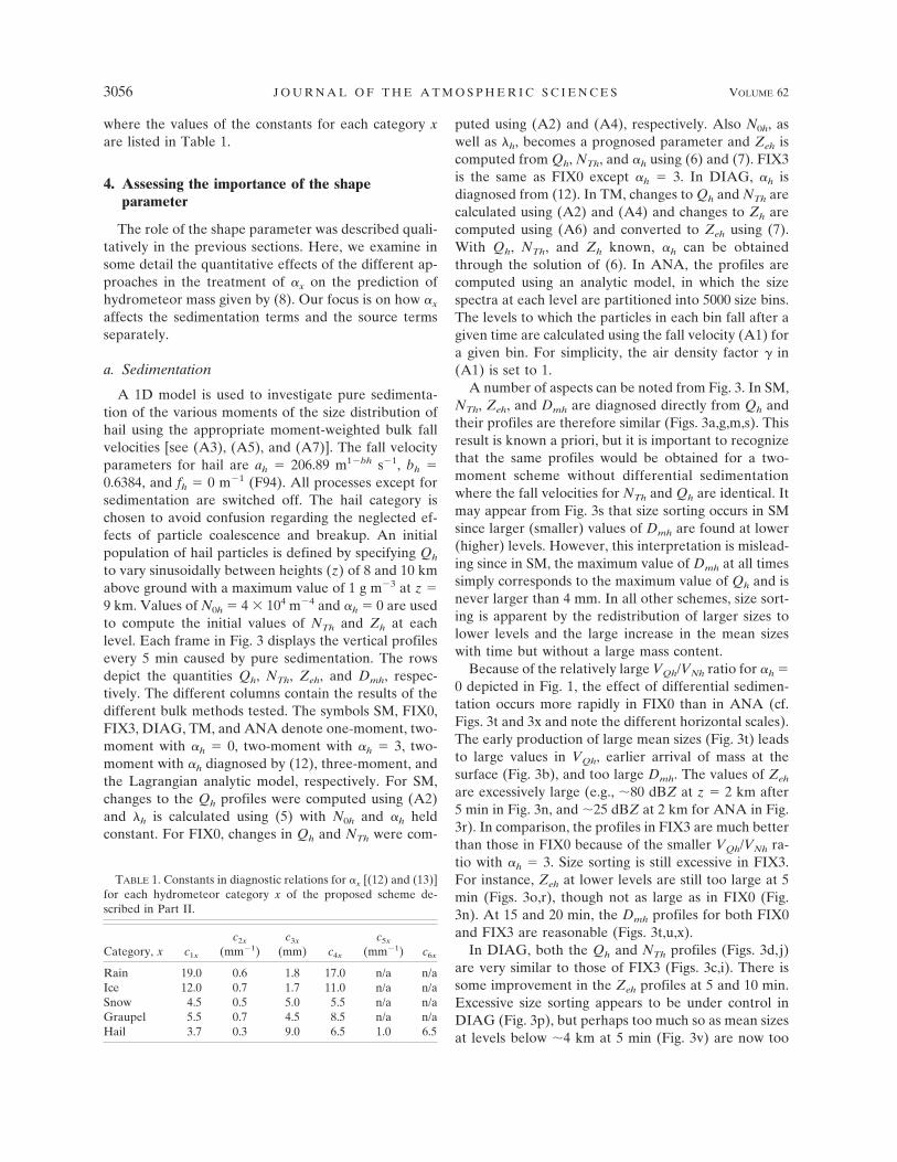
TABLE 1. Constants in diagnostic relations for �x [(12) and (13)]for each hydrometeor category x of the proposed scheme de-scribed in Part II.

Category, x c1x

c2x

(mm�1)c3x

(mm) c4x

c5x

(mm�1) c6x

Rain 19.0 0.6 1.8 17.0 n/a n/aIce 12.0 0.7 1.7 11.0 n/a n/aSnow 4.5 0.5 5.0 5.5 n/a n/aGraupel 5.5 0.7 4.5 8.5 n/a n/aHail 3.7 0.3 9.0 6.5 1.0 6.5


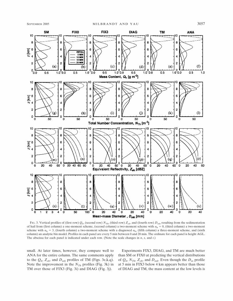
small. At later times, however, they compare well toANA for the entire column. The same comments applyto the Qh, Zeh, and Dmh profiles of TM (Figs. 3e,k,q).Note the improvement in the NTh profiles (Fig. 3k) inTM over those of FIX3 (Fig. 3i) and DIAG (Fig. 3j).

Experiments FIX3, DIAG, and TM are much betterthan SM or FIX0 at predicting the vertical distributionsof Qh, NTh, Zeh, and Dmh. Even though the Dm profileat 5 min in FIX3 below 4 km appears better than thoseof DIAG and TM, the mass content at the low levels is

FIG. 3. Vertical profiles of (first row) Qh, (second row) NTh, (third row) Zeh, and (fourth row) Dmh resulting from the sedimentationof hail from (first column) a one-moment scheme, (second column) a two-moment scheme with �h � 0, (third column) a two-momentscheme with �h � 3, (fourth column) a two-moment scheme with a diagnosed �h, (fifth column) a three-moment scheme, and (sixthcolumn) an analytic bin model. Profiles in each panel are every 5 min between 0 and 20 min. The ordinate for each panel is height AGL.The abscissa for each panel is indicated under each row. (Note the scale changes in n, s, and t.)


however negligible. At 10 min when there is appre-ciable mass content throughout most of the column,DIAG and TM give slightly better Dm profiles thanFIX3. In general, the effect of sedimentation is similarin FIX3, DIAG, and TM, with the latter (Fig. 3q) yield-ing particularly good agreement in radar reflectivity tothe analytic solution (Fig. 3r).

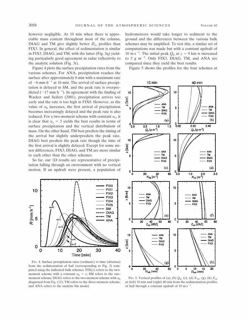
Figure 4 plots the surface precipitation rates from thevarious schemes. For ANA, precipitation reaches thesurface after approximately 8 min with a maximum rateof �6 mm h�1 at 16 min. The arrival of surface precipi-tation is delayed in SM, and the peak rate is overpre-dicted (�17 mm h�1). In agreement with the finding ofWacker and Seifert (2001), precipitation arrives tooearly and the rate is too high in FIX0. However, as thevalue of �h increases, the first arrival of precipitationbecomes increasingly delayed and the peak rate is alsoreduced. For a two-moment scheme with constant �x, itis clear that �x � 3 yields the best results in terms ofsurface precipitation and the vertical distribution ofmass. On the other hand, TM best predicts the timing ofthe arrival but slightly underpredicts the peak rate.DIAG best predicts the peak rate though the time ofthe first arrival is slightly delayed. Except for some mi-nor differences, FIX3, DIAG, and TM are more similarto each other than the other schemes.

So far, our 1D results are representative of precipi-tation falling through an environment with no verticalmotion. If an updraft were present, a population of

hydrometeors would take longer to sediment to theground and the differences between the various bulkschemes may be amplified. To test this, a similar set ofcomputations was made but with a constant updraft of10 m s�1. The initial peak Qh at z � 9 km is increasedto 5 g m�3. Only FIX3, DIAG, TM, and ANA arecompared since they yield the best results.

Figure 5 shows the profiles for the four schemes at

FIG. 4. Surface precipitation rates (ordinate) vs time (abscissa)from the sedimentation of hail (corresponding to Fig. 3) com-puted using the indicated bulk schemes. FIX(x) refers to the two-moment scheme with a constant �h � x; SM refers to the one-moment scheme; DIAG refers to the two-moment scheme with �h

diagnosed from Eq. (12); TM refers to the three-moment scheme;and ANA refers to the analytic bin model.

FIG. 5. Vertical profiles of (a), (b) Qh, (c), (d) NTh, (g), (h) Zeh

at (left) 10 min and (right) 40 min from the sedimentation profilesof hail through a constant updraft of 10 m s�1.


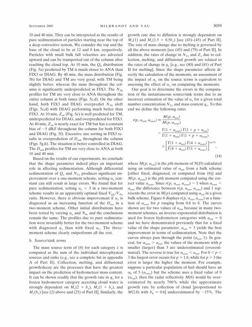
10 and 40 min. They can be interpreted as the results ofpure sedimentation of particles starting near the top ofa deep convective system. We consider the top and thebase of the cloud to be at 12 and 0 km, respectively.Particles with small bulk fall velocities are advectedupward and can be transported out of the column afterreaching the cloud top. At 10 min, the Qh distribution(Fig. 5a) predicted by TM is much closer to ANA thanFIX3 or DIAG. By 40 min, the mass distribution (Fig.5b) for DIAG and TM are very good, with TM beingslightly better, whereas the mass throughout the col-umn is significantly underpredicted in FIX3. The NTh

profiles for TM are very close to ANA throughout theentire column at both times (Figs. 5c,d). On the otherhand, both FIX3 and DIAG overpredict NTh aloft(Figs. 5c,d) with DIAG performing much better thanFIX3. At 10 min, Zeh (Fig. 5e) is well predicted for TM,underpredicted for DIAG, and overpredicted for FIX3.At 40 min, Zeh is nearly exact for TM but has a constantbias of �5 dBZ throughout the column for both FIX3and DIAG (Fig. 5f). Excessive size sorting in FIX3 re-sults in overprediction of Dmh throughout the column(Figs. 5g,h). The situation is better controlled in DIAG.The Dmh profiles for TM are very close to ANA at both10 and 40 min.

Based on the results of our experiments, we concludethat the shape parameter indeed plays an importantrole in affecting sedimentation. Although differentialsedimentation of Qx and NTx produces significant im-provement over a one-moment scheme, setting �x con-stant can still result in large errors. We found that forpure sedimentation, setting �x � 3 in a two-momentscheme results in an apparently optimal fixed VQx/VNx

ratio. However, there is obvious improvement if �x isdiagnosed as an increasing function of the Dmx in atwo-moment scheme. Other initial distributions havebeen tested by varying �x and N0x and the conclusionsremain the same. The profiles due to pure sedimenta-tion were invariably better for the two-moment schemewith diagnosed �x than with fixed �x. The three-moment scheme clearly outperforms all the rest.

b. Source/sink terms

The mass source term of (8) for each category x iscomputed as the sum of the individual microphysicalsources and sinks (e.g., see a complete list in appendixA of Part II). Collection, melting, and diffusionalgrowth/decay are the processes that have the greatestimpact on the prediction of hydrometeor mass content.It can be shown readily that the growth rate in qx for afrozen hydrometeor category accreting cloud water isstrongly dependent on Mx(2 � bx), Mx(1 � bx), andMx(bx) [see (2) above and (25) of Part II]. Similarly, the

growth rate due to diffusion is strongly dependent onMx(1) and Mx(1.5 � 0.5bx) [see (43)–(45) of Part II].The rate of mass change due to melting is governed byall the above moments [see (45) and (79) of Part II]. Inaddition, the rates of change in NTx and Zx due to col-lection, melting, and diffusional growth are related tothe rates of change in qx [e.g., see (80) and (81) of PartII for melting]. Since the shape parameter affects di-rectly the calculation of the moments, an assessment ofthe impact of �x on the source terms is equivalent toassessing the effect of �x on computing the moments.

Our goal is to determine the errors in the computa-tion of the instantaneous source/sink terms due to anincorrect estimation of the value of �x for a given totalnumber concentration NTx and mass content qx. To thisend we define the following ratio:

r�p, �est, �corr� �M�p, �est�

M�p, �corr�

��1 � �corr� ��1 � p � �est�

��1 � �est� ��1 � p � �corr�

× ��1 � �est� ��4 � �corr�

��4 � �est� ��1 � �corr�� p�3�

,

�14�

where M(p, �est) is the pth moment of N(D) calculatedusing an estimated value of �est from a bulk scheme[either fixed, diagnosed, or computed from (6)] andM(p, �corr) is the pth moment computed using the cor-rect value �corr. Since r(p, �est, �corr) � 1 when �corr ��est, the difference between r(p, �est, �corr) and 1 rep-resents the error in M(p) computed using �est in a givenbulk scheme. Figure 6 displays r(p, �est, �corr) as a func-tion of �corr for p ranging from 0.6 to 6. The curvesshown are for two values of �est because in many two-moment schemes, an inverse-exponential distribution isused for frozen hydrometeor categories with �est � 0and we have demonstrated previously that for a fixedvalue of the shape parameter, �est � 3 yields the bestimprovement in terms of sedimentation. Note that thecurves always pass through the point (�est, 1). In gen-eral, for �corr � �est, the values of the moments with psmaller (larger) than 3 are underestimated (overesti-mated). The reverse is true for �corr � �est. For 0 � p �3 the largest error occurs for p � 1.6, while for p � 3 theerror is larger the higher the moment. For example,suppose a particular population of hail should have an�h of 5 (�corr) but the scheme uses a fixed value of 0(�est), then the radar reflectivity M(6) would be over-estimated by nearly 700% while the approximategrowth rate by collection of cloud [proportional toM(2.6) with bh � 0.6] underestimated by �15%. The


same effect occurs if �est � 3 but �corr � 5. In this caseM(6) is overestimated by �42% while M(2.6) underes-timated by �3%. However, if � is fixed at 3 and its truevalue should be 0, M(2.6) would be overestimated by�15%.

To further examine the role of � on the source terms,vertical profiles of M(1.6) and M(2.6) [i.e. Mx(1 � bx)and Mx(2 � bx) for bh � 0.6] after sedimentation of aninitial population of hail particles, identical to the setupshown in Fig. 5, were calculated using the various bulkapproaches as well as the analytic model. The momentsM(1.6) and the M(2.6) are related to the largest and the

smallest errors in the instantaneous growth rate of hail,respectively. To separate the effect of sedimentationfrom the computation of the source terms, the profilesof Qh, NTh, and Zh, due to pure sedimentation in theanalytic model, were used to calculate N0h, �h, and �h inthe various bulk schemes in the same manner describedin section 2. The calculated parameters at various timeswere then used to compute M(1.6) and M(2.6). For theanalytic model, the moments were obtained by sum-ming Dp

i NTi�D over all bins with NTi being the numberof particles in bin i with diameter Di and �D is the binwidth. The ratios of Mh(p)_bulk/Mh(p)ana were thencomputed.

The profiles of Mh(p)_bulk/Mh(p)ana for p � 1.6 andp � 2.6 after 2 and 8 min, along with the correspondingprofiles for �h in a given scheme, are shown in Fig. 7.These early times are chosen for the following reason.Size sorting from sedimentation quickly produces nar-row particle spectra at all levels after only a few min-utes. In a full simulation, other processes may also beoccurring which maintain a broad spectrum. Thereforeit is important to investigate also situations with rela-tively broad spectra. For pure sedimentation, these situ-ations occur only at early times at the mid- and upperlevels. At 2 min, size sorting is only moderate betweenz � 8.0 and 10.5 km and the size spectra, characterizedby the low values of � for TM (Fig. 7c), are broad.Below z � 8.0 km at 2 min and at most levels at or after8 min, size sorting is well advanced and the size spectraare relatively narrow. The moment ratio Mh(p)_bulk/Mh(p)ana is a measure of the accuracy in calculating thepth moment relative to the analytic solution. Valuessmaller (larger) than 1 for a particular bulk schemeimply under- (over-) prediction of the magnitude of themoment.

At 2 min, SM (Figs. 7a,b) underpredicts the two mo-ments above 9 km and greatly overpredicts them below.The results for FIX0 are generally better with the mo-ment ratio always less than 1.00 but never below 0.50for M(1.6) or 0.80 for M(2.6). For FIX3, the curves forthe moment ratio shifted to the right with an underes-timation of �20% for M(0.6) and �10% for M(2.6) atlower levels but an overestimation at higher levels.DIAG behaves similarly to FIX3 above 8.5 km but theunderestimation is greatly reduced below. The best re-sults occur in TM, particularly for the p � 2.6 momentratio, which is close to 1 throughout the column (Fig.7b). The behavior of the curves at 8 min (Figs. 7d,e) isconsistent with those at 2 min; TM performs the best,followed by DIAG, FIX3, FIX0, and SM in descendingorder of performance.

The accurate prediction of the source terms is closelyrelated to the accurate prediction of the width of the

FIG. 6. Ratios of r(p, �est, �corr) (see text) vs �corr for (a) �est �0 and (b) �est � 3 for various pth moments. Insets are magnifica-tions of the panel.


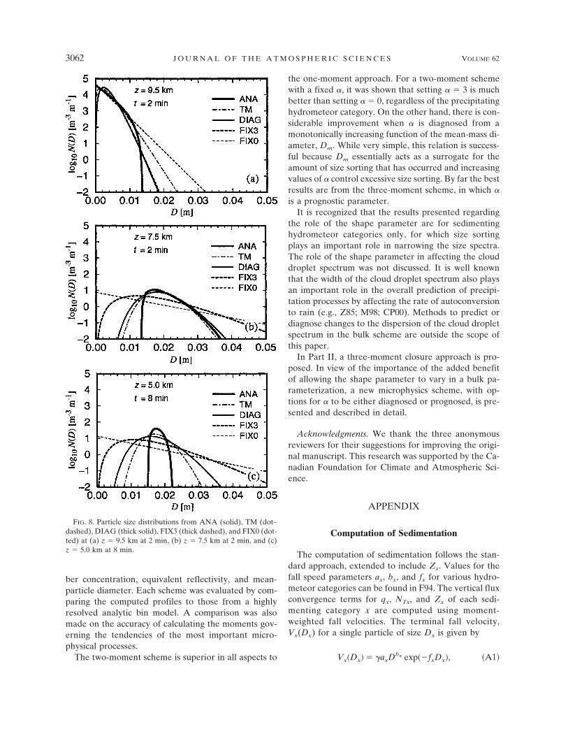
particle size distribution. In Fig. 8, the size spectra atthree different levels and at two different times aredisplayed. For the calculation of the M(1.6) and M(2.6)moments, it is important to predict accurately the sizespectra near the peak of the distribution. For exampleat 2 min and at z � 9.5 km (Fig. 8a), FIX3, DIAG, andTM overpredict the concentration in the diameterrange from �0.002 to 0.006 m, while FIX0 underpre-dicts. This accounts for the overprediction of the mo-ment M(1.6) in FIX3, DIAG, and TM, but an under-prediction in FIX0 (Fig. 7a). At z � 7.5 km and 2 min(Fig. 8b), TM and DIAG predict well the concentrationin the diameter range 0.014–0.028 m surrounding thepeak, as a result the moment M(1.6) in these twoschemes shows excellent agreement with the analyticsolution (Fig. 7a). The underprediction of the concen-tration in FIX3 and FIX0 in the same diameter range isreflected in the underprediction of the 1.6th moment.In the case of the well sorted and thus narrow distribu-tion at 5 km and 8 min (Fig. 8c), the spectra of FIX0 andFIX3 are much broader than the analytic distributionresulting in underestimation of the concentrationaround the modal diameter (�0.019 m) as well as the

moments M(1.6) and M(2.6) (Figs. 7d,e). The distribu-tion is better in DIAG, being narrower and with ahigher concentration around the modal diameter, but itis not as good as in TM, which has a high value for �(Fig. 7f). Although still broader than the analytic spec-trum, the size distribution of TM yields excellentM(1.6) and M(2.6) as depicted in Figs. 7d,e.

5. Conclusions

Given the increasing importance of bulk microphys-ics parameterizations in operational weather predictionand research mesoscale models, it is important to havean understanding of the strengths and limitations ofvarious approaches in order to most appropriately de-velop detailed yet computationally efficient schemes. Adiagnostic equation for the spectral shape parameter �of the gamma size distribution, based on the mean-particle size, has been introduced. Comparisons weremade between a one-moment, two-moment (with pre-scribed and diagnosed values of �), and a three-mo-ment scheme to study the effect of pure sedimentationon the vertical distribution of mass content, total num-

FIG. 7. Vertical profiles of the ratios of M(2.6) computed by various bulk schemes to M(2.6) computed from the (left) analytic modelafter (top) 2 min and (bottom) 8 min and corresponding profiles of � from (right) the bulk schemes. The bulk schemes shown are thethree-moment (dot–dashed), two-moment with � diagnosed from Eq. (12) (thick solid), two-moment with a fixed � � 3 (thick dashed),two-moment with a fixed � � 0 (thin dashed), and one-moment (dotted) schemes.


ber concentration, equivalent reflectivity, and mean-particle diameter. Each scheme was evaluated by com-paring the computed profiles to those from a highlyresolved analytic bin model. A comparison was alsomade on the accuracy of calculating the moments gov-erning the tendencies of the most important micro-physical processes.

The two-moment scheme is superior in all aspects to

the one-moment approach. For a two-moment schemewith a fixed �, it was shown that setting � � 3 is muchbetter than setting � � 0, regardless of the precipitatinghydrometeor category. On the other hand, there is con-siderable improvement when � is diagnosed from amonotonically increasing function of the mean-mass di-ameter, Dm. While very simple, this relation is success-ful because Dm essentially acts as a surrogate for theamount of size sorting that has occurred and increasingvalues of � control excessive size sorting. By far the bestresults are from the three-moment scheme, in which �is a prognostic parameter.

It is recognized that the results presented regardingthe role of the shape parameter are for sedimentinghydrometeor categories only, for which size sortingplays an important role in narrowing the size spectra.The role of the shape parameter in affecting the clouddroplet spectrum was not discussed. It is well knownthat the width of the cloud droplet spectrum also playsan important role in the overall prediction of precipi-tation processes by affecting the rate of autoconversionto rain (e.g., Z85; M98; CP00). Methods to predict ordiagnose changes to the dispersion of the cloud dropletspectrum in the bulk scheme are outside the scope ofthis paper.

In Part II, a three-moment closure approach is pro-posed. In view of the importance of the added benefitof allowing the shape parameter to vary in a bulk pa-rameterization, a new microphysics scheme, with op-tions for � to be either diagnosed or prognosed, is pre-sented and described in detail.

Acknowledgments. We thank the three anonymousreviewers for their suggestions for improving the origi-nal manuscript. This research was supported by the Ca-nadian Foundation for Climate and Atmospheric Sci-ence.

APPENDIX

Computation of Sedimentation

The computation of sedimentation follows the stan-dard approach, extended to include Zx. Values for thefall speed parameters ax, bx, and fx for various hydro-meteor categories can be found in F94. The vertical fluxconvergence terms for qx, NTx, and Zx of each sedi-menting category x are computed using moment-weighted fall velocities. The terminal fall velocity,Vx(Dx) for a single particle of size Dx is given by

Vx�Dx� � axDbx exp��fxDx�, �A1�

FIG. 8. Particle size distributions from ANA (solid), TM (dot–dashed), DIAG (thick solid), FIX3 (thick dashed), and FIX0 (dot-ted) at (a) z � 9.5 km at 2 min, (b) z � 7.5 km at 2 min, and (c)z � 5.0 km at 8 min.


where � � ( 0/ )1/2 is the density correction factor, with 0 being the surface air density and the air density.For each category x, the change in qx due to sedimen-tation is given by the vertical flux convergence for fall-ing particles

qx

t �SEDI�

1�

�qxVQx�

z, �A2�

where the mass-weighted fall speed is given by

VQx �

�0

�

Vx�Dx�mx�Dx�Nx�Dx� dDx

�0

�

mx�Dx�Nx�Dx� dDx

� ax

��1 � dx � �x � bx�

��1 � dx � �x�

�x�1�dx��x�

��x � fx��1�dx��x�bx�.

�A3�

Similarly, the change in NTx due to sedimentation is

NTx

t �SEDI�

�NTxVNx�

z. �A4�

Here, the concentration-weighted fall speed, ratherthan the mass-weighted fall speed, is used:

VNx �

�0

�

Vx�Dx�Nx�Dx� dDx

�0

�

Nx�Dx� dDx

� ax

��1 � �x � bx�

��1 � �x�

�x�1��x�

��x � fx��1��x�bx�.

�A5�

Likewise, changes to Zx due to sedimentation are cal-culated by

Zx

t �SEDI�

�ZxVZx�

z, �A6�

where

VZx �

�0

�

D6Vx�Dx�Nx�Dx� dDx

�0

�

D6Nx�Dx� dDx

� ax

��1 � dx � �x � bx�

��1 � dx � �x�

�x�1�dx��x�

��x � fx��1�dx��x�bx�.

�A7�

Generally, VZx is larger than VQx, which in turn is largerthan VNx (except for rain with small values of �r). Theexistence of different bulk fall velocities for the differ-ent moments creates potential numerical problems in adiscretized model since, for instance, Zx can arrive at alower level before qx and likewise qx can arrive beforeNTx. This must be treated with some care since a levelmust never contain a nonzero value for one momentand a value of zero for another. It was found that simplysetting all values to zero whenever there is zero value ineither one or two variables (and adding the mass qx

back to water vapor, q�, to conserve the total mass)handles this problem quite adequately. A small quan-tity of hydrometeor mass can be lost at the top of avertical profile, but this is a negligible amount. Anotherpossible solution to this problem is simply to use thesame bulk fall velocity for the sedimentation of all ofthe prognostic variables. However, the use of differentfall velocities for the different moments results in im-portant differences to the vertical distribution of thequantities, which is an important benefit of multimo-ment schemes (discussed in section 2).

Equations (A2), (A4), and (A6) are solved by usinga forward-in-time and upstream-in-space finite differ-ence scheme in the paper. The time step is 2.5 s and thevertical grid size is 153 m.

REFERENCES

Cheng, L., and M. English, 1983: A relationship between hailstoneconcentration and size. J. Atmos. Sci., 40, 204–213.

Cohard, J.-M., and J.-P. Pinty, 2000: A comprehensive two-moment warm microphysical bulk scheme. I: Description andtests. Quart. J. Roy. Meteor. Soc., 126, 1815–1842.

Cotton, W. R., G. J. Tripoli, R. M. Rauber, and E. A. Mulvihill,1986: Numerical simulation of the effects of varying ice crys-tal nucleation rates and aggregation processes on orographicsnowfall. J. Climate Appl. Meteor., 25, 1658–1680.

Feingold, G., R. L. Walko, B. Stevens, and W. R. Cotton, 1998:Simulations of marine stratocumulus using a new microphysi-cal parameterization. Atmos. Res., 47-48, 505–528.

Ferrier, B. S., 1994: A two-moment multiple-phase four-class bulkice scheme. Part I: Description. J. Atmos. Sci., 51, 249–280.

——, W.-K. Tao, and J. Simpson, 1995: A two-moment multiple-phase four-class bulk ice scheme. Part II: Simulations of con-vective storms in different large-scale environments and com-parisons with other bulk parameterizations. J. Atmos. Sci., 52,1001–1033.

Ivanova, D., D. L. Mitchell, W. P. Arnott, and M. Poellot, 2001: AGCM parameterization for bimodal size spectra and ice massremoval rates in mid-latitude cirrus clouds. Atmos. Res., 59-60, 89–113.

Kessler, E., 1969: On the Distribution and Continuity of WaterSubstance in Atmospheric Circulation. Meteor. Monogr., No.32, Amer. Meteor. Soc., 84 pp.

Kong, F., and M. K. Yau, 1997: An explicit approach to micro-physics in MC2. Atmos. Ocean., 33, 257–291.


Lin, Y.-L., R. D. Farley, and H. D. Orville, 1983: Bulk parameter-ization of the snow field in a cloud model. J. Climate Appl.Meteor., 22, 1065–1092.

Marshall, J. S., and W. McK. Palmer, 1948: The distribution ofraindrops with size. J. Atmos. Sci., 5, 165–166.

Meyers, M. P., R. L. Walko, J. Y. Harrington, and W. R. Cotton,1997: New RAMS cloud microphysics. Part II: The two-moment scheme. Atmos. Res., 45, 3–39.

Milbrandt, J. A., and M. K. Yau, 2005: A multimoment bulk mi-crophysics parameterization. Part II: A proposed three-moment closure and scheme description. J. Atmos. Sci., 62,3065–3081.

Murakami, M., 1990: Numerical modeling of dynamical and mi-crophysical evolution of an isolated convective cloud—The19 July 1981 CCOPE cloud. J. Meteor. Soc. Japan, 68, 107–128.

Sekhon, R. S., and R. C. Srivastava, 1970: Snow spectra and radarreflectivity. J. Atmos. Sci., 27, 299–307.

Srivastava, R. C., 1978: Parameterization of raindrop size distri-butions. J. Atmos. Sci., 35, 108–117.

Uijlenhoet, R., M. Steiner, and J. A. Smith, 2003: Variability ofraindrop size distributions in a squall line and implications forradar rainfall estimation. J. Hydrometeor., 4, 43–61.

Ulbrich, C. W., 1983: Natural variations in the analytical form ofthe raindrop size distribution. J. Climate Appl. Meteor., 22,1764–1775.

Wacker, U., and A. Seifert, 2001: Evolution of rain water profilesresulting from pure sedimentation: Spectral vs. parameter-ized description. Atmos. Res., 58, 19–39.

Waldvogel, A., 1974: The N0 jump of raindrop spectra. J. Atmos.Sci., 31, 1067–1078.

Yu, W., L. Garand, and A. P. Dastoor, 1997: Evaluation of modelclouds and radiation at 100 km scale using GOES data. Tel-lus, 49A, 246–262.

Ziegler, C. L., 1985: Retrieval of thermal and microphysical vari-ables in observed convective storms. Part 1: Model develop-ment and preliminary testing. J. Atmos. Sci., 42, 1497–1509.


a multimoment bulk microphysics parameterization. part i

Documents