a multilevel stochastic collocation … is a template for the application of multigrid to...

A MULTILEVEL STOCHASTIC COLLOCATION ALGORITHM FOROPTIMIZATION OF PDES WITH UNCERTAIN COEFFICIENTS

D. P. KOURI ∗

Abstract. In this work, we apply the MG/OPT framework to a multilevel-in-sample-spacediscretization of optimization problems governed by PDEs with uncertain coefficients. The MG/OPTalgorithm is a template for the application of multigrid to deterministic PDE optimization problems.We employ MG/OPT to exploit the hierarchical structure of sparse grids in order to formulate amultilevel stochastic collocation algorithm. The algorithm is provably first-order convergent understandard assumptions on the hierarchy of discretized objective functions as well as on the optimizationroutines used as pre- and post-smoothers. We present explicit bounds on the total number of PDEsolves and an upper bound on the error for one V-cycle of the MG/OPT algorithm applied to a linearquadratic control problem. We provide numerical results that confirm the theoretical bound on thenumber of PDE solves and show a dramatic reduction in the total number of PDE solves requiredto solve these optimization problems when compared with standard optimization routines applied tothe same problem.

Key words. PDE Optimization, Multilevel, Uncertainty Quantification, Sparse Grids

AMS subject classifications. 49M15, 65K05, 65N35, 90C15

1. Introduction. The numerical solution of partial differential equation (PDE)constrained optimization problems with uncertain coefficients is computationally ex-pensive because of typically high-dimensional stochastic representations of the PDEsolution. This work applies the MG/OPT algorithm [33] to solve the optimizationproblem

Minimizez∈Z

J(z) = J(u(z), z),

where Z is a reflexive Hilbert space, U is a Banach space, and u = u(z) ∈ U is

the solution of a PDE with uncertain coefficients. We discretize J(z) in the samplespace using a hierarchical sparse grid collocation discretization [27]. We demonstratethat applying MG/OPT to this hierarchy of semi-discretized optimization problems

may reduce the number of PDE solves required to obtain a minimizer of J(z) whencompared with other standard optimization algorithms.

The MG/OPT algorithm is an optimization-theoretic multigrid approach to solv-ing PDE-constrained optimization problems [33, 30]. MG/OPT is a template whichallows for user-defined optimization routines, discretizations, and intergrid transferoperators [33, 30]. Moreover, MG/OPT generalizes the full approximation scheme(FAS) [25] to optimization and has traditionally been applied to a hierarchy of spatialdiscretizations for the state and design variables. In this work, we apply the ideas ofMG/OPT to a hierarchy of stochastic discretizations.

Globalized with a line search, MG/OPT is provably convergent [33, 34]. At eachlevel, MG/OPT is analogous to a V-cycle (or more general cycles) of multigrid. Asin traditional multigrid, each level of MG/OPT requires pre- and post-smoothing.These smoothing steps correspond to performing a finite number of iterations of anoptimization algorithm [33]. Recently, the authors of [21, 22, 23, 24] have developed a

∗Mathematics & Computer Science Division, Argonne National Laboratory, 9700 South CassAvenue, Building 240, Argonne, IL 60439-4844. E-mail: [email protected]. This author wassupported by the U.S. Department of Energy, Office of Science, Advanced Scientific ComputingResearch, under Contract DE-AC02-06CH11357.

1

2 D. P. KOURI

recursive trust-region algorithm that accelerates the trust-region step using multigridcorrection. Similarly, [47] has developed a line-search approach to multigrid opti-mization. Both of the multilevel trust-region and line-search algorithms are provablyconvergent and do not require pre- and post-smoothing.

Aside from MG/OPT and its adaptations, spatial multigrid has been appliedto optimization problems governed by deterministic PDEs in [44, 8, 7, 10, 11, 12]by using multigrid solvers on the optimality system. We note that simply applyingmultigrid to the optimality system need not result in a minimizer since multigrid seeksonly a stationary point of the optimality system [30]. This pitfall is circumvented byincluding target functions in the multigrid formulation. These ideas are extendedto problems governed by PDEs with uncertain coefficients in [13, 14, 15]. Thoseworks focus on multigrid in space, however, and do not consider multilevel samplingschemes. Unlike these multigrid algorithms for PDE-optimization with uncertaincoefficients, the algorithm presented in this paper provides a multilevel-in-sample-space optimization routine. Moreover, one can incorporate existing spatial multigridalgorithms within the MG/OPT framework to solve the sparse-grid subproblems.

In Section 2, we present the problem formulation for the example problems con-sidered in this paper. The problem formulation resembles standard quadratic controlor least-squares type PDE-optimization. In Section 3, we review stochastic colloca-tion and discuss hierarchical sparse-grid techniques. In Section 4 we extend MG/OPTto handle optimization of uncertain PDEs, and in Section 5 we prove the first-orderconvergence of MG/OPT. In Section 6, we present explicit upper bounds on V-cycleerror and computational work. In Section 7, we demonstrate the power and efficiencyof MG/OPT for stochastic collocation through numerical examples. In Section 8, wepresent conclusions and future work.

The following notation and conventions are employed throughout this paper. Kdenotes the finest level of sparse grid, and 1 always refers to the coarsest level of sparsegrid. The index k denotes the intermediate levels of sparse grid (i.e., k = 1, 2, . . . ,K).

2. Problem Formulation. Let D ⊂ Rd, d = 1, 2, 3, denote the physical domainand Γ ⊆ RM denote the finite sample space. The sample space Γ is endowed with theprobability density ρ : Γ→ [0,∞) and satisfies

Γ =

M∏m=1

[am, bm] and ρ(y) =

M∏m=1

ρm(ym)

with am < bm and ρm : [am, bm]→ [0,∞) for m = 1, . . . ,M . Such finite-dimensionalprobability spaces satisfy the finite-dimensional noise assumption [1] and typicallyresult from Karhunen-Loeve or polynomial chaos expansions. Let V = V(D) denote aBanach space of deterministic functions with domain D, and let Z = Z(D) denote areflexive Hilbert space of deterministic functions with domain D. V is the determin-istic state space and Z is the control space. The control space is deterministic; thismodels the situation when one must determine a control prior to observing the stateof the physical system. The governing PDEs in this work have the form

A(y)u(y) + N(u(y), y) = F(z, y) ∀ y ∈ Γ, (2.1)

where A : Γ → L(V,V∗), N : V × Γ → V∗, and F : Z × Γ → V∗. Now, let theHilbert space W, C ∈ L(V,W), and w ∈ W be given. The prototypical example forPDE-constrained optimization is the quadratic control problem

minz∈Z

J(z) =1

2

∫Γ

ρ(y)‖Cu(z; y)− w‖2W dy +α

2‖z‖2Z , (2.2)

MULTILEVEL STOCHASTIC COLLOCATION FOR OPTIMIZATION 3

where u(z; y) = u(y) ∈ V solves (2.1) almost surely in Γ. The solution of this opti-mization problem can be approximated by sampling schemes such as Monte Carlo [31]and stochastic collocation [1, 37, 36, 48] or by projection schemes such as stochasticGalerkin [2, 3] and polynomial chaos [49, 17].

To simplify the analysis in this section, we focus on the quadratic control problem(2.2). The algorithm presented in this paper also applies to more general objectivefunctions, although the analysis is typically more complicated [27].

The solution of (2.1) is a mapping y 7→ u(y) : Γ → V and is assumed to havefinite pth moment for some fixed p ∈ [1,∞); that is, u ∈ Lpρ(Γ;V), where

Lpρ(Γ;V) = {v : Γ→ V : v strongly measurable,

∫Γ

ρ(y)‖v(y)‖pV dy <∞}.

To sample y 7→ u(y), we further assume that u ∈ U = C0ρ(Γ;V), where

C0ρ(Γ;V) = {v : Γ→ V : v continuous, sup

y∈Γρ(y)‖v(y)‖V <∞}

which ensures that point evaluations of y 7→ u(y) are possible. Furthermore, forthe objective function to be well-defined, we require that C0

ρ(Γ;V) be continuouslyembedded in L2

ρ(Γ;V).Assumption 2.1. The inclusion C0

ρ(Γ;V) ⊂ L2ρ(Γ;V) holds. Moreover, for each

z ∈ Z the state equation (2.1) has a unique solution u(z; ·) ∈ C0ρ(Γ;V) satisfying

‖u(z; ·)‖L2ρ(Γ;V) ≤ c‖u(z; ·)‖C0

ρ(Γ;V) for some c > 0.The algorithm described in this paper requires gradient information. We use

adjoints to derive the gradient, ∇J(z). To ensure differentiability, we require thefollowing assumption.

Assumption 2.2. For every y ∈ Γ, the functions v 7→ N(v, y) : V → V∗ andz 7→ F(z, y) : Z → V∗ are Frechet differentiable with Frechet derivatives N′(u, y) andF′(z, y), respectively. Moreover, the mapping z 7→ u(z; ·) : Z → C0

ρ(Γ;V) is Frechetdifferentiable, and the derivative v = u′(z; ·)δz satisfies

A(y)v(y) + N′(u(y), y)v(y) = F′(z, y)δz ∀ y ∈ Γ.

Additionally, the adjoint equation

A(y)∗p(y) + N′(u(y), y)∗p(y) = −C∗(Cu(z; y)− w) ∀ y ∈ Γ (2.3)

has a unique solution p ∈ C0ρ(Γ;V).

If Assumptions 2.1 and 2.2 hold, then the gradient of the objective function J(z) is

∇J(z) = αz −∫

Γ

ρ(y)F′(z, y)∗p(y) dy.

3. Hierarchical Sampling Approaches: Sparse Grid Collocation. Multi-level and adaptive Monte Carlo methods for the solution of the unconstrained stochas-tic programming problems are presented in [5, 16]. Furthermore, adaptive sparse-gridcollocation methods are developed in [27, 28]. In this section, we review sparse grids[19, 4, 20, 42] with the goal of exposing their hierarchical nature.

We approximate the expected value in (2.2) using sparse-grid quadrature. Sparse-grid quadrature exhibits rapid convergence when y 7→ ‖Cu(y) − w‖2W is sufficiently

4 D. P. KOURI

smooth. Tensor products of 1D quadrature operators are the foundation for sparse-grid quadrature. Let {Ej,m}∞j=1 denote a sequence of 1D quadrature operators definedfor continuous functions on [am, bm]. We assume that the degree of polynomial exact-ness for Ej,m is djm − 1, where {djm}∞j=1 ⊂ N is monotonically increasing. Associatedwith each Ej,m is a finite set of knots Nj,m ⊂ Γm. For example, Ej,m can be Gaussian,Hermite, or Newton-Cotes quadrature operators.

To construct the sparse grid operator, we define the one-dimensional differences

∆1,m = E1,m and ∆j,m = Ej,m − Ej−1,m j ≥ 2.

Then Ej,m =∑ji=1 ∆j,m. Let I ⊂ NM+ where N+ = {1, 2, · · · }. The general sparse-

grid quadrature operator is

EI =∑i∈I

∆i1,1 ⊗ · · · ⊗∆iM ,M . (3.1)

In order to maintain the telescoping sum property described above, the multi-indexset, I, must satisfy the following property: If i = (i1, . . . , iM ) ∈ I and j = (j1, . . . , jM )is such that jm ≤ im for all m = 1, . . . ,M , then j ∈ I. A multi-index set satisfyingthis property is called admissible [20]. Each admissible multi-index set I produces aset of points NI ⊂ Γ called a sparse grid.

The general sparse-grid operator (3.1) can be written as a linear combination oftensor products of 1D quadrature operators by using the combination technique [19]:

EI =∑i∈I

( ∑j∈{0,1}M

(−1)|j|1χI(i + j)

)(Ei1,1 ⊗ · · · ⊗ EiM ,M

), (3.2)

where |j|1 = j1 + . . .+ jM and χI(j) = 1 if j ∈ I and zero otherwise. From (3.2), onecan determine the particular form of the sparse grid, NI . Define

ϑ(i) =∑

j∈{0,1}M(−1)|j|1χI(i + j).

Then the sparse grid associated with I is

NI =⋃

{i∈I : ϑ(i)6=0}

(Ni1,1 × · · · ×NiM ,M

). (3.3)

Now, suppose {Ik}∞k=1 is a family of admissible multi-index sets satisfying

{(1, · · · , 1)} ⊆ I1 ⊂ I2 ⊂ · · · ⊂ NM+

and the one-dimensional nodes Nj,m are nested (i.e., Nj−1,m ⊂ Nj,m ∀ j). Then,the resulting sparse grids are nested (i.e. Nk = NIk ⊂ Nk+1 = NIk+1

for k = 1, 2, . . .).Nested sparse grids are desirable for computation because they allow for the reuse ofmany computations in the hierarchy of sparse grids.

3.1. Exposing the Hierarchical Sampling Structure. Hierarchies of multi-index sets Ik ⊂ Ik+1 can be generated in a multitude of ways. Some common methodsare full tensor-product and isotropic/anisotropic Smolyak algorithms [42, 36, 1]. Themulti-index sets constructed from the full tensor-product algorithm are defined as

Ik = {i ∈ NM+ : max`=1,...,M

|i` − 1| ≤ (k − 1)}.


On the other hand, the anisotropic Smolyak algorithm employs the multi-index set

Ik = {i ∈ NM+ :

M∑`=1

γ`|i` − 1| ≤ γ∗(k − 1)},

where γ = (γ1, . . . , γM ) is an M-tuple of positive real numbers and γ∗ = min` γ`.Each component of γ determines the relative importance of the associated direction;and, in the case that γ = (1, . . . , 1), we recover the isotropic Smolyak sparse-gridindex set. For both the full tensor-product and Smolyak algorithms, the multi-indexsets create the hierarchy required above. In general, the resulting point sets Nkproduced from the Smolyak algorithm are sparser than those created from the fulltensor-product algorithm. Hence, the Smolyak multi-index sets require fewer solvesof (2.1) to evaluate the discretized objective functions, Jk = JIk .

Now, consider isotropic Smolyak sparse grids, and suppose that the one-dimensionalquadrature points satisfy |Nk,j | = O(2k) for j = 1, . . . ,M . Then, the authors of [19]show that the resulting sparse grids satisfy

Qk = |Nk| = O(2kkM−1).

The growth rate between levels k and k − 1 is given by

qk = Qk/Qk−1 ≈ 2( k

k − 1

)M−1

for k sufficiently large. Asymptotically, as k → ∞, the growth rate is 2, and thelargest growth occurs between levels k = 1 and k = 2, namely, q2 = Q2/Q1 ≈ 2M .In fact, for k = 1, Q1 = 1 independent of the number of dimensions M . Therefore,q2 = Q2 for all M . The growth rate {qk}∞k=1 is a monotonically decreasing sequencein the interval [2, Q2].

A popular choice of 1D quadrature points on [−1, 1] are Clenshaw-Curtis points

Nm,j =

{− cos

(π(i− 1)

dj − 1

): i = 1, . . . , di

}with d1 = 1 and di = 2j−1 + 1 for j > 1. The Clenshaw-Curtis points are nested.Furthermore, these points satisfy the assumptions on growth rate discussed in theprevious paragraph. Therefore, the sequence of growth rates for the sparse grids builton Clenshaw-Curtis nodes is decreasing on [2, Q2].

3.2. Sparse-Grid Collocation. Given an admissible multi-index set I ⊂ NMand the associated quadrature rule EI , the collocation discretization of (2.2) is

minz∈Z

JI(z) =1

2EI[‖Cu(z)− w‖2W

]+α

2‖z‖2Z (3.4)

Note that the evaluation of the quadrature rule EI requires the solution of only theQI = |NI | deterministic, decoupled PDEs

A(yI` )u` + N(u`, yI` ) = F(z, yI` ) ∀ ` = 1, . . . , QI ,

where NI = {yI1 , . . . , yIQI} [27, 28]. This is equivalent to a stochastic collocationdiscretization of (2.1) [27]. The semi-discretized objective function can be written inthe standard quadrature form as

JI(z) =1

2

QI∑`=1

ωI` ‖Cu`(z)− w‖2W +α

2‖z‖2Z ,

6 D. P. KOURI

where ωI` are appropriate sparse-grid quadrature weights. Moreover, if Assump-

tions 2.1 and 2.2 hold, then JI(z) is Frechet differentiable with gradient

∇JI(z) = αz −QI∑`=1

ωI` F′(z, yI` )∗p`.

In the gradient, p` ∈ V solves the decoupled deterministic adjoint equations

A(yI` )∗p` + N(u`, yI` )∗p` = −C∗(Cu` − w) ∀ ` = 1, . . . , QI .

These decoupled adjoint equations are equivalent to a stochastic collocation discretiza-tion of the infinite-dimensional adjoint equation (2.3) [27].

We note that sparse grids typically produce both positive and negative quadratureweights [19]. The presence of negative weights may affect optimization because JI(z)

may not be convex or weakly lower semi-continuous even if J(z) is [27, 26].

3.3. Collocation Error Bounds. The convergence of stochastic collocationhas been extensively studied for elliptic, parabolic, and hyperbolic PDEs. See, forexample, [37, 36, 35, 1, 32]. The standard result applies for both bounded and un-bounded Γ. For simplicity, we assume Γ is bounded. Furthermore, we require thefollowing assumption on the regularity of the solution u of (2.1) with respect tothe parameters y ∈ Γ. For these assumptions, we use the following notation: fory = (y1, . . . , yM ) ∈ Γ, y∗j = (y1, . . . , yj−1, yj+1, . . . , yM ) ∈ Γ∗j =

∏` 6=j Γ`. Further-

more, given u ∈ C0ρ(Γ;V), we consider the function u∗j : Γj → C0

ρ∗j(Γ∗j ;V) to be

defined by (u∗j (ξ))(y∗j ) = u(y1, . . . , yj−1, ξ, yj+1, . . . , yM ), where ρ∗j =

∏` 6=j ρj .

Assumption 3.1. Let Assumptions 2.1 and 2.2 hold. Suppose Γ is bounded, andlet u ∈ C0

ρ(Γ;V) be the solution to (2.1) for fixed z ∈ Z. Then there exists τj > 0such that u∗j : Γj → C0

ρ∗j(Γ∗j ;V) has an analytic extension on the set

Σ(Γj ; τj) = {ξ ∈ C : dist(ξ,Γj) ≤ τj}.

Furthermore, let p ∈ C0ρ(Γ;V) be the solution to (2.3). Then there exists γj > 0 such

that p∗j : Γj → C0ρ∗j

(Γ∗j ;V) has an analytic extension on the set Σ(Γj ; γj).

Similar assumptions to those in Assumption 3.1 can be found in [1, Lem. 3.2],[37, Lem. 3.2], and [36, Lem. 2.3]. For examples of the state equation (2.1) thatsatisfy Assumption 3.1, see [37, 36, 35, 1, 32]. For examples of optimization problems(2.2) for which (2.1) and (2.3) satisfy Assumption 3.1, see [28, 27]. If Assumption 3.1holds, then stochastic collocation provides a convergent approximation scheme. Theconvergence of stochastic collocation depends on the quadrature rules used. In the caseof elliptic PDEs, convergence is proven for isotropic and anisotropic tensor productquadrature built on 1D Gaussian abscissae, as well as isotropic and anisotropic sparse-grid quadrature built on Gaussian and Clenshaw-Curtis abscissae. These results arestated in [1, Thm. 4.1] for tensor products of Gaussian abscissae, in [37, Thm. 3.10,3.11, 3.18, 3.19] for isotropic sparse grids built on Clenshaw-Curtis and Gaussianabscissae, and in [36, Thm. 3.8, 3.13] for anisotropic sparse grids built on Clenshaw-Curtis and Gaussian abscissae. The standard error bound has a specific form that weassume throughout.

Assumption 3.2. Let Assumption 3.1 hold, and let τ = (τ1, . . . , τM ) andγ = (γ1, . . . , γM ). Furthermore, suppose I ⊂ NM+ is an admissible index set with


corresponding sparse grid NI , Q = |NI |. Then, u ∈ C0ρ(Γ;V) solving (2.1) and

p ∈ C0ρ(Γ;V) solving (2.3) satisfy

‖E[u]− EI [u]‖L∞ρ (Γ;V) ≤ C(r(τ ),M)Q−ν(τ ,M) (3.5)

and

‖E[p]− EI [p]‖L∞ρ (Γ;V) ≤ C(r(γ),M)Q−ν(γ,M), (3.6)

respectively. The function r : RM → RM is defined componentwise for j = 1, . . . ,M

by rj(τ) = log(

2τ|Γj | +

√1 + 4τ2

|Γj |2

).

These results are extended to the optimization context for uniformly convexlinear-quadratic optimal control problems in [27]. In this case, if zQ ∈ Z is a first-order necessary point of (3.4) and z∗ ∈ Z is a first-order necessary point of (2.2), thenthe error between zQ and z∗ satisfies the upper bound

‖zQ − z∗‖Z ≤ C(r(γ),M)Q−ν(r(γ),M),

where ν is defined in (3.6).

4. MG/OPT as a Multilevel-in-Sample-Space Optimization Solver. Sim-ilar to classic spatial multigrid, the hierarchy of sparse-grid operators described aboveinduces a hierarchy of (semi-)discretized optimization problems (2.2):

minz∈Z

Jk(z) =1

2

Qk∑i=1

ωki ‖Cui(z)− w‖2W +α

2‖z‖2Z , k = 1, . . . ,K.

Recall that the evaluation of Jk(z) requires the solution of (2.1) at all points in thesparse grid Nk (i.e., Qk = |Nk| PDE solves). MG/OPT applies to this hierarchy ofoptimization problems. In addition, the variants of MG/OPT such as recursive trust-regions [21, 22, 23, 24] and the multilevel line-search approach of [47] also apply to thishierarchy of sparse-grid discretizations, but we restrict our attention to MG/OPT.

Unlike spatial multigrid, the hierarchy of sparse-grid collocation discretizationspaces appears implicitly in the definition of the semi-discretized objective function.That is, the control space is fixed, and ∇Jk(z) ∈ Z for all k. Therefore, the intergridtransfer operators (prolongation and interpolation) of spatial multigrid are triviallythe identity operator. Moreover, for the application of MG/OPT, it is convenient todefine the coarse-grid corrected objective functions

Jk(z) = Jk(z | vk) = Jk(z)− 〈vk, z〉Z for vk ∈ Z.

The MG/OPT algorithm defines vk at each level, but it is always the case that vK = 0.The multilevel sparse grid optimization algorithm is stated in Algorithm 1.

We offer a few comments on the implementation of Algorithm 1. First, Algo-rithm 1 defines one V-cycle of MG/OPT; and, with little modification, one can definemore general cycles such as W-cycles, F-cycles, or cascadic multigrid. Second, thepre- and post-smoothing steps at each level, (4.2) and (4.4), can be computed byapplying a fixed number of iterations of an optimization routine as suggested in [33].Alternatively, Borzi [9, 6] suggests applying the pre- and post-smoothing optimizationroutines until the following sufficient decrease conditions are satisfied:

Jk(zk,1) < Jk(z−k )− ηk,1‖∇J (z−k )‖Z ηk,1 ∈ (0, 1)

Jk(z+k ) < Jk(zk,3)− ηk,2‖∇J (zk,3)‖Z ηk,2 ∈ (0, 1).

8 D. P. KOURI

MG/OPT: z+k = MG/OPT(k, z−k , vk)

if k = 1 thenReturn z+

1 = z−1 + s1 where s1 satisfies

s1 = arg mins∈Z

J1(z−1 + s) = J1(z−1 + s)− 〈v1, (z−1 + s)〉Z . (4.1)

elsePre-Smoothing: Perform T1,k iterations of a convergent optimizationalgorithm to obtain

sk,1 ≈ arg mins∈Z

Jk(z−k + s) = Jk(z−k + s)− 〈vk, (z−k + s)〉Z (4.2)

and update zk,1 = z−k + sk,1.

Coarse Grid Correction: Set vk−1 = vk + (∇Jk−1(zk,1)−∇Jk(zk,1))

and approximately minimize Jk−1(z) = Jk−1(z)− 〈vk−1, z〉Z using

zk,2 = MG/OPT(k − 1, zk,1, vk−1). (4.3)

Line Search: Use a line search to determine λk ≥ 0 which sufficientlyreduces Jk(zk,1 + λ(zk,2 − zk,1)) and set zk,3 = zk,1 + λk(zk,2 − zk,1).Post-Smoothing: Perform T2,k iterations of a convergent optimizationalgorithm to obtain

sk,2 ≈ arg mins∈Z

Jk(zk,3 + s) = Jk(zk,3 + s)− 〈vk, (zk,3 + s)〉Z (4.4)

and return z+k = zk,3 + sk,2.

end

Algorithm 1: Recursive MG/OPT algorithm.

Third, if ∇2Jk(zk,1) exists and is Lipschitz continuous with Lipschitz constant Lk > 0for k = 1, . . . ,K and if ek = (zk,2 − zk,1) is a descent direction, then Borzi [9, 6]suggests the following a priori choice for the line-search parameter λk:

λk = min

{2,

−〈∇Jk(zk,1), ek〉Z〈∇2Jk(zk,1)ek, ek〉Z + Lk‖ek‖2Z

}.

This choice of λk guarantees sufficient decrease in the objective function. In general,Lk is unknown, and λk is computed by using a standard line-search rule such asbacktracking. As noted in [29], the a priori choice λk = 1 as commonly used inthe globalization of Newton’s method may not apply to MG/OPT. Furthermore, thenestedness of the sparse grids Nk implies that no additional PDE solves are requiredwhen computing vk−1. For optimization problem (2.2), vk−1 can be written as

vk−1 = vk +

Qk−1∑i=1

(ωk−1i − ωki )F′(z, yKi )∗pi −

Qk∑i=Qk−1+1

ωki F′(z, yKi )∗pi

where K denotes the finest level of sparse grid, ωki = ωIki denotes the level k sparse-

grid weights, yKi = yIKi denotes the level K sparse-grid points ordered so that

NK = {N1, N2 \N1, . . . , NK \NK−1} = {y11 , . . . , y

1Q1, . . . , yKQK−1+1, . . . , y

KQK},

and pi ∈ V solves the adjoint equation (2.3) at y = yki for i = 1, . . . , Qk.


5. Convergence Analysis for Algorithm 1. The analysis here follows directlyfrom the analysis for MG/OPT in [33, 34]. The author in [9, 6] proves similar resultsusing standard multigrid techniques. The convergence analysis for Algorithm 1 doesnot require restriction and prolongation operators. In fact, this analysis depends onlyon the sparse-grid discretization through the assumptions on the subproblems Jk(z).The results in this section require the following assumptions.

Assumption 5.1. Let K ∈ N be the finest level of sparse-grid hierarchy andassume a minimizer of JK(z) exists. Denote this minimizer by z∗K ∈ Z. Furthermore,let Br(z∗K) = {z ∈ Z : ‖z − z∗K‖Z < r} denote the open ball of radius r > 0 in Z.

1. Jk(z) is twice continuously Frechet differentiable and bounded below for allk = 1, . . . ,K.

2. There exists r > 0 independent of k = 1, . . . ,K such that ∇2Jk(z) ∈ L(Z,Z)is a uniformly positive-definite operator for all z ∈ Br(z∗K) and k = 1, . . . ,K;that is, there exists κk > 0 such that

〈∇2Jk(z)ξ, ξ〉Z ≥ κk‖ξ‖2Z ∀ 0 6= ξ ∈ Z, ∀ z ∈ Br(z∗K). (5.1)

3. The smoothing iteration numbers satisfy

T1,k ≥ 0, T2,k ≥ 0, and T1,k + T2,k > 0 for k = 1, . . . ,K.

4. The optimization routines used in (4.1), (4.2), and (4.4) are first-order con-vergent in the sense that

lim infj‖∇Jk(zj)‖Z = 0.

Assumption 5.1 ensures that the semi-discretized optimization problems at eachlevel k are well-defined. Assumption 5.1.1 ensures that Newton-type methods areapplicable. Assumption 5.1.2 assumes that when close to a solution (basin of attrac-tion), the Hessian operators are positive-definite. This ensures second-order sufficientconditions hold at the minimizer. Assumptions 5.1.3-4 guarantee that Algorithm 1makes progress toward a solution. Under these assumptions, we first prove thateK = zK,2 − zK,1 is a descent direction.

Theorem 5.2. Let Assumption 5.1 hold, and let zK,1 ∈ Br(z∗K). Furthermore,suppose the optimization problem (4.3) is solved to the relative gradient tolerance

‖∇JK−1(zK,2)− vK−1‖Z ≤ γκK−1‖zK,1 − zK,2‖Z with γ ∈ [0, 1). (5.2)

Then eK = zK,2 − zK,1 is a descent direction.Proof. Suppose the approximate solution of (4.3) satisfies (5.2). Then there exists

η ∈ Z such that ‖η‖Z ≤ γκK−1‖zK,2 − zK,1‖Z and

∇JK(zK,1) = ∇JK−1(zK,1)−∇JK−1(zK,2) + η.

Therefore,⟨∇Jk(zK,1), eK

⟩Z

=⟨∇JK−1 (zK,1)−∇JK−1(zK,2) + η, eK

⟩Z

=

⟨∫ 1

0

∇2JK−1 (zK,2 − teK) (−eK) dt, eK

⟩Z

+ 〈η, eK〉Z

≤ −κK−1‖eK‖2Z + ‖η‖Z‖eK‖Z ≤ (γ − 1)κK−1‖eK‖2Z < 0.

10 D. P. KOURI

Hence, eK is a descent direction.The first-order convergence of Algorithm 1 is an easy consequence of Theorem 5.2.Corollary 5.3. Let Assumption 5.1 and inequality (5.2) hold. Furthermore,

let K ∈ N+ denote the finest level of sparse grid. Suppose {z(j)K }∞j=1 ⊂ Z denotes a

sequence of iterations produced by Algorithm 1 with initial guess z(0)K ∈ Z. Then

lim infj‖∇JK(z

(j)K )‖Z = 0.

Proof. If for some j the iterate z(j)K ∈ Br(z∗K), then Theorem 5.2 ensures the

search direction eK is a descent direction, and Theorem 1 of [33] proves the result.

On the other hand, if z(j)K 6∈ Br(z∗K), then the search direction eK need not be a

descent direction. If eK is not a descent direction, then the line-search parameter isλK = 0. In this case, Assumption 5.1.4 (i.e., global convergence of the smoothers)ensures the global convergence of Algorithm 1.

Remark 5.4. Corollary 5.3 also holds if we replace Assumption 5.1.2 with theassumption that the level set

S = {z ∈ Z : JK(z) ≤ JK(z(0)K )}

is compact. Under this assumption and if the pre- and post-smoothing steps are per-formed by using a trust-region or line-search algorithm, then the proof of Corollary 5.3must be modified to account for possibly no improvement from the recursive step [34,Thm. 3]. On the other hand, to ensure the descent property in Theorem 5.2 underthis new assumption, the MG/OPT subproblems (4.1) and (4.3) must be replaced by

mins∈Z

Jk(s) subject to ‖s‖Z ≤ ∆

for some ∆ > 0 sufficiently small [34, Thm. 5].

6. The Convex-Quadratic Case. The main result of this section is an expliciterror bound for one V-cycle of Algorithm 1 when the pre- and post-smoothing stepsare performed with a finite number of conjugate gradient (CG) iterations. Beforeproving this result, we develop upper bounds for the total number of PDE solvesrequired in one V-cycle.

6.1. Problem Formulation. Consider the hierarchy of linear-quadratic opti-mal control problems (k = 1, . . . ,K)

minz∈Z

Jk(z) =1

2

Qk∑i=1

ωki ‖Cuk,i(z)− w‖2W +α

2‖z‖2Z ,

where uk,i(z) = uk,i ∈ V solves

A(yki )uk,i + B(yki )z = b(yki ) for i = 1, . . . , Qk.

Here, A : Γ → L(V,V∗) is assumed to have a bounded inverse for all y ∈ Γ, B :Γ → L(Z,V∗), and b : Γ → V∗. Note that assuming A(y) has a bounded inversefor all y ∈ Γ implies Assumption 2.1. Again, K denotes the finest level of sparsegrid discretization, while the coarsest level is always k = 1. Furthermore, suppose


∇2Jk(z) ∈ L(Z,Z) is uniformly positive-definite for k = 1, . . . ,K, that is, there exists0 < ak ≤ Ak <∞ such that

ak‖v‖2Z ≤ 〈∇2Jk(z)v, v〉Z ≤ Ak‖v‖2Z ∀ v ∈ Z. (6.1)

To simplify notation, denote Ak,i = A(yki ), Bk,i = B(yki ) and bk,i = b(yki ).By assumption, Ak,i has a bounded inverse A−1

k,i ∈ L(V∗,V), and the state variableuk,i(z) = uk,i ∈ V can be written as

uk,i = A−1k,i(bk,i −Bk,iz).

Substituting this expression for uk,i into the objective function Jk(z) gives

Jk(z) =1

2

Qk∑i=1

ωki ‖CA−1k,i(bk,i −Bk,iz)− w‖2W +

α

2‖z‖2Z

=1

2〈Hkz, z〉Z − 〈gk, z〉Z + ck,

where Hk ∈ L(Z,Z) and gk ∈ Z are defined as

Hk = αI +

Qk∑i=1

ωki B∗k,iA

−∗k,iC

∗CA−1k,iBk,i,

gk =

Qk∑i=1

ωki B∗k,iA

−∗k,iC

∗(CA−1

k,ibk,i − w).

Here, I ∈ L(Z,Z) is the identity operator, Hk = ∇2Jk(z) is the the Hessian operator,

and ∇Jk(z) = Hkz−gk is the gradient. Furthermore, ck is the appropriately definedconstant that is irrelevant in the context of optimization. Given z0 ∈ Z, the first-ordernecessary conditions are equivalent to the Newton system

∇2Jk(z0)s = −∇Jk(z0) ⇐⇒ Hks = −(Hkz0 − gk). (6.2)

6.2. Hierarchical Sparse Grids and Inexact Conjugate Gradients. Recallthat Z is a Hilbert space and that the existence of 0 < ak ≤ Ak <∞ in (6.1) ensuresHk is a positive-definite, bounded linear operator. Moreover, the specific form of Hk

implies that Hk is self-adjoint. Under these conditions, we can apply the conjugategradient algorithm (CG) to solve (6.2). The convergence of CG applied to (6.2)depends on the spectral properties of Hk as shown in the following theorem. Forthis result, we define the Hk-norm and Hk-inner product, ‖z‖Hk

=√〈z, z〉Hk

=√〈Hkz, z〉Z for all z ∈ Z.

Theorem 6.1. The sequence of iterates, {zj} ⊂ Z, generated by using CG appliedto (6.2) converges to z∗ ∈ Z and

‖z∗ − zj‖Hk≤ 2

(√Ak −

√ak√

Ak +√ak

)j‖z∗ − z0‖Hk

.

Proof. Note that Hk is a self-adjoint, positive definite, bounded linear operator.Moreover, one can easily show that the Z- and Hk-norms are equivalent. Therefore,Theorems 7 and 11 in [39] apply and prove the convergence of CG applied to (6.2).

12 D. P. KOURI

Each iteration of CG requires the application of the Hessian operator to a vec-tor. Recall that the computation of the gradient, ∇Jk(z) = Hkz − gk requires 2QkPDE solves (i.e., a state solve, A−1

k,j , and an adjoint solve, A−∗k,j , for j = 1, . . . , Qk).Similarly, the application of the Hessian Hk to a vector requires 2Qk PDE solves.Therefore, applying CG to (6.2) requires 2Qk(Nk

CG + 1) PDE solves, where NkCG de-

notes the number of CG iterations required to solve (6.2). Note that if the controlspace Z is finite-dimensional, then Nk

CG ≤ dim(Z) in exact arithmetic.Hessian-times-a-vector computations are computationally prohibitive for large

problems even though the PDEs to be solved are linear. Fortunately we can exploit thehierarchical nature of sparse-grid discretization to possibly reduce this computationaleffort. Nested sparse grids allow us to build all levels of sparse-grid approximation(κ < k) concurrently while computing the level k approximation. We suggest theinexact Hessian-times-a-vector algorithm listed in Algorithm 2.

Multilevel Hessian-Times-a-Vector: Given z, v ∈ Z and τ > 0.Set Q0 = 0 and hκ = αv for κ = 1, . . . , k.for κ = 1, . . . , k do

for i = Qκ−1 + 1, . . . , Qκ doSolve Aκ,iwκ,i = Bκ,iz.Solve A∗κ,ipκ,i = C∗Cwκ,i.

for ` = κ, . . . , k doUpdate h` ← h` + ω`,iB

∗κ,ipκ,i.

end

endif ‖hκ − hκ−1‖Z ≤ τ‖hκ−1‖Z then

Set hk = hκ and exit.end

endSet Hkv ≈ hk.

Algorithm 2: Inexact Hessian-times-a-vector algorithm.

In Algorithm 2 we build all quadrature estimates of Hκv for κ = 1, . . . , k concur-rently by exploiting the sparse-grid hierarchy. Notice that no additional PDE solvesare required in the evaluation of lower-order quadrature and that computational sav-ings occur when Algorithm 2 terminates early with κ < k. In this case, Algorithm 2performs 2(Qk−Qκ) fewer PDE solves than does the standard Hessian-times-a-vectoralgorithm at level k. In the case of early termination, Algorithm 2 inexactly appliesHk to some vector v. Fortunately Krylov methods can be adjusted to handle suchinexactness. In [45, 41, 18] and the references within, the authors study the effects ofinexactness on Krylov subspace methods.

Denote (Hk + Ej)vj = hk,j as the application of Algorithm 2 during the jth

iteration of the inexact Krylov method. In [41], the authors present the followingbound on inexactness, which guarantees convergence of the inexact Krylov method:

‖Ej‖ ≤`mε

‖rj−1‖Z, (6.3)

where m is the maximum number of CG iterations, ε > 0 is a user-defined tolerance,rj−1 is the inexact residual of (6.2) at the jth iteration of the inexact Krylov method,and `m > 0 is a specific problem and algorithm constant. Under this condition, the


error between the residual from the inexact Krylov method (rm) and the exact Krylovmethod (rm) at the final iteration satisfies

‖rm − rm‖Z ≤ ε. (6.4)

See [41, Thm. 5.3, 5.4] for the specific form of `m for inexact GMRES and inexactFOM. Since CG is equivalent to FOM applied to self-adjoint positive-definite operators[40], the proof of [41, Thm. 5.4] also applies to CG.

The parameter `m in (6.3) is problem dependent and typically cannot not becomputed a priori. The authors of [41] suggest approximating `m with

`m ≈σmin(Hk)

m

where σmin(Hk) denotes the minimum singular value of Hk. In [45], the authorsset `m = 1 and demonstrate that in many circumstances this choice of `m does notstrongly affect the convergence of the algorithm [41, p. 463]. The authors in [18]propose replacing (6.3) with

‖Ej‖ ≤σmin(Hk)

2min

{1,

˜m,jε

‖rj‖

}

where ˜m,j > 0 is computed by using quantities available at each Krylov iteration [18,

Thm. 4.2]. This condition also ensures the residual error bound (6.4).Remark 6.2. The relative error ‖hκ − hκ−1‖Z/‖hκ−1‖Z used to terminate Al-

gorithm 2 is not an error estimate. Therefore, early termination must be monitored,and convergence of inexact CG may not be guaranteed.

6.3. Exact Line Search. For this convex-quadratic example, the kth-level line-search parameter, λk, can be computed exactly. Given zk ∈ Z, if ek ∈ Z is a descentdirection of Jk(zk + s) = Jk(zk + s)− 〈vk, (zk + s)〉Z , then minimizing Jk(zk + λek)with respect to λ yields the explicit value

λk = −〈∇Jk(zk)− vk, ek〉Z〈∇2Jk(zk)ek, ek〉Z

= −〈Hkzk − gk − vk, ek〉Z〈Hkek, ek〉Z

. (6.5)

Since ek is a descent direction, Assumption 5.1 ensures that λk is positive. Thecomputation of the gradient requires 2Qk PDE solves, and the application of Hk

to the search direction ek requires 2Qk PDE solves. Therefore, computation of λkrequires 4Qk PDE solves.

6.4. Computational Work. We are now prepared to derive bounds on thetotal number of PDE solves required for one V-cycle of MG/OPT using exact CGsmoothing. Let Wk denote the number of PDE solves per cycle of Algorithm 1 atlevel k, and let W k

k+1 denote the number of PDE solves required for one cycle ofAlgorithm 1 excluding the number of PDE solves required to solve (4.3). That is,W kk+1 is the number of PDE solves required for pre- and post-smoothing, computing

the coarse grid correction vk, and computing the line-search step length λk. Thestructure of Algorithm 1 leads to the recursive definition of Wk:

W2 = W 12 +W1 and Wk+1 = W k

k+1 +Wk =⇒ WK =

K∑k=2

W k−1k +W1, (6.6)

14 D. P. KOURI

where W1 is the number of PDE solves required to exactly solve (4.1). See [43] formore details on spatial multigrid work estimates. If we use CG to solve (4.1), thenW1 = 2(N1

CG + 1)Q1, where N1CG denotes the total number of CG iterations.

For the following results, we assume the sparse-grid growth rate satisfies

qk = Qk/Qk−1 = 2

(k

k − 1

)M−1

for k = 1, 2, . . . , (6.7)

which is satisfied for many instances of isotropic Smolyak sparse grids (recall Section 3and [19]). We prove two results: the first result concerns pre- and post-smoothing witha constant number of iterations, while the second results deals with level-dependentpre- and post-smoothing.

Proposition 6.3. Let (6.7) hold. Consider Algorithm 1 with T1,k = τ1 ≥ 0iterations of CG for pre-smoothing and T2,k = τ2 ≥ 0 iterations of CG for post-smoothing for k = 1, . . . ,K. Then, the total number of PDE solves for a singleV-cycle of Algorithm 1 satisfies

WK ≤ 4(3 + τ1 + τ2)QK +W1.

Proof. We require 2Qk PDE solves to compute the gradient, 2τ1Qk PDE solvesfor pre-smoothing, 2τ2Qk PDE solves for post-smoothing, and 4Qk PDE solves tocompute the line-search step length. Therefore, the growth rate (6.7) implies

W k−1k = (4 + 2(1 + τ1 + τ2))Qk = (6 + 2(τ1 + τ2))QK

K∏j=k+1

q−1j .

Notice that

K∏j=k+1

q−1j =

(1

2

)K−(k+1)+1(k

k + 1· . . . · K − 1

K

)M−1

=

(1

2

)K−k (k

K

)M−1

≤(

1

2

)K−k. (6.8)

Combining these facts with (6.6) and then invoking geometric series convergence yieldsthe desired bound.

For our second example, we vary the number of CG iterations, T1,k and T2,k, ateach level. This approach allows us to more accurately solve the smoothing problems(4.2) and (4.4) on the coarse levels and less accurately on the fine levels.

Proposition 6.4. Let (6.7) hold and let τ1, τ2 be fixed non-negative integers.Moreover, suppose pre- and post-smoothing are performed with

Tj,K = τj , Tj,K−1 = 2τj , . . . , Tj,2 = (K − 1)τj for j = 1, 2

CG iterations, respectively. Then the total number of PDE solves for a single V-cycleof Algorithm 1 satisfies

WK ≤ 4(3 + 2(τ1 + τ2))QK +W1.


Proof. Note that 2 =∑∞n=0 2−n and 2 =

∑∞n=1 n2−n. Using these facts, we

obtain from the bound (6.8) and the recursive estimate (6.6),

WK ≤ QKK∑k=2

(6 + 2 (τ1 + τ2) (K − (k − 1)))

(1

2

)K−k+W1

≤ QK(

12 + 2(τ1 + τ2)

K∑k=2

(K − k)(1

2

)K−k+ 4(τ1 + τ2)

)+W1

≤ 4(3 + 2(τ1 + τ2)

)QK +W1.

6.5. Error Estimation. We now derive an error bound for a single V-cycleof Algorithm 1 where pre- and post-smoothers are computed by using T1,k and T2,k

iterations of CG, respectively. The error estimate in this subsection is based on the CGerror estimate given in Theorem 6.1. This subsection is organized as follows. Firstwe present a compact operator representation for a single V-cycle of Algorithm 1.Using this operator formulation, we then apply the CG error estimate in Theorem 6.1to determine an initial upper bound for the V-cycle error. Subsequently, we provean optimality result concerning the line-search parameter. Combining this line-searchresult with the CG error estimate gives the final error bound. To conclude, we presentexplicit bounds for the 2-level case (i.e., K = 2).

We seek a representation of the iterate z+k of Algorithm 1 as an operator equation

depending on the coarse grid information z−` , v`, g`, H`, and λ` for ` = 1, . . . , k.First, recall that Tk,i iterations of CG applied to (4.2) and (4.4) produce

zk,1 = (I−Pk,1Hk)z−k + Pk,1(gk + vk) (6.9a)

z+k = (I−Pk,2Hk)zk,3 + Pk,2(gk + vk), (6.9b)

where Pk,i = pk,i(Hk) and pk,i is a polynomial of degree Tk,i − 1 for i = 1, 2 [40, L.6.28]. Now, beginning on level k = 1, define S1 = H−1

1 . Then the result of the level1 optimization problem (4.1) can be expressed as

z+1 = (I− S1H1)z−1 + S1(g1 + v1).

Employing this expression for z+1 and the compact representations of the smoothing

operators (6.9), we arrive at the following compact operator form for the kth-levelMG/OPT iteration:

z+k = (I− SkHk)z−k + Sk(gk + vk), (6.10)

where Sk is defined recursively through Algorithm 1 and satisfies

(I− SkHk) = (I−Pk,2Hk)(I− λkSk−1Hk)(I−Pk,1Hk) (6.11)

for k = 2, . . . ,K.We use the operator form (6.10) of the MG/OPT iteration to derive error bounds.

First, we apply Theorem 6.1 to prove the following partial bound.Lemma 6.5. Let k ∈ {1, . . . ,K}, λk ∈ R be fixed, and z∗k ∈ Z satisfy

Hkz∗k = (gk + vk).

16 D. P. KOURI

Furthermore, let the assumptions of Theorem 6.1 hold, and consider one V-cycleof Algorithm 1 where pre- and post-smoothing are performed by using T1,k and T2,k

iterations of CG, respectively. Then,

‖z∗k − z+k ‖Hk

≤ 2

(√Ak −

√ak√

Ak +√ak

)T2,k

‖z∗k − zk,3‖Hk.

Proof. This is a straightforward application of Theorem 6.1.The goal now is to bound the quantity ‖z∗k − zk,3‖Hk

. To this end, recall thatek = (zk,2 − zk,1) ∈ Z, and note that ek satisfies

ek = Sk−1(gk + vk −Hkzk,1),= Sk−1Hk(z∗k − zk,1) (6.12)

where z∗k is defined in the statement of Lemma 6.5. Substituting this expression intothe right-hand side of the error bound given in Lemma 6.5 gives

‖z∗k − zk,3‖Hk= ‖(I− λkSk−1Hk)(z∗k − zk,1)‖Hk

.

Using this error representation, we prove the following optimality result for the exactline-search parameter computed using equation (6.5).

Lemma 6.6. Let λk be the exact line-search parameter computed in equation(6.5), and define v = (z∗k − zk,1). Then

λk = arg minµ∈R

1

2‖(I− µSk−1Hk)v‖2Hk

, (6.13)

and

‖(I− λkSk−1Hk)v‖2Hk= 〈(I− λkSk−1Hk)v, v〉Hk

. (6.14)

Proof. Define j(µ) = 12‖(I − µSk−1Hk)v‖2Hk

. The objective function j : R → Ris differentiable, convex, and quadratic. Expanding j gives

j(µ) =1

2‖(I− µSk−1Hk)v‖2Hk

=1

2〈Hk(I− µSk−1Hk)v, (I− µSk−1Hk)v〉Z

=µ2

2〈HkSk−1Hkv,Sk−1Hkv〉Z − µ〈Sk−1Hkv,Hkv〉Z +

1

2〈Hkv, v〉Z .

Setting the derivative, j′(µ), to zero and solving for µ gives the optimal solution

µ∗ =〈Sk−1Hkv,Hkv〉Z

〈HkSk−1Hkv,Sk−1Hkv〉Z.

Now, since ek = (zk,2 − zk,1) satisfies (6.12), the optimal value of µ satisfies

µ∗ =〈ek,gk + vk −Hkzk,1〉Z

〈Hkek, ek〉Z= λk.

This proves (6.13), and evaluating 2j(λk) proves (6.14).


The optimality of the line-search parameter, λk, proved in Lemma 6.6 and Lemma 6.5combined with Theorem 6.1 implies the following error bound:


≤ 4

(√Ak −

√ak√

Ak +√ak

)T1,k+T2,k

‖z∗k − z−k ‖Hk.

This result is comparable to the error bound for performing T1,k + T2,k iterations ofCG with restart after T1,k iterations and is overly pessimistic because it disregardsthe coarse-grid information. In the following, we show that the coarse-grid correctionis, in fact, beneficial.

Lemma 6.7. Let the assumptions of Lemma 6.5 hold, and let %(I − λkSk−1Hk)denote the spectral radius of (I− λkSk−1Hk). Then


≤ 4√%(I− λkSk−1Hk)

(√Ak −

√ak√

Ak +√ak

)T1,k+T2,k

‖z∗k − z−k ‖Hk. (6.15)

Proof. Lemma 6.6, in particular equality (6.14), implies

‖(I− λkSk−1Hk)(z∗k − zk,1)‖Hk≤√%(I− λkSk−1Hk)‖z∗k − zk,1‖Hk

.

Therefore, Lemma 6.5 and Theorem 6.1 imply (6.15).The goal now is to derive explicit bounds on the spectral radius of (I−λkSk−1Hk).

In particular, we wish to prove that %(I−λkSk−1Hk) < 1. This is equivalent to proving(1 − λkµ) < 1 for all eigenvalues, µ, of Sk−1Hk. In the case of K = 2, we can provesuch bounds. Note that if (v, µ) ∈ Z × C is an eigenpair of S1H2 = H−1

1 H2, thenH2v = µH1v; in other words, µ is a generalized eigenvalue of the operator pencil(H2,H1). Let σ(H2,H1) denote the spectrum of the pencil (H2,H1). Then thespectral radius is %(I− λ2H

−11 H2) = 1− λ2 min{µ : µ ∈ σ(H2,H1)}.

Lemma 6.8. Suppose there exists ε > 0 such that

‖H2v −H1v‖Z ≤ ε ∀ v ∈ {s ∈ Z : ‖s‖Z ≤ 1}. (6.16)

Then, the spectrum σ(H2,H1) satisfies

σ(H2,H1) ⊂ [(1 + a−12 ε)−1, 1 + a−1

1 ε].

Proof. Let µ ∈ σ(H2,H1) and v ∈ Z be a normalized eigenfunction correspondingto µ (i.e., ‖v‖Z = 1). First note that µ > 0; that is,

H2v = µH1v ⇒ 〈H2v, v〉Z = µ〈H1v, v〉Z ⇒ µ =〈H1v, v〉Z〈H2v, v〉Z

> 0

since H2 and H1 are assumed to be uniformly positive-definite operators.Write H1 = H2 + δH, where δH = H1−H2. Then, substituting H2 + δH for H1

gives

H2v = µH2v+ µδHv ⇒ δHv =1− µµ

H2v ⇒ µ−1 − 1 =〈δHv, v〉Z〈H2v, v〉Z

≤ a−12 ε.

Since µ > 0, we have µ ≥ (1 + a−12 ε)−1.

18 D. P. KOURI

On the other hand, H2 = H1 − δH, and

µH1v = H1v−δHv ⇒ (µ−1)H1v = −δHv ⇒ µ−1 =−〈δHv, v〉Z〈H1v, v〉Z

≤ a−11 ε.

Therefore, we have µ ≤ 1 + a−11 ε. This proves the lemma.

Lemma 6.8 implies the following bound on the spectral radius %(I− λ2H−11 H2):

%(I− λ2H−11 H2) ≤ 1− λ2(1 + a−1

2 ε)−1.

In the same vein as Lemma 6.8, we can bound the line-search parameter.

Lemma 6.9. Suppose (6.16) holds. Then, the line-search parameter, λ, computedby using (6.5) satisfies

λ2 ∈ [(1 + a−11 ε)−1, 1 + a−1

2 ε].

Proof. First, note that

〈g2 + v2 −H2z2,1, e2〉Z = 〈H1H−11 (g2 + v2 −H2z2,1), e2〉Z = 〈H1e2, e2〉Z .

Therefore, λ2 = 〈H1e2,e2〉Z〈H2e2,e2〉Z . Substituting H1 = H2 + δH gives

λ2 = 1 +〈δHe2, e2〉Z〈H2e2, e2〉Z

≤ 1 + a−1K ε.

On the other hand, substituting H1 = H2 − δH gives

λ2 =

(1 +〈δHe2, e2〉Z〈H1e2, e2〉Z

)−1

≥ (1 + a−11 ε)−1.

This proves the desired result.

Lemmas 6.8 and 6.9 imply the final upper bound on the spectral radius

%(I− λH−11 H2) ≤ 1− (1 + a−1

1 ε)−1(1 + a−12 ε)−1 < 1.

This result shows that the spectral radius is approximately zero for small ε.

Theorem 6.10. Suppose (6.16) holds, and let K = 2. Then, one V-cycle ofAlgorithm 1 with pre- and post-smoothers performed by T1,2 and T2,2 iterations ofCG, respectively, produces the iterate, z+

2 , satisfying

‖z∗2−z+2 ‖H2

≤ 4

√1− (1 + a−1

1 ε)−1(1 + a−12 ε)−1

(√A2 −

√a2√

A2 +√a2

)T1,2+T2,2

‖z∗2−z−2 ‖H2.

Proof. This follows from Lemmas 6.7, 6.8, and 6.9.

Remark 6.11. The assumptions in Lemma 6.8 are reasonable for sparse gridapproximation. In the context of Assumption 3.2, ε ≤ C(Q−ν1 + Q−ν2 ). It is thusimportant to choose an initial multi-index set I1 that results in a sparse grid N1 withmore than one point (i.e., |N1| = Q1 > 1).


K

1

K

V-Cycle

1 1

K

1

K

FMG

Fig. 7.1: Depiction of the classic V-cycle and FMG cycle structures used in multigrid.

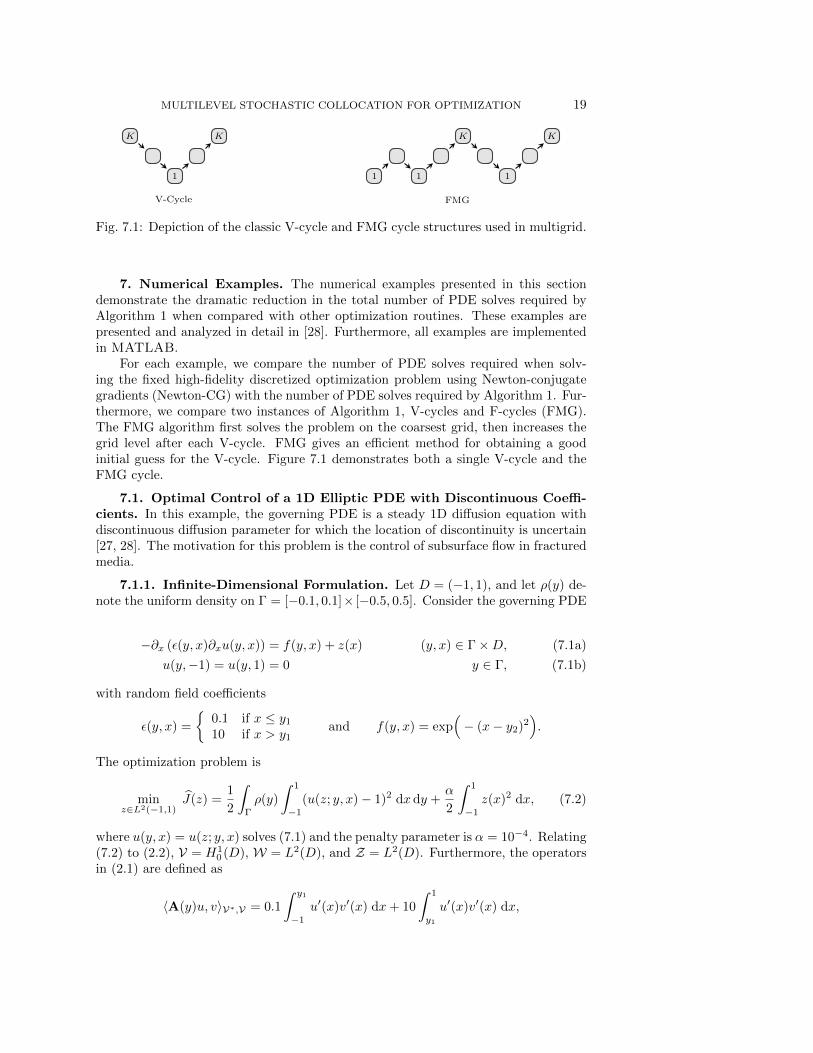
7. Numerical Examples. The numerical examples presented in this sectiondemonstrate the dramatic reduction in the total number of PDE solves required byAlgorithm 1 when compared with other optimization routines. These examples arepresented and analyzed in detail in [28]. Furthermore, all examples are implementedin MATLAB.

For each example, we compare the number of PDE solves required when solv-ing the fixed high-fidelity discretized optimization problem using Newton-conjugategradients (Newton-CG) with the number of PDE solves required by Algorithm 1. Fur-thermore, we compare two instances of Algorithm 1, V-cycles and F-cycles (FMG).The FMG algorithm first solves the problem on the coarsest grid, then increases thegrid level after each V-cycle. FMG gives an efficient method for obtaining a goodinitial guess for the V-cycle. Figure 7.1 demonstrates both a single V-cycle and theFMG cycle.

7.1. Optimal Control of a 1D Elliptic PDE with Discontinuous Coeffi-cients. In this example, the governing PDE is a steady 1D diffusion equation withdiscontinuous diffusion parameter for which the location of discontinuity is uncertain[27, 28]. The motivation for this problem is the control of subsurface flow in fracturedmedia.

7.1.1. Infinite-Dimensional Formulation. Let D = (−1, 1), and let ρ(y) de-note the uniform density on Γ = [−0.1, 0.1]× [−0.5, 0.5]. Consider the governing PDE

−∂x (ε(y, x)∂xu(y, x)) = f(y, x) + z(x) (y, x) ∈ Γ×D, (7.1a)

u(y,−1) = u(y, 1) = 0 y ∈ Γ, (7.1b)

with random field coefficients

ε(y, x) =

{0.1 if x ≤ y1

10 if x > y1and f(y, x) = exp

(− (x− y2)2

).

The optimization problem is

minz∈L2(−1,1)

J(z) =1

2

∫Γ

ρ(y)

∫ 1

−1

(u(z; y, x)− 1)2 dx dy +α

2

∫ 1

−1

z(x)2 dx, (7.2)

where u(y, x) = u(z; y, x) solves (7.1) and the penalty parameter is α = 10−4. Relating(7.2) to (2.2), V = H1

0 (D), W = L2(D), and Z = L2(D). Furthermore, the operatorsin (2.1) are defined as

〈A(y)u, v〉V∗,V = 0.1

∫ y1

−1

u′(x)v′(x) dx+ 10

∫ 1

y1

u′(x)v′(x) dx,

20 D. P. KOURI

N(u, y) ≡ 0, and F(z, y) = b(y)−B(y)z, where

〈b(y), v〉V∗,V =

∫ 1

−1

f(y, x)v(x) dx and 〈B(y)z, v〉V∗,V = −∫ 1

−1

z(x)v(x) dx.

Additionally, C is the canonical injection from H10 (D) into L2(D) and w ≡ 1. The

solution to (7.1) is continuous with respect to y ∈ Γ but need not be differentiable. Tocircumvent this complication, we use the domain decomposition formulation describedin [28].

7.1.2. Discretization. We discretize the PDE (7.1) in D using piecewise linearfinite elements. The finite-element mesh varies for each collocation point and is uni-form on each subinterval [−1, y1] and [y1, 1]. The control variable is also discretizedby using continuous piecewise linear finite elements on a uniform mesh of N = 128 in-tervals. Furthermore, we construct the sparse-grid hierarchy using isotropic Smolyaksparse grids built on 1D Gauss-Patterson points with maximum level fixed to K = 8.The largest sparse grid has Q8 = 1, 793 points.

7.1.3. Spectral Analysis of the Discretized Hessians. Since J(z) is quadratic,the estimates derived in Section 6 apply when CG is used as smoothers in Algo-rithm 1. After discretization, the Hessian matrix at each sparse-grid level is boundedand positive-definite. The maximum and minimum eigenvalues of the Hessian matri-ces are relatively constant between levels. At each level, the maximum eigenvalue isapproximately 1.64 × 10−2, and the minimum is approximately 3.85 × 10−7. Sincethe Hessians are positive definite, Theorem 6.1 and the work bounds derived in Sec-tion 6 apply. The V-cycle error bound in Theorem 6.1 depends on the generalizedeigenvalues of the matrix pencils (∇2Jk(z),∇2Jk−1(z)). The maximum and minimumgeneralized eigenvalues for each level for this hierarchy of matrix pencils are approxi-mately one, as proven in Section 6. Figure 7.2 depicts the absolute difference betweenone and the maximum (solid red) and minimum (solid black) generalized eigenvalues.As expected from the analysis in Section 6, the decay of the errors is approximatelylinear with respect to log10Qk. The red dashed line was fit by using the maximumeigenvalues and decays at a rate of ν = 1.63. The black dashed line was fit by usingthe minimum eigenvalues and decays at a rate of ν = 2.08.

7.1.4. Optimization Results. We solve the high fidelity problem (K = 8)using CG, which we terminate according to the relative residual stopping criterion

‖∇2JK(z)s+∇JK(z)‖Z ≤ 10−6‖∇JK(z)‖Z . (7.3)

The multilevel collocation algorithm uses CG as pre- and post-smoothers at eachlevel. Algorithm 1 also uses CG to solve (4.1) on the coarsest grid (k = 1) using therelative residual condition (7.3). The smoothers are computed as in Theorem 6.4 withT1,k = K−k+1 = T2,k iterations of CG at each level. The smoother exits early if therelative residual condition (7.3) is satisfied. Disregarding early exit of the smoothersresults in the theoretical upper bound on the number of PDE solves for one V-cycle

WK . 28QK + 2(N1CG + 1) = 50,280 PDE solves,

where the total number of CG iterations on the coarse grid was N1CG = 37.

The results for this example are tabulated in Table 7.1. Solving the high-fidelityoptimization problem with CG resulted in 100,408 PDE solves. For Algorithm 1, one


100

101

102

5

10

15

Qk

Eig

en

va

lue

s

100

101

102

10−5

10−4

10−3

10−2

10−1

100

101

102

Qk

Err

or

Fig. 7.2: Error between one and the minimum/maximum generalized eigenvalues

of the matrix pencil (∇2Jk(z),∇2Jk−1(z)). The horizontal axis is the number ofcollocation points. The error for the minimum (black lines) and maximum (red lines)eigenvalues decays linearly with respect to log10Qk. The decay rate is ν = 1.63 forthe minimum eigenvalues and ν = 2.08 for the maximum eigenvalues.

JK(z) PDE Solves Ratio Theoretical RatioCG 0.12638509 100,408 1.00 - -iCG 0.12638509 67,880 1.48 - -V-Cycle(1) 0.12638715 20,586 4.88 50,280 2.00V-Cycle(2) 0.12638510 37,758 2.66 100,560 1.00FMG 0.12638509 18,114 5.54 - -

Table 7.1: Final objective value, number of PDE solves, ratio of PDE solves com-pared with CG, and theoretical upper bound on the number of PDE solves for eachalgorithm: CG for the high-fidelity problem (CG), inexact CG (iCG), one and twoV-cycles (V-Cycle(i), i=1,2), and one F-cycle of Algorithm 1 (FMG).

V-cycle required 36, 760 PDE solves and reduced the norm of the gradient on thefinest level K = 8 to approximately 10−5. Two V-cycles required 64,940 PDE solvesand satisfied the relative residual condition (7.3). FMG required 24,558 PDE solvesand also satisfied the relative residual condition (7.3). All instances of Algorithm 1resulted in a reduction in PDE solves when compared with CG on the fixed high-fidelity grid, but FMG was the clear winner with a savings of over 4 times fewer PDEsolves.

7.2. Optimal Control of Steady Burger’s Equation. We now consider theoptimal control of the steady Burger’s equation. Optimal control of the deterministicBurger’s equation is analyzed in [46].

22 D. P. KOURI

7.2.1. Infinite-Dimensional Formulation. Let D = (0, 1), and let ρ(y) de-note the uniform density on Γ = [−1, 1]4. Consider the governing PDE

−ν(y)∂xxu(y, x) + u(y, x)∂xu(y, x) = f(y, x) + z(x) (y, x) ∈ Γ×D, (7.4a)

u(y, 0) = d0(y), u(y, 1) = d1(y) y ∈ Γ, (7.4b)

where the random field coefficients are

ν(y) = 10y1−2, f(y, x) =y2

100, d0(y) = 1 +

y3

1000, and d1(y) =

y4

1000.

The optimization problem is

minz∈L2(−1,1)

J(z) =1

2

∫Γ

ρ(y)

∫ 1

−1

(u(z; y, x)− 1)2 dx dy +α

2

∫ 1

−1

z(x)2 dx, (7.5)

where u(y, x) = u(z; y, x) solves (7.4) and the penalty parameter is α = 10−3. Relating(7.5) to (2.2), the function spaces are V = H1

0 (D), W = L2(D), and Z = L2(D). Foreach y ∈ Γ, the control operator, F(·, y) : Z → V∗, can be written as

F(z, y) = −b(y)−Bz.

The operators A : Γ → L(V,V∗), B : Γ → L(Z,V∗), N : V → V∗ and b : Γ → V∗are defined in [28]. Moreover, the observation operator C is the canonical injection ofH1

0 (D) into L2(D) and w ≡ 1.

7.2.2. Discretization. We discretize the state and control variables using con-tinuous piecewise linear finite elements on a uniform partition of D = (0, 1). Tosufficiently resolve the possible stiff behavior of (7.4), we use a mesh of N = 512uniform intervals. To solve the resulting system of finite-dimensional nonlinear equa-tions, we use Newton’s method with a backtracking line search. Furthermore, weconstruct the sparse-grid hierarchy using isotropic Smolyak sparse grids built on 1DClenshaw-Curtis points with maximum level fixed to K = 8. The largest sparse gridhas Q8 = 7, 537 points.

7.2.3. Optimization Results. We solve the high-fidelity optimization problem(K = 8) and the coarse-grid problem (4.1) using Newton-CG. We terminate CG usingthe relative residual stopping condition,

‖∇2Jk(z)s+∇Jk(z)‖Z ≤ ηk(z)‖∇Jk(z)‖Z , (7.6)

where the forcing function, ηk : Z → (0, 1), is defined as

ηk(z) = min{10−2, ‖∇Jk(z)‖Z}. (7.7)

This choice of ηk ensures q-quadratic convergence of Newton-CG whenever the initialguess z0 ∈ Z is sufficiently close to the optimal solution z∗ ∈ Z [38, Thm. 7.2]. Toglobalize Newton-CG, we employ a backtracking line search. Furthermore, we exitNewton-CG if the norm of the gradient of the objective function is less than thegradient tolerance gtol. For the high-fidelity problem gtol = 10−6 whereas for thecoarse-grid problem gtol = 10−8.

Similarly, we use a finite number of iterations of inexact Newton with inexactCG (Newton-iCG) for pre- and post-smoothing. We require inexact CG because weuse Algorithm 2 for Hessian-times-vector computations. To apply the smoothers, we


Nonlinear Ratio Linear RatioNewton-CG 30,148 1.00 678,330 1.00Newton-iCG 30,148 1.00 45,556 14.89V-Cycle(1) 34,198 0.88 37,708 17.99FMG 12,473 2.42 14,903 45.52

Table 7.2: Number of nonlinear and linear PDE solves required by the four differentalgorithms: Newton-CG with a backtracking line search, Newton with inexact CG andbacktracking line search (Newton-iCG), one V-cycle of Algorithm 1 (V-Cycle(1)), andone F-cycle of Algorithm 1 (FMG). “Ratio” refers to the ratio of the number of solvesfor Newton-CG with the number of solves for the other algorithms.

perform T1,k = T2,k = 1 outer iterations of Newton-iCG. That is, we apply inexactCG to approximately solve the Newton system (6.2) at each level, k. Inexact CG isterminated according to the relative residual condition (7.6) where, for fixed z ∈ Z,the forcing function is set to

ηk(z) = min{2−(K−k+1), ‖∇Jk(z)‖1/2Z }

for each level k. This specific choice of ηk ensures q-superlinear convergence ofNewton-CG [38, Thm. 7.2] and permits less work on the finer grids.

The primary computational work for general nonlinear PDE constrained opti-mization problems is PDE solves. To evaluate the objective function, we must solveQk deterministic instances of the state equation (7.4). To compute the gradient, werequire Qk nonlinear and Qk linear PDE solves corresponding to the state and adjointequations, respectively. To apply the Hessian to a vector, we require the solution tothe state equation, the adjoint equation, and the state and adjoint sensitivity equa-tions which, is a total of Qk nonlinear PDE solves and 3Qk linear PDE solves. Thetotal number of PDE solves can be reduced by storing state and adjoint variables,although recomputation may be essential depending on memory limitations. We storestate and adjoint variables in our implementation.

As in the previous example, we compare the cost of the high-fidelity solution withNewton-iCG, one V-cycle of Algorithm 1, and one F-cycle of Algorithm 1 (FMG). Forthe high-fidelity problem, Newton-CG required 30, 148 nonlinear and 678, 330 linearPDE solves to meet the gradient tolerance. By using inexact CG to solve the Newtonsystem, we reduce the number of linear PDE solves to 45, 556 while maintaining thenumber of nonlinear solves. After one V-cycle, Algorithm 1 successfully met thegradient tolerance. Although this V-cycle required more nonlinear PDE solves, itreduced the number of linear PDE solves by a factor of 17.99 when compared withNewton-CG. On the other hand, FMG successfully met the gradient tolerance andonly required 27, 376 nonlinear and linear PDE solves, 14, 903 of which were nonlinearPDE solves. FMG reduced the total number of nonlinear PDE solves by a factor of2.42 and linear PDE solves by a factor of 45.52 when compared with Newton-CG.These results are tabulated in Table 7.2.

8. Conclusions. In this work, we present a hierarchical sparse-grid discretiza-tion for optimization problems governed by PDEs with uncertain coefficients, andwe apply the MG/OPT framework [33, 30] to exploit this multilevel-in-sample-spacediscretization. The MG/OPT algorithm, Algorithm 1, is provably first-order con-

24 D. P. KOURI

vergent under standard assumptions. The hierarchical sparse-grid discretized opti-mization problems can similarly be handled with other globally convergent variantsof MG/OPT such as recursive trust-regions [21, 22, 23, 24] and the multilevel line-search approach [47].

In the case of quadratic optimal control of linear PDEs, we derived explicit upperbounds on the number of PDE solves required for a single V-cycle of Algorithm 1. Wealso proved error bounds for one V-cycle when CG is used as a pre- and post-smoother.We present numerical examples that confirm these upper bounds, and we demonstratethe immense reduction in the number of PDE solves required by Algorithm 1 whencompared with Newton-CG applied to a fixed high-fidelity discretized problem.

The number of PDE solves can further be reduced by using the adaptive collo-cation approach in [27, 28] as a pre- and post-smoother. Alternatively, with slightmodification, one can apply the MG/OPT algorithm to solve the trust-region sub-problems that arise in the adaptive collocation framework of [27, 28] The frameworkin [27, 28] adaptively builds a hierarchy of sparse-grid index sets that can be used inthe multilevel framework presented here. This coupling of the multilevel and adaptiveapproach is ideal as both methods perform a majority of their work on coarse sparsegrids, resulting in significantly fewer PDE solves. In addition, the adaptive approachexploits any anisotropic features of the sample space to further reduce the number ofcollocation points. This coupling is left as future work.

REFERENCES

[1] I. Babuska, F. Nobile, and R. Tempone, A stochastic collocation method for elliptic partialdifferential equations with random input data, SIAM Rev., 52 (2010), pp. 317–355.

[2] I. Babuska, R. Tempone, and G. E. Zouraris, Galerkin finite element approximations ofstochastic elliptic partial differential equations, SIAM J. Numer. Anal., 42 (2004), pp. 800–825 (electronic).

[3] , Solving elliptic boundary value problems with uncertain coefficients by the finite elementmethod: the stochastic formulation, Comput. Methods Appl. Mech. Engrg., 194 (2005),pp. 1251–1294.

[4] V. Barthelmann, E. Novak, and K. Ritter, High dimensional polynomial interpolationon sparse grids, Adv. Comput. Math., 12 (2000), pp. 273–288. Multivariate polynomialinterpolation.

[5] F. Bastin, C. Cirillo, and Ph. L. Toint, An adaptive Monte Carlo algorithm for computingmixed logit estimators, Comput. Manag. Sci., 3 (2006), pp. 55–79.

[6] A. Borzı, Multilevel methods in optimization with partial differential equations. Lecture notes,Institut fur Mathematik und Wissenschaftliches Rechnen, Karl-Franzens-Universitat Graz,Graz, Austria.

[7] A. Borzı, Multigrid methods for optimality systems, tech. report, Institut fur Mathematik undWissenschaftliches Rechnen, Karl-Franzens Universtiat Graz, 2003. Habilitationsschrift.

[8] , Multigrid methods for parabolic distributed optimal control problems, J. Comput. Appl.Math., 157 (2003), pp. 365–382.

[9] A. Borzı, On the convergence of the MG/OPT method, Proc. Appl. Math. Mech., 5 (2005),pp. 735-736.

[10] A. Borzı and G. Borzı, An efficient algebraic multigrid method for solving optimality systems,Comput. Vis. Sci., 7 (2004), pp. 183–188.

[11] A. Borzi, K. Ito, and K. Kunisch, Optimal control formulation for determining optical flow,SIAM J. Sci. Comput., 24 (2002), pp. 818–847 (electronic).

[12] A. Borzı and V. Schulz, Multigrid methods for PDE optimization, SIAM Review, 51 (2009),pp. 361–395.

[13] , Computational Optimization of Systems Governed by Partial Differential Equations,Computational Science and Engineering, Vol. 8, SIAM, Philadelphia, 2012.

[14] A. Borzı, V. Schulz, C. Schillings, and G. von Winckel, On the treatment of distributeduncertainties in PDE constrained optimization, GAMM Mitteilungen, 33 (2010), pp. 230–246.


[15] A. Borzı and G. von Winckel, Multigrid methods and sparse-grid collocation techniques forparabolic optimal control problems with random coefficients, SIAM J. Sci. Comput., 31(2009), pp. 2172–2192.

[16] R. H. Byrd, G. M. Chin, W. Neveitt, and J. Nocedal, On the use of stochastic hessianinformation in optimization methods for machine learning, SIAM Journal on Optimization,21 (2011), pp. 977–995.

[17] B. J. Debusschere, H. N. Najm, P. P. Pebay, O. M. Knio, R. G. Ghanem, and O. P. LeMaıtre, Numerical challenges in the use of polynomial chaos representations for stochasticprocesses, SIAM J. Sci. Comput., 26 (2004), pp. 698–719 (electronic).

[18] X. Du, E. Haber, M. Karampataki, and D. B. Szyld, Varying iteration accuracty usinginexact conjugate gradients in control problems governed by pdes, Tech. Report 08-06-27,Department of Mathematics, Temple University, 2008.

[19] T. Gerstner and M. Griebel, Numerical integration using sparse grids, Numer. Algorithms,18 (1998), pp. 209–232.

[20] , Dimension-adaptive tensor-product quadrature, Computing, 71 (2003), pp. 65–87.[21] S. Gratton, A. Sartenaer, and Ph. L. Toint, On recursive multiscale trust-region algo-

rithms for unconstrained minimization, in Oberwolfach Reports: Optimization and Appli-cations, C. Lemarechal F. Jarre and J. Zowe, eds., 2005.

[22] , Second-order convergence properties of trust-region methods using incomplete curvatureinformation, with an application to multigrid optimization, J. Comput. Math., 24 (2006),pp. 676–692.

[23] , Recursive trust-region methods for multiscale nonlinear optimization, SIAM J. Optim.,19 (2008), pp. 414–444.

[24] C. Groß and R. Krause, On the convergence of recursive trust-region methods for multiscalenon-linear optimization and applications to non-linear mechanics, SIAM J. Numer. Anal.,47 (2009), pp. 3004–3069.

[25] W. Hackbusch, Multigrid Methods and Applications, Computational Mathematics, Vol. 4,Springer–Verlag, Berlin, 1985.

[26] D. P. Kouri, Optimization governed by stochastic partial differential equations, master’s thesis,Department of Computational and Applied Mathematics, Rice University, Houston, TX,2010. Available as CAAM TR10-20.

[27] , An Approach for the Adaptive Solution of Optimization Problems Governed by PartialDifferential Equations with Uncertain Coefficients, PhD thesis, Department of Computa-tional and Applied Mathematics, Rice University, Houston, TX, May 2012. Available asCAAM TR12-10.

[28] D. P. Kouri, M. Heinkenschloss, D. Ridzal, and B. G. van Bloemen Waanders, A trust-region algorithm with adaptive stochastic collocation for pde optimization under uncer-tainty, Tech. Report ANL/MCS-P3035-0912, Department of Mathematics and ComputerScience, Argonne National Laboratory, 2012.

[29] R. M. Lewis and S. G. Nash, A multigrid approach for the optimization of systems governedby differential equations, tech. report, American INstitute of Aeronautics and Astronautics,2000.

[30] , Model problems for the multigrid optimization of systems governed by differential equa-tions, SIAM J. Sci. Comput., 26 (2005), pp. 1811–1837 (electronic).

[31] J. S. Liu, Monte Carlo strategies in scientific computing, Springer Series in Statistics, Springer,New York, 2008.

[32] M. Motamed, F. Nobile, and R. Tempone, A stochastic collocation method for the second or-der wave equation with a discontinuous random speed, Tech. Report MOX Report 36/2011,MOX Modeling and Scientific Computing, Politecnico di Milano, Italy, 2011.

[33] S. G. Nash, A multigrid approach to discretized optimization problems, Optim. Methods Softw.,14 (2000), pp. 99–116. International Conference on Nonlinear Programming and VariationalInequalities (Hong Kong, 1998).

[34] , Convergence and descent properties for a class of multilevel optimization algorithms,tech. report, Systems Engineering and Operators Research Deptartment, George MasonUniversity, 2010.

[35] F. Nobile and R. Tempone, Analysis and implementation issues for the numerical approx-imation of parabolic equations with random coefficients, Int. J. Numer. Methods Engrg.,80 (2009), pp. 979–1006.

[36] F. Nobile, R. Tempone, and C. G. Webster, An anisotropic sparse grid stochastic collocationmethod for partial differential equations with random input data, SIAM J. Numer. Anal.,46 (2008), pp. 2411–2442.

[37] , A sparse grid stochastic collocation method for partial differential equations with ran-

26 D. P. KOURI

dom input data, SIAM Journal on Numerical Analysis, 46 (2008), pp. 2309–2345.[38] J. Nocedal and S. J. Wright, Numerical Optimization, second ed., Springer Verlag, Berlin,

2006.[39] W.M. Patterson, Iterative methods for the solution of a linear operator equation in Hilbert

space - a survey, Lecture Notes in Mathematics, Springer-Verlag, 1974.[40] Y. Saad, Iterative Methods for Sparse Linear Systems, PWS Publishing Company, Boston,

1996.[41] V. Simoncini and D. B. Szyld, Flexible inner-outer Krylov subspace methods, SIAM J. Numer.

Anal., 40 (2002), pp. 2219–2239 (electronic) (2003).[42] S. A. Smoljak, Quadrature and interpolation formulae on tensor products of certain function

classes, Soviet Math. Dokl., 4 (1963), pp. 240–243.[43] U. Trottenberg, C. W. Oosterlee, and A. Schuller, Multigrid, Academic Press, San

Diego, CA, 2001. With contributions by A. Brandt, P. Oswald and K. Stuben.[44] M. Vallejos and A. Borzı, Multigrid optimization methods for linear and bilinear elliptic

optimal control problems, Computing, 82 (2008), pp. 31–52.[45] J. van den Eshof and G. L. G. Sleijpen, Inexact Krylov subspace methods for linear systems,

SIAM J. Matrix Anal. Appl., 26 (2004), pp. 125–153 (electronic).[46] S. Volkwein, Mesh–independence for an augmented Lagrangian–SQP method in Hilbert space,

SIAM J. Control and Optimization, 38 (2000), pp. 767–785.[47] Z. Wen and D. Goldfarb, A line search multigrid method for large-scale nonlinear optimiza-

tion, SIAM J. Optim., 20 (2009), pp. 1478–1503.[48] D. Xiu and J. S. Hesthaven, High-order collocation methods for differential equations with

random inputs, SIAM J. Sci. Comput., 27 (2005), pp. 1118–1139 (electronic).[49] D. Xiu and G. E. Karniadakis, Modeling uncertainty in flow simulations via generalized

polynomial chaos, J. Comput. Phys., 187 (2003), pp. 137–167.

The submitted manuscript has been created by UChicago Argonne, LLC, Operatorof Argonne National Laboratory (“Argonne”). Argonne, a U.S. Department ofEnergy Office of Science laboratory, is operated under Contract No. DE-AC02-06CH11357. The U.S. Government retains for itself, and others acting on its behalf,a paid-up nonexclusive, irrevocable worldwide license in said article to reproduce,prepare derivative works, distribute copies to the public, and perform publicly anddisplay publicly, by or on behalf of the Government.

a multilevel stochastic collocation … is a template for the application of multigrid to...

Documents