95 of 119

Properties of the Grid TransferOperators: Interpolation

• Interpolation: or

: ℜ N/2-1 ℜ N-1

• For N=8,

• has full rank and null space .

I2hh

I 22

hhhh Ω→Ω:

I2hh =

1211

211

21

21

I2hh φ

96 of 119

Spectral properties of .

• How does act on the eigenvectors of ?

• Consider , 1 ≤ k ≤ N/2-1, 0 ≤ j ≤ N/2

• Good Exercise: show that the modes of areNOT preserved by , but that the space ispreserved:

I2hh

I2hh A 2h

/

π

=)(Nkj

wj

hk2

2nis

A 2h

I2hh W k

wN

kw

Nk

wI 2222

hk

hk

hk

hh

π

−

π

=2

nis2

soc ′

−= wswc hkk

hkk ′

97 of 119

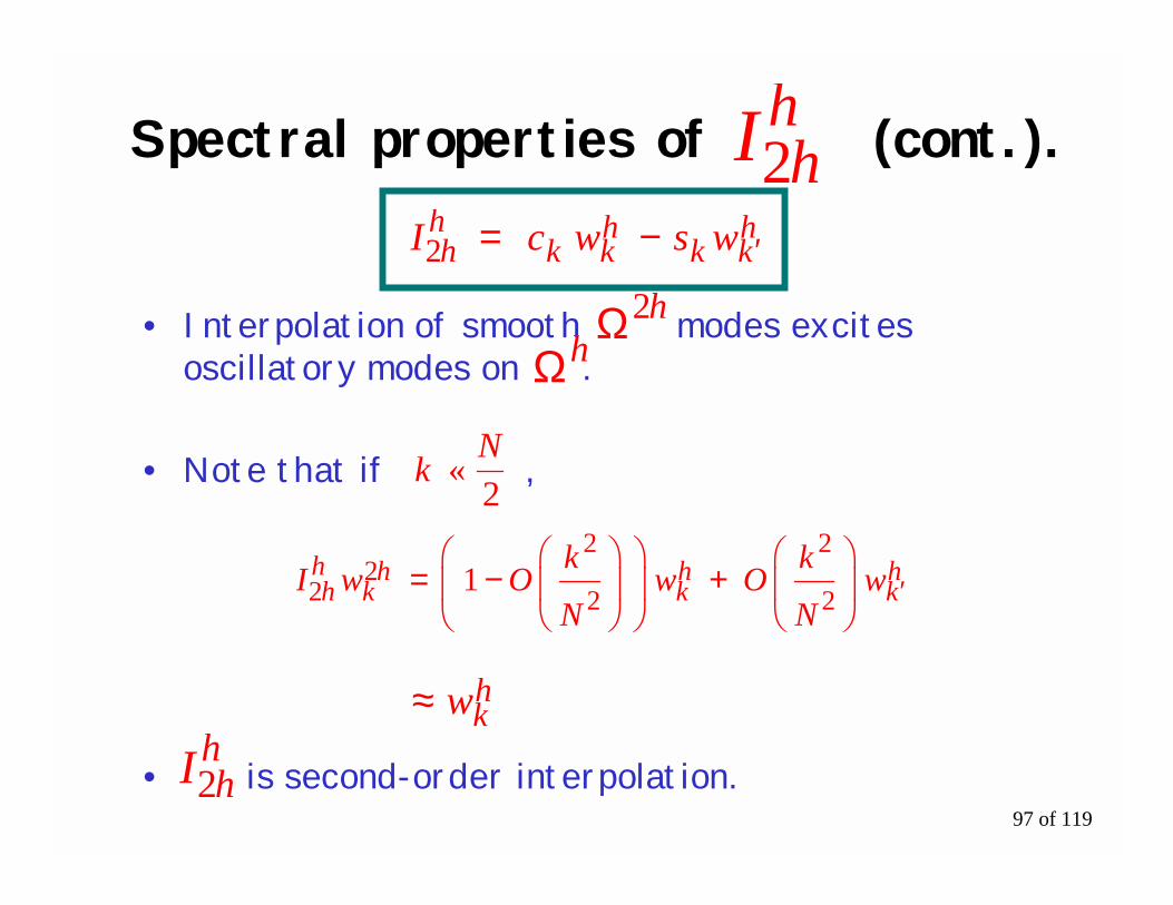
Spectral properties of (cont.).

• Interpolation of smooth modes excitesoscillatory modes on .

• Note that if ,

• is second-order interpolation.

I2hh

wswcI2hkk

hkk

hh −= ′

Ω2h

Ωh

Nk

2«

wN

kOw

N

kOwI

2

2

2

22

2hk

hk

hk

hh

+

−

= 1 ′

≈ whk

I2hh

98 of 119

The Range of .

• The range of is the span of the columns of

• Let be the ith column of .

• All the Fourier modes of are needed torepresent Range( )

I2hh

I2hh I2

hh

ξi I2hh

:ξi

I2hh

≠,=ξ khkk

N

k

hi

−

=

1

1bwb 0

A h

99 of 119

Use all the facts to analyze thecoarse-grid correction scheme1) Relax times on :

2) Compute and restrict residual

3) Solve residual equation

4) Correct fine-grid solution .

• The entire process appears as

• The exact solution satisfies

Ωh vRv hh ← α1

vAfIf 22 hhhhh

h )−(←

fAv 2122 hhh )(=−

vIvv hhh

hh +← 22

vRAfIAIvRv hhhhh

hhh

hh )−()(+← α−α 2122

uRAfIAIuRu hhhhh

hhh

hh )−()(+← α−α 2122

α

100 of 119

Error propagation of the coarse-grid correction scheme

• Subtracting the previous two expressions, we get

• How does CG act on the modes of ? Assumeconsists of the modes and forand .

• We know how act on and .

eRAIAIIe hhhh

hhh

h )(−← 2122

α−

eGCe hh←

A h

whk′wh

k 21 /≤≤ NkkNk −=′

IAIAR−α ,)(,,, h

hhh

hh

2122

whk wh

k′

101 of 119

Error propagation of CG• For now, assume no relaxation . Then

is invariant under CG.

where

=α 0wwW h

khkk ,= naps ′

wswswGC hkk

hkk

hk += ′

wcwcwGC hkk

hkk

hk ′′ +=

Nk

ck

π

=2

soc 2N

ksk

π

=2

nis 2

102 of 119

CG error propagation for k << N

• Consider the case k << N (extremely smooth andoscillatory modes):

• Hence, CG eliminates the smooth modes but doesnot damp the oscillatory modes of the error!

wN

kOw

N

kOw kkk

+

→2

2

2

2

′

wN

kOw

N

kOw kkk

−

+

−

→ 112

2

2

2

′

103 of 119

Now consider CG with relaxation

• Next, include relaxation sweeps. Assume thatthe relaxation preserves the modes of(although this is often unnecessary). Letdenote the eigenvalue of associated with .For k < < N/2,

αR A h

λkR wk

wswsw kkkkkkk λ+λ→ ′αα

wcwcw kkkkkkk ′α′

α′′ λ+λ→

Small!

Small!

104 of 119

The crucial observation:

• Between relaxation and the coarse-grid correction, both smooth andoscillatory components of the errorare effectively damped.

• This is essentially the “spectral”picture of how multigrid works. Weexamine now another viewpoint, the“algebraic” picture of multigrid.

105 of 119

Recall the variational properties

• All the analysis that follows assumes that thevariational properties hold:

IAIA 222 h

hhh

hh =

IcI 22

Thh

hh )(=

(Galerkin Condition )

for c in ℜ

106 of 119

Algebraic interpretation ofcoarse-grid correction

• Consider the subspaces that make up andΩh Ω2h

IR )( 2hh IN )( h

h2Ωh

Ω2h IR )( hh2

I2hh I h

h2

For the rest of this talk, ‘R( )’refers to the Range of a linearoperator.

From the fundamental theoremof linear algebra:

orIRIN ))((⊥)( Thh

hh

22

IRIN )(⊥)( hh

hh 22

107 of 119

Subspace decomposition of .• Since has full rank, we can say, equivalently,

( where means that ).

• Therefore, any can be written as where and .

• Hence,

Ωh

A h

AINIR )(⊥)( 22

hhhA

hh h

yx ⊥A h yxA h =, 0

eh tse hhh +=IRs h

hh )(∈ 2 AINt hh

hh )(∈ 2

)(⊕)(=Ω hhh

hh

h AINIR 22

108 of 119

Characteristics of the subspaces

• Since for some , weassociate with the smooth components of .But, generally has all Fourier modes in it (recallthe basis vectors for ).

• Similarly, we associate with oscillatorycomponents of , although generally has allFourier modes in it as well. Recall that isspanned by therefore isspanned by the unit vectorsfor odd i, which “look” oscillatory.

qIs hhh

h = 22 q 22 hh Ω∈

sh eh

shI2

hh

t h

eh t h

IN )( hh2

=η ih

i eA AIN )( hhh2

e Thi ),...,,,,...,,(= 001000

109 of 119

qIAIAIIsGC hhh

hhh

hhh

h )(−= 22

2122

−

Algebraic analysis of coarse-gridcorrection

• Recall that (without relaxation)

• First note that if then .This follows since for someand therefore

• It follows that , that is, the nullspace of coarse-grid correction is the range ofinterpolation.

AIAIIGC )(−= 2122

hhh

hhh

−

IRs hh

h )(∈ 2 sGC h = 0qIs hh

hh = 2

2 q 22 hh Ω∈

= 0

IRGCN )(=)( 2hh

A 2h by Galerkin property

110 of 119

More algebraic analysis ofcoarse-grid correction

• Next, note that if then

• Therefore .

• CG is the identity on

AINt hhh

h )(∈ 2

tAIAIItGC hhhh

hhh

h )(−= 2122

−

ttGC hh =0

AIN )( hhh2

111 of 119

How does the algebraic picturefit with the spectral view?

• We may view in two ways:

=

that is,

or as

Ωh

Low frequency modes1 ≤ k ≤ N/2

High frequency modesN/2 < k < N Ωh ⊕

⊕=Ωh HL

)(⊕)(=Ω hhh

hh

h AINIR 22

112 of 119

Actually, each view is just partof the picture

• The operations we have examined work ondifferent spaces!

• While is mostly oscillatory, it isn’t .and while is mostly smooth, it isn’t .

• Relaxation eliminates error from .

• Coarse-grid correction eliminates error from

H

H

IR )( 2hh L

AIN )( hhh2

IR )( 2hh

113 of 119

How it actually works (cartoon)

IR )( 2hh

AIN )( hhh2

eh

sh

t h

H

L

114 of 119

Relaxation eliminates H, butincreases the error in .

IR )( 2hh

AIN )( hhh2

eh

sh

t h

H

L

IR )( 2hh

115 of 119

CG eliminates butincreases the error in H.

IR )( 2hh

AIN )( hhh2

eh

sh

t h

H

L

IR )( 2hh

116 of 119

Difficulties:anisotropic operators and grids

• Consider the operator :

• The same phenomenonoccurs for grids with muchlarger spacing in one directionthan the other:

),(=∂∂β−

∂∂

α−2

2

2

2yxf

yu

xu

-100 -50 0 50 1000

0.2

0.4

0.6

0.8

1

1.2 If then the GS-smoothingfactors in the x- and y-directions areshown at right.Note that GS relaxation does notdamp oscillatory components in the x-direction.

βα «

117 of 119

Difficulties: discontinuous oranisotropic coefficients

• Consider the operator :where

• Solutions: line-relaxation (where whole gridlinesof values are found simultaneously), and/or semi-coarsening (coarsening only in the strongly coupleddirection).

Again, GS-smoothing factors in the x- and y-directionscan be highly variable, and very often, GS relaxation doesnot damp oscillatory components in the one or bothdirections.

)∇),((•∇− uyxD

yxdyxd

yxdyxdyxD

),(),(

),(),(

=),(2212

2111

118 of 119

For nonlinear problems, use FAS (Full Approximation Scheme)

• Suppose we wish to solve: wherethe operator is non-linear. Then the linearresidual equation does not apply.

• Instead, we write the non-linear residual equation:

• This is transferred to the coarse grid as:

• We solve for and transfer theerror (only!) to the fine grid:

reA =

fuA =)(

ruAeuA =)(−)+(

uAfIeuA 2222 hhhhh

hhh ))(−(=)+(

euw 222 hhh +≡

uIwIuu hhh

hhh

hh )−(+← 222

119 of 119

Multigrid: increasingly, the righttool!

• Multigrid has been proven on a wide variety ofproblems, especially elliptic PDEs, but has also foundapplication among parabolic & hyperbolic PDEs,integral equations, evolution problems, geodesicproblems, etc.

• With the right setup, multigrid is frequently anoptimal (i.e., O(N)) solver.

• Multigrid is of great interest because it is one of thevery few scalable algorithms, and can be parallelizedreadily and efficiently!