a multi-phase supersonic jet impingement facility for thermal...

A MULTI-PHASE SUPERSONIC JET IMPINGEMENT FACILITY FOR THERMALMANAGEMENT

By

RICHARD RAPHAEL PARKER

A DISSERTATION PRESENTED TO THE GRADUATE SCHOOLOF THE UNIVERSITY OF FLORIDA IN PARTIAL FULFILLMENT

OF THE REQUIREMENTS FOR THE DEGREE OFDOCTOR OF PHILOSOPHY

UNIVERSITY OF FLORIDA

2012

c© 2012 Richard Raphael Parker

2

ACKNOWLEDGMENTS

Throughout my time in graduate school I have been helped by many people,

although I will try my best to include everyone, inevitably I will leave some people out.

For that I am sorry.

First and foremost I would like to thank my parents as without them this would not

be possible. Dad, you taught me what it meant to be a man, and I can’t express my

gratitude enough.

There have been a multitude of people in my lab that have helped me immensely,

Dr. Patrick Garrity, Dr. Ayyoub Mehdizadeh, Dr. Jameel Khan, and Dr. Fadi Alnaimat

(my current roommate) who have all graduated and are going places in the world, you

have provided help and motivation. Bradley Bon, Fotouh Al-Ragom (the lab mother), and

Cheng-Kang (Ken) Guan who are currently preparing for their dissertation defense, we

have all helped motive each other. Ben Greek, Prasanna Venvanalingam, Kyle Allen,

Like Li, and Nima Rahmatian, who are currently completing their degree requirements,

have helped me develop some of my presentation skills. I hope you have learned as

much from me as I have from you.

My friends in the Interdisciplinary Microsystems Group (IMG) who have provided

many opportunities to escape the pressures of graduate studies. I would specifically like

to thank my old roommate, Dr. Drew Wetzel, who let me bounce ideas off of him, Dr.

Matt Williams, who always ran the group football competitions and helped me reminisce

about my roots in South Carolina, and Brandon Bertolucci our official social chair. Thank

you all and good luck.

I would also like to thank my professors at the University of South Carolina. Dr.

Jamil Khan, whose heat transfer classes helped shape the foundation of my knowledge

in the thermal and fluid sciences, Dr. David Rocheleau who provided me with contacts

at the University of Florida, Dr. Phillip Voglewede who encouraged me to attend the

3

University of Florida, and finally Dr. Abdel Bayoumi, my undergraduate research advisor

who saw potential in me and provided many opportunities for me to grow.

Last, but not least, I would like to thank my committee. Dr. Orazem has helped

me learn things outside of my field and my comfort zone and for that I am grateful. Dr.

Hahn, your rigorous heat conduction class helped build the foundation for much of my

studies. Dr. Mei, you have helped me realize my potential for numerical studies and how

to know when a solution is good enough or when perfection is essential. Lastly I would

like to thank my chair, Dr. James F. Klausner. Dr. Klausner, you have kept me around,

even as I struggled, because you saw the potential in me. You’ve help keep some levity

in the lab with football talk and going to some excellent concerts. Most importantly,

you’ve helped me grow both professionally and as a person. For this you have my most

sincere gratitude.

4

TABLE OF CONTENTS

page

ACKNOWLEDGMENTS . . . . . . . . . . . . . . . . . . . . . . . . . . . . . . . . . . 3

LIST OF TABLES . . . . . . . . . . . . . . . . . . . . . . . . . . . . . . . . . . . . . . 8

LIST OF FIGURES . . . . . . . . . . . . . . . . . . . . . . . . . . . . . . . . . . . . . 9

NOMENCLATURE . . . . . . . . . . . . . . . . . . . . . . . . . . . . . . . . . . . . . 13

ABSTRACT . . . . . . . . . . . . . . . . . . . . . . . . . . . . . . . . . . . . . . . . . 17

CHAPTER

1 INTRODUCTION AND LITERATURE REVIEW . . . . . . . . . . . . . . . . . . 19

1.1 Literature Review . . . . . . . . . . . . . . . . . . . . . . . . . . . . . . . . 201.1.1 Single-Phase Jet Impingement . . . . . . . . . . . . . . . . . . . . 201.1.2 Mist and Spray Cooling . . . . . . . . . . . . . . . . . . . . . . . . 241.1.3 Supersonic Jet Impingement . . . . . . . . . . . . . . . . . . . . . 25

1.2 Summary . . . . . . . . . . . . . . . . . . . . . . . . . . . . . . . . . . . . 34

2 JET IMPINGEMENT FACILITY . . . . . . . . . . . . . . . . . . . . . . . . . . . 36

2.1 Impinging Jet Facility Systems . . . . . . . . . . . . . . . . . . . . . . . . 362.1.1 Air Storage System . . . . . . . . . . . . . . . . . . . . . . . . . . . 362.1.2 Water Storage and Flow Control System . . . . . . . . . . . . . . . 362.1.3 Air Pressure Control System . . . . . . . . . . . . . . . . . . . . . . 392.1.4 Air Mass Flow Measuring System . . . . . . . . . . . . . . . . . . . 392.1.5 Temperature and Pressure Measurements . . . . . . . . . . . . . . 422.1.6 Converging-Diverging Nozzle . . . . . . . . . . . . . . . . . . . . . 422.1.7 Data Acquisition System . . . . . . . . . . . . . . . . . . . . . . . . 43

2.2 Analysis of Impingement Facility . . . . . . . . . . . . . . . . . . . . . . . 442.2.1 Temperature and Pressure Upstream of the Nozzle . . . . . . . . . 442.2.2 Nozzle Exit Pressure Considerations . . . . . . . . . . . . . . . . . 462.2.3 Oblique Shock Waves at Nozzle Exit . . . . . . . . . . . . . . . . . 482.2.4 Complete Shock Structure of an Overexpanded Jet . . . . . . . . . 50

2.3 Summary . . . . . . . . . . . . . . . . . . . . . . . . . . . . . . . . . . . . 51

3 STEADY STATE EXPERIMENTS . . . . . . . . . . . . . . . . . . . . . . . . . . 53

3.1 Heater Construction . . . . . . . . . . . . . . . . . . . . . . . . . . . . . . 563.1.1 Physical Description . . . . . . . . . . . . . . . . . . . . . . . . . . 563.1.2 Theoretical Concerns . . . . . . . . . . . . . . . . . . . . . . . . . 57

3.2 Experimental Procedure . . . . . . . . . . . . . . . . . . . . . . . . . . . . 593.2.1 Two-Phase Experiments . . . . . . . . . . . . . . . . . . . . . . . . 593.2.2 Single-Phase Experiments . . . . . . . . . . . . . . . . . . . . . . . 62

5

3.3 Experimental Results . . . . . . . . . . . . . . . . . . . . . . . . . . . . . 633.3.1 Uncertainty Analysis . . . . . . . . . . . . . . . . . . . . . . . . . . 633.3.2 Single-Phase Results . . . . . . . . . . . . . . . . . . . . . . . . . 643.3.3 Two-Phase Results . . . . . . . . . . . . . . . . . . . . . . . . . . . 673.3.4 Evaporation Effects . . . . . . . . . . . . . . . . . . . . . . . . . . . 73

3.4 Comparison between Single and Two-Phase Jets . . . . . . . . . . . . . . 743.5 Discussion . . . . . . . . . . . . . . . . . . . . . . . . . . . . . . . . . . . 753.6 Summary . . . . . . . . . . . . . . . . . . . . . . . . . . . . . . . . . . . . 77

4 DETERMINATION OF HEAT TRANSFER COEFFICIENT USING AN INVERSEHEAT TRANSFER ANALYSIS . . . . . . . . . . . . . . . . . . . . . . . . . . . . 79

4.1 Inverse Problems . . . . . . . . . . . . . . . . . . . . . . . . . . . . . . . . 794.2 Introduction to Inverse Problem Solution Using the Conjugate Gradient

Method with Adjoint Problem . . . . . . . . . . . . . . . . . . . . . . . . . 814.2.1 The Direct Problem . . . . . . . . . . . . . . . . . . . . . . . . . . . 824.2.2 The Measurement Equation . . . . . . . . . . . . . . . . . . . . . . 824.2.3 The Indirect Problem . . . . . . . . . . . . . . . . . . . . . . . . . . 834.2.4 The Adjoint Problem . . . . . . . . . . . . . . . . . . . . . . . . . . 834.2.5 Gradient Equation . . . . . . . . . . . . . . . . . . . . . . . . . . . 854.2.6 Sensitivity Equation . . . . . . . . . . . . . . . . . . . . . . . . . . . 854.2.7 The Conjugate Gradient Method . . . . . . . . . . . . . . . . . . . 86

4.3 Factors Influencing Inverse Heat Transfer Problems . . . . . . . . . . . . . 884.3.1 Boundary Condition Formulation Effects . . . . . . . . . . . . . . . 884.3.2 Sensor Location Effects . . . . . . . . . . . . . . . . . . . . . . . . 914.3.3 Thermocouple Insertion Effects . . . . . . . . . . . . . . . . . . . . 92

4.4 Inverse Heat Transfer Problem Formulation . . . . . . . . . . . . . . . . . 954.4.1 Direct Problem . . . . . . . . . . . . . . . . . . . . . . . . . . . . . 964.4.2 Measurement Equation . . . . . . . . . . . . . . . . . . . . . . . . 974.4.3 Indirect Problem . . . . . . . . . . . . . . . . . . . . . . . . . . . . 984.4.4 Adjoint Problem . . . . . . . . . . . . . . . . . . . . . . . . . . . . . 984.4.5 Gradient Equation . . . . . . . . . . . . . . . . . . . . . . . . . . . 1014.4.6 Sensitivity Problem . . . . . . . . . . . . . . . . . . . . . . . . . . . 1014.4.7 Conjugate Gradient Method . . . . . . . . . . . . . . . . . . . . . . 1024.4.8 Stopping Criteria . . . . . . . . . . . . . . . . . . . . . . . . . . . . 1034.4.9 Algorithm . . . . . . . . . . . . . . . . . . . . . . . . . . . . . . . . 104

4.5 Numerical Method and Limitations . . . . . . . . . . . . . . . . . . . . . . 1054.5.1 Alternating Direction Implicit Method . . . . . . . . . . . . . . . . . 1054.5.2 Grid Stretching in the Z-Direction . . . . . . . . . . . . . . . . . . . 1064.5.3 Time step size complications . . . . . . . . . . . . . . . . . . . . . 108

4.6 Deconvolution for Thermocouple Impulse Response Functions . . . . . . 1084.6.1 Direct Problem . . . . . . . . . . . . . . . . . . . . . . . . . . . . . 1094.6.2 Indirect Problem . . . . . . . . . . . . . . . . . . . . . . . . . . . . 1104.6.3 Adjoint Problem . . . . . . . . . . . . . . . . . . . . . . . . . . . . . 1104.6.4 Gradient Equation . . . . . . . . . . . . . . . . . . . . . . . . . . . 110

6

4.6.5 Sensitivity Problem . . . . . . . . . . . . . . . . . . . . . . . . . . . 1104.6.6 Conjugate Gradient Method . . . . . . . . . . . . . . . . . . . . . . 1104.6.7 Stopping Criteria . . . . . . . . . . . . . . . . . . . . . . . . . . . . 1114.6.8 Algorithm . . . . . . . . . . . . . . . . . . . . . . . . . . . . . . . . 1114.6.9 Test Case . . . . . . . . . . . . . . . . . . . . . . . . . . . . . . . . 112

4.7 Summary . . . . . . . . . . . . . . . . . . . . . . . . . . . . . . . . . . . . 114

5 SENSOR DYNAMICS AND THE EFFECTIVENESS OF THE INVERSE HEATTRANSFER ALGORITHM . . . . . . . . . . . . . . . . . . . . . . . . . . . . . . 116

5.1 Thermocouple Measurement Dynamics . . . . . . . . . . . . . . . . . . . 1165.1.1 Low Biot Number Thermocouple Models . . . . . . . . . . . . . . . 1165.1.2 High Biot Number Thermocouple Models . . . . . . . . . . . . . . 1215.1.3 Design of Experiment . . . . . . . . . . . . . . . . . . . . . . . . . 1225.1.4 Experimental Results . . . . . . . . . . . . . . . . . . . . . . . . . . 1265.1.5 Comparison to Established Models . . . . . . . . . . . . . . . . . . 127

5.2 Inverse Heat Transfer Algorithm Verification . . . . . . . . . . . . . . . . . 1315.2.1 Inverse Quenching Parametric Study Setup . . . . . . . . . . . . . 1325.2.2 Error Assessment Methods . . . . . . . . . . . . . . . . . . . . . . 1365.2.3 Parametric Study Results . . . . . . . . . . . . . . . . . . . . . . . 1375.2.4 Heat Loss/Gain Effects . . . . . . . . . . . . . . . . . . . . . . . . . 1415.2.5 Effectiveness of the Inverse Heat Transfer Algorithm . . . . . . . . 142

5.3 Summary . . . . . . . . . . . . . . . . . . . . . . . . . . . . . . . . . . . . 144

6 CONCLUSIONS . . . . . . . . . . . . . . . . . . . . . . . . . . . . . . . . . . . 147

APPENDIX

A COMPLETE STEADY STATE TWO-PHASE HEAT TRANSFER JET RESULTS 151

B COMPLETE INVERSE HEAT TRANSFER ALGORITHM ERROR ASSESSMENTCONTOUR PLOTS . . . . . . . . . . . . . . . . . . . . . . . . . . . . . . . . . . 166

C IMAGES OF ORIFICES USED DURING EXPERIMENTS . . . . . . . . . . . . 172

REFERENCES . . . . . . . . . . . . . . . . . . . . . . . . . . . . . . . . . . . . . . . 175

BIOGRAPHICAL SKETCH . . . . . . . . . . . . . . . . . . . . . . . . . . . . . . . . 184

7

LIST OF TABLES

Table page

2-1 Water Mass Flowrate and Average Water Velocity for Different Regulator Pressuresand Orifice Sizes. . . . . . . . . . . . . . . . . . . . . . . . . . . . . . . . . . . 40

2-2 Area, temperature, and pressure ratios at various points in the jet impingementfacility. . . . . . . . . . . . . . . . . . . . . . . . . . . . . . . . . . . . . . . . . . 46

2-3 Nozzle exit pressure for various regulator pressures. . . . . . . . . . . . . . . . 47

3-1 Reynolds number and corresponding heat fluxes. . . . . . . . . . . . . . . . . . 62

5-1 Curve Fitting Constants for Rabin and Rittel’s thermocouple impulse responsemodel, from [114] . . . . . . . . . . . . . . . . . . . . . . . . . . . . . . . . . . . 121

5-2 RMS errors for L = 10 mm, and σDAQ = 0.2 C. . . . . . . . . . . . . . . . . . . 138

5-3 RMS errors for L = 10 mm, σDAQ = 1 C, and M = 8. . . . . . . . . . . . . . . . 139

5-4 RMS errors for L = 5 mm and σDAQ = 0.2 C. . . . . . . . . . . . . . . . . . . . 140

5-5 RMS error for L = 10 mm,σDAQ = 0.2 C, M = 8, and various values of σ forthe Biot number distribution. . . . . . . . . . . . . . . . . . . . . . . . . . . . . . 140

5-6 RMS error for L = 10 mm and M = 8 with different actual and simulated timeconstants. . . . . . . . . . . . . . . . . . . . . . . . . . . . . . . . . . . . . . . . 141

8

LIST OF FIGURES

Figure page

1-1 Solution of stagnation point flow . . . . . . . . . . . . . . . . . . . . . . . . . . 21

1-2 An illustration of the shock structure in the wall jet region. . . . . . . . . . . . . 26

1-3 Grease streak photograph. . . . . . . . . . . . . . . . . . . . . . . . . . . . . . 28

1-4 Numerical results of a flow field with a plate shock. . . . . . . . . . . . . . . . . 31

1-5 Jet centerline pressure fluctuations with and without moisture. . . . . . . . . . 32

1-6 Adiabatic and heated temperature variation with z/D. . . . . . . . . . . . . . . . 34

2-1 Illustration of the jet impingement facility. . . . . . . . . . . . . . . . . . . . . . . 37

2-2 Cross section of the mixing chamber. . . . . . . . . . . . . . . . . . . . . . . . 38

2-3 Thread details of the mixing chamber cross section. . . . . . . . . . . . . . . . 38

2-4 Orifice cross section. . . . . . . . . . . . . . . . . . . . . . . . . . . . . . . . . . 39

2-5 Theoretical vs measured mair . . . . . . . . . . . . . . . . . . . . . . . . . . . . . 41

2-6 Cross section of nozzle. . . . . . . . . . . . . . . . . . . . . . . . . . . . . . . . 43

2-7 Simplified view of the air flow path in the facility. . . . . . . . . . . . . . . . . . . 45

2-8 Illustration of the limiting cases for shock waves in the nozzle. . . . . . . . . . . 48

2-9 Illustration of an oblique shock wave at the nozzle exit. . . . . . . . . . . . . . . 49

2-10 Variation of flow properties downstream of an oblique shock wave. . . . . . . . 50

2-11 Structure of oblique shock waves. . . . . . . . . . . . . . . . . . . . . . . . . . 52

3-1 Stainless steel heater assembly. . . . . . . . . . . . . . . . . . . . . . . . . . . 54

3-2 Copper heater assembly. . . . . . . . . . . . . . . . . . . . . . . . . . . . . . . 55

3-3 Illustration of heater assembly used for steady state experiments. . . . . . . . . 57

3-4 Ice formation at adiabatic conditions. . . . . . . . . . . . . . . . . . . . . . . . . 60

3-5 Measured single-phase NuD spatial variation at different heat fluxes. . . . . . . 64

3-6 Spatial heater temperature variation at different applied heat fluxes. . . . . . . 65

3-7 Spatial variation of NuD at different ReD, a) unscaled and b) scaled. . . . . . . 66

3-8 Single-phase NuD at various nozzle height to diameter ratios. . . . . . . . . . . 67

9

3-9 Measured two-phase NuD spatial variation at different heat fluxes without iceformation. . . . . . . . . . . . . . . . . . . . . . . . . . . . . . . . . . . . . . . . 68

3-10 Measured two-phase NuD spatial variation at different heat fluxes with andwithout ice formation. . . . . . . . . . . . . . . . . . . . . . . . . . . . . . . . . 69

3-11 Spatial heater temperature variation, two-phase jet results. . . . . . . . . . . . 70

3-12 Two-phase NuD at various liquid mass fractions. . . . . . . . . . . . . . . . . . 71

3-13 Two-phase NuD number at various nozzle height to diameter ratios. . . . . . . 72

3-14 Heat transfer enhancement ratio at various liquid mass fractions. . . . . . . . . 74

3-15 Heat transfer enhancement ratio at various nozzle height to diameter ratios. . . 76

4-1 1-dimensional solid for the sensitivity problem. . . . . . . . . . . . . . . . . . . 89

4-2 Relative step sensivity coefficients at x∗ = 0.1 as a function of time. . . . . . . . 92

4-3 Relative step sensivity coefficient for a heat flux input. . . . . . . . . . . . . . . 93

4-4 Relative step sensivity coefficient for a temperature input. . . . . . . . . . . . . 93

4-5 Illustration of the heat transfer physics of the inverse problem formulation. . . . 96

4-6 Comparison of true temperature vs inverse results. . . . . . . . . . . . . . . . . 104

4-7 Effects of grid stretching. a) real domain and b) computational domain. . . . . 107

4-8 Time step results. . . . . . . . . . . . . . . . . . . . . . . . . . . . . . . . . . . 109

4-9 True and estimated impulse response function. . . . . . . . . . . . . . . . . . . 113

4-10 Convergence history. . . . . . . . . . . . . . . . . . . . . . . . . . . . . . . . . . 113

4-11 Output comparison. . . . . . . . . . . . . . . . . . . . . . . . . . . . . . . . . . 114

5-1 Illustration of the first order slab. . . . . . . . . . . . . . . . . . . . . . . . . . . 118

5-2 Illustration of the second order slab. . . . . . . . . . . . . . . . . . . . . . . . . 119

5-3 Example of a first and second order impulse response function. . . . . . . . . . 120

5-4 Impulse response functions using the model of Rabin and Rittel, adapted from[114]. . . . . . . . . . . . . . . . . . . . . . . . . . . . . . . . . . . . . . . . . . 122

5-5 Diagram of the copper disc assembly. . . . . . . . . . . . . . . . . . . . . . . . 123

5-6 Illustration of the experimental setup. . . . . . . . . . . . . . . . . . . . . . . . . 124

5-7 Back wall temperatures with non-ideal insulations. . . . . . . . . . . . . . . . . 125

10

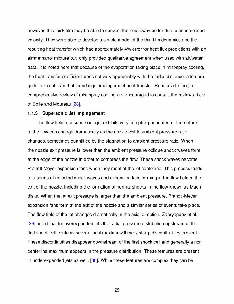
5-8 Results of three separate impulse response experiments. . . . . . . . . . . . . 126

5-9 Inverse method deconvolution results. . . . . . . . . . . . . . . . . . . . . . . . 127

5-10 First order response function comparison. . . . . . . . . . . . . . . . . . . . . . 128

5-11 Best fit results using a first order impulse response function. . . . . . . . . . . . 129

5-12 Comparison of model to deconvolution results. . . . . . . . . . . . . . . . . . . 129

5-13 Best fit results using the model of [114] response function. . . . . . . . . . . . . 130

5-14 Comparison of the 2 exponential model to the deconvolution algorithm results. 131

5-15 Best fit results using the 2 exponential model. . . . . . . . . . . . . . . . . . . . 132

5-16 Biot number distribution showing the effects of Bimax . . . . . . . . . . . . . . . . 134

5-17 Biot number distribution showing the effects of σ. . . . . . . . . . . . . . . . . . 135

5-18 Truncation of Biot number. . . . . . . . . . . . . . . . . . . . . . . . . . . . . . . 137

5-19 Error Contours for L = 10 mm, σDAQ = 0.2 C, and 8 measurement points. . . . 139

5-20 Comparison of the effects of heat gain. . . . . . . . . . . . . . . . . . . . . . . 143

5-21 Centerline NuD results from the inverse heat transfer algorithm. . . . . . . . . . 144

5-22 Spatial NuD results from the inverse heat transfer algorithm. . . . . . . . . . . . 145

A-1 Two-phase NuD results for various Z/D, nominal ReD = 4.46 × 105 . . . . . . . 152

A-2 Two-phase NuD results for various Z/D, nominal ReD 7.27 × 105 . . . . . . . . 153

A-3 Two-phase NuD results for various Z/D, nominal ReD 1.01 × 106 . . . . . . . . 154

A-4 Two-phase NuD results for various liquid mass fractions and Z/D = 2.0. . . . . . 155




A-8 Two-phase φ results for various Z/D, nominal ReD = 4.46 × 105 . . . . . . . . . 159

A-9 Two-phase φ results for various Z/D, nominal ReD 7.27 × 105 . . . . . . . . . . 160

A-10 Two-phase φ results for various Z/D, nominal ReD 1.01 × 106 . . . . . . . . . . 161

A-11 Two-phase φ results for various liquid mass fractions and Z/D = 2.0. . . . . . . 162


11



B-1 Error Contours for L = 5 mm, σDAQ = 0.2 C, and 8 measurement points . . . . 167

B-2 Error Contours for L = 5 mm, σDAQ = 0.2 C, and 16 measurement points . . . 168

B-3 Error Contours for L = 10 mm, σDAQ = 0.2 C, and 8 measurement points . . . 169

B-4 Error Contours for L = 10 mm, σDAQ = 0.2 C, and 16 measurement points . . 170

B-5 Error Contours for L = 10 mm, σDAQ = 1 C, and 8 measurement points . . . . 171

C-1 The 0.33 mm orifice. . . . . . . . . . . . . . . . . . . . . . . . . . . . . . . . . . 172

C-2 The 0.37 mm orifice. . . . . . . . . . . . . . . . . . . . . . . . . . . . . . . . . . 173

C-3 The 0.41 mm orifice. . . . . . . . . . . . . . . . . . . . . . . . . . . . . . . . . . 173

C-4 The 0.51 mm orifice. . . . . . . . . . . . . . . . . . . . . . . . . . . . . . . . . . 174

12

NOMENCLATURE

Variables

A Area [m2]

Bi Biot number = hL/k

C Measurement equation operator

D Diameter [m]

L Lagrangian

M Mach number, Chapter 2

M Total number of measurements

Nu Nusselt number = hL/k

P Pressure [Pa]

R Gas constant for dry air [J/kg K, Chapter 2

R Residual of modeling equation

Re Reynolds number = 4m/π µ D

S Least squares value

T Temperature [C or K]

V Volume [m3]

X Dimensionless relative sensitivity coefficient

cp Specific heat capacity at constant pressure [J/kg K]

f General function

h Heat transfer coefficient [W/m2 K], Chapter 3

h Impulse response function [s]

k Thermal conductivity [W/m K]

13

m Mass flowrate [kg/s]

q′′′ Internal heat generation rate [W/m3]

r Radial coordinate [m]

t time [s]

u Velocity [m/s]

u Dummy variable for partial differential equation, Chapter 4

v Dummy variable for partial differential equation, Chapter 4

w Liquid mass fraction

x Length coordinate [m]

y Width coordinate [m]

y Generalize output variable, Chapter 4

z Height coordinate [m]

Greek letters

α Thermal diffusivity [m2/s]

β Step size for Conjugate Gradient Method

β Grid stretching parameter

γ Ratio of specific heats, Chapter 2

γ Conjugation coefficient for Conjugate Gradient Method, Chapter 4

δ Deflection angle in radians, Chapter 2

δ Thickness [m], Chapter 3

δ Dirac delta function, Chapter 4

ε Stopping criteria value

η Transformed z corrdinate

14

θ Oblique Shock wave angle in radians, Chapter 2

θ Dimensionless temperature

λ Lagrange multiplier, Chapter 4

λ Effective time constant, Chapter 5

µ viscosity [Pa-s]

ξ General parameter to be estimated, Chapter 4

ξ Dummy integration variable, Chapter 5

ρ Density [kg/m3]

τ Dummy variable of integration

τ Time constant [s]

φ Heat transfer enhancement ratio, Chapter 3

φ Dimensionless step response, Chapter 4

ω Humidity ratio

Subscripts

D Solid domain

T Thermocouple measured quantity

a Adiabatic quantity

air Air quantity

exp Experimental measurement

f Fluid quantity

l Liquid quantity

m Measurement quantity

mix Mixture quantity

mod Modified quantity15

o Stagnation quantity, Chapter 2

o Initial quantity, Chapter 4

rms Root-mean-square value

s Surface quantity

sat Value at saturation conditions

sim Simulated measurement

snd Quantity at the speed of sound

v Vapor quantity

w Wall quantity

Superscripts

* Critical quantity, Chapter 2

* Dimensionless quantity

16

Abstract of Dissertation Presented to the Graduate Schoolof the University of Florida in Partial Fulfillment of theRequirements for the Degree of Doctor of Philosophy

A MULTI-PHASE SUPERSONIC JET IMPINGEMENT FACILITY FOR THERMALMANAGEMENT

By

Richard Raphael Parker

May 2012

Chair: James F. KlausnerCochair: Renwei MeiMajor: Mechanical Engineering

This study investigates the heat transfer characteristics of a multi-phase supersonic

jet impingement heat transfer facility. In this facility water droplets are injected upstream

of a converging-diverging nozzle designed for Mach 3.26 air flow. The nozzle is operated

in an overexpanded mode. Upon exiting the nozzle, the high speed air/water mixture

impinges onto a heated surface and provides cooling. Steady state heat transfer

measurements have been performed with peak heat transfer coefficients exceeding

200,000 W/m2. These heat transfer coefficients are on the same order as some of the

highest heat transfer coefficients ever recorded in the literature. Remarkably these heat

transfer coefficients are obtained using liquid flowrates ranging from 0.2 to 0.7 g/s, in

contrast to the several kg/s flowrates seen in studies that produce similarly high heat

transfer coefficients.

During steady state operation it is noted that no evidence of phase change was

experimentally observed. Preliminary investigations indicate that it may not be possible

to obtain evaporative heat transfer in the current facility. In order to investigate this

possibility higher surface temperatures are needed. However, designing a steady state

experiment to achieve high temperature operation is rife with difficulties and is likely to

be prohibitively expensive.

17

In order to overcome these challenges a transient inverse heat transfer (IHT)

method has been developed. One of the important issues revealed during this

investigation is that sensor dynamics will impact the measurements, thus diminishing

the measurement reliability. To alleviate this issue, a method of incorporating sensor

dynamics into the IHT method was developed. This type of method is not explicitly found

in the literature to the author’s knowledge. A method for accurately determining the

impulse response function of the thermocouples used in the transient IHT experiments

yields good experimental results. Heat loss is discovered to be a critical factor in the IHT

method, and a difference in temperature of 3 C between that measured and the ideal

case renders the IHT results unusable.

A parametric study was performed to determine the effects of: disc height, impulse

response function, magnitude and shape of the heat transfer coefficient distribution,

the number of temperature sensors used, and the magnitude of the error in the data

acquisition system. It was discovered that the method was insensitive to noise levels

found in laboratory conditions and the accuracy increases for a decreasing disc height.

The relative slowness of the impulse response functions did affect the accuracy of the

IHT method as long as the time constant of the functions is accurately known.

18

CHAPTER 1INTRODUCTION AND LITERATURE REVIEW

Jet impingement produces high heat transfer coefficients, up to approximately

105 W/m2 -K. Liquid impinging jets have supported some of the highest recorded

surface heat fluxes, ranging from 100 to 400 MW/m2, [1]. Oh et al. [2] and Lienhard

and Hadaeler [3] have studied liquid jets and arrays that can produce heat transfer

coefficients of 200 kW/m2-K. These high heat transfer rates are accompanied by high

liquid flowrates of up to several kg/s of water, and such high water consumption may be

undesirable in some industrial settings. The current study proposes to use a supersonic

multiphase jet impingement facility designed after an experiment by Klausner et al. [4],

which uses the addition of liquid droplets to the impinging air-stream to enhance the

heat removal rate of the supersonic jet. The liquid flowrate will be orders of magnitude

lower than that used by the studies mentioned above, with less than one g/s, which may

be very desirable in applications where minimal water consumption is a concern.

Supersonic two-phase jet heat transfer is a field that has not been previously

studied. The contribution of the current study will largely consist of characterizing the

heat transfer capabilities of such a system including the effects of air and liquid mass

flowrates and nozzle spacing. Additionally, evaporative heat transfer capabilities of the

jet will be studied; in this scenario the latent heat of vaporization could potentially greatly

enhance the heat removal capabilities of the facility. However, it is not known whether

or not liquid evaporation can be achieved due to the high stagnation pressure. Due to

high impact pressures near the jet centerline, phase change is not likely in this region;

however, the conditions far removed from the impingement point may allow phase

change to occur.

19

1.1 Literature Review

Jet impingement heat transfer is a very diverse field and consists of single-phase

heat transfer and evaporative heat transfer, spray/mist cooling, and supersonic jet

impingement heat transfer. A brief review of jet impingement heat transfer is provided.

1.1.1 Single-Phase Jet Impingement

The analytical study of stagnation point flows largely begins with Hiemenz [5] who

studied the flow field of a laminar impinging jet by modifying the Blausis boundary layer

solution. Homann [6] extended this analysis to axisymmetric flows. These flows are part

of the Falkner-Skan boundary layer equations, which take the general form

f ′′′ + βof′′f − β

(1− f ′2

)= 0

where

f (0) = f ′(0) = 0 and f (∞) = 1.

(1–1)

The velocities u and v, and the similarity variable, η, are defined as

u = axf ′ (η)

v = −βo√aνf (η)

η = y

√a

ν,

where a is a proportionality constant and ν is the kinematic velocity of the fluid. Note

that in the radial case the variable x is the radial distance from the origin. The particular

values of β and βo are 1 and 1 for Hiemenz flow and 1 and 2 for Homann flow. The

variable f′′ is proportional to the shear stress, f′ is the non-dimensional velocity u/U∞,

and f is the stream function. Equation (1–1) represents a non-linear ordinary differential

equation (ODE) which must be solved numerically. The shooting type method is

generally used as the value of f′′ is unknown at the origin. The values of f′′ at the origin

20

a

b

Figure 1-1. Solution of a) Hiemenz stagnation point flow and b) Homann stagnationpoint flow.

obtained numerically are 1.2325 for Hiemenz flow and 1.3120 for Homann flow, as found

in [7]. The solution for Hiemenz and Homann flow are shown in Figure 1-1. It is evident

that the the flow fields behave very similarly; however, the free stream velocity and

shear stress are reached for smaller values of the similarity variable for axisymmetric

stagnation point flow. A full derivation of these and other stagnation point flows using

a similarity type approach as that above can be found in the book by Schlichting and

Gersten [8].

21

While the above analysis is sufficient for completely laminar impinging jets, jets

which find industrial application must deal with the boundary layer approaching the free

surface of the jet far removed form the centerline as well as the transition to turbulence.

Due to the different flow regimes the jet analysis is typically broken up into several

different regions and analyzed through the use of a von Karmam momentum integral

analysis; for an analysis of stagnation region see [9].

The analysis of the temperature field within the boundary layer for these types of

flows is complicated due to the behavior of the thermal boundary layer that develops

on the surface. It is further complicated by the nature of the fluid itself as flows with

larger Prandlt (Pr) number behave very differently than flows with small ones. As the

boundary layer moves away from the centerline, the hydrodynamic boundary layer

reaches the free surface before the thermal boundary layer for Pr < 1 while the converse

is true for Pr > 1. Liu et al. have analyzed the flow in each of these regions for single

phase jets with constant surface temperature and heat fluxes, mostly through the use

of the von Karman-Pohlhausen integral solution [10, 11]. They were able to model the

transition to turbulence and the subsequent turbulent flow as well. Their solutions agree

exceptionally well with experimental results. In general the solutions have the form of

The analysis of the above flow field is not limited to integral solutions or to constant

boundary conditions. Wang et al. [12, 13] studied the effects of a spatially varying

surface temperature and heat flux on the solution using a perturbation method. They

found that the direction of increasing temperature affects the Nusselt number of the

flows, notably that increasing the wall temperature or heat flux with radial distance

from the origin will decrease the Nusselt number in the stagnation zone. Conversely

it increases the Nusselt number in the boundary layer region. Wang et al. additionally

studied the conjugate heat transfer problem where the temperature field is determined in

the liquid and solid simultaneously, [14]. They found that thickness of the heater can be

a contributing factor for the heat removal capability of the jet.

22

There are several additional phenomena that impact the cooling rates of impinging

jets. These include the effects of the jet nozzle diameter [15], hydraulic jump [16], and

the splattering of liquid from the resulting free surface [17]. In cases with sufficiently high

surface temperature, phase change can be observed under impinging jets including the

regions of nucleate boiling, departure from nucleate boiling, and transition boiling [18].

While most studies of liquid jet impingement find no appreciable effect on the nozzle

height above the heat surface, Jambunathan et al. [19] noted that some studies do show

an effect most notably at higher Reynolds numbers. An empirical correlation based

on heat transfer data available in the literature was proposed however, it provides no

physical insight of the flow field and heat transfer taking place.

Liquid jet impingement can support exceptionally high surface heat fluxes. Liu and

Lienhard [1] used a liquid jet with velocities exceeding 100 m/s, liquid supply pressures

of up to approximately 9 MPa, and flowrates of approximately 300 g/s to remove heat

fluxes of at least 100 MW/m2. These experiments were novel in the fact that they used

a plasma torch as a heat source. Surface temperatures were determined by coating

the top surface with a material of known melting temperature and completing several

experimental runs until the surface temperature could be isolated to lie within a range

of temperatures. Melting of the heated surface occurred due to the use of the torch and

the back wall temperature was assumed to be essentially the melting temperature of

the solid. The heat flux was determined by using the minimum thickness of the solid

where it had melted and then assuming a linear temperature profile. Because of the

coarse nature of the measurements, uncertainty is hard to quantify and heat transfer

coefficients were not reported. However, the heat fluxes measured are the highest

steady state valuesrecorded in the literature. To further enhance the study of high heat

flux removal Michels, Hadeler, and Lienhard [20] and Lienhard and Napolitano [21]

designed thin film heaters using vacuum plasma spraying and high velocity oxygen

fuel spraying. These heaters are supplied with dc electrical power of up to 3,000 A and

23

24 V, producing heat fluxes of up to 17 MW/m2. Lienhard and Hadeler [3] were able

to construct an array of liquid jets with liquid supply pressures of approximately 2 MPa

and flowrates of approximately 4 kg/s. These impinging jet arrays were able to support

heat fluxes of 17 MW/m2 with an average heat transfer coefficient of 200 kW/m2 with

uncertainties of ±20%. Similar results were found in a study by Oh et al. [2]. These

studies help illustrate the high heat removal capabilities of jet impingement technology.

For an extensive review of the subject of liquid jet impingement the author

recommends the review articles of Liendhard [22], Webb and Ma [23], and Martin

[24]. These articles offer a complete review of the subject and include many effects not

discussed in this brief literature survey.

1.1.2 Mist and Spray Cooling

Mist/spray cooling of a heated surface is largely different from jet impingement due

to the fact that the liquid impinging on the surface is in the form of disperse droplets.

These droplets are usually generated by forcing liquid through very small orifices

within a nozzle which atomizes the liquid. The primary benefit of using this technique

is that the disperse droplets generally allow for evaporative heat transfer to dominate.

Mist/spray cooling produces heat transfer coefficients on the order of those found during

pool boiling. However, the critical heat flux can be several times higher [25].

The droplet size is an important parameter in mist/spray cooling, Estes and

Mudawar [26] correlated the critical heat flux (CHF) with the Sauter mean diameter

of the sprays; they also found that the apparent density of the spray can be an important

factor in mist/spray cooling as denser sprays are less effective. Mist/spray cooling

can also be applied to surfaces lower than the boiling point of the liquid. The reduced

evaporation can lead to a buildup of a liquid film on the heated surface which can have a

thickness less than the size of the droplets. Graham and Ramadhyani [27] performed an

experimental study which shows that increasing the amount of droplets on the surface

can lead to thicker films which may increase the thermal resistance at the surface;

24

however, this thick film may be able to convect the heat away better due to an increased

velocity. They were able to develop a simple model of the thin film dynamics and the

resulting heat transfer which had approximately 4% error for heat flux predictions with an

air/methanol mixture but, only provided qualitative agreement when used with air/water

data. It is noted here that because of the evaporation taking place in mist/spray cooling,

the heat transfer coefficient does not vary appreciably with the radial distance, a feature

quite different than that found in jet impingement heat transfer. Readers desiring a

comprehensive review of mist spray cooling are encouraged to consult the review article

of Bolle and Moureau [28].

1.1.3 Supersonic Jet Impingement

The flow field of a supersonic jet exhibits very complex phenomena. The nature

of the flow can change dramatically as the nozzle exit to ambient pressure ratio

changes, sometimes quantified by the stagnation to ambient pressure ratio. When

the nozzle exit pressure is lower than the ambient pressure oblique shock waves form

at the edge of the nozzle in order to compress the flow. These shock waves become

Prandtl-Meyer expansion fans when they meet at the jet centerline. This process leads

to a series of reflected shock waves and expansion fans forming in the flow field at the

exit of the nozzle, including the formation of normal shocks in the flow known as Mach

disks. When the jet exit pressure is larger than the ambient pressure, Prandtl-Meyer

expansion fans form at the exit of the nozzle and a similar series of events take place.

The flow field of the jet changes dramatically in the axial direction. Zapryagaev et al.

[29] noted that for overexpanded jets the radial pressure distribution upstream of the

first shock cell contains several local maxima with very sharp discontinuities present.

These discontinuities disappear downstream of the first shock cell and generally a non

centerline maximum appears in the pressure distribution. These features are present

in underexpanded jets as well, [30]. While these features are complex they can be

25

Figure 1-2. An illustration of the shock structure in the wall jet region. [Reprinted withpermission from Carling, J. C. and Hunt, B. L., The Near Wall Jet of aNormally Impinging, Uniform, Axisymmetric, Supersonic Jet, Journal of FluidMechanics 66 (1974) 159–176 (Page 174 Figure 9(b)), Cambridge UniversityPress]

modeled somewhat accurately by a method of characteristics approach as noted by

Pack, [31, 32] and Chu [33], among others.

Underexpanded impinging jets have been extensively studied in the literature

as they pertain to the launching of rockets and spacecraft, whereas overexpanded

impinging jets are relatively uncommon in industrial settings. When a jet impinges

upon a flat plate, a complex shock structure is formed. This shock structure forms

several complex features including a triple shock structure, where three shock waves

intersect near the impingement surface, a bow shock, also known as a plate shock in

the literature, as the flow must come to rest in the stagnation point on the surface, and

the shock waves which radiate from the triple shock point and slow the flow along the

plate to subsonic speeds. These features appear in all types of supersonic impinging

jets including underexpanded, ideally expanded, and overexpanded. The bow shock, if

curved, can form a recirculating stagnation region in the area of the center of the jet to

the edge of the nozzle. An illustration of the complex shock structure of the flow at larger

radial distances along the impingement plate is shown in Figure 1-2.

The stagnation region is very complex due to the formation of the above mentioned

bow shock and stagnation bubble. Donaldson and Snedeker [30] studied underexpanded

jets from a converging nozzle and performed many different measurements to help

26

characterize some of the important features of the flow including impingement angle

and nozzle pressure ratio. They were able to observe stagnation bubbles forming, but

noted that this phenomenon did not occur in every experiment. Schlieren photographs

were taken as well as total pressure measurements along the jet centerline, and it was

observed that the velocity and pressure vary greatly in the axial direction. The velocity

in the radial wall jet region was measured via the use of pitot-static pressure tube

measurements along the impingement surface, the effects of surface curvature were

also characterized. Gummer and Hunt [34] also studied the flow of uniform axisymmetric

ideally expanded supersonic jets with low nozzle to height spacing and noted the

presence of the bow shock and complex shock structure in the wall jet region. They

attempted to use a polynomial and integral relation method to model the bow shock

height and the pressure distribution under the nozzle. Some success was seen for high

Mach numbers but not in the region of the triple shock. Low Mach number calculations

contained as much as 60% error. Carling and Hunt [35] performed a theoretical and

experimental investigation using the nozzles of Gummer and Hunt. Their study mostly

comprised of the region just outside of the nozzle along the impingement plate. They

were able to note the presence of the stagnation bubble for some of their experiments,

but not all. The presence of the stagnation bubble can severely influence the pressure

distribution on the plate and an annular maximum is possible for some jet spacings.

Attempts were made to model the shock structure in the wall jet region using the method

of characteristics. Qualitative features of the flow were able to be reproduced. However,

there appears to be some error in the region near the triple shock region. The pressure

variation along the plate was measured which showed several regions of unfavorable

pressure gradient. Carling and Hunt were able to investigate these regions by coating

the impingement plate with a type of grease. When the jet is impinged upon the plate

these unfavorable pressure gradients cause the grease to be removed due to local

separation of the boundary layer. A photograph of one of these experiments is shown

27

Figure 1-3. Grease streak type photograph from [35], the dark areas contain no greaseand are areas of high wall shear stress. [Reprinted with permission fromCarling, J. C. and Hunt, B. L., The Near Wall Jet of a Normally Impinging,Uniform, Axisymmetric, Supersonic Jet, Journal of Fluid Mechanics 66(1974) 159–176 (Plate 3 Figure 6(d)), Cambridge University Press]

in Figure 1-3. The dark regions represent where no grease is present; note the very

dark region near a radial distance of 2 nozzle diameters from the center where evidence

of separation is clearly evident. The separation phenomenon was noted by several

investigators including Donaldson and Snedeker, [30]. Kalghatgi and Hunt provide a

qualitative analysis experimental study of overexpanded jets which concentrated on the

triple shock problem near the edge of the bow shock. Their analysis suggests that flat

bow shocks are a possibility and schlieren photographs of overexpanded impinging

jets with Mach numbers ranging from approximately 1.5 to 2.8 largely confirmed

their qualitative analysis. They also note that the formation of a flat bow shock is a

phenomenon that is hard to predict. Lamont and Hunt performed a comprehensive

experimental study on underexpanded jets oriented normally and obliquely to a flat plate

which includes pressure measurements and schlieren photographs. The stagnation

bubble phenomenon was noted as well as some unsteadiness in the jet. Velocity and

pressure profiles were seen to vary greatly with the nozzle to plate distance, and it was

noted that the local shock structure has a strong influence on the flow field.

28

Unsteadiness of the impinging jet is caused by a feedback phenomenon which

has been extensively studied due to its importance in air vehicle takeoff, including the

launching of rockets and short/vertical take off and landing vehicles, such as the Joint

Strike Fighter. This mechanism was successfully modeled by Powell, [36, 37]. The

mechanism is caused by acoustic phenomena occurring at the edge of the nozzle.

These acoustic waves cause vortical structures to be generated in the shear layer

of the jet and are convected towards the impingement point. Upon encountering the

region near the plate, these structures interact with the shock waves near the plate

generating strong acoustic waves, which travel upstream towards the nozzle where were

they interact with the nozzle edge generating more acoustic waves which then repeat

the process [38]. Krothapalli [39] was able to predict the frequencies generated by a

supersonic impinging rectangular jet using Powell’s model, thus validating the theory.

The effects of the unsteadiness on the flow field will be detailed below.

Due to the complex shock structure and unsteady phenomena in impinging jets,

numerical simulations are often used to help enhance the knowledge in this area. Alvi et

al. [40] modeled the impingement of moderately underexpanded jets and used Particle

Image Velocimetry (PIV) to help verify their results. Their method had reduced temporal

accuracy, but was able to reproduce major flow features including the stagnation bubble

and wall jet region, although the region of the triple shock point had some disparity

between the numerical and experimental results. Klinkov et al. [41] compared numerical

results of the velocity, pressure, and density fields to experimental results in the form

of schlieren photographs and surface pressure measurements. Their study focused

on overexpanded jets with Mach numbers in the range of 2.6 to 2.8 at approximately

ambient stagnation temperatures. They found that the location of the bow shock can

change significantly with nozzle to plate spacing, with several regions of a near constant

shock height followed by an almost discontinuous change to another height. Regions

of high shock height represent a convex bow shock and regions of low shock height

29

represent a flat bow shock with unsteadiness noted as the shock transforms to from

a convex shock to a flat shock. They also noted that a stagnation bubble region is

typical of a convex bow shock and that regular stagnation flow accompanies a flat

bow shock. An illustration is shown in Figure 1-4. The behavior of the bow shock is

significantly affected by the unsteady feedback mechanism as it is seen to oscillate back

and forth along the axis of the jet. This causes correspondingly large fluctuations in the

surface pressure on the impingement plate. Kawai et al. performed a computational

aeroacoustic study which was 2nd order accurate in time and 7th order accurate in

space. This study was done to determine the effects of the presence or absence of

a hole in a launch pad configuration and primarily focused on large nozzle to plate

spacings and the effect of Reynolds number on the unsteady phenomena. It was seen

that high Reynolds numbers can significantly increase the sound power levels of the

jet and the magnitude of its oscillations. Their numerical code produced results which

agreed well with historical sound power level data maintained by NASA. This study is

useful in illustrating the complexity of the problem under study and how very complex

numerical simulations are needed to accurately reproduce the features of the flow.

The addition of moisture in the form of water vapor to the air supply of an impinging

jet can have a noticeable impact on the flow field. This was observed experimentally by

Baek and Kwon [42] who performed studies of air with varying degrees of supersaturation

of water vapor for a supersonic jet issuing into quiescent air. They found that the

location of the Mach disk was located further upstream in the flow for moist air jets

and its size was reduced. Empirical correlations for the location of quantities such

as the size and location of the Mach disk and the location of the jet boundary were

proposed, although little mechanistic insight to the flow was gained. Numerical studies

by Alam et al. [43, 44] and Otobe et al. [45] were performed for air with various values

of supersaturation of water vapor for a supersonic jet impinging on a flat plate. They

attempted to model the non-equilibrium condensation taking place in the region after the

30

Figure 1-4. Numerical results of a flow field with a flat plate shock (left) and curved flatplate shock (right). [Reprinted with permission from Klinkov K. et al,Behavior of Supersonic Overexpanded Jets on Plats, in: H.-J. Rath, C.Holze, H.-J. Heinemann, R. Henke, H. Hnlinger (Eds.), New Results inNumerical Fluid Mechanics V, volume 92 of Notes on Numerical FluidMechanics and Multidisciplinary Design, Springer, 2006, pp. 168–175 (Page173 Figure 3]

first Mach disk in the flow. Their model assumes no slip between the liquid droplets that

condense and that these droplets do not influence the pressure of the flow downstream.

The flow field displays some noticeable differences than that of dry air. The authors

propose that this is due to the addition of the latent heat of condensation to the air by the

condensing water vapor. Unsteady behavior due to the acoustic feedback mechanism

by Powell was seen in the simulations. This unsteadiness was not present upstream

of the first Mach disk, but was seen down stream of it. The presence of condensate

particles combined with the addition of the latent heat reduces the magnitude of the

pressure fluctuations seen in the downstream portion of the flow which is illustrated in

Figure 1-5. The authors attempted to verify their simulations with experimental data,

31

a b

Figure 1-5. Jet centerline pressure fluctuations with a) no moisture and b) 40%supersaturation of water vapor. [Reprinted with permission from AshrafulAlam, M. M. et al., Effect of Non-Equilibrium Homogeneous Condensationon the Self-Induced Flow Oscillation of Supersonic Impinging Jets,International Journal of Thermal Sciences 49 (2010) 2078–2092 (Page 2086Figure 10(b) and Page 2088 Figure 13(c)), Elsevier]

mostly consisting of comparing the shock structure as seen in schlieren photographs like

those in the study by Baek and Kwon, along with noise tones for dry air generated by the

acoustic feedback mechanism. This proposed validation is weak because there is a lack

of experimental data of which to compare to in the literature.

The study of supersonic impinging jet heat transfer jets has been studied extensively

in the literature. Unfortunately most of these studies have focused on the heat transfer

from a rocket exhaust to a launch pad facility. Donaldson et al. [46] performed an

experimental study of impinging sonic jets and their turbulent structure. The authors

were able to develop a correlation for Nusselt number based on applying a turbulent

correction factor to laminar impinging jet theory near the stagnation point and further

away in the wall jet region. While good agreement was found for their correlation it

is for sonic or just slightly supersonic impinging jets and does not apply to the highly

32

supersonic jets previously mentioned. The unsteady acoustic feedback phenomenon

previously discussed causes interactions between acoustic waves and the shock

structure of the impingement region. This results in local cooling to occur in the

region of the jet edge and is very noticeable in the measurement of the adiabatic wall

temperature. This phenomenon is termed cooling by shock-vortex interaction by Fox and

Kurosaka [47] who investigated this phenomenon. Kim et al. [48] studied the surface

pressure and adiabatic wall temperature of an underexpanded supersonic impinging

jet. They noted that the acoustic vortical structure interaction significantly affects the

adiabatic wall temperature and surface pressure which also varies greatly with nozzle

height. The presence of a stagnation bubble, which enhances the cooling directly below

the nozzle, was noted as well. Rahimi et al. studied the heat transfer of underexpanded

impinging jets onto a heated surface. The temperature of the impingement surface with

uniform applied heat flux is noted to change dramatically with radial distance as well

as with nozzle spacing as shown in Figure 1-6. They note that Nusselt number scales

approximately with the square root of Reynolds number and that high heat transfer rates

are encountered in the stagnation zone when a stagnation bubble is present. Due to the

complexity of the problem, they note that a general correlation of Nusselt number should

be a function of not only Reynolds number and Prandtl number, as is common, but also

a function of Mach number and nozzle spacing. Yu et al. performed a similar study and

noticed similar trends; their measured Nusselt numbers exceed 1,500.

Studies of the heat transfer characteristics of supersonic moist impinging jets

are not found in the literature. They are likely to show very complex phenomena

as evidenced by the differences in the shock structure and general behavior of the

relevant flow quantities in the jet and along the impingement plate. The current study

uses discrete liquid droplets that are injected into the air upstream of the nozzle.

This will likely result in an air stream supersaturated with water vapor which is further

complicated by the behavior of the liquid droplets and their effects on the flow. As

33

a b

Figure 1-6. Adiabatic (circles) and heated (diamonds) wall temperature for a nozzlespacing of a) z/D = 3.0 and b) z/D = 6.0. [Reprinted with permission fromRahimi M. et al, Impingement Heat Transfer in an Under-ExpandedAxisymmetric Air Jet, International Journal of Heat and Mass Transfer 46(2003) 263–272 (Page 267 Figures 6(a) and 6(b)), Elsevier]

elucidated by the literature survey the flow structure associated with this technology is

very complex, and essentially no analytical solutions are available for the flow field and

heat transfer. The available empirical correlations do not cover two-phase supersonic

impinging jets. Numerical studies may provide some qualitative insight, but in most

instances they do not adequately capture all of the physics taking place in the flow field.

1.2 Summary

In this Chapter an introduction to the study was made and the relevance of

multiphase supersonic impinging jets was introduced. The contributions of this study

were also described, mainly that this is a technology that has not been studied until now.

A brief literature review of the different types of impingement heat transfer was

presented. Liquid and single-phase heat transfer was introduced starting with the

classic work of Hiemenz and Homann. The development of accurate Nusselt number

correlations based on von Karman-Pohlhausen integral method were detailed. The

agreement between theory and experiments is exceptional for these correlations.

Other aspects such as the flow hydrodynamics, transition to turbulence, nozzle height,

34

and non-uniform boundary conditions effects were discussed. High heat flux removal

technologies that are capable of heat transfer coefficients as high as 200 kW/m2 were

detailed as well.

The study of supersonic underexpanded and overexpanded impinging jets was

described as well. This field is complicated by the complex flow structure generated by

shock waves which form when a nozzle is operated away from its designed pressure

ratio. The details of these shock waves including the effects of the curvature of the

bow shock just above the impingement plate were discussed. Stagnation bubbles

formed just below the bow shock were discussed and their impact on the flow field

was detailed as well. Shock waves near the impingement region cause an unsteady

feedback phenomenon caused by the interaction of acoustic waves with the edge of

the nozzle. The effects of this feedback phenomenon and the unsteadiness it causes

and relevant changes in the local flow field were detailed. Moisture in the air stream and

how it changes the relevant flow field was briefly explored as it is a relatively new area

of study in the literature. The temperature profile on the impingement plate and how it

changes with the presence of the stagnation bubble and acoustic feedback mechanism

were discussed. Numerous experimental studies in the literature which include pressure

and temperature measurements, particle image velocimetry, and schlieren photographs

along with relevant numerical studies in the literature that discovered and confirmed

these phenomena were discussed where relevant.

Lastly the complexity of the current study was discussed. It is noted that an

analytical solution to the problem will not be attainable and a predictive numerical study

is not feasible as well. The contributions of this study will be in the form of developing

an understanding of the mechanisms taking place as the multiphase supersonic jet

removes heat from a surface.

35

CHAPTER 2JET IMPINGEMENT FACILITY

The supersonic multi-phase jet facility should possess several traits in order to be

useful for an experimental apparatus. It should have sufficient air storage capacity so

that experiments can be run at steady state. The stored air should be pressurized to

such an extent that the desired Mach number can be achieved. Lastly it should contain

sufficient water, and a means to control the flow, so that the impinging jet will remain in

multiphase operation during experiments.

The design for the current setup is based on a similar experiment by Klausner et

al. [4]. The impinging jet consists of the following systems to be described below: air

storage system, water storage and flow control system, air pressure control system,

air mass flowrate measuring system, temperature and pressure measurement system,

converging-diverging nozzle, and data acquisition system (DAQ). A schematic diagram

illustrating the configuration of the jet impingement facility is shown in Figure 2-1.

2.1 Impinging Jet Facility Systems

2.1.1 Air Storage System

The air storage system consists of 9 ‘K’ sized bottles which give a total volume of

0.45 m3 and are kept at a pressure of 14 MPa. The air storage system is filled with air

from a model UE-3 compressor from Bauer Corporation. The compressor is powered by

a 3-phase 240 V power supply and is capable of supplying 0.1 m3/min of approximately

moisture free air to the air cylinders, thus the air storage facility can be charged to

capacity in approximately 4.5 hrs.

2.1.2 Water Storage and Flow Control System

Water for the facility is contained in a stainless steel vessel with a capacity of 2

L and a pressure rating of 12.4 MPa. Water is forced into the mixing chamber by the

difference in pressure between the top of the water vessel (which is acted on the the full

force of the air supply pressure) and the pressure inside the mixing chamber, which is

36

Figure 2-1. Illustration of the jet impingement facility.

lower due to a change in area and because of the friction acting in the system tubing. A

drawing the of the mixing chamber is found in Figures 2-2 and 2-3. The flowrate of the

water is controlled by means of an orifice between the water vessel and mixing chamber

and the air pressure in the system. Orifice diameters of 0.33, 0.37, 0.41, and 0.51 mm

are used during experiments, and a drawing of the orifice design is found in Figure 2-4.

While there is some variance in flowrate between each experiment for a given orifice

size this effect is eliminated in the analysis due to the fact the the flowrate of water

into the mixing chamber is measured during each experiment. This is accomplished

by recording the elapsed time of each experiment and measuring the difference in the

mass of liquid in the water vessel. Table 2-1 shows the nominal flowrate of liquid and the

37

Figure 2-2. Cross section of the mixing chamber.

Figure 2-3. Thread details of the mixing chamber cross section.

average liquid velocity for the pressures and orifice sizes used during the experiments. It

is noted that the flowrate of the 0.37 mm orifice is less than that of the 0.33 mm orifice,

this is due to the fact that the 0.37 mm orifice is not perfectly circular. This condition is

also seen in the 0.51 mm orifice, but it is not as severe as that in the 0.37 mm orifice.

Pictures of each orifice taken with an optical microscope are shown in Appendix C.

38

Figure 2-4. Orifice cross section.

2.1.3 Air Pressure Control System

The air pressure control system consists of an air regulator located between

the air storage tanks and the inlet to the air mass flowmeter and the top of the water

storage tank. The regulator is capable of reducing air pressure from 14 MPa down

to a maximum of 2.8 MPa. Air pressures of 1.0, 1.7, and 2.4 MPa are used during

experiments. As discussed later, these air pressures result in the converging-diverging

nozzle operating in an overexpanded manner.

2.1.4 Air Mass Flow Measuring System

Measurement of the air mass flowrate is accomplished using an Annubar Diamond

II model DNT-10 mass flowmeter located downstream of the regulator and before the

mixing chamber. The diamond cross section of the flowmeter is such that it has a fixed

separation point and also reduces pressure loss. The flowmeter senses differential

pressure which is measured with a differential pressure (DP) transducer, which is

39

Table 2-1. Water Mass Flowrate and Average Water Velocity for Different RegulatorPressures and Orifice Sizes.

Orifice Regulator Water Mass Average WaterSize Pressure Flowrate Velocity(mm) (MPa) (kg/s) (m/s)

1.0 3.08 x 10−4 3.600.33 1.7 3.99 x 10−4 4.67

2.4 4.73 x 10−4 5.53

1.0 2.67 x 10−4 2.500.37 1.7 3.31 x 10−4 3.11

2.4 3.97 x 10−4 3.73

1.0 4.61 x 10−4 3.550.41 1.7 5.72 x 10−4 4.41

2.4 6.79 x 10−4 5.24

1.0 4.85 x 10−4 2.390.51 1.7 6.90 x 10−4 3.00

2.4 7.20 x 10−4 3.55

calibrated to measure pressure differences of up to 2.21 × 10−3 MPa. The calibration

equation for the flow meter is

m = 58.283KD2√

∆Pρf (2–1)

where ∆ P is the measured differential pressure in kPa, D is the diameter of the

flowmeter in mm, in this case 15.80 mm, K is a gage factor of 0.6, and ρf is the density

of the flowing air, in kg/m3 calculated via

ρf = 539.5PfTf

(2–2)

where Pf is the pressure of the flowing air in kPa, as measured by the pressure

transducer upstream of the mass flowmeter and Tf is the temperature of the flowing

air in Kelvin as measured by the the thermocouple upstream of the mass flowmeter.

40

Figure 2-5. A comparison of the theoretical and experimentally measured air massflowrate.

The theoretical mass flowrate through the nozzle for 1-D isentropic flow is

calculated using mass flow, m = ρAV, the Mach number, M = a/V (the speed of sound for

a perfect gas is a =√γRT), and the ideal gas law, P = ρRT,

m =π

4D2MP

√γ

RT(2–3)

Knowing that at the throat of the nozzle the Mach number is one and using

Temperature and Pressure stagnation ratios of T/To = 0.8333 and P/Po = 0.5282

Equation (2–3) reduces to

m = 0.4545D2Po

√γ

RTo(2–4)

41

Equation (2–4) neglects the effects of friction and heat transfer, which affect the flowrate

of air through the nozzle. A comparison of the air mass flowrate measured during the

course of experiments with the theoretical air mass flowrate is shown in Figure 2-5. The

agreement between theory and experiment is within 20%.

2.1.5 Temperature and Pressure Measurements

The temperature and pressure of the jet impingement system is monitored during

system operation for calculating various quantities of interest. The temperature

measurements are accomplished by the use of E type thermocouple probes which

are inserted into ‘T’ junction compression fittings at a depth such that the tip of the

probe is at the centerline of the fitting. The thermocouple probes used are grounded

and sheathed in stainless steel and have a nominal diameter of 1.59 mm. Temperature

measurements are taken at the following points: the outlet of the pressure regulator, the

outlet of the water reservoir, and at the outlet of the mixing chamber.

Pressure is measured at the outlet of the pressure regulator just before the location

of the air mass flowmeter. The pressure measurement is made using a strain gage

type pressure transducer, which has a range of 0 - 2.8 MPa. The output signal of the

pressure transducer is a current which varies between 4 - 20 mA; because the DAQ

system used in the experiments only senses voltages a resistor of 520 Ω is used to

convert this current into a voltage in the 0 - 10 V range needed.

2.1.6 Converging-Diverging Nozzle

The converging-diverging nozzle is where the mixture of liquid and air are expanded

to supersonic speeds. The nozzle is constructed of stainless steel with a throat

diameter of 2.38 mm and an exit diameter of 5.56 mm, giving an exit Mach number

of 3.26. The nozzle is attached to a size 10 DN (1/2” NPS) stainless steel pipe with an

internal diameter of 13.51 mm, which is connected to a braided stainless steel hose

approximately 9 m long with an inner diameter of 9.53 mm and is connected to the

outlet of the mixing chamber. Although the hose adds some small amount of pressure

42

Figure 2-6. Cross sectional view of the converging-diverging nozzle used inexperiments.

loss, it allows the nozzle to be located away from the air storage cylinders and near

the impingement heat transfer targets. A cross sectional view of the nozzle is shown in

Figure 2-6.

2.1.7 Data Acquisition System

The DAQ used during the course of steady state heat transfer experiments is a

DAS - 1601 data acquisition PCI card and a CIOEXP32 analog to digital converter

board, both made by Measurement and Computing Inc. This DAQ consists of 32 16-bit

double ended channels and channel gains of 1, 10, 100, 200, and 500 are selectable.

The system has a maximum reliable sampling rate of 50 Hz and the software Softwire,

produced by Measurement and Computing Inc is used for programming data collection.

For transient measurements on heated targets during inverse heat transfer experiments,

the DAQ system is supplemented with a National Instruments (NI), NI USB-6210 system

which has 8 double ended 16-bit channels and has a maximum aggregate sampling rate

of 250 kHz. This system uses Labview software produced by NI which and is also able

43

to interface with the Measurement and Computing DAQ via the use of an NI supplied .dll

library.

2.2 Analysis of Impingement Facility

Some analysis of the jet impingement facilities are warranted. The behavior of the

system upstream of the nozzle is examined to determine if there are any corrections that

need to be applied to the thermocouple or pressure transducer readings. Additionally,

the following is examined: the pressure required to operate the nozzle in a perfectly

expanded manner, the minimum and maximum pressure that cause a shock wave

to form inside the nozzle, and the nozzle exit pressure when operating at various

regulator pressures. Lastly the shock wave angles forming at the nozzle exit for various

operating pressure are calculated as well. One-dimensional gas dynamic relations are

used to investigate the quantities of interest. Here it is noted that the analysis used

has limitations, the one dimension gas dynamic relations are isentropic in nature, with

the exception of shock wave calculations. The jet impingement facility experiences

friction and heat transfer during operation, thus the isentropic assumption is not met.

Additionally after the mixing chamber the flow will contain water droplets which are not

compressible. The quantities calculated below will have some inherent error however,

they do provide a reasonable approximation of the physics taking place in the facility.

2.2.1 Temperature and Pressure Upstream of the Nozzle

Calculating the temperature and pressure at various points upstream of the nozzle

is a simple matter; the cross-sectional area of the points in the system are required for

this analysis; Figure 2-7 provides an illustration of the jet impingement facility and the

diameters of the points of interest. Using the commonly known one-dimensional gas

dynamics relationships found in various compressible flow textbooks, such as Liepmann

and Roshko [49] or John and Keith [50], the pressure and temperature ratios as well

as the Mach number of the flow in these areas can be determined. In the following

44

Figure 2-7. Simplified view of the air flow path in the facility.

equations γ is the ratio of specific heats and is a constant equal to 1.4. To determine the

flow Mach number the following relationship is used

A

A∗=

1

M

[(2

γ + 1

)(1 +

γ − 1

2M2

)] γ+12(γ−1)

(2–5)

where the * superscript denotes the critical area where Mach = 1. Note that Equation (2–5)

is a quadratic equation in M and has two solutions thus careful attention must be paid

in selecting the proper Mach number given an area ratio, in the present case all Mach

numbers upstream of the throat of the converging-diverging nozzle are subsonic. Once

45

the Mach number of the given section is determined the pressure and temperature ratios

can be determined from the following

ToT

= 1 +γ − 1

2M2 (2–6)

PoP

=

(1 +

γ − 1

2M2

) γγ−1

(2–7)

where the subscript o is the stagnation property, which is simply the particular property

with zero velocity. The analysis results using Equations (2–5) to (2–7) are shown in

Table 2-2. The results show that the temperature and pressure upstream of the nozzle

throat differ from their stagnation point properties by less than 1%; no correction due the

the velocity of the flow is needed.

Table 2-2. Area, temperature, and pressure ratios at various points in the jetimpingement facility.

Point A/A∗ T/To P/Po M

Exit 5.44 0.3193 0.01840 3.26Throat 1.00 0.5283 0.8333 1.00

1 32.20 0.9999 0.9998 0.0182 6.83 0.9986 0.9950 0.0853 44.02 0.9999 1.0000 0.0134 6.83 0.9986 0.9950 0.085

2.2.2 Nozzle Exit Pressure Considerations

There are a few theoretical considerations that need to be explored at the nozzle

exit. First, the necessary regulator pressure in order to obtain a perfect expansion at the

nozzle exit is needed; then the actual exit pressures based on the regulator pressure

during experiments are determined. The results from the previous calculations listed in

Table 2-2 show the stagnation pressure ratio at the exit of the nozzle, simply carrying

the requisite algebra and assuming a back pressure of 101.4 kPa yields the nozzle

exit pressure, see the results of these calculations in Table 2-3. From these results it

is observed that the pressure necessary for ideal expansion is approximately twice the

46

pressure the regulator of the system can provide, and thus during normal operation of

the jet impingement facility the nozzle operates in an overexpanded manner.

Table 2-3. Nozzle exit pressure for various regulator pressures.

Regulator Nozzle Exit NozzlePressure Pressure Operation

(MPa) (MPa)

5.5 0.1014 perfectly expanded2.8 0.0508 overexpanded2.4 0.0443 overexpanded1.7 0.0317 overexpanded1.0 0.0190 overexpanded

Due to the fact that the nozzle exit pressure is below the ambient pressure some

concern about a shock wave forming in the nozzle will be addressed. There are two

limiting pressures for this case, one is the pressure at which at shock wave forms at the

throat of the nozzle, the other is the pressure that a shock wave forms at the nozzle exit;

Figure 2-8 shows an illustration for both of these two cases. In the limiting case, a shock

wave occurring at the throat (where the Mach number is equal to unity), the stagnation

pressure ratio is 0.992. Assuming that the back pressure is atmospheric pressure, the

stagnation pressure that will cause a shock to be located at the throat is 0.102 MPa. To

calculate the limiting case of a shock wave occurring at the nozzle exit is just slightly

more complicated. When it is assumed that a shock wave is located at the exit plane of

the nozzle, the stagnation pressure ratio and Mach number just before the exit plane can

be found from Table 2-2. The normal shock wave relations for Mach number and static

pressure ratio across a shock (Equations (2–8) and (2–9)) can then be applied,

M2 =

√M2

1 (γ − 1) + 2

2γM21 − (γ − 1)

(2–8)

P2

P1

=2γM2

1

γ + 1− γ − 1

γ + 1. (2–9)

47

Figure 2-8. Illustration of the limiting cases for shock waves in the nozzle.

Using Equations (2–8) and (2–9) the Mach number just past the shock wave is

found to be 0.461 and the static pressure ratio is 12.268. Performing the requisite

algebra yields a back pressure of 0.449 MPa. Thus the nozzle will have a shock wave

located inside for a stagnation (regulator) pressure in the range of 0.102 to 0.449 MPa.

Since the minimum regulator pressure used during experiments is 1.0 MPa there is little

concern that a shock wave will form inside the nozzle.

2.2.3 Oblique Shock Waves at Nozzle Exit

It is known that the converging diverging nozzle operates in an overexpanded

manner; the exit conditions of the nozzle should be considered. When a nozzle

is overexpanded oblique shock waves form at the outlet of the nozzle, see [49] for

instance. These shock waves compress the air such that it is then equal to the

nozzle back pressure; the first oblique shock wave coming out of the nozzle can be

modeled using the standard one dimensional gas dynamic relations parameters such

as the shock angle, deflection angle, temperature ratio, stagnation pressure ratio, and

down stream Mach number. Figure 2-9 shows an illustration of the shock wave at the

nozzle exit. To determine these exit quantities, first the nozzle exit pressure should be

determined using the regulator pressure and Equation (2–7). The shock wave angle can

48

Figure 2-9. Illustration of an oblique shock wave at the nozzle exit.

then be calculated using the following equation since the Mach number at the nozzle exit

is known from the design conditions, and the static pressure ratio can be calculated,

P2

P1

=2γM2

1sin2θ

γ + 1− γ − 1

γ + 1. (2–10)

The deflection angle, δ can be determined from the following

tanδ = 2cotθM2

1sin2θ − 1

M21 (γ + cos2θ) + 2

. (2–11)

The downstream Mach number, stagnation pressure ratio, and static temperature ratio

are easily calculated via the following equations:

M2 =1

sin (θ − δ)

√1 + γ−1

2M2

1sin2θ

γM21sin

2θ − γ−12

(2–12)

Po1

Po2

=

[γ+1

2M2

1sin2θ

1 + γ−12M2

1sin2θ

] γγ−1[

12γγ+1M2

1sin2θ − γ−1

γ+1

] 1γ−1

(2–13)

T2

T1

=

(1 + γ−1

2M2

1sin2θ) (

2γγ−1M2

1sin2θ − 1

)[

(γ+1)2

2(γ−1)

]M2

1sin2θ

. (2–14)

49

a b

c d

Figure 2-10. The variation of a) shock angle, b) deflection angle, c) stagnation pressureratio and d) static temperature ratio as a function of upstream stagnationpressure, downstream of an oblique shock wave.

It is noted that the stagnation temperature across the shock is constant. Results of

these calculations are shown in Figure 2-10. It is briefly mentioned that the stagnation

pressure ratio reflects a loss of momentum going across a shock wave and that this loss

of energy is lessened at higher upstream pressure ratios.

2.2.4 Complete Shock Structure of an Overexpanded Jet

The first shock wave at the nozzle exit is easily modeled as shown above; however,

the subsequent behavior of those shock waves is quite complex. The oblique shock

waves can intersect at a point downstream or can merge and form a normal shock area

50

known as a Mach disk. Mach disks typically form after relatively strong shocks which

are typical for nozzles operating far removed from the ideal pressure ratio. These shock

waves compress the flow causing the formation of Prandtl-Meyer expansion fans which

turn the flow and lower the pressure. When expansion fans intersect the shear layer

which is formed at the boundary of the jet, they are reflected back as oblique shock

waves. This series of events causes the formation of “shock diamonds” in the flow and

is repeated until the combination of viscous effects and the influx of low momentum

fluid cause the jet to become subsonic, or when the jet interacts with an obstacle.

Figure 2-11 provides and illustration of the shock structure typically seen at the exit of an

overexpanded jet.

The pressure, temperature, and velocity of the flow in the down stream of the

nozzle changes very rapidly and is difficult to model analytically. Zapryagaev et al.

[29] performed experiments with an overexpanded nozzle and performed schlieren

photography as well. Their results show that the pressure in the flow upstream of

the first Mach disk varies greatly in the radial and axial direction with several sharp

discontinuities present. Downstream of the first Mach disk the variation in pressure is

still present. However, the discontinuities are no longer present. Many authors have

extensively studied underexanded jets [30, 34, 35, 46, 51, 52] and similar trends as the

above are observed.

2.3 Summary

In this Chapter the construction of the jet impingement facility has been explored.

The facility systems include the air storage, water storage and flow control, air pressure

control, air mass flow measuring, converging-diverging nozzle, and data acquisition.

A comparison between the mass flow rate measured during experiments and the

theoretical mass flowrate based on one-dimensional isentropic gas dynamic relations

was performed and the results differed by less than 20%. The pressure, temperature,

and Mach number various sections of the jet impingement facility were determined and

51

Figure 2-11. Illustration of the structure of oblique shock waves at the exit of anoverexpanded nozzle.

are shown in Table 2-2. The nozzle exit pressure was calculated for each regulator

pressure used during the experiments, and it was found that the nozzle operates in an

overexpanded manner for the entire pressure range. No shock wave is expected inside

the nozzle. Finally, the shock structure at the exit of the nozzle has been described.

52

CHAPTER 3STEADY STATE EXPERIMENTS

Jet impingement facilities are capable of very high heat flux removal, and an

experimental procedure to determine the heat transfer coefficient for the facility in

Chapter 2 is developed. Several different experiments were initially tested without

success before a successful experimental configuration was developed to measure the

steady-state heat transfer coefficient over a range of operating conditions.

Initially it was believed that phase change heat transfer would occur during

operation of the jet impingement facility to such an extent that no radial variation of

heat transfer coefficient would be observed. As such an experiment was designed in

which a thin sheet of stainless steel was machined into a metal blank and heated via

Joule heating and insulated at the bottom where the temperature was measured via

a thermocouple. The area of the strip was quite small (approximately 15 mm2) and

as such the heat fluxes produced during the experiment were high. The problem

experienced with this setup is that the back wall temperature measured by the

thermocouple is not very sensitive to changes in the heat transfer coefficient with the

applied heat fluxes and the metal thickness used. An illustration of the heater assembly

used is shown in Figure 3-1.

In order to alleviate this problem an experiment was conducted where thermocouples

were embedded inside of a copper cylinder which was heated from the bottom and

insulated along the side. The jet was allowed to impinge on the top of the cylinder

and the temperatures inside the copper piece were measured. One-dimensional heat

conduction in the axial direction was assumed and due to the absence of internal heat

generation, a linear fit of the measured temperature was then used to extrapolate the

temperature to the surface and allowed the determination of heat flux. Upon analyzing

the data gained from these experiments it was observed that the heat transfer coefficient

53

Figure 3-1. Stainless steel heater assembly.

for the jet impingement facility varies significantly in the radial direction. An illustration of

the copper heater assembly used is shown in Figure 3-2.

In order to gain some insight into the radial variation of the heat transfer coefficient

the heater in Figure 3-2 was modified to include temperature sensitive paint on the

top surface of the copper test piece. Steady state temperature distributions at the top

surface where then used as input to an inverse heat transfer algorithm to determine

the radially varying heat transfer coefficient. There were several drawbacks to this

study. First the temperature sensitive paint is very brittle and had to be protected from

the impinging jet via the use of thick clear coat applications to the surface of the paint

or via the use of transparent tape. These protective layers could not be neglected in

the inverse heat transfer analysis and complicated the algorithm. Lastly, and most

importantly, the impinging jet partially obscures visual observation of the temperature

54

Figure 3-2. Copper heater assembly.

sensitive paint. These complications render reliable experimental results difficult to

obtain.

The third experimental configuration tested consists of a thin sheet of nichrome

which is heated by Joule heating. It is insulated at the bottom and 9 thermocouples

are used to measured the spatial variation of the back wall temperature. The area

of the nichrome strip is large and the heat fluxes produced are considerably smaller

than those applied to the stainless steel setup described earlier. This experimental

configuration proved to give reliable measurements of heat transfer coefficient, and the

abundance of thermocouples allows the spatial variation of heat transfer coefficient to be

determined. This experiment is now be described in detail. Later Sections will describe

the experimental procedure and explore the heat transfer results.

55

3.1 Heater Construction

3.1.1 Physical Description

The heater design used during the course of the following experiments is inspired

by the work of Rahimi et al. [51]. It is constructed using a thin nichrome strip which is

0.127 mm thick with an exposed area of 50.8 x 25.4 mm. The heater has 9 total E type

thermocouples attached to the backside of the strip. One thermocouple is attached

at the center of the strip and 7 additional thermocouples are attached every 3.79 mm

towards one side of the strip. Additionally one thermocouple is attached at 12.7 mm

from the center on the opposite side. This thermocouple is used to ensure the jet is

centered over the heater by verifying symmetry.

The nichrome strip is then epoxied on top of a Garolite slab that is 140 x 140 x

6.35 mm. Small holes are drilled in the slab so that the thermocouples penetrate it and

avoid deforming the flat surface of the nichrome strip. The slab of Garolite has a thermal

conductivity of 0.27 W/m-K compared with 13 W/m-K for the nichrome and thus acts to

insulate the backside of the nichrome strip.

Electrical power is supplied to the nichrome via two copper bus bars with dimensions

of 43 x 25 x 2 mm attached to the top of the strip. During operation of the two-phase jet,

liquid flows towards the bus bars and accumulates at the edge. This liquid film of

accumulation could affect the heat transfer physics; to lessen this effect the edges of

the bus bars are filed to an angle of approximately 30. An illustration of the heater

assembly is shown in Figure 3-3.

Power is supplied to the nichrome strip via a high current, low voltage dc power

supply. The power supply is capable of supplying 4.5 kW of power through a voltage

range of 0-30V and a current limit of 125 A. The maximum voltage seen during

experiments is approximately 5 V at 125 A.

56

Figure 3-3. Illustration of heater assembly used for steady state experiments.

3.1.2 Theoretical Concerns

The thermocouples used for the experiment measure the temperature on the back

wall of the Nichrome strip. To determine the heat transfer coefficient for the impinging jet

the surface temperature of the nichrome is needed. Typical heat transfer coefficients for

impinging jets will yield Biot numbers (Bi = hδ/k) much greater than unity thus a lumped

system assumption is not valid for the current experimental configuration.

The following analysis provides a method for evaluating the spatially resolved

surface temperature. First the steady state heat equation in Cartesian coordinates with

internal heat generation is examined.

∂2T

∂x2+∂T 2

∂y 2+∂T 2

∂z2+q′′′

k= 0 (3–1)

When Equation (3–1) is non-dimensionalized the following results:

(δ

D

)2∂θ2

∂x∗2+

(δ

D

)2∂θ2

∂y ∗2+

∂θ2

∂z∗2+ 1 = 0, (3–2)

where

57

θ =Tk

q′′′δ2, x∗ =

x

D, y ∗ =

y

D, z∗ =

z

δ.

Here D is the nozzle diameter, and δ is the thickness of the strip. The coefficients in the

first 2 terms of Equation (3–2) are quite small, and three dimensional effects can be

neglected. As such the governing equation and boundary conditions are

dθ2

dz∗2= −1

dθ

dz∗

∣∣∣∣z∗=0

= 0

− dθdz∗

∣∣∣∣z∗=1

=k D

kwδNuD (r ∗) (θ − θ∞ (r ∗))

(3–3)

where r∗ = r/D is the non-dimensional radius with the origin at the centerline of the jet,

NuD (r∗) = h(r∗) D/ kw is the Nusselt number, kw is the thermal conductivity of water,

and θ∞(r∗) is the reference temperature. Due to the extreme difficulty in measuring the

expanding jet fluid temperature, the adiabatic wall temperature is commonly used as

a reference for purposes of computing a heat transfer coefficient [53] associated with

impinging jets. Note that the effects of the radial variation of heat transfer coefficient

come from the boundary conditions only. The solution of this ordinary differential

equation is:

θ (r ∗, z∗) =1

2

(1− z∗2

)+

1k Dkw δNuD (r ∗)

+ θa,w (r ∗) (3–4)

or in dimensional form

T (r , z) =q′′′

2k

(δ2 − z2

)+q′′′δ

h (r)+ Ta,w (r) , (3–5)

where Ta,w is the adiabatic wall temperature. It is observed that the difference in

temperature between the top and bottom surfaces is the quantity q′′′δ2/2k , in dimensionless

form it is equal to 1/2. The maximum volumetric heat generation in the experiments is

58

3.66 ×109 W/m3. Using a value of 13 W/m-K for the thermal conductivity of nichrome

the maximum temperature difference between the upper and lower surface observed in

experiments is on the order of 2 C and cannot be neglected. However, the solution for

the heat transfer coefficient and thus the Nusselt number can be calculated knowing the

internal heat generation rate, back wall temperature, and the adiabatic wall temperature:

NuD(r ∗) =NuD,w(r ∗)

1− k Dkw δ

NuD,w (r∗)

2

where

NuD,w(r ∗) =1

k Dkw δ

[θ(r ∗, 0)− θa,w(r ∗)]

(3–6)

3.2 Experimental Procedure

During the course of the experiments, the Measurement and Computing data

acquisition system is used . Also note that the heat flux removed from the top of the

heater assembly is the quantity q′′′δ, since the heat generated internally can only be

removed from the top surface.

3.2.1 Two-Phase Experiments

During the course of experiments it was observed that running the impinging jet

would cause ice to form on the surface of the heater at low heat fluxes. At adiabatic

conditions the ice would begin to form into a cone shape, eventually this cone would

be broken off and a new cone would form in its place in a periodic manner, as shown in

Figure 3-4. At low but, non-zero heat fluxes, a thin sheet of ice would form that would

exhibit similar periodic behavior as the ice cones. This ice formation affects heat transfer

since this layer of ice is stationary and acts as an insulator. To avoid this condition a

minimum heat flux of 300 kW/m2 was chosen such that ice formation is not visually

observed during operation of the impinging jet.

59

Figure 3-4. Ice formation at adiabatic conditions. Note the conical shape of the icestructure.

To run a complete experiment, the nozzle is aligned near the center of the heater

surface at a given height and the impinging jet is initiated with the pressure regulator

set at a desired pressure. The power supply to the heater is turned on and a heat flux

of approximately 470 kW/m2 is supplied to the heater. To ensure the impinging jet is

centered over the heater, the position of the heater is moved such that the temperatures

60

measured by the single thermocouple on one side matches the temperature of the

corresponding thermocouple on the opposite side to within approximately ± 0.5 C.

Once this condition is achieved the heater is allowed to reach steady state, which is

determined by observing a graph of the heater temperatures vs. time. Upon reaching

steady state operation, the heater thermocouples are logged at a sampling rate of 50

Hz for approximately 2 minutes. Afterwards this same procedure is performed for heat

fluxes of approximately 430, 390, 350, and 315 kW/m2. These heat fluxes are chosen to

be as high as reasonably achievable with the given equipment for two reasons. First to

help prevent the formation of ice on the surface of the heater and such that the heater

wall temperature difference is as high as possible to minimize the uncertainty in the heat

transfer coefficient measurement.

The data reported for this study are averaged values from 100 samples taken

over the course of 2 minutes. While it is possible for high frequency oscillations in the

measured temperatures to exist due to the multitude of droplets impinging onto the

surface, this is not likely to be observed for several reasons. First, the data are averaged

which will lessen any transient effects. Second, the heater, although thin, does have a

finite thickness. So it will tend to act like a low pass filter and dampen fluctuations. Lastly

it is believed that a thin liquid layer exists on the surface of the heater. Any liquid drops

that impinge onto the heater will tend to coalesce with this liquid film, thus minimizing

transients of the local heat transfer coefficient.

The measurement of the adiabatic wall temperature is accomplished by a similar

procedure as above except after ensuring the jet is centered, the power supply to the

heater is turned off. The heater temperatures are allowed to reach steady state and then

measurement of the adiabatic wall temperature is commenced. It could take several

minutes (on the order of 5 minutes) for the heater to reach steady state. Because

of the absence of heat transfer, the measured temperature at the back wall is equal

to the surface adiabatic wall temperature of the jet. It is noted that the formation of

61

ice was observed on the surface of the heater during the adiabatic wall temperature

measurements, but because of the reasons listed above for neglecting fluctuations due

to multiple droplets impinging onto the surface, it is believed that this will have little to no

effect on the measurement of adiabatic wall temperature.

In computing the jet Reynolds number. the viscosity is based on the nozzle exit air

temperature and pressure as calculated by one-dimensional gas dynamic relations. In

computing the Nusselt number for the single-phase jet, thermal conductivity is evaluated

based on air and the adiabatic wall temperature. During two-phase jet impingement, a

thin liquid film exists on the heater surface, and thin liquid film dynamics dominate the

heat transfer physics. Thus the water thermal conductivity based on the adiabatic wall

temperature is used for Nusselt number calculations of the two-phase jet. Typical values

for air viscosity, water thermal conductivity, and air thermal conductivity respectively are

6.45 × 10−6 Pa-s with less than 1% variation, 0.588 W/m-K with a 3% variation, and

0.0243 W/m-K with a 5% variation.

3.2.2 Single-Phase Experiments

To provide a comparison for reference to the two-phase jet results single-phase

experiments are carried out with the jet impingement facility using only air expanding

through the nozzle, water flow is cut off. The experimental procedure is essentially

identical to that for the two-phase jet expect the applied heat flux is reduced. The heat

fluxes used during experiments are lower than those in the two-phase experiment to

ensure that the heater does not over-heat and de-laminate from the Garolite base.

Table 3-1 displays the corresponding heat fluxes for a given Reynolds number.

3.3 Experimental Results

3.3.1 Uncertainty Analysis

Uncertainty analysis for the experiments is done using the method of Kline and

McClintock [54]. The uncertainty of the calculated Nusselt number ranges from 2.0 to

4.0% for the single-phase jet and 2.5 to 18% for the two-phase jet near the centerline

62

Table 3-1. Reynolds number and corresponding heat fluxes.

Nominal lowest mid highestReD Heat Flux Heat Flux Heat Flux

(kW/m2) (kW/m2) (kW/m2)

4.5 ×105 35 50 657.3 ×105 60 80 1001.0 ×106 80 100 120

and 0.3 to 1.0% at the outer extents of the domain. The Reynolds number uncertainty

ranges from 2 to 3% and does not vary appreciable between the single and two-phase

experiments. The uncertainty in the temperature measurements are 0.2 C.

To help ascertain the error in the experiments by assuming that the three dimensional

effects were neglected, a numerical analysis was conducted. This analysis uses a

second order accurate finite difference scheme to solve Equation (3–2) on a three

dimensional grid of 2n × 2n × 2n where n = 4, 5, 6, and 7. The top boundary is modeled

as having a Nusselt number distribution found in the experiments and the remaining

sides are modeled as being insulated. After completion of each simulation the Nusselt

number is calculated using Equation (3–6). To characterize the error in using a one

dimensional assumption the root-mean-square error is calculated via the following

equation

errorrms =

√√√√√√√√L∫

0

W∫0

(Nuexp − Nusim)2 dx dy

L∫0

W∫0

(Nuexp)2 dx dy

(3–7)

the use of the different grid sizes allows the extrapolation of the error using Richardson’s

extrapolation method [55, 56]. Using the highest Nusselt number distribution found

during the experiments, results in an rms error of 1.21% with a peak error of 3% located

near the origin, while using the lowest Nusselt number distribution results in an rms error

of 0.83 % with a peak error of 3.25% located near the edge of the domain. These errors

63

Figure 3-5. Measured single-phase NuD spatial variation at different heat fluxes.

are less than the uncertainty contained in the experimental measurements and thus the

one-dimensional treatment for evaluating the Nusselt number is deemed satisfactory.

3.3.2 Single-Phase Results

During the course of the experiments it was observed that the heat transfer

coefficient is independent of heat flux, as expected. Results for a typical experiment

are shown in Figure 3-5. To illustrate the amount of uncertainty in the data error bars

have been included in this figure. However, to facilitate ease of viewing they are not

shown in the rest of this Section.

Figure 3-6 shows the measured thermocouple temperature profiles at various heat

fluxes for a nozzle spacing of 4 nozzle diameters for a single-phase experiment. Note

that the adiabatic wall temperature corresponds to that measured with zero applied

heat flux. Figure 3-7 shows that Nusselt number scales with√ReD as reported by

64

Figure 3-6. Spatial heater temperature variation at different applied heat fluxes.

Donaldson et al. [46] and Rahim et al. [51], among others. As a matter of reference,

a single-phase Nusselt number on the order of 2,500 corresponds to a heat transfer

coefficient on the order of 11,000 W/m2-K in the present study. A single nozzle was used

in the experiments and thus the over-expansion pressure ratio and Reynolds number

are not independent of each other and the effects of over-expansion ratio could not be

isolated.

Figure 3-8 compares the local Nusselt number for nozzle heights and Reynolds

numbers used during the experiments. For r/D > 0.5 and H/D > 2 the Nusselt number

distribution is not strongly dependent on the nozzle height. However, for r/D < 0.5 there

is a small variation in Nusselt number. This behavior results from the complex shock

structure at the nozzle exit and its interaction with the heater surface. For H/D ≤ 2

Nusselt number is slightly elevated, but this effect appears to lessen at higher Reynolds

65

a

b

Figure 3-7. Spatial variation of NuD at different ReD, a) unscaled and b) scaled.

numbers. A possible explanation for this behavior is that due to the low temperature of

the flowing air, the nozzle becomes cooled. This will cause moisture in the surrounding

air to condense on the nozzle which can become entrained in the jet. This entrained

moisture will increase the amount of heat removed from the surface of the heater and

thus elevate the measured Nusselt number. To combat this issue the nozzle is insulated

to the best extent possible. With the added insulation, it is believed that the moisture

condensation effects are minimal but, non-zero.

66

a b

c

Figure 3-8. Single-phase NuD at various nozzle height to diameter ratios, a) ReD = 4.57× 105, b) ReD = 7.55 × 105, and c) ReD = 1.05 × 106.

3.3.3 Two-Phase Results

The two-phase jet experiments are performed in the same manner as the

single-phase jet with the exception of water being added to the air-stream. In order

to quantify the effect of the water on the heat transfer properties, the mass fraction of

water in the jet is calculated as

w =ml

ml + mair. (3–8)

67

Figure 3-9. Measured two-phase NuD spatial variation at different heat fluxes without iceformation.

In general, the two-phase heat transfer coefficient is found to be independent of

heat flux. However, as previously mentioned, when the heat flux at the heater surface

is too low, ice formation affects the heat transfer measurements. In order to combat

ice formation a minimum heat flux of 315 kW/m2 is used. Nevertheless, there are a

few cases where icing is observed in heat fluxes up 350 kW/m2. To identify and help

mitigate these effects, the mean and standard deviation of the heat transfer coefficient

as a function of space is taken. When the standard deviation of the experimental values

exceeded 20%, then heat fluxes of 470, 430, and 390 kW/m2 are used in the averaging

calculations. These heat fluxes are selected because the higher heat fluxes will result

in higher surface temperatures and inhibit ice formation. Also the higher temperatures

will result in a larger ∆T and less uncertainty in the computed heat transfer coefficient.

Approximately 20% of the measurements taken require these corrective measures,

and in all cases the resulting standard deviation is less than 20% of the mean. See

Figure 3-9 for an example of an experiment where the heat transfer coefficient is clearly

independent of heat flux and Figure 3-10 where a reduction in the heat flux used was

necessary.

68

a

b

Figure 3-10. Measured two-phase NuD spatial variation at different heat fluxes, a) iceeffects present and b) after removal of lowest heat fluxes.

Figure 3-11 shows the radial variation of measured thermocouple temperature for

various heat fluxes for a two-phase experiment. Note that the zero heat flux condition

represents the adiabatic wall temperature. Figure 3-12 shows the radial variation of

Nusselt number for the two-phase jet at different water mass fractions and constant

Reynolds number and nozzle height, Figure 3-13 shows the variation with nozzle height

with a constant Reynolds number with a nominally constant mass fraction of liquid. Note

that it is not possible in the current study to vary Reynolds number and the liquid mass

69

Figure 3-11. Spatial heater temperature variation at different applied heat fluxes,two-phase jet results.

fraction independently of each other; thus it is not possible to show how the Nusselt

number scales with Reynolds number.

Nusselt number generally increases with increasing Reynolds number and

increasing water mass fraction near the interior of the jet. For r/D ≥ 1.5 there does

not appear to be a noticeable dependence of Nusselt number on the nozzle height.

There is some variation of Nusselt number with nozzle height in the jet interior, but a

definite trend is not apparent. For reference purposes, a two-phase Nusselt number

on the order of 2,000 corresponds to a heat transfer coefficient on the order of 200,000

W/m2 -K. More experimental results than those presented in this Chapter are presented

in Appendix A.

70

a b

c

Figure 3-12. Two-phase NuD at various liquid mass fractions. a) Z/D = 2.0, ReD = 4.42 ×105, b) Z/D = 6.0, ReD = 4.45 × 105, and c) Z/D = 6.0, ReD = 7.24 × 105.

Heat transfer coefficients exceeding 400,000 W/m2-K are observed in Figure 3-13c,

which are on the same order as the highest liquid jet heat transfer coefficients, see [2],

to the author’s knowledge. While there is more experimental uncertainty at these high

heat transfer rates (8 to 18%), the efficacy of the two-phase jet for high heat transfer

applications is clearly demonstrated.

It is briefly noted that the orifice for the 0.37 mm orifice had a defect and hence is

not perfectly circular; the liquid flowrate delivered was less than that for the 0.33 mm

orifice. The Nusselt number results for the 0.37 mm orifice are noticeably smaller that

71

a b

c

Figure 3-13. Two-phase NuD number at various nozzle height to diameter ratios. a) w =0.0375, ReD = 4.42 × 105, b) w = 0.0273, ReD = 7.23 × 105, and c) w =0.0248, ReD = 1.01 × 106.

that of the 0.33 mm orifice and do not follow the expected trend. This is believed to be

due to the eccentricity of the orifice causing different behavior in the mixing chamber

and effecting the resulting droplet size/distribution at the nozzle exit. While the 0.51

mm orifice does have some eccentricity, it is not as severe as that found in the 0.37

mm orifice, and it does not seem to have a noticeable effect on the Nusselt number

measurements. Pictures of each orifice are shown in Appendix C.

72

3.3.4 Evaporation Effects

To help quantify the effect of evaporation on the heat transfer coefficient the

saturated humidity ratio at the impingement site (r = 0) and at the edge of the measurement

location ( r = 50.8 mm) is carried out. The saturated humidity ratio is calculated from

ωsat = 0.622Pv ,sat

P − Pv ,sat

(3–9)

The vapor saturation pressure, Pv,sat is calculated from [57]

Pv ,sat = exp

(647.096

T

[−7.85951783v + 1.84408259v 1.5 − 11.78664977v 3

+22.6807411v 3.5 − 15.9618719v 4 + 1.80122502v 7.5])

where

v = 1− T

647.096

(3–10)

T has units of Kelvin, P has units of Pascals, and v is non-dimensional. At the jet

impingement zone the temperature is on the order of 10 C and the pressure is

approximately the stagnation pressure. Results for the saturated humidity ratio for

the three separate stagnation pressures used are all on the order of 10−4; thus any

effects due to evaporation near the centerline are considered negligible.

The pressure at the edge of the heater as well as the temperature at the surface

of the liquid film are unknown and a similar analysis cannot be performed. However,

no visual observation of phase change at the highest temperatures seen during

experiments is seen. It is observed in Figures 3-12 and 3-13, that Nusselt number

remains essentially constant near the edge of the heater. Evaporation would further

enhance heat transfer resulting in an increase in Nusselt number in this region thus it is

believed that evaporation is likely negligible in this area as well.

73

3.4 Comparison between Single and Two-Phase Jets

To gain an appreciation of the two-phase jet heat transfer enhancement, the

measured heat transfer coefficient is compared to the that for the single-phase case.

The heat transfer enhancement factor is defined here as

φ =hmixhair

(3–11)

a b

c

Figure 3-14. Heat transfer enhancement ratio at various liquid mass fractions. a) Z/D =2.0, ReD = 4.42 × 105, b) Z/D = 4.0, ReD = 7.35 × 105, and c) Z/D = 2.0,ReD = 1.01 × 106.

74

Figure 3-14 show the heat transfer enhancement with the variation in water mass

fraction and Reynolds number. It is observed that the enhancement increases with

increasing mass fraction; the increase is diminished with increasing Reynolds number.

It is observed that in Figure 3-14 that for r/D < 0.5 there is a marked increase in the

measured heat transfer enhancement. At higher Reynolds numbers the maximum

enhancement occurs near the edge of the jet (r/D = 0.5).

It is observed in Figure 3-15 that the variation of the heat transfer enhancement with

nozzle height is similar to that for water mass fraction, it shows an increasing trend at

lower Reynolds numbers but the effect is damped at higher Reynolds numbers.

3.5 Discussion

One of the features apparent in all experiments is that at radial distances of 1.5 to 2

nozzle diameters the Nusselt number and heat transfer enhancement ratios approach a

near constant value which is indicative of film flow heat transfer. Various studies [34, 40]

have noted that there is a large adverse pressure gradient in this region which likely

causes boundary layer separation [35]. During the course of the present experiments,

two “rings” indicative of a separation region are observed on the heater surface. One of

which corresponds to the edge of the nozzle where there is a shock wave present, and

the other is located approximately 1.5 nozzle diameters from the jet centerline. Inside of

these region the heat transfer coefficient is affected by nozzle height and the water mass

fraction indicating that jet impingement is the dominating heat transfer mechanism for

r/D < 1.5.

All of the experiments reported are carried out at relatively low surface temperatures;

the highest temperature is on the order of 70 C. Phase change due to mass transfer of

the liquid into the impinging air-stream is considered negligible for reasons discussed

in Section 3.3.4. Additionally the work of Benardin and Mudawar [58] explore the

Leidenfrost model for impinging drops and sprays. Their model predicts the pressure in

droplets using one-dimensional elastic impact theory [59], and a correction factor due to

75

a b

c

Figure 3-15. Heat transfer enhancement ratio at various nozzle height to diameter ratios.a) w = 0.0205, ReD = 4.54 × 105, b) w = 0.0290, ReD = 7.24 × 105, and c)w = 0.0233, ReD = 1.02 × 106.

Engel [60, 61] gives good results. The pressure rise at the impingement surface can be

modeled as

∆P = 0.20ρluousnd (3–12)

where uo is the droplet velocity and usnd is the speed of sound in the liquid. Using

this equation it is seen that for any droplet velocity above approximately 7% of the

speed of the air in the impinging jet (approximately Mach 3) will yield surface pressures

76

above that of the critical pressure for water. Thus even if phase change occurs at the

impingement point, the latent heat of vaporization is zero and no enhancement of heat

transfer will occur. Because of the complex shock structures occurring when the jet

impinges onto the surface, making similar arguments for regions far removed from the

impingement zone are not reliable and thus are not attempted. However, it is noted that

most of the liquid droplets impinging onto the surface will occur near the centerline; thus

the pressure far removed from the jet centerline will be lower and evaporation may still

be possible at elevated surface temperatures and heat fluxes.

One of the current limitations of the current results is they lack information on the

liquid drop size distribution. Such measurements are not available at the current time

and future work is planned to address this deficiency.

The current heat transfer measurements are compared to the single-phase liquid jet

heat transfer measurements of Oh et al. [2], and the measured heat transfer coefficients

are on the same order of magnitude. The liquid flow rate in the current experiments is

very small when compared to those experiments, up to 0.7 g/s (542.5 g/m2 s, referenced

to heated area) compared with 4.3 kg/s (2.55 × 106 g/m2 s, referenced to heated

area), a feature which has significant industrial advantages. In the study performed by

Oh et al., liquid to vapor phase change is not observed, and those experiments were

performed at much higher heat fluxes (up to 30 times the heat fluxes reported in the

current study). Future investigations will explore higher heat flux regimes.

3.6 Summary

In this Chapter heat transfer enhancement measurements using two-phase

overexpanded supersonic impinging jets were presented for a wide range of Reynolds

numbers. These jets two-phase jets are generated by the addition of water droplets

upstream of a converging-diverging nozzle. Heat transfer measurements using a

single-phase jet is used for comparison. It is observed that the addition of water droplets

into the air flow significantly enhances the heat transfer rate. Enhancement is significant

77

near the jet centerline the enhancement factor exceeds 10 in most cases. The mass

fraction of water added to the jet is observed to by an important parameter for heat

transfer, generally increasing Nusselt follows increasing water mass fraction. However,

its influence diminishes at higher Reynolds numbers. Nozzle height appears to have a

small impact on the observed heat transfer rates.

78

CHAPTER 4DETERMINATION OF HEAT TRANSFER COEFFICIENT USING AN INVERSE HEAT

TRANSFER ANALYSIS

As was seen in Chapter 3 the use of steady state measurement techniques yields

low surface temperatures which are not suitable for evaporating the liquid film and the

low ∆T between the wall and liquid film which creates uncertainty in evaluating the heat

transfer coefficient. In order to alleviate some of these effects a transient approach

involving an inverse heat transfer quenching problem is developed.

4.1 Inverse Problems

There are two basic paradigms in heat transfer. The most well known paradigm

is the solution of the temperature field within a medium subject to constraints such

as a given thermal conductivity, thermal diffusivity, and known boundary conditions.

If all of the constraints are known, then the resulting temperature field within the

medium of interest can be solved; in many cases an analytical solution can be

determined. However, if these conditions are not known then the problem is not unique,

is under-specified, and no solution can be determined.

The second paradigm in heat transfer, named inverse heat transfer, is when

the temperature at specific points inside of a medium are known and a constraint

needs to be determined e.g. contact resistance between two surfaces or a boundary

condition. Because of unavoidable measurement errors in the temperature field this

problem is ill-posed and can be difficult to solve. The difficulties of this problem can be

circumvented in very special circumstances, for example if one desires to determine

the heat flux applied at a boundary of a one-dimensional bar at steady state one can

ensemble average temperature measurements at a few locations along the length of the

bar and determine the temperature gradient via linear regression. With a known thermal

conductivity, Fourier’s law can be used to determine the applied heat flux and the results

can be quite accurate. Unfortunately these simple problems do not come about in

79

practice often. For example if the heat flux varies in time, then the above method would

not be applicable and a different method would be needed.

Inverse Problems, in general, fall into one of two categories: parameter estimation,

in which one or more desired parameters are determined using experimental data

(e.g. thermal conductivity of a solid and a applied heat flux) and function estimation, in

which a desired function is to be estimated using experimental data (e.g. a boundary

condition which varies in space and time). It should be noted that many function

estimation problems can be formulated in terms of a parameter estimation problem if the

functional form of the of desired function is known, for instance if thermal conductivity

is a quadratic function of temperature the problem can be reduced to determining the

coefficients of the governing equation. This approach can yield good results, see Flach

and Ozisik [62] for example, however, if the form of the equation is not known a priori

then this approach may not be useful.

Inverse Problems and Inverse Heat Transfer (IHT) problems have been studied

extensively in the literature and have been in use since at least the 1950’s. Tikhonov,

[63–65] among others, was one of the first to tackle the challenge of inverse problems

and take into account measurement errors. His technique titled Tikhonov’s regularization

minimized the least square error by adding a regularization term that penalizes

unwanted oscillations in the estimated function. Tikhonov’s method can be related

to damped least squares methods, most notably the method due to Levenberg [66]

and Marquardt [67], known as the Levenberg-Marquardt method. These methods are

only suitable for parameter estimation. Stoltz [68] used a function estimation technique

based on Duhamel’s principle and two simultaneous thermocouple measurements to

determine the surface heat flux in a one-dimensional problem. This process is known

as exact matching and does not take into account any measurement errors. Beck

[69–71] used a method similar to that by Stotlz; however, temperatures at future times

are used to provide regularization and reduce instabilities in the method. This method

80

can be used for parameter or function estimation but, can become unstable for small

time steps and thus highly transient phenomena cannot be accurately reproduced.

The Monte Carlo method can be used to estimate a parameter or function as was

demonstrated by Haji-Sheikh and Buckingham [72]; a good review of the technique can

be found in [73]. A method that is suitable for small time steps and performs parameter

or function estimation is Alifanvo’s Iterative Regularization Method [74]. This method is

also known as parameter/function estimation with the adjoint problem and conjugate

gradient method, and is the method used for the present study. This method will be

able to determine a time and space varying heat transfer coefficient produced by a

multiphase supersonic impinging jet, as well as any temperature dependence due to any

evaporation of the liquid film.

4.2 Introduction to Inverse Problem Solution Using the Conjugate GradientMethod with Adjoint Problem

Dealing with inverse problems, which by their nature are ill-posed, usually involves

some type of regularization technique or an optimization technique which inherently

regularizes the solution. The technique used in the current study is an optimization

technique known as function estimation using the conjugate gradient method with

adjoint problem. As the name implies this method uses the conjugate gradient method

to minimize the error in the least squares sense between the estimated output of an

equation/system of equations and the measured output which has been corrupted with

noise. The method will be described below in its general form to familiarize the reader.

Many references exist for functional estimation with the adjoint problem and conjugate

gradient method including Ozisik [75], Ozisik and Orlande [76], Alifanov [74], and the

Chapter by Jarny [77]. Much of the following analysis follows that of Jarny as the author

found that particular reference to be mathematically rigorous, thorough, general in

nature, and easy to follow. Specific implementations of this method will be discussed

where needed.

81

4.2.1 The Direct Problem

The direct problem is the model equation(s) for the system of interest. It can be

an algebraic, integral, ordinary differential, or partial differential equation or system of

equations or some combination therein.

y(x , t) = f (x , t, ξ) (4–1)

where y is the output of the system, ξ is taken to be a parameter(s) or function to be

estimated and x and t are the independent variables. Note that although both space

and time are independent variables in this example it is not necessary for the output to

depend on both of them.

4.2.2 The Measurement Equation

The measurement equation exists due to the discrete nature of a sampling process

and due to changes brought about in data due to sensor dynamics. Although in modern

data acquisition systems it is possible to measure quantities at a near continuous rate

taking measurements still is an inherently discrete process. Bendat and Piersol [78]

have written a good reference on data measurement and analysis which includes

sensor/system dynamics.

Sensor dynamics can greatly effect the measurements of a system and their effects

can be quite significant. This process can be simplified if the sensor dynamics can be

approximated by a linear time invariant (LTI) system, which most sensors fall under. In

an LTI system the output of a sensor is the result of a convolution of its input with the

sensor’s impulse response function. The impulse response function is the response of

the sensor, initially at rest (or zero), to an impulse input. The measurement equation can

be mathematically expressed as

Ym =

t∫0

h(t − τ)y(τ)dτ (4–2)

82

where Ym is the measured output, h is the impulse response function, and y is the true

output of the system. If the sensor is perfect and the goal is to simply denote its discrete

nature the impulse response function would simply be a delta function. For ease of

viewing the measurement equation can also be discussed in an operator form such that

Equation (4–2) is equal to

Ym = Cy (4–3)

4.2.3 The Indirect Problem

The indirect problem is actually the statement of the least squares criteria. When

solving an inverse problem with the current method the parameter or function sought is

the one which minimizes the least squares criteria. Simply stated the indirect problem is

S(ξ) =

M∑i=1

tf∫0

[Ym,i − Ciyi(t, ξ)]2 dt (4–4)

where S is the integrated squares (note that in the case of discrete data this would

be the sum of squares), i is the sensor number, and M is the total number of sensors.

The spatial dependence of y is left out of Equation (4–4) because it is assumed that

the sensors are placed at varying distances in space, thus the measurement operator,

Ci would only operate on measurements at a location, xi . It can be useful to think of

the least squares criteria in the form of a norm operator, ‖u‖ or sometimes〈u, v〉, for

instance Equation (4–4) is equal to

S(ξ) = ‖Ym − Cy(t, ξ)‖ (4–5)

4.2.4 The Adjoint Problem

Formulating the adjoint problem correctly is a crucial step in the solution process.

Essentially this is where the optimization portion of the problem comes into play. To do

83

this the indirect problem is considered the modeling equation and the direct problem is

considered as a constraint such that the following equation holds,

R(y , ξ) = y − f (x , t, ξ)

These are then joined together through the use of a Lagrange multiplier.

L(y , ξ,λ) = ‖Ym − Cy(t, ξ)‖ − 〈λ,R(y , ξ)〉 (4–6)

where L is the Lagrangian variable and λ is the adjoint variable (also known as the

Lagrange multiplier) which, in general, can be a function of space and time.

When the correct parameter/function ξ is inserted into Equation (4–6) the resulting

Lagrangian is zero for perfect measurements. Real world measurements will be

corrupted with noise and the resulting Lagrangian will be the minimum least squares

criteria.

To determine the proper ξ the Lagrangian must be minimized. If the adjoint variable

is treated as fixed the the differential of the Lagrangian is

dL = 〈∇yS , ∆y〉 − 〈λ,∇yR(y , ξ)∆y〉 − 〈λ,∇ξR(y , ξ)∆ξ〉 (4–7)

or expressed in a more convenient form

dL = 〈∇yS − λ [∇yR(y , ξ)] , ∆y〉 − 〈λ [∇ξR(y , ξ)] , ∆ξ〉 (4–8)

Because the choice of the adjoint variable is not constrained it is chosen to be the

solution of

∇yS − λ [∇yR(y , ξ)] = 0 (4–9)

84

Equation (4–9) is known as the adjoint equation. Note that this is implicit in λ,

through mathematical operation (usually involving integration by parts) it can be

expressed as an explicit function of the adjoint variable.

4.2.5 Gradient Equation

Note that the adjoint equation renders the first term in Equation (4–8) to be zero.

At the solution point where ξ is equal to the true value, the Lagrangian is equal to the

minimum of the least squares criteria

dL = dS = 〈∇S(ξ), ∆ξ〉, (4–10)

and comparing the remainder of Equation (4–8) to Equation (4–10) the gradient

equation results

∇S = −λ [∇ξR(y , ξ)] . (4–11)

The gradient equation is used in the conjugate gradient minimization algorithm to

determine a step size and descent direction in order to minimize the least squares

criteria.

4.2.6 Sensitivity Equation

As mentioned one of the parameters needed to find the minimum of the indirect

problem is the step size. This parameter can take a few different forms depending

on whether the inverse problem is linear or non-linear. In the interest of presenting a

general method, the form for non-linear problems are presented.

The step size to be determined is a perturbation in the parameter/function ξ, which

is to be estimated. To derive this quantity we simply perturb the direct problem

y + ∆y = f (x , t, ξ + ∆ξ); (4–12)

generally the right hand side of Equation (4–12) is linearized such that

85

y + ∆y = f (x , t, ξ) + f (x , t, ξ, ∆ξ). (4–13)

When Equation (4–1) is subtracted from the above equation the sensitivity equation is

the result

∆y = f (x , t, ξ, ∆ξ) (4–14)

Note that the second term in Equation (4–13) and the right hand side of Equation (4–14)

contain both ξ and ∆ξ. Inverse problems in which the sensitivity equation contains both

parameters/functions ξ and ∆ξ are non-linear. Not all inverse problems are non-linear in

nature, and this form is used here for the sake of generality. The sensitivity equation

simply states that a perturbation in the parameter to be estimated will result in a

perturbation of the computed output.

4.2.7 The Conjugate Gradient Method

The conjugate gradient method is an optimization problem for solving linear or

non-linear equations. There are several references which detail the mathematics behind

this tool, for instance the books by Rao [79] and Fletcher [80], among others. As such

readers interested in a rigorous derivation of the method are encouraged to consult

these references.

The essential steps of the method are that a guess for ξ is chosen, the above

equations are solved and a search direction, dξ which is C-conjugate to the previous

direction is calculated using a conjugation coefficient, γ. The search direction is then

multiplied by the step size, β and is added to the previous guess for ξ. This iterative

process continues until the error between the measured output and calculated output

reaches a predetermined tolerance.

There are several different forms of the conjugation coefficient, γ in the literature

such as the Hestenes-Stiefel [81], Polak-Ribiere [82], and Fletcher-Reeves [83], among

others. All of the mentioned forms are equivalent for linear equations; however it is

86

discussed in the literature [84, 85] that the Polak-Ribiere form of the equation has better

convergence properties for non-linear equations and as such will be used in the present

study unless otherwise noted. The Polak-Ribiere form of the conjugation coefficient is

γk =

M∑i=1

〈∇Sk ,∇Sk −∇Sk−1〉

‖∇Sk−1‖for k = 1, 2, 3 ...

and

γk = 0 for k = 0

(4–15)

The search direction is then calculated by the following

∆ξk = ∇Sk + γk∆ξk−1. (4–16)

The step size is defined by the following

β = arg min [S(ξ − β∆ξ)] = arg min

M∑i=1

tf∫0

[Ym,i − Ciyi(t, ξ − β∆ξ)]2 dt. (4–17)

The output of the direct problem is expanded in a Taylor series as

y(t, ξ − β∆ξ) ≈ y(t, ξ)− β∂y(t)

∂ξ∆ξ ≈ y(t, ξ)− β∆y(t, ∆ξ), (4–18)

and substituting the above into Equation (4–17) yields

β = arg min

M∑i=1

tf∫0

[Ym,i − Ciyi(t, ξ) + βCi∆y(t, ∆ξ)]2 dt. (4–19)

Performing the differentiation with respect to β, setting the result equal to zero and

solving for β yields the final form of the equation for the step size

87

βk =

M∑i=1

tf∫0

[Ciyi(x , t, ξk)− Ym,i(t)

]Ci∆yi(t, ∆ξk)dt

M∑i=1

tf∫0

[Ci∆yi(t, ∆ξk)]2dt

(4–20)

It is noted that the above equation can be simplified for linear problems when the

least squares criteria (the indirect problem) is cast in quadratic form. However, for the

sake of generality, the above equation will be used throughout the current Chapter.

4.3 Factors Influencing Inverse Heat Transfer Problems

There are several factors which can influence the solution of an inverse problem.

Some of these factors are discussed below.

4.3.1 Boundary Condition Formulation Effects

To perform a function estimation inverse problem to determine a spatially and

temporally varying heat transfer coefficient, the choice of the boundary condition

formulation is very important. The boundary condition can be formulated as a Dirichlet

(specified temperature) boundary condition where the surface temperature is determined

and the resulting heat flux is calculated in order to determine the heat transfer

coefficient, as a Neumann (specified heat flux) boundary condition where the heat

flux is determined and the resulting surface temperature is calculated, or as a Robin

(convection) type boundary condition where the heat transfer coefficient is directly

determined. At first glance, the Robin type boundary condition seems to be the best

choice as the underlying physics taking place are convective in nature. Upon further

analysis this is actually the worst choice. In order to demonstrate this an example

using a one-dimensional heat transfer problem with a time varying heat transfer

coefficient will be used because of the ease of calculation. The same concepts apply

to a two-dimensional problem with a spatially and temporally varying heat transfer

coefficient.

The following analysis can be found in [86] but is reproduced here for clarity and to

correct some errors contained therein. Suppose a time varying boundary condition is

88

Figure 4-1. 1-dimensional solid for the sensitivity problem.

applied to the x = 0 surface of a one dimensional solid with an insulated boundary at x =

L, see Figure 4-1. The solution of this problem can be determined by using Duhamel’s

principle for each type of boundary condition previously discussed. Essentially the time

varying boundary is convolved with the impulse response function of the slab. The

impulse response function is determined by solving the heat equation for the solid with a

boundary condition of unity (a step response function) and then taking the derivative of

that function with respect to time. For instance the solution for a time varying heat flux in

dimensionless form is

θ (x∗, t∗) = θo +

∫ t∗0

q∗ (τ)∂φq (x∗, t∗ − τ)

∂t∗dτ

where φq in dimensionless form is:

φq (x∗, t∗) = t∗ +1

3+ x∗

(x∗

2− 1

)− 2

π

∞∑n=1

1

n2exp

(−n2π2t∗

)cos (nπx∗)

(4–21)

89

In order to analyze which type of boundary condition should be used in the inverse

problem formulation, a sensitivity analysis should be performed. The sensitivity

analysis is accomplished through the use of relative step sensitivity coefficients.

First the governing equations and boundary conditions are non-dimensionalized

and their solution obtained. The derivative of this solution is taken with respect to

the non-dimensional input parameter for the boundary condition (non-dimensional

temperature, heat flux, or Biot number). The result of these operations is the step

sensitivity coefficient, although the magnitude of the coefficient for the convection case

varies depending on the magnitude of the input Biot number. To allow direct comparison

of these sensitivity coefficients they are multiplied by their boundary condition inputs

transforming them to relative step sensitivity coefficients, denoted as Xinput . With

non-dimensionalization of the problem, the net effect is only seen in the convection case.

Xq (x∗, t∗) = φq (x∗, t∗) (4–22a)

Xθ (x∗, t∗) = 1− 2

π

∞∑n=1

1

n − 12

sin

[(n − 1

2

)πx∗]

exp

[−(n − 1

2

)2

π2t∗

](4–22b)

90

XBi (x∗, t∗) = Bi

∂θ

∂Bi

= Bi

∞∑n=1

exp(−λ2

nt∗)∂Cn

∂Bicos (λn(1− x∗))−

Cn∂λn∂Bi

[2λnt∗ cos (λn(1− x∗)) + (1− x∗) sin (λn(1− x∗)]

where

∂λn∂Bi

=1

tanλn + λnsec2λn

and

∂Cn∂Bi

=∂λn∂Bi

4cos(λn)

2λn + sin(2λn)− 8sin(λn) [1 + cos(2λn)]

[2λn + sin(2λn)]2

λn tan(λn) = Bi

(4–22c)

Note that Equation (4–22c) depends on the input parameter (Bi) and thus the inverse

problem is non-linear in nature and can be difficult to solve. Also note that this equation

is different than that found in [86]; the equation in that reference contains x∗ as opposed

to 1− x∗.

A plot of the sensitivity coefficients at x∗ = 0.1 is presented in Figure 4-2; it should

be mentioned that the magnitudes of the sensitivity coefficients are plotted and the

coefficients for Bi are actually negative and this is not clarified for the plot in Reference

[86]. A few points of interests should be pointed out. First, note that the coefficients

for Bi are lower than all of the others and that as Bi number increases its sensitivity

coefficient decreases. The coefficients for a temperature and heat flux input are much

larger than those for Bi number with the coefficients for temperature being larger than

those for heat flux until a value of t∗ ≈ 0.75. Clearly an inverse problem formulated in

terms of an unknown convection coefficient is not a good choice.

4.3.2 Sensor Location Effects

The sensitivity coefficients also depend on position. The sensitivity coefficients

for a heat flux input are plotted in Figures 4-3 and 4-4. It is easily seen that the closer

91

Figure 4-2. Relative step sensivity coefficients at x∗ = 0.1 as a function of time.

a temperature sensor is placed to the boundary of interest the more sensitive it is

to changes of that boundary condition, as one would expect from simple physical

reasoning.

Comparing Figures 4-3 and 4-4 one can see that the magnitude of the relative

step sensitivity coefficient is larger at the back wall for an unknown surface temperature

formulation than for an unknown heat flux formulation. This characteristic will be

exploited in this study in order to minimize the effects of thermocouple insertion on the

inverse problem.

4.3.3 Thermocouple Insertion Effects

In order to perform temperature measurements, solid thermocouples are commonly

used as they are a robust, inexpensive method to the measurement. As was demonstrated

in Section 4.3.2, the closer to the surface of interest a sensor is placed, better

sensitivities to changes in the boundary condition are achieved. This can be accomplished

92

Figure 4-3. Relative step sensivity coefficient for a heat flux input.

Figure 4-4. Relative step sensivity coefficient for a temperature input.

by drilling holes in the solid and inserting thermocouples inside the solid. Placing holes

in the solid can have adverse effects on the heat transfer dynamics.

93

Several researchers have studied the problem of thermocouples inserted into a

solid and how they distort the thermal field as well as how this affects inverse problems.

Chen and Li [87] studied the problem numerically and found the the error produced by

the thermocouple insertion is proportional to the hole size and that the magnitude of the

error decreases in time. Chen and Danh [88] expounded upon the research in [87] by

performing experiments which confirmed some of the predicted results from numerical

simulations, these studied focused on thermocouples inserted parallel to the direction

of heat flow. Beck [89] used Duhamel’s theorem to determine a correction kernel for

thermocouples inserted normal to a low thermal conductivity surface to compensate

for the insertion effects. Woodbury and Gupta [90] used numerical methods to study

thermocouple insertion and the effects on inverse heat transfer problems. Woodbury

and Gupta [91] also developed a simple one-dimensional sensor model to numerically

correct the effects for the thermocouple holes; this study also included the fin effect from

the thermocouple wires and is applicable to a thermocouple of any orientation to the

surface. Attia et al. [92] performed a very comprehensive numerical and experimental

study which helped quantify the error that the thermocouple insertion produces on

measurements including wire effects, filler material effects, and non-ideal contact

situations in which the thermocouple is inserted at an angle in the hole. Li and Wells

[93] performed numerical and experimental work studying the different factors affecting

the error due to thermocouple insertion. Interestingly they found that for a thermocouple

inserted perpendicular to the direction of heat flow (i.e. parallel to the surface of interest)

there would be no effect on the temperature measurements but, thermocouples oriented

parallel to the direction of heat flow would have noticeable effects on measurements

or on an inverse heat transfer analysis. Caron, Wells, and Li [94] continued this study

and found a correction model called the equivalent depth. This model implies that the

temperatures measured from an inserted thermocouple can be put into an inverse

analysis as measurements taken from a different position; this new position is the one

94

which would would experience the temperature transients recorded if there were no

thermocouples inserted. The correction model was only able to accurately reproduce

surface heat flux histories. Franco, Caron, and Wells [95] continued the work and

developed correction models which accurately reproduce surface temperatures.

At first inspection the work of Li and Wells [93] appears to give an ideal result,

that orienting the thermocouple in a specified direction will cause it to have no

noticeable impact. The author attempted to use this information and designed an

inverse experiment with sheathed thermocouples inserted 2 mm below the top surface

of a copper cylinder at a angular spacing every 45. After many trials to determine

the impulse response functions of these embedded thermocouples it was concluded

that thermocouples significantly impacted the heat flow and temperature field. This

experimental finding is contrary to the study by Li and Wells, but it could be due to

differing factors such as different types of thermocouples used, different solid material

(copper for the author’s experiment, aluminum for Li and Wells), and the fact there were

many thermocouples inserted versus one for Li and Wells.

One commonality for the above work cited is that the correction models can be quite

complicated and they only assess the effects of a single thermocouple being inserted

into the solid. Because of these difficulties it was decided to use simple welded-bead

type thermocouples and silver solder them to the back of the solid (no insertion). This

configuration eliminated all insertion effects because there are no holes drilled. This will

affect the nature of the inverse problem because measurements performed at the back

surface will cause the sensitivity of the inverse method to decrease. This limitation can

be overcome by formulating the problem as an unknown surface temperature instead of

an unknown surface heat flux or convection coefficient.

4.4 Inverse Heat Transfer Problem Formulation

As was demonstrated in Section 4.3 the best choice for formulating an inverse

problem for determining the heat transfer coefficient is a specified temperature

95

Figure 4-5. Illustration of the heat transfer physics of the inverse problem formulation.

formulation with thermocouples measuring temperature at the back wall. Once the

temperature at the impingement surface is known the heat flux at the surface and heat

transfer coefficient can be determined. A schematic diagram illustrating the problem

formulation is shown in Figure 4-5. The inverse problem equations from Section 4.2

will now be cast into the proper from for an IHT problem for a cylinder at an initial

temperature that is exposed to a time and space varying surface temperature.

4.4.1 Direct Problem

The Direct problem in non-dimensional form is formulated as,

96

∂θ

∂t∗=

1

r ∗∂θ

∂r ∗

(r ∗∂θ

∂r ∗

)+

∂2θ

∂z∗2(4–23a)

θ(r ∗, z∗ = 0, t∗) = θs(r∗, t∗) (4–23b)

∂θ

∂z∗

∣∣∣z∗= L

R

= 0 (4–23c)

∂θ

∂r ∗

∣∣∣r∗=0

= 0 (4–23d)

∂θ

∂r ∗

∣∣∣r∗=1

= 0 (4–23e)

θ (r ∗, z∗, t∗ = 0) = 0 (4–23f)

where the following non-dimensionalization is used

r ∗ =r

R, z∗ =

z

L, t∗ =

αt

R2

θ =To − TTo

, θs(r∗, t∗) =

To − Ts(r ∗, t∗)To

4.4.2 Measurement Equation

The measurement equation is, in its rigorous form

θm,i =

t∗∫τ=0

1∫r∗=0

LR∫

z∗=0

hi(t − τ)θ(r ∗, z∗, τ)δ(r ∗ − r ∗i )δ(z∗ − z∗i ) r ∗ dr ∗ dz∗ dτ . (4–24)

Note that the delta functions in Equation (4–24) merely take into account the discrete

nature of the measurements. Noting this point, the measurement equation can now be

cast as

θm,i =

t∗∫0

hi(t − τ)θi(τ) dτ (4–25)

97

The subscript i in the equation denotes the measurement location, of which there

are 7 total measurement points. Also note that each thermocouple can have its own

impulse response function and hence the subscript. This equation can take on an

operator form similar to Equation (4–3).

4.4.3 Indirect Problem

The corresponding indirect problem is

S (θs) =

t∗f∫0

[Zm (t∗)− Ciθ (r ∗, z∗, t∗, θs)]2 dt∗. (4–26)

Note that the operator from of the measurement equation is used.

4.4.4 Adjoint Problem

The development of the adjoint problem is quite involved mathematically. Because

of the sensor dynamics involved in the measurement equation the form of the adjoint

equation will look different than many of those found in the literature such as [96–100]

for example. To the author’s knowledge there are no references in the literature that

explicitly take into account the sensor dynamics, except [86], which merely discusses the

convolution of the delta function to account for the discrete nature of the measurements.

Also Marquardt’s analysis[101] which accounts for sensor dynamics, but uses a state

and disturbance observers model, which is different than using the adjoint problem such

as used for the current analysis.

To begin the derivation of the adjoint problem, the necessary substitutions are

carried out for Equation (4–6)

L(θ, θs ,λ) =

t∗f∫0

M∑i=1

[Ym,i − Ciθ(r ∗, z∗, t∗, θs)]2

−⟨λ,

∂θ

∂t∗− 1

r ∗∂

∂r ∗

(r ∗∂θ

∂r ∗

)− ∂2θ

∂z∗2

⟩v

dt.

(4–27)

Here the norm in the second term of Equation (4–27) is equal to

98

〈u, v〉v =

1∫r∗=0

LR∫

z∗=0

u v r ∗ dr ∗ dz∗ (4–28)

Next the second term of Equation (4–27) is integrated by parts. This allows for an

explicit function of the adjoint variable to appear. After using the boundary and initial

conditions of the direct problem, Equation (4–23), the result is the following

L(θ, θs ,λ) =

t∗f∫0

M∑i=1

[Ym,i − Ciθ(r ∗, z∗, t∗, θs)]2

−⟨θ,∂λ

∂t∗− 1

r ∗∂

∂r ∗

(r ∗∂λ

∂r ∗

)− ∂2λ

∂z∗2

⟩v

− θ∂λ∂r

∣∣∣r∗=1

+ θ∂λ

∂r

∣∣∣r∗=0− θ∂λ

∂z

∣∣∣z∗= L

R

+ θs∂λ

∂z

∣∣∣z∗=0

− λ∂θ

∂z

∣∣∣z∗=0

+ λθ∣∣∣t∗=t∗f

dt.

(4–29)

Next the derivative of Equation (4–29) is taken with respect to θ and θs .

dL(θ, θs ,λ) =

t∗f∫0

M∑i=1

〈−2(Ym,i − Ciθ(r ∗, z∗, t∗, θs)),Ci∆θ〉

−⟨

∆θ,∂λ

∂t∗− 1

r ∗∂

∂r ∗

(r ∗∂λ

∂r ∗

)− ∂2λ

∂z∗2

⟩v

− ∆θ∂λ

∂r

∣∣∣r∗=1

+ ∆θ∂λ

∂r

∣∣∣r∗=0− ∆θ

∂λ

∂z

∣∣∣z∗= L

R

+ ∆θs∂λ

∂z

∣∣∣z∗=0

− λ∂∆θ

∂z

∣∣∣z∗=0

+ λ∆θ∣∣∣t∗=t∗f

dt.

(4–30)

The goal is to specify the adjoint equation as the solution to the terms in Equation (4–30)

involving ∆θ. However, the first term involves the measurement operator and ∆θ. To

rectify this the adjoint of the measurement equation is sought such that

99

〈ei(t∗),Ci∆θ〉 = 〈C ∗i ei(t∗), ∆θ〉

where

ei(t∗) = −2 [Ym,i(t

∗)− θm(t∗)] .

(4–31)

The operator C ∗i is known as the adjoint operator of Ci . To solve for this operator

examination of the left hand side of Equation (4–31) gives

〈ei(t∗),Ci∆θ〉 =

t∗f∫t∗=0

ei(t∗)

t∗∫τ=0

hi(t∗ − τ)∆θ(τ) dτ dt

=

t∗f∫τ=0

∆θ(τ)

t∗∫t∗=0

hi(t∗ − τ)ei(t

∗) dt dτ .

(4–32)

Comparing Equations (4–31) and (4–32) it is observed that

C ∗i ei(t∗) =

t∗∫0

hi(t∗ − τ)ei(t

∗)dt∗. (4–33)

Taking into account causality, it is known that

for τ > t∗, hi(t∗ − τ) = 0. (4–34)

Therefore the equation for the operator C ∗i is

C ∗i ei(t∗) =

t∗∫τ

hi(t∗ − τ)ei(t

∗)dt∗ (4–35)

Now knowing the adjoint operator of the measurement equation, the adjoint problem

is selected to be the solution of

− ∂λ

∂t∗=

1

r ∗∂λ

∂r ∗

(r ∗∂λ

∂r ∗

)+∂2λ

∂z∗2+ C ∗i [Ym (t∗)− θm (t∗)] (4–36a)

100

λ∣∣z∗=0

= 0 (4–36b)

∂λ

∂z∗

∣∣∣z∗= L

R

= 0 (4–36c)

∂λ

∂r ∗

∣∣∣r∗=0

= 0 (4–36d)

∂λ

∂r ∗

∣∣∣r∗=1

= 0 (4–36e)

λ (r ∗, z∗, t∗ = t∗f ) = 0, (4–36f)

where Equation (4–36) is a final boundary value problem. To transform it to an initial

boundary value problem the following substitution can be performed, ζ = t∗ − t∗f .


After the adjoint problem has been specified the differential of the Lagrangian

becomes

dL =

t∗f∫0

∆θs∂λ

∂z∗

∣∣∣∣z∗=0

dt∗. (4–37)

Using Equation (4–10) the equation for the gradient is

∇S =∂λ

∂z∗

∣∣∣∣z∗=0

. (4–38)

4.4.6 Sensitivity Problem

Using the operations set out in Section 4.2.6 the sensitivity problem is

∂∆θ

∂t∗=

1

r ∗∂∆θ

∂r ∗

(r ∗∂∆θ

∂r ∗

)+∂2∆θ

∂z∗2(4–39a)

∆θ∣∣∣z∗=0

= ∆θs(r∗, t∗) (4–39b)

∂∆θ

∂z∗

∣∣∣z∗= L

R

= 0 (4–39c)

∂∆θ

∂r ∗

∣∣∣r∗=0

= 0 (4–39d)

∂∆θ

∂r ∗

∣∣∣r∗=1

= 0 (4–39e)

101

∆θ (r ∗, z∗, t∗ = 0) = 0 (4–39f)

Note that the form of sensitivity problem is the same as that of the adjoint problem and

the direct problem, thus the same numerical solver can be used for all three problems.

4.4.7 Conjugate Gradient Method

The theory behind the conjugate gradient from Section 4.2.7 remains unchanged.

The following are the equations specific to the problem at hand. The first equation

iterates for the surface temperature

θk+1s (r ∗, t∗) = θks (r ∗, t∗)− β ∆θks (r ∗, t∗) , (4–40)

and the next equation provides for the search direction

∆θks (r ∗, t∗) = ∇Sk(r ∗, t∗) + γk ∆θk−1s (r ∗, t∗). (4–41)

The next equation gives the conjugation coefficient,

γk =

t∗f∫t∗=0

1∫r∗=0

∇Sk(r ∗, t∗)[∇Sk(r ∗, t∗)−∇Sk−1(r ∗, t∗)

]r ∗ dr ∗ dt∗

t∗f∫t∗=0

1∫r∗=0

[∇Sk−1(r ∗, t∗)]2r ∗ dr ∗ dt∗

and

γk = 0 for k = 0.

(4–42)

The final equation gives the step size,

βk =

M∑i=1

t∗f∫0

[Ciθ(r ∗, z∗, t∗, θks )− Ym,i(t)

]Ci∆θi(t

∗, ∆θks )dt∗

M∑i=1

t∗f∫0

[Ci∆θi(t∗, ∆θks )]2dt

. (4–43)

102

4.4.8 Stopping Criteria

The conjugate gradient method is an iterative procedure and the termination point

must be predefined, the discrepancy principle is used for this purpose. The discrepancy

principle states that the stopping point for the calculation is when the value of the least

squares function (see Equation (4–26)) is equal to the norm of the uncertainty of the

input temperatures. Using this principle the following criterion is defined:

ε2 =

M∑i=0

t∗f∫0

σ2i (t∗)dt∗ (4–44)

where σi is the standard deviation of the data at measurement point i. For constant

uncertainty the following holds

ε2 = Mσ2t∗f , (4–45)

and thus the algorithm is terminated when

S(θks ) ≤ ε2. (4–46)

One thing of note is that the adjoint problem is a final value problem with a final

condition equal to zero; thus the Lagrange multiplier for the optimization problem is zero

and changes to the initial guess at the final time are not possible. This can cause some

error in the determination of the inverse problem as shown in Figure 4-6, notice that

near the final time the error between the actual temperature versus that returned by the

inverse algorithm is large. This large error can cause the algorithm to have convergence

problems. To overcome this issue, the error calculation of Equation (4–26) uses a

truncated sample of the data. For instance if the input data is 60,000 time steps long

only 50,000 time steps would be used in the error calculation, and thus only the results

in the truncated sample are considered reliable.

103

Figure 4-6. Comparison of the true temperature versus the temperature returned by theinverse algorithm. Note the disagreement near the final time.

4.4.9 Algorithm

All of the equations needed to solve the inverse heat transfer problem have been

developed. The following computational algorithm has been developed to obtain a

solution:

1. Set θs (r ∗, t∗) to the initial guess (usually 1) and set k = 0.

2. Solve the direct problem, Equation (4–23) using the current value of θs (r ∗, t∗) andrecord the temperatures at the measurement points.

3. Solve the measurement Equation (4–25) θm (t∗).

4. Determine if the stopping criterion is met using Equations (4–45) and (4–46);terminate the algorithm if the criterion is met, otherwise continue.

5. Using the measured and predicted temperatures solve the adjoint problem,Equation (4–36).

6. Determine the value of the gradient using Equation (4–38).

7. Determine γk from Equation (4–42) and ∆θs (r ∗, t∗) from Equation (4–41).

104

8. Solve the sensitivity problem, Equation (4–39) and obtain ∆θ at the measurementpoints.

9. Determine βk from Equation (4–43)

10. Determine θk+1s (r ∗, t∗) via Equation (4–40), set k = k + 1 and return to step 2.

4.5 Numerical Method and Limitations

The solution of the Direct, Sensitivity, and Adjoint problems need to be found,

while analytical solutions for these problems may exist in some special circumstances

generally such solutions are not available and hence they are solved numerically.

4.5.1 Alternating Direction Implicit Method

The Alternating Direction Implicit (ADI) method of Peaceman and Rachford [102]

is a common method used for solving the heat equation. The ADI method is second

order accurate in space and time, unconditionally stable, and is well suited for solving

these problems. However, because of its implicit nature it can consume a great deal of

computing power if the selected time step is very small. The basic algorithm for solving

the direct problem begins with the first step.

θn+1/2i ,j − θni ,j

∆t2

=1

(i − 1) ∆r ∗

(θn+1/2i+1,j − θ

n+1/2i−1,j

∆r ∗

)

+θn+1/2i+1,j − 2θ

n+1/2i ,j + θ

n+1/2i−1,j

∆r ∗2 +θni ,j+1 − 2θni ,j + θni ,j−1

∆z∗2

(4–47)

and the second step is

θn+1i ,j − θ

n+1/2i ,j

∆t2

=1

(i − 1) ∆r ∗

(θn+1/2i+1,j − θ

n+1/2i−1,j

∆r ∗

)

+θn+1/2i+1,j − 2θ

n+1/2i ,j + θ

n+1/2i−1,j

∆r ∗2 +θn+1i ,j+1 − 2θn+1

i ,j + θn+1i ,j−1

∆z∗2

(4–48)

where i and j are the radial and axial grid points indexes, respectively and n marks the

time step. Note that these indexes start at 1 for the above equations.

105

4.5.2 Grid Stretching in the Z-Direction

To accurately get an estimate of the heat transfer coefficient high measurement

sampling rates and correspondingly small numerical time steps are used. During the

initial transient the solid behaves like a semi-infinite medium as the initial effects of the

quenching are not greatly felt beyond the thermal diffusion length which is proportional

to√αt. To accurately capture the thermal gradients near the surface a fine mesh near

the surface is desired. To accomplish this task, the following grid transformation is used,

z =L

R

1− β tan−1 [(1− η) tan(1/β)]

(4–49)

where η is the transformed coordinate and β is a stretching parameter. While it is

theoretically possible to stretch the grid in the z direction a great deal, it is generally

unwise to do so more than is necessary. This causes the grid spacing ∆r ∗ and ∆z∗

to differ from each other significantly which can create error. In the case of the ADE

method this can cause unusable solutions to be generated [103]. For the current

problem a stretching parameter of β = 1.1 is chosen. Figure 4-7 illustrates the effects of

grid stretching.

Using the grid stretching transformation given by Equation (4–49), the direct

problem will be transformed to,

∂θ

∂t∗=

1

r ∗∂θ

∂r ∗

(r ∗∂θ

∂r ∗

)+ h2

2

∂2θ

∂η2+ g2

∂θ

∂η(4–50a)

θ(r ∗, η = 0, t∗) = θs(r∗, t∗) (4–50b)

∂θ

∂η

∣∣∣η=1

= 0 (4–50c)

∂θ

∂r ∗

∣∣∣r∗=0

= 0 (4–50d)

∂θ

∂r ∗

∣∣∣r∗=1

= 0 (4–50e)

θ (r ∗, η, t∗ = 0) = 0 (4–50f)

106

a

b

Figure 4-7. Effects of grid stretching. a) real domain and b) computational domain.

h2 =∂η

∂z

g2 =∂2η

∂z2.

Similar transformations of the adjoint and sensitivity problems result as well. Also note

that any flux quantity will be transformed as

∂u

∂z∗

∣∣∣z∗=z∗p

= h2(z∗ = z∗p )∂u

∂η

∣∣∣η(z∗=z∗p )

(4–51)

where z∗p is the z coordinate where the flux calculation is being carried out.

107

4.5.3 Time step size complications

In order to choose the size of the time step to use in the inverse heat transfer

algorithm, some sample calculations are carried out. As a test problem a one dimensional

slab at an initial temperature of 0 is subjected to a non-dimensional temperature of unity.

The ADI method is used on a 32 x 32 grid with time steps of 5 × 10−4 and 5 × 10−5,

Courant number of 0.512 and 0.0512 respectively for a total of 800 time steps in each

case. The results of the calculations are shown in Figure 4-8. It is clearly seen that

the ADI method reproduces the exact solution for temperature for both time steps

remarkably well. It is also evident that at time steps of 5 × 10−4 oscillations appear in

the resulting heat flux. The oscillations were noted by Kropf [104] for the ADI method

due to large time steps and the discontinuity of the surface temperature at the initial time

step. These oscillations are not present in the smaller time step case and a maximum

time step of 5 × 10−5 is selected for implementing the inverse heat transfer algorithm.

4.6 Deconvolution for Thermocouple Impulse Response Functions

An inherent problem for solving the inverse heat transfer problem just set forth is

knowing the impulse response functions for the installed thermocouples. Classically

thermocouples are thought of as first order systems however, they can sometimes be

thought of as second or higher order systems [105].

However, given the tool of the inverse problem the impulse response function of

each thermocouple can be determined without an a priori knowledge of the functional

form of these functions. The following Sections will formulate the necessary inverse

problem. The problem is formulated such that the input into the thermocouple is

known via an exact solution and the thermocouple output is recorded. More than

one experimental record can be used in the following analysis simultaneously if desired,

each experimental record is denoted by the subscript i. The following analysis is a slight

modification to that found in reference [77]

108

a b

c d

Figure 4-8. Computed temperature and heat flux for different time steps using the ADImethod.

4.6.1 Direct Problem

The direct problem is simply the convolution of the input, x, with the impulse

response function h, to determine the output signal, y,

yi(t) =

t∫0

xi(τ)hi(t − τ) dτ . (4–52)

Note the subscript i in Equation (4–52) denotes a measurement channel.

109

4.6.2 Indirect Problem

The indirect problem is essentially unchanged from the one derived in Section 4.2.3.

However, for completeness is it included below.

S =

M∑i=0

1

2

tf∫0

[Ym,i(t)− yi(t)]2 dt. (4–53)

4.6.3 Adjoint Problem

Once the Lagrangian has been formed, which in the interest of space is not

demonstrated, the adjoint equation is chosen as

λ(t)i = Ym, i(t)− yi(t). (4–54)

Note that Equation (4–54) is a simple expression and the above form whas chose to

facilitate ease of solution.


Similar to the the adjoint of the measurement operator the gradient equation is

∇Si(t) =

tf∫τ

λi(t)h(t − τ) dt. (4–55)

Note that Equation (4–55) is not a convolution operation.

4.6.5 Sensitivity Problem

Using the method outlined earlier the sensitivity problem is

∆yi(t) =

tf∫0

xi(t − τ)∆h(τ) dτ . (4–56)

Note, once again, that the subscript, i, denotes the measurement channel.

4.6.6 Conjugate Gradient Method

The conjugate gradient method for the deconvolution problem is similar to the

previous derivation. However, this particular implementation uses the Fletcher-Reeves

110

equation for the step size [83]. Recall that the different step sizes are equivalent for

linear problems, of which the current deconvolution problem is one. The equation for the

iterations is

hk+1(t) = hk(t) + βkhk−1(t); (4–57)

the equation for the search direction is

∆hk+1(t) = −M∑i=1

∇Ski (t) + γk∆hk(t); (4–58)

the equation for the conjugation coefficient is

γk =

M∑i=1

tf∫0

[∇Sk(t)

]2dt

M∑i=1

tf∫0

[∇Sk−1(t)]2dt

;

and

γk = 0 for k = 0

(4–59)

and the equation for the search direction is

βk =

M∑i=1

tf∫0

[xi(t)− Ym,i(t)] ∆hk(t) dt

tf∫0

[∆hk(t)]2dt

. (4–60)

4.6.7 Stopping Criteria

The stopping criteria remains unchanged. Equations (4–45) and (4–46) still apply

and are not repeated here.

4.6.8 Algorithm

All of the equations needed to perform the deconvolution problem have been

developed. The following is the computational algorithm:

111

1. Set h (t) to an initial guess and set k = 0.

2. Solve the direct problem, Equation (4–52) using the current value of h (t).

3. Determine if the stopping criteria is met using Equations (4–45) and (4–46),terminate the algorithm if the criteria is met, otherwise continue.

4. Using the measured and predicted values of y solve the adjoint problem,Equation (4–54).

5. Determine the value of the gradient using Equation (4–55).

6. Determine γk from Equation (4–59) and ∆h (t) from Equation (4–58).

7. Solve the sensitivity problem, Equation (4–56) and obtain ∆yi(t).

8. Determine βk from Equation (4–60)

9. Determine hk+1 (t) via Equation (4–57), set k = k + 1 and return to step 2.

4.6.9 Test Case

In order to demonstrate the capabilities of the above deconvolution method a simple

example is presented. In this example a first order impulse response function is chosen

to represent the sensor

h =1

τexp

(− tτ

), (4–61)

where a time constant of τ = 0.2 s is used. Three different inputs are chosen

x = sin(t)

x = 1− exp(−t)

x =√t

(4–62)

these inputs are convolved with the impulse response function; Equation (4–61) and

noise having a standard deviation of σ = 0.1 is added. The results of the deconvolution

are displayed in Figures 4-9, 4-10, and 4-11.

112

Figure 4-9. True and estimated impulse response function.

Figure 4-10. Convergence history.

Clearly as evidenced by Figure 4-9 the true impulse response function is reproduced

quite accurately for the given noise level. Figure 4-10 shows the convergence history, S

vs iteration number k. Lastly Figure 4-11 shows the results when the real input function,

x, is convolved with the estimated impulse response function.

113

Figure 4-11. Simulated output (lines) and output of x convolved with estimated impulseresponse function (symbols).

One noteworthy point is that while attempting to determine the impulse response

function of thermocouples, multiple experimental records are generally not used in this

analysis. The reason is that it is not feasible to use many distinct input signals into the

system (generally a step change in temperature at a surface is used). Thus multiple

experimental sample records will be nearly identical and the advantages of using

multiple inputs will not be realized.

4.7 Summary

In this Chapter inverse problems and inverse heat transfer are introduced. General

factors affecting an inverse analysis such as sensor dynamics, sensor location, and

problem type formulation were explored as well as ways to best use the analysis.

Problems specific to the present case were also explored, such as how a thermocouple

inserted into a drilled hole in the solid can distort the thermal field around it and impede

heat transfer. As a corrective action an inverse heat transfer problem was designed that

uses no insertion holes, and the problem has been formulated to be of an unknown time

114

and space varying surface temperature in order to overcome limitations associated with

such a formulation.

Numerical methods to solve the direct, adjoint, and sensitivity problems have been

explored. Oscillations caused mainly by using large time steps for a discontinuity in

the surface temperature at the initial time were noted and a suitable time step limit

was found. The Alternating Direction Implicit method was chosen to be the solution

technique due to the high spatial and temporal accuracy.

A deconvolution technique using the function estimation with adjoint problem and

conjugate gradient technique was developed. A test case illustrating the power of the

technique was performed using several different simulated inputs to a first order sensor

with noisy data. This technique will be useful in determining the impulse response

functions of thermocouples used in experiments.

115

CHAPTER 5SENSOR DYNAMICS AND THE EFFECTIVENESS OF THE INVERSE HEAT

TRANSFER ALGORITHM

The purpose of this Chapter is to investigate a model for the sensor dynamics of

thermocouples and verify it via an experiment. The effectiveness of the inverse heat

transfer algorithm will also be presented. The effects of disc height, number of sensors,

magnitude of the noise present in the measurement system, magnitude of the Biot

number distribution, and the magnitude and accuracy of the impulse response function

model will be explored. Lastly the effects of non-ideal insulation which causes the disc to

gain heat during an experiment will also be detailed.

5.1 Thermocouple Measurement Dynamics

As was stated in Chapter 4, measurement dynamics are an important factor in

inverse heat transfer problems. As such much effort was taken to investigate different

models for thermocouple dynamics.

5.1.1 Low Biot Number Thermocouple Models

The response model of welded bead type thermocouples used in the present study

is a field that has been extensively studied [106–110]. For the case of thermocouples

in a fluid environment, a model for the response time can be developed using first

principles. First it is assumed that the thermocouple can be approximated as a sphere

with constant thermal properties. When the Biot number (Bi = hD/k) is much less

than unity, the temperature profile inside of the welded bead can be approximated as

constant throughout its radius [111]; due to the low Biot number and without loss of

generality, the sphere can be modeled as a slab. Figure 5-1 shows an illustration of the

first order system for a slab. Performing an energy balance on the slab results in the

following

ρVcpdT

dt= −hA (T − T∞) . (5–1)

116

The temperature is non-dimensionalized, and the initial dimensionless temperature

is taken to be zero at the initial time. The solution to the ordinary differential equation

(ODE) above is

θ = 1− exp

(−tτ

), (5–2)

where θ = (T-To)/(T∞-To) is the dimensionless temperature, To is the initial temperature,

and τ = ρVcp/hA is the time constant of the thermocouple. The above equation is known

as the step response equation; to determine the impulse response of a first order

system, the derivative with respect to time of the step response equation is taken, and

thus the impulse response for a first order thermocouple is:

h(t) =1

τexp

(−tτ

). (5–3)

The time constant can be thought of as the time needed for the thermocouple to reach

63.2% of the value of T∞. After 5 time constants the temperature of the thermocouple is

essentially T∞.

For a time-varying free stream temperature the thermocouple will indicate a

different temperature as per the convolution integral detailed in Chapter 4. The equation

governing this behavior is repeated here for completeness.

θ(t) =

t∫0

θ∞(ξ) exp

(−t − ξ

τ

)dξ. (5–4)

For a solid embedded thermocouple with a Biot number much less than unity, the same

logic is applied, except h is no longer the convection heat transfer coefficient, but now

the product hA represents the contact conductance.

Similar to the above first order system, a second order system for the response of a

thermocouple is derived. Many of the details for a second order thermal system can be

found in [112]; only the salient details are included here. When the thermocouple bead

117

Figure 5-1. Illustration of the first order slab.

is coated with some sort of intermediate material (epoxy for example) this can form two

first order systems in series, an illustration of this system is shown in Figure 5-2. The

following second order ODE will result:

d2T1

dt2+ 2ζωn

dT1

dt+ ω2

n(T1 − T∞) = 0

where

2ζωn =1

τ1

+1

τ2

+h1

h2τ2

ω2n =

1

τ1τ2

τi =(ρVcp)i(hA)i

.

(5–5)

Usually the system defined above has two time constants, which is otherwise known as

over-damped [105]. Solving the above ODE using the procedure outlined for a first order

system will result in the following impulse response function:

118

Figure 5-2. Illustration of the second order slab.

h(t) =1

2ωn√ζ2 − 1

[exp (−λ1t)− exp (−λ2t)]

λ1,2 = ωn(ζ ±√ζ2 − 1).

(5–6)

The difference in dynamics between a first and second order system is quite substantial

as illustrated in Figure 5-3. Notice that for orders higher than one the impulse response

function is equal to zero at the initial time. This observation is useful in determining

whether the system is of higher order when a measurement of the impulse response

function of the system is available.

There is a third model of note and that is a diffusive element which is followed by a

2nd order system, hereafter referred to as the 2 exponential model. The details of this

model can be found in reference [113]. The diffusive element will cause the resulting

impulse response function to consist of the following form

h(t) = a exp(−b ) + c exp(−d ) (5–7)

119

Figure 5-3. Example of a first and second order impulse response function.

where a, b, c, and d are constants. This impulse response function behaves very similar

to that of a first order system.

While the above models are quite good when the thermocouple Biot number is

less than unity, it can produce results that deviate from ideal when the Biot number

approaches or exceeds unity. For the current experiments using E-type thermocouples,

which have a thermal conductivity of 19.5 W/m-K with a characteristic length of

approximately 1 mm, the Biot number will be 0.1 or less when heat transfer coefficient

is less than approximately 20,000 W/m2 -K. The use of smaller thermocouples enables

the use of the low Biot number assumption with higher limits of heat transfer coefficients.

In the present study silver solder is used to attach welded bead thermocouples to a

heated sample. The use of silver solder will result in contact conductances one or more

orders of magnitude higher than the limiting case previously mentioned; thus the use

of a model which relies on a small Biot number assumption for the present study, may

produce some error.

120

5.1.2 High Biot Number Thermocouple Models

Developing a measurement model for thermocouples that does not rely on a low

Biot number assumption is difficult. There are several parameters which can affect the

impulse response function, such as the thermal diffusivity of the thermocouple as well

as the that of the solid the thermocouple is embedded in, among others. Rabin and

Rittel [114] have completed a numerical study where the low Biot number assumption is

not necessary. To accomplish this they modeled a thermocouple as a sphere (for bead

type thermocouples) or cylinder (for thermocouple probes) embedded in a solid that

undergoes a step change in temperature. The numerical experiments are carried out

over a large number of thermal diffusivity ratios and a curve fit is used to express the

resulting impulse response function. The impulse response function has the following

form

h(t) = exp

[−B

(αDt

R2

)n](5–8)

where B and n are curve fitting parameters, R is the radius of the sphere/cylinder, and

αD is the thermal diffusivity of the solid. A table of the various constants is found in

Table 5-1.

Table 5-1. Curve Fitting Constants for Rabin and Rittel’s thermocouple impulse responsemodel, from [114]

Cylindrical Case Spherical CaseαTC/αD B n B n

1 1.582 0.56 2.799 0.6110 1.724 0.45 3.193 0.52100 1.821 0.45 3.209 0.50300 1.830 0.45 3.229 0.50

1000 1.833 0.45 3.236 0.50

A few noteworthy points are that the indicated thermocouple temperature used

in the numerical experiments is the volume averaged temperature inside of the

thermocouple. Rabin and Rittel noted that the temperature inside of the thermocouple

121

Figure 5-4. Impulse response functions using the model of Rabin and Rittel, adaptedfrom [114].

would be very non-uniform for thermal diffusivity ratios lower than approximately 300.

Also it is briefly noted that the heat transfer physics being modeled do not include any

effects of thermal contact resistance between the solid and thermocouple. A graph of

the impulse response functions for spherical thermocouples is shown in Figure 5-4.

5.1.3 Design of Experiment

The experiment used to determine the impulse response functions is performed

in situ. The thermocouples are located on the bottom of a disc used in a quenching

experiment. The thermocouples consist of 7 welded bead E type thermocouples made

from 26 AWG wire (0.405 mm diameter). These thermocouples are spaced every 45

with the initial thermocouple located 1.59 mm from the center of the copper disc with the

remainder of the thermocouples placed every 3.18 mm radially from its neighbor. There

are a total of 8 thermocouples silver soldered to the back of the copper disc. One of the

thermocouples is used as a ground for the system. A diagram of the copper disc used in

the experiments is shown in Figure 5-5. The disc was insulated on all sides except the

top by a ceramic insulation material from Cotronics Inc. known as Rescor 750, a SiO2

122

Figure 5-5. Diagram of the copper disc assembly.

based ceramic with a thermal diffusivity of 8 × 10−7 m2/s and a thermal conductivity of

0.58 W/m2-K.

One of the challenges faced in determining the impulse response function of

the thermocouples is accurately determining the input to the thermocouples. Several

different techniques were used. One of the early techniques is to have a single-phase

liquid, turbulent jet impinge on the surface of the disc after it had been heated to

approximately 90 C. The heat transfer coefficient for such a jet is determined using the

correlation of Liu et al. [11]. However, one of the conditions assumed for the correlation

is that the surface heat flux remains constant throughout the experiment; this condition is

not met, even in a quasi-steady sense. These experiments did not produce reliable data.

Another method utilized is to use dry ice to simulate a constant temperature boundary

condition at the surface after heating the disc to approximately 100 C. While this is

good in theory, in practice the sublimation of CO2 would cause a build up of gas near

the surface which seemed to cause some thermal resistance. The final experiment

123

Figure 5-6. Illustration of the experimental setup.

attempted is to use ice (H2O) to produce a constant surface temperature. Initially a

cylinder of ice formed within a Styrofoam cup mold that is larger in diameter than the

copper disc was used; however, it was realized after experiments that the ice would

melt and leave an impression of the copper disc in the ice. This melting of the ice would

cause non-uniform contact on the copper disc which would render the assumption of

a constant boundary temperature invalid. To overcome this challenge, a cylinder of

ice of the same diameter as the copper disc, made using a PVC pipe, is used. The

mold of the cylinder housed the ice and a plunger is used to help ensure even and

constant pressure on the ice cylinder. A diagram of this experimental setup is shown in

Figure 5-6.

The heat transfer physics governing this experiment are one-dimensional, transient

conduction, and as such the temperature experienced inside of the copper is modeled

124

Figure 5-7. Comparison of back wall temperatures of the copper disc, accounting for theeffects of non-ideal insulation.

as in Equation (4–22b). To assess the effects of the insulation on the system dynamics,

a numerical study is carried out modeling the disc as a two-dimensional slab and is

compared to the results of an ideal, one-dimensional slab with perfect insulation. The

results of this study are shown in Figure 5-7. The effects of non-ideal insulation are

essentially negligible for short times however, there is some error present at times

approaching 0.5 seconds and it varies with the radial position of the thermocouples. This

deviation from ideal could cause some error in the determination of impulse response

functions.

The final issue in determining the impulse response functions is to determine

when the ice is actually first pressed against the surface, there is some time delay in

the response of the thermocouples which precludes using the first sign of temperature

changing as the initial point in the experiment. To overcome this issue a microphone is

placed on the ceramic insulation used and its output signal is recorded. When the ice

makes the initial contact with the copper disc a distinct sound is heard as micro-fractures

125

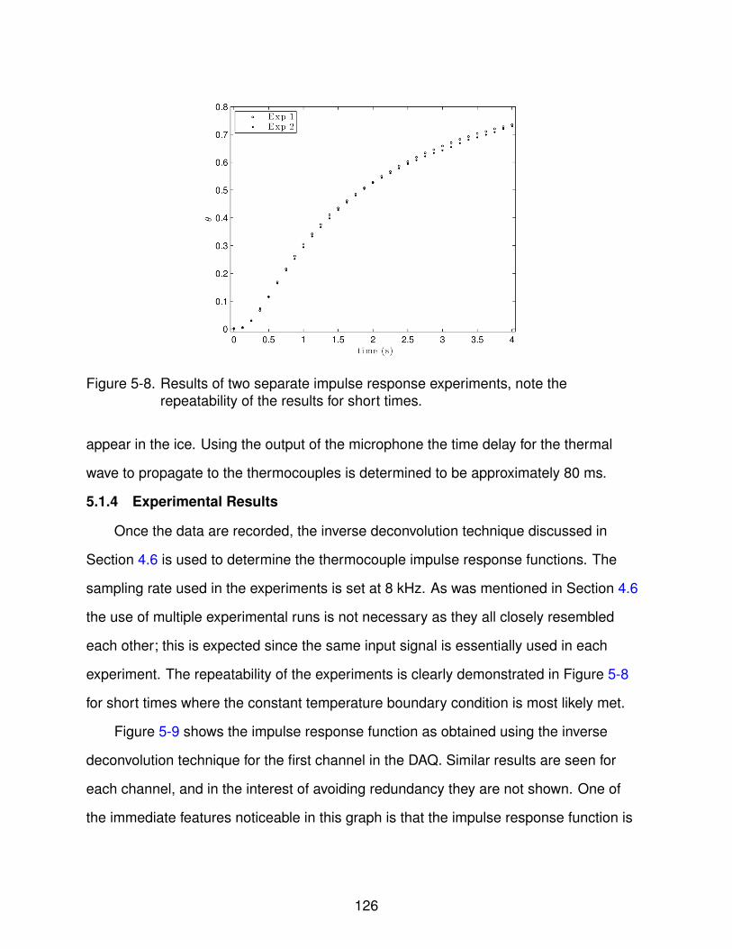
Figure 5-8. Results of two separate impulse response experiments, note therepeatability of the results for short times.

appear in the ice. Using the output of the microphone the time delay for the thermal

wave to propagate to the thermocouples is determined to be approximately 80 ms.

5.1.4 Experimental Results

Once the data are recorded, the inverse deconvolution technique discussed in

Section 4.6 is used to determine the thermocouple impulse response functions. The

sampling rate used in the experiments is set at 8 kHz. As was mentioned in Section 4.6

the use of multiple experimental runs is not necessary as they all closely resembled

each other; this is expected since the same input signal is essentially used in each

experiment. The repeatability of the experiments is clearly demonstrated in Figure 5-8

for short times where the constant temperature boundary condition is most likely met.

Figure 5-9 shows the impulse response function as obtained using the inverse

deconvolution technique for the first channel in the DAQ. Similar results are seen for

each channel, and in the interest of avoiding redundancy they are not shown. One of

the immediate features noticeable in this graph is that the impulse response function is

126

Figure 5-9. Inverse method deconvolution results.

non-zero at the initial time; thus second order and higher impulse response functions

can be ruled out.

5.1.5 Comparison to Established Models

To determine the best impulse response model for the thermocouples, a comparison

is made to a first order response, a 2 exponential response, as well as the model of

Rabin and Rittel. This is accomplished via the use of a nonlinear least squares curve

fit using the function lsqcurvefit available in MatLab, which uses a trust region reflective

algorithm. After the parameters of the model are determined, a comparison of the

output of the impulse response model with the actual temperature measured during

experiments is made; a comparison of the model with the impulse response function

determined via the inverse deconvolution algorithm is also made.

To remain general, the first order system model is modified such that two parameters

are used instead of the single time constant of the rigorous model of Equation (5–3), this

new equation is

h(t) = a exp(−bt). (5–9)

127

Figure 5-10. Comparison of the first order response function to the de-convolvedimpulse response function.

The resulting parameters determined for the first channel of the DAQ are a = 0.532

and b = 0.623; this is equivalent time constant of approximately 1.75 seconds. A

comparison of the resulting function with that produced via the inverse algorithm

is shown in Figure 5-10. It is evident that the behavior of the function is captured

marginally by a first order response. The differences between the response model

output and the experimental data are shown in Figure 5-11. While the overall trend

is captured quite well, there is noticeable error between the predicted and measured

temperature results.

To remain general, the model of Rabin and Rittel is modified as well such that three

parameters are used instead of the two in Equation (5–10). This new equation is

h(t) = c exp(−dtn). (5–10)

The resulting parameters for the first thermocouple channel after deconvolution are c =

1.775, d = 0.216, and n = 0.369 assuming that the radius of the thermocouple is 0.5 mm

and using the thermal diffusivity of copper. A comparison of the resulting function with

128

Figure 5-11. Best fit results using a first order impulse response function.

Figure 5-12. Comparison of the model of [114] to the de-convolved impulse responsefunction.

that produced via the inverse algorithm for the first channel is shown in Figure 5-12. This

model compares well with the inverse method deconvolution. However, there is some

disagreement near t = 0. The differences between the response model output and the

experimental data are shown in Figure 5-13. The trend is captured quite well.

129

Figure 5-13. Best fit results using the model of [114] response function.

Comparison of the parameter d to B in Table 5-1 shows that there is some

departure from the model of Rabin and Rittel as they are of different orders of magnitude.

The value of the exponent, n is of the same order of magnitude. It is noted that the

thermal conductivity ratio for the thermocouple to the copper disc is on the order of 10−2,

well outside the recommended range, and so the comparison is general in nature.

As observed in Figure 5-13 the model of Rabin and Rittel produces good results

despite the differences in the coefficients of the curve fit. There are some conditions

in the experiments that are not accounted for in the model. Namely, there will be some

finite thermal resistance between the thermocouple and the copper disc, although it

is believed to be small due to the use of silver solder in attaching the thermocouples.

Additionally, the thermocouples in the experiments are not fully embedded in the solid,

but they are soldered to the back of the copper disc. This assumption may not be bad

due to the fact that the silver solder will tend to encase the thermocouples.

The final comparison is that of the 2 exponential model. The resulting model

parameters for the first channel of the DAQ are a = 0.658, b = 0.402, c = 0.228, and

130

Figure 5-14. Comparison of the 2 exponential model to the deconvolution algorithmresults.

d = 2.961. A comparison of the resulting function with the results of the deconvolution

algorithm is shown in Figure 5-14; the agreement of the results is excellent. These

results translate into good agreement between the output model and the experimental

data as shown in Figure 5-15.

The results of the comparison of the three models show that the model of Rabin and

Rittel and the 2 exponential model produce the best results. However, the 2 exponential

model is selected as the best due to the fact that excellent agreement is observed

between the curve fitted and deconvolution results.

5.2 Inverse Heat Transfer Algorithm Verification

The purpose of this portion of the current study is to develop an inverse heat

transfer algorithm to determine the heat transfer coefficient of an impinging jet. However,

due to sensitivity issues associated with having sensors placed on the back surface of

the test sample, direct estimation of the surface heat transfer coefficient is difficult, if

not impossible, for high Biot numbers. As such the inverse heat transfer algorithm was

formulated such that the surface temperature is determined and the surface heat flux is

131

Figure 5-15. Best fit results using the 2 exponential model.

then estimated, after which the surface heat transfer coefficient is estimated. In order to

determine the accuracy of the proposed algorithm a parametric study is considered.

5.2.1 Inverse Quenching Parametric Study Setup

There are several different factors which can affect the inverse heat transfer study

which are: the material properties of the disc (i.e. the thermal diffusivity), the impulse

response functions, the height, L, of the disc, the aspect ratio of the disc (L/R), the Biot

number distribution, the number of measurement points on the backside of the disc, and

the magnitude of the noise of the DAQ. Different values for these variables are selected

for the parametric study as detailed below.

The setup for the inverse heat transfer parametric study will simulate the copper

disc assembly outlined in Section 5.1.3. The copper disc is at an initial condition of zero

in dimensionless temperature and then the jet is initiated with a specified Biot number

distribution and an adiabatic wall temperature of unity. The heat transfer coefficient of an

impinging jet can be modeled as a Gaussian function as seen below

132

Bi = Bimax

(1− ratio)

[exp

(−r 2

2σ2

)+ ratio

](5–11)

where Bimax is the maximum Biot number seen, r is the radial coordinate, σ is the

standard deviation which affects the width of the Gaussian peak, and ratio is the ratio of

the maximum to minimum Biot number. Figure 5-16 shows the Biot number distribution

for different values of Bimax , while Figure 5-17 shows the Biot number distribution for

different values of σ, in both figures the value of ratio is 0.1. Three different Bimax values

of 15, 5, and 0.5 were used in the parametric study, these represent peak heat transfer

coefficients of 234, 78, and 7.8 kW/m2 K, respectively. One point of note is that for

higher values of σ the Biot number distribution approaches that of a constant Biot

number, making the problem behave one-dimensional, which is a simpler estimation

problem. This effect is also seen for higher values of the parameter, ratio. To adequately

determine the effectiveness of the inverse heat transfer algorithm the ratio quantity

was set to 0.1 and for most numerical experiments σ was set to 0.1 as well, although

studies at higher values of σ were carried out in order to verify that good results could be

obtained.

The effects of the impulse response function, and the magnitude of the noise

are also explored. While it was found in Section 5.1.5 that the 2 exponential model

produced the best results experimentally, it is difficult to assess the effect of varying

each parameter of the model. As such the first order impulse response function in

Equation (5–3) was chosen to simulate the thermocouple measurement dynamics as

it does a fair job of approximating the dynamics, and it only contains one constant to

vary. The different time constants chosen for the parametric study are 0.1, 1, and 5

seconds which allow for comparison to be made for short and long time delays of the

thermocouples.

To determine the effect of the disc height and aspect ratio on the inverse heat

transfer problem, the maximum radius of the disc, R, was set to 25.4 mm and three

133

Figure 5-16. Biot number distribution showing the effects of Bimax .

different values of the height were selected: 15, 10, and 5 mm giving aspect ratios of

0.591, 0.394, and 0.197, respectively . While performing the parametric study it was

found that for heights of 15 mm, the inverse heat transfer algorithm would not converge;

thus no results from this height are reported in the study. The effect of the disc thermal

diffusivity, the impulse response function, and the height of the disc can be collapsed

into a dimensionless time constant defined below

τ ∗ =τα

L2. (5–12)

To assess the effects of measurement noise, white Gaussian noise was added

to the simulated measurements. The magnitude of the noise in dimensionless space

depends on two separate variables, the initial temperature and the magnitude of the

noise in the DAQ. This relationship is shown below

ε =σDAQTo

(5–13)

134

Figure 5-17. Biot number distribution showing the effects of σ.

where ε is the dimensionless noise, σDAQ is the standard deviation of the measurement

noise of the DAQ, and To is the initial temperature. The initial temperature was set

to 150 C and two different standard deviations of the DAQ were chosen: 0.2 C, the

measurement noise seen in the DAQ used for determining the impulse response

function, and 1 C.

In addition to the above conditions, other conditions were set for the parametric

study. The sampling frequency was set to 8 kHz and the grid resolution was set to 32

by 32 for L = 10mm. Oscillations of heat flux similar to the ones seen in Section 4.5.3

were present in the L = 5 mm case and were eliminated by using a grid resolution of

64 by 64. The total time duration of the simulated experiments was set to 30,000 time

steps, 25,000 of which were used in the stopping criteria, except for the Bimax = 0.5, L

= 5 mm simulations where 60,000 time steps were used, 50,000 of which were used in

the stopping criteria. The reason for this disparity is that the lower Biot number caused

a slower response in the measured temperature. Additionally, the number of simulated

135

measurements taken was selected to be 8 and 16, the measurement locations were

defined by the following formula

ri ,meas = R

(i

pts− 1

2pts

)i = 1, 2, 3, ...M (5–14)

where ri ,meas is the location of measurement i, R is the radius of the disc, pts is the

number of measurement points, and M is the total number of measurements.

5.2.2 Error Assessment Methods

In order to quantify the error between the inverse heat transfer algorithm results

and the true Biot number an error definition must be made. The algorithm is technically

designed to estimate the surface temperature and thus a surface temperature error

should be used to estimate the effectiveness. Additionally, because the Biot number is

the quantity of interest it must be estimated as well. The error assessment chosen is

that of a root-mean-square error, the rms error equation for the surface temperature and

Biot number distribution is defined below

eξ,rms =

√∫t∗

∫r∗

(ξact − ξinv)2 r ∗dr ∗dt∗√∫t∗

∫r∗

(ξact)2 r ∗dr ∗dt∗

. (5–15)

where ξ is either the dimensionless surface temperature or Biot number, the subscript

act denotes the input variable, and the subscript inv denotes the output variable returned

by the inverse method.

While performing the parametric study it was found that the estimation of the Biot

number near t∗ = 0 was grossly in error, being several orders of magnitude greater than

the actual Biot number. The large Biot numbers near the initial time are not believable.

However, after this initial spike, the Biot number estimated will generally maintain a near

constant value for a portion of the results and it was decided that the Biot number rms

error would be assessed such that only this portion of the Biot number distribution would

be used in the error calculations, this is shown in Figure 5-18.

136

Figure 5-18. Comparison of the inverse results of Biot number at the centerline of thedisc for Bimax = 15, τ = 0.1. The asterisks denote where the results aretruncated.

Additionally, because of the near constant Biot number after the initial time it was

decided that the Biot number would be averaged temporally between the truncation

points. This average Biot number, denoted as Biave , was also used to determine an rms

error as defined below

eBiave ,rms =

√∫r∗

(Biave,real − Biave,inv)2 r ∗dr ∗√∫

r∗(Biave,real)

2 r ∗dr ∗. (5–16)

5.2.3 Parametric Study Results

The results for the parametric study for L = 10 mm and σDAQ = 0.2 C are listed in

Table 5-2. It is clearly evident that the inverse method accurately determines the surface

temperature distribution, which it is designed to do. The accuracy ranges from 1 to 3

% and does not seem to be affected by increasing the number of measurement points.

The truncated Biot number error is noticeably higher, ranging from 15 to 48 % for the 8

137

Table 5-2. RMS errors for L = 10 mm, and σDAQ = 0.2 C.eθs ,rms eBi ,rms (truncated) eBiave ,rmsτ ∗ τ ∗ τ ∗

0.112 1.123 5.617 0.112 1.123 5.617 0.112 1.123 5.617

M = 815 0.012 0.018 0.018 0.153 0.167 0.176 0.139 0.153 0.162

Bimax 5 0.013 0.017 0.019 0.261 0.304 0.380 0.251 0.293 0.3410.5 0.015 0.007 0.014 0.429 0.396 0.475 0.330 0.365 0.424

M = 1615 0.012 0.016 0.020 0.137 0.151 0.303 0.129 0.088 0.258

Bimax 5 0.016 0.017 0.025 0.312 0.295 0.374 0.309 0.277 0.3440.5 0.018 0.010 0.017 0.497 0.608 0.716 0.442 0.594 0.654

measurement points case; the error tends to increase for a lower Bimax . Contour plots

of the errors for the L = 10 mm, σDAQ = 0.2 C, and 8 measurement points are shown in

Figure 5-19; in the interest of neatness contour plots of the other cases are not shown in

this Chapter and can be found in Appendix B. For 16 measurement points, the error is

in the same range for the two highest Bimax cases, but is noticeably higher for the lowest

case. The error for the temporally averaged Biot number error is slightly lower than that

of the truncated Biot number error for both 8 and 16 measurement points. From these

data it appears that for L = 10 mm, increasing the measurement points beyond 8 has

only an marginal increase in the accuracy of the inverse method for these conditions.

Data for the L = 10 mm, σDAQ = 1 C, and 8 measurement points is found in

Table 5-3. The magnitude for all three errors is near the same range as that found for the

σDAQ = 0.2 C case; thus the inverse method is insensitive to noise of approximately 0.7

%. Simulations for 16 measurement points were not performed for this case due to the

results seen for σDAQ = 0.2 C.

The error results for L = 5 mm and σDAQ = 0.2 C is found in Table 5-4. It is seen

that the surface temperature error for both 8 and 16 measurement points is very low, 1

% or less. However, the error for Bimax = 0.5 is an order of magnitude greater than the

error found for the other two cases. The error for the truncated Biot number distribution

138

a b

c

Figure 5-19. Error Contours for L = 10 mm, σDAQ = 0.2 C, and 8 measurement points.a) eBiave ,rms , b) eBi ,rms (truncated), and c) eθs ,rms .

Table 5-3. RMS errors for L = 10 mm, σDAQ = 1 C, and M = 8.eθs ,rms eBi ,rms (truncated) eBiave ,rmsτ ∗ τ ∗ τ ∗

0.112 1.123 5.617 0.112 1.123 5.617 0.112 1.123 5.617

15 0.017 0.022 0.015 0.204 0.253 0.223 0.166 0.165 0.173Bimax 5 0.017 0.017 0.019 0.341 0.302 0.371 0.328 0.287 0.327

0.5 0.012 0.012 0.015 0.502 0.697 0.529 0.408 0.328 0.475

with 8 measurement points ranges from 10 to 30 % for maximum Biot numbers of

5 and 15, but the error is very much increased for the Bimax = 0.5 case, essentially

demonstrating that the estimated Biot number distribution is useless. The truncated

139

Table 5-4. RMS errors for L = 5 mm and σDAQ = 0.2 C.eθs ,rms eBi ,rms (truncated) eBiave ,rmsτ ∗ τ ∗ τ ∗

0.449 4.493 22.47 0.449 4.493 22.47 0.449 4.493 22.47

M = 815 0.003 0.007 0.011 0.143 0.094 0.316 0.022 0.052 0.108

Bimax 5 0.003 0.005 0.006 0.166 0.156 0.121 0.030 0.060 0.0510.5 0.012 0.011 0.014 1.381 1.006 1.071 1.114 0.960 0.984

M = 1615 0.002 0.007 0.010 0.170 0.133 0.234 0.030 0.036 0.136

Bimax 5 0.002 0.004 0.006 0.103 0.100 0.158 0.021 0.039 0.0940.5 0.005 0.006 0.009 0.334 0.208 0.291 0.174 0.144 0.190

Table 5-5. RMS error for L = 10 mm,σDAQ = 0.2 C, M = 8, and various values of σ for theBiot number distribution.

Bimax σBi τ ∗ eθs ,rms eBi ,rms eBiave ,rms(truncated)

15 0.25 5.62 0.018 0.130 0.0395 0.25 5.62 0.015 0.070 0.0235 0.5 5.62 0.019 0.056 0.0215 0.75 5.62 0.021 0.090 0.033

Biot number results for 16 measurement points show an error range of 10 to 33 %

for the entire range of maximum Biot numbers, indicating that for low Biot number

distributions an increase in the number of measurement points is warranted. The

temporally averaged Biot number error shows similar trends, as expected.

Table 5-5 shows error results for the Biot number distribution with σ 6= 0.1. The

magnitude of the error for surface temperature is similar to that seen in the σ = 0.1 case.

However, the truncated Biot number and temporally averaged Biot number show a large

increase in accuracy. The reason for this change was mentioned previously. With a

larger value of σ the problem behaves more like a one-dimensional estimation problem,

which less complex.

When determining the impulse response functions for thermocouples there is

a potential for error between the real impulse response function of the sensor and

140

Table 5-6. RMS error for L = 10 mm and M = 8 with different actual and simulated timeconstants.

Bimax σBi τ ∗act τ ∗sim eθs ,rms eBi ,rms eBiave ,rms(truncated)

15 0.1 0.112 0.107 0.012 0.148 0.13315 0.1 0.112 0.118 0.012 0.147 0.12915 0.1 1.123 1.011 0.047 0.290 0.26215 0.1 1.123 1.067 0.037 0.241 0.20715 0.1 5.617 5.055 0.079 0.599 0.56815 0.1 5.617 5.505 0.026 0.393 0.34615 0.25 5.617 5.505 0.052 0.504 0.42615 0.25 5.617 5.729 0.045 0.202 0.1355 0.1 1.123 1.180 0.041 0.504 0.4735 0.1 1.123 1.067 0.040 0.475 0.459

the results of experiments. These errors can be produced due to not being able to

accurately determine when the experiment was initiated, or errors due to the boundary

condition on the top surface not being precisely known. To determine the affect these

errors have on determining the Biot number distribution, simulations were carried

out such that the time constant for the inverse algorithm (τ ∗sim) would be different than

the actual time constant for the sensors (τ ∗act). This study was restricted to the L = 10

mm, σDAQ = 0.2 C case, and the errors simulated ranged from 1 to 10 %. The results

from this study can be found in Table 5-6. It is noticed that for small time constants,

the difference is not very noticeable. However, as the magnitude of the time constant

increases, so does the the magnitude of the error. For a time constant of 5 seconds the

results are essentially unusable. Clearly care must be taken to ensure that the impulse

response functions are estimated accurately, especially when the time constants are

large.

5.2.4 Heat Loss/Gain Effects

When performing a transient jet impingement heat transfer experiment the effects of

non-ideal insulation will be present, as briefly discussed in Section 5.1.3. These effects

will cause the disc to gain heat from the insulation after the jet is initiated, with more

141

heat entering on the bottom near the maximum radial distance due to there being more

insulation touching the disc in that area. While this heat gain is very low in magnitude

and causes on a slight error (approximately 3 % at t = 1 second) it will tend to have

a larger impact on the determination of the surface temperature and hence heat flux

and Biot number. These effects have been demonstrated by simulating the disc being

at an initial dimensionless temperature of zero and having a surface temperature of

unity being applied to it and recording the temperature at 8 locations on the back side

of the disc; this simulation includes the ceramic insulation and allows heat exchange

between it and the copper disc. The simulated measurements are then input into first

order impulse response model,and white Gaussian noise of 0.2 C (the dimensional

initial temperature is 150 C) is added. These data are then input into an inverse heat

transfer algorithm which assumes ideal insulation.

The error results for the surface temperature are 0.050, 0.044, and 0.047 for time

constants of 0.1, 1, and 5 seconds, respectively. While this error is small the real effect

lies in the estimation of the heat flux, which has a non-uniform distribution. Figure 5-20

shows the difference between the inverse and exact solutions. Clearly the error will

produce noticeable error in the calculation of Biot number.

5.2.5 Effectiveness of the Inverse Heat Transfer Algorithm

All of the major factors affecting the inverse heat transfer have been explored and

quantified. From the results it is seen that for times near t = 0 there is significant error in

the returned surface temperature which is carried over in the determination of surface

heat flux and Biot number. This shows that the developed heat transfer algorithm will not

be effective at detecting phase change heat transfer near the initial instant in time, where

it is most likely to occur, without modification. A possible method to overcome some of

these problems would be to insert the thermocouples into the the disc and have them

located closer to the top surface. However, care must be taken to ensure that any effects

of the thermocouple insertion are either minimized or are explicitly taken into account in

142

Figure 5-20. Comparison of the results between exact solution and inverse results forthe surface heat flux due to a step change in surface temperature. Time =0.375 seconds, τ = 1 second.

the inverse heat transfer algorithm. When the thermocouples are located closer to the

top surface then the problem can also be formulated in terms of an unknown surface

heat flux, which will provide a more accurate estimate of the surface heat flux, and both

inverse problems can be solved. The Biot number can then be determined using this

more accurate information.

The effects due to errors in the estimated impulse response function were explored

and it is imperative that they be determined accurately, especially if the time constant

of the system is above 1 second or else gross error will engulf the results. The effects

due to the magnitude of the noise present were found to be negligible for magnitudes

approximating those found in a laboratory setting. The number of sensors does not

seem to be a contributing factor unless the disc is very thin (has a small L/R ratio). The

time constant of the measurement system does not have a major effect on the accuracy

of the method unless it has some error in its estimate.

143

Figure 5-21. Centerline NuD for Z/D = 6.0 and ReD = 7.25 × 105 as returned from theinverse heat transfer algorithm.

Measurements for the supersonic impinging jet facility were taken and an attempt

was made to determine the Biot number distribution. Figure 5-21 shows results for the

centerline NuD with Z/D = 6.0 and ReD = 7.25 × 105, Figure 5-22 shows the spatial

distribution of NuD for the same experiment, notice that due to the heat gained from

insulation along the side of the disc causes a large overshoot near r∗ =1. Similar results

were found in all experiments performed and the estimates of Nusselt number are

grossly in error.

5.3 Summary

In this Chapter the thermocouple dynamics were investigated. Four separate

models for the measurement dynamics were explored: first order, second order, Rabin

and Rittel, and the two exponential model were introduced. An experimental setup

to determine the proper impulse response model was conducted and the model of

Rabin and Rittel and the two exponential order model produced excellent results by

comparing well between the theoretical output and the experimental measurement. The

144

Figure 5-22. Spatial distribution of NuD for Z/D = 6.0, ReD = 7.25 × 105, and t∗ = 2.11 asreturned from the inverse heat transfer algorithm.

two exponential order model was chosen as the best model do its agreement with the

impulse response function as determined by the inverse deconvolution method.

A parametric study of the inverse method was conducted to explore the effects

of: disc height, the impulse response function, the magnitude and shape of the Biot

number distribution, the number of temperature sensors used, and the magnitude

of the noise from the data acquisition system. The error was assessed using the

root-mean-square error of the surface temperature distribution as well as a truncated

Biot number distribution and a temporally averaged Biot number. It was found that

increasing the number of thermocouples for a disc height of 10 mm had little influence

on the accuracy of the algorithm. For a disc height of 5 mm it was seen that increasing

the number of thermocouples would decrease the error of the inverse method. However,

estimating Biot number distribution with a small magnitude proved to have significant

error.

The relative slowness of the sensor dynamics, characterized by a time constant,

did not seem to have an effect on the accuracy of the inverse algorithm. However, it was

145

seen that for slow response times, a small amount of error in the time constant estimate

will produce large errors in the Biot number distribution. This effect was not present in

the case of small time constants, it was seen to have a negligible effect. The effect of the

data acquisition system noise had no effect at magnitudes experienced in a laboratory

setting.

The effects of heat gain on the inverse problem were explored. It was found that

although the error in the surface temperature estimate was low (approxiamtely 5 %) the

error in the subsequent surface heat flux calculation was very noticeable. Measurements

performed on the supersonic jet impingement facility were unable to produce reliable

estimates of the Biot number distribution.

146

CHAPTER 6CONCLUSIONS

A multi-phase supersonic impinging jet facility for thermal management has been

constructed. The facility operates by taking high pressure air and reducing it to a

pressure between 1.0 and 2.4 MPa where it acts on top of a water storage tank and

passes through a mass flow meter and a mixing chamber. Differential pressure between

the top of the water storage tank and the mixing chamber forces the water through

a regulating orifice where it becomes mixed with the air in the mixing chamber; the

resulting mixture is then expanded through a converging-diverging nozzle, with a design

Mach number of 3.24. It is then directed to a surface where it impinges and removes

heat. The facility sub-systems include: air storage, water storage and flow control,

air pressure control, air mass flow measuring, converging-diverging nozzle, and data

acquisition. Temperature, pressure, and Mach number were calculated throughout

the facility using one-dimensional gas dynamic relations. It was found that at normal

operating conditions no shock wave would be present in the converging-diverging nozzle

and thus the exiting air/liquid mixture is at supersonic speeds. However, because the

operational supply pressure is lower than ideal, the nozzle operates in an overexpanded

manner.

Steady state heat transfer measurements were performed for the impinging

jet facility. These experiments were performed by allowing the jet to impinge on

a nichrome strip with current passing through it and thermocouples recording the

back wall temperatures. The data were then time averaged to eliminate noise and

turbulent fluctuations. Both single-phase and multi-phase experiments were performed

in order to assess the heat removal capabilities of the multi-phase jet and to quantify

heat transfer enhancement with the addition of the small amount of dispersed liquid

droplets. Once the droplets impinge on the surface, a thin liquid film forms on top of the

surface. The heat transfer characteristics of the jet are different near the impingement

147

zone, where droplet impact dominates. Away from the impingement zone, thin film

dynamics dominate the heat transfer process. The peak heat transfer coefficients for

the multi-phase jet exceed 200,000 W/m2-K near the centerline, matching some of

the highest heat transfer rates reported in the literature, while simultaneously having

a significantly reduced liquid flow rate. This reduced flow rate can be advantageous in

some industrial settings.

It was found that increasing the Reynolds number of the jet and the liquid mass

fraction of water increases the Nusselt number of the jet near the centerline. These

effects are diminished far removed from the impingement zone. Nozzle height is seen

to have a slight effect of the Nusselt number near the interior of the jet, but no definite

trend is apparent, and is seen to have no significant impact away form the centerline.

The single phase impinging jet Nusselt numbers compare well with data in the literature.

Comparison between the single and multi-phase jets shows that the addition of the liquid

droplets to the jet enhances heat transfer by an order of magnitude in the interior of the

jet and by a factor of two to five away form the centerline.

There is no evidence of significant phase change heat transfer occurring during the

jet impingement studies. Analysis of the saturated humidity ratio near the centerline of

the jet shows that little evaporation is possible and its effects are essentially negligible.

Determination of the humidity ratio far removed form the centerline of the jet is not

possible due to the lack of information regarding the surface temperature of the film.

However, the Nusselt number in this region remains essentially constant; significant

evaporation would result in increased Nusselt number in this region. The lack of this type

of trend supports the contention that there is no significant phase change heat transfer

taking place. The use of droplet impact theory suggests that heat transfer enhancement

in the jet interior due to phase change may not be possible. The saturation pressure

is significantly elevated due to the high impact velocity of the droplets and will exceed

the critical pressure for the nominal exit velocity of the nozzle. Thus any phase change

148

occurring would not result in additional heat removal as the latent heat of vaporization

above the critical pressure is zero.

An inverse heat transfer algorithm using the conjugate gradient method with adjoint

problem was developed which can determine the Nusselt number for an impinging

jet. This method explicitly takes into account sensor dynamics, a feature that is not

present in inverse methods found in the literature. A procedure to determine the impulse

response function of thermocouples attached to the surface of a solid was developed

using ice to cause a step change in surface temperature. The resulting data is then

input into a deconvolution algorithm which returns the impulse response function via an

inverse method. This allows insight into the underlying functional form and allows the

proper impulse response function model to be found. Four different impulse response

function models were explored: a first order model, a second order model, the model

of Rabin and Rittel, and the two exponential model. It was found that the model of

Rabin and Rittel and the two exponential model produced the best agreement when

compared to experimental results. However, due to the fact that the two exponential

model produced better agreement between the impulse response functions determined

via curve-fit and inverse algorithm, it was chosen as the best model for the surface

mounted thermocouples used in those experiments.

A parametric study was performed using simulated data to explore the effects of the

disc height and aspect ratio, the magnitude and shape of the Biot number distribution,

the number of sensors used, the impulse response function, and the magnitude of

the noise of the data acquisition system on the error associated with the IHT method.

To assess the error in the inverse heat transfer algorithm three different errors were

considered, the rms error between input surface temperature and that returned by the

inverse method, the rms error between the input Biot number and that returned by the

inverse method during a truncated time domain when the behavior of the returned Biot

number was nearly constant, and the rms error between the input Biot number and the

149

temporally average Biot number over the same truncated time domain. The inverse heat

transfer algorithm is specifically designed to estimate the surface temperature and as

such the error in its estimate was very small, on the order of a few percent. The error

for estimating Biot number was noticeably higher, ranging from 10 % to over 80 % in

some cases. Most of the factors investigated appear to have little effect on the inverse

heat transfer method. However, the magnitude of the Biot number distribution had a

large effect. A lower Biot number produces small changes in measured temperature and

thus is a difficult estimation problem and any error in the surface temperature estimation

is carried over and amplified in the surface heat flux calculation. Errors in the impulse

response function were seen to have a large effect in certain cases. If the overall delay

in the impulse response function is short, then the method can tolerate some error.

However, if the overall delay is as high as 5 seconds, then even an error as small as one

percent can render the results of the inverse heat transfer algorithm useless.

Finally the effects of heat loss/gain from insulation on the impingement target

were investigated. The difference in temperature at the simulated measurement points

between an idealized disc and one with heat transfer to/from its insulation was small,

approximately 3 %. However, this small error is magnified by the inverse algorithm,

causing it to overestimate the heat flux near the edge of the disc. These finding were

verified by performing experiments using the multi-phase jet impingement facility.

In order for the inverse method to be effective, the heat exchange with the

insulation must be taken into account. The effects of the heat exchange could also

be lessened by locating the temperature sensors closer to the top surface. However,

inserting thermocouples inside of the disc is likely to distort the heat flow and so some

compromise must be made.

150

APPENDIX ACOMPLETE STEADY STATE TWO-PHASE HEAT TRANSFER JET RESULTS

There are many heat transfer data sets for the steady state experiments discussed

in Chapter 3 which are not presented due to space considerations and because all of

the results follow the trends discussed therein. For the sake of completeness, the heat

transfer results for the steady state two-phase impinging jet results are presented in this

Appendix.

For Figures A-1 through A-3 the same orifice is used for each experiment, thus

keeping the water mass fraction nominally constant. Jet Reynolds number is held

constant as well, and the nozzle spacing is varied.

For Figures A-4 through A-7 the nozzle spacing and Reynolds number are constant.

The orifice is changed to vary water mass fraction.

For Figures A-8 through A-10 the same orifice is used for each experiment, thus

keeping the water mass fraction and jet Reynolds number nominally constant, and the

nozzle spacing is varied.

For Figures A-11 through A-14 the nozzle spacing and Reynolds number are

constant, and the orifice is changed to vary water mass fraction.

151

a b

c d

Figure A-1. Two-phase NuD results for various nozzle height to diameter ratios. a) w =0.0205, ReD = 4.54 × 105, b) w = 0.0240, ReD = 4.47 × 105, c) w = 0.0357,ReD = 4.42 × 105, and d) w = 0.0375, ReD = 4.42 × 105

152

a b

c d


153

a b

c d


154

a

b

c

Figure A-4. Two-phase NuD results for various liquid mass fractions and Z/D = 2.0. a)ReD = 4.42 × 105, b) ReD = 7.20 × 105, and c) ReD = 1.01 × 106

155

a

b

c


156

a

b

c


157

a

b

c


158

a b

c d

Figure A-8. Two-phase enhancement ratio results for various nozzle height to diameterratios. a) w = 0.0205, ReD = 4.54 × 105, b) w = 0.0240, ReD = 4.47 × 105,c) w = 0.0357, ReD = 4.42 × 105, and d) w = 0.0375, ReD = 4.42 × 105

159

a b

c d


160

a b

c d


161

a

b

c

Figure A-11. Two-phase enhancement results for various liquid mass fractions and Z/D= 2.0. a) ReD = 4.42 × 105, b) ReD = 7.20 × 105, and c) ReD = 1.01 × 106

162

a

b

c

Figure A-12. Two-phase enhancement ratio results for various liquid mass fractions andZ/D = 4.0. a) ReD = 4.43 × 105, b) ReD = 7.35 × 105, and c) ReD = 1.03 ×106

163

a

b

c


164

a

b

c


165

APPENDIX BCOMPLETE INVERSE HEAT TRANSFER ALGORITHM ERROR ASSESSMENT

CONTOUR PLOTS

There are many data sets for the three different errors used to assess the

effectiveness of the inverse heat transfer algorithm and as such all of them were

not included in Chapter 5. In the interest of completeness they are included in this

Appendix. Figure B-1 shows the error contours for the L = 5 mm, σDAQ = 0.2 C, and 8

measurement points case. Figure B-2 shows the error contours for the L = 5 mm, σDAQ =

0.2 C, and 16 measurement points case. Figure B-3 shows the error contours for the L

= 10 mm, σDAQ = 0.2 C, and 8 measurement points case. Lastly, Figure B-5 shows the

error contours for the L = 10 mm, σDAQ = 1 C, and 8 measurement points case.

166

a

b

c

Figure B-1. Error Contours for L = 5 mm, σDAQ = 0.2 C, and 8 measurement points. a)eBiave ,rms , b) eBi ,rms (truncated), and c) eθs ,rms

167

a

b

c


168

a

b

c


169

a

b

c

Figure B-4. Error Contours for L = 10 mm, σDAQ = 0.2 C, and 16 measurement points.a) eBiave ,rms , b) eBi ,rms (truncated), and c) eθs ,rms

170

a

b

c

Figure B-5. Error Contours for L = 10 mm, σDAQ = 1 C, and 8 measurement points. a)eBiave ,rms , b) eBi ,rms (truncated), and c) eθs ,rms

171

APPENDIX CIMAGES OF ORIFICES USED DURING EXPERIMENTS

During operation of the jet facility it was noticed that the 0.38 mm orifice provided

a lower liquid flowrate than the 0.33 mm orifice. After examining the different orifices

under an optical microscope it was discovered that the 0.38 and 0.51 mm orifices were

not perfectly circular. This eccentricity is very noticeable in the 0.38 mm orifice and

may result in different spray characteristics, which could have affected the heat transfer

results. The eccentricity is not as severe in the 0.51 mm orifice and did not seem to

affect the heat transfer results. Figures C-1 through C-4 show images of the orifices

under 4X magnification.

Figure C-1. The 0.33 mm orifice.

172

Figure C-2. The 0.37 mm orifice, note the high degree of eccentricity in the orifice

Figure C-3. The 0.41 mm orifice.

173

Figure C-4. The 0.51 mm orifice, note the eccentricity in the orifice

174

REFERENCES

[1] X. Liu, J. H. Lienhard V, Extremely High Heat Fluxes beneath Impinging LiquidJets, Journal of Heat Transfer 115 (1993) 472–476.

[2] C. H. Oh, J. H. Lienhard V, H. F. Younis, R. S. Dahbura, D. Michels, LiquidJet-Array Cooling Modules for High Heat Fluxes, AIChE Journal 44 (1998)769–779.

[3] J. H. Lienhard V, J. Hadeler, High Heat Flux Cooling by Liquid Jet Array Modules,Chemical Engineering and Technology 22 (1999) 867–970.

[4] J. F. Klausner, R. Mei, S. Near, R. Stith, Two-Phase Jet Impingement forNon-Volatile Residue Removal, Proceedings of the I MECH E Part E Journalof Process Mechanical Engineering 212 (1998) 271–279.

[5] K. Hiemenz, Die Grenzschicht an Einem in den Gleichformigen FlussigkeitsstromEingetauchten Geraden Kreiszylinder, Dinglers polytechnisches Journal 326(1911) 321–324.

[6] F. Homann, Der einfluss grosser zahigkeit bei der stromung um den zylinder undum die kugel, Zeitschrift fur Angewandte Mathematik und Mechanik 16 (1936)153–164.

[7] C. Y. Wang, Stagnation flows with Slip: Exact Solutions of the Navier-StokesEquations, Zeitschrift fr Angewandte Mathematik und Physik (ZAMP) 54 (2003)184–189. 10.1007/PL00012632.

[8] H. Schlichting, K. Gersten, Boundary Layer Theory, Springer, 8th edition, 2000.

[9] A. A. Kendoush, Theory of Stagnation Region Heat and Mass Transfer to FluidJets Impinging Normally on Solid Surfaces, Chemical Engineering and Processing37 (1998) 223 – 228.

[10] X. Liu, J. H. Lienhard V, Liquid Jet Impingement Heat Transfer on a Uniform FluxSurface, Heat Transfer Phenomena in Radiation, Combustion and Fires ASMEHTD 106 (1989) 523–530.

[11] X. Liu, J. H. Lienhard V, J. S. Lombara, Convective Heat Transfer by Impingementof Circular Liquid Jets, Journal of Heat Transfer 113 (1991) 571–582.

[12] X. Wang, Z. Dagan, L. Jiji, Heat Transfer between a Circular Free Impinging Jetand a Solid Surface with Non-Uniform Wall Temperature or Wall Heat Flux–1.Solution for the Stagnation Region, International Journal of Heat and MassTransfer 32 (1989) 1351 – 1360.

[13] X. Wang, Z. Dagan, L. Jiji, Heat Transfer between a Circular Free Impinging Jetand a Solid Surface with Non-Uniform Wall Temperature or Wall Heat Flux–2.

175

Solution for the Boundary Layer Region, International Journal of Heat and MassTransfer 32 (1989) 1361 – 1371.

[14] X. S. Wang, Z. Dagan, L. M. Jiji, Conjugate Heat Transfer Between a LaminarImpinging Liquid Jet and a Solid Disk, International Journal of Heat and MassTransfer 32 (1989) 2189 – 2197.

[15] D. H. Lee, J. Song, M. C. Jo, The Effects of Nozzle Diameter on Impinging JetHeat Transfer and Fluid Flow, Journal of Heat Transfer 126 (2004) 554–557.

[16] J. Baonga, H. Louahlia-Gualous, M. Imbert, Experimental Study of theHydrodynamic and Heat Transfer of Free Liquid Jet Impinging a Flat CircularHeated Disk, Applied Thermal Engineering 26 (2006) 1125 – 1138.

[17] J. H. Lienhard V, X. Liu, L. A. Gabour, Splattering and heat Transfer duringImpingement of a Turbulent Liquid Jet, Journal of Heat Transfer 114 (1992)362–372.

[18] D. E. Hall, F. P. Incropera, R. Viskanta, Jet Impingement Boiling from a CircularFree-Surface Jet During Quenching: Part 1—Single-Phase Jet, Journal of HeatTransfer 123 (2001) 901–910.

[19] K. Jambunathan, E. Lai, M. Moss, B. Button, A Review of Heat Transfer Data forSingle Circular Jet Impingement, International Journal of Heat and Fluid Flow 13(1992) 106 – 115.

[20] D. Michels, J. Hadeler, J. H. Lienhard, High-Heat-Flux Resistance Heatersfrom VPS and HVOF Thermal Spraying, Experimental Heat Transfer 11 (1998)341–359.

[21] J. H. Lienhard V, D. Napolitano, Thermal Stress Limits of Plates Subjected toExtremely High Heat Flux, Proceedings of the ASME Heat Transfer DivisionVolume 2 ASME HTD-Volume 333 (1996) 23–35.

[22] J. H. Lienhard V, Annual Review of Heat Transfer, Begell House, pp. 199–270.

[23] B. Webb, C.-F. Ma, Advances in Heat Transfer, volume 26, Elsevier, pp. 105 – 217.

[24] H. Martin, Advances in Heat Transfer, volume 13, Elsevier, pp. 1–60.

[25] I. A. Kopchikov, G. I. Voronin, T. A. Kolach, D. A. Labuntsov, P. D. Lebedev, LiquidBoiling in a Thin Film, International Journal of Heat and Mass Transfer 12 (1969)791–796.

[26] K. A. Estes, I. Mudawar, Correlation of Sauter Mean Diameter and Critical HeatFlux for Spray Cooling of Small Surfaces, International Journal of Heat and MassTransfer 38 (1995) 2985 – 2996.

176

[27] K. M. Graham, S. Ramadhyani, Experimental and Theoretical Studies of Mist JetImpingement Cooling, Journal of Heat Transfer 118 (1996) 343–349.

[28] L. Bolle, J. Moureau, Spray Cooling of Hot Surfaces, Mulitphase Science andTechnology 1 (1982) 1–97.

[29] V. I. Zapryagaev, A. N. Kudryavtsev, A. V. Lokotoko, A. V. Solotchin, A. A. Pavlov,H. A., An Experimental and Numerical Study of a Supersonic-Jet Shock-WaveStructure, in: Proceedings of West East High Speed Flow Fields: AerospaceApplications from High Subsonic to Hypersonic Regime, Marseilles, France, pp.346–351.

[30] C. d. Donaldson, R. S. Snedeker, A Study of Free Jet Impingement. Part 1. MeanProperties of Free and Impinging Jets, Journal of Fluid Mechanics 45 (1971)281–319.

[31] D. C. Pack, On the Formation of Shock-Waves in Supersonic Gas Jets, TheQuarterly Journal of Mechanics and Applied Mathematics 1 (1948) 1–17.

[32] D. C. Pack, The Reflexion and Diffraction of Shock Waves, Journal of FluidMechanics 18 (1964) 549–576.

[33] C.-W. Chu, Compatibility Relations and a Generalized Finite-DifferenceApproximation for Three-Dimensional Steady Supersonic Flow, AIAA Journal5 (1967) 493–501.

[34] J. H. Gummer, B. L. Hunt, The Impingement of a Uniform, Axisymmetric,Supersonic Jet on a Perpendicular Flat Plate, Aeronautical Quarterly 22 (1971)403–420.

[35] J. C. Carling, B. L. Hunt, The Near Wall Jet of a Normally Impinging, Uniform,Axisymmetric, Supersonic Jet, Journal of Fluid Mechanics 66 (1974) 159–176.

[36] A. Powell, On the Mechanism of Choked Jet Noise, Proceedings of the PhysicalSociety. Section B 66 (1953) 1039.

[37] A. Powell, On Edge Tones and Associated Phenomena, Acoustica 3 (1953)233–243.

[38] C. K. W. Tam, K. K. Ahuja, Theoretical Model of Discrete Tone Generation byImpinging Jets, Journal of Fluid Mechanics 214 (1990) 67–87.

[39] A. Krothapalli, Discrete Tones Generated by an Impinging UnderexpandedRectangular Jet, AIAA Journal 23 (1985) 1910–1915.

[40] F. S. Alvi, W. W. Bower, J. A. Ladd, Experimental and Computational Investigationof Supersonic Impinging Jets, AIAA Journal 40 (2002) 599–609.

177

[41] K. Klinkov, A. Erdi-Betchi, M. Rein, Behavior of Supersonic OverexpandedJets Impinging on Plates, in: H.-J. Rath, C. Holze, H.-J. Heinemann, R. Henke,H. Hnlinger (Eds.), New Results in Numerical and Experimental Fluid MechanicsV, volume 92 of Notes on Numerical Fluid Mechanics and Multidisciplinary Design,Springer Berlin / Heidelberg, 2006, pp. 168–175.

[42] S.-c. Baek, S.-B. Kwon, Study of Moderately Underexpanded Supersonic MoistAir Jets, AIAA Journal 44 (2006) 1624–1627.

[43] M. M. Ashraful Alam, S. Matsuo, T. Setoguchi, Effect of Non-EquilibriumHomogeneous Condensation on the Self-Induced Flow Oscillation of SupersonicImpinging Jets, International Journal of Thermal Sciences 49 (2010) 2078 – 2092.

[44] M. M. Ashraful Alam, S. Matsuo, T. Setoguchi, Supersonic Moist Air JetImpingements on Flat Surface, Journal of Thermal Science 19 (2010) 51–59.10.1007/s11630-010-0051-3.

[45] Y. Otobe, S. Matsuo, M. Tanaka, H. Kashimura, H.-D. Kim, T. Setoguchi, A studyof under-Expanded Moist Air Jet Impinging on a Flat Plate, Journal of ThermalScience 14 (2005) 334–340. 10.1007/s11630-005-0054-7.

[46] C. D. Donaldson, R. S. Snedeker, D. P. Margolis, A Study of Free JetImpingement. Part 2. Free Jet Turbulent Structure and Impingement Heat Transfer,Journal of Fluid Mechanics 45 (1971) 477–512.

[47] M. D. Fox, M. Kurosaka, Supersonic Cooling by Shock-Vortex Interaction, Journalof Fluid Mechanics 308 (1996) 363–379.

[48] B. G. Kim, M. S. Yu, Y. I. Cho, H. H. Cho, Distributions of Recovery Temperatureon Flat Plate by Underexpanded Supersonic Impinging Jet, Journal ofThermophysics and Heat Transfer 16 (2002) 425–431.

[49] H. W. Liepmann, A. Roshko, Elements of Gasdynamics, John Wiley & Sons Inc,1957.

[50] J. E. John, T. G. Keith, Gas Dynamics, Pearson Prentice Hall, 3rd edition, 2006.

[51] M. Rahimi, I. Owen, J. Mistry, Impingement Heat Transfer in an Under-ExpandedAxisymmetric Air Jet, International Journal of Heat and Mass Transfer 46 (2003)263–272.

[52] M. S. Yu, B. G. Kim, H. H. Cho, Heat Transfer on Flat Surface Impinged by anUnderexpanded Sonic Jet, Journal of thermophysics and heat transfer 19 (2005)448–454.

[53] R. Gardon, J. Cobonpue, Heat Transfer Between a Flat Plate and Jets of AirImpinging on it, in: International Developments in Heat Transfer, ASME, New York,pp. 454–460.

178

[54] S. J. Kline, F. A. McClintock, Describing Uncertainties in Single-SampleExperiments, Mechanical Engineering 1 (1953) 3–8.

[55] L. F. Richardson, The Approximate Arithmetical Solution by Finite Differencesof Physical Problems Including Differential Equations, with an Application to theStresses in a Masonry Aam, Philosophical Transactions of the Royal Society ofLondon. Series A 210 (1911) 307–357.

[56] L. F. Richardson, J. A. Gaunt, The Deferred Approach to the Limit, PhilosophicalTransactions of the Royal Society of London. Series A 226 (1927) 299–361.

[57] W. Wagner, A. Pruß, The IAPWS Formulation 1995 for the ThermodynamicProperties of Ordinary Water Substance for General and Scientific Use, Journal ofPhysical and Chemical Reference Data 31 (2002) 387–535.

[58] J. D. Bernardin, I. Mudawar, A Leidenfrost Point Model for Impinging Droplets andSprays, Journal of Heat Transfer 126 (2004) 272–278.

[59] F. J. Heymann, High-Speed Impact between a Liquid Drop and a Solid Surface,Journal of Applied Physics 40 (1969) 5113–5122.

[60] O. G. Engel, Waterdrop Collisions with Solid Surfaces, Journal of Research of theNational Bureau of Standards 54 (1955) 281–298.

[61] O. G. Engel, Note on Particle Velocity in Collisions Between Liquid Drops andSolids, Journal of Research of the National Bureau of Standards -A. Physics andChemistry 64A (1960) 497–498.

[62] G. P. Flach, M. N. Ozisik, Periodic B-Spline Basis for Quasi-Steady PeriodicInverse Heat Conduction, International Journal of Heat and Mass Transfer 30(1987) 869–880.

[63] A. N. Tikhonov, On Stability of Inverse Problems, Doklady Akademii Nauk SSSR39 (1943) 195–198.

[64] A. N. Tikhonov, On Solving Incorrectly Posed Problems and Method ofRegularization, Doklady Akademii Nauk SSSR 151 (1963) 501–503.

[65] A. N. Tikhonov, Inverse Problems in Heat Conduction, Journal of EngineeringPhysics 29 (1975) 816–820.

[66] K. Levenberg, A Method for the Solution of Certain Non-Linear Problems in LeastSquares, The Quarterly of Applied Mathematics 2 (1944) 164–168.

[67] D. W. Marquardt, An Algorithm for Least-Squares Estimation of NonlinearParameters, Journal of the Society for Industrial and Applied Mathematics 11(1963) 431–441.

179

[68] G. J. Stoltz, Numerical Solutions to an Inverse Problem of Heat Conduction forSimple Shapes, Journal of Heat Transfer 82 (1960) 20–26.

[69] J. V. Beck, Calculation of Surface Heat Flux from an Internal Temperature History,in: ASME Paper 62-HT-46.

[70] J. V. Beck, Parameter Estimation in Engineering and Science, John Wiley & SonsInc, 1977.

[71] J. V. Beck, B. F. Blackwell, C. St. Clair, Inverse Heat Conduction: Ill-PosedProblems, Wiley Interscience, 1985.

[72] A. Haji-Sheikh, F. P. Buckingham, Multidimensinal Inverse Heat Conduction Usingthe Monte Carlo Methods, Journal of Heat Transfer 15 (1993) 26–33.

[73] A. Haji-Sheikh, Inverse Engineering Handbook, CRC Press, pp. 327–360.

[74] O. M. Alifanov, Inverse Heat Transfer Problems, Springer-Verlag, 1995.

[75] M. N. Ozisik, Heat Conduction, John Wiley & Sons Inc, 1993.

[76] M. N. Ozisik, H. R. B. Orlande, Inverse Heat Transfer: Fundamentals andApplications, Taylor & Francis, 2000.

[77] Y. Jarny, Inverse Engineering Handbook, CRC Press, New York, pp. 103–217.

[78] J. S. Bendat, A. G. Piersol, Random Data, John Wiley & Sons Inc, New York, 3rd

edition, 2000.

[79] S. S. Rao, Engineering Optimization: Theory and Practice, John Wiley & Sons Inc,3rd edition, 1996.

[80] R. Fletcher, Practical Methods of Optimization, John Wiley & Sons Inc, 2nd edition,2000.

[81] M. R. Hestenes, E. Stiefel, Methods of Conjugate Gradients for Solving LinearSystems, Journal of Research of the National Bureau of Standards 49 (1952)409–436.

[82] E. Polak, G. Ribiere, Note sur la Convergence de Methods de DirectionsConjugrees, Revue Francaise Information Recherche Operationnelle 16 (1969)35–43.

[83] R. Fletcher, C. M. Reeves, Function Minimization by Conjugate Gradients, TheComputer Journal 7 (1964) 149–154.

[84] W. H. Press, B. F. Flannery, S. A. Teukolsky, W. T. Wtterling, Numerical Recipes,Cambridge University Press, 1989.

[85] J. W. Daniel, The Approximate Minimization of Functionals, Prentice-Hall, 1971.

180

[86] K. A. Woodbury, Inverse Engineering Handbook, CRC Press, New York, pp.41–101.

[87] C. J. Chen, P. Li, Theoretical Error Analysis of Temperature Measurement by anEmbedded Thermocouple, Letters in Heat and Mass Transfer 1 (1974) 171–180.

[88] C. J. Chen, T. M. Danh, Transient Temperature Distortion in a Slab Due toThermocouple Cavity, AIAA Journal 14 (1976) 979–981.

[89] J. V. Beck, Determination of Undisturbed Temperatures from ThermocoupleMeasurements Using Correction Kernals, Nuclear Engineering and Design 7(1968) 9–12.

[90] K. A. Woodbury, A. Gupta, Effect of DeterministicThermocouple Errors (Bias)on the Solution of the Inverse Heat Conduction Problem, in: Proceedings of the5th International Conference on Inverse Problems in Engineering: Theory andPractice.

[91] K. A. Woodbury, A. Gupta, A Simple 1D Sensor Model to Account forDeterministic Thermocouple Errors (Bias) in the Solution of the Inverse HeatConduction Problems, Inverse Problems in Science and Engineering 16 (2008)21–37.

[92] M. H. Attia, A. Cameron, L. Kops, Distortion in Thermal Field around InsertedThermocouples in Experimental Interfacial Studies, Part 4: End Effect, Journal ofManufacturing Science and Engineering 124 (2002) 135–145.

[93] D. Li, M. Wells, Effect of Subsurface Thermocouple Installation on theDiscrepancy of the Measured Thermal History and Predicted Surface HeatFlux during a Quench Operation, Metallurgical and Materials Transactions B 36B(2005) 343–354.

[94] E. Caron, M. Wells, D. Li, A Compensation Method for the Disturbance in theTemperature Field Caused by Subsurface Thermocouples, Metallurgical andMaterials Transactions B 37B (2006) 475–483.

[95] G. Franco, E. Caron, M. Wells, Quantification of the Surface TemperatureDiscrepancy Caused By Subsurface Thermocouples and Methods forCompensation, Metallurgical and Materials Transactions B 38B (2007) 949–956.

[96] W. L. Chen, Y. C. Yang, H.-L. Lee, Inverse Problem in Determining ConvectionHeat Transfer Coefficient of an Annular Fin, Energy Conservation andManagement 48 (2007) 1081–1088.

[97] M. J. Colaco, H. R. B. Orlande, Comparison of Different Versions of the ConjugateGradient Method of Function Estimation, Numerical Heat Transfer, Part A 36(1999) 229–249.

181

[98] Y. Jarny, M. Ozisik, J. Bardon, A General Optimization Method Using AdjointEquation for Solving Multidimensional Inverse Heat Conduction, InternationalJournal of Heat and Mass Transfer 34 (1991) 2911–2919.

[99] H. L. Lee, H. M. Chou, Y. C. Yang, The Function Estimation in Predicting HeatFlux of Pin Fins with Variable Heat Transfer Coefficients, Energy Conservationand Management 45 (2004) 1794–1758.

[100] T. Loulou, E. Artioukhine, Numerical Solution of 3D Unsteady Nonlinear InverseProblem of Estimating Surface Heat Flux for Cylindrical Geometry, InverseProblems in Science and Engineering 14 (2006) 39–52.

[101] W. Marquardt, An Observer-Based Solution of Inverse Heat Conduction Problems,International Journal of Heat and Mass Transfer 33 (1990) 1545–1562.

[102] D. W. Peaceman, J. Rachford, H. H., The Numerical Solution of Parabolic andElliptic Differential Equations, Journal of the Society for Industrial and AppliedMathematics 3 (1955) 28–41.

[103] K. Fukuyo, Conditional Stability of Larkin Methods with Non-Uniform Grids,Journal of Theoretical and Applied Mechanics 37 (2010) 139–159.

[104] R. F. Kropf, Oscillatory Solutions of the Peaceman-Rachford Alternating DirectionImplicit Method and a Comparison of Methods for the Solution of the TwoDimensional Heat Diffusion Equation, Master’s thesis, Air Force Institute ofTechnology, 1985.

[105] J. A. Dantzig, Improved Transient Response of Thermocouple Sensors, Review ofScientific Instruments 56 (1985) 723–725.

[106] A. E. Segall, Solutions for the Correction of Temperature Measurements Basedon Beaded Thermocouples, International Journal of Heat and Mass Transfer 55(2001) 2801–2808.

[107] Y. Tashiro, T. Biwa, T. Yazaki, Determination of a Response Function of aThermocouple Using a Short Acoustic Pulse, Journal of the Acoustical Society ofAmerica 121 (2007) 1956–1959.

[108] L. Krebs, K. Bremhorst, Comparison of Computed Frequency Responsesof Intrinsic and Encapsulated Bead Type Thermocouples in Liquid Sodium,International Journal of Heat and Mass Transfer 29 (1986) 1417–26.

[109] M. Tagawa, T. Shimoji, Y. Ohta, A Two-Thermocouple Probe Technique forEstimating Thermocouple Time Constants in Flows with Combustion: In SituParameter Indentification of a First-Order Lag System, Review of ScientificInstruments 69 (1998) 3370–3378.

182

[110] P. C. Hung, R. J. Kee, G. W. Irwin, S. F. McLoone, Blind Deconvolution forTwo-Thermocouple Sensor Characterization, Journal of Dynamics Systems,Measurement, and Control 129 (2007) 194–202.

[111] F. P. Incropera, D. P. Dewitt, Fundamentals of Heat and Mass Transfer, John Wiley& Sons Inc, 2002.

[112] J. H. Lienhard IV, J. H. Lienhard V, A Heat Transfer Textbook, Phlogiston Press,Cambridge, MA, 4th edition, 2011.

[113] L. Michalski, K. Eckersdorf, J. Kucharski, J. McGhee, Temperature Measurement,John Wiley & Sons Inc, 2nd edition, 2001.

[114] Y. Rabin, D. Rittel, A Model for the Time Response of Solid-EmbeddedThermocouples, Experimental Mechanics 39 (1999) 132–136.

183

BIOGRAPHICAL SKETCH

Richard Parker was born in Orlando, FL and promptly moved to the Louisville, KY

area. After his family received a transfer to Columbia, SC when he was 9 years old he

spent the remainder of his childhood there. During his senior year in high school he

decided to join the United States Navy as it would help him attain some much needed

discipline.

While in the US Navy Richard was part of the Naval Nuclear Power Program and

graduated from the nuclear mechanic program and was then selected for nuclear

chemistry school. After completing his nearly two year long school program he was

stationed in Pearl Harbor, HI on board the USS Key West (SSN-722). While serving in

Reactor Laboratories Division he excelled at his duties and was awarded three Navy

and Marine Corps Achievement Medals along with other accolades, including being

promoted to Petty Officer First Class (E6) in under 6 years of service. While on board

the Key West Richard took part in Operation Enduring Freedom after the September 11,

2001 terror attacks on US soil.

Realizing that he liked to explore science and math led Richard to leave the Navy

after his initial commitment was concluded. Having found he enjoyed the area of

fluid mechanics and heat transfer he decided to study mechanical engineering at the

University of South Carolina where he graduated summa cum laude in 2006. Realizing

there was much more to learn Richard decided to pursue graduate studies at the

University of Florida in mechanical engineering where he earned his Ph.D. in thermal

and fluid sciences.

184

a multi-phase supersonic jet impingement facility for thermal...

Documents