a multi-horizon stochastic programming model for the
TRANSCRIPT

A multi-horizon stochastic programming model for the European power system Working paper 2/2016
email: [email protected] email: [email protected] email: [email protected] email: [email protected]
A multi-horizon stochastic programming model for the European power system
CenSES working paper 2/2016
March 15, 2016
Christian Skar, Gerard Doorman, Gerardo A. Pérez-Valdés, and Asgeir Tomasgard
ISBN: 978-82-93198-13-0

Abstract
This paper presents the stochastic power system investment model EMPIRE. Formulatedas a multi-horizon stochastic program EMPIRE incorporates long-term and short-term sys-tem dynamics, while optimizing investments under operational uncertainty. By decouplingthe optimization of system operation at each investment period from future investment andoperation periods, a computationally tractable optimization problem is produced. The useof EMPIRE is illustrated in a decarbonization study of the European power system for twocases, one with transmission infrastructure investments, and one without. A combinationof onshore wind and thermal generation with carbon capture and storage (CCS) is shownto provide significant CO2 emission reductions from 2010 to 2050, 85 % in the transmissionexpansion case and 82 % in the no expansion case.
1 IntroductionAs a response to the challenge to mitigate climate change the European Commission (EC) hassupported a long-term commitment to reduce domestic greenhouse gas emissions in the EuropeanUnion by 80–95 %, relative to 1990 levels (EC, 2009). In its 2011 “Energy Roadmap 2050” theEC shows that reaching this target will entail an almost complete decarbonization of the powersector (EC, 2011). This necessitates a large-scale deployment of renewable electricity production,in particular wind and solar power. However, owing to the intermittent and non-controllablenature of wind and solar generation, an increased share of these technologies in the generationmix imposes challenges in terms of balancing supply and demand. These aspects introduceshort-term uncertainty which is important to consider when planning investments of generationtechnologies, transmission system and energy storage equipment throughout the system.
1

In this paper we present a stochastic programming model, EMPIRE (European Model forPower system Investment with Renewable Energy), developed to handle the challenges related tointermittent energy production and stochastic energy demand in a long-term investment model.To avoid the curse of dimensionality when modeling short-term uncertainty in a long-term model,we use the multi-horizon approach presented by Kaut et al. (2014). The main contribution ofthis model is that it simultaneously handles short-term dynamics, short-term uncertainty aswell as long-term dynamics. We are not aware of other long-term spatial power sector modelsthat do so, and we think these properties are critical when modeling the need for storage andother technologies, as a consequence of the short-term stochastic parameters related to renewableproduction and electricity demand. The model is demonstrated through a full-scale long-termanalysis of cost-efficient decarbonization of the European power system.
First we review relevant power sector models that have been used for similar studies. Inparticular, we focus on how they handle short-term uncertainty and short-term dynamics whenmodeling system operation, and long term-dynamics related to investment decisions.
DIMENSION is an optimization based dynamic investment model for the European powersystem, developed at the Institute of Energy Economics University of Cologne (Richter, 2011).Jägemann et al. (2013) use the DIMENSION model for an extensive analysis of the Europeanelectric power sector, establishing the cost of decarbonization in 36 cases with a wide variety ofpolicy regulations and assumptions regarding technology availability and economic conditions.Another optimization based investment model, the LIMES-EU+, is used by Haller et al. (2012)to study decarbonization of the European power sector without the use carbon capture andstorage (CCS) and nuclear power. There are similarities and differences between EMPIRE andthese models. The DIMENSION model and the LIMES-EU+ model are dynamic models, co-optimizing investment and operation over a long time horizon. However, both these models aredeterministic while EMPIRE includes short-term uncertainty.
A dynamic, multi-stage stochastic version of the DIMENSION model is presented in Fürschet al. (2013), where investments in generation capacity are done under uncertainty about renew-able energy deployments. This is an example of incorporation of long-term uncertainty, whichis different from the operational uncertainty considered in EMPIRE. Operational uncertaintyis included in another version the DIMENSION model published in Nagl et al. (2013). In thisversion investments are done facing uncertainty in solar and wind production. Although this issimilar to the approach used in EMPIRE when it comes to modeling uncertainty, the model isstatic, using a single investment period, and can therefore not be applied to address transitionaldevelopment of the European system. EMPIRE, on the other hand, includes long-term dynamicsby incorporating multiple investment periods.
There are also investment models for the European power system that consider how theshort-term uncertainty affects operational decisions. In the E2M2 model, see Swider and Weber(2007), system operation is modeled as a multi-stage stochastic program, with uncertainty inintermittent power production represented using a recombining tree formulation. Investmentsare optimized in myopic single steps, and several periods are considered sequentially. E2M2 isused by Spiecker and Weber (2014) to analyze five policy story lines for emission reduction inEurope, with a focus on cost and technology mix development. Jaehnert et al. (2013) presenta capacity expansion model based on the power market simulator EMPS, which is extendedto incorporate endogenous investment decisions. EMPS is a stochastic dynamic programmingmodel originally designed for power market analysis of hydro- dominated systems, and is usedextensively for management of reservoirs for hydroelectric generation under uncertain inflowand market conditions (Wolfgang et al., 2009). Similarly to the E2M2 model, investments in theextended EMPS model are myopic for single steps. There are two important distinctions betweenEMPIRE and these two models. The E2M2 and EMPS models have sophisticated operational
2

modeling, but investments are myopic. In EMPIRE all investment periods are included in asingle optimization, but the details in the operational modeling is reduced for the model toremain tractable. Short-term uncertainty is considered, but only when investments are made.Operational decisions are made under (short-term) perfect foresight.
Seljom and Tomasgard (2015) discuss a methodology for including short-term uncertainty inthe energy system investment framework TIMES. Similarly to EMPIRE short-term and long-term dynamics are considered. The resulting model is presented as a two-stage stochastic pro-gram with investment decisions as first stage variables and operational decisions as second stagevariables. Essentially this approach is equivalent to the multi-horizon tree formulation used inEMPIRE, as here-and-now short-term decisions are decoupled from future decisions.
Our work extends the body of modeling work already done on the topic of decarbonization ofEuropean power. The methodological contribution in this paper is the description of the capacityexpansion model EMPIRE which includes
1. long-term dynamics: multiple investment periods
2. short-term dynamics: multiple sequential operational decision periods and market clearing
3. short-term uncertainty: multiple scenarios for input data describing operating conditions(wind, solar and load profiles, hydro power production limits, etc.)
While the full mathematical description of EMPIRE has not been published, previous versionsof the model have been used to assess implications of global climate mitigation strategies for theEuropean power system, see Skar et al. (2014), and for several studies of CCS deployment inEurope organized by Zero Emissions Platform (ZEP, 2013, 2014, 2015).
The structure of the paper is as follows: Section 2 presents EMPIRE, its design, mathematicalformulation and a stochastic scenario generation routine. Section 3 presents a case study ofEuropean power decarbonization using the EU 2013 reference case data EC (2014).1 Followingthe analysis, the final section presents the conclusions of the study. Lastly, a list of symbolsused in the mathematical description of EMPIRE, and a discussion on input data sources andpreprocessing are included in appendices at the end.
2 ApproachThe European Model for Power System Investment with (high shares of) Renewable Energy(EMPIRE) is a capacity expansion model designed to assess optimal capacity investments andsystem operation over medium to long-term planning horizons, typically ranging 40–50 years. Atotal of 31 European countries are included in the model, connected through 55 interconnectors,as depicted in Figure 1. Following the tradition of recently developed models with similar scope,a central planner perspective is used, minimizing a system costs objective while serving a priceinelastic demand (see Jägemann et al. (2013); Nagl et al. (2013); Spiecker and Weber (2014);Haller et al. (2012)). This is equivalent to an economic social surplus maximization, a commonlyused model of perfectly competitive markets, with consumer decisions fixed ex ante. These typesof models are often referred to as power market models, and are frequently in use for studyingpolicy and regulation in the liberalized European power sector.
1In order to avoid confusion over the use of the word scenario (in this paper used for stochastic scenarios)we label the input data from EC (2014) as the EU reference case 2013 rather than the actual name used bythe European Commission, namely EU (energy, transport and GHG emissions trends to 2050) reference scenario2013.
3

Figure 1: Spatial detail of the EMPIRE model. The coverage include all the nationalities represented inthe ENTSO-E (as of 2010), except Cyprus, Iceland and Montenegro. This coincide with the EU-28 (lessCyprus and Montenegro) plus Bosnia Herzegovina, Norway, Serbia and Switzerland. As the expansioncost of high voltage (HV) cables are higher than for HV lines, these are identified using a red color inthis figure.
2.1 EMPIRE modeling structure2.1.1 Multi-horizon tree formulation
The effect of short-term uncertainty about the system operating conditions on investment deci-sion is captured by formulating EMPIRE as a stochastic programming model (Birge and Lou-veaux, 2011). Although, owing to its dynamic formulation, EMPIRE could have been cast asa standard multi-stage stochastic program, an alternative, approximate, formulation is applied.The methodology used is based on the principles of multi-horizon stochastic programming, aspresented by Kaut et al. (2014). This is a framework for stochastic models exhibiting twotime-scales for decisions and uncertainty, referred to as respectively long-term (strategic) andshort-term (operational). As a precondition the strategic and operational uncertainty have to berepresented by independent stochastic processes. The operational decisions are associated with aparticular strategic stage, and the strategic decisions are made subject to operational uncertainty.However, it is assumed that current operational decisions, and the information learned from ob-serving realized operational uncertainty, do not affect future strategic or operational decisions.Following this logic, it is possible to isolate current operational decisions from future decisions.Each strategic node will then have embedded operational nodes (which may incorporate furtheruncertainty, making it a sub-tree), however, there are no branches connecting operational nodesto future strategic nodes. This greatly reduces the total size of the tree. Figure 2 shows examplesof full multi-stage stochastic programming problems and their reduced multi-horizon representa-tion. Following the notation in Kaut et al. (2014) we let circles represent investment (strategic)decision stages ( ) while squares represent operational decisions stages ( ). Termination of abranch, in the sense that no future stages are directly linked to a given node is indicated by aline (⊥).
Stochastic energy system investment models naturally lend themselves to this classification,as both long-term investment decisions and short-term operational decisions are co-optimized.For power system models, typical strategic uncertainty may include long-term development in
4

Hour
Year
Time
(a) Multi-stage stochastic program with strate-gic and operational uncertainty.
(b) Multi-horizon equivalent of (a).
(c) Multi-stage stochastic program withoutstrategic uncertainty.
(d) Multi-horizon equivalent of (c).
Figure 2: Examples of multi-scale multi-stage stochastic trees and their multi-horizon counterparts.Typical long-term and short-term time scales are shown in (a).
5

Periods:
Stochastic scenarios:
x1
1
y11
1
· · ·
· · ·
y1O
O
x2
2
y21
1
· · ·
· · ·
y2O
O
· · ·
· · ·
xI
I
yI
1
· · ·
· · ·
yIO
O
x1 x1
x1
x1:2 x1:2
x1:2 x1:(I−1)
x1:I x1:I
Figure 3: Temporal and stochastic scenario setup in EMPIRE. Circles indicate investment decisionstages and squares indicate operational stages. Periods are indexed by the set I and the stochasticscenarios are collected in a finite sample space Ω.
fuel prices and energy demand, policy and regulation, investment costs and technology learning.Operational uncertainty, relates to the more short-term system dynamics: demand fluctuations,renewable energy production, short-term fuel price variability.
In the formulation of EMPIRE we have assumed perfect foresight in terms of the strategicdata. The operational uncertainty is reflected in the load profiles, wind and solar generationprofiles, and seasonal availability of water stored in reservoir for hydroelectric production. Tosimplify the exposition the same sample space Ω = 1, . . . , O is used for operational scenariosin every investment period, however, it should be noted that this is not a restriction of the multi-horizon tree formulation. The structure of the decision making process is shown in Figure 3.The vectors xi are collection of strategic (investment) decisions in period i ∈ I = 1, . . . , I,and xi:j denotes the collection of vectors xi,xi+1, . . . ,xj , i, j ∈ I. In the operational stages, yiω
is the collection of all the operational decisions (such as generation, line flows, storage handlingetc.) in period i ∈ I and stochastic scenario ω ∈ Ω. For each period a strategic decision is made,subject uncertainty about which operational scenario ω ∈ Ω will be realized.
The prefect foresight assumption used for long-term data leads to investment decisions tai-lored to fit a particular future in terms of fuel prices, carbon prices, demand growth, technologicaldevelopment, etc. However, the investments will account for the fact that operational conditionsare difficult to predict at the time of the investment. In particular, the resulting investments willnot be optimized for a single set of profiles for load and intermittent renewable production, butthey will be optimized across several possible outcomes.
2.1.2 Temporal aggregation
In order to reduce the problem size, and computational effort of solving the optimization problem,two types of temporal aggregation schemes have been applied. As the main interest is the long-term expansion of the system, some dynamic granularity is sacrificed by considering five yeartime blocks rather than annual steps for the investment periods i ∈ I. Capacity investmentsare assumed to be available starting from the same time period as the decision is made, andpayments are done upfront.
A second step of the problem size reduction is used in the computation of annual operationalcosts. Rather than computing the system dispatch over a full year of 8760 hours we work witha reduced set of operational hours H. The set H is subdivided into seasons, indexed by a setS. EMPIRE applies a distinction between two types of seasons, regular seasons and extreme
6

yiω1 yiω2 yiω3 yiω4 yiω5 yiω6· · ·
yiω23 yiω48
yiω49 yiω50 yiω51 yiω52 yiω53 yiω54· · ·
yiω71 yiω96
yiω97 yiω98 yiω99 yiω100 yiω101 yiω102· · ·
yiω119 yiω144
yiω145 yiω146 yiω147 yiω148 yiω149 yiω150· · ·
yiω167 yiω192
yiω193 yiω194 yiω195 yiω196 yiω197
yiω198 yiω199 yiω200 yiω201 yiω202
yiω203 yiω204 yiω205 yiω206 yiω207
Reg
ular
seas
ons
Peak
seas
ons
Figure 4: Illustration of the annual operation setup in EMPIRE. In this example there are four regularseasons, each with 48 consecutive hours, and three extreme load seasons, each with five consecutivehours.
load seasons, with different numbers of operational hours modeled. The extreme load seasons areassumed to cover just a small fraction of the year, but they are useful for determining the need toinstall back-up capacity. By including these seasons in the operational modeling, the contributionof intermittent renewables in the electricity supply during such periods can be evaluated for anumber of different scenarios. An approach similar to this, albeit in a deterministic setting,was used by Haller et al. (2012), where the normal operation was modeled using four seasons,each with three days divided into four time slices of six hours. For representing constrainedsupply situations they included an additional time slice, assuming high load and low renewablegeneration.
Figure 4 illustrates the temporal connection between operational decision vectors yiωhh∈Hin a given period i ∈ I and stochastic scenario ω ∈ Ω (the full collection correponds to yiω
in Figure 3). As a matter of convenience the elements in H are labeled consecutively, H =1, . . . ,H, although two consecutive hours in H are only consecutive in the modeling if theybelong to the same set Hs, for a season s ∈ S.
A routine for scenario generation used to structure the operational data, as shown in Figure 4,has been created specifically for EMPIRE. This is documented in Section 2.3.
2.2 Mathematical formulationIn the following a complete description of the mathematical formulation of EMPIRE is provided,focusing on how the equations describe the investment and operation decision process. Theactual implementation of EMPIRE is done using the Xpress-Mosel environment of the FICO R©
Xpress Optimization Suite (Heipcke, 2012; FICO R©, 2015).
7

2.2.1 Objective function
The objective in EMPIRE is to minimize the sum of investment and (expected) operational costsfor the system as whole, over all time periods in I, discounted at rate r. Capacity investmentsare possible for generators g ∈ G, denoted by decision variable xgengi , and interconnectors l ∈ L,denoted by xtranli . Storages, b ∈ B, are modeled by a power (charge/discharge) capacity and anenergy storage capacity, for which the investment decision variables are denoted by xstorPWbi andxstorENbi , respectively. The investment costs are assumed linear as a function of the investmentsize for all assets, and the cost coefficients are given by cgengi for generators, and by ctranli forinterconnectors. For storages the power and energy investment costs are denoted by cstorPWbi
and cstorENbi . The investment cost parameters include capital costs, and fixed operation andmaintenance costs, paid over the lifetime of an asset. For assets with life times expiring beyondthe analysis horizon given by I, the investment cost parameters are adjusted to account forsalvage value.
In the expression for system operational costs, the model assumes linear production costprofiles for all generators. For a dispatch hour h ∈ H, in period i ∈ I and stochastic scenarioω ∈ Ω, the decision variables describing generator production output are denoted by ygenghiω, forg ∈ G. The production cost coefficients, qgengi , reflect all variable costs: fuel costs, carbon emissioncosts, operation and maintenance costs, and carbon capture and storage costs. These interpretedas short-run marginal costs (SRMC) due to the linear formulation. At every node n ∈ N themodel has the ability to reduce load if it cannot be met by other means such as generation, importor storage discharge. The cost of load shedding is given by the product of the load sheddingamount, yllnhiω, and the value of lost load (voll), denoted by qllni.
The objective function is formulated as
minx,yωω∈Ω
z =∑i∈I
(1 + r)−5(i−1)×∑g∈G
cgengi xgengi +
∑l∈L
ctranli xtranli +∑b∈B
(cstorPWbi xstorPWbi + cstorENbi xstorENbi
)︸ ︷︷ ︸
Investment cost for generation, transmission and storage capacity, period i
+ ϑ∑ω∈Ω
πω
∑s∈S
αs
∑h∈Hs
∑n∈N
[∑g∈Gn
(qgengi ygenghiω
)+ qllniy
llnhiω
]︸ ︷︷ ︸
System operation cost (all nodes n),generation + value of lost load,
period i, scenario ω, season s, hour h
. (1)
The collection πωω∈Ω comprises discrete probabilities on the finite sample space Ω, whichmakes the sum of operational costs over all ω ∈ Ω scaled with πω an expected value.
In order to account for problem size reduction, as discussed in the previous section, we usescaling factors to ensure that investment and operational costs have the same temporal resolution.The factor ϑ is a five year inverse capital recovery factor,2 scaling annual values to a five yearvalue, a necessity due to the use of five year block periods i ∈ I. The scaling factors αs, forseason s ∈ S, account the contribution parameters and variables in different seasons have to anannual figure. As an example, suppose that we define the total generation in season s ∈ S, periodi ∈ I and stochastic scenario ω ∈ Ω as Y gen
siω =∑
h∈Hs
∑g∈G y
genghiω. Then Y gen
iω =∑
s∈S αsYgen
siω
2ϑ =∑4
j=0(1 + r)−j = (1+r)5−1r(1+r)4
8

is the total annual generation in period i, scenario ω. The expected annual generation in periodi is Y gen
i =∑
ω∈Ω πωYgen
iω .
2.2.2 Dispatch model
The system operation is governed by a number of energy balance constraints, one for every nodeand every dispatch hour considered, and a number of technical constraints for the generators andinterconnector links between nodes. The collection of all of the following constrains for a periodi ∈ I and stochastic scenario ω ∈ Ω define the annual dispatch of the system.
For every hour, h ∈ H, the sum of net local generation and net import is required to balancethe load at every node, n ∈ N , denoted by the parameter ξloadnhiω. We let yflowahiω be the unidirectionalflow on an arc connecting node n to a neighboring node in the network (see Figure 1). For eachnode the sets Ain
n and Aoutn contains the arcs going into, or out from, node n, respectively.
Transmission losses are accounted for at the importing node, by down-scaling the flows for arcsa ∈ Ain
n by efficiency parameters ηtrana , where ηtrana ∈ (0, 1). The decision variables ychrgbhiω andydischrgbhiω denote storage charging and discharging variables, and ηdischrgb the discharge efficiency(ηdischrgb ∈ (0, 1)). The sets Gn and Bn contain the generators and energy storages, respectively,which are located at node n. The single hour node load balance, or dispatch, constraint isformulated as∑
g∈Gn
ygenghiω︸ ︷︷ ︸Generation
+∑
b∈Bn
ηdischrgb ydischrgbhiω − ychrgbhiω︸ ︷︷ ︸Storage handeling
+∑
a∈Ainn
ηtrana yflowahiω −∑
a∈Aoutn
yflowahiω︸ ︷︷ ︸Net import
= ξloadnhiω − yllnhiω,
n ∈ N , h ∈ H, i ∈ I, ω ∈ Ω.
The nodal load is by this design price insensitive, apart from in highly constrained supply situa-tions when load can be shed at the cost of value of lost load. The shadow prices of the node loadbalance constraints are reported as power prices. Uncertainty in the load profiles is introducedby using unique input data for every ω ∈ Ω.
Every generator, interconnector and storage (power and energy) have rated maximum in-stalled capacities, v∗∗∗i , which for every period i ∈ I are given by the initial capacity still inoperation, x∗∗∗i , and cumulative investments which have not expired their lifetime, ilife∗ .3 Aster-isks ∗∗ are used to indicate type of capacity (generator, line, storage power or storage energy)and ∗ indicate the element in the set of all objects of the given type (e.g. g ∈ G for generators),allowing for a generic definition of capacity. This is given as
v∗∗∗i = x∗∗∗i +i∑
j=i′
x∗∗∗j , i′ = max1, i− bilife∗ /5c, i ∈ I.
Vintage and new capacities are aggregated as we consider each generator, interconnector andstorage to represent the installed capacity for a given period i ∈ I. For thermal and hydrogenerators, g ∈ GThermal ∪GHydro, vgengi is the total installed capacity of a technology at a givennode. As an example, nuclear power in France is considered one generator. Pooling generationresources this way reduces the number of decision variables in the dispatch problems, however,the trade-off is that the model cannot keep track of the age distribution of a technology when
3The investment life time parameters are given in years, while the periods i ∈ I represents five year timeblocks. When determining if an asset is active in period i the life time parameters must be divided by 5. The b·cnotation is used for the floor operator.
9

computing the optimal dispatch. As a result, if a technology is improved from one investmentperiod to the next, the improvement is applied to the entire power plant fleet of that technology.Wind and solar generators are not aggregated by technology in the same way, but representslocations within a country with different production resource potentials.
Production from each generator for a dispatch hour is limited by the available installedcapacity. We use availability parameters, ξgenghiω, where ξgenghiω ∈ (0, 1), to derate the installedcapacity for generator g ∈ G in hour h ∈ H. The maximum production constraint is then
ygenghiω ≤ ξgenghiωv
gengi , g ∈ G, h ∈ H, i ∈ I, ω ∈ Ω,
For intermittent production, such as wind power and solar power, the availability parameters arestochastic and represented by scenario dependent normalized production profiles. These profileshave an hourly scale, and the data used is generated by the routine described in Section 2.3.As for the load parameters, the intermittent production profiles are unique for each stochasticscenario ω ∈ Ω, reflecting the operational uncertainty experienced at the time of investment.For thermal generators the availability parameters are constant across all hours h ∈ H, and arebased on average capacity factors for the given technologies.
Ramp up of production for thermal generators, g ∈ GThermal, is assumed to be limited to acertain share of the installed capacity, given by the parameter γgeng , where γgeng ∈ (0, 1). Theramping constraints are formulated as
ygenghiω − ygeng(h−1)iω ≤ γgeng vgengi , g ∈ GThermal, s ∈ S, h ∈ H−s , i ∈ I, ω ∈ Ω.
The decision variables wstorbhiω keep track of the energy level for storage b ∈ B. At every hour
(except the first in a season), the storage end-level is set as the difference between the energylevel in the previous hour minus the net discharge. The storage energy-balance constraint isgiven as
wstorb(h−1)iω + ηchrgb ychrgbhiω − y
dischrgbhiω = wstor
bhiω, b ∈ B, s ∈ S, h ∈ H−s , i ∈ I, ω ∈ Ω.
Losses are attributed both to the charging and discharging of the energy storage, and the round-trip efficiency is given as ηroundtripb = ηchrgb ηdischrgb . The stored energy and charging/dischargingare limited by the energy and power installed capacities, given by
wstorbhiω ≤ vstorENbi , ychrgbhiω ≤ vstorPWbi , ydischrgbhiω ≤ ρbv
storPWbi ,
b ∈ B, h ∈ H, i ∈ I, ω ∈ Ω.
The (non-negative) parameter ρb determines a fixed discharge to charge power capacity ratioand allows for specifications of storage technologies where the maximum charging power can bedifferent from the maximum discharge power.
Hydroelectric power generation is modeled with low variable operational cost, but constrainsare imposed on the hydro operation to account for water availability in reservoirs and hydro-electric resource potential. For regulated hydroelectric generators, g ∈ GRegHydro, energy limitsgiven by ξRegHydroLimgsiω , constrain the total production over each season. The constraint is givenby ∑
h∈Hs
ygenghiω ≤ ξRegHydroLimgsiω , g ∈ GRegHydro, s ∈ S, i ∈ I, ω ∈ Ω. (2)
For every node, the total hydroelectric generation, both regulated and unregulated, is limited interms of annual energy production∑
s∈Sαs ×
∑h∈Hs
∑g∈GHydro
n
ygenghiω ≤ ξHydroLimniω , n ∈ N , i ∈ I, ω ∈ Ω. (3)
10

The hydroelectric energy limits also depend on the stochastic scenarios, allowing EMPIRE toreflect uncertainty about water availability for power production.
EMPIRE has a simplified network description, only considering import/export links betweencountries (resembling a net transfer capacity, NTC, representation). Exchange is limited by the(symmetric) capacity for each interconnector, l ∈ L, given as
yflowahiω ≤ vtranli , l ∈ L, a ∈ Al, h ∈ H, i ∈ I, ω ∈ Ω. (4)
The sets Al contains the pair of unidirectional arcs which together represents the flow across in-terconnector l. According to this formulation the exchange between countries is fully controllablewithin capacity limits, an assumption leading to an overestimation of the network flexibility. Inreality, flows in an electric network are determined by physical laws, the network characteristics,and power injections and withdrawals. By neglecting this fact, the dispatch found by the modelmay result in flows that would deviate significantly from actual flows in an electric network (evenviolate security constraints), commonly referred to as loop flows. However, this simplificationreduces both the data requirements for the gird specification and the computational burden ofsolving the optimization problem and is commonly used in similar studies (Jägemann et al., 2013;Spiecker and Weber, 2014; Haller et al., 2012).
2.2.3 Capacity investment constraints
There are two types of constraints on generation capacity investments in EMPIRE: limits onpossible investments per period for a given technology in a given node, and maximum installedcapacity constraints. Their formulations are given in equations (5) and (6), respectively.∑
g∈Gtn
xgengi ≤ Xgenti , t ∈ T AggTech, n ∈ N , i ∈ I, (5)
∑g∈Gtn
vgengi ≤ Vgentni , t ∈ T AggTech, n ∈ N , i ∈ I. (6)
The capacity constraints are given at an aggregate technology level per node, rather than agenerator level. The limits encompass a combination of technical, economic, environmental orregulatory constraints, some of which are clearly stated policies, like the Germany nuclear powermoratorium from 2022, while others are more intangible, such as a limits on wind power expansionin a given country, or opposition against coal-fired power generation.
Similar constraints to Eq. (5) and (6) are imposed for lines and storages (power and energy)capacity investments and installed capacities (omitted here for brevity). The power and energycapacity investments for storages are sized independently unless additional constraints are im-posed. For some storage technologies, such as batteries,4 we fix one of the quantities as a functionof the other by imposing the following constraint for a subset of storages B†,
vstorPWbi − βbvstorENbi = 0, b ∈ B†, i ∈ I.
The parameters βb is the fixed storage power to energy ratio.4The coupling between power and energy capacity vary significantly between different energy storage tech-
nologies. For pumped-hydro the energy capacity is given by the size and design of the upstream (and possiblydownstream) reservoir(s), while the power capacity is for the most part determined by the power generationequipment. Modern utility grade batteries, on the other hand, are delivered as units with pre-specified power andenergy capacities determined by the technology and electronics used in the design.
11

2.3 Stochastic scenario generation routineA scenario generation routine was developed to construct hourly data series to be used in the EM-PIRE operational modeling, as shown in Figure 4. For this purpose multi-annual hourly profilesfor load, (onshore/offshore) wind power production and solar photovoltaics (PV) production werecollected. Hourly profiles for regulated hydroelectric power production were synthesized using aspecialized routine.
In order to preserve auto-correlation and correlation between data series, it was decided thatthe data used for the scenarios ω ∈ Ω would come from a sample of consecutive hours fromhistorical data, and that, within a scenario, the same hours would be used for all the data series.The samples would be randomly chosen, so that
• each scenario would generally get different data, and
• on average, the mean and variance of the sampled data would match that of the originalseries.
The following explains the implementation of the scenario generation routine.The first step involves preparing the raw data series. Let τ type∗hk h∈Hfull,k∈K be the annual
hourly data profile for a given parameter type (e.g. load, wind, solar PV and hydro profiles) fora number of historic years indexed by a set K. The first index of τ type∗hk is an object identifierwhich relates to the type of the profile. For load series, this index identifies the node, for windproduction data it identifies a particular generator. A wild-card sign is used when the data seriestype is not indicated. The set H full is simply the range [1, 8760], i.e. all hours in a full year,meaning that leap year data is disregarded. Before applying the scenario generation scheme adata pre-processing was conducted:
1. If there are missing observations in any of the data series, these are re-constructed by eitherlinear interpolation between the closest available hours, or replicating those values in casethe missing observations are at the beginning or the end of the respective series.
2. Make an ordered partition of the set of indicesH full into four season setsH full = H full1 , H full
2 ,H full
3 , H full4 . The number of elements of each season is equal, i.e. |H full
s | = 2190, fors = 1, . . . , 4.
The scenario generation routine is used to construct base data series ξtype∗h0ωh∈H,ω∈Ω from thehistorical data τ type∗hk h∈Hfull,k∈K. The algorithm goes as follows
For every scenario ω ∈ Ω
1. Select a random year k′ ∈ K.2. For each regular season s = 1, . . . , 4
(a) Sample a random number θs between 1 and 2190− (l + 1), where l is the number ofhours in the EMPIRE regular season
(b) Populate the regular hours of base data series ξtype∗h0ω by setting
ξtype∗h0ω = τ type∗h′k′ , j = 1, . . . , l, h = j + l · (s− 1), h′ = θs + (j − 1).
3. Form the first extreme load season by summing up the historical load for all nodes in agiven hour h ∈ H full, for the selected year:
τ loadhk′ =∑n∈N
τ loadnhk′ ,
12

2010
2015
2020
2025
2030
2035
2040
2045
2050
0
5
10
15
20
Fuel prices [e2010/GJ]
Lignite Hard coal Natural gas Oil Biomass Nuclear20
1020
1520
2020
2520
3020
3520
4020
4520
50
0
20
40
60
80
100
CO2 emission price [e2010/tCO2]
2010
2015
2020
2025
2030
2035
2040
2045
2050
3000
3500
4000
4500
Europe demand [TWh]
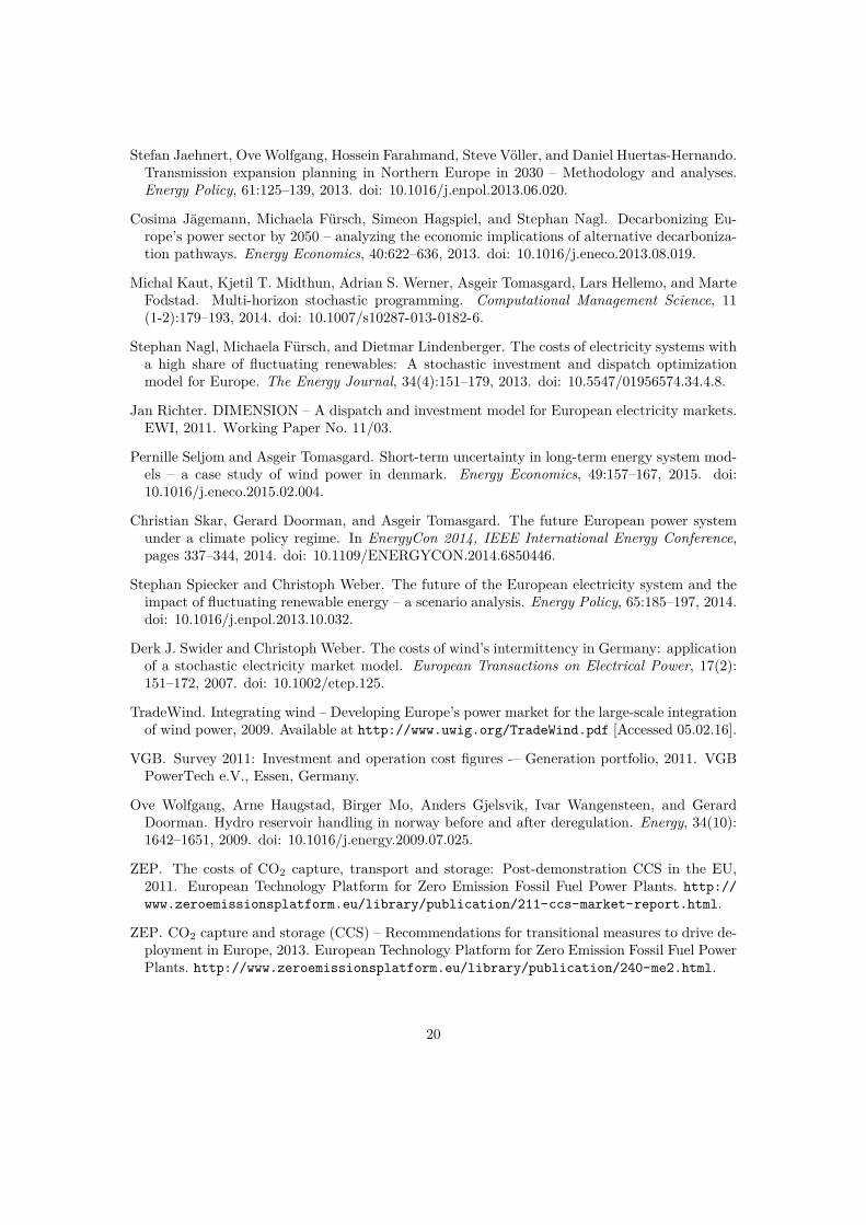
Figure 5: Fuel prices, electricity demand and carbon prices form EU 2013 Reference case. EC (2014)contains prices for hard coal, natural gas and oil. Lignite, uranium and biomass prices come from othersources, (ZEP, 2011; VGB, 2011), and are extrapolated from 2010 data.
(a) Select the hour h with the highest load value, i.e. the index h ∈ H full correspondingto the maximum element of τ loadhk′ h∈Hfull .
(b) The first extreme season of ξtype∗h0ω comprise the data from hours in the interval[h− 2, h+ 2] at the selected year k′ of τ type∗hk .
4. Form the other extreme peak seasons by obtaining the maximum load per node
τpeakloadnk′ = maxh∈Hfull
τ loadnhk′,
then selecting the |Speak| − 1 nodes n1, . . . , n|Speak|−1, with the highest load (where |Speak|is the number of extreme load seasons). Extreme load season j + 1 is formed by the hours[hj − 2, hj + 2], where hj is the hour with the highest hour load for node j.
After the procedure had been applied the sampled data profiles ξtype∗h0ω were checked to see thatthey closely match the mean and variance of the respective underlying raw data series. The loadand hydro base data profiles were further processed as described in the Appendix B.2.
3 EU reference scenario case study using EMPIREThe use of EMPIRE in a decarbonization study for the European power system is illustrated ona data set based on the EU reference case 2013 recently published by the European Commission(EC, 2014). This data set establishes the conditions for the long-term dynamics of the system,such as fuel prices and electricity demand development. A climate policy, in the form of a carbonprice, is also collected from the EU reference case. Some of the major assumptions are shown inFigure 5.
In this analysis we use four regular seasons, each with 48 consecutive hours, and six extremeload seasons, each with five consecutive hours. Three stochastic scenarios are used. All in all, thismeans that for each investment period a total of 666 dispatch hours are considered. Across all theinvestment periods a total of 5994 dispatch hours are used, establishing a diverse representationof different operating conditions. Appendix C provides further details regarding the input dataused for this analysis.
13

2010
2020
2030
2040
2050
0
500
1000
1500
Capacity [GW]
2010
2020
2030
2040
2050
0
2000
4000
Generation [TWh]
Solar PVWind OffshoreWind OnshoreHydro/Geo/OceanGas CCSBiomass Co-fir. CCSCoal CCSLignite CCSUnabated FossilNuclear
Figure 6: Optimal generation capacity and generation mix in the constrained transmission expansioncase. The category Hydro/Geo/Ocean comprises aggregated results for the technologies: hydroelec-tric power (reservoir and run-of-the-river), geothermal energy and ocean energy. Biomass Co-fir. is atechnology where 10 % biomass is cofired with hard coal.
2010
2020
2030
2040
2050
0
500
1000
1500
Capacity [GW]
2010
2020
2030
2040
2050
0
2000
4000
Generation [TWh]
Solar PVWind OffshoreWind OnshoreHydro/Geo/OceanGas CCSBiomass Co-fir. CCSCoal CCSLignite CCSUnabated FossilNuclear
Figure 7: Optimal generation capacity and generation mix in the constrained transmission expansioncase
Two transmission investment cases were developed for the purpose of this study. In thefirst case maximum capacities for HV line interconnectors were limited to two times their initialcapacity, plus an additional 1000 MW per interconnector. By basing the maximum limit oninstalled capacity, a degree of inertia is introduced in the infrastructure planning, while the1000 MW addition allows for moderate development of transmission corridors which are not ofsignificant capacity today. For each HV cable interconnector the total expansion was limited to1400 MW. For every time period the expansion for each HV line interconnector was limited to10 % of the initial capacity plus 300 MW. For HV cable interconnectors the limit was set to700 MW per time period. In the second case we did not allow for interconnector expansion.
The following sections presents the results from the two cases, and a discussion.
3.1 Aggregated results for EuropeThe European generation capacity and energy mixes for the EU reference case 2013 are displayedin Figure 6 (with interconnector expansion) and Figure 7 (no transmission expansion). At anEuropean level the differences are not tremendous, but some distinctions are worth pointingout. For onshore wind the installed capacity in 2050 is close to 530 GW in the case with
14

2010
2015
2020
2025
2030
2035
2040
2045
2050
0
500
1000
1334
201242
Emission [MtCO2/an]
Interconnector expansion No grid expansion20
1020
1520
2020
2520
3020
3520
4020
4520
50
40
50
60
70
37
6265
Average cost [e2010/MWh]
2010
2015
2020
2025
2030
2035
2040
2045
2050
0
200
400
131 142163
536
435
CCS and wind deployment [GW]
Wind (intercon. expansion)Wind (no grid expansion)CCS (intercon. expansion)CCS (no grid expansion)
Figure 8: Emissions, average electricity cost and deployment of CCS and wind (onshore/offshore)capacities for the cases with and without interconnector expansion.
interconnector capacity expansion, about 100 GW higher than in the no expansion case. Forsolar PV the installed capacity in 2050 is 127 GW in the interconnector expansion case, comparedto 117 GW in the no expansion. The additional renewable capacity seen in the interconnectorexpansion case reduces the need for thermal generation investments. For the no expansion case,unabated and CCS equipped fossil fuel generation capacities are, respectively, 43 GW and 21 GWhigher than for the grid expansion case. In the energy mix for the no expansion case, this resultsin 88 TWh additional generation from unabated fossil generation technologies and 134 TWhmore generation from CCS plants. This is offset by 171 TWh onshore wind and some additionalgeneration from other renewables in the interconnector expansion case.
Figure 8 shows the total emissions, average cost of electricity and deployment of CCS andwind generation capacities in Europe. The two cases start to diverge from 2020. Even beforethe most significant differences in wind investment emerge, there is a gap between the emissiontrajectories for the two cases. This can be attributed to better utilization of the low-carbongeneration capacities as more generation resources can be shared throughout the system. Theimpact of the increased levels of wind investments is seen to be larger for the average cost.An investigation of the different components of the system costs reveal that the difference iscaused by a lower fuel cost in the interconnector expansion case. This is to be expected aswind generation has zero fuel costs. For the CCS capacity the differences between the cases arenot considerable, however, the first CCS deployment is delayed by five years, until 2030, in theinterconnector expansion case.
3.2 Interconnector expansionThe initial transmission system design and the installed interconnector capacities in the expan-sion case are shown in Figure 9. In the initial system the total capacity was 67 GW, while theadditional interconnector expansion by 2050 ended up at 96 GW, yielding a total of 163 GW ca-pacity for all the interconnectors (we assume no decommissioning of the existing capacities). Theconstraints imposed on the expansion turn out to be binding for a majority of the connections.A total of 38 out of 55 interconnectors reach the maximum install limit. In particular, all the HV
15

Initial system 2010 Interconnector capacities 2050
No link0.5 GW1 GW2 GW3 GW4 GW5 GW10 GW
Figure 9: The initial (2010) interconnector capacities and the installed capacities in 2050.
cables links from Norway and Sweden are expanded to the maximum level. The same appliesfor the HV cables going from the UK to France, Belgium and the Netherlands. The connectionsalong the south-to-north axis going from Spain through France to Germany were also develop tothe maximum extent.
Most of the interconnectors with non-binding maximum expansion constraints are found inEastern Europe and the Balkans. In addition, the links between Germany and Austria, Germanyand Switzerland, and Germany and the Netherlands see non-binding constraints.
3.3 Generation capacities and energy mix by countryFigures 10 and 11 show the 2050 generation and energy mixes, in the two cases, for the tencountries with the highest electricity demand in Europe. The two cases are generally quitesimilar. In Germany there is a diverse mix of onshore wind (roughly 50 % of the generationcapacity and 20 % of the generation mix) and fossil fueled generation, both with and withoutCCS. In the generation mix CCS accounts for more than half the total energy produced. InFrance, nuclear power and onshore wind make up more than 70 % of both the capacity andenergy mix. Also, Italy, Great Britain and Spain see significant onshore wind deployment by2050. In Germany, Italy and Great Britain the maximum install constraints on onshore windcapacity are binding in 2050. In Great Britain and Poland unabated coal and lignite generationare displaced by CCS generation. Significant amounts of natural gas fired CCGTs are used inGermany, Italy, Great Britain, Spain and Belgium.
When it comes to the differences between the two transmission expansion cases the mostnotable countries are France, Poland and Norway. An additional 40 GW of onshore wind isdeployed in France, and 20 GW additional capacity is installed in both Poland and Norway, inthe interconnector expansion case. For solar PV the additional capacity in the interconnectorexpansion case is installed in France (6 GW), Italy (6 GW) and Spain (4 GW), while 5 GWis reduced elsewhere in Europe yielding a net increase of a bit more than 10 GW. The reducesamount of thermal generation capacity in the no expansion case over the alternative is distributedfairly evenly across all countries.
16

0 100 200 300
Others
FranceGermany
Italy
Great Brit.Spain
PolandNorway
Sweden
NetherlandsBelgium
Capacity [GW]
0 200 400 600 800 1000
Generation [TWh]
Solar PVWind offshoreWind onshoreHydro RoRHydro regulatedGeoWaveNuclearBio cofiring CCSBio cofiringOilGas CCSCCGTOCGTCoal CCSCoalLignite CCSLignite
Figure 10: Transmission capacity expansion case: Country-wise Baseline scenario result generationcapacity and generation mix in 2050.
0 100 200 300
Others
FranceGermany
Italy
Great Brit.Spain
PolandNorway
Sweden
NetherlandsBelgium
Capacity [GW]
0 200 400 600 800 1000
Generation [TWh]
Solar PVWind offshoreWind onshoreHydro RoRHydro regulatedGeoWaveNuclearBio cofiring CCSBio cofiringOilGas CCSCCGTOCGTCoal CCSCoalLignite CCSLignite
Figure 11: No transmission capacity case: Country-wise Baseline scenario result generation capacityand generation mix in 2050.
17

3.4 DiscussionFirstly, even with the current interconnector capacities installed in Europe there is a significantpotential for large-scale deployment of onshore wind. The results show a 25 % share in thegeneration mix for onshore wind without grid investments, and close to 30 % in for the casewith. It should be noted that the optimal interconnector expansion found, represents substantialinfrastructure investments, an increase of almost 150 % on top of today’s system. For solarPV, on the other hand, the effect of increased exchange capacity was modest. This implies thatcapital cost reductions are more important for solar deployment than grid investments.
Relative to 2010 levels, emissions are reduced by 85 % in the interconnector expansion caseand an 82 % reduction in the no expansion case. Without the ability to increase interconnec-tor capacities more CCS is deployed which essentially leads to more or less the same emissionreduction. In terms of costs, however, the differences turned out to be larger. As more windgeneration is deployed, accompanied by transmission expansion, less costs are incurred on fueland carbon. The capital costs are higher, but operational cost savings are high enough to leadto a 5 % net reduction in average cost by 2050, over the no expansion case.
The constraints imposed on maximum investments in generation and transmission capacitiesturn out to significantly affect the resulting system design. In the case without transmissionexpansion five of the ten countries with highest demand for electricity experience that the maxi-mum constraints on onshore wind expansion are binding. For the grid infrastructure a majorityof the constraints placed on interconnector expansion turned out to be binding. This means thathigher investments for both wind and interconnectors would likely have resulted from relaxingthese constraints. It can be difficult to determine the appropriate limits to use on investments,however carefully considerations should be used as the results are clearly sensitive to these pa-rameters.
4 Conclusions and further workThis paper provides a full methodological description of EMPIRE, a stochastic investment modelfor the European power system. The model features multiple investment periods, hourly dis-patch modeling for selected time segments of a year and multiple stochastic scenarios represent-ing operational uncertainty. This allows for simultaneous consideration of long-term dynamics,short-term dynamics and short-term uncertainty affecting investment decision and system oper-ation. These are all features which are particularly important when analyzing cases with highpenetrations of intermittent renewables as such technologies introduce a great deal of variabilityand uncertainty in the electricity supply. Computational tractability is achieved by utilizing amulti-horizon tree formulation, in which here-and-now operational decisions are decoupled fromfuture investment and operational decisions.
The case study presented illustrates the use of EMPIRE for a European decarbonizationstudy. Driven by the EU ETS price from the European reference case 2013 an emission reductionof more than 80 % is achieved displacing unabated fossil fuel generation with onshore wind andCCS. By allowing interconnector expansion, more wind power was deployed, which significantlyreduces the system operational costs. However only small differences are observed for the totalemissions.
There are two natural extensions to the work presented here. Firstly, the current version ofEMPIRE does not fully make use of the possibilities of the multi-horizon tree formulation. Byincorporating strategic uncertainty, which could for instance affect technology costs, fuel pricedevelopments or carbon price development, the effect of long-term uncertainty on decarbonization
18

pathways can be addressed. The second extension of the work is to develop algorithms forefficient solution of multi-horizon models. In particular decomposition methods, such as BendersDecomposition, mixed with parallel computing is a possible approach. By reducing computationtimes, and distributing computation tasks, it would be possible to considerably increase thenumber of stochastic operational scenarios used and get a better representation of the variabilityassociated with intermittent renewables. For the levels of wind deployment seen in the illustrationcases presented in this paper such considerations are extremely important for determining theneed for operational flexibility in the system.
AcknowledgmentThe authors gratefully acknowledge the support the Research Council of Norway R&D projectagreements no. 190913/S60 and 209697.
ReferencesJohn R. Birge and François Louveaux. Introduction to Stochastic Programming. Springer, NewYork, NY, 2nd ed edition, 2011. doi: 10.1007/978-1-4614-0237-4.
Jeroen de Joode, Ozge Ozdemir, Karina Veum, Adriaan van der Welle, Gianluigi Miglavacca,Alessandro Zani, and Angelo L’Abbate. SUSPLAN D.3: Trans-national infrastructure devel-opments on the electricity and gas market. Technical report, ECN, 2011.
EC. Council conclusions on EU position for the Copenhagen climate conference (7–18 december2009), 2009. Press release from the 2968th ENVIRONMENT Council meeting Luxembourg,21 October 2009.
EC. Energy roadmap 2050, 2011. COM (2011) 885 Final.
EC. EU energy, transport and GHG emissions trends to 2050. Reference scenario 2013, 2014.
ENTSO-E. Statistical database, 2012. Available from https://www.entsoe.eu/data/data-portal/.
EURELETRIC. Power statistics, 2011.
FICO R©. Xpress optimzation suite v7.9, 2015.
Michaela Fürsch, Stephan Nagl, and Dietmar Lindenberger. Optimization of power plant invest-ments under uncertain renewable energy deployment paths: A multistage stochastic program-ming approach. Energy Systems, pages 1–37, 2013. doi: 10.1007/s12667-013-0094-0.
Markus Haller, Sylvie Ludig, and Nico Bauer. Decarbonization scenarios for the EU and MENApower system: Considering spatial distribution and short term dynamics of renewable gener-ation. Energy Policy, 47:282–290, 2012. doi: 10.1016/j.enpol.2012.04.069.
Susanne Heipcke. Xpress–Mosel: Multi-solver, multi-problem, multi-model, multi-node modelingand problem solving. In Josef Kallrath, editor, Algebraic Modeling Systems, volume 104 ofApplied Optimization, chapter 5, pages 77–110. Springer-Verlag, Berlin Heidelberg, 2012. doi:10.1007/978-3-642-23592-4.
19
Stefan Jaehnert, Ove Wolfgang, Hossein Farahmand, Steve Völler, and Daniel Huertas-Hernando.Transmission expansion planning in Northern Europe in 2030 – Methodology and analyses.Energy Policy, 61:125–139, 2013. doi: 10.1016/j.enpol.2013.06.020.
Cosima Jägemann, Michaela Fürsch, Simeon Hagspiel, and Stephan Nagl. Decarbonizing Eu-rope’s power sector by 2050 – analyzing the economic implications of alternative decarboniza-tion pathways. Energy Economics, 40:622–636, 2013. doi: 10.1016/j.eneco.2013.08.019.
Michal Kaut, Kjetil T. Midthun, Adrian S. Werner, Asgeir Tomasgard, Lars Hellemo, and MarteFodstad. Multi-horizon stochastic programming. Computational Management Science, 11(1-2):179–193, 2014. doi: 10.1007/s10287-013-0182-6.
Stephan Nagl, Michaela Fürsch, and Dietmar Lindenberger. The costs of electricity systems witha high share of fluctuating renewables: A stochastic investment and dispatch optimizationmodel for Europe. The Energy Journal, 34(4):151–179, 2013. doi: 10.5547/01956574.34.4.8.
Jan Richter. DIMENSION – A dispatch and investment model for European electricity markets.EWI, 2011. Working Paper No. 11/03.
Pernille Seljom and Asgeir Tomasgard. Short-term uncertainty in long-term energy system mod-els – a case study of wind power in denmark. Energy Economics, 49:157–167, 2015. doi:10.1016/j.eneco.2015.02.004.
Christian Skar, Gerard Doorman, and Asgeir Tomasgard. The future European power systemunder a climate policy regime. In EnergyCon 2014, IEEE International Energy Conference,pages 337–344, 2014. doi: 10.1109/ENERGYCON.2014.6850446.
Stephan Spiecker and Christoph Weber. The future of the European electricity system and theimpact of fluctuating renewable energy – a scenario analysis. Energy Policy, 65:185–197, 2014.doi: 10.1016/j.enpol.2013.10.032.
Derk J. Swider and Christoph Weber. The costs of wind’s intermittency in Germany: applicationof a stochastic electricity market model. European Transactions on Electrical Power, 17(2):151–172, 2007. doi: 10.1002/etep.125.
TradeWind. Integrating wind – Developing Europe’s power market for the large-scale integrationof wind power, 2009. Available at http://www.uwig.org/TradeWind.pdf [Accessed 05.02.16].
VGB. Survey 2011: Investment and operation cost figures -– Generation portfolio, 2011. VGBPowerTech e.V., Essen, Germany.
Ove Wolfgang, Arne Haugstad, Birger Mo, Anders Gjelsvik, Ivar Wangensteen, and GerardDoorman. Hydro reservoir handling in norway before and after deregulation. Energy, 34(10):1642–1651, 2009. doi: 10.1016/j.energy.2009.07.025.
ZEP. The costs of CO2 capture, transport and storage: Post-demonstration CCS in the EU,2011. European Technology Platform for Zero Emission Fossil Fuel Power Plants. http://www.zeroemissionsplatform.eu/library/publication/211-ccs-market-report.html.
ZEP. CO2 capture and storage (CCS) – Recommendations for transitional measures to drive de-ployment in Europe, 2013. European Technology Platform for Zero Emission Fossil Fuel PowerPlants. http://www.zeroemissionsplatform.eu/library/publication/240-me2.html.
20

ZEP. CCS and the electricity market: Modelling the lowest-cost route to decarbon-ising European power, 2014. European Technology Platform for Zero Emission Fos-sil Fuel Power Plants. http://www.zeroemissionsplatform.eu/library/publication/253-zepccsinelectricity.html.
ZEP. CCS for industry – modelling the lowest-cost route to decarbonising Europe, 2015.European Technology Platform for Zero Emission Fossil Fuel Power Plants. http://www.zeroemissionsplatform.eu/library/publication/258-ccsforindustry.html.
A Nomenclature
Table 1: Paramters and variables in the EMPIRE model
Sets and indicesSet Index DescriptionN n Nodes (country)G g GeneratorsL l Interconnector links (unidirectional)A a Arcs (for directional flow)B b StoragesH h Operational hour (H− = H \ 1), |H| = H
S s SeasonI i Investment time period, |I| = I
Ω ω Stochastic scenario, |Ω| = O
T t Aggregated generator technologiesK k Years for historical data profilesDecision variablesSymbol Descriptionxgengi Generation capacity investmentxtranli Line capacity investmentxstorPWbi Storage power capacity investmentxstorENbi Storage energy capacity investmentygenghiω Generationyflowahiω Line flowychrgbhiω Storage chargeydischrgbhiω Storage dischargeyLLnhiω Energy not supplied (load shed)wstor
bhiω Storage energy content. Charge level = wstorbhiω/v
storENbi
vgengi Installed generation capacityvtranli Installed transmission capacityvstorPWbi Installed storage power capacityvstorENbi Installed storage energy capacityParametersSymbol Description
Continued on next page
21

Table 1 – Continued from previous pager Discount rateϑ Five year scale factor, ϑ =
∑4j=0(1 + r)−j = (1+r)5−1
r(1+r)4
πω Scenario probability,∑
ω∈Ω πω = 1, 0 ≤ πω ≤ 1.αs Seasonal scale factorcgengi Generator investment costctranli Transmission investment costcstorPWbi Storage power capacity investment costcstorENbi Storage energy capacity investment costqgengi Generator short-run marginal costqvollni Value of lost load at nodeξloadnhiω Loadξgenghiω Generator capacity availabilityξRegHydroLimgsiω Max energy production from regulated hydroξHydroLimniω Max energy production from hydro at nodeτ type∗hk Historical data series (type and ∗ indicate data profile type)xgengi Initial generation capacityxtranli Initial transmission capacityxstorPWbi Initial storage power capacityxstorENbi Initial storage energy capacityX
genti , V gen
ti Generation max build/install capacity (aggregate technology)X
tranli , V tran
li Transmission max build/install capacityX
storPWbi , V storPW
bi Storage power capacity max build/install capacityX
storENbi , V storEN
bi Storage energy capacity max build/install capacityilife∗ Life time for investment (∗ used as a wild-card for g, l, b)ηtranl Linear line efficiency. Loss = 1− ηtranl
ηchrgb Storage charge efficiencyηdischrgb Storage discharge efficiencyηroundtripb Storage round-trip efficiency, ηroundtripb = ηchrgb ηdischrgb
γgeng Generator ramp-up capabilityρb Storage discharge to charge power capacity ratioβb Storage power to energy capacity ratio
B Pre-processing of EMPIRE parametersB.1 Calculation of short-run marginal cost parametersThe variable operational costs of a particular type of technology can typically be split intoseparate components associated different parts of the power plant operation. A generic example,assuming internalization of emission costs, is
Variable costs = Fuel costs + Variable operation and maintenance costs+ Carbon emission cost + Carbon transport and storage costs
EMPIRE use linear cost functions, based on average heat rates, for all generators as seen in theobjective function. The coefficient of the generator production output variables can therefore be
22

Table 2: List and description of parameters used to calculate the generation cost coefficients.
Symbol Dimension Description
hr ti GJth/MWhe Heat rate (note: h = 3.6/efficiency)pFfi e/GJth Price of fuelpCi e/tCO2 Carbon emission price (tax or EUA)rf ccsti CCS removal fractionef tCO2/GJth Carbon content of fuelcvO&M
ti e/MWhe Variable operation and maintenance costcccsT&S
ti e/tCO2 Carbon storage and transport costqgengi e/MWh Marginal cost of generation (SRMC)
interpreted as the short-run marginal cost of production. In year i ∈ I, for a generator g ∈ G oftechnology t ∈ T using fuel f ∈ F be parameterized as
qgengi = hti · pFfi + cvO&Mti + hti · (1− rf ccsti ) · ef · pCi + hti · rf ccsti · ef · cccsT&S
ti . (7)
An overview of the symbols used can be found in Table 2.For conventional thermal generation burning fossil fuel no carbon is captured and stored
which means rf ccsti = 0. The variable cost expression therefore reduces to
qgengi = hr ti · pFfi + cvO&Mti + hr ti · ef · pCi . (8)
For nuclear power the assumed fuel carbon contents is assumed zero, i.e. ef = 0, yielding variablecost
qgengi = hr ti · pFfi + cvO&Mti . (9)
For renewable technologies pFfi = 0 and ef = 0, which leaves the variable cost simply equalingthe operation and maintenance cost
qgengi = cvO&Mti . (10)
B.2 Pre-processing baseline data seriesTable 3 gives an overview of the symbols used in this section. The baseline data series for hydropower production and load, obtained using the scenario generation routine discussed in themain article, were further transformed before being used as input to EMPIRE. The normalizedproduction profiles for wind power and solar PV production were used directly. The followingshows how the baseline series where used in EMPIRE
• Onshore and offshore wind power production and solar PV production:
ξgenghiω = ξgengh0ω, h ∈ H, g ∈ Gintermittent RES, i ∈ I, ω ∈ Ω.
Note: The underlying data series used to generate ξgengh0ω for renewable generators arenormalized production profiles. Therefore the baseline data series are also normalizedproduction values and can be used directly as input to EMPIRE.
23

Table 3: List and description of parameters processed after using the scenario generation routine.
Symbol DescriptionN Set of nodes (country)G Set of generators (superscript used to identify technology type)H Set of operational hoursS Set of seasonsI Set of investment time periodsΩ Set of stochastic scenariosπω Stochastic scenario probabilityαs Seasonal scale factore0n Annual demand in base year (historical)ein Annual demand for given investment period (target)ξtype∗h0ω Baseline data series (output from scenario generation)ξloadnhiω Loadξgenghiω Generator capacity availabilityξRegHydroLimgsiω Max energy production from regulated hydro
• Regulated hydro power production:
ξRegHydroLimgsiω =∑
h∈Hs
ξgenhg0ω, g ∈ GRegHydro, s ∈ S, i ∈ I, ω ∈ Ω.
Note: The underlying data series used to generate ξgen∗h0ω for regulated hydroelectric gener-ators are (synthetic) hourly production data. Summing these values over a time intervalwill therefore yield the total energy produces during this time.
• Load data series: In order to reflect development in demand for electricity from one invest-ment period to another the baseline load series are EMPIRE subject to a linear transfor-mation of the baseline data. For investment period i ∈ I assume that the target annualdemand for electricity in node n ∈ N is ein. The annual demand based on the baselineprofile data is denoted e0n. The actual demand data used in EMPIRE is then computedas
ξloadnhiω = ξloadnh0ω + ein − e0n
8760 , h ∈ H, n ∈ N , i ∈ I, ω ∈ Ω.
The new series have the desired annual demand since (for n ∈ N and i ∈ I)∑ω∈Ω
πω
∑s∈S
αs
∑h∈Hs
ξloadnhiω =∑ω∈Ω
πω
∑s∈S
αs
∑h∈Hs
ξloadnh0ω︸ ︷︷ ︸=e0n
+∑ω∈Ω
πω︸ ︷︷ ︸=1
∑s∈S
αs
∑h∈Hs︸ ︷︷ ︸
=8760
ein − e0n
8760 ,
= ein.
C Input data documentationC.1 Data sourcesThe input data used by EMPIRE has been collected from multiple sources. Hourly load timeseries for all countries in the model come from the ENTSO-E data portal (ENTSO-E, 2012).
24

Also net transfer capacities for cross-border exchange are based on ENTSO-E data. Normalizedproduction profiles for wind and solar generation for every country have been provided by thesame data material as was used by the EU funded project SUSPLAN (de Joode et al., 2011).Investment costs and generation technology specifications are provided exclusively from mem-bers of ZEP’s market economics group II and is documented in ZEP (2013). Initial generatortechnology installed capacity data are collected, and consolidated, from a number of differentsources including ENTSO-E, EURELECTRIC, EUR’Observer, NREAP and the following ISOand market operator’s websites: National Grid, Red Elèctrica, Terna, EEX.
C.2 Renewable energy potentialFor renewable generation technologies the maximum installed capacities are constrained by land-area available for deployment. For solar PV we assume that capacity per area unit is 150 W/m2,and we limit the total deployment of PV panels to cover at most 14 % of a country’s totalland-area. For onshore wind the capacity to area ratio is assumed to be 7 MW/km2, and themaximum installed capacity is based on limiting the total area use to 5 % of each country’sagricultural land-area. Wind offshore maximum capacity limits are based on the high windscenario published in the final report from the EU funded project TradeWind (2009). For coaland lignite we constrain the installed capacity to the maximum number found for each countryin the report EURELETRIC (2011) (plus a 10 % margin). The same applies for nuclear power.
D Input data for used for EMPIRE
Table 4: Investment cost for generation technologies, in e2010/kW. Source (ZEP, 2013).
2010 2015 2020 2025 2030 2035 2040 2045 2050Lignite 1600 1600 1600 1600 1600 1600 1600 1600 1600Lignite CCS 2600 2530 2470 2400 2330 2250Coal 1500 1500 1500 1500 1500 1500 1500 1500 1500Coal CCS 2500 2430 2370 2300 2230 2150Gas OCGT 400 400 400 400 400 400 400 400 400Gas CCGT 650 650 650 650 680 710 740 770 800Gas CCS 1350 1330 1310 1290 1270 1250Bio 10pcnt cofir. 1600 1600 1600 1600 1600 1600 1600 1600 1600Bio 10pcnt cofir. CCS 2600 2530 2470 2400 2330 2250Nuclear 3000 2838 2675 2513 2350 2188 2025 1863 1700Wave 6050 5669 5288 4906 4525 4144 3763 3381 3000Geo 5500 5500 5500 5500 5500 5500 5500 5500 5500Hydro regualted 3000 3000 3000 3000 3000 3000 3000 3000 3000Hydro run-of-river 4000 4000 4000 4000 4000 4000 4000 4000 4000Wind onshore 1200 1188 1175 1163 1150 1138 1125 1113 1100Wind offshore 4080 3930 3780 3630 3480 3330 3180 3030 2880Solar PV 1900 1788 1675 1563 1450 1338 1225 1113 1000
25

Table 5: Fixed operation and maintenance costs, in e2010/kW/an. Source (ZEP, 2013).
2010 2015 2020 2025 2030 2035 2040 2045 2050Liginite exist 32 32 32 32 32 32 32 32 32Lignite 32 32 32 32 32 32 32 32 32Lignite CCS 51 50 49 47 46 45Coal exist 31 31 31 31 31 31 31 31 31Coal 31 31 31 31 31 31 31 31 31Coal CCS 47 46 45 44 43 41Gas exist 20 20 20 20 20 20 20 20 20Gas OCGT 20 20 20 20 20 20 20 20 20Gas CCGT 30 30 30 30 35 40 45 49 54Gas CCS 47 50 54 58 61 65Oil exist 20 20 20 20 20 20 20 20 20Bio exist 48 47 46 45 44 43 42 41 40Bio 10pcnt cofir. 32 32 32 32 32 32 32 32 32Bio 10pcnt cofir. CCS 51 50 49 47 46 45Nuclear 134 131 127 123 120 116 112 108 105Wave 154 154 154 154 154 154 154 154 154Geo 92 92 92 92 92 92 92 92 92Hydro regualted 125 125 125 125 125 125 125 125 125Hydro run-of-river 125 125 125 125 125 125 125 125 125Wind onshore 54 54 53 52 51 50 49 48 47Wind offshore 138 133 128 122 117 112 107 102 96Solar PV 20 20 21 22 23 24 24 25 26
Table 6: Generator efficiency for thermal technologies, in percent. Source (ZEP, 2013).
2010 2015 2020 2025 2030 2035 2040 2045 2050Liginite exist 35 35 36 36 36 36 36 37 37Lignite 43 44 45 45 46 47 47 48 49Lignite CCS 37 39 40 41 42 43Coal exist 37 38 38 38 38 38 39 39 39Coal 45 46 46 47 47 47 48 48 49Coal CCS 39 40 41 41 42 43Gas exist 48 49 50 51 52 52 53 54 55Gas OCGT 40 40 41 41 41 41 41 42 42Gas CCGT 60 60 60 60 61 63 64 65 66Gas CCS 52 54 56 57 58 60Oil exist 38 38 38 38 38 38 38 38 38Bio exist 38 38 39 39 39 39 39 40 40Bio 10pcnt cofir. 45 46 46 47 47 47 48 48 49Bio 10pcnt cofir. CCS 39 40 41 41 42 43Nuclear 36 36 36 36 36 37 37 37 37
26

Table 7: Variable operation and maintenance (O& M) costs, in e2010/MWh. Source (ZEP, 2013). Thevariable O& M costs for oil, bio, hydro, wind and solar are added to the fixed O& M costs and reportedin Table 5.
2010 2015 2020 2025 2030 2035 2040 2045 2050Liginite exist 0.48 0.48 0.48 0.48 0.48 0.48 0.48 0.48 0.48Lignite 0.48 0.48 0.48 0.48 0.48 0.48 0.48 0.48 0.48Lignite CCS 3.28 3.28 3.28 3.28 3.28 3.28Coal exist 0.46 0.46 0.46 0.46 0.46 0.46 0.46 0.46 0.46Coal 0.46 0.46 0.46 0.46 0.46 0.46 0.46 0.46 0.46Coal CCS 2.46 2.46 2.46 2.46 2.46 2.46Gas exist 0.45 0.45 0.45 0.45 0.47 0.49 0.51 0.53 0.55Gas OCGT 0.45 0.45 0.45 0.45 0.47 0.49 0.51 0.53 0.55Gas CCGT 0.45 0.45 0.45 0.45 0.52 0.59 0.66 0.73 0.80Gas CCS 1.85 1.92 1.99 2.06 2.13 2.20Bio 10pcnt cofir. 0.48 0.48 0.48 0.48 0.48 0.48 0.48 0.48 0.48Bio 10pcnt cofir. CCS 3.28 3.28 3.28 3.28 3.28 3.28Nuclear 1.80 1.75 1.70 1.65 1.60 1.55 1.50 1.45 1.40
Table 8: Transport and storage costs assumed for carbon capture and storage technologies, ine2010/tCO2.
2025 2030 2035 2040 2045 2050CCS T&S cost 19 18 17 15 14 13
Table 9: Derived short-run marginal costs for the various technologies, in e2010/MWh. Omittedtechnologies have SRMC less than 1 e/MWh.
2010 2015 2020 2025 2030 2035 2040 2045 2050Liginite exist 9 9 26 32 38 44 56 68 81Lignite 7 7 21 25 30 34 43 52 61Lignite CCS 30 29 28 27 27 26Coal exist 15 15 31 37 42 48 59 70 81Coal 13 13 26 30 34 39 48 56 65Coal CCS 35 34 33 32 32 31Gas exist 30 29 36 39 41 44 49 55 60Gas OCGT 36 36 44 48 52 55 63 71 79Gas CCGT 24 24 30 33 35 37 42 46 50Gas CCS 38 37 37 37 38 39Oil exist 69 70 85 92 99 106 118 128 138Bio exist 47 47 47 44 42 45 47 49 53Bio 10pcnt cofir. 15 15 27 31 34 39 47 55 63Bio 10pcnt cofir. CCS 37 35 34 32 31 30Nuclear 7 8 8 8 8 8 9 9 10
27

Table 10: Interconnector expansion costs. Given in e2010/MW/km. Based on (de Joode et al., 2011).
2010 2015 2020 2025 2030 2035 2040 2045 2050HV lines 719 719 662 662 604 604 604 604 604HV cables 2769 2769 2769 2769 2160 2160 1551 1551 1551
28

Table 11: Initial capacities for the ten countries with the highest installed capacity in 2010, and the other countries aggregated, as assumedin EMPIRE. Numbers in GW. Italy also has 1 GW installed capacity of geothermal generation, but this has been omitted from the table forbrevity. Data from a number of different sources including ENTSO-E, EURELECTRIC, EUR’Observer, NREAP and the following ISO andmarket operator’s websites: National Grid, Red Elèctrica, Terna, EEX
Liginite Coal Gas Oil Bio Nuclear Hydro Wind Solar PVregulated run-of-river onshore offshore
Others 26 19 41 11 7 23 26 18 19 2 12Germany 21 27 23 10 8 12 1 3 38 2 38France 8 11 9 1 63 14 8 9 6Italy 20 47 8 2 9 5 9 18Great Brit. 28 32 4 4 10 1 1 8 4 5Spain 12 27 4 1 8 13 3 23 5Sweden 1 4 3 10 10 7 5Poland 10 20 1 4Norway 1 22 6 1Netherlands 4 18 1 3 1Romania 4 1 4 1 4 2 3 1Europe 61 140 204 50 27 126 100 52 122 9 87
29

Table 12: Maximum installed capacity limits for the ten countries with the highest installed capacity in 2010, and the other countries aggregated,as assumed in EMPIRE. Numbers in GW. For Lignite and Coal the limit applies to the sum unabated and CCS capacity. Generation technologiesusing natural gas are not limited.
Lignite Coal Nuclear Hydro Wind Solar PVregulated run-of-river onshore offshore
Others 30 28 32 54 60 282 39 329Germany 23 34 2 4 70 106 75France 14 65 21 16 105 27 114Italy 7 13 9 60 3 63Great Brit. 48 17 7 3 53 68 51Spain 12 12 40 10 88 22 106Sweden 1 8 11 7 105 24 94Poland 10 27 3 1 2 70 66Norway 30 15 70 13 68Netherlands 9 4 9 42 9Romania 5 2 5 11 7 42 5 50Europe 66 183 145 190 132 952 350 1024
30