A MONTE CARLO SIMULATION ANALYSIS OF THE BEHAVIOR

OF A FINANCIAL INSTITUTION’S RISK

by Hannah Folz

A thesis submitted to Johns Hopkins University in conformity with the requirements for the degree of Master of Science in Engineering

Baltimore, Maryland

April, 2017

© 2017 Hannah Folz All Rights Reserved

ii

Abstract

For this exploration, Monte Carlo simulations are performed on a time series

model of a financial institution to make assessments about outcome probabilities. Three

different scenarios are being explored, Baseline, Adverse and Severely Adverse; to

compare the effect that increasingly severe macroeconomic conditions have on financial

risk. These will be visualized through the Monte Carlo simulations.

The Monte Carlo simulations are performed on an AR(1) model,

Yt =αYt−1 +β1x1t−1 +β2x2t−1 +et , which is fitted using linear regression. Past data of the

net loss of loans and leases of Bank of America is used in conjunction with

macroeconomic data to determine the best combination of macroeconomic variables in

addition to their parameters.

The Monte Carlo simulations serve as a powerful tool for quantifying the risk of

adverse outcomes and for making assessments about the behavior of the time series risk

model under the three different scenarios.

Advisor: Daniel Naiman

iii

Preface

With deepest gratitude and appreciation, I would like to thank the following people for

their support of this Masters Thesis.

Daniel Naiman – for encouraging me to challenge myself with my thesis, and for his

unrelenting guidance with this.

Donniell Fishkind – for his commitment to my personal and intellectual growth

throughout my time at Hopkins.

Jason Dulnev – for his inspiration to pursue this topic.

Family and friends – for their love, support and faith in me.

iv

Table of Contents

Abstract.......................................................................................................................................ii

Preface........................................................................................................................................iii

Table of Contents.....................................................................................................................iv

List of Tables.............................................................................................................................vi

List of Figures..........................................................................................................................vii

Introduction................................................................................................................................1

Goal........................................................................................................................................................1Background..........................................................................................................................................1Methodology........................................................................................................................................2Applications.........................................................................................................................................4

Linear Regression based on Macroeconomic Data............................................................6

Approach..............................................................................................................................................6Timeframe............................................................................................................................................6Determining Theoretical Values for Yt and Yt−1 .........................................................................7Determining the Macroeconomic Variables and Coefficient Values used in the Linear Regression.............................................................................................................................................9Evaluation of Dependent and Independent Variables Selection............................................14Assumptions and limitations..........................................................................................................16

Monte Carlo Simulations.......................................................................................................18

AR(1) Model.......................................................................................................................................18Residual...............................................................................................................................................19Data under the three Scenarios.....................................................................................................20Realizations – 15 Quarters of Simulated Data...........................................................................2410,000 Trials for the Monte Carlo Simulations..........................................................................25Additional Considerations..............................................................................................................25

What If Analysis......................................................................................................................27

Analyses..............................................................................................................................................27Threshold Analysis...........................................................................................................................27

v

Statistical Analysis............................................................................................................................32Conclusion................................................................................................................................41

Summary............................................................................................................................................41Future opportunities for research.................................................................................................41Applications.......................................................................................................................................42

Variables and Abbreviations................................................................................................43

Appendices................................................................................................................................44

Appendix 1: Macroeconomic Variable Analysis........................................................................44Appendix 2: Setting up the Baseline Scenario............................................................................46Appendix 3: Sample Analysis.........................................................................................................48

Bibliography.............................................................................................................................53

Curriculum Vitae....................................................................................................................55

vi

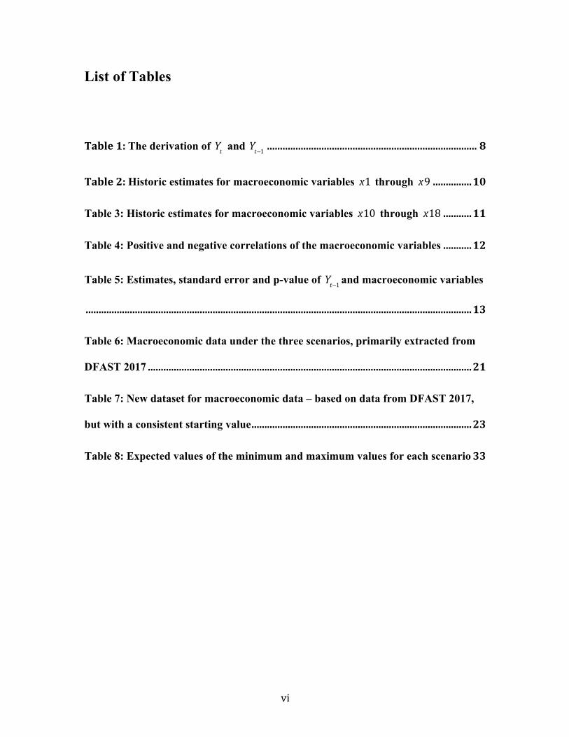
List of Tables

Table1:The derivation of Yt and Yt−1 .................................................................................8

Table2:Historic estimates for macroeconomic variables x1 through x9 ...............10

Table 3: Historic estimates for macroeconomic variables x10 through x18 ...........11

Table 4: Positive and negative correlations of the macroeconomic variables...........12

Table 5: Estimates, standard error and p-value of Yt−1 and macroeconomic variables

.....................................................................................................................................................13

Table 6: Macroeconomic data under the three scenarios, primarily extracted from

DFAST 2017.............................................................................................................................21

Table 7: New dataset for macroeconomic data – based on data from DFAST 2017,

but with a consistent starting value.....................................................................................23

Table 8: Expected values of the minimum and maximum values for each scenario33

vii

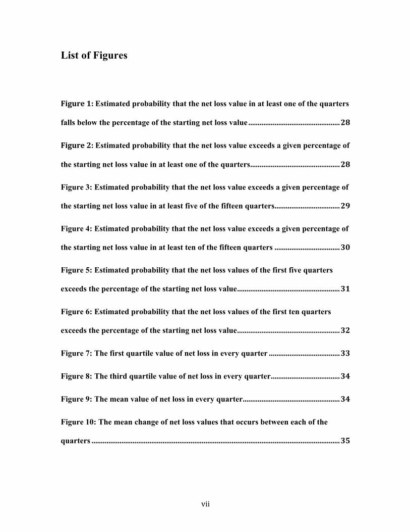
List of Figures

Figure1:Estimated probability that the net loss value in at least one of the quarters

falls below the percentage of the starting net loss value.................................................28

Figure2:Estimated probability that the net loss value exceeds a given percentage of

the starting net loss value in at least one of the quarters................................................28

Figure 3: Estimated probability that the net loss value exceeds a given percentage of

the starting net loss value in at least five of the fifteen quarters...................................29

Figure 4: Estimated probability that the net loss value exceeds a given percentage of

the starting net loss value in at least ten of the fifteen quarters...................................30

Figure 5: Estimated probability that the net loss values of the first five quarters

exceeds the percentage of the starting net loss value.......................................................31

Figure 6: Estimated probability that the net loss values of the first ten quarters

exceeds the percentage of the starting net loss value.......................................................32

Figure 7: The first quartile value of net loss in every quarter......................................33

Figure 8: The third quartile value of net loss in every quarter.....................................34

Figure 9: The mean value of net loss in every quarter....................................................34

Figure 10: The mean change of net loss values that occurs between each of the

quarters.....................................................................................................................................35

viii

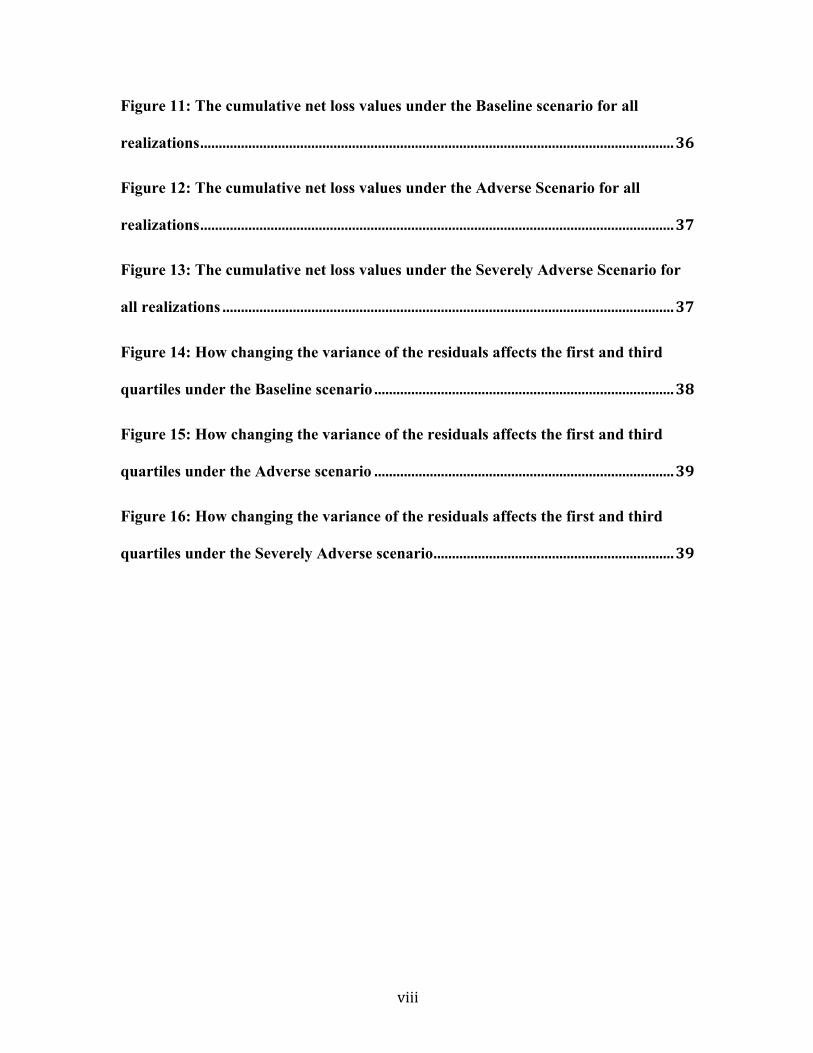
Figure 11: The cumulative net loss values under the Baseline scenario for all

realizations................................................................................................................................36

Figure 12: The cumulative net loss values under the Adverse Scenario for all

realizations................................................................................................................................37

Figure 13: The cumulative net loss values under the Severely Adverse Scenario for

all realizations..........................................................................................................................37

Figure 14: How changing the variance of the residuals affects the first and third

quartiles under the Baseline scenario.................................................................................38

Figure 15: How changing the variance of the residuals affects the first and third

quartiles under the Adverse scenario.................................................................................39

Figure 16: How changing the variance of the residuals affects the first and third

quartiles under the Severely Adverse scenario.................................................................39

1

Introduction

Goal

By performing Monte Carlo simulations on a time series risk model, synthetic

datasets can be analyzed in depth, enabling one to project future expected behavior and

quantify the chance of a extreme event.

Background

Pre Provision Net Revenue (PPNR) models are used to solve for the anticipated

net revenue prior to removing the expected losses incurred. They are the net revenue

generated before loss provisions are adjusted for, and for a bank, net revenue = net

interest income + non-interest income – expenses1. Due to the financial crisis, banks are

required to perform two types of stress tests – the Comprehensive Capital Analysis and

Review (CCAR) and Dodd-Frank Act Stress Test (DFAST). These stress tests measure

losses banks expect to incur under baseline macroeconomic conditions, in addition to

adverse and severely adverse macroeconomic conditions2. These will be referred to as

Baseline, Adverse and Severely Adverse scenarios respectively. The financial risk

models created through stress testing often involve two to three macroeconomic

1 Campbell, Harvey R. "Definition of "Pre-Provision Net Revenue"." NASDAQ. N.p., 2011. Web. 07 Apr. 2017. <http://www.nasdaq.com/investing/glossary/p/pre-provision-net-revenue>. 2 "FRB: Supervisory Scenarios, Dodd-Frank Act Stress Test 2016: Supervisory Stress Test Methodology and Results June-2016." FRB: Supervisory Scenarios, Dodd-Frank Act Stress Test 2016: Supervisory Stress Test Methodology and Results June-2016. N.p., 9 Aug. 2016. Web. 07 Apr. 2017. <https://www.federalreserve.gov/bankinforeg/stress-tests/2016-Supervisory-Scenarios.htm>.

2

variables. PPNR models are created based on time series data, and fitted using least-

squares regression. It is important to note that the time series regressions are not modeled

at the granular level of individual accounts, but rather, by examining the expected

revenue, losses or portfolio value of a large bank or several banks. For the purposes of

this exploration, the dependent variable is the net losses to the loans and leases of Bank

of America.

When creating these models, and using them to project the anticipated net losses,

several conditions are assumed to hold true. These include order correlation, stationarity,

homoscedasticity, collinearity, normality of residuals, independence of residuals,

amongst others. It is possible to test whether these conditions actually hold true, to

confirm that the assumptions of the model indeed hold. For the purposes of this paper, it

will be assumed that these conditions hold, and limitations of this assumption will be

discussed throughout, as the focus of the exploration is on using a fitted model to

quantify risk under various scenarios. This endeavor involves the investigation of

recurring patterns of datasets, so that conclusions about projected outcomes based on

three different scenarios – the Baseline, Adverse and Severely Adverse scenarios – can be

drawn.

Methodology

Monte Carlo simulations are performed to create realizations, which are datasets

of 15 quarters. Through this, 10,000 trials of randomly simulated data are generated

under three different scenarios.

3

The focus is on AR(1) processes, and thus the following notation will be used for

the model: Yt =αYt−1 +β1x1t−1 +β2x2t−1 +et . The macroeconomic variables, x1t−1 and

x2t−1 , are the independent variables, while net loss, Yt−1 , is the dependent variable. The

coefficients α , β1 and β2 are constants that are fitted using historical data. Finally et ,

is a random normal variable with mean=0 and variance=σ 2 .

In order to create as accurate a model as possible, the historical data of 18 quarters

from March 2003 (Q1 2003) to June 2007 (Q2 2007) of net loss will be used, so that the

best performing combination of macroeconomic variables, x1t−1 and x2t−1 can be

identified. Most of the macroeconomic conditions are derived from the DFAST 2017

report by the Federal Reserve Bank of St. Louis, and the net loss data is derived from the

Federal Deposit Insurance Corporation (FDIC). Using a linear regression, the respective

weights, β1 and β2 , and the weight α of Yt−1 will be fitted. The standard deviation of

et is also fitted, as it is the residual standard error. By performing a linear regression, the

combination of two macroeconomic variables and Yt−1 , which has the strongest fit to the

18 quarters of historic data, will be identified – in addition to the values of α , β1 and

β2 and et , which result in this strong fit.

Having found an AR(1) model with a good fit against the historic dataset of 18

quarters, 10,000 trials of randomly simulated data will be generated under three

scenarios. In the Baseline, Adverse and Severely Adverse scenarios, the previously found

values of α , β1 and β2 serve as constants – they are dynamic values, which are fixed.

4

The value of et will be randomly generated for every quarter in every realization under

each scenario – as a random normal variable, where the mean is 0, but the standard

deviation is the previously computed value for the residual standard error. For each of the

scenarios, differing values for the macroeconomic variables will be used, since they are

future projected values, ranging from September 2016 (Q3 2016) to March 2020 (Q1

2020). Thus the value of Yt−1 in the first quarter, September 2016, is fixed, and the future

values will be changing, and calculated based on the previous Yt results (in the t +1

quarter, Yt becomes Yt−1 ). The dynamics of the system describing the evolution of net

loss (where net loss is taken as driven by the macroeconomic variables which take

prescribed, forecasted values) are assumed to henceforth apply in the future. Further

analysis will be conducted on each realization.

Applications

This exploration of time series models is important because a lack of estimating

future projected net losses can impact financial institutions and therefore also their clients

in a negative way. Being able to project expected net losses under a variety of differing

macroeconomic scenarios creates feelings of security and safety, which are needed in

today’s economy. Mandated stress testing, with DFAST and CCAR regulations, was

implemented in response to the financial crisis – as creating financial risk models that

take stress testing into consideration are seen as beneficial to both the financial institution

and its clients. There are also significant outcomes for other stakeholders, such as

investors or anyone working in the real estate domain.

5

Although the time series model created in this exploration applies to a particular

bank and the specific Yt variable of net losses on loans and leases, the methodology can

be extracted and applied in other contexts as well. In particular, the occurrence analysis is

a powerful tool for identifying how likely rare events are, as it involves measuring in how

many realizations (which is one set of 15 quarters in the simulation) a certain threshold

value is surpassed. Estimating values for the cumulative net loss, mean net loss and the

first and third quartiles of the net loss under the three scenarios, is a powerful

comparative tool to see what effect a change in the macroeconomic environment has.

Other industries – such as the insurance, healthcare or tourism industry – could also

benefit from analyzing how changes in the macroeconomic environment affect their

clients’ behavior and therefore their net revenues.

6

Linear Regression based on Macroeconomic Data

Approach

To determine which combination of macroeconomic variables results in the best

fit for the financial risk model, the LM function (Linear Model) in R will be applied, to

find a linear regression of macroeconomic variables in combination with Yt−1 , which is

the value of the net loss on loans and leases of a bank.

Timeframe

The timeframe ranges from March 2003 (Q1 2003) to June 2007 (Q2 2007)

inclusively. The data is computed quarterly, and thus involves 18 data points. The

timeframe is restricted to this range of historic observations, as it is before the financial

crisis and thus abides by normal, expected macroeconomic conditions. Both the

dependent variable (the net loss incurred) and the independent variables (the

macroeconomic conditions) perform and interact in an expected, understandable way.

Data thereafter – of both the macroeconomic conditions, and therefore also of the

dependent variable, net loss – is affected by the financial crisis of 2008. Thus the time

period of 18 quarterly data points from Q1 2003 until Q2 2007 provides a reasonable

environment from which to draw conclusions about expected macroeconomic conditions,

which is the focus of this exploration.

7

Determining Theoretical Values for Yt and Yt−1

As mentioned previously, Yt−1 is defined as the value of the net loss on loans and

leases at time t −1 , which is used as part of the AR(1) model to find a value for Yt , the

net loss at time t . The values of Yt are derived from the “Net Loss to Average Total

Loans and Leases” for Bank of America from the Federal Financial Institutions

Examination Council (FFIEC) report3. The value for “Net Loss to Average Total

LN&LS” for Bank of America was extracted from FFIEC’s Summary Ratios’ page. For

example, for March 2003 (Q1 2003), the value is 0.6%. This is “Net Loss as a percent of

Average Total Loans and Leases”, and is defined as “Gross loan and lease charge-off,

less gross recoveries (includes allocated transfer risk reserve charge-off and recoveries),

divided by average total loans and leases”4. This percentage was converted to a decimal:

0.006. Next, the value of “Net Loans and Leases” was found via FDIC’s Balance Sheet

$ page. This is defined as “Gross loans and leases, less allowance and reserve and

unearned income”5. The value is $327,629,000 for Q1 2003, and to calculate Yt , the

decimal value of “Net Loss to Average Total LN&LS” was multiplied by “Net Loans and

3 "View -- Uniform Bank Performance Report." FFIEC Central Data Repository's Public Data Distribution. Federal Financial Institutions Examination Council, n.d. Web. 07 Apr. 2017. <https://cdr.ffiec.gov/public/Reports/UbprReport.aspx?rptCycleIds=87%2C82%2C86%2C81%2C76&rptid=283&idrssd=480228&peerGroupType=&supplemental=>. 4 "Uniform Bank Performance Report Interactive User's Guide." FFIEC Central Data Repository's Public Data Distribution. Federal Financial Institutions Examination Council, n.d. Web. 07 Apr. 2017. <https://cdr.ffiec.gov/Public/Reports/InteractiveUserGuide.aspx?LineID=609712&Rssd=480228&PageTitle=Summary%2BRatios&Concept=UBPRE019&ReportDate=3%2F31%2F2016>. 5 "Uniform Bank Performance Report Interactive User's Guide." FFIEC Central Data Repository's Public Data Distribution. Federal Financial Institutions Examination Council, n.d. Web. 07 Apr. 2017. <https://cdr.ffiec.gov/Public/Reports/InteractiveUserGuide.aspx?LineID=609957&Rssd=480228&PageTitle=Balance%2BSheet%2B%24&Concept=UBPRE119%2CUBPRE141%2CUBPRE027&ReportDate=3%2F31%2F2016>.

8

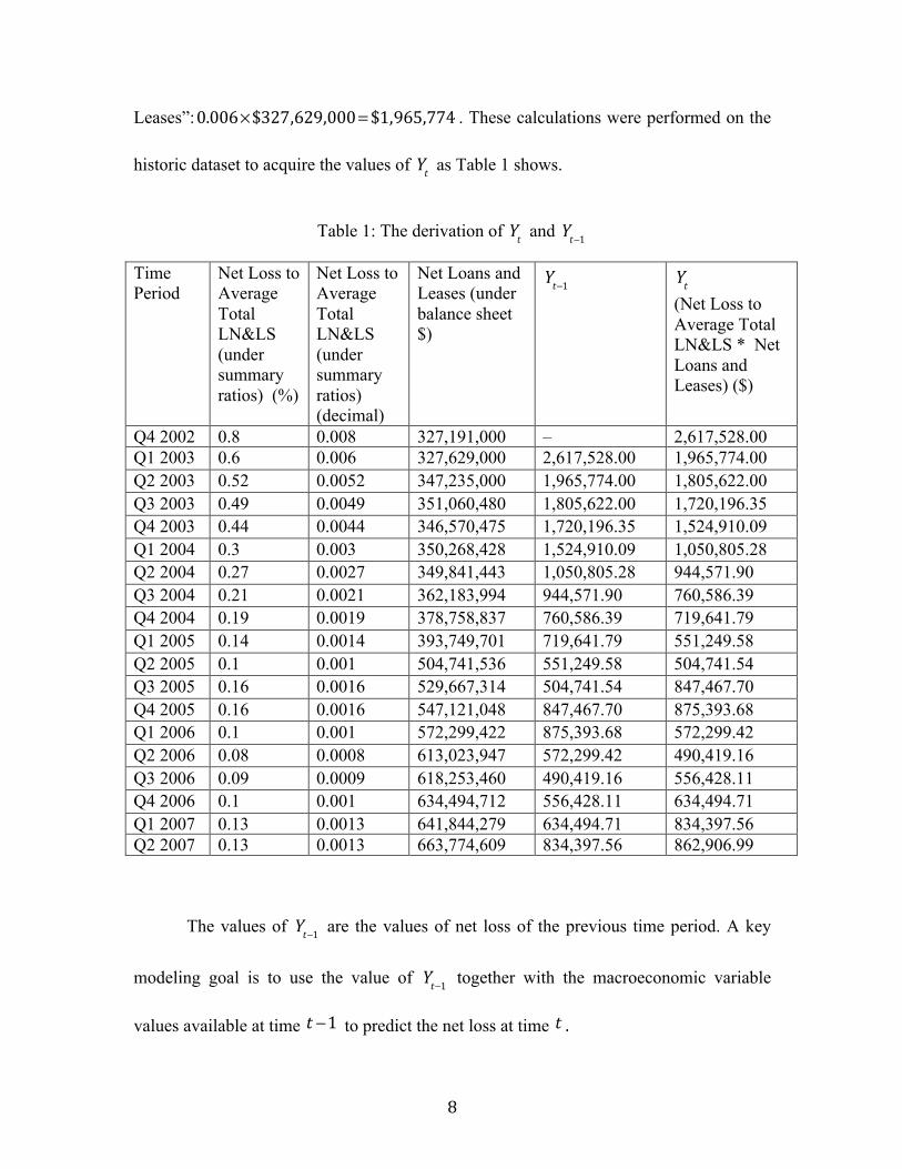
Leases”:0.006×$327,629,000= $1,965,774 . These calculations were performed on the

historic dataset to acquire the values of Yt as Table 1 shows.

Table 1: The derivation of Yt and Yt−1

Time Period

Net Loss to Average Total LN&LS (under summary ratios) (%)

Net Loss to Average Total LN&LS (under summary ratios) (decimal)

Net Loans and Leases (under balance sheet $)

Yt−1 Yt

(Net Loss to Average Total LN&LS * Net Loans and Leases) ($)

Q4 2002 0.8 0.008 327,191,000 – 2,617,528.00 Q1 2003 0.6 0.006 327,629,000 2,617,528.00 1,965,774.00 Q2 2003 0.52 0.0052 347,235,000 1,965,774.00 1,805,622.00 Q3 2003 0.49 0.0049 351,060,480 1,805,622.00 1,720,196.35 Q4 2003 0.44 0.0044 346,570,475 1,720,196.35 1,524,910.09 Q1 2004 0.3 0.003 350,268,428 1,524,910.09 1,050,805.28 Q2 2004 0.27 0.0027 349,841,443 1,050,805.28 944,571.90 Q3 2004 0.21 0.0021 362,183,994 944,571.90 760,586.39 Q4 2004 0.19 0.0019 378,758,837 760,586.39 719,641.79 Q1 2005 0.14 0.0014 393,749,701 719,641.79 551,249.58 Q2 2005 0.1 0.001 504,741,536 551,249.58 504,741.54 Q3 2005 0.16 0.0016 529,667,314 504,741.54 847,467.70 Q4 2005 0.16 0.0016 547,121,048 847,467.70 875,393.68 Q1 2006 0.1 0.001 572,299,422 875,393.68 572,299.42 Q2 2006 0.08 0.0008 613,023,947 572,299.42 490,419.16 Q3 2006 0.09 0.0009 618,253,460 490,419.16 556,428.11 Q4 2006 0.1 0.001 634,494,712 556,428.11 634,494.71 Q1 2007 0.13 0.0013 641,844,279 634,494.71 834,397.56 Q2 2007 0.13 0.0013 663,774,609 834,397.56 862,906.99

The values of Yt−1 are the values of net loss of the previous time period. A key

modeling goal is to use the value of Yt−1 together with the macroeconomic variable

values available at time t −1 to predict the net loss at time t .

9

Determining the Macroeconomic Variables and Coefficient Values used in the

Linear Regression

The combination of macroeconomic variables to be used is determined by

minimizing the Akaike Information Criterion (AIC), which is calculated using the

residual sum of squares in a regression. It captures the trade-off between the accuracy of

the fit and the complexity of the model creating this fit (with the goal of creating an

accurate fit with little complexity). In this situation, the issue of how many variables to

include in the model is avoided by forcing the number of macroeconomic variables

included to be two. Hence, the AIC reduces to simply looking at a residual sum of

squares.

The macroeconomic variables that are tested include Real GDP Growth ( ),

Nominal GDP Growth (x2), Real Disposable Income Growth (x3), Nominal Disposable

Income Growth (x4 ), Unemployment Rate (x5 ), CPI Inflation Rate (x6 ), 3-Month

Treasury Rate (x7 ), 5-Year Treasury Rate (x8 ), 10-Year Treasury Rate (x9 ), BBB

Corporate Yield (x10 ), Mortgage Rate (x11 ), Prime Rate (x12), Dow Jones Total

Stock Market Index (x13), House Price Index (x14 ), Commercial Real Estate Price

Index (x15 ), Market Volatility Index (x16 ), Gross National Product (x17 ), and

Effective Federal Funds Rate (x18 ).

The Dow Jones Total Stock Market Index was derived from the 2016 DFAST

report, since it was more precise (with five rather than four significant figures)6. Gross

National Product and Effective Federal Funds Rate values were derived from the Federal 6 "2016 Supervisory Scenarios for Annual Stress Tests Required under the Dodd-Frank Act Stress Testing Rules and the Capital Plan Rule." DFAST. Board of Governors of the Federal Reserve System, 2016. Web. 7 Apr. 2017. <http://www.federalreserve.gov/newsevents/press/bcreg/bcreg20160128a2.pdf>.

x1

10

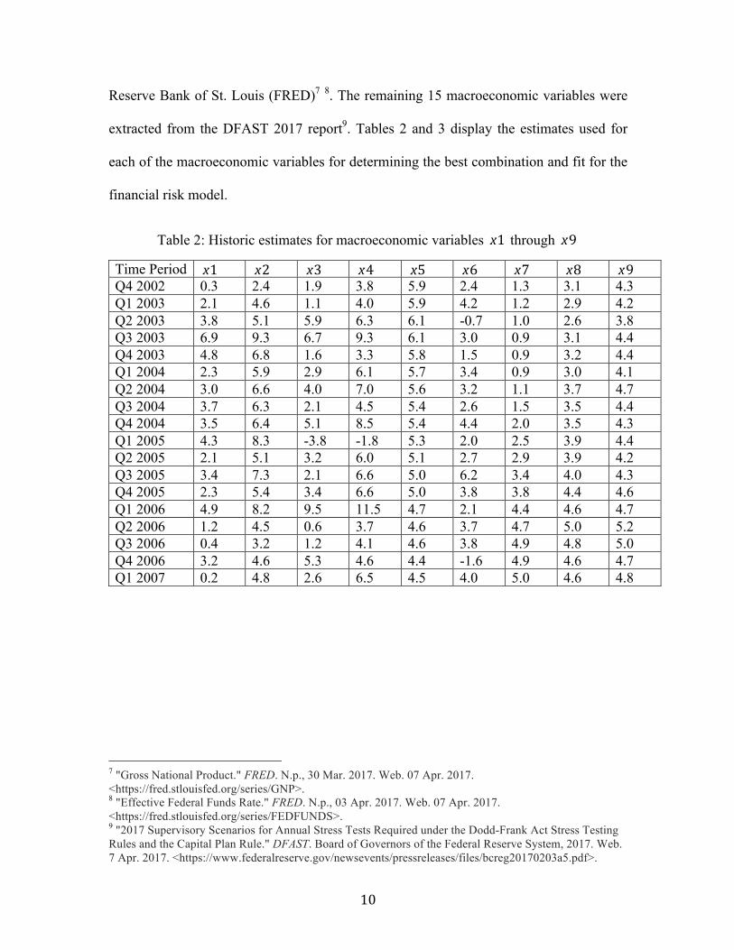
Reserve Bank of St. Louis (FRED)7 8. The remaining 15 macroeconomic variables were

extracted from the DFAST 2017 report9. Tables 2 and 3 display the estimates used for

each of the macroeconomic variables for determining the best combination and fit for the

financial risk model.

Table 2: Historic estimates for macroeconomic variables x1 through x9

Time Period x1 x2 x3 x4 x5 x6 x7 x8 x9 Q4 2002 0.3 2.4 1.9 3.8 5.9 2.4 1.3 3.1 4.3 Q1 2003 2.1 4.6 1.1 4.0 5.9 4.2 1.2 2.9 4.2 Q2 2003 3.8 5.1 5.9 6.3 6.1 -0.7 1.0 2.6 3.8 Q3 2003 6.9 9.3 6.7 9.3 6.1 3.0 0.9 3.1 4.4 Q4 2003 4.8 6.8 1.6 3.3 5.8 1.5 0.9 3.2 4.4 Q1 2004 2.3 5.9 2.9 6.1 5.7 3.4 0.9 3.0 4.1 Q2 2004 3.0 6.6 4.0 7.0 5.6 3.2 1.1 3.7 4.7 Q3 2004 3.7 6.3 2.1 4.5 5.4 2.6 1.5 3.5 4.4 Q4 2004 3.5 6.4 5.1 8.5 5.4 4.4 2.0 3.5 4.3 Q1 2005 4.3 8.3 -3.8 -1.8 5.3 2.0 2.5 3.9 4.4 Q2 2005 2.1 5.1 3.2 6.0 5.1 2.7 2.9 3.9 4.2 Q3 2005 3.4 7.3 2.1 6.6 5.0 6.2 3.4 4.0 4.3 Q4 2005 2.3 5.4 3.4 6.6 5.0 3.8 3.8 4.4 4.6 Q1 2006 4.9 8.2 9.5 11.5 4.7 2.1 4.4 4.6 4.7 Q2 2006 1.2 4.5 0.6 3.7 4.6 3.7 4.7 5.0 5.2 Q3 2006 0.4 3.2 1.2 4.1 4.6 3.8 4.9 4.8 5.0 Q4 2006 3.2 4.6 5.3 4.6 4.4 -1.6 4.9 4.6 4.7 Q1 2007 0.2 4.8 2.6 6.5 4.5 4.0 5.0 4.6 4.8

7 "Gross National Product." FRED. N.p., 30 Mar. 2017. Web. 07 Apr. 2017. <https://fred.stlouisfed.org/series/GNP>. 8 "Effective Federal Funds Rate." FRED. N.p., 03 Apr. 2017. Web. 07 Apr. 2017. <https://fred.stlouisfed.org/series/FEDFUNDS>. 9 "2017 Supervisory Scenarios for Annual Stress Tests Required under the Dodd-Frank Act Stress Testing Rules and the Capital Plan Rule." DFAST. Board of Governors of the Federal Reserve System, 2017. Web. 7 Apr. 2017. <https://www.federalreserve.gov/newsevents/pressreleases/files/bcreg20170203a5.pdf>.

11

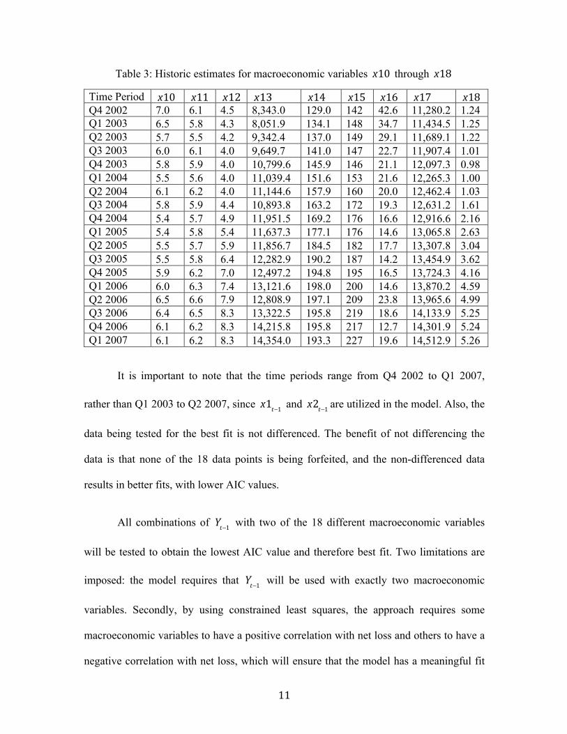
Table 3: Historic estimates for macroeconomic variables x10 through x18

Time Period x10 x11 x12 x13 x14 x15 x16 x17 x18 Q4 2002 7.0 6.1 4.5 8,343.0 129.0 142 42.6 11,280.2 1.24 Q1 2003 6.5 5.8 4.3 8,051.9 134.1 148 34.7 11,434.5 1.25 Q2 2003 5.7 5.5 4.2 9,342.4 137.0 149 29.1 11,689.1 1.22 Q3 2003 6.0 6.1 4.0 9,649.7 141.0 147 22.7 11,907.4 1.01 Q4 2003 5.8 5.9 4.0 10,799.6 145.9 146 21.1 12,097.3 0.98 Q1 2004 5.5 5.6 4.0 11,039.4 151.6 153 21.6 12,265.3 1.00 Q2 2004 6.1 6.2 4.0 11,144.6 157.9 160 20.0 12,462.4 1.03 Q3 2004 5.8 5.9 4.4 10,893.8 163.2 172 19.3 12,631.2 1.61 Q4 2004 5.4 5.7 4.9 11,951.5 169.2 176 16.6 12,916.6 2.16 Q1 2005 5.4 5.8 5.4 11,637.3 177.1 176 14.6 13,065.8 2.63 Q2 2005 5.5 5.7 5.9 11,856.7 184.5 182 17.7 13,307.8 3.04 Q3 2005 5.5 5.8 6.4 12,282.9 190.2 187 14.2 13,454.9 3.62 Q4 2005 5.9 6.2 7.0 12,497.2 194.8 195 16.5 13,724.3 4.16 Q1 2006 6.0 6.3 7.4 13,121.6 198.0 200 14.6 13,870.2 4.59 Q2 2006 6.5 6.6 7.9 12,808.9 197.1 209 23.8 13,965.6 4.99 Q3 2006 6.4 6.5 8.3 13,322.5 195.8 219 18.6 14,133.9 5.25 Q4 2006 6.1 6.2 8.3 14,215.8 195.8 217 12.7 14,301.9 5.24 Q1 2007 6.1 6.2 8.3 14,354.0 193.3 227 19.6 14,512.9 5.26

It is important to note that the time periods range from Q4 2002 to Q1 2007,

rather than Q1 2003 to Q2 2007, since x1t−1 and x2t−1 are utilized in the model. Also, the

data being tested for the best fit is not differenced. The benefit of not differencing the

data is that none of the 18 data points is being forfeited, and the non-differenced data

results in better fits, with lower AIC values.

All combinations of Yt−1 with two of the 18 different macroeconomic variables

will be tested to obtain the lowest AIC value and therefore best fit. Two limitations are

imposed: the model requires that Yt−1 will be used with exactly two macroeconomic

variables. Secondly, by using constrained least squares, the approach requires some

macroeconomic variables to have a positive correlation with net loss and others to have a

negative correlation with net loss, which will ensure that the model has a meaningful fit

12

since it is derived from only 18 data points. The decision about a positive or negative

correlation is based on how the variables are expected to correlate with net loss, since

economists predict how the market will react to changing macroeconomic factors based

on historic happenings and trends. For each combination of macroeconomic variables

under consideration, the best fit to the data is obtained using constrained least squares,

where the constraint is imposed on the signs of the macroeconomic variables’ regression

coefficients to ensure consistency with the signs of the assumed correlations. Table 4

captures whether a positive or negative correlation is mandated.

Table 4: Positive and negative correlations of the macroeconomic variables

Variable Variable Name Correlation with

x1 Real GDP Growth Negative x2 Nominal GDP Growth Negative x3 Real Disposable Income Growth Negative x4 Nominal Disposable Income Growth Negative x5 Unemployment Rate Positive x6 CPI Inflation Rate Positive x7 Three Month Treasury Rate Positive x8 Five Year Treasury Rate Positive x9 Ten Year Treasury Rate Positive x10 BBB Corporate Yield Positive x11 Mortgage Rate Positive x12 Prime Rate Positive x13 Dow Jones Total Stock Market Index Negative x14 House Price Index Negative x15 Commercial Real Estate Price Index Negative x16 Market Volatility Index Negative x17 Gross National Product Negative x18 Effective Federal Funds Rate Positive

A negative correlation with Y indicates that as the value of the variable increases,

the net loss on loans and leases for Bank of America is expected to decrease. Similarly,

Yt

13

an increase in the value of a variable with a positive correlation with Y results in an

expected increase in the net loss on loans and leases for Bank of America.

The format of the AR(1) regression is inputted into R:

Yt =αYt−1 +β1x1t−1 +β2x2t−1 +et . No additional randomly generated variable should be

added to this approximation of α , β1 and β2 – and thus et =0 for this calculation, as

the objectively best values for α , β1 and β2 are being solved for. Randomness should

not interfere with what should be a purposeful selection of macroeconomic variables and

values for the coefficients. A non-zero value of et will later be applied in the Monte

Carlo simulations, which utilize these values of α , β1 and β2 to create the datasets.

Having performed the regression, the lowest residual standard error is found when

exactly two macroeconomic variables and Yt−1 are used. This approximation results in Y

~ Yt_1 + x2 + x5 – 1, where Yt_1 = Yt−1 , and x2 = Nominal GDP Growth at t-1, and x5 =

Unemployment Rate at t −1 . The second-lowest AIC value is AIC =639475.3 for Yt−1 ,

Unemployment Rate at t −1 and Prime Rate at t −1 , but there is no benefit to choosing

these variables over those with the better fit. Table 5 details the specifics of the chosen

variables.

Table 5: Estimates, standard error and p-value of Yt−1 and macroeconomic variables

Variable Variable Name Estimate Std. Error t value Pr(>|t|)

Yt−1 Net loss on loans and leases 6.58×10−1 8.98×10−2 7.33 0.00000251

x2 Nominal GDP Growth −2.61×104 2.68×104 0.97 0.346 x5 Unemployment Rate 7.83×104 4.30×104 1.82 0.0888

14

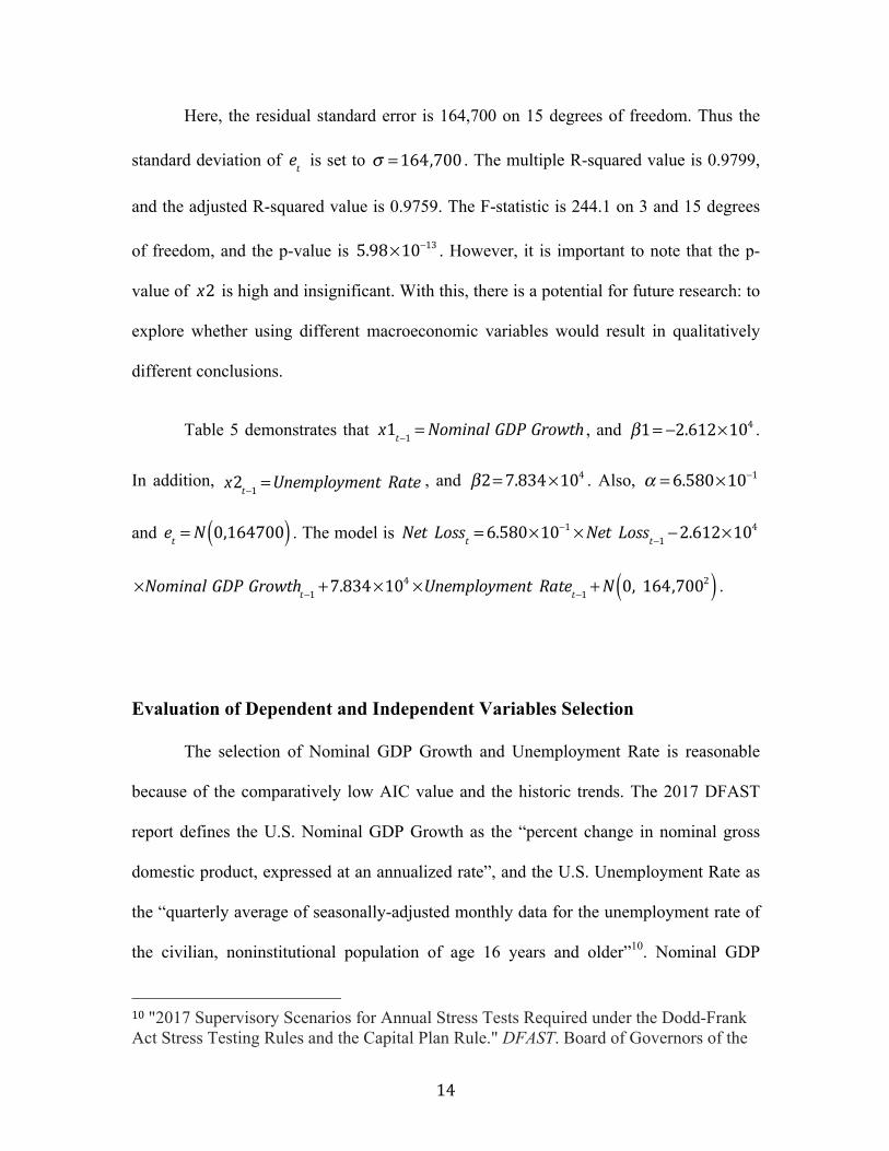
Here, the residual standard error is 164,700 on 15 degrees of freedom. Thus the

standard deviation of et is set to σ =164,700 . The multiple R-squared value is 0.9799,

and the adjusted R-squared value is 0.9759. The F-statistic is 244.1 on 3 and 15 degrees

of freedom, and the p-value is 5.98×10−13 . However, it is important to note that the p-

value of x2 is high and insignificant. With this, there is a potential for future research: to

explore whether using different macroeconomic variables would result in qualitatively

different conclusions.

Table 5 demonstrates that x1t−1 =Nominal GDP Growth , and β1= −2.612×104 .

In addition, x2t−1 =Unemployment Rate , and β2=7.834×104 . Also, α =6.580×10−1

and et =N 0,164700( ) . The model is Net Losst =6.580×10−1 ×Net Loss

t−1 −2.612×104

×Nominal GDP Growtht−1 +7.834×104 ×Unemployment Rate

t−1 +N 0,164,7002( ) .

Evaluation of Dependent and Independent Variables Selection

The selection of Nominal GDP Growth and Unemployment Rate is reasonable

because of the comparatively low AIC value and the historic trends. The 2017 DFAST

report defines the U.S. Nominal GDP Growth as the “percent change in nominal gross

domestic product, expressed at an annualized rate”, and the U.S. Unemployment Rate as

the “quarterly average of seasonally-adjusted monthly data for the unemployment rate of

the civilian, noninstitutional population of age 16 years and older”10. Nominal GDP

10"2017 Supervisory Scenarios for Annual Stress Tests Required under the Dodd-Frank Act Stress Testing Rules and the Capital Plan Rule." DFAST. Board of Governors of the

15

Growth is assigned a negative correlation with Yt , because when nominal GDP growth

increases, the nation as a whole has more money to spend, which means that the average

individual has more money to spend. This means that they are less likely to default on

their loans, which results in a decrease in the net loss on loans and leases of Bank of

America. Unlike Nominal GDP Growth, Unemployment Rate is assigned a positive

correlation with Yt , because when the unemployment rate increases, there are generally

more people lacking an income, who are more likely to be taking out loans and defaulting

on them. This means that an increase in unemployment rate results in the net loss on

loans and leases of Bank of America increasing as well.

The selection of the product of Net Loss to Average Total LN & LS of Bank of

America and Net Loans and Leases as a dependent variable is also beneficial as Y

captures the product of the net loss of the loans and leases and the value of the portfolio.

The values of the variable Y are historically negatively and positively correlated with

Nominal GDP Growth and Unemployment Rate respectively. They are being used as

possible definitions of default.

Furthermore, the focus is on the net loss value of a single large bank, rather than

on a blended dataset of a group of banks, to avoid introducing unnecessary uncontrollable

or immeasurable factors, such as ensuring that the net losses of all of those banks follow

a similar enough trend that they can be aggregated into one dataset. Bank of America, in

particular, is chosen, because it is one of the ten largest banks in terms of market

capitalization (it is the fourth largest globally, and third largest in the US after JP Morgan

Federal Reserve System, 2017. Web. 7 Apr. 2017. <https://www.federalreserve.gov/newsevents/pressreleases/files/bcreg20170203a5.pdf>.

16

Chase & Co and Wells Fargo & Co) and in January 2017, its market capitalization is

estimated to be $228.778 billion11.

Assumptions and limitations

It is important to recognize assumptions that are made in the model creation

process. An important assumption being made is that net loss is not driving or affecting

the macroeconomic variables. Rather, the assumption that the macroeconomic variables

impact the net loss is being modeled.

Additionally, a limitation of this exploration is that combinations of

macroeconomic variables shifted by one, two or even more quarterly time intervals are

not being considered. The fit of the macroeconomic variables is based on how the

Nominal GDP Growth at time t −1 and the Unemployment Rate at time t −1 interact

with Yt−1 and with one another. It is possible that combining different macroeconomic

variables at, for example, time t −1 and time t −2 , could create a fit with a lower

residual standard error. Yet such a shift would also result in the loss of one or more data

points (similar to exploring AR(2) or AR(3) models), and perhaps result in over-fitting.

Nonetheless, although the chosen macroeconomic variables may not result in the

absolutely best combination (with the lowest AIC value), the focus of this exploration is

on the application of the model in Monte Carlo simulations.

11 "World's Largest Banks 2017." Banks around the World. N.p., 2017. Web. 07 Apr. 2017. <http://www.relbanks.com/worlds-top-banks/market-cap>.

17

Additional assumptions are made regarding the historic dataset utilized in the

creation of the model. The dataset consists of only 18 observations: 18 consecutive data

points of quarterly data extracted primarily from the 2017 DFAST report (for the

independent variables) and the FFIEC report (for the dependent variable). It is being

assumed that this dataset accurately and comprehensively captures the relationships

between the independent variables and dependent variable of future scenarios, and that

over-fitting is not occurring. Furthermore, the dataset is assumed to capture expected,

baseline data in an environment where the independent variables are predictable and

normal, and the dependent variable also does not exhibit effects of an abnormal. These

are significant assumptions, and, moving forward, assessing whether these assumptions

are valid could be addressed by someone in future research. That said, the limitation on

the size of the available dataset is challenging to overcome in any meaningful way.

Finally, it is also important to note that the macroeconomic data used when

selecting the most favorable combination of macroeconomic variables is not identical to

the macroeconomic data, which will be used in the Monte Carlo simulations. This is

because the Monte Carlo simulations will be performed on future quarters with

nonexistent net loss data. Nonetheless, the focus of the exploration is not the selection of

the macroeconomic variables, but the Monte Carlo simulations performed on the AR(1)

model built by using them.

18

Monte Carlo Simulations

AR(1) Model

An autoregressive model of order 1 (AR(1)) is a time series model in which the

order refers to the number of time units into the past for which variables are used to

predict one step into the future using a linear predictor. The general form of the AR(1)

model being applied here is: Yt =αYt−1 +β1x1t−1 +β2x2t−1 +et .

Although x1t−1 and x2t−1 involve indexes explaining that they too refer to the

previous quarter’s value, both β1 and β2 , and x1t−1 and x2t−1 serve as constants in this

equation. After all, the fixed values for α , β1 and β2 for the Nominal GDP Growth and

the Unemployment Rate have been determined. The values for the Nominal GDP Growth

and Unemployment Rate under all three scenarios are deterministic values, as they are

determined by the DFAST 2017 report. Their evolution is deterministic, rather than

random, as it is based on real data and determined deliberately. The multiplication of the

fixed coefficient values by the fixed macroeconomic variable values results in the term

β1x1t−1 +β2x2t−1 serving as a constant.

19

Residual

The final part of the AR(1) model, Yt =αYt−1 +β1x1t−1 +β2x2t−1 +et , is the shock,

which is taken to be a normally distributed random variable with a mean of 0 and

standard deviation σ . For a fixed value of σ , the value of the innovation is stochastic

and varies over realizations. It is important for the mathematical formulation, since it is

the part that cannot be reasoned out and guessed in advance: it is the discrepancy between

the expected, real-value results and the simulated values. Thus for the three different

scenarios and therefore also differing values of the Nominal GDP Growth and the

Unemployment Rate, there are varying, randomly generated values for the shock. The

standard deviation is fixed at σ =164,700 . Therefore, while the evolution of the

macroeconomic variables is deterministic, as the shock is a normally distributed random

variable, σ is constant while the shock is not.

For smaller values of σ , the changes between Yt values is estimated to be

smaller, since there is less randomness involved with the generation of such Yt values.

This will be confirmed later using Monte Carlo simulations. Similarly, it is also expected

that later quarters of Yt that are simulated using Monte Carlo simulations show higher

degrees of variability as the shocks accumulate. This is because later values involve both

that quarter’s shock, in addition to the earlier quarters’ shocks. As established previously,

β1x1t−1 +β2x2t−1 serves as a predictable constant that can be calculated. Let

ct−1 = β1x1t−1 +β2x2t−1 , and so the estimations of Y1 , Y2 and Y3 are:

20

Y1 =αY0 + c0 +e1Y2 =αY1 + c1 +e2Y2 =α αY0 + c0 +e1( )+ c1 +e2Y2 =α

2Y0 +αc0 + c1 +αe1 +e2Y3 =αY2 + c2 +e3Y3 =α α 2Y0 +αc0 +αe1 + c1 +e2( )+ c2 +e3Y3 =α

3Y0 +α2c0 +αc1 + c2 +α

2e1 +αe2 +e3

Thus later quarters are expected to show the highest degrees of variability due to

the addition of further residual terms.

Data under the three Scenarios

For the Monte Carlo simulation, three different scenarios will be explored – with

fixed values of α , β1 and β2 according to the previous findings, in addition to the

value of σ , the standard deviation of the shock. The data of the Nominal GDP Growth

and the Unemployment Rate to be used for the Monte Carlo simulations span September

2016 (Q3 2016) until March 2020 (Q1 2020) and are extracted from the DFAST 2017

report. The scenarios capture the values of the 2017 DFAST report’s estimated Baseline

scenario, their Adverse scenario and their Severely Adverse scenario – which are labels

given to the values of the macroeconomic variables based on their unlikeliness and the

powerful negative impact they are assumed to have on the economy and therefore also on

banks’ net losses. Thus this data for the Nominal GDP Growth and the Unemployment

Rate can be used in combination with the actual data of Yt and Yt−1 to create the Monte

21

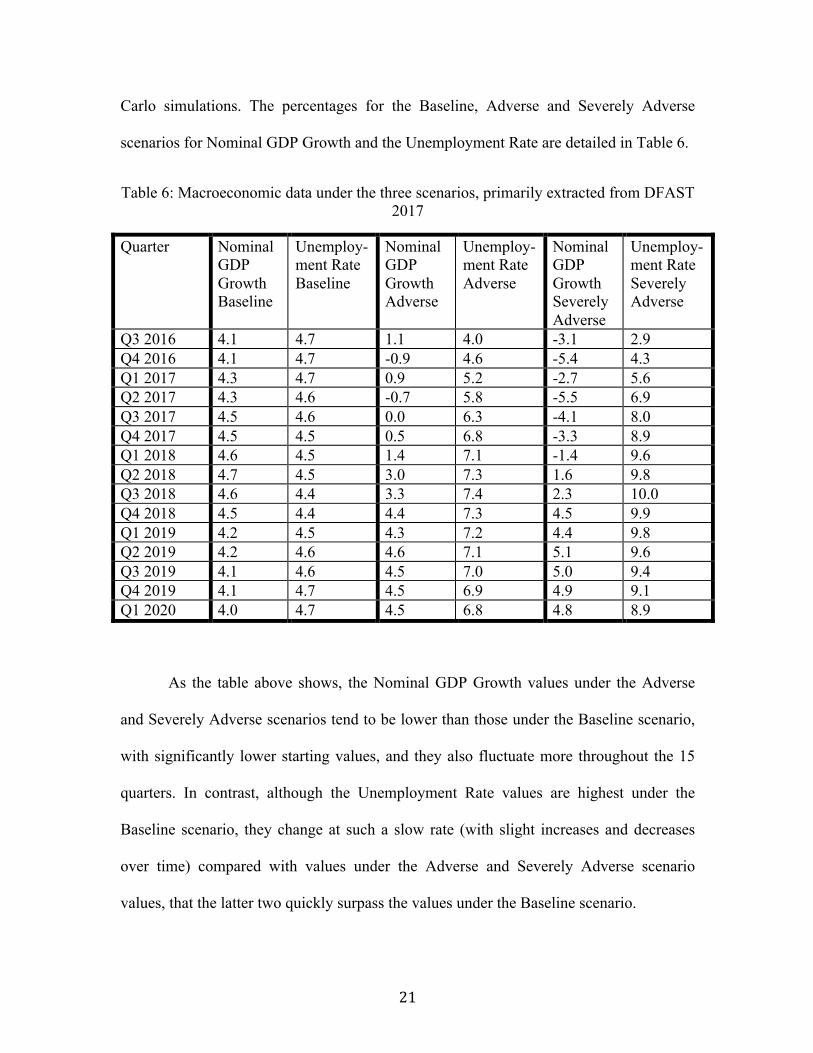
Carlo simulations. The percentages for the Baseline, Adverse and Severely Adverse

scenarios for Nominal GDP Growth and the Unemployment Rate are detailed in Table 6.

Table 6: Macroeconomic data under the three scenarios, primarily extracted from DFAST 2017

Quarter Nominal GDP Growth Baseline

Unemploy-ment Rate Baseline

Nominal GDP Growth Adverse

Unemploy-ment Rate Adverse

Nominal GDP Growth Severely Adverse

Unemploy-ment Rate Severely Adverse

Q3 2016 4.1 4.7 1.1 4.0 -3.1 2.9 Q4 2016 4.1 4.7 -0.9 4.6 -5.4 4.3 Q1 2017 4.3 4.7 0.9 5.2 -2.7 5.6 Q2 2017 4.3 4.6 -0.7 5.8 -5.5 6.9 Q3 2017 4.5 4.6 0.0 6.3 -4.1 8.0 Q4 2017 4.5 4.5 0.5 6.8 -3.3 8.9 Q1 2018 4.6 4.5 1.4 7.1 -1.4 9.6 Q2 2018 4.7 4.5 3.0 7.3 1.6 9.8 Q3 2018 4.6 4.4 3.3 7.4 2.3 10.0 Q4 2018 4.5 4.4 4.4 7.3 4.5 9.9 Q1 2019 4.2 4.5 4.3 7.2 4.4 9.8 Q2 2019 4.2 4.6 4.6 7.1 5.1 9.6 Q3 2019 4.1 4.6 4.5 7.0 5.0 9.4 Q4 2019 4.1 4.7 4.5 6.9 4.9 9.1 Q1 2020 4.0 4.7 4.5 6.8 4.8 8.9

As the table above shows, the Nominal GDP Growth values under the Adverse

and Severely Adverse scenarios tend to be lower than those under the Baseline scenario,

with significantly lower starting values, and they also fluctuate more throughout the 15

quarters. In contrast, although the Unemployment Rate values are highest under the

Baseline scenario, they change at such a slow rate (with slight increases and decreases

over time) compared with values under the Adverse and Severely Adverse scenario

values, that the latter two quickly surpass the values under the Baseline scenario.

22

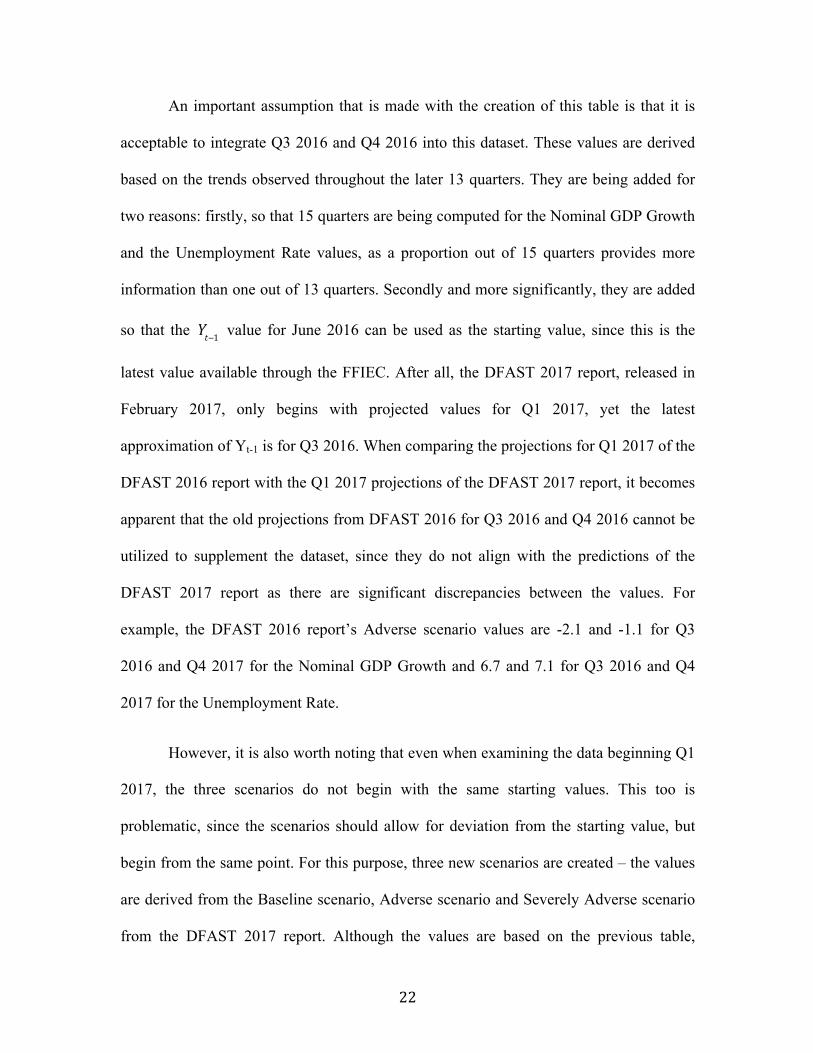
An important assumption that is made with the creation of this table is that it is

acceptable to integrate Q3 2016 and Q4 2016 into this dataset. These values are derived

based on the trends observed throughout the later 13 quarters. They are being added for

two reasons: firstly, so that 15 quarters are being computed for the Nominal GDP Growth

and the Unemployment Rate values, as a proportion out of 15 quarters provides more

information than one out of 13 quarters. Secondly and more significantly, they are added

so that the Yt−1 value for June 2016 can be used as the starting value, since this is the

latest value available through the FFIEC. After all, the DFAST 2017 report, released in

February 2017, only begins with projected values for Q1 2017, yet the latest

approximation of Yt-1 is for Q3 2016. When comparing the projections for Q1 2017 of the

DFAST 2016 report with the Q1 2017 projections of the DFAST 2017 report, it becomes

apparent that the old projections from DFAST 2016 for Q3 2016 and Q4 2016 cannot be

utilized to supplement the dataset, since they do not align with the predictions of the

DFAST 2017 report as there are significant discrepancies between the values. For

example, the DFAST 2016 report’s Adverse scenario values are -2.1 and -1.1 for Q3

2016 and Q4 2017 for the Nominal GDP Growth and 6.7 and 7.1 for Q3 2016 and Q4

2017 for the Unemployment Rate.

However, it is also worth noting that even when examining the data beginning Q1

2017, the three scenarios do not begin with the same starting values. This too is

problematic, since the scenarios should allow for deviation from the starting value, but

begin from the same point. For this purpose, three new scenarios are created – the values

are derived from the Baseline scenario, Adverse scenario and Severely Adverse scenario

from the DFAST 2017 report. Although the values are based on the previous table,

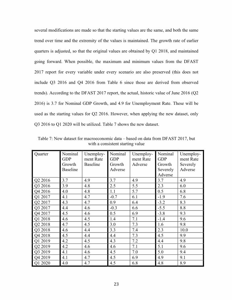
23

several modifications are made so that the starting values are the same, and both the same

trend over time and the extremity of the values is maintained. The growth rate of earlier

quarters is adjusted, so that the original values are obtained by Q1 2018, and maintained

going forward. When possible, the maximum and minimum values from the DFAST

2017 report for every variable under every scenario are also preserved (this does not

include Q3 2016 and Q4 2016 from Table 6 since those are derived from observed

trends). According to the DFAST 2017 report, the actual, historic value of June 2016 (Q2

2016) is 3.7 for Nominal GDP Growth, and 4.9 for Unemployment Rate. These will be

used as the starting values for Q2 2016. However, when applying the new dataset, only

Q3 2016 to Q1 2020 will be utilized. Table 7 shows the new dataset.

Table 7: New dataset for macroeconomic data – based on data from DFAST 2017, but with a consistent starting value

Quarter Nominal GDP Growth Baseline

Unemploy-ment Rate Baseline

Nominal GDP Growth Adverse

Unemploy-ment Rate Adverse

Nominal GDP Growth Severely Adverse

Unemploy-ment Rate Severely Adverse

Q2 2016 3.7 4.9 3.7 4.9 3.7 4.9 Q3 2016 3.9 4.8 2.5 5.5 2.3 6.0 Q4 2016 4.0 4.8 1.1 5.7 0.5 6.8 Q1 2017 4.1 4.7 -0.7 6.1 -1.9 7.6 Q2 2017 4.3 4.7 0.9 6.4 -3.2 8.3 Q3 2017 4.4 4.6 -0.3 6.6 -5.5 8.8 Q4 2017 4.5 4.6 0.5 6.9 -3.8 9.3 Q1 2018 4.6 4.5 1.4 7.1 -1.4 9.6 Q2 2018 4.7 4.5 3.0 7.3 1.6 9.8 Q3 2018 4.6 4.4 3.3 7.4 2.3 10.0 Q4 2018 4.5 4.4 4.4 7.3 4.5 9.9 Q1 2019 4.2 4.5 4.3 7.2 4.4 9.8 Q2 2019 4.2 4.6 4.6 7.1 5.1 9.6 Q3 2019 4.1 4.6 4.5 7.0 5.0 9.4 Q4 2019 4.1 4.7 4.5 6.9 4.9 9.1 Q1 2020 4.0 4.7 4.5 6.8 4.8 8.9

24

Going forward, this new dataset, which is based on the previous dataset with

modifications made to account for having the same Q2 2016 value, will be used in the

Monte Carlo simulations.

Realizations – 15 Quarters of Simulated Data

Rather than calculating the value of Y for 18 quarters from Q1 2003 until Q2

2007, for this simulation, 15 future quarters are being evaluated. This covers the range of

data from Q3 2016 until Q1 2020. This means that calculations for the combination of the

Nominal GDP Growth values, the Unemployment Rate values and the values of the

shock’s standard deviation σ , actually occur 15 times, because 15 quarters are projected.

However, as datasets are created through the simulation, only one actual value of Yt−1 is

needed – the starting value of September 2016, as each future quarters’ values of Yt−1 are

taken from the previous quarters’ Y result.

Each realization is a set of 15 quarters beginning with the starting Yt−1 value for

Q3 2016 and ending with a computed result for Yt for Q1 2020 for each combination of

the Nominal GDP Growth, the Unemployment Rate and σ . Several tests will be

performed on each realization as a whole in later sections – documenting whether a

certain outcome occurred throughout the realization. This will be elaborated upon in the

following section, but for the time being, it is important to recognize that this exploration

results in the creation of datasets utilizing constants for independent variables derived

from real data in an attempt to accurately predict the net loss for future quarters.

25

10,000 Trials for the Monte Carlo Simulations

The above calculations for every combination of the Nominal GDP Growth, the

Unemployment Rate and σ are repeated for a total of 10,000 trials for each under the

three scenarios. This means that every realization, in addition to how its outcome in

specific tests performed on it, is computed 10,000 times under the three scenarios and

combinations of the Nominal GDP Growth, the Unemployment Rate and σ .

Applying this time series model to create datasets is the logic behind Monte Carlo

simulations. Monte Carlo simulations involve an iterative process of repeating a

computation, which includes randomness, thousands of times and then estimating the

probabilities associated with outcomes. It results in a pseudo-random independent and

identically distributed sequence of realizations of Bernoulli trials representing whether a

certain outcome occurred in a given realization. Monte Carlo simulations are being used

to address questions about the probabilities of success of Bernoulli trials and the

probabilities of outcomes, which are explored through the analysis in the following

section.

Additional Considerations

Throughout the building of the financial risk model and the Monte Carlo

simulations, simplifying assumptions are made, as the focus of this exploration is on the

application of the model in the Monte Carlo simulations. Such assumptions include that

Yt can be determined from the Nominal GDP Growth and Unemployment Rate.

26

Several assumptions are made with regard to determining the type of model: an

AR(1) model, which depends on two macroeconomic variables (in addition to the shocks

and Yt−1 , as implied by the AR(1) structure). Perhaps an AR(2) model could provide an

alternative fit, but this is not explored, as an additional one out of the 18 historic data

points would be forfeited for this. A combination of exactly two macroeconomic

variables, with predetermined signs, is selected; and thus an assumption is that these

limiting factors still result in an accurate prediction without over-fitting the model. An

additional assumption implied through the choice of the AR(1) model is that the

coefficients of the macroeconomic variables (β1 and β2) and standard deviation of

stocks do not change over time. The shocks are also assumed to be independent random

shocks, which follow a normal distribution, and it is assumed that there is no

autocorrelation among them. Additionally, residuals are assumed to have stationarity,

which means that they are assumed to have a constant mean and variance.

27

What If Analysis

Analyses

Having explored the creation of the simulated dataset, a variety of analyses can be

performed on it. Through the Threshold Analysis, it is being documented whether, in any

of the trials, a certain anticipated outcome occurs, regardless of how many quarters the

outcome occurs in. There are also specific analyses capturing whether a certain outcome

occurs more than five or ten times, or within the first five or ten quarters. In the Statistical

Analysis, a variety of statistics are being calculated from the dataset, and the results are

captured in charts or tables. All of the charts are color-coded in the same way: blue

represents the outcome under the Baseline scenario, green captures the outcome under the

Adverse scenario and red shows the outcome under the Severely Adverse scenario. It

would be a simple matter to provide confidence intervals for the probabilities in the

figures that follow. However, these intervals would be so narrow as to not be of much

interest.

Threshold Analysis

Through six distinct net loss outcomes, it is measured in how many realizations a

certain outcome occurs for each of the scenarios. Several thresholds, which are

percentages of the starting Yt-1 value of $4,039,752.2, are used to compare the scenarios.

28

Figure 1: Estimated probability that the net loss value falls below a given percentage of the starting net loss value in at least one of the quarters

Figure 2: Estimated probability that the net loss value exceeds a given percentage of the starting net loss value in at least one of the quarters

29

Figure 1 shows that the minimum values of net loss under the Baseline scenario

are lower than those of the Adverse scenario, and significantly lower than under the

Severely Adverse scenario. Figure 2 demonstrates a similar outcome: the maximum

values under the Baseline scenario tend to surpass a higher threshold value compared

with the values under the Adverse and Severely Adverse scenarios. However, the

discrepancy between the values under the Baseline and Severely Adverse scenarios is

more drastic in Figure 1 compared with Figure 2. Figure 2 has more significant impacts

in the real world, as it captures when the net loss exceeds particular high thresholds,

which is very important for stakeholders to know (compared with instances when the net

loss is particularly low). For this reason, further exploration is conducted on the ways in

which high thresholds are exceeded.

Figure 3: Estimated probability that the net loss value exceeds a given percentage of the starting net loss value in at least five of the fifteen quarters

30

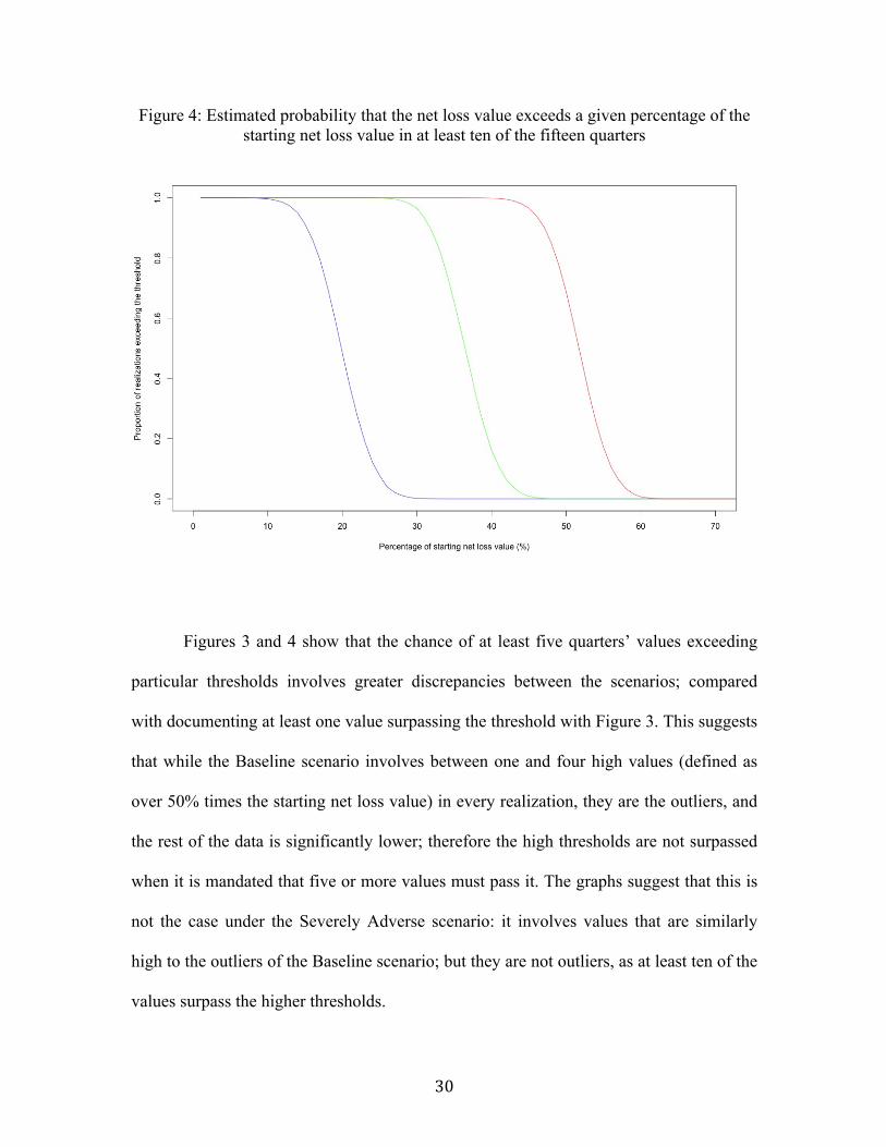
Figure 4: Estimated probability that the net loss value exceeds a given percentage of the starting net loss value in at least ten of the fifteen quarters

Figures 3 and 4 show that the chance of at least five quarters’ values exceeding

particular thresholds involves greater discrepancies between the scenarios; compared

with documenting at least one value surpassing the threshold with Figure 3. This suggests

that while the Baseline scenario involves between one and four high values (defined as

over 50% times the starting net loss value) in every realization, they are the outliers, and

the rest of the data is significantly lower; therefore the high thresholds are not surpassed

when it is mandated that five or more values must pass it. The graphs suggest that this is

not the case under the Severely Adverse scenario: it involves values that are similarly

high to the outliers of the Baseline scenario; but they are not outliers, as at least ten of the

values surpass the higher thresholds.

31

Additionally, in Figure 2, the change is less immediate; it covers a range of about

25% for the values to change from surpassing the thresholds to not surpassing the

thresholds. The shock accounts for a lot of fluctuation in whether or not the condition is

met. By comparison, in both Figures 3 and 4, the change occurs over a span of about

15%; it is more clear-cut whether five or ten of the fifteen quarters exceed a certain

threshold, and less dependent on the residual.

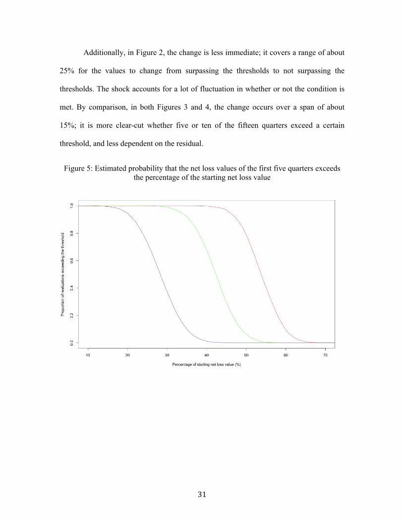
Figure 5: Estimated probability that the net loss values of the first five quarters exceeds the percentage of the starting net loss value

32

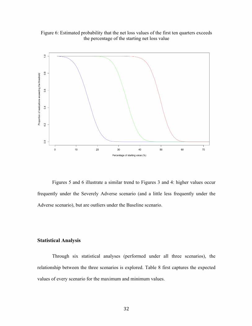
Figure 6: Estimated probability that the net loss values of the first ten quarters exceeds the percentage of the starting net loss value

Figures 5 and 6 illustrate a similar trend to Figures 3 and 4: higher values occur

frequently under the Severely Adverse scenario (and a little less frequently under the

Adverse scenario), but are outliers under the Baseline scenario.

Statistical Analysis

Through six statistical analyses (performed under all three scenarios), the

relationship between the three scenarios is explored. Table 8 first captures the expected

values of every scenario for the maximum and minimum values.

33

Table 8: Expected values of the minimum and maximum values under each scenario

Baseline Scenario ($)

Adverse Scenario ($)

Severely Adverse Scenario ($)

Expected Value of Minimum 504,546 1,125,670 1,681,405 Expected Value of Maximum 2,933,024 3,019,828 3,066,457

As Table 8 shows, the discrepancy between the minimum values under the

scenarios is drastic: the minimum value under the Adverse scenario is more than 220% of

the minimum value under the Baseline scenario (a difference of $621,124). By contrast,

the difference between the expected value of the maximum under the Baseline scenario

compared with the minimum value under the Adverse scenario is less than 103% of the

value, with a difference of only $86,804. A similar pattern is also observed with values

under the Severely Adverse scenario.

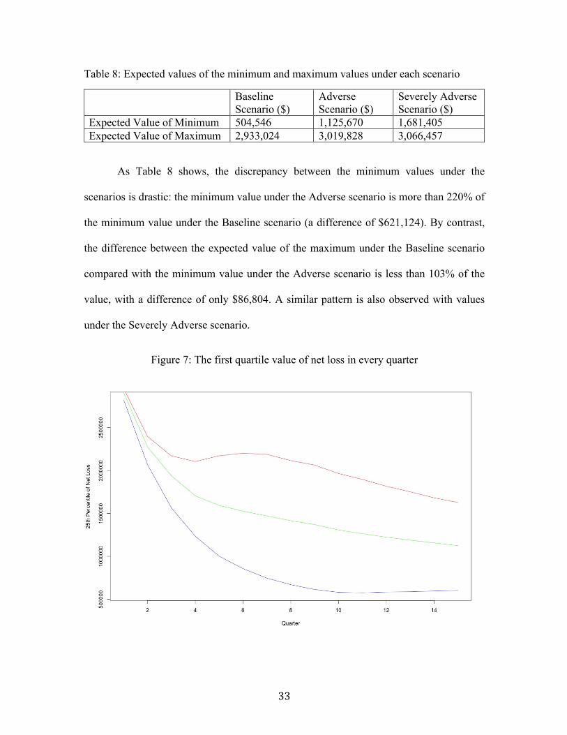
Figure 7: The first quartile value of net loss in every quarter

34

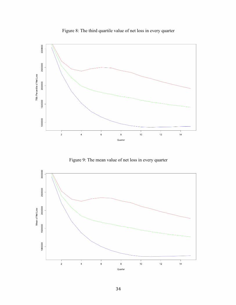
Figure 8: The third quartile value of net loss in every quarter

Figure 9: The mean value of net loss in every quarter

35

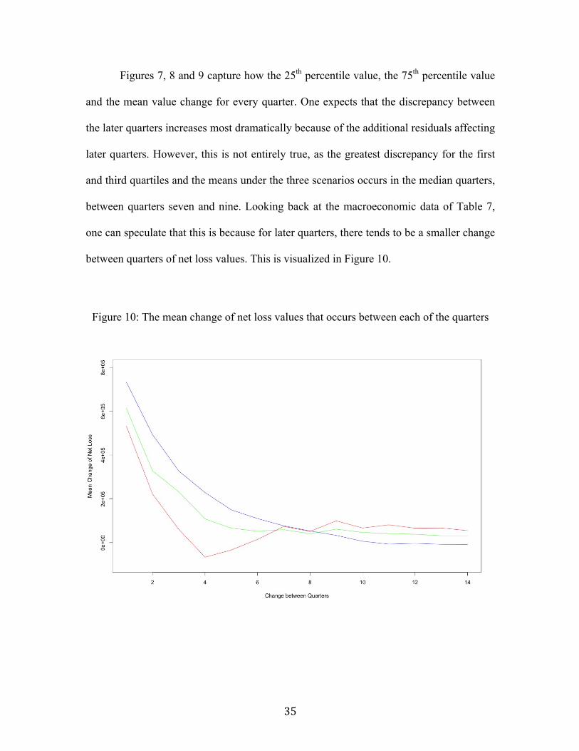
Figures 7, 8 and 9 capture how the 25th percentile value, the 75th percentile value

and the mean value change for every quarter. One expects that the discrepancy between

the later quarters increases most dramatically because of the additional residuals affecting

later quarters. However, this is not entirely true, as the greatest discrepancy for the first

and third quartiles and the means under the three scenarios occurs in the median quarters,

between quarters seven and nine. Looking back at the macroeconomic data of Table 7,

one can speculate that this is because for later quarters, there tends to be a smaller change

between quarters of net loss values. This is visualized in Figure 10.

Figure 10: The mean change of net loss values that occurs between each of the quarters

36

Figure 10 captures the change of net loss between the quarters. It is important to

note that the net loss tends to decrease over the time periods, and thus the graph

demonstrates quartert – quartert+1, rather than quartert+1 – quartert. Also, in early quarters,

the change is greatest for values under the Baseline scenario, as the net loss value

decreases. Yet by the later quarters, the change is greatest for values under the Severely

Adverse scenario.

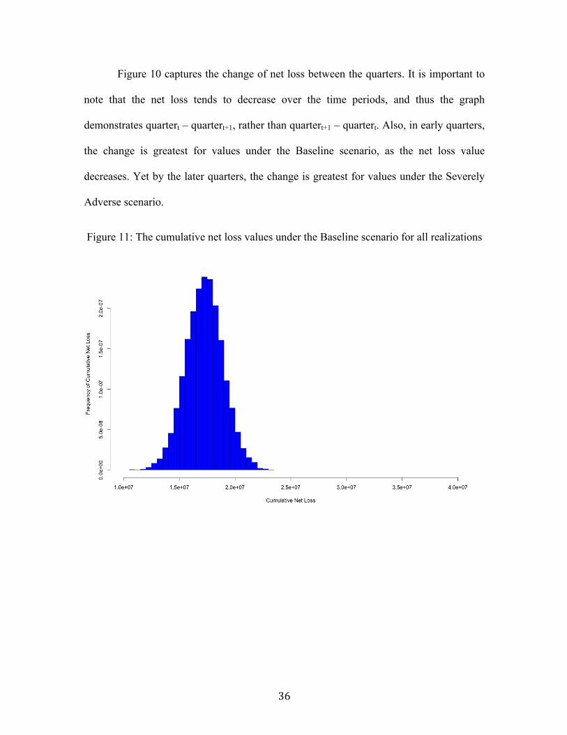
Figure 11: The cumulative net loss values under the Baseline scenario for all realizations

37

Figure 12: The cumulative net loss values under the Adverse scenario for all realizations

Figure 13: The cumulative net loss values under the Severely Adverse scenario for all realizations

38

Figures 11, 12 and 13 demonstrate the cumulative net loss values for all

realizations of the Monte Carlo simulation under each of the scenarios. The x-axes of the

histograms are kept constant to demonstrate the discrepancy between the cumulative net

losses under the three scenarios. Although the expected value of the cumulative net loss

under each of the scenarios is very different, there is some overlap between the

cumulative net loss values under the Adverse scenario with values under the Severely

Adverse scenario and under the Baseline scenario. This demonstrates the impact of the

randomness of the residuals, as there is still a probabilistic chance that, under Adverse

macroeconomic conditions, the cumulative net loss could behave as though it is under the

Baseline scenario or under the Severely Adverse scenario. The following figures further

explore the impact of the randomness of the residuals by using different variances.

Figure 14: How changing the variance of the residuals affects the first and third quartiles under the Baseline scenario

39

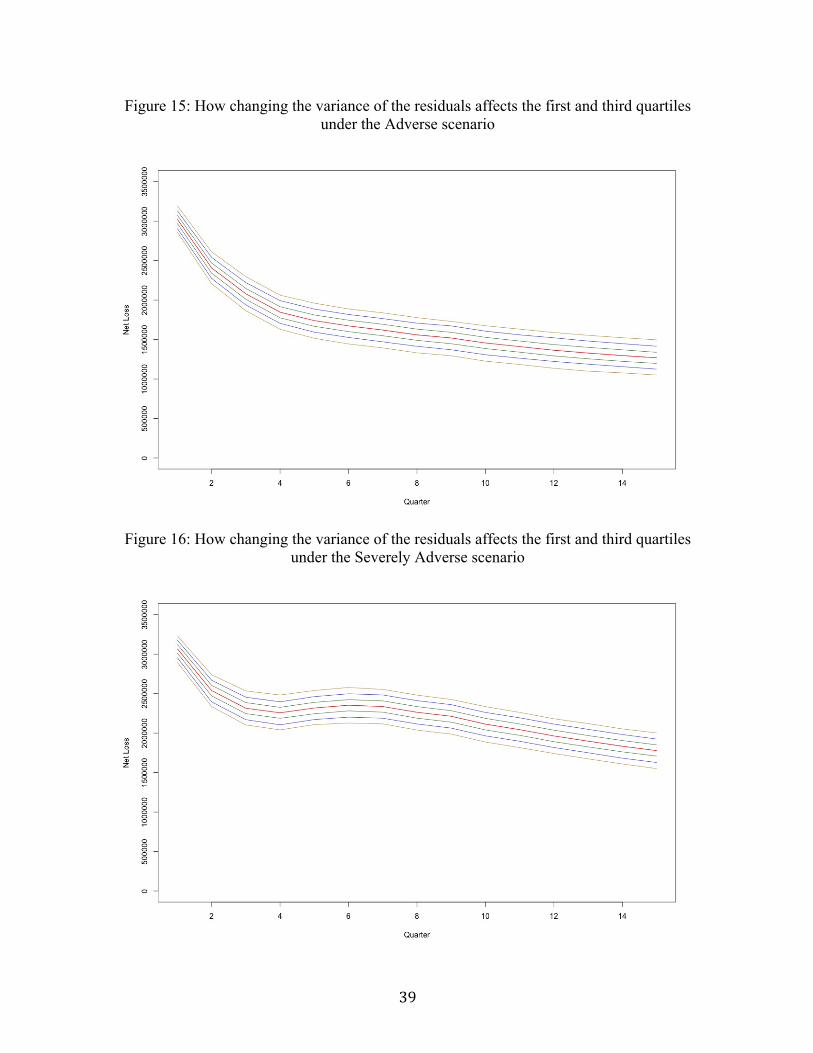
Figure 15: How changing the variance of the residuals affects the first and third quartiles under the Adverse scenario

Figure 16: How changing the variance of the residuals affects the first and third quartiles under the Severely Adverse scenario

40

Figures 14, 15 and 16 capture the impact that changing the variance of the

residuals has on the first and third quartile values for each of the quarters under the three

scenarios. In terms of color-coding, red indicates the 25th and 75th percentile values for

σ =0 . As one might predict, for , the 25th and 75th percentiles are green, for

σ =164,700 , the 25th and 75th percentiles are blue, and for , the 25th and

75th percentiles are brown. As the variance increases, the discrepancy between the 25th

and 75th percentiles under each of the scenarios also increases. The change in discrepancy

between the 25th and 75th percentiles caused by the increase in the variance is slightly

more apparent under the Severely Adverse scenario – as the increased randomness has

the greatest impact on higher net loss values. Finally, when comparing the effect of

changing the variance under the three scenarios, it is clear that the trend of the net loss

throughout the fifteen quarters remains the same for all of the variance values.

σ =80,000

σ =250,000

41

Conclusion

Summary

In this exploration, the patterns observed under the Baseline, Adverse and

Severely Adverse scenarios are investigated through the Monte Carlo simulations. The

cumulative net loss experiences great variation under the three scenarios, although there

is still some probabilistic overlap between the Adverse and Baseline scenarios, and

Adverse and Severely Adverse scenarios. While it is expected that the residuals result in

the mean net loss of the latest quarters having the greatest discrepancy between the three

scenarios, the greatest discrepancy occurs with median quarters. Furthermore, the three

scenarios result in very similar outcomes when documenting whether any one of the

fifteen quarters per realization surpasses a specific threshold. Yet when assessing whether

at least five of the fifteen quarters per realization surpass a given threshold, there is a

significant discrepancy between the three curves as the high net loss values occur more

frequently under the Severely Adverse scenario, but are outliers under the Baseline

scenario.

Future opportunities for research

In terms of future opportunities for research, it is important to remember that there

are other threshold analyses and statistical estimations, which can be performed on the

datasets.

42

Similarly, there are also other questions to be explored regarding the stakeholders,

such as: What happens if the stock markets plummet by 50%, and how does this affect

the macroeconomic variables, and by extension, net loss, over time? How are individuals

affected by abrupt increases in net loss – and who is most likely to be affected? As

macroeconomic factors change, how does a specific individual’s probability of default

change?

Verifying some of the assumptions made in the model creation process – such as

autocorrelation or stationarity – could also be fruitful.

Applications

In terms of further applications, an additional consideration is the economic

background beyond the dependent variable and the two chosen macroeconomic variables.

Another financial risk model could be constructed based on a different combination of

macroeconomic variables, perhaps expanding beyond the current selection of 18. This

model need not be applied to calculating net loss on loans and leases of Bank of America;

other dependent variables and institutions could be explored. For example the sizes of

portfolios, various types of revenues, or various types of expenses could also be

investigated and estimated through a time series model and Monte Carlo simulations.

43

Variables and Abbreviations

Baseline Scenario of normal, expected macroeconomic conditions

Adverse Scenario of abnormal macroeconomic conditions

Severely Adverse Scenario of very abnormal, unexpected macroeconomic conditions

AR(1) First-order autoregressive model

Yt Net loss on loans and leases for Bank of America

α Alpha, the coefficient of Yt−1

Yt−1 Net loss on loans and leases for Bank of America, of the previous quarter

β1 Coefficient of x1t−1

x1t−1 First macroeconomic variable, of the previous quarter

β2 Coefficient of x2t−1

x2t−1 Second macroeconomic variable, of the previous quarter

et Residual

PPNR Pre Provision Net Revenue

CCAR Comprehensive Capital Analysis and Review

DFAST Dodd-Frank Act Stress Test

Realization Set of 15 quarters of simulated data

σ Standard deviation of the residual

Q Quarter

FDIC Federal Deposit Insurance Corporation

FFIEC Federal Financial Institutions Examination Council

44

Appendices

Appendix 1: Macroeconomic Variable Analysis

In this section, the code used to evaluate the optimal combination of the 18

macroeconomic variables with the lowest residual sum of squares is provided.

library(nnls) Yt_1 <- c(2617528, 1965774, 1805622, 1720196.352, 1524910.09, 1050805.284, 944571.8961, 760586.3874, 719641.7903, 551249.5814, 504741.536, 847467.7024, 875393.6768, 572299.422, 490419.1576, 556428.114, 634494.712, 834397.5627) RealGDPGrowth <- c(0.3, 2.1, 3.8, 6.9, 4.8, 2.3, 3, 3.7, 3.5, 4.3, 2.1, 3.4, 2.3, 4.9, 1.2, 0.4, 3.2, 0.2) NominalGDPGrowth <- c(2.4, 4.6, 5.1, 9.3, 6.8, 5.9, 6.6, 6.3, 6.4, 8.3, 5.1, 7.3, 5.4, 8.2, 4.5, 3.2, 4.6, 4.8) RealDisposableIncomeGrowth <- c(1.9, 1.1, 5.9, 6.7, 1.6, 2.9, 4, 2.1, 5.1, -3.8, 3.2, 2.1, 3.4, 9.5, 0.6, 1.2, 5.3, 2.6) NominalDisposableIncomeGrowth <- c(3.8, 4, 6.3, 9.3, 3.3, 6.1, 7, 4.5, 8.5, -1.8, 6, 6.6, 6.6, 11.5, 3.7, 4.1, 4.6, 6.5) UnemploymentRate <- c(5.9, 5.9, 6.1, 6.1, 5.8, 5.7, 5.6, 5.4, 5.4, 5.3, 5.1, 5, 5, 4.7, 4.6, 4.6, 4.4, 4.5) CPIInflationRate <- c(2.4, 4.2, -0.7, 3, 1.5, 3.4, 3.2, 2.6, 4.4, 2, 2.7, 6.2, 3.8, 2.1, 3.7, 3.8, -1.6, 4) ThreeMonthTreasuryRate <- c(1.3, 1.2, 1, 0.9, 0.9, 0.9, 1.1, 1.5, 2, 2.5, 2.9, 3.4, 3.8, 4.4, 4.7, 4.9, 4.9, 5) FiveYearTreasuryRate <- c(3.1, 2.9, 2.6, 3.1, 3.2, 3, 3.7, 3.5, 3.5, 3.9, 3.9, 4, 4.4, 4.6, 5, 4.8, 4.6, 4.6) TenYearTreasuryRate <- c(4.3, 4.2, 3.8, 4.4, 4.4, 4.1, 4.7, 4.4, 4.3, 4.4, 4.2, 4.3, 4.6, 4.7, 5.2, 5, 4.7, 4.8) BBBCorporateYield <- c(7.0, 6.5, 5.7, 6, 5.8, 5.5, 6.1, 5.8, 5.4, 5.4, 5.5, 5.5, 5.9, 6, 6.5, 6.4, 6.1, 6.1) MortgageRate <- c(6.1, 5.8, 5.5, 6.1, 5.9, 5.6, 6.2, 5.9, 5.7, 5.8, 5.7, 5.8, 6.2, 6.3, 6.6, 6.5, 6.2, 6.2) PrimeRate <- c(4.5, 4.3, 4.2, 4, 4, 4, 4, 4.4, 4.9, 5.4, 5.9, 6.4, 7 ,7.4 ,7.9, 8.3, 8.3, 8.3) DowJonesTotalStockMarketIndex <- c(8343.2, 8051.90, 9342.40, 9649.70, 10799.60, 11039.40, 11144.60, 10893.80, 11951.50, 11637.30, 11856.70, 12282.90, 12497.20, 13121.60, 12808.90, 13322.50, 14215.80, 14354.00) HousePriceIndex <- c(129, 134.1, 137, 141, 145.9, 151.6, 157.9, 163.2, 169.2, 177.1, 184.5, 190.2, 194.8, 198, 197.1, 195.8, 195.8, 193.3)

45

CommercialRealEstatePriceIndex <- c(142, 148, 149, 147, 146, 153, 160, 172, 176, 176, 182, 187, 195, 200, 209, 219, 217, 227) MarketVolatilityIndex <- c(42.6, 34.7, 29.1, 22.7, 21.1, 21.6, 20, 19.3, 16.6, 14.6, 17.7, 14.2, 16.5, 14.6, 23.8, 18.6, 12.7, 19.6) GrossNationalProduct <- c(11280.2, 11434.5, 11689.1, 11907.4, 12097.3, 12265.3, 12462.4, 12631.2, 12916.6, 13065.8, 13307.8, 13454.9, 13724.3, 13870.2, 13965.6, 14133.9, 14301.9, 14512.9) EffectiveFederalFundsRate <- c(1.24, 1.25, 1.22, 1.01, 0.98, 1.00, 1.03, 1.61, 2.16, 2.63, 3.04, 3.62, 4.16, 4.59, 4.99, 5.25, 5.24, 5.26) Yt <- c(1965774, 1805622, 1720196.352, 1524910.09, 1050805.284, 944571.8961, 760586.3874, 719641.7903, 551249.5814, 504741.536, 847467.7024, 875393.6768, 572299.422, 490419.1576, 556428.114, 634494.712, 834397.5627, 862906.9917) ones <- c(rep(0,18)) # Creating dataframe for macroeconomic variables df<-data.frame(Y=Yt,x0=Yt_1, x1=-RealGDPGrowth,x2=-NominalGDPGrowth,x3=-RealDisposableIncomeGrowth, x4=-NominalDisposableIncomeGrowth,x5=UnemploymentRate, x6=CPIInflationRate,x7=ThreeMonthTreasuryRate, x8=FiveYearTreasuryRate, x9=TenYearTreasuryRate, x10=BBBCorporateYield, x11=MortgageRate, x12=PrimeRate, x13=-DowJonesTotalStockMarketIndex, x14=-HousePriceIndex, x15=-CommercialRealEstatePriceIndex, x16=-MarketVolatilityIndex, x17=-GrossNationalProduct, x18=EffectiveFederalFundsRate) nm<-c("Yt","Yt_1", "RealGDPGrowth", "NominalGDPGrowth", "RealDisposableIncomeGrowth", "NominalDisposableIncomeGrowth", "UnemploymentRate", "CPIInflationRate", "ThreeMonthTreasuryRate", "FiveYearTreasuryRate", "TenYearTreasuryRate", "BBBCorporateYield", "MortgageRate", "PrimeRate", "DowJonesTotalStockMarketIndex", "HousePriceIndex", "CommercialRealEstatePriceIndex", "MarketVolatilityIndex", "GrossNationalProduct", "EffectiveFederalFundsRate") A<-matrix(c(df$x0,df$x1,df$x2),byrow=FALSE,ncol=3) A<-matrix(c(df[,2], df[,3],df[,4]),byrow=FALSE,ncol=3) b<-df$Y minrtssq<-99999999999999 for (i1 in 2) { for (i2 in (i1+1):20) { for (i3 in (i2+1):20) { if ((i1!=i2)&&(i2!=i3)&&(i2<=20)&&(i3<=20)) { print(c(i1,i2,i3))

46

A<-matrix(c(df[,i1], df[,i2],df[,i3]),byrow=FALSE,ncol=3) b<-df$Y NNLS<-nnls(A,b) beta<-NNLS$x nnz<-sum(beta>.000000001) if (nnz==3) { print(c(i1,i2,i3)) print(nm[c(i1,i2,i3)]) rtssq<-sqrt(sum(NNLS$res^2)) print(rtssq) print(NNLS$x) if (rtssq<minrtssq) { minrtssq<-rtssq m1<-i1 m2<-i2 m3<-i3 } } } } } } print(c(m1,m2,m3)) LM1<-lm(Y~0+x0+x2+x5,data=df) summary(LM1)

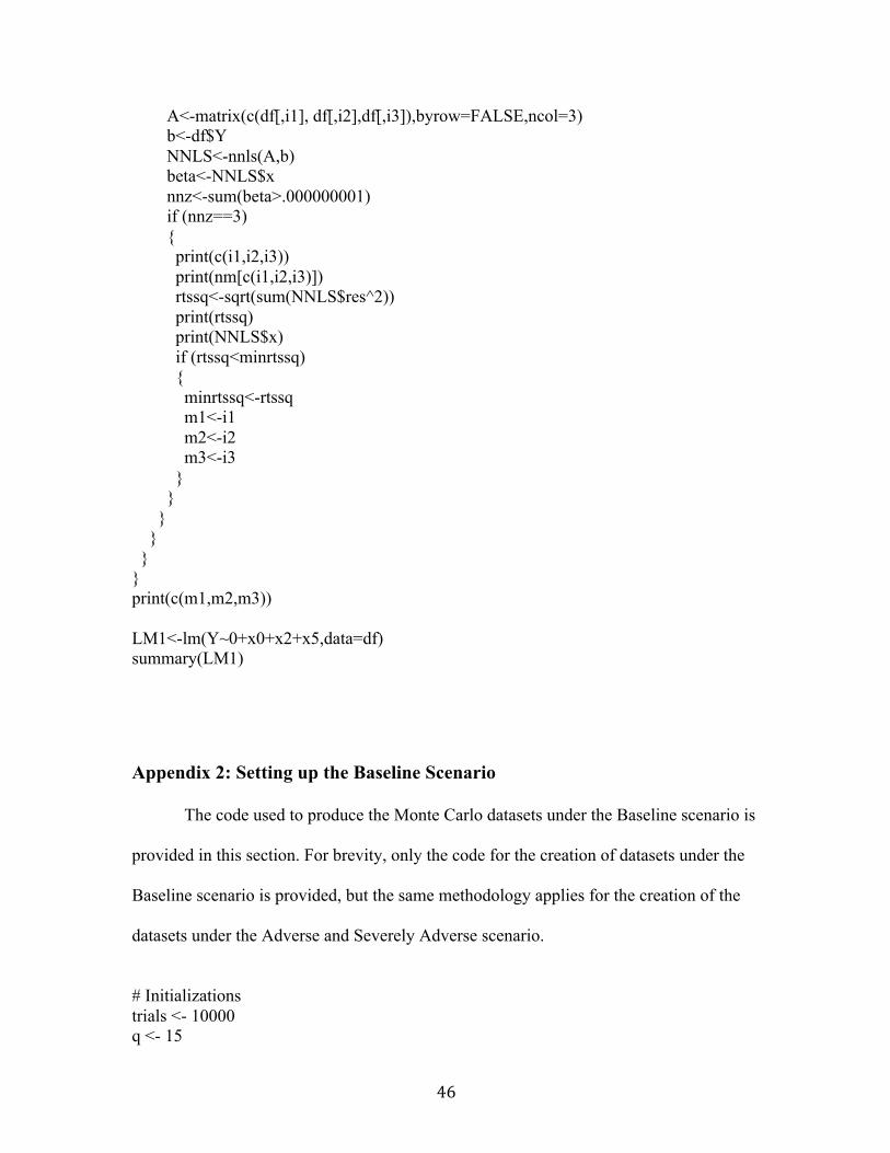
Appendix 2: Setting up the Baseline Scenario

The code used to produce the Monte Carlo datasets under the Baseline scenario is

provided in this section. For brevity, only the code for the creation of datasets under the

Baseline scenario is provided, but the same methodology applies for the creation of the

datasets under the Adverse and Severely Adverse scenario.

# Initializations trials <- 10000 q <- 15

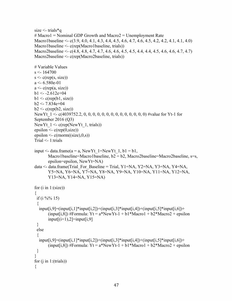
47

size <- trials*q # Macro1 = Nominal GDP Growth and Macro2 = Unemployment Rate Macro1baseline <- c(3.9, 4.0, 4.1, 4.3, 4.4, 4.5, 4.6, 4.7, 4.6, 4.5, 4.2, 4.2, 4.1, 4.1, 4.0) Macro1baseline <- c(rep(Macro1baseline, trials)) Macro2baseline <- c(4.8, 4.8, 4.7, 4.7, 4.6, 4.6, 4.5, 4.5, 4.4, 4.4, 4.5, 4.6, 4.6, 4.7, 4.7) Macro2baseline <- c(rep(Macro2baseline, trials)) # Variable Values s <- 164700 s <- c(rep(s, size)) a <- 6.580e-01 a <- c(rep(a, size)) b1 <- -2.612e+04 b1 <- c(rep(b1, size)) b2 <- 7.834e+04 b2 <- c(rep(b2, size)) NewYt_1 <- c(4039752.2, 0, 0, 0, 0, 0, 0, 0, 0, 0, 0, 0, 0, 0, 0) #value for Yt-1 for September 2016 (Q3) NewYt_1 <- c(rep(NewYt_1, trials)) epsilon <- c(rep(0,size)) epsilon <- c(rnorm((size),0,s)) Trial <- 1:trials input <- data.frame(a = a, NewYt_1=NewYt_1, b1 = b1, Macro1baseline=Macro1baseline, b2 = b2, Macro2baseline=Macro2baseline, s=s, epsilon=epsilon, NewYt=NA) data <- data.frame(Trial_For_Baseline = Trial, Y1=NA, Y2=NA, Y3=NA, Y4=NA, Y5=NA, Y6=NA, Y7=NA, Y8=NA, Y9=NA, Y10=NA, Y11=NA, Y12=NA, Y13=NA, Y14=NA, Y15=NA) for (i in 1:(size)) { if (i %% 15) { input[i,9]=(input[i,1]*input[i,2])+(input[i,3]*input[i,4])+(input[i,5]*input[i,6])+ (input[i,8]) #Formula: Yt = a*NewYt-1 + b1*Macro1 + b2*Macro2 + epsilon input[(i+1),2]=input[i,9] } else { input[i,9]=(input[i,1]*input[i,2])+(input[i,3]*input[i,4])+(input[i,5]*input[i,6])+ (input[i,8]) #Formula: Yt = a*NewYt-1 + b1*Macro1 + b2*Macro2 + epsilon } } for (j in 1:(trials)) {

48

data[j,2] = input[(15*(j-1)+1),9] data[j,3] = input[(15*(j-1)+2),9] data[j,4] = input[(15*(j-1)+3),9] data[j,5] = input[(15*(j-1)+4),9] data[j,6] = input[(15*(j-1)+5),9] data[j,7] = input[(15*(j-1)+6),9] data[j,8] = input[(15*(j-1)+7),9] data[j,9] = input[(15*(j-1)+8),9] data[j,10] = input[(15*(j-1)+9),9] data[j,11] = input[(15*(j-1)+10),9] data[j,12] = input[(15*(j-1)+11),9] data[j,13] = input[(15*(j-1)+12),9] data[j,14] = input[(15*(j-1)+13),9] data[j,15] = input[(15*(j-1)+14),9] data[j,16] = input[(15*(j-1)+15),9] } # Saving as matrix BaselineDataMatrix <- as.matrix(data) save(BaselineDataMatrix, file="BaselineDataMatrix") # Testing Matrix testing <- data.frame(Trial=Trial, MinYValue= NA, MaxYValue= NA) for (i in 1:(trials)) { testing[i,2] <- min(data[i,2], data[i,3], data[i,4], data[i,5], data[i,6], data[i,7], data[i,8], data[i,9], data[i,10], data[i,11], data[i,12], data[i,13], data[i,14], data[i,15], data[i,16]) } for (i in 1:(trials)) { testing[i,3] <- max(data[i,2], data[i,3], data[i,4], data[i,5], data[i,6], data[i,7], data[i,8], data[i,9], data[i,10], data[i,11], data[i,12], data[i,13], data[i,14], data[i,15], data[i,16]) }

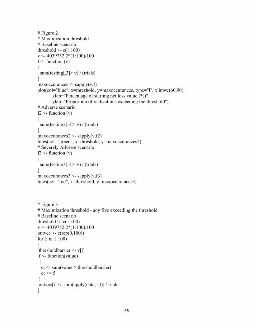
Appendix 3: Sample Analysis

In this section, the code used to produce some of the figures, including Figures 2,

3, 6, 7 and 11, is provided. For brevity, some of the code used in the What If Analysis is

omitted, but can easily be obtained by making modifications to the code that is provided.

49

# Figure 2 # Maximization threshold # Baseline scenario threshold <- c(1:100) v <- 4039752.2*(1:100)/100 f <- function (v) { sum(testing[,3]> v) / (trials) } maxoccurances <- sapply(v,f) plot(col="blue", x=threshold, y=maxoccurances, type="l", xlim=c(60,90), xlab="Percentage of starting net loss value (%)", ylab="Proportion of realizations exceeding the threshold") # Adverse scenario f2 <- function (v) { sum(testing2[,3]> v) / (trials) } maxoccurances2 <- sapply(v,f2) lines(col="green", x=threshold, y=maxoccurances2) # Severely Adverse scenario f3 <- function (v) { sum(testing3[,3]> v) / (trials) } maxoccurances3 <- sapply(v,f3) lines(col="red", x=threshold, y=maxoccurances3) # Figure 3 # Maximization threshold - any five exceeding the threshold # Baseline scenario threshold <- c(1:100) v <- 4039752.2*(1:100)/100 outvec <- c(rep(0,100)) for (i in 1:100) { thresholdbarrier <- v[i] f <- function(value) { ct <- sum(value > thresholdbarrier) ct >= 5 } outvec[i] <- sum(apply(data,1,f)) / trials }

50

plot(col="blue", x=threshold, y=outvec, type="l", xlim=c(10,75), xlab="Percentage of starting net loss value (%)", ylab="Proportion of realizations exceeding the threshold") # Adverse scenario outvec2 <- c(rep(0,100)) for (i in 1:100) { thresholdbarrier <- v[i] f2 <- function(value) { ct <- sum(value > thresholdbarrier) ct >= 5 } outvec2[i] <- sum(apply(data2,1,f2)) / trials } lines(col="green", x=threshold, y=outvec2) # Severely Adverse scenario outvec3 <- c(rep(0,100)) for (i in 1:100) { thresholdbarrier <- v[i] f3 <- function(value) { ct <- sum(value > thresholdbarrier) ct >= 5 } outvec3[i] <- sum(apply(data3,1,f3)) / trials } lines(col="red", x=threshold, y=outvec3) # Figure 6 # Maximization threshold - first ten exceeding the threshold # Baseline scenario threshold <- c(1:100) v <- 4039752.2*(1:100)/100 f <- function (v) { sum((data[,2]> v) & (data[,3] > v) & (data[,4]> v) & (data[,5] > v) & (data[,6]> v) & (data[,7]> v) & (data[,8] > v) & (data[,9]> v) & (data[,10] > v) & (data[,11]> v)) / (trials) } maxoccurances <- sapply(v,f) plot(col="blue", x=threshold, y=maxoccurances, type="l", xlim=c(0,70), xlab="Percentage of starting value (%)",

51

ylab="Proportion of realizations exceeding the threshold") # Adverse scenario f2 <- function (v) { sum((data2[,2]> v) & (data2[,3] > v) & (data2[,4]> v) & (data2[,5] > v) & (data2[,6]> v) & (data2[,7]> v) & (data2[,8] > v) & (data2[,9]> v) & (data2[,10] > v) & (data2[,11]> v)) / (trials) } maxoccurances2 <- sapply(v,f2) lines(col="green", x=threshold, y=maxoccurances2) # Severely Adverse scenario f3 <- function (v) { sum((data3[,2]> v) & (data3[,3] > v) & (data3[,4]> v) & (data3[,5] > v) & (data3[,6]> v) & (data3[,7]> v) & (data3[,8] > v) & (data3[,9]> v) & (data3[,10] > v) & (data3[,11]> v)) / (trials) } maxoccurances3 <- sapply(v,f3) lines(col="red", x=threshold, y=maxoccurances3) # Figure 7 # First Quartile # Baseline scenario Quarter = c(1, 2, 3, 4, 5, 6, 7, 8, 9, 10, 11, 12, 13, 14, 15) apply(data, 2, quantile,.25) TwentyfifthPercentile <- c(2823417.87, 2068815.22, 1564829.41, 1234486.55, 1001875.97, 856735.49, 745969.04, 669664.83, 613680.57, 580760.81, 575391.27, 584599.51, 587573.51, 595768.27, 602933.16) plot(col="blue", x = Quarter, y = TwentyfifthPercentile, type="l", xlab="Quarter", ylab="25th Percentile of Net Loss") # Adverse scenario apply(data2, 2, quantile,.25) TwentyfifthPercentile2 <- c(2907191.50, 2274786.19, 1938761.29, 1705450.74, 1593400.03, 1526540.88, 1471302.23, 1414210.67, 1370268.64, 1307796.72, 1263760.79, 1222805.79, 1188417.48, 1156754.62, 1125066.42) lines(col="green", x = Quarter, y = TwentyfifthPercentile2) # Severely Adverse scenario apply(data3, 2, quantile,.25) TwentyfifthPercentile3 <- c(2955091.12, 2396380.19, 2170275.71, 2105009.06, 2171486.95, 2202220.04, 2188584.76, 2115629.29, 2063693.02, 1964874.98, 1896808.42, 1817234.87, 1751594.89, 1682041.87, 1627902.58) lines(col="red", x = Quarter, y = TwentyfifthPercentile3)

52

#Figure 11: The cumulative net loss values for the Baseline scenario for every trial Percent <- 1:23000000 CumulativeNetLoss <- data.frame(CumulativeNetLoss=NA) for (i in 1:(trials)) { CumulativeNetLoss[i,1] <- sum(data[i,2], data[i,3], data[i,4], data[i,5], data[i,6], data[i,7], data[i,8], data[i,9], data[i,10], data[i,11], data[i,12], data[i,13], data[i,14], data[i,15], data[i,16]) } CumulativeNetLoss <- t(CumulativeNetLoss) par(mfrow = c(1,1)) hist(CumulativeNetLoss, col="blue", breaks=20, freq = FALSE, xlim=c(10000000,40000000), xlab="Cumulative Net Loss", ylab="Frequency of Cumulative Net Loss")

53

Bibliography

"2016 Supervisory Scenarios for Annual Stress Tests Required under the Dodd-Frank Act Stress Testing Rules and the Capital Plan Rule." DFAST. Board of Governors of the Federal Reserve System, 2016. Web. 7 Apr. 2017. <http://www.federalreserve.gov/newsevents/press/bcreg/bcreg20160128a2.pdf>. "2017 Supervisory Scenarios for Annual Stress Tests Required under the Dodd-Frank Act Stress Testing Rules and the Capital Plan Rule." DFAST. Board of Governors of the Federal Reserve System, 2017. Web. 7 Apr. 2017. <https://www.federalreserve.gov/newsevents/pressreleases/files/bcreg20170203a5.pdf>. Campbell, Harvey R. "Definition of "Pre-Provision Net Revenue"." NASDAQ. N.p., 2011. Web. 07 Apr. 2017. <http://www.nasdaq.com/investing/glossary/p/pre-provision-net-revenue>. "Effective Federal Funds Rate." FRED. N.p., 03 Apr. 2017. Web. 07 Apr. 2017. <https://fred.stlouisfed.org/series/FEDFUNDS>. "FRB: Supervisory Scenarios, Dodd-Frank Act Stress Test 2016: Supervisory Stress Test Methodology and Results June-2016." FRB: Supervisory Scenarios, Dodd-Frank Act Stress Test 2016: Supervisory Stress Test Methodology and Results June-2016. N.p., 9 Aug. 2016. Web. 07 Apr. 2017. <https://www.federalreserve.gov/bankinforeg/stress-tests/2016-Supervisory-Scenarios.htm>. "Gross National Product." FRED. N.p., 30 Mar. 2017. Web. 07 Apr. 2017. <https://fred.stlouisfed.org/series/GNP>. "Uniform Bank Performance Report Interactive User's Guide." FFIEC Central Data Repository's Public Data Distribution. Federal Financial Institutions Examination Council, n.d. Web. 07 Apr. 2017. <https://cdr.ffiec.gov/Public/Reports/InteractiveUserGuide.aspx?LineID=609957&Rssd=480228&PageTitle=Balance%2BSheet%2B%24&Concept=UBPRE119%2CUBPRE141%2CUBPRE027&ReportDate=3%2F31%2F2016>. "Uniform Bank Performance Report Interactive User's Guide." FFIEC Central Data Repository's Public Data Distribution. Federal Financial Institutions Examination Council, n.d. Web. 07 Apr. 2017. <https://cdr.ffiec.gov/Public/Reports/InteractiveUserGuide.aspx?LineID=609712&Rssd=480228&PageTitle=Summary%2BRatios&Concept=UBPRE019&ReportDate=3%2F31%2F2016>.

54

"View -- Uniform Bank Performance Report." FFIEC Central Data Repository's Public Data Distribution. Federal Financial Institutions Examination Council, n.d. Web. 07 Apr. 2017. <https://cdr.ffiec.gov/public/Reports/UbprReport.aspx?rptCycleIds=87%2C82%2C86%2C81%2C76&rptid=283&idrssd=480228&peerGroupType=&supplemental=>. "World's Largest Banks 2017." Banks around the World. N.p., 2017. Web. 07 Apr. 2017. <http://www.relbanks.com/worlds-top-banks/market-cap>.

55

Curriculum Vitae

Hannah Folz was born in London, UK, and grew up in Munich, Germany. She

attended Munich International School, and graduated with the International Baccalaureate

in May 2013. At Johns Hopkins University, she will complete a double-major in Applied

Mathematics and Statistics, and English, in addition to earning her Masters Degree in

Applied Mathematics and Statistics in May 2017. Hannah also enjoyed serving as a

mentor through the Office of Multicultural Affairs, being a Course Assistant at the Center

for Leadership Education; and interning at Deutsche Bank AG and Audi AG in Germany.

She looks forward to working in Risk Consulting in the Financial Services Industry at

PricewaterhouseCoopers next fall.