a modern survey and holocene record of … · a modern survey and holocene record of lake water and...
TRANSCRIPT
A MODERN SURVEY AND HOLOCENE RECORD OF LAKE WATER AND
DIATOM ISOTOPES FROM SOUTH ALASKA
By Caleb J. Schiff
A Thesis
Submitted in Partial Fulfillment
of the Requirements for the Degree of
Master of Science
in Geology
Northern Arizona University
December 2007
Approved:
Darrell Kaufman, Ph.D., Chair
R. Scott Anderson, Ph.D.
Mary Reid, Ph.D.
Al Werner, Ph.D.

2
ABSTRACT
A MODERN SURVEY AND HOLOCENE RECORD OF LAKE WATER AND
DIATOM ISOTOPES FROM SOUTH ALASKA
CALEB SCHIFF
Oxygen isotopes of diatoms (!18Odiatom) record the isotopic composition of lake water
(!W) in lakes of maritime south Alaska and provide insights into past changes in
atmospheric circulation. Lake water and sediment were collected along an
elevational transect in south Alaska and analyzed for paleoclimate studies. !W and
climate data show a strong gradient from maritime to interior sites. In general, !W
from coastal lakes reflect the isotope composition of local precipitation (!P) and
define the local meteoric water line (LMWL), which is parallel to the global
meteoric water line. !W from interior lakes, however, are influenced by evaporation
and exhibit a lower slope (6 versus 8). !18Odiatom from modern sediments show a
strong correlation with !W (r = 0.99) and local mean annual air temperature (r =
0.94). The modern spatial relationships cannot be explained by temperature-
dependent fractionation effects alone, nor by physiographic characteristics of the
lakes (e.g., lake and watershed area), so cannot be used for quantitative
paleotemperature reconstructions. These analyses reaffirm the complexity of North
Pacific !P and the secondary role of temperature on !W values in the region. The
paucity of !P data from south Alaska further hampers paleotemperature

3
reconstructions. Changing wintertime moisture source is the most probable control
on regional !P, which is strongly linked to the intensity and position of the Aleutian
Low (AL).
Sediment cores were recovered from Mica Lake (60.96° N, 148.15° W; 100
meters above sea level), an evaporative-insensitive lake in the western Prince
William Sound. The lake sediment contains massive gyttja, sand-rich avalanche
deposits, and six tephra deposits. Thirteen calibrated ages on terrestrial and
macrofossil samples were used to construct an age-depth model for core MC-2 and
suggests that the core spans the last 9910 yr. The average sedimentation rate from
the age model is 0.30 mm/yr and the average uncertainty based on the 95%
confidence interval is ± 112 yr. Half-cm-thick samples, representing ~15 yr of
sedimentation, were sampled at different intervals from core MC-2. Contiguous
magnetic susceptibility measurements helped identify tephra deposits. Percent
organic matter (OM) and biogenic silica (BSi) record lake productivity. OM and BSi
have a first-order increase between 9.6 ka and 2.5 ka, then descreases towards 0.1 ka
and covary (r = 0.52).
Diatoms from 46, 0.5-cm-thick samples were isolated and analyzed for their
oxygen isotope ratios. The analyses employed a newly designed, stepwise
fluorination technique, which uses a CO2 laser-ablation system, coupled to a mass
spectrometer. !18Odiatom values range between 25.2 and 29.8‰ and have a
reproducibility of 0.2‰. !18Odiatom values are relatively uniform between 9.6 and 2.5
ka, but exhibit a four-fold increase in variability since 2.5 ka. The 20th century
shows a 4.6‰ increase of !18Odiatom. Late Holocene excursions to lower !18Odiatom

4
values suggest a more western or southwestern moisture source (Bering Sea)
delivered by zonal flow, while higher !18Odiatom values reflect more southern moisture
(Gulf of Alaska), delivered by meridional flow. Zonal flow likely corresponds to
weaker AL because the south-to-north storm track is less prominent, allowing
moisture from the west to reach south Alaska. Comparisons with regional !P
records support the moisture-source hypothesis and also document late Holocene
atmospheric instability.
This study is the first detailed investigation of !W from south Alaska. The
results provide a more complete understanding !W in south Alaska to be applied to
future paleoclimate studies from the region.

5
ACKNOWLEDGEMENTS
While intelligence and stubbornness has often helped me reach many
achievements in my life, completing this thesis required perpetual motivation. I
thank my advisor, Darrell Kaufman, for continued encouragement during the past
two years. Darrell is the definition of a great advisor: his attention to detail, rapid
turnover of drafts and emails, and his ability to sense his students extent of “burn-
out” helped me immensely, especially during this last semester. Completing this
thesis would not have been possible without his dedication to me and our research.
I thank my field assistants, Nick McKay, Tom Daigle, Chris Kassel, Eric
Helfrich, and Peggy Foletta for their hard work in often less-than ideal south Alaska
conditions. Our time spent playing Set-back and sharing glasses of “Killer-Juice”
after long days at Mica Lake will not be forgotten. Kristi Wallace provided
invaluable assistance in Anchorage and her hospitality and excellent food recharged
the field crew for continued field work. Kristi also advanced my understanding of
local tephra records and provided important geochemical data of tephra from Mica
Lake.
I thank Andrew Henderson for teaching me the finer points of diatom
isolation. Mastering the sensitive procedure was a necessity for success of this
thesis.
I thank Justin Dodd for his work towards refining the diatom analyses using
the laser-ablation mass spectrometer. It was exciting to develop the new
methodology that has advanced this research.

6
I thank Rick Doucett for his extra effort towards analyzing water isotopes
from my south Alaska collections.
I thank Ryan Vachon who guided and advised me through my early
undergraduate years at the University of Colorado. Ryan inspired and helped me to
pursue science while living life to its fullest, which is a balance I often struggle to
find. I also (jokingly) blame Ryan for sparking my interest in studying the stable
isotopes of precipitation, which can leave anyone feeling perplexed, frustrated, and
ready for a beer at the end of the day!
I thank my family and friends for being patient during the last two years.
Although I know they enjoy hearing stories and viewing pictures of research in
Alaska, my commitment to research requires me to spend less time with loved ones
and I am grateful for their understanding.
During the last five months, at home, work, and in the field, Heidi Roop has
added a new, exciting, and fulfilling dimension to my life. I am grateful for her
patience, warm meals, and attentive listening during stressful times. Warm Mochis
and afternoon coffee dates go a long way. I look forward to providing similar love
and support for her as she pursues her Master’s degree with Darrell.
I thank the Geological Society of America’s Limnology and Quaternary and
Geomorphology divisions for their support and awards. Recognition by these two
groups help me stay motivated and reaffirmed the quality of my work.
Funding for this research was provided by the National Science Foundation
(NSF: ARC-0455043), the US Geological Survey, the Geological Society of
America, and the Friday Lunch Clubbe.

7
TABLE OF CONTENTS
Page
Abstract.........................................................................................................................2
Acknowledgements .......................................................................................................5
List of Table................................................................................................................10
List of Figures .............................................................................................................11
Chapters
1. Introduction ..........................................................................................................12
2. Background ..........................................................................................................14
2.1. Stable isotopes of precipitation ............................................................................14
2.2. North Pacific climate variability and !P records .................................................16
2.3. Diatom oxygen isotopes as an archive of lake-water conditions ...........................18
3. Study site...............................................................................................................20
3.1. Mica Lake............................................................................................................20
3.2. Modern climate ...................................................................................................21
4. Methods ................................................................................................................22
4.1. Sediment core recovery, sampling, and geochronology ........................................22
4.2. Lake instrumentation ...........................................................................................23
4.3. Regional water and top-sediment sampling..........................................................23
4.4. Physical sediment analyses ..................................................................................24
4.5. Diatom isolation and analyses ............................................................................25
4.6. Water isotope analyses ........................................................................................27
5. Modern meteorological and water and diatom isotope analyses .........................27

8
5.1. Mica Lake meteorological correlations ...............................................................27
5.2. Regional water isotope data ................................................................................28
5.3. Prince William Sound lake and watershed characteristics and !W data...............29
5.4. Diatom oxygen isotopes from modern lake sediment ............................................31
6. Lake core results and interpretations ..................................................................34
6.1. Core chronology..................................................................................................34
6.1.1. 210Pb and 137Cs profiles .....................................................................................34
6.1.2. 14C age model ...................................................................................................35
6.2. Core description ..................................................................................................37
6.3. OM and BSi interpretation...................................................................................39
6.4. Diatom oxygen isotopes from Mica Lake .............................................................40
7. Controls on diatom oxygen-isotope variability at Mica Lake .............................40
7.1. Non-climatic controls ..........................................................................................40
7.2. Climatic controls .................................................................................................42
7.2.1. P/E balance ......................................................................................................43
7.2.2. Changes in !P at Mica Lake .............................................................................44
7.2.2.1. Seasonality of precipitation............................................................................45
7.2.2.2. Air temperature .............................................................................................46
7.2.2.3. Change in moisture source.............................................................................47
7.3. Links to the AL.....................................................................................................48
8. Comparisons with other North Pacific climate and paleo-isotope records .......49
8.1. Late Holocene climate variability ........................................................................49
8.2. Paleorecords of !P ..............................................................................................50
9
8.3. The Little Ice Age ................................................................................................53
8.4. The 20th century ..................................................................................................53
9. Conclusions ..........................................................................................................55
10. Works cited .........................................................................................................59
Appendices...............................................................................................................100

10
List of Tables
Page
1. Expression of the Aleutian Low in the eastern North Pacific ..................................73
2. Climate station site and summary data....................................................................74
3. Location, water depth, length, and notes for cores from Mica Lake ........................75
4. Characteristics and surface-water isotope values for surveyed lakes located within 210
km of Mica Lake ........................................................................................................76
5. Correlation matrix for PWS lake and watershed characteristics .............................77
6. Core top and trap diatom and lake-water isotope values..........................................78
7. 210Pb and 137Cs activity of gravity core MC-2-A and -C ..........................................79
8. Radiocarbon and calibrated ages from core MC-2 ..................................................80
9. List of tephra data from MC-2 ................................................................................81

11
List of Figures
Page
1. The wintertime expression of the AL in the North Pacific.......................................82
2. The North Pacific Index time series........................................................................83
3. Map of study area with location discussed in text ...................................................84
4. Mica Lake watershed and bathymetry.....................................................................85
5. Climate summaries of south Alaska........................................................................86
6. Diatom isolation flow chart ....................................................................................87
7. Backscattered electron images of isolated diatoms..................................................88
8. Mica Lake and Whittier daily air temperature relationship......................................89
9. Survey water sample data plotted in !18O and !D space .........................................90
10. Summary of south Alaska lake isotopes ...............................................................91
11. Lake and median watershed elevation and isotope comparisons............................92
12. Modern !18Odiatom and lake condition relationships ................................................93
13. 210Pb and 137Cs profiles..........................................................................................94
14. Spline-fit age model .............................................................................................95
15. Photo and MS profiles of typical MC-2 lithology .................................................96
16. MC-2 geochemical, physical, and chronological summary....................................97
17. Holocene Mica Lake !18Odiatom compared to North Pacific !P records ...................98
18. 20th century Mica Lake !18Odiatom and North Pacific Index......................................99

12
1. Introduction
Lake water isotopes (!W) integrate spatial and temporal changes in climate on a
variety of scales. For lakes with long water residence times, !W often varies with
the precipitation/evaporation balance (E/P), whereas !W in lakes with short
residence times more directly reflect the isotopic composition of precipitation (!P).
Empirical observations during the last ~50 years demonstrate the strong spatial and
temporal relationship between !P and environmental parameters (Dansgaard, 1964;
Rozanski et al., 1993). Perhaps most notable is the correlation between !P values
and latitude, with lower values towards the poles. However, departures from the
general poleward depletion are apparent from more detailed investigations of modern
and paleorecords of !P (e.g., Yurtsever and Gat, 1981; Boyle, 1997). Specifically,
large-scale vapor transport can change the origin and moisture pathway, which cause
different amounts of fractionation for a given site and latitude (Bowen and
Wilkinson, 2002). Because there are multiple controls on !P, unambiguous climate
interpretations are difficult without a more complete understanding of regional
effects on !P. Calibration between !P and climate can sometimes be obtained from
long-term site collections, but these data are sparse. Surveys of modern !W of a
region may be the best method to disentangle the spatial and temporal variability of
!P because lakes are spatially dense in some regions and provide ‘averaged’
conditions, which are most practical for paleoclimate interpretations.
Numerous components of lake sediments have been investigated for records
of !W, including: chironomid head capsules (e.g., Wooller et al., 2004; in prep.),
13
aquatic cellulose (e.g., Abbott et al., 2000; Sauer et al., 2001), and authigenic
carbonate (e.g., Abell and Hoelzmann, 2000; Hu et al., 2001; Anderson et al., 2005).
No one component is a panacea because of individual shortcomings. For example,
authigenic carbonate studies are limited to alkaline lakes and aquatic cellulose may
not be continuously preserved (e.g., Sauer et al., 2001). Also, non-climate controls
must be considered when using biogenic material because fractionation occurs
during formation, although laboratory and field studies provide good estimates of the
magnitude of fractionation effects during the transfer of isotopes from water to
sediment (e.g., Sauer et al., 2001; Moshen et al., 2005). Most recently, the oxygen
isotopes of lake diatoms (!18Odiatom) have emerged as an alternate proxy of paleo !W
(see review in Leng and Barker, 2006). Diatoms are ubiquitous in most lakes and
their silica structure ensures good preservation. Recent advances in diatom
separation techniques (Rings et al., 2004) and mass spectrometry (Dodd et al., in
press) have expanded the method to lakes with relatively low productivity. Studies
of !18Odiatom have been used as a record of temperature (e.g., Shemesh and Peteet,
1998; Hu and Shemesh, 2003), !P (e.g., Shemesh et al., 2001; Rosqvist et al., 2004),
and lake E/P (e.g., Lamb et al., 2005).
In this study, I investigate the oxygen isotope composition of water and
diatoms recovered from south Alaskan lakes and their respective watersheds. My
investigations reveal large spatial and temporal variability of !W and !18Odiatom. The
modern !W data span three climate regimes and the !18Odiatom temporal record from
one site extends to 9600 yr BP. The modern distribution of !W clearly demonstrates
that maritime !W reflects !P, whereas interior lakes are strongly affected by
14
evaporation. The current understanding of !P in the North Pacific region does not
allow a simple interpretation of the 9600 yr !18Odiatom record but multiple controls are
considered. I suggest that !P in south Alaska is strongly dictated by the moisture
source and therefore changing !W is driven by large-scale changes of North Pacific
atmospheric circulation. Specifically, the strength and position of the Aleutian Low
(AL) is suggested as the main control of !P in south Alaska.
2. Background
2.1. Stable isotopes of precipitation
A global survey of the isotopes of precipitation (!P), now operated by the
International Atomic Energy Agency’s Global Network for Isotopes in Precipitation
(IAEA-GNIP), began in the 1960’s in an effort to better understand the spatial and
temporal variability of !P and their link to climate. Empirical relationships between
!P and environmental parameters at collection stations (e.g., air temperature, amount
of precipitation, altitude, distance to coast) are well documented (Dansgaard, 1964;
Yurtsever and Gat, 1981; Rozanski et al., 1993; Araguás-Araguás et al., 2000). In
general, local relationships observed between !P and environmental parameters
described the amount of “rain-out” of moisture from its source due to preferential
loss of heavier isotopes (18O, D) (Dansgaard, 1964). Statistical analyses of the global
data set show that !P is most strongly correlated with average monthly temperature;
latitude, altitude, and amount of precipitation are of lesser importance (Yurtsever and
Gat, 1981). In addition to the amount of rain-out, !P is affected by moisture source

15
conditions (e.g., sea surface temperature, humidity, and windiness). The IAEA-
GNIP program has continued routine collections to add to this database, which
presently includes over 250,000 collections (Araguás-Araguás et al., 2000). Only
9% of collections are from sites above 60° latitude, however, and data from network
stations often have long gaps between collections. Thus, many areas of the globe
lack robust records of !P, hindering paleoclimate studies that use oxygen and
hydrogen isotopes in geologic archives. Interpolation and modeling of modern !P
and meteorological data has provided a more complete map of the spatial distribution
of !P (Bowen and Wilkinson, 2002). These maps highlight areas for future
monitoring and regions where large-scale vapor transport pathways prevent accurate
interpolation between IAEA-GNIP stations. Models are used to interpret records of
!P and the mechanisms that cause !P to vary in areas with little data (Bowen and
Wilkinson, 2002; Kavanaugh and Cuffey, 2003; Bowen and Ravenaugh, 2003;
Fisher et al., 2004).
Biogenic and abiotic minerals that precipitate in lake and marine water and
are preserved in deposits are archives of !W, but the influence of a wide range of
environmental variables prevents simple interpretations. By combining baseline
conditions (e.g., modern !P and !W distributions and meteorological data) with an
understanding of the formation effects on any particular archive, the relationship
between !P, !W, and a sediment record can be disentangled. Using records of !W as
a paleothermometer is common, although the influence of changes in location or
conditions of the moisture source are well documented in ice cores (e.g., Boyle et al.,

16
1997; Masson-Delmotte et al., 2005; Stenni et al., 2001), speleothems (e.g.,
Denniston et al., 1999), and lake sediment (e.g., Rosqvist et al., 2004).
2.2. North Pacific climate variability and !P records
Climate variability in the North Pacific is associated with large-scale, interannual
(e.g., El Niño-Southern Oscillation [ENSO]) and interdecadal (e.g., Pacific Decadal
Oscillation [PDO]) climate oscillations (Trenberth and Hurrell, 1994; Papineau,
2001; Moore et al., 2003). The PDO is often viewed as ENSO-like phenomena
associated with interdecadal climate variability because of their similar spatial
patterns (e.g., Mantua et al., 1997). In south Alaska, winter surface air temperature
and precipitation are largely determined by the strength and position of the Aleutian
Low (AL), a low-pressure system that steers wintertime storms inland to south
Alaska (Fig. 1a) (Rodionov et al., 2005). The AL has no observed influence on
summer conditions. The DJF North Pacific Index (NPI), calculated as the area-
weighted, sea-level pressure over the region 30°N-65°N, 160°E-140°W (Trenberth
and Hurrell, 1994), provides a measure of the intensity of the wintertime AL (Fig. 2).
Negative NPI is associated with a strong AL. The interdecadal variability of the AL
is clearly seen when a 15 yr moving average is calculated from the annual DJF NPI
(Fig. 2). Strong shifts of the NPI have occurred three times during the 20th century,
centered at 1925, 1947, and 1977.
Modern and paleoclimate records of the AL have provided an understanding
of its direct regional influence. Rodionov et al. (2005) reviewed the meteorological
expression of the 10 strongest and weakest AL years between 1951 and 2000 in the
17
North Pacific (Fig. 1a; Table 1). The AL is split into two centers during weak years,
one in the Gulf of Alaska and one east of Kamchatka. In the Gulf of Alaska, storms
come from the west and northwest during weak AL years and from the southwest
during strong AL years. The increased southerly flow into the Gulf of Alaska brings
warm, moist air inland to south Alaska, which is well recorded at climate stations in
south-central Alaska (Fig. 1b). Inverse (cold and dry) conditions occur farther west
in the Aleutian Islands during strong AL years. Farther north at Anchorage, recorded
precipitation does not show much increase but average temperatures are 5 °C warmer
during strong AL years (Fig. 1b).
The AL’s link to storm intensity in the North Pacific (Trenberth and Hurrell,
1994; Rupper et al., 2004), its decadal variability during the 20th century (Overland et
al., 1999), and its predicted intensification and northward shift under global warming
(Yin, 2005; Salathé, 2006) is motivation to reconstruct the AL beyond historical time
periods. South Alaska is located along the North Pacific storm track and is therefore
an ideal location to record variability of the AL. Terrestrial climate records from this
area are strongly influenced by the AL. The mass balance of glaciers (e.g., Hodge et
al., 1998), organic matter in lake sediments (e.g., McKay, 2007), increases in far-
traveled pollen (Spooner et al., 2003), the accumulation rate in ice cores from Mt.
Logan (Rupper et al., 2004), and the effective moisture in interior Yukon (Anderson
et al., 2005) have been interpreted as variability in the AL on decadal to millennial
time scales.
Paleo-!P records from the North Pacific region suggest that air temperature is
not the primary control on !P (e.g., Wake et al., 2002; Fisher et al., 2004; Anderson

18
et al., 2005). For example, !P data from Mt. Logan ice cores do not correlate
significantly with instrumental or paleotemperature records (Holdsworth et al., 1992;
Wake et al., 2002). Significant deviation between temperature-driven isotope
models and modern !P from IAEA-GNIP stations in the North Pacific suggest large-
scale vapor transport patterns may explain the weak relationship between air
temperature and !P (Bowen and Wilkinson, 2002). With only three IAEA-GNIP
sites in all of Alaska, and two in adjacent Yukon Territory (Fig. 3 inset), modern-
and paleo-spatial and seasonal variability of !P is largely unknown.
2.3. Diatom oxygen isotopes as an archive of lake-water conditions
Diatoms (Class Bacillariophyceae) are composed of an amorphous silica shell (SiO2 ·
nH2O) (i.e., “frustule”) and a thin, organic layer surrounding the frustule (Round et
al., 1990). The !18Odiatom value is dependent on the 1) temperature and 2) oxygen-
isotope composition (!18O) of the ambient water during diatom formation (Leng and
Barker, 2006). Where the lake water !18O is known, !18Odiatom can be used as a
palaeothermometer (Juillet-Leclerc and Labeyrie, 1987). Recent isotope analyses of
paired diatom and water samples suggest that the lake water !18O - !18Odiatom
fractionation effect is -0.2 ‰/°C (Labeyrie et al., 1984; Juillet-Leclerc and Labeyrie,
1987; Shemesh et al., 1992; Brandiss et al., 1998; Moschen et al., 2005). While
these studies have constrained the general temperature dependence of fractionation
between water and diatoms, quantifying temperature change from a sedimentary
sequence is difficult because estimating past changes of lake water !18O requires
many assumptions about regional climate, including moisture source, seasonality of

19
precipitation, and the E/P balance of the lake. Making assumptions about such
dynamic climate conditions during the past is difficult without supporting data.
Realistically, downcore changes in !18Odiatom reflect a combination of many climatic,
and potentially non-climatic, factors. Paleoclimate interpretations from
sedimentary !18Odiatom records should be drawn conservatively (Leng and Barker,
2006).
Diatom productivity is dependent on a host of climate and lake conditions
(e.g., temperature, nutrient availability, and lake mixing regime). In temperate lakes
maximum productivity, or “blooms,” follows spring or autumn lake mixing when
nutrients are most readily available. The seasonal timing of diatom formation is an
important consideration because the isotope signature is acquired during formation.
For example, in stratified lakes, surface water may become enriched in 18O through
the summer, and diatoms formed during early and late summer can have different
isotope values (e.g., Moschen et al., 2005).
Lake water residence time and the seasonal range of !P are also important.
Water in small, shallow lakes will be refreshed more rapidly than large, deep lakes.
Therefore, !18Odiatom will be more sensitive to seasonal !P in the former and mean
annual or long-term !P in the latter. However, if the seasonal range of !P of an area
is low, !18Odiatom would be insensitive to lake residence time or the timing of diatom
bloom.
20
3. Study site
3.1. Mica Lake
Mica Lake (informal name, 60.96° N, 148.15° W; 100 meters above sea level [m
a.s.l.]) is located on Culross Island in the western Prince William Sound (PWS) of
southern Alaska (Fig. 3). Whittier, AK, is approximately 29 km to the west-
northwest. Mica Lake was selected because the high precipitation rate in the PWS
likely limits the effect of evaporation on surface waters and the warm, maritime
setting likely increases lake productivity. The lake is topographically open with
numerous small stream inflows and one outflow, spilling water into a small pond
~30 m lower (Fig. 4), which discharges to the coast. The lake surface and drainage
areas are 0.8 and 4.0 km2, respectively. Lake surface water pH was 6.0 and 6.2, and
secchi-disk depth was 11.2 and 13.6 m, during June 2006 and August 2007,
respectively. Patchy snow cover in the watershed persisted well into July during
2006. During August 2007, snow was essentially absent from the catchment and
outflow discharge was much reduced, and two of the four inflows were dry.
Mica Lake fills a glacially over-deepened basin in a granite stock surrounded
by meta-sedimentary rocks (Beikman, 1980). The granite provides abundant mica,
which forms a distinctive component of the sediment. The east and southern slopes
descend steeply into the lake, forming cliffs at many locations. The western part of
the watershed is less steep, and the northern area is all within 30 m above lake level.
Slopes to the east and west sides of the watershed rise to summits 600 m a.s.l. within
0.75 and 1.25 km of the lake, respectively (Fig. 4). The steep slopes are prone to

21
snow avalanches and any weathered debris that accumulates on the impermeable
granite substrate is likely to flush into the lake during high precipitation events,
especially on the east slopes. The modern vegetation is Pacific coast forest (Ager,
1998). Sitka spruce (Picea sitchensis) arrived ~2.5 ka and mountain hemlock (Tsuga
mertensiana), which is most common in the Mica Lake watershed, arrived soon after
(Huesser, 1983).
3.2. Modern climate
To provide a regional climate summary, data from long-term climate stations in PWS
were used to calculate monthly averages (Table 2; Fig. 5). All data were obtained
from the Western Regional Climate Center of the Desert Research Institute
(http://www.wrcc.dri.edu/index.html; last accessed 24 September 2007). Only sites
with > 90% of data for the period 1980 – 2005 were used, which limited the number
of sites to five: Seward, Whittier, Cannery Creek, Valdez, and Cordova (Fig. 3).
PWS receives the highest precipitation rate during September (366 mm) and
December (347 mm). The warmest (13.2 °C) and coldest (-3.2 °C) months are July
and January, respectively (Fig. 5a). Using the same screening criteria, data from
three interior sites, Gulkana, Snowshoe Lake, and Tonsina were used for comparison
with the PWS sites. At the interior sites, precipitation is highest in July (44 mm) and
August (36 mm). The warmest (13.2 °C) and coldest (-20.1 °C) months are July and
January, respectively (Fig. 5b). The strong climate gradient is evidenced by reduced
precipitation and increased temperature range at the interior sites.

22
4. Methods
4.1. Sediment core recovery, sampling, and geochronology
In June 2006, three percussion cores (7.6 cm diameter) and companion gravity cores
(6.5 cm diameter) up to 3.1 and 0.3 m, respectively, were recovered from Mica Lake
from depths " 58 m (Table 3). Coring at site 2 (Fig. 4) was presumably halted by the
bedrock as evidenced by freshly broken granite fragments lodged in the bottom of
the percussion core. The percussion (MC-2) and gravity core (MC-2-C) from core
site 2, here after collectively referred to as “MC-2,” is the longest recovered
sediment sequence and is the focus of this study. One of the three gravity cores from
site 2 (core MC-2-A) was extruded and subsampled at contiguous 0.25 cm intervals
in the field. All cores and bagged samples were shipped to Northern Arizona
University (NAU). Cores were split, photographed, and stored at 4 °C. Sediment
characteristics and tephra horizons from a fresh surface were described and assigned
a Munsell soil color. For physical sediment and diatom analyses, the top 5 cm of
sediment were sampled contiguously at 0.5 cm intervals, which was expanded to 5
and 10 cm spacing down to 100 and 310 cm, respectively. Samples were spaced for
higher resolution upward to provide more detail, presumably, during the last two
centuries (0 to 5 cm, contiguous sampling) and the last 2000 years (10 to 100 cm, 5
cm sampling) with coarse-sampling for the remainder of the core (100 to 300 cm, 10
cm sampling).
For radiocarbon analyses, 0.5-cm-thick samples were collected at 20 cm
spacing, or where vegetation macrofossils were visible, sieved and dried under a

23
laminar-flow hood. AMS 14C analyses were completed at the Keck Carbon Cycle
AMS Facility, University of California, Irvine or the Lawrence Livermore National
Laboratory, Riverside, CA. Contiguous 0.5 cm samples were also collected from
MC-2-C for 210Pb and 137Cs gamma spectrometry analyses at the University of
Southern California.
4.2. Lake instrumentation
Sediment traps were deployed at core site 2 at 10 and 58 m below the lake surface in
June 2006 and collected and redeployed in August 2007. Water temperature loggers
along side the traps and an air temperature logger on the north side of the lake (Fig.
4) recorded local water and air temperature conditions at 2 hr intervals from June
2006 to August 2007.
4.3. Regional water and top-sediment sampling
Lakes selected for water and top-sediment sampling are within 210 km of Mica Lake
and range in elevation from 9 to 1160 m a.s.l. (Table 4; Fig. 3). The sampling
strategy included a regional elevational gradient encompassing lakes from three
climate regimes of southern Alaska: maritime, transition, and interior (Papineau,
2001). The three climate regimes are in close proximity to one another because the
Chugach Mountains, rising 4000 m and spanning about 500 km, act as an effective
moisture barrier, thereby causing strong temperature and precipitation gradients
across zones. In general, the maritime zone receives higher precipitation (2920
mm/yr) and has lower seasonal temperature ranges (from -3.2 to 13.2 °C) when

24
compared to the interior zone (270 mm/yr and from -20.1 to 13.2 °C) (Papineau,
2001) (Fig. 5). Both topographically open and closed (no surface outflow), as well
as glacially fed and non-glacial, lakes were sampled in nearly each climate zone
(Table 4).
Water samples from lake, stream, precipitation, glacier, and snowpack were
collected across south-central Alaska during the summers of 2006 and 2007 (Fig. 3).
Water samples were collected in 15 mL polyethelene bottles with little or no
headspace, and sealed with vinyl tape. Lake surface waters were collected from the
approximate center of the lake or from the littoral zone when logistical constraints
limited boat access. The bottles were kept frozen or cool whenever possible.
To investigate the modern spatial distribution of !18Odiatom, the top 0.5 to 1.0
cm of sediment from 12 lakes was collected using a gravity corer. Logistical
constraints (i.e., boat access) did not allow for top-sediment sampling at all lakes
sampled for water.
4.4. Physical sediment analyses
Each sampled 0.5 cm interval from MC-2 was measured for organic-matter content
(OM) by weight loss on ignition, and biogenic silica content (BSi) using a wet-
alkaline extraction adapted from Mortlock and Froelich (1989). Both OM and BSi
of lake sediment have been successfully used to study past changes in lake and
watershed productivity (e.g., Nesje and Dahl, 2001; Hu et al, 2003; Nesje et al.,
2004; McKay, 2007). The two physical sediment characteristics measure the amount
of preserved biogenic material. At Mica Lake, OM and BSi provided proxies of

25
environmental change to corroborate !18Odiatom changes. BSi also helped forecast the
success of the diatom isolation procedure (see below) because diatom isolation is
inherently dependent on diatom abundance.
Magnetic susceptibility (MS) was measured on split-core faces at contiguous
0.5 cm intervals using a Bartington MS2 meter with Surface Scanning Sensor MS2E.
MS primarily reflects the abundance of magnetic grains and was used to locate
tephra horizons and confirm bulk lithology changes because tephra and minerogenic
sediment contain magnetic grains, which are absent in OM and BSi.
4.5. Diatom isolation and analyses
Diatoms from 46, 0.5-cm-thick samples sampled at contiguous to 10-cm-spaced
intervals were isolated and analyzed for their oxygen-isotope composition. Pure
diatoms must be isolated because other lake sediments (e.g., tephra, mineral grains,
organic matter) contain oxygen that would be liberated during vaporization of the
sample for mass spectrometer analyses (Leng and Barker, 2006). A three-stage
protocol involving chemical digestion, wet sieving, and heavy-liquid separation (Fig.
6) was adapted from Morley et al. (2004). The isolation technique was optimized to
best separate diatom from the ambient sediment in core MC-2. Diatom extracts were
screened for purity using a high-powered microscope, and a scanning electron
microscope was used to further confirm the purity of selected intervals (Fig. 7). The
10 to 50 µm size fraction was found to be most pure because it removed clay and
coarse silt.

26
The silica tetrahedra of diatom frustules can be divided into two parts: an
outer, hydrous layer and a dense, inner layer. While oxygen in the inner layer is
isotopically homogenous, the outer layer freely exchanges with the ambient water
after formation (Juilliet, 1980). Therefore, the outer silica tetrahedra must be
removed prior to mass spectrometry analyses to obtain an isotope value
representative of lake water during formation. Numerous methods have been used to
remove the outer hydrous layer, including vacuum dehydration, isotope exchange,
and stepwise fluorination (see review in Leng and Barker, 2006). Most recently, a
stepwise fluorination technique was designed that uses a CO2 laser-ablation system,
coupled to a mass spectrometer (Dodd et al., in press). This study is the first to
employ the new method to analyze lacustrine diatoms. The new technique is rapid
and requires only 1.0-2.0 mg of pure diatoms, which is less than the 5 mg typically
used for stepwise fluorination techniques. !18Odiatom analyses were completed at the
University of New Mexico, Albuquerque, NM. One in-house quartz standard, Gee
Whiz (!18O = 12.5 ± 0.15‰), and an in-house diatomite standard, SR2-1B (!18O =
32.3 ± 0.2‰), were routinely run with each batch of 10-18 samples. Gee Whiz has
been calibrated to the international NBS quartz standard (!18O = 9.6‰). Duplicate
analyses of 10 randomly selected samples from the MC-2 sequence have an average
reproducibility of ± 0.2‰, which is the uncertainty assigned to diatom samples
analyzed over the course of this study. The results are presented as conventional
permil deviations from the V-SMOW standard.

27
4.6. Water isotope analyses
Hydrogen and oxygen isotope ratios of water samples were measured with a
Thermo-Finnigan Deltaplus XL gas isotope-ratio mass spectrometer interfaced to a
Thermo-Electron Gasbench II headspace equilibration device at the Colorado Plateau
Stable Isotope Laboratory (http://www.isotope.nau).! Analytical precision on internal
working standards was ± 1‰ for !D and ± 0.1‰ for !18O. Hydrogen and oxygen
isotope ratios are presented in permil deviations from the V-SMOW standard.
5. Modern meteorological and water and diatom isotope analyses
5.1. Mica Lake meteorological correlations
The air temperature logger at the north end of Mica Lake operated continuously from
3 July 2006 to 12 August 2007. These data show that the warmest (15.0 °C) and
coldest (-11.8 °C) days occurred on 8 August 2007 and 7 January 2007, respectively.
The average annual temperature (3 July 2006 to 2 July 2007) was 2.8 °C. Daily
temperature data from Whittier (Fig. 3) is strongly correlated (r = 0.97) with
temperature at Mica Lake (Fig. 8a). The seasonal relationships are strong as well;
during the summer, the relationship between Mica Lake and Whittier temperature is
non-linear with higher-amplitude temperature fluctuations at Whittier than at Mica
Lake. From the daily average temperate data, lapse rates (lapse rate between two
sites = # temperature ÷ # elevation) were calculated, and the daily temperature at the
median elevation of the Mica Lake watershed (364 m a.s.l.) was calculated. Median
watershed elevation is defined as the elevation halfway between the lake elevation

28
and the highest elevation within a watershed. These temperatures were then
combined with precipitation data from Whittier to estimate the number of days with
snowfall at the Mica Lake watershed (gray vertical bars, Fig. 8b). I assumed that,
when precipitation was recorded at Whittier, it extended to Mica Lake, which is
probably correct considering their proximity (29 km). These analyses show that days
with snowfall make up 70% of precipitation days at Mica Lake, and that snowfall
occurs between mid-September and early June, with peak precipitation during mid-
September to early November, early December to February, and early April to mid-
June.
5.2. Regional water isotope data
!W values in water collected from south Alaska during the 2006 and 2007 summers
range from -22.6 to -5.9‰, and -176.1 to -37.6‰ for !18O and !D, respectively (Fig.
9a). Data from each of the three climate zones define local water lines (Fig. 9b-c;
Fig. 10b). Broadly, !W values trend from heavy to light and back to heavy values
along the south-to-north moisture pathway (Fig. 10a). In PWS, !18O and !D define
the local meteoric water line (LMWL), which is parallel to the global meteoric water
line (GMWL) (Fig. 9b). In the transitional climate zone, !18O and !D are generally
lower and the data define a local evaporation line (LEL), which has a slope (~6) less
than the LMWL and GMWL (8) (Fig. 9c). The lower !W values reflect the cooler
temperatures at the higher sites sampled in this climatic zone and rain-out as
moisture is transported north over the Chugach Mountains (Fig. 10a). The reduced
slope is due to enrichment of surface water in !18O, relative to !D caused by

29
evaporation (Gat, 1981) and therefore departs from the GMWL. Similarly, water
from the interior sites is relatively heavy, with a slope (~6) parallel to the LEL (Fig.
9d). Heavy !18O and relatively light !D values at interior sites are due to
evaporation.
In surface waters, deuterium excess (d.e. = !D – 8!18O) decreases because
evaporation affects fractionation of hydrogen and oxygen differently (Dansgaard,
1964). For example, in the Canadian arctic and Baffin Island, evaporation during the
summer decreases surface water deuterium excess by as much as 15‰ (Gibson et al.,
1993; Sauer et al., 2001). The trend of decreasing deuterium excess from south to
north supports the idea that greater evaporation occurs farther inland (Fig. 10a). The
large difference in precipitation rates between PWS and interior sites and warmer
summers at interior sites (Fig. 5) are likely causes of the regional trends.
5.3. Prince William Sound lake and watershed characteristics and !W data
!W values of PWS lakes range from -134 to -93‰, and -17.5 to -12.9‰ for !D and
!18O, respectively, a relatively wide range for closely located sites that experience
relatively similar temperatures and precipitation rates. To better explain these data,
PWS !W values were compared with lake and watershed characteristics (Fig. 11;
Table 5). Lake and watershed area, lake elevation, median watershed elevation, and
the presence or absence of glaciers were tabulated from maps and aerial photos. The
lakes were divided into glacial and non-glacial groups because lake water in
glaciated catchments inherits meltwater derived from past precipitation during
summer melting. Most lake characteristics are covariant with one another, with

30
stronger covariance for glacial than non-glacial lakes (Table 5). The correlation
between !W and lake and watershed elevations are weaker for glacial than non-
glacial lakes, but the correlation between lake and watershed area is stronger for
glacial lakes.
The strongest correlations are between !W and elevation. Median watershed
is more strongly correlated than lake elevation (Table 5; Fig. 11). For non-glacial
lakes, the r-values for !W and median watershed elevation are -0.95 and -0.90 for
!18O and !D, respectively, and are highly significant (p < 0.0001 for !18O; p < 0.01
for !D). For glacial lakes, the correlations between !W and median watershed and
lake elevation are not as strong, and are not significant at the 90% confidence level
(Table 5). The stronger correlation with median watershed elevation than for lake
elevation is further evidence that PWS !W integrates and reflects !P.
The slope of the regression line for median lake elevation vs. lake water !18O
is -0.76‰/100 m for non-glacial lakes. This gradient is similar to the values reported
from snow samples collected between 1750 and 3350 m a.s.l. in the St. Elias
Mountains (-0.7 to -0.6‰/100 m) (Holdsworth et al., 1991). Vertical isotope models
and measurements from the coast to ~1000 m a.s.l. suggest a slope of -0.95‰/100 m
(Fig. 9a in Fisher et al., 2004).
At Mica Lake, surface, bottom, inflow, and outflow water (n = 15) have a
narrow range of !18O values (Fig. 10c). This observation, combined with similarity
to the GMWL, suggests that the lake is well mixed and evaporation does not greatly
alter its isotopic values.

31
5.4. Diatom oxygen isotopes from modern lake sediment
Pure diatoms were isolated from core tops of four lakes and trap sediment from one
lake in the study area (Table 6). Four of the lakes are located in the PWS and are
topographically open; one lake is located ~150 km north of PWS in the interior and
is topographically closed. The diatom abundance was too low in the top sediment
from most surveyed lakes to be used for !18O analysis. The !18Odiatom values from top
and trap sediment range from 22.7 to 29.8‰ (Fig. 12; Table 6). Compared with the
water from the same lake, the diatoms have an oxygen-isotope fractionation (# =
!18Odiatom - lake water !18O) between 38.5 and 42.8‰.
Modern lake conditions were compared with !18Odiatom. Mean annual and
summer (JJA) air temperatures were projected for each lake using a standard lapse
rate and temperatures from the nearest climate station with complete data for the last
15 yr (Table 6). A moist (6°C/km) and dry (10°C/km) adiabatic lapse rate was used
for the PWS and interior sites, respectively. The 15 yr climate window was selected
to coincide with the estimated age of the top 0.5 - 1.0 cm core-top sediment samples.
The summer temperature during the ice-free season (JJA) was selected because it
likely coincides with the timing of diatom productivity. The interior site was
excluded from correlations because it is a closed lake within a different climate
regime (low precipitation and large temperature range) than PWS sites (high
precipitation and limited temperature range) (Fig. 5). Under these conditions, the
P/E balance at the lake will likely influence the !W. This limited data must be
interpreted with caution, but provide a baseline on which to build.

32
On the basis of just four samples, !18Odiatom correlates most strongly with lake
water !18O (r = 0.99, p < 0.01), median watershed elevation (r = -0.97, p < 0.1), mean
air temperature (r = 0.94, p < 0.1), and summer air temperature (r = 0.87, p = 0.13)
(Fig. 12a - 12d) and are discussed below. The strong empirical relationship between
!18Odiatom and lake water !18O (Fig. 12a) suggests that lake water !18O is the dominant
control on !18Odiatom from these sites. Comparison of top sediment diatoms,
representing ~15 yr of sedimentation, and lake water, representing < 10 yr of
summer lake water, may be inaccurate because the mean age of diatoms is probably
older than lake water.
The relationship between !18Odiatom and median watershed elevation is
stronger when compared to lake elevation (Fig. 11e and 11f) and has a slope of -
1.73‰/100 m, which is nearly 2.5 times greater than that observed between lake
water !18$ and median watershed elevation (-0.76‰/100 m) (Fig. 11b). While
keeping in mind that the steep slope of !18Odiatom versus median watershed elevation
is calculated from only four samples, the increase in slope suggests an amplification
of !18Odiatom enrichment (depletion) at lower (higher) elevation during the last ~15 yr.
Analyses between lake and watershed characteristics and !18Odiatom provide no
interbasin mechanism to explain the greater increased slope (Table 5). If low and
high elevation sites receive moisture with different transport histories (e.g., distance
traveled and moisture source), the gradient could be explained by non-temperature
controls. For example, if high elevations receive on average more long-traveled
moisture (e.g., Bering Sea), greater rain-out would cause more depleted !18O of lake
water values relative to low elevation sites that receive only local moisture (e.g.,

33
Gulf of Alaska). Therefore, the increased slope of lake water !18O vs. !18Odiatom could
be explained if lake water !18O from my summer collections reflect a time when
different elevations received moisture from the same source and pathway, whereas,
!18Odiatom values reflect the integration of mixed moisture and pathway histories. This
hypothesis seems most logical because storm tracks are known to vary in the region
due to shifts in the position of the AL (Table 1; Fig. 1) and because lakes incorporate
multiple years of precipitation so lake water !18O likely reflects ‘average’ moisture
from different storm tracks.
The slopes of mean annual and summer air temperature vs. !18Odiatom (Fig. 12b
and 12c) are also steeper than would be predicted by simply combining the known
relationship between lake water !18O and !18Odiatom (-0.5 to -0.2 ‰/°Cwater) (e.g.,
Moshen et al., 2005) with the global range of temperature-dependent fractionation of
!P (0.2 to 0.9‰/°C) (e.g., Rozanski et al., 1993). Applying this range, the highest
value (0.7‰/°C) falls well short of the observed relationship between lake water
!18O and !18Odiatom. Again, this observation suggests additional feedbacks between
lake water !18O and !18Odiatom that are not presently understood, but are not likely due
to decreased temperature with increased elevation.
Uncertainties inherit to these analyses include: 1) the sparse dataset (n = 4),
2) the limited temperature range of the sample sites, 3) the site temperature
extrapolation, 4) the age of the modern diatom samples, which may encompass more
or less than the 15 yr estimate, 5) the differential timing of diatom bloom at each
lake, and 6) the presently unknown diagenetic effects. Lacking data to better
understand between-site variations in !18Odiatom, neither the relationships between
34
!18Odiatom and lake water !18O nor median watershed elevation can be used for
quantitative interpretations of climate from downcore variability of !18Odiatom.
6. Lake core results and interpretation
6.1. Core chronology
6.1.1. 210Pb and 137Cs profiles
Two gravity cores (MC-2-A and -C) were taken from the same site and measured for
210Pb and 137Cs activities (Table 7; Fig. 13). MC-2-A was extruded and sub-sampled
in the field at contiguous 0.25 cm intervals; MC-2-C was transported to NAU where
it was split and sampled at contiguous 0.50 cm intervals. The two cores show
similar, first-order trends, with 210Pb and 137Cs decreasing with depth, which supports
the general reproducibility of the analyses. In detail, however, the differences in the
two 210Pb profiles suggest a range of sedimentation rates. In core MC-2-A, the
relatively constant downcore 210Pb activity below 1.5 cm suggests a high
sedimentation rate. Conversely, the decrease of 210Pb from 2.75 to 3.25 cm in core
MC-2-C suggests a rapid decrease in sedimentation rate (Fig. 13a). The lithology of
this section of the core is uniform and there is no evidence of sedimentation rate
changes. Using a constant rate of supply (CRS) model for core MC-2-C suggests an
average sedimentation rate of 0.41 mm/yr, but a CRS model could not be constructed
for MC-2-A because the total excess 210Pb was not measured. The geochronological
significance of the 210Pb profile is presently unclear.

35
The 137Cs profiles are also difficult to interpret. In general, 137Cs should rise
from background values, reach a maximum, and then decrease to lower values near
the core top. The rise, crest, and descending trends correspond to the onset and peak
of nuclear weapons testing in the 1950’s and 60’s. The 1986 Chernobyl event has
been recognized in Northern Hemisphere glacier ice and lake sediments as a second,
younger peak in 137Cs profiles (e.g., Pinglot and Pourchet, 1995; Schiff et al., 2008).
The high values in the top 0.5 cm of MC-2-A suggest that the 1963 peak is captured
within this interval, whereas the initial rise at 2.75 cm and peak at 1.75 cm in MC-2-
C occurs deeper in the core (Fig. 13b). Therefore, the implied sedimentation rate
from MC-2-A is an order of magnitude less than from MC-2-C. Taken together the
210Pb and 137Cs data suggest sedimentation rates between 0.16 and 0.75 mm/yr, which
brackets the rate estimated by 14C ages (0.30 mm/yr; see below). However, with no
stratigraphic evidence to support the sedimentation rate changes implied by the 210Pb
profiles, and considering the contrasting 137Cs profiles, no accurate geochronological
information can be obtained from these data.
6.1.2. 14C age model
Sixteen 14C ages were calibrated to calendar years using the IntCal04 calibration
curve (Reimer et al., 2004) and CALIB (v 5.0.2; Stuiver and Reimer, 1993). I used
the median probability age output by CALIB as the single best estimate of the central
tendency of the calibrated age (Telford et al., 2004), and report all ages in reference
to cal yr AD 1950 (yr BP). Thirteen calibrated ages on terrestrial and aquatic
macrofossils (Table 8) and the age of the sediment surface (0 cm = -56 yr BP) were

36
combined to construct a depth-age model for core MC-2 (Fig. 14). Three ages were
not included in the age model because the terrestrial vegetation yielded ages older
than underlying ages, or they were from a sand-rich layer, interpreted to be an
avalanche deposit (see below). A spline fit was constructed using formulations from
Heegaard et al. (2005) and the statistical software R (http://cran.r-project.org; last
accessed 20 December 2007). The Heegaard procedure performs well for lake
sediment that contains abundant tephra layers (Schiff et al., 2008). The model takes
into account both the uncertainty in the calibrated ages as well as the uncertainty of
how well the age represents a particular core level. In addition to an age-depth
model, the procedure generates the 95% confidence intervals. The model requires
the selection of a k-value, which dictates how closely the spline approaches each
calibrated age. A high k-value will closely follow the ages, and the spline will have
more flexure whereas low k-values produce a rigid spline. A k-value of 7 was
selected for the MC-2 core because it is the lowest value that contains most of the 2
% ranges of the calibrated ages, and has relatively low model residuals, which is the
difference between the calibrated and estimated age of each dated levels. Using this
age model, the base of the core is extrapolated to 9910 yr BP and the average
sedimentation rate is 0.30 mm/yr. Therefore, each 0.5 cm sample represents ~15 yr
of sedimentation. The average age uncertainty based on the 95% confidence interval
is ± 112 yr. The basal age provides a minimum age of deglaciation at Mica Lake.

37
6.2. Core description
Based on MS, OM, BSi, and physical descriptions, sediment from MC-2 was divided
into three units: tephra, massive gyttja, and sand-rich layers (Fig. 15). Massive gyttja
units are brown (10YR, 2/2 or 3/4) with some color banding (10YR 4/2), whereas
sand-rich units include sand, pebbles, and abundant terrestrial vegetation
macrofossils and exhibit a wide spectrum of colors. Upper and lower contacts
between all units are sharp, although the uppermost sand-rich layer grades into the
overlying massive gyttja (Fig. 15). The MC-2 sequence contains 91% gyttja, 5%
sand-rich layers, and 4% tephra (Fig. 16). The gyttja contains relatively high OM
(19%) and BSi (5%), with low average MS (15 ± 19 SI, n = 565). Following the
sampling strategy outlined above, only one sand-rich layer was sampled for OM and
BSi and has lower OM (15%) and BSi (1.7%). Sand-rich layers have higher average
and more variable MS (120 ± 143 SI, n = 34). Tephra horizons exhibit the highest
average MS values (190 ± 155 SI, n = 23), and were not analyzed for OM and BSi.
OM and BSi range from 5 to 35% and 1.7 to 7%, respectively, and the two are
positively correlated (r = 0.52) (Fig. 16 graph inset). OM and BSi data are provided
in Appendix B-1. Sand-rich layers occur at three depths: 20.5 - 27.5, 185.5 - 196.0,
and 280.0 - 280.5 cm (tube depth) (Fig. 16). Coarse flecks of mica are visible on the
surface of gyttja and sand-rich layers.
The abundant macrofossils of terrestrial vegetation and coarse grains in sand-
rich layers suggest that these deposits are avalanche derived. Steep, sparsely
vegetated slopes (Fig. 4), with abundant snowfall and an ice-covered lake could
facilitate transport of such coarse material to core site 2. The presence of

38
minerogenic particles > 1 mm and macroscopic plant remains have been used as
proxies for snow avalanches. Lake sediment studies in Norway document snow-
avalanche deposits in lake basins with steep slopes (e.g., Seierstad et al., 2002; Nesje
et al., 2007). These studies corroborate the link between coarse-particle
sedimentation and terrestrial macrofossils with avalanche deposits.
Six visible tephra layers, ranging from 0.5 to 2.5 cm thick, are marked by
high MS values (Table 9; Fig. 16). All have sharp upper and lower contacts. The
uppermost tephra was used to splice together the percussion and gravity cores and
suggests that 6.5 cm was lost during percussion coring. The tephra and sand-rich
layers, interpreted as instantaneous deposits, were removed from the sediment
thickness to determine an adjusted depth below lake floor (blf) for core MC-2 (Fig.
16).
A hemlock needle directly below a tephra layer (2) at 35.25 cm (tube depth)
has a calibrated age of 1125 yr BP (Table 9; Fig. 14 inset). The tephra was initially
thought to correlate with the White River Ash (WRA), which has been dated to 1147
yr BP from 14C ages on trees buried by tephra in growth position near the summit
vent of Mt. Churchill volcano (Clague et al., 1995). However, preliminary
geochemical analyses suggest the tephras are not correlative (K. Wallace, personal
communication). The similar age of tephra 2 from Mica Lake and the WRA is an
important discovery because tephra deposits found around this time period are often
correlated to the WRA with little geochemical evidence.
From the k = 7 age model, a 0.5-cm-thick tephra layer (3) at 144.75 cm (tube
depth) has an interpolated age of 3950 yr BP, which is near the age of Hayes tephra
39
deposits found in south Alaska (e.g., Schiff et al., 2008). Visual inspection of the
sample shows characteristics (e.g., mineral assemblage) with known Hayes deposits
(K. Wallace, personal communication). However, without geochemical data,
identifying the deposit as Hayes tephra remains preliminary.
6.3. OM and BSi interpretation
Low sedimentation rates and inconclusive 210Pb and 137Cs ages from the upper part of
the Mica Lake cores prevent a detailed comparison between the proxy data and
meteorological data. Therefore, changes in OM and BSi provide only a qualitative
interpretation of environmental conditions at Mica Lake. Assuming that OM and
BSi are a proxy for productivity at Mica Lake, then productivity increased gradually
between 9.6 and 2.5 ka then decreased to 0.1 ka, although neither the long-term
increase nor decrease are monotonic (Fig. 16). The coefficient of variability is
greater for OM (32%) than for BSi (20%). The greater variability in OM suggests it
is sensitive or controlled by different environmental factors than BSi. Diatom
abundance is influenced by lake productivity related to water temperature, length of
ice-free season, rainfall, and nutrient availability (Anderson, 2000). The greater
variability may suggest that OM is influenced by the amount of terrestrial vegetation
transported to the lake from the adjacent, steep-walled watershed. Increased
terrestrial components of vegetation transported to the lake via episodic slope failure
and avalanches would likely cause greater variations in OM than BSi if diatom
abundance is more dependent on intralake factors. The preservation of at least three
avalanche deposits in MC-2 is evidence that lake sedimentation is influenced by such

40
watershed slope processes. Without further evidence (e.g., C:N ratios) this
explanation is only speculative.
6.4. Diatom oxygen isotopes from Mica Lake
Forty-six downcore !18Odiatom values from MC-2 range between 25.2 and 29.8‰ (Fig.
17a). Prior to 2.5 ka, the values range by only 2.2‰. At 2.5 ka, !18Odiatom exhibits a
strong shift to values that vary as much as 4.6‰. The youngest sample, which
represents the last ~15 yr contains the highest !18Odiatom value at 29.8‰. Within the
analytical precision of the laser-extraction technique (±0.2‰), only one other
sample, at 6.4 ka, is comparable (Fig. 17a).
7. Controls on diatom oxygen-isotope variability at Mica Lake
The large (4.6‰) variation in !18Odiatom from MC-2 cannot be due wholly to changes
in lake water temperature. Applying the lake water !18O - !18Odiatom fractionation of -
0.2 ‰/°C and assuming no change in !W suggests a lake-water-temperature range of
~23°C during the Holocene, which is untenable. Therefore, alternative controls must
be considered to explain the !18Odiatom variability.
7.1. Non-climatic controls
Diagenetic effects have been reported in studies that compare trap- and sedimentary-
diatom oxygen isotopes (Schmidt et al., 1997, 2001; Moschen et al., 2006). These
studies found a slow-acting maturation of diatoms that led to enrichment of 18Odiatom

41
after deposition. The authors attribute the enrichment to silica dissolution and
dehydroxylation, and suggest that !18Odiatom records with long-term trends of
enrichment with age should consider diagenetic effects as a leading explanation. No
studies investigating diagenetic effects have reported lower !18Odiatom values in older
sediment, however. Furthermore, backscattered electron images show no obvious
dissolution of modern (Fig. 7a; 0 cm) or mid-Holocene (Fig. 7b; 75 cm) diatom
frustules from MC-2. This observation, combined with the lack of a long-term trend
in the MC-2 record suggests that diagenetic effects are absent or undetectable at
Mica Lake.
Diatom habitat and taxonomic (vital) effects may influence !18Odiatom.
Because diatoms live in both benthic and planktonic settings, they experience
different temperatures throughout the year (Round et al., 1990). Benthic and
planktonic diatoms formed at the same time could have different isotope signatures,
particularly if the lake water !18O differs between habitats. At Mica Lake, however,
surface and bottom water during the June 2006 and August 2007 had nearly identical
!18O values (Fig. 10c), suggesting the lake is well mixed during the late spring and
summer.
Vital effects have yet to be documented for !18Odiatom and are expected to be
less than the analytical error of fluorination techniques (Leng and Barker, 2006). In
one of the most detailed !18Odiatom investigations to date, Moschen et al. (2005)
analyzed diatoms of three separate size ranges, each inferred to comprise different
diatom taxa. They found the same lake water !18O - !18Odiatom fractionation for each
size fraction, suggesting that diatoms are not influenced by a vital effect. From Mica

42
Lake, only the 10-50 µm size fraction was analyzed. While this size fraction was
selected primarily because of its purity, this narrow size range also likely limits the
number of taxa analyzed (Battarbee et al., 2001). In sum, a !18Odiatom vital effect is
likely nonexistent or undetectable in Mica Lake. An investigation of diatom flora
from MC-2 is in progress and will provide information to better address the potential
influence from habitat and vital effects by assessing the relative proportion of
benthic and planktonic taxon changes downcore.
7.2. Climatic controls
The inability of water temperature – diatom fractionation and non-climatic factors to
fully explain the large variability of Holocene !18Odiatom values suggests that the !W
at Mica Lake has varied over the last 9600 yr, and largely determined the
sedimentary !18Odiatom. This is further supported by two additional observations from
this study: 1) there is no apparent correlation between lake productivity (i.e., OM and
BSi) and !18Odiatom at Mica Lake (Fig. 16, inset graphs), even though productivity is
at least partly determined by temperature; and 2) the relationship between lake water
!18O and !18Odiatom is strong (Fig. 12a) whereas the temperature relationships are
inexplicable (Fig. 12b and 12c). The PWS slope of lake water !18O versus !18Odiatom
also encompasses the entire range of Holocene !18Odiatom values from MC-2. The two
primary controls on lake water !18O are the P/E balance and the !18O inflow to the
lake, both of which vary with climate.
43
7.2.1. P/E balance
The P/E balance and therefore lake hydrology strongly controls !W of lakes (Gat,
1981). !W data from the surveyed lakes exemplify this effect: interior lakes,
receiving low precipitation are topographically closed (Table 4), and evaporation at
these sites favors !D over !18O, which shift values from the GMWL (Fig. 9d) (Gat,
1981). In contrast, lakes in the PWS may receive an excess of 5 m of precipitation a
year (Fig. 5), and all but one of the surveyed lakes is topographically open (Jerome
Lake; Table 4). A small, topographically closed pond 200 m north of Mica Lake
(“MP” Fig. 4) was sampled in August 2007 and demonstrates the effect of summer
evaporation on surface water; the !18O is 4.3‰ higher than nearby Mica Lake (Fig.
10c). Surface and bottom water collected in June 2006 and August 2007 do suggest
a small progressive isotopic enrichment of surface water from summer evaporation.
!W values of bottom water are nearly identical between summers (-13.2 and -
13.4‰), whereas the surface water from August 2007 is 0.5‰ enriched relative to
June 2006. The enrichment is small when compared with the late Holocene 4.6‰
range of !18Odiatom at Mica Lake, and is irrelevant if diatom blooms always occur
during the late spring, prior to progressive evaporation through the summer months.
Furthermore, surface water inflow into Mica Lake collected during the summer is
indistinguishable from Mica Lake surface water (Fig. 10c).
Using a range of precipitation rates from 3 to 7 m/yr, which encompasses the
observed rate at Whittier during the last 25 yr (average = 5.5 m/yr), and assuming
that evapotranspiration is less than 0.5 m/yr, which is typical for south Alaska
44
(Newman and Branton, 1972), the lake water residence time is less than 5 yr at Mica
Lake. Lakes with such low residence time are relatively unaffected by evaporation.
Taken together, the high precipitation receipt, short water residence time,
nearly homogenous !W at Mica Lake (Fig. 10c), and overlap with the local meteoric
water line (Fig. 9), suggests that the modern !W is not strongly affected by
evaporation and instead is controlled largely by !P. This conclusion is further
supported by the long-term !18Odiatom record from Mica Lake. When strongly
influenced by evaporative effects, !W is typically variable and elevated, whereas the
opposite is true of wet periods (Leng and Marshall, 2004). At first glance, therefore,
the increased late Holocene variability in !18Odiatom at Mica Lake (2.5 ka to modern;
Fig. 17a) could reflect increased evaporation. On the other hand, the shift to lower
!18Odiatom values following 2.5 ka and the coincidence with the increased variability is
inconsistent with the hypothesis of increased evaporation.
7.2.2. Changes in !P at Mica Lake
Outside of the tropics, where the ‘amount effect’ is dominant, !P is determined by
local air temperature, but can also be influenced by changes in seasonality of
precipitation and changes in moisture source (Araguás-Araguás et al., 2000).
Realistically, each factor affects !P to some degree, and are discussed individually to
determine which controls are most influential.

45
7.2.2.1. Seasonality of precipitation
As previously discussed, ~70% of precipitation received at the Mica Lake watershed
is snow that falls between mid-September and early June (Fig. 8). Therefore, !P
(and !W) at Mica Lake is likely weighted towards winter precipitation. Seasonal
differences in !P could affect !W if the seasonality of precipitation has varied. The
relatively sparse IAEA-GNIP data available for the North Pacific region (Fig. 3
inset) provide some insight into the seasonal range of !P in south Alaska. The
maritime climate at the Adak IAEA-GNIP station, located 2000 km to the west is
most similar to Mica Lake. Between 1945 and 1970, the warmest (10.8 °C) and
coldest (0.6 °C) months at Adak were July and February, respectively, whereas the
wettest (199 mm) and driest (78 mm) months were December and July, respectively
(Vose et al., 1992). These data are similar to the PWS, where the minimum and
maximum seasonal temperatures are within 3 °C of Adak temperatures and
maximum precipitation rates occur in late fall and minimum precipitation rates occur
in early summer (Fig. 5a). Other sites (Bethel, Barrow, Mayo, and Whitehorse) are
located in different climate regimes (Papineau, 2001) (Fig. 3 inset).
The Aleutian Islands are strongly influenced by the AL (Rodionov et al.,
2005), although its expression at Adak is inverse to the AL expression in PWS (Fig.
1b). Correlations between the NPI and Adak DJF air temperature (r = 0.49) and
precipitation (r = 0.52) are reverse to Whittier DJF air temperature (r = -0.67) and
precipitation (r = -0.49). All correlations are significant at the 99% confidence level.
IAEA-GNIP data collected between 1962 and 1973 record mean summer (JJA)
temperature at Adak that is 9 °C higher than winter (DJF) temperatures, whereas

46
mean !18O is 0.4‰ higher in summer compared to winter. The correlation between
monthly temperature and !18O in precipitation is weak (r = 0.26) and is not
significant at the 90% confidence level. The relatively small seasonal range in !18O,
despite the large temperature range and the weak correlation between the two,
suggests that factors other than temperature strongly influence !P at Adak. Applying
the 18O - air temperature fractionation from the IAEA-GNIP global dataset
(0.65‰/°C; Rozanski et al., 1993) to the 9°C seasonal temperature range implies a
range of 5.9‰ between summer and winter, which is an order of magnitude greater
than what is recorded. The ‘amount effect,’ on the other hand, is more strongly
correlated in the Adak dataset: monthly !18O is inversely related to the amount of
precipitation (r = -0.50, p < 0.1). If the Adak data are representative of conditions at
Mica Lake, higher !18Odiatom might represent decreased precipitation, but is likely
insensitive to changes in seasonality of precipitation. The climatic similarity
between Adak and PWS is not a substitute for !P from PWS. To further investigate
the amount effect in the North Pacific, a phenomena that is common at low latitudes,
year-long collections are needed.
7.2.2.2. Air temperature
The global relationship between !P and temperature (i.e., ‘Dansgaard effect’) ranges
between ~0.2 and 0.9‰/°C (Rozanski et al., 1993). Applying this slope to the range
in !18Odiatom at Mica Lake (~4.6‰) suggests a shift of 5 to 23 °C during the late
Holocene. The upper estimate is not plausible, whereas the lower estimate is similar
to the DJF temperature range observed between the ten strongest and weakest AL
47
years at climate stations in south Alaska (Fig. 1b). The paucity of IAEA-GNIP data
from the region prevents an accurate measure of the influence that air temperature
has on !P. These results point to the need for a more extensive collection of waters
from south Alaska, especially in the winter.
7.2.2.3. Change in moisture source
The increase in the range of !18Odiatom values between the mid-19th century to present
(4.6‰) from MC-2 may more reasonably be explained by changes in moisture
source. Specifically, moisture from the west and north Pacific delivered by zonal
(west-to-east) flow is longer-traveled and likely more depleted than moisture
delivered by meridional (south-to-north) flow, which for south Alaska is likely from
the Gulf of Alaska (Cayan and Peterson, 1989). Moisture from zonal flow crosses
southwest Alaska and is susceptible to rain-out as it passes over the land, whereas
moisture from meridional flow travels over the Gulf of Alaska and rain-out is
significantly less. Furthermore, the Bering Sea probably contributes more moisture
under zonal than meridional flow and is likely more depleted isotopically because of
generally colder Bering Sea winter temperatures compared to Gulf of Alaska
temperatures (Locarnini et al., 2006). All available IAEA-GNIP data from Bethel
(1962-1965) show that, during the winter (DJF) !18O of precipitation is about 6‰
lighter than at Adak, and that Bethel DJF air temperatures are about 14 °C cooler
than at Adak. The cooler temperature and lighter isotope values suggest that Bethel
is more influenced by the Bering Sea while Adak is more influenced by the Pacific.
Without more complete collections of precipitation from storm tracks originating

48
from the two moisture sources, I cannot provide a quantitative estimate of the change
in !P. Nevertheless, !P changes from shifting moisture source are generally greater
than from temperature changes over the same time period (e.g., Terranes and
McKenzie, 2001).
7.3. Links to the AL
I suggest that variability in !18Odiatom at Mica Lake is largely controlled by the
location of the moisture source during the winter, which is closely linked to the
strength and position of the AL. The location of storm tracks during the winter
months are known to vary between strong and weak AL years (Rodionov et al.,
2005). During strong AL years, most storms tracks that intersect south Alaska have
a south-to-north trajectory and the moisture contribution from the Gulf of Alaska is
likely large (Fig. 1a). Precipitation during strong AL years is likely enriched in 18O
because the moisture is short-traveled. During weak AL years, storm tracks are more
often divided into two loci and the south-to-north storm trajectory is less prominent
(Fig. 1a). The weaker meridional flow might allow zonal flow to deliver moisture
from a more western or southwestern, North Pacific source (e.g., Bering Sea) to
reach south Alaska. Because this moisture would have been: 1) farther traveled, 2)
crossed an extensive landmass (~ 700 km), and 3) sourced from cooler waters, it
would be relatively depleted in 18O. Furthermore, air temperature in south Alaska
during strong AL years is about 5 °C warmer than weak AL years (Fig. 1b), which
supports the hypothesis of greater meridional flow. As previously mentioned, the
increased temperature would likely cause increased !18O and the seasonal variability
49
of !18O at the coastal IAEA-GNIP site is low (0.4‰), so greater winter precipitation
during strong AL years would not greatly reduce the annual !18O average.
Using this interpretation, the Mica Lake !18Odiatom record suggests that the
moisture delivery to south Alaska has shifted between zonal and meridional flow
during the last 2.5 ka (Fig. 17a). Low !18Odiatom values reflect zonal flow. Before 2.5
ka, the record is relatively stable and has generally heavy !18Odiatom values, suggesting
mainly meridional flow. Meridional flow is likely associated with a strong and
eastward AL, which is supported by the tendency of storms to track south-to-north
during strong AL years (Rodionov et al., 2005).
8. Comparisons with other North Pacific climate and paleo-isotope records
8.1. Late Holocene climate variability
Paleoclimate records across the North Pacific from lake sediments (e.g., Hu et al.,
2001; Spooner et al., 2002; Cockburn and Lamoureux, 2007; McKay, 2007), glacier
advances (e.g., Wiles et al., 2001), and tree rings (e.g., Wilson et al., 2007) suggest
late Holocene climate variability. Most records point to some influence from the
variability of the AL, usually building on the relationship between changes during
the 20th century and proxy data (e.g., Anderson et al., 2005; McKay, 2007). For
example, in a summary of pollen records from northwest North America, Spooner et
al. (2003) showed that the occurrence of far-traveled pollen increased at multiple
sites across northwest British Columbia between ~3 ka to present; the likely
mechanism is thought to be a long-lasting phase of strong AL because warm air is

50
more frequently carried inland during strong AL years and positive correlations
between the AL and instrumental temperature records were found. Climate records
also link ENSO variability and other indicators of equatorial convective activity to
the strength of the AL (White and Walker, 1973; Giese and Carton, 1999; Moore et
al., 2003), and an increase of ENSO frequency throughout the Holocene suggests a
trend towards increased instability of the inter-tropical convergence zone (Moy et al.,
2002; Koutavas et al., 2006), influencing wintertime conditions in the North Pacific
(Desar et al., 2004). Accumulation rates at Mt. Logan between 1948 and 1987 are
correlated with warm-phases of ENSO, which correspond to increased south-to-north
storm trajectories in the North Pacific (Moore et al., 2003). Similar to these Pacific
paleoclimate records, the large variability of !18Odiatom at Mica Lake suggests
dynamic pattern of atmospheric circulation during the late Holocene.
8.2. Paleorecords of !P
Paleorecords of !P from the North Pacific region are few, but a connection to large-
scale atmospheric circulation is beginning to emerge. Oxygen isotope ratios of
authigenic carbonate (!18Oca) from Holocene sediment of Jellybean Lake, Yukon
Territory, Canada (Fig. 3 inset) range by ~2‰ (Fig. 17b), which is too large to be
explained by changing water temperatures (Anderson et al., 2005). Rather, !18Oca at
Jellybean is interpreted as a proxy for the intensity and position of the AL. During
times of weak AL, less rain-out occurs because zonal flow carries moisture parallel
to the coastal mountains to reach Jellybean Lake. During times of strong AL,
meridional flow brings moisture directly against and over the St. Elias Mountains,
51
causing greater distillation. Therefore, strong AL years are recorded as low !18Oca
values. At Marcella Lake, an evaporative-sensitive lake in Yukon Territory, Canada
(Fig. 3 inset), oxygen isotopes of endogenic carbonate record effective moisture
(Anderson et al., 2007). The data suggests drier conditions occur during times of
strong AL because meridional flow brings stronger leeward winds to the Yukon
Territory. Times of strong (meridional flow) and weak (zonal flow) AL can
successfully explain the variability at Jellybean, Marcella, and Mica Lakes.
Meridional (zonal) flow causes high (low) !18O values at Mica Lake but low (high)
!18O values at Jellybean Lake because the coastal setting of Mica Lake limits rain-
out under meridional flow, while the interior setting of Jellybean Lake enhances rain-
out. At Mica Lake, zonal flow is associated with Bering Sea moisture and rain-out
over southwest Alaska, which is acknowledged by Anderson et al. (2007), whereas at
Jellybean Lake, less rain-out occurs because direct flow against the St. Elias
Mountains subsides.
Oxygen isotope values from an ice core (!18Oice) from the Mt. Logan summit
(Fig. 3 inset) does not correlate with instrumental or paleo-temperature from the
region (Holdsworth et al., 1992), although annual precipitation totals correlate with
North Pacific climate indices (Moore et al., 2002). The !18Oice values from Eclipse
Icefield (Fig. 3 inset) is significantly correlated with northwestern North America
temperature, but the correlation only explains between 5 and 10% of the variability
(Wake et al., 2002). These results suggest site temperature is not the primary control
of !P in the North Pacific.

52
Using an isotope model simulation, Fisher et al. (2004) suggest that isotope
variability at Mt. Logan and Jellybean Lake can be explained by shifting moisture
source. More specifically, two atmospheric flow regimes are prescribed for the
model and provide a mechanism to explain changes in !P: under the mixed
(meridional) flow regime, the moisture source includes low latitudes, whereas the
zonal flow regime derives moisture strictly from the high latitudes of the North
Pacific. The model predicts vertically stratified differences of !P between each flow
regime. The difference between mixed and zonal regimes [!18O (zonal) – !18O
(mixed)] above 1 km altitude is positive, and negative below 1 km. High-elevation
sites receive relatively light !P under mixed flow while low-elevation sites receive
heavy !P. The site response under different flow regimes would be opposite at Mica
Lake (median catchment elevation = 364 m a.s.l.) compared to Jellybean Lake
(effective catchment elevation = 1650 m a.s.l.) and Mt. Logan (5340 m a.s.l.). The
suggestion that the altitudinal variability of !P in the North Pacific is best explained
by changes in moisture source is consistent with the most plausible control at Mica
Lake.
In general, the variability !18O values during early and mid-Holocene at Mica
and Jellybean Lakes is lower than during the late Holocene (Fig. 17a and b). Mt.
Logan !18Oice does not show a late Holocene change to more variable values (Fig.
17c). The inverse relationship between !18O values at Mica Lake versus Jellybean
Lake and Mt. Logan is not strongly evident and depends on the quality of the
geochronology. However, the shift to more variable and lower !18Odiatom values at
Mica Lake at 2.5 ka is coincident with generally increasing !18O values at both

53
Jellybean Lake and Mt. Logan, suggesting that moisture delivery shifted from zonal
to meridional flow to all sites.
8.3. The Little Ice Age
The most recent shift to lower !18Odiatom values at Mica Lake coincides with the Little
Ice Age (LIA), a time of global cooling (Grove, 2004). The LIA is well documented
in the North Pacific region, enabling a detailed assessment of pan-North Pacific
climate variability. Most south Alaska glaciers reached their Holocene maxima
during the LIA (Wiles et al., 2007), suggesting that either summer temperature
reached its minimum, or that winter precipitation was at its maximum, or both.
Studies of glacier equilibrium-line altitudes find that lower summer temperatures and
lower winter precipitation occurred during the LIA; the latter suggest a weaker AL
(Daigle, 2006; McKay, 2007). Tree-ring records suggest that January to September
temperatures in the Gulf of Alaska were reduced by about 1 ºC during the LIA
(Wilson et al., 2007). These proxy records compare well with the low Mica Lake
!18Odiatom values of 26.0 and 25.8‰ at 1820 and 1845 AD, respectively, which is
interpreted as a period of weak AL, when south Alaska received proportionately
more moisture from zonal flow.
8.4. The 20th century
Shifts of North Pacific climate are well documented during the 20th century, and
provide a contemporary example of reorganization in the North Pacific that directly
influenced south Alaska. The shift during the 1976-77 winter (Fig. 18) included a

54
deepening of the AL, pushing southward and strengthening storm tracks in the North
Pacific (Miller et al., 1994). The 1976-77 shift is coincident with higher winter mass
balance at Gulkana and Wolverine glaciers in south-central Alaska, but decreased
winter mass balance at Cascade Glacier in Washington state, highlighting its broad
impact on western North America (Hodge et al., 1998). Alaskan salmon production,
which is dependent on marine productivity (Francis et al., 1998), has fluctuated at
interdecadal timescales during the 20th century, coincident with North Pacific climate
indices (Mantua et al., 1997). Similar 20th century shifts of Pacific climate occurred
in 1925 and 1947 (Fig. 18), and define the PDO polarity reversals, which are
positively correlated with the strength of the AL (Mantua et al., 1997). AL
variability during the 20th century provides a contemporary example of its impact on
storm-track trajectories intersecting south Alaska and its connection to other North
Pacific climate indices.
During the 20th century, !18Odiatom values at Mica Lake show a monotonic
increase (Fig 18). The top four contiguous MC-2 samples fall within the 20th century
and the next youngest sample (1880 AD) is used to plot the trend from the 19th to
20th. Each sample represents about 15 yr of sedimentation (not accounting for any
bioturbation), which is greater than the lake water residence time (< 5 yr).
Therefore, each !18Odiatom value integrates multiple seasons of diatom blooms. The
general increasing trend in !18Odiatom values contrasts with the 20th century winter
NPI, which shows the multidecadal variability of the AL (Fig. 18). However, both
time series have a first-order increasing trend over the 20th century. Sample
resolution and bioturbation at Mica Lake smooth the influence of multidecadal
55
climate variability, and results in a centennial-scale record of changing !P, so the
monotonic increase in !18Odiatom in spite of AL variability is understandable.
Although the first-order trends further suggest the link between the AL and !18Odiatom
values at Mica Lake, the small Mica Lake dataset limits a robust comparison.
9. Conclusions
The stable isotope ratios of water from south Alaska reveal a range of values across
climate regimes. !W from lakes in maritime settings closely reflect !P, whereas
water in interior lakes is strongly affected by evaporation. Water from lakes in the
transitional climate setting are also influenced by evaporation, but are isotopically
lighter due to colder temperatures at the higher-elevation sites sampled for this study.
Multiple lines of evidence support the evaporation insensitivity of maritime lakes
and the influence of evaporation at interior lakes, including 1) the !W values of
maritime lakes define a slope parallel to the GMWL (8), whereas !W values from
transitional and interior lakes have a lower slope (6), and 2) deuterium excess
decreases from maritime to interior sites implying greater evaporation of lake water
at interior sites. I found that !W at maritime lakes is more strongly correlated with
median watershed elevation than with lake elevation, indicating that these lakes are
good integrators of regional !P, not just !P over the lake site. Meteorological data
from the climate station at Whittier suggest that the majority of precipitation falls
during the winter months, when the atmospheric circulation is strongly influenced by
the AL. Therefore, if regional !P is influenced by the strength and position of the

56
AL, !W will likely change as well. The paucity of long-term precipitation
collections from south Alaska prevents a more robust test of this hypothesis,
however.
A smaller survey of lake sediment in lakes of maritime PWS exhibits a
!18Odiatom range larger than can be explained by temperature or the observed spatial
variability of !W. The offset between the expected mean diatom age (last ~15 yr)
and the age of the sampled water (few years) may partially explain the greater range
in !18Odiatom. Amplified (buffered) changes at high (low) elevation sites are also
required to explain the increased slope between !18Odiatom and elevation compared to
!W and elevation. Analyses of lake physiography reveal no reason for the greater
change in !18Odiatom relative to lake water !18O at the site. A steeper vertical gradient
of !P during the interval of time represented by !18Odiatom compared to the time
represented by lake water !18O would cause the larger range of !18Odiatom. Different
or mixed sources of moisture between high (isotopically light) and low (isotopically
heavy) sites is one mechanism that might explain the steep vertical !P gradient.
Both climatic and non-climatic factors influence !18Odiatom. Previous studies
have found enrichment of !18Odiatom due to dissolution during diagenesis. Little to no
dissolution of diatoms and no downcore trend towards enriched !18Odiatom suggests
that non-climatic factors are minimal. Low (0.4‰), intra-annual !18O of
precipitation recorded at Adak suggests the seasonality of precipitation is not an
important factor. I suggest that moisture source is the leading control, which seems
most plausible considering the link between the AL and wintertime precipitation in
south Alaska. Changes between meridional and zonal flow due to the changing

57
position and intensity of the AL would likely transport moisture from different
sources. Under zonal flow conditions, south Alaska would receive isotopically light
moisture because of greater rain-out and a colder source area (Bering Sea). South-
to-north moisture transport over the Gulf of Alaska under meridional flow conditions
would cause less rain-out and therefore be isotopically heavier.
I isolated diatoms from Holocene sediment from Mica Lake and measured
their oxygen isotope ratios. The large variability of !18Odiatom values (4.6‰) from the
9600 yr record can be best explained by shifting moisture source although,
realistically, !18Odiatom at Mica Lake integrates the effects of multiple controls.
During the early to mid-Holocene (~9.6 to 2.5 ka) !18Odiatom values at Mica Lake are
relatively high (28.6 ± 0.5 ‰) and stable. Since ~2.5 ka, brief, episodic decreases in
!18Odiatom suggests variable atmospheric circulation, which might be linked to large-
scale climate patterns in the tropical Pacific. The shift to decreasing lake
productivity inferred from the OM and BSi at Mica Lake is coincident with the shift
to more variable !18Odiatom, corroborating a change of environmental conditions
during the late Holocene. Low !18Odiatom values between ~1700-1900 AD coincide
with the LIA, a time of global cooling, and glacier expansion in south Alaska.
Similar times of lighter !18Odiatom occurred ~1.2 and 2.3 ka. Results from Mica Lake
suggest that the AL was weaker and more moisture was carried by zonal flow during
these times. During the 20th century, the NPI, a measure of the intensity of the AL,
and !18Odiatom, show first-order, increasing trends. The multidecadal variability of the
AL, however, is likely smoothed in the Mica Lake !18Odiatom record due to low sample
resolution.
58
!P paleorecords in the northern North Pacific show only weak correlations
with air temperature (e.g., Holdsworth et al., 1992; Wake et al., 2002) or have !18O
variations that are too great to be explained by changes in temperature (e.g.,
Anderson et al., 2005) and have been interpreted as “source meters” (Fisher et al.,
2004). The large variability of !18Odiatom from evaporative-insensitive Mica Lake also
suggests that moisture source has changed on centennial timescales. Viewed
collectively, the growing number of !P paleorecords from the North Pacific
emphasizes the variability of wintertime moisture delivery to northwestern North
America as a pervasive feature of the regional climate.
59
10. Works Cited
Abell, P.I., Hoelzmann, P., 2000. Holocene palaeoclimates in northwestern Sudan:
stable isotope studies on molluscs. Global and Planetary Change 26, 1-12.
Abbott, M.B., Wolfe, B.B., Aravena, R., Wolfe, W.P., Seltzer, G.O., 2000.
Holocene hydrological reconstructions from stable isotopes and
paleolimnology, Cordillera Real, Bolivia. Quaternary Science Reviews 19,
1801-1820.
Ager, T.A., 1998. Postglacial vegetation history of the Kachemak Bay Area, Cook
Inlet, south-central Alaska. In: Kelley, K.D., Gough, L.P. (Eds.), Geologic
Studies in Alaska by the US Geological Survey, 1998. US Geological
Survey Professional Paper 1615, pp. 147–165.
Anderson, J., 2000. Diatoms, temperature, and climate. European Journal of
Phycology 35, 307-314.
Anderson, L., Abbot, M.B., Finney, B.P., Burns, S., 2005. Regional atmospheric
circulation change in the North Pacific during the Holocene inferred from
lacustrine carbonate oxygen isotopes, Yukon Territory, Canada. Quaternary
Research 64, 21-35.
Anderson, L., Abbott, M.B., Finney, B.P., Burns, S.J., 2007. Late Holocene
moisture balance variability in the southwest Yukon Territory, Canada.
Quaternary Science Reviews 26, 130-141.
60
Araguás-Araguás, L., Froehlich, K., Rozanski, K., 2000. Deuterium and oxygen-18
isotope composition of precipitation and atmospheric moisture. Hydrological
Processes 14, 1341-1355.
Battarbee, R.W., Carvahlo, L., Juggins, S. Diatoms. In: Tracking Environmental
Change Using Lake Sediments, Vol. 3: Terrestrial, Algal, and Siliceous
Indicators, W. Last, J. Smol (Dordrecht, The Netherlands, Klumer, 2001),
155-202.
Beikman, H.M.,1980. Geologic map of Alaska; U.S. Geological Survey Professional
Paper PP 0171, unpaged, 1 plate.
Bowen G.L., Ravenaugh, J., 2003. Interpolating the isotopic composition of modern
meteoric precipitation. Water Resources Research 39,
doi:10.1029/2003WR002086.
Bowen, G.J., Wilkinson, B., 2002. Spatial distribution of !18O in meteoric
precipitation. Geology 30, 315-318.
Boyle, A.E., 1997. Cool tropical temperatures shift the global !18O -T relationship:
An explanation for the ice core !18O – borehole thermometry conflict?
Geophysical Research Letters 24, 273-276.
Brandriss, M.E., O’Neil, J.R., Edlund, M.B., Stoermer, E.F., 1998. Oxygen isotope
fractionation between diatomaceous silica and water. Geochemica et
Cosmochimica Acta 62, 1119–1125.
Cayan, D.R., Peterson, D.H., 1989. The influence of the North Pacific atmospheric
circulation on streamflow in the west. Geophysical Monograph 55, 375-379.

61
Clague, J., Evans, S., Rampton, V., Woodsworth, G., 1995. Improved age estimates
for the White River and Bridge River tephras, western Canada. Canadian
Journal of Earth Sciences 32, 1172-1179.
Cockburn, J.M.H., Lamoureux, S.F., 2007. Century-scale variability in late-summer
rainfall events recorded over seven centuries in subannually laminated
lacustrine sediments, White Pass, British Columbia. Quaternary Research 67,
193-203.
Daigle, T., 2006. Late Holocene climate change at Goat Lake, Keni Mountains,
south-central Alaska. M.S. Thesis, Flagstaff, AZ, Northern Arizona
University, pp. 128.
Dansgaard, W., 1964. Stable isotopes in precipitation. Tellus 16, 436-468.
Denniston, R.F., González, L.A., Asmerom, Y., Baker, R.G., Reagan, M.K., Arthur
Bettis. E., 1999. Evidence of increased cool season moisture during the
middle Holocene. Geology 27, 815-818.
Desar, C., Phillips, A.S., Hurrell, J.W., 2004. Pacific interdecadal climate
variability: linkages between the tropics and the North Pacific during boreal
winter since 1900. Journal of Climate 17, 3109-3124.
Dodd, J.P, Sharp, Z.D., Fawcett, P.J., Schiff, C., Kaufman, D.S., 2007. A laser-
extraction technique for oxygen isotope analysis of diatom frustules. EOS
Transactions, American Geophysical Union, in press.
Fisher, D.A., Wake, C., Kreutz, K., Yalcin, K., Steig, R., Mayewski, P., Anderson,
L., Zheng, J., Rupper, S., Zdanowicz, C., Demuth, M., Waszkiewicz, M.,
Dahl-Jensen, D., Goto-Azuma, K., Bourgeois, J.B., Koerner, R.M., Sekerka,

62
J., Osterberg, E., Abbott, M.B., Finney, B.P., 2004. Stable isotope records
from Mount Logan, Eclipse ice cores and nearby Jellybean Lake. Water
cycle of the North Pacific over 2000 years and over five vertical kilometers:
sudden shifts and tropical connections. Géographie physique et Quaternaire
58, 9033-9048.
Francis, R.C., Hare, S.R., Hollowed, A.B., Wooster, W.S., 1998. Effects of
interdecadal climate variability on the oceanic ecosystems of the NE Pacific.
Fisheries Oceanography 7, 1-21.
Gat, J.R., 1981. Isotopic fractionation. In: Gat, J.R. and Gonfiantini, R., editors,
Stable isotope hydrology, IAEA Technical Report Series 210, Vienna:
International Atomic Energy Agency, 21–33.
Gibson, J.J., Edwards, T.W.D., Bursey, G.G., Prowse, T.D., 1993. Estimating
evaporation using stable isotopes: Quantitative results and sensitivity analysis
for two catchments in northern Canada. Nordic Hydrology 24, 79-94.
Grove, J., 2004. Little Ice Ages. Routledge, London, ed. 2nd, pp. 402.
Giese, B.S., Carton, J.A., 1999. Interannnual and decadal variability in the tropical
and midlatitude Pacific Ocean. Journal of Climate 12, 3402-3418.
Heegaard, E., Birks, H.J.B., Telford, R.J., 2005. Relationships between calibrated
ages and depth in stratigraphical sequences: an estimation procedure by
mixed-effect regression. The Holocene 15, 612-618.
Hodge, S.M., Trabant, D.C., Krimmel, R.M., Heinrichs, T.A., March, R.S.,
Josberger, E.G., 1998. Climate variations and changes in mass of three
glaciers in western North America. Journal of Climate 11, 2161-2179.

63
Holdsworth, G., Fogarasi, S., Krouse, H.R., 1991. Variation of the stable isotopes of
water with altitude in the Saint Elias Mountains of Canada. Journal of
Geophysical Research 96, 7483-7494.
Holdsworth, G., Krouse, H.R., Nosal, M., 1992. Ice core climate signals from
Mount Logan, Yukon A.D. 1700–1897. In: Bradley, R.S., Jones, P.D. (Eds.),
Climate Since A.D. 500. Routelidge, London, 483–516.
Hu, F.S., Ito, E., Brown, T.A., Curry, B.B., Engstrong, D.R., 2001. Pronounced
climatic variations in Alaska during the last two millennia. Proceedings of
the National Academy of Sciences 98, 10552-10556.
Hu., F.S., Shemesh, A., 2003. A biogenic-silica the last glacial-interglacial transition
in southwester Alaska. Quaternary Research 59, 379-385.
Hu, F.S., Kaufman, D.S, Yoneji, S., Nelson, D., Shemesh, A., Huang, Y., Tian, J.,
Bond, G., Clegg, B., Brown, T., 2003. Cyclic variation and solar forcing of
Holocene climate in the Alaskan subarctic. Science 301, 1890-1893.
Heusser, C.J., 1983. Holocene vegetation history of the Prince William Sound
region, south-central Alaska. Quaternary Research 19, 337–355.
Juillet, A., 1980. Structure de la silice biogénique: nouvelles données apportees par
l’analyse isotopique de l’oxygène. CR Academy of Science 290, 1237–
1239.
Juillet-Leclerc, A., Labetrie, L., 1987. Temperature dependence of the oxygen
isotopic fractionation between diatom silica and water. Earth and Planetary
Science Letters 84, 69-74.

64
Kavanaugh, J.L., Cuffey, K.M., 2003. Space and time variation of !18O and !D of
Antarctic precipitation revisited. Global Biogeochemical Cycles 17,
doi:10.1029/2002GB001910.
Koutavas, A., deMenocal P.B., Olive, G.C., Lynch-Stieglitz, J., 2006. Mid-
Holocene El Niño-Southern Oscillation (ENSO) attenuation revealed by
individual foraminifera in eastern tropical Pacific sediments. Geology 34,
993-996.
Labeyrie, L.D., Juillet, A., Duplessy, J.C., 1984. Oxygen isotope stratigraphy: fossil
diatoms vs foraminifera. In: Mann, D.G. (Ed.), Proceedings of the 7th
International Symposium on Recent and Fossil Diatoms. Koeltz,
Philadelphia, 477– 491.
Lamb, A.L., Leng, M.J., Sloane, H.J., Telford, R.J., 2005. A compariso of the
palaeoclimate signals from diatom isotope ratios and carbonate oxygen
isotope ratios from a low latitude crater lake. Palaeogeography,
Palaeoclimatology, Palaeoecology 223, 290-302.
Leng, M.L., Marshall, J.D., 2004. Palaeoclimate interpretation of stable isotope data
from lake sediment archives. Quaternary Science Reviews 23, 811-831.
Leng, M.L., Barker, P.A., 2006. A review of the oxygen isotope composition of
lacustrine diatom silica for palaeoclimate reconstruction. Earth-Science
Reviews 75, 5-27.
Locarnini, R.A., Mishonov, A.V., Antonov, J.I., Boyer, T.P., and Garcia, H.E., 2006.
World Ocean Atlas 2005, Volume 1: Temperature. S. Levitus, Ed. NOAA
Atlas NESDIS 61, U.S. Government Printing Office, Washington, D.C., 182
pp.
65
Mantua, N.J., Hare, S.R., Zhang, Y., Wallace, J.M., Francis, R.C., 1997. A Pacific
interdecadal climate oscillation with impacts on salmon production. Bulletin
of the American Meteorological Society 78, 1069-1079.
Masson-Delmotte, V., Jouzel, J., Landais, A., Stievenard, M., Johnsen, S.J., White,
J.W.C., Werner, M., Sveinbjorndottir, A., Fuhrer, K., 2005. GRIP deuterium
excess reveals rapid and orbital-scale changes in Greenland moisture origin.
Science 309, 118-121.
McKay, N., 2007, Late Holocene climate at Hallet and Greyling Lakes, central
Chugach Range, south-central Alaska. M.S. Thesis, Flagstaff, Arizona,
Northern Arizona University, pp. 96.
Miller, A.J., Cayan, D.R., Barnett, T.P., Graham, N.E., Oberhuber, J.M., 1994. The
1976-77 climate shift of the Pacific Ocean. Oceanography 7, 21-26.
Moore, G.W.K., Holdsworth, G., Alverson, K., 2002. Climate change in the North
Pacific region over the past three centuries. Nature 420, 401- 403.
Moore, G.W.K., Alverson, K., Holdsworth, G., 2003. The impact that elevation has
on the ENSO signal in precipitation records from the Gulf of Alaska region.
Climate Change 59, 101-121.
Morley, D.W., Leng, M.J., Mackay, A.W., Sloane, H.J., Rioual, P., Battarbee, R.W.,
2004. Cleaning of lake sediment samples for diatom oxygen isotope analysis.
Journal of Paleolimnology 31, 391-401.
Mortlock, R.A., Froelich, P.N., 1989. A simple method for the rapid determination
of biogenic opal in pelagic marine sediments. Deep-Sea Research. Part A:
Oceanographic Research Papers 36, 1415-1426.

66
Moschen, R., Lücke, A., Schleser, G.H., 2005. Sensitivity of biogenic silica oxygen
isotopes to changes in surface water temperature and palaeoclimatology.
Geophysical Research Letters 32, doi: 10.1029/2004GL022167.
Moschen, R., Lücke, A., Parples, J., Radtke, U., Schlesser, G.H., 2006. Transfer and
early diagenesis of biogenic silica oxygen isotope signals during settling and
sedimentation of diatoms in a temperate freshwater lake (Lake Holzmaar,
Germany). Geochemica et Cosmochimica Acta 70, 4367-4379.
Moy, C.M., Seltzer, G.O., Rodbell, D.T., Anderson, D.M., 2002. Variability of El
Niño/Southern Oscillation activity at millennial time scales during the
Holocene epoch. Nature 420, 162-165.
Nesje, A., Dahl, S.O. 2001. The Greenland 8200 cal. yr BP event detected in loss-
on-ignition profiles in Norwegian lacustrine sediment sequences. Journal of
Quaternary Science 16, 155-66.
Nesje, A., Dahl, S.O., Lie, Ø., 2004. Holocene millennial-scale summer temperature
variability inferred from sediment parameters in a non-glacial mountain lake:
Danntjørn, Jotunheimen, central southern Norway. Quaternary Science
Reviews 23, 2183-205.
Nesje, A., Bakke, J., Dahl, S.O., Lie, Ø., Bøe, A., 2007. A continuous, high-
resolution 8500-yr snow-avalanche record from western Norway. The
Holocene 17, 269-277.
Newman, J.E., Branton, C.I., 1972. Annual water balance and agricultural
development in Alaska. Ecology 53, 519-519.

67
Overland, J.E., Adams, J.M., Bond, N.A., 1999. Decadal variability of the Aleutian
Low and its relation to high-latitude circulation. Journal of Climate 12,
1542-1548.
Papineau, J.M., 2001. Wintertime temperature anomalies in Alaska correlated with
ENSO and PDO. International Journal of Climatology 21, 1577-1592.
Pinglot, J.F., Pourchet, M., 1995. Radioactivity measurements applied to glaciers
and lake sediments. The Science of the Total Environment 173/174,
211–223.
Reimer, P.J., Baillie, M.G.L., Bard, E., Bayliss, A., Beck, J.W., Bertrand, C.J.H.,
Blackwell, P.G., Buck, C.E., Burr, G.S., Cutler, K.B., Damon, P.E., Edwards,
R.L., Fairbanks, R.G., Friedrich, M., Guilderson, T.P., Hogg, A.G., Hughen,
K.A., Kromer, B., McCormac, G., Manning, S., Ramsey, C.B., Reimer,
R.W., Remmele, S., Southon, J.R., Stuiver, M., Talamo, S., Taylor, F.W., van
der Plicht, J., Weyhenmeyer, C.E., 2004. INTCAL04 terrestrial radiocarbon
age calibration, 0-26 cal kyr BP. Radiocarbon 46, 1029-1058.
Rings, A., Lücke, A., Schleser, G.H., 2004. A new method for the quantitative
separation of diatom frustules from lake sediments. Limnology and
Oceanography: Methods 2, 25-34.
Rodionov, S.N., Overland, J.E., Bond., N.A., 2005. Spatial and temporal variability
of the Aleutian Climate. Fisheries Oceanography 14, 3-21.
Rosqvist, G., Jonsson, C., Yam., R., Karlén, W., Shemesh A., 2004. Diatom oxygen
isotopes in pro-glacial lake sediments from northern Sweden: a 5000 year
record of atmospheric circulation. Quaternary Science Reviews 23, 851-859.
68
Round, F.E., Crawford, R.M., Mann, D.G., 1990. The diatoms: Biology and
morphology of the genera: Cambridge, UK, Cambridge University Press, pp.
747.
Rozanski, K., Araguás-Araguás, L., Gonfiantini, R., 1993. Isotopic patterns in
modern global precipitation. In: Swart, P. K., Lohmann, K.C., McKenzie, J.
and Savin, S. (eds), Climate Change in Continental Isotopic Records.
Geophysical Monograph 78. American Geophysical Union, Washington,
D.C., 1–36.
Rupper, S., Steig, E.J., Roe, G., 2004. The relationship between snow accumulation
at Mt. Logan, Yukon, Canada, and climate variability in the North Pacific.
Journal of Climate 17, 4724-4739.
Salathé, E.P., 2006. Influences of a shift in North Pacific storm tracks on western
North American precipitation under global warming. Geophysical Research
Letters 33, doi:10.1029/2006GL026882.
Sauer, P.E., Miller, G.H., Overpeck, J.T., 2001. Oxygen isotope ratios of organic
matter in arctic lakes as a paleoclimate proxy: field and laboratory
investigations. Journal of Palelimnology 25, 43-64.
Schiff, C.S., Kaufman, D.S., Wallace, K.L., Werner, A., Ku, R., Brown, T.A., 2008.
Modeled tephra ages from lake sediments, base of Redoubt Volcano, Alaska.
Quaternary Geochronology 3, 56-67.
Schmidt, M., Botz, R., Stoffers, P., Anders, T., Bohrman, G., 1997. Oxygen isotopes
in marine diatoms: A comparative study of analytical techniques and new
69
results on the isotope composition of recent marine diatoms. Geochimica et
Cosmochimica Acta 61, 2275-2280.
Schmidt, M., Botz, R., Rickert, D., Bohrman, G., Hall, S.R., Mann, S., 2001.
Oxygen isotopes of marine diatoms and relations to opal-A maturation.
Geochimica et Cosmochimica 65, 201-211.
Seierstad, J., Nesje, A., Dahl, S.O., Simonsen, J.R., 2002. Holocene glacier
fluctuations of Grovabreen and Holocene snow-avalanche activity
reconstructed from lake sediments in Grøningstølsvatnet, western Norway.
The Holocene 12, 211-222.
Shemesh, A., Peteet, D., 1998. Oxygen isotopes in fresh water biogenic opal –
Northeastern US Alleröd-Younger Dryas temperature shift. Geophysical
Research Letters 25, 1935-1938.
Shemesh, A., Charles, C.D., Fairbanks, R.G., 1992. Oxygen isotopes in biogenic
silica: global changes in ocean temperature and isotopic composition.
Science 256, 1434-1437.
Shemesh, A., Rosqvist, G., Rietti-Shati, M., Rubensdotter, L., Bigler, C., Yam, R.,
Karlén, W., 2001. Holocene climatic change in Swedish Lapland inferred
from an oxygen-isotope record of lacustrine biogenic silica. The Holocene
11, 447-454.
Spooner, I.S., Mazzucchi, D., Osborn, G., Gilbert, R., Larocque, I., 2002. A multi-
proxy Holocene record of environmental change from the sediments of
Skinny Lake, Iskut region, northern British Coumbia, Canada. Journal of
Paleolimnology 28, 419-431.

70
Spooner, I.S., Barnes, S., Baltzer, K.B., Raeside, R., Osborn, G.D., Mazzuchi, D.,
2003. The impact of air mass circulation dynamics on Late Holocene
paleoclimate in northwestern North America. Quaternary International 108,
77-83.
Stenni, B., Masson-Delmotte, V., Johnsen, S., Jouzel, J., Longinelli, A., Monnin, E.,
Roethlisberger, R. Selmo, E., 2001. An oceanic cold reversal during the last
deglaciation. Science 293, 2074–2077.
Stuiver, M., Polach, H.A., 1977. Discussion: reporting of 14C data. Radiocarbon 19,
355–363.
Stuiver, M., Reimer, P.J., 1993. Extended 14C database and revised CALIB 3.0 14C
calibration program. Radiocarbon 35, 215–230.
Telford, R.J., Heegaard, E., Birks, H.J.B., 2004. The intercept is a poor estimate of a
calibrated radiocarbon age. The Holocene 14 296-298.
Terranes, J.L., McKenzie, J.A., 2001. Lacustrine oxygen isotope record of 20th
-
century climate change in central Europe: evaluation of climatic controls on
oxygen isotopes in precipitaiton. Journal of Paleolimnology 26, 131-146.
Trenberth, K.E., Hurrell, J.W., 1994. Decadal atmospere-ocean variations in the
Pacific. Climate Dynamics 9, 303-319.
Vose, R.S., Schmoyer, R.L., Steurer, P.M., Peterson, T.C., Heim, R., Karl, T.R.,
Eischeid, J.K., 1992. The Global Historical Climatology Network; Long-
Term Monthly Temperature, Precipitation, Sea Level Pressure, and Station
Pressure Data. ORNL/CDIAC-53, NDP-041. Available on-line
[http://cdiac.esd.ornl.gov/epubs/ndp/ndp041/ndp041.html] from Carbon
71
Dioxide Information Analysis Center (CDIAC), Oak Ridge National
Laboratory, Oak Ridge, Tennessee, U.S.A.
Wake, C.P., Yalcin, K., Gundestrup, N.S., 2002. The climate signal recorded in the
oxygen-isotope, accumulation and major-ion time series from the Eclipse ice
core, Yukon Territory, Canada. Annals of Glaciology 35, 416–422.
White, W.B., Walker, A.E., 1973. Meridional atmospheric teleconnections over the
North Pacific from 1950 to 1972. Monthly Weather Review 101, 817-822.
Wiles, G.C., Barclay, D.J., Calkin, P.E., Lowell, T.V., 2007. Century to millennial-
scale temperature variations for the last two thousand years indicated from
glacial geologic records of Southern Alaska. Global and Planetary Change,
in press.
Wilson, R., Wiles, G., D’Arrigo, R., Zweck, C., 2007. Cycles and shifts: 1,300 years
of multi-decadal temperature variability in the Gulf of Alaska. Climate
Dynamics 28, 425-440.
Wooller, M.J., Francis, D., Fogel, M.L., Miller, G.H., Walker, I.R., Wolfe, A.P.,
2004. Quantitative paleotemperature estimates from !18O of chironomid head
capsules preserved in arctic lake sediments. Journal of Paleolimnology 31,
267-274.
Wooller, M., Wang, Y., Axford, Y., in prep. A multiple stable isotope record of Late
Quaternary limnological changes and chironomid paleoecology from
northeastern Iceland. Journal of Paleolimnology.
72
Yin, J.H., 2005. A consistent poleward shift of the storm tracks in simulations of 21st
century climate. Geophysical Research Letters 32,
doi:10.1029/2005GL023684.
Yurtsever, Y., Gat, J.R. 1981. Atmospheric waters. In: Gat, J.R. and Gonfiantini,
R., editors, Stable isotope hydrology, IAEA Technical Report Series 210,
Vienna: International Atomic Energy Agency, 103–142.

Table 1 Expression of the Aleutian Low in the eastern North Pacific
Aleutian Low intensity Strong Weak
Gulf of Alaska winter surface air temperature warm cool
Gulf of Alaska winter precipitation high low
Gulf of Alaska sea surface temperature warm cool
North Pacific storm track trajectory southerly northerly or westerly
Moisture transport meridional zonal

Table 2 Climate station site and summary data
Station name: Latitude Longitude Elevation Mean air temperature Annual precipitation
(°N) (°W) (m) (°C) (mm)
Cannery Creek 61.02 147.52 3 3.6 3110
Cordova 60.50 145.50 15 4.4 2440
Seward 60.12 149.45 24 4.8 1750
Whittier 60.78 148.68 18 5.2 5480
Valdez 61.13 146.35 6 3.9 1810
Adak 51.88 176.65 4 4.8 1680
Gulkana 62.15 145.45 482 -2.1 280
Snowshoe Lake 62.03 146.67 701 -4.9 250
Tonsina 61.65 145.17 457 -2.7 270
PWS/maritime
Interior

Table 3 Location, water depth, length, and notes for cores from Mica Lake
Core ID Latitude Longitude Water depth Core length Corer type Notes
(°N) (°W) (m) (m)
MC-1 60.3615 148.1490 44 1.3 Percussion
MC-1-A 60.3615 148.1490 44 0.2 Gravity Sub-sampled in field
MC-2 60.6741 148.1359 58 3.1 Percussion
MC-2-A 60.6741 148.1359 58 0.2 Gravity Sub-sampled in field
MC-2-B 60.6741 148.1359 58 0.2 Gravity
MC-2-C 60.6741 148.1359 58 0.3 Gravity Split in field
MC-3 60.6832 148.1380 49 1.7 Percussion
MC-3-A 60.6832 148.1380 49 0.2 Gravity Split in field

Table 4 Characteristics and surface-water isotope values for surveyed lakes located within 210 km of Mica Lake
Site name/codeaCollection date Latitude Longitude Elevation !
18O !D
(°N) (°W) (m) (‰) (‰)
Robe Aug-2007 61.085 146.172 9 Maritime Non-glacial Open -15.9 -127
Shrode Jun-2006 60.652 148.330 24 Maritime Non-glacial Open -14.0 -99
Turner Jun-2006 60.910 146.627 33 Maritime Non-glacial Open -14.4 -107
Portage Aug-2007 60.846 148.987 54 Maritime Glacial Open -14.9 -112
Miners Jun-2006 61.079 147.436 55 Maritime Glacial Open -16.4 -123
Milliard Jun-2006 60.906 146.578 80 Maritime Non-glacial Open -15.3 -113
Silver Jun-2006 60.930 146.462 95 Maritime Glacial Open -15.6 -116
"Mica" Jun-2006 60.692 148.149 100 Maritime Non-glacial Open -12.9 -98
"Mica pond" Aug-2007 60.694 148.148 103 Maritime Non-glacial Closed -8.6 -63
Bear (Seward Pen) Aug-2007 60.191 149.358 111 Maritime Glacial Open -14.4 -111
"Cascades" Jun-2006 60.930 147.869 180 Maritime Glacial Open -14.8 -108
Trail Aug-2007 60.489 149.368 180 Maritime Glacial Open -17.2 -134
Tern Aug-2007 60.535 149.545 221 Maritime Non-glacial Open -16.5 -128
Lower Paradise Jun-2006 60.344 149.074 290 Maritime Non-glacial Open -16.0 -120
Jerome Aug-2007 60.546 149.570 300 Maritime Non-glacial Closed -15.6 -128
Nellie Juan Jun-2006 60.248 149.045 350 Maritime Glacial Open -15.9 -117
"Allison" Jul-2006 61.040 146.349 413 Maritime Glacial Open -16.7 -124
Summit Aug-2007 60.636 149.504 435 Maritime Non-glacial Open -17.5 -134
Willow Aug-2007 61.787 145.184 435 Interior Non-glacial Closed -13.3 -129
Long Aug-2007 61.805 148.234 468 Interior Non-glacial Closed -13.9 -128
"GRS-1" Aug-2007 62.106 145.471 470 Interior Non-glacial Closed -16.8 -151
"GRS-2" Aug-2007 61.522 145.226 570 Transitional Non-glacial Closed -15.0 -138
Blueberry Aug-2007 61.121 145.697 610 Transitional Non-glacial Closed -17.2 -136
Pippin Aug-2007 61.714 145.161 621 Interior Non-glacial Closed -13.0 -128
Plumbob Aug-2007 62.107 145.945 624 Interior Non-glacial Closed -14.8 -134
Tolsona Aug-2007 62.109 146.037 630 Interior Non-glacial Open -13.5 -131
"Ptarmigan" Aug-2007 61.148 145.723 705 Transitional Non-glacial Closed -18.5 -139
"Lee" Jul-2006 62.085 146.395 760 Interior Non-glacial Closed -16.1 -143
"Goat" Jul-2006 60.260 149.905 840 Maritime Non-glacial Open -15.9 -123
Greyling Jul-2006 61.392 145.736 1000 Transitional Glacial Open -20.6 -154
"Eureka" Aug-2007 61.939 147.168 1010 Interior Non-glacial Closed -15.7 -138
"Hallet" Jul-2006 61.494 146.238 1160 Transitional Glacial Open -21.5 -160a " " indicates informal name. bPapinaeua, 2001. cTopographic setting closed = no surface outflow
Topographic
settingcClimate zonebLake type

Table 5 Correlation matrix for PWS lake and watershed characteristics
Lak
e area
Watersh
ed area
Watersh
ed/lak
e area
Lak
e elevatio
n
Med
ian w
atershed
elevatio
n
! 18O
!D
Lake area 0.62b-0.19 -0.31 0.16 -0.22 -0.25
Watershed area 0.86a 0.58b
-0.10 0.42 -0.62 -0.30
Watershed/lake area 0.63b
0.89a
0.03 0.41 -0.32 -0.22
Lake elevation -0.14 -0.09 -0.20 0.65 -0.60a -0.59a
Median watershed elevation 0.62 0.42 0.35 0.38 -0.95b -0.90b
!18O -0.44 -0.42 -0.61 -0.39 -0.60 0.96b
!D -0.58 -0.74 -0.65 -0.21 -0.40 0.98b
Note: Statistics in italics are from glacial lake data.aSignificant at the 99% confidence level.bSignificant ath the 90% confidence level.
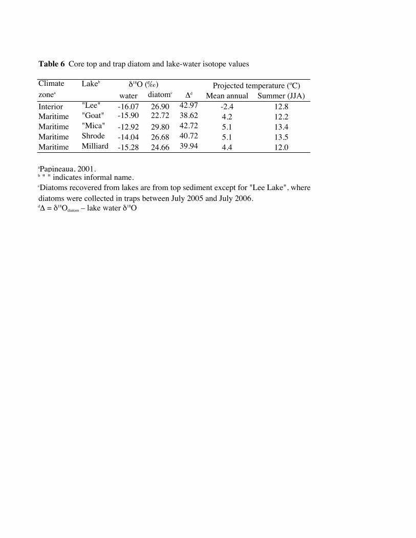
Lakeb
water diatomc!d Mean annual Summer (JJA)
Interior "Lee" -16.07 26.90 42.97 -2.4 12.8
Maritime "Goat" -15.90 22.72 38.62 4.2 12.2
Maritime "Mica" -12.92 29.80 42.72 5.1 13.4
Maritime Shrode -14.04 26.68 40.72 5.1 13.5
Maritime Milliard -15.28 24.66 39.94 4.4 12.0
aPapineaua, 2001.b " " indicates informal name.cDiatoms recovered from lakes are from top sediment except for "Lee Lake", where
diatoms were collected in traps between July 2005 and July 2006.d! = "18Odiatom – lake water "18O
Climate
zonea
Projected temperature (ºC)"18O (‰)
Table 6 Core top and trap diatom and lake-water isotope values
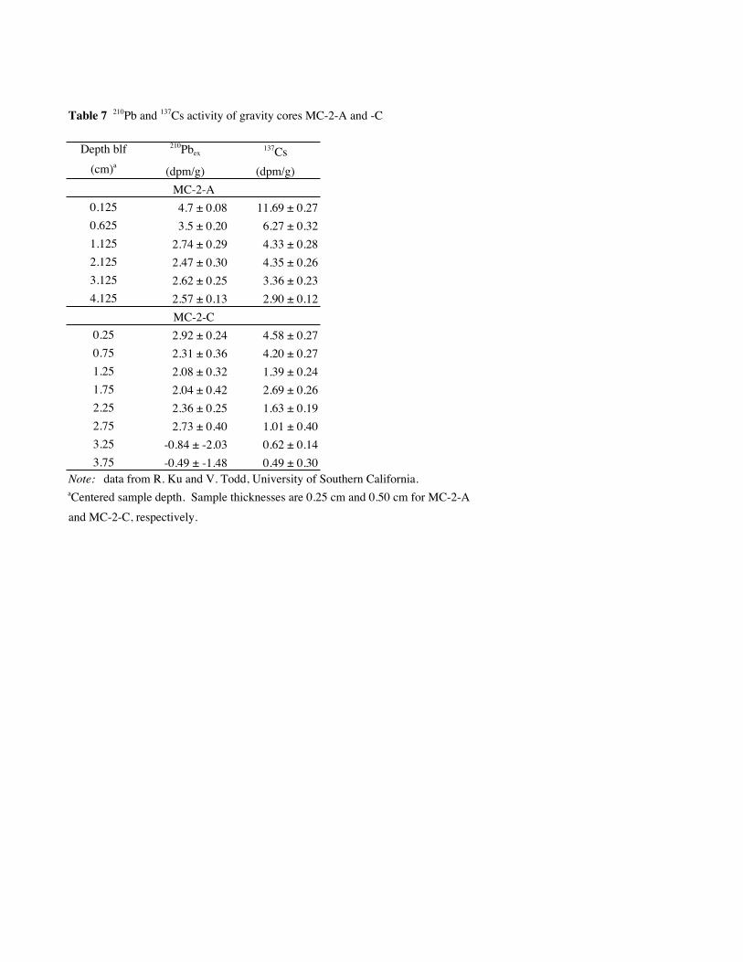
0.125
0.625
1.125
2.125
3.125
4.125
0.25
0.75
1.25
1.75
2.25
2.75
3.25
3.75
Note: data from R. Ku and V. Todd, University of Southern California.aCentered sample depth. Sample thicknesses are 0.25 cm and 0.50 cm for MC-2-A
and MC-2-C, respectively.
3.5 ± 0.20
2.74 ± 0.29
2.47 ± 0.30
2.62 ± 0.25
2.57 ± 0.13
-0.49 ± -1.48
-0.84 ± -2.03
2.73 ± 0.40
2.36 ± 0.25
2.04 ± 0.42
2.08 ± 0.32
2.31 ± 0.36
2.92 ± 0.24
MC-2-C
11.69 ± 0.27
(dpm/g)
137Cs
MC-2-A
4.7 ± 0.08
Depth blf
(cm)a
210Pbex
(dpm/g)
0.49 ± 0.30
0.62 ± 0.14
1.01 ± 0.40
1.63 ± 0.19
Table 7 210Pb and 137Cs activity of gravity cores MC-2-A and -C
2.69 ± 0.26
1.39 ± 0.24
4.20 ± 0.27
6.27 ± 0.32
4.33 ± 0.28
4.35 ± 0.26
4.58 ± 0.27
3.36 ± 0.23
2.90 ± 0.12
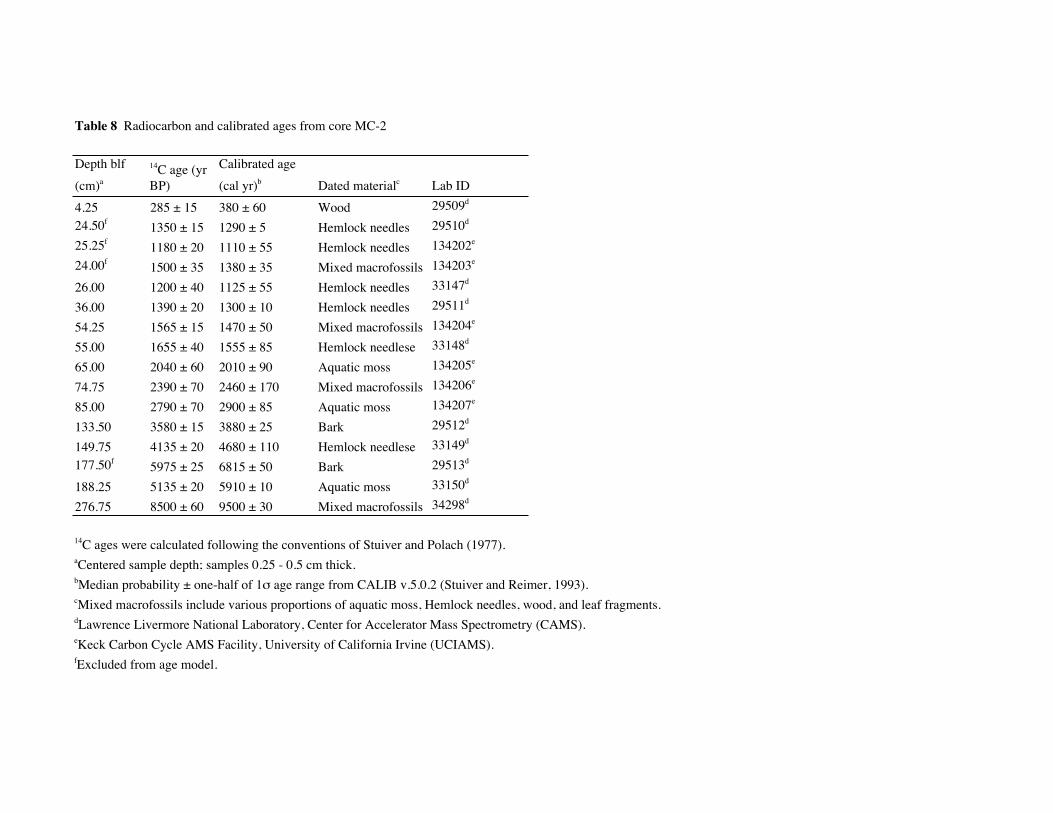
Depth blf
(cm)a
14C age (yr
BP)
Calibrated age
(cal yr)b Dated materialc Lab ID
4.25 285 ± 15 380 ± 60 Wood 29509d
24.50f1350 ± 15 1290 ± 5 Hemlock needles 29510d
25.25f1180 ± 20 1110 ± 55 Hemlock needles 134202e
24.00f1500 ± 35 1380 ± 35 Mixed macrofossils 134203e
26.00 1200 ± 40 1125 ± 55 Hemlock needles 33147d
36.00 1390 ± 20 1300 ± 10 Hemlock needles 29511d
54.25 1565 ± 15 1470 ± 50 Mixed macrofossils 134204e
55.00 1655 ± 40 1555 ± 85 Hemlock needlese 33148d
65.00 2040 ± 60 2010 ± 90 Aquatic moss 134205e
74.75 2390 ± 70 2460 ± 170 Mixed macrofossils 134206e
85.00 2790 ± 70 2900 ± 85 Aquatic moss 134207e
133.50 3580 ± 15 3880 ± 25 Bark 29512d
149.75 4135 ± 20 4680 ± 110 Hemlock needlese 33149d
177.50f5975 ± 25 6815 ± 50 Bark 29513d
188.25 5135 ± 20 5910 ± 10 Aquatic moss 33150d
276.75 8500 ± 60 9500 ± 30 Mixed macrofossils 34298d
14C ages were calculated following the conventions of Stuiver and Polach (1977).aCentered sample depth; samples 0.25 - 0.5 cm thick.bMedian probability ± one-half of 1! age range from CALIB v.5.0.2 (Stuiver and Reimer, 1993).cMixed macrofossils include various proportions of aquatic moss, Hemlock needles, wood, and leaf fragments.dLawrence Livermore National Laboratory, Center for Accelerator Mass Spectrometry (CAMS).eKeck Carbon Cycle AMS Facility, University of California Irvine (UCIAMS).fExcluded from age model.
Table 8 Radiocarbon and calibrated ages from core MC-2
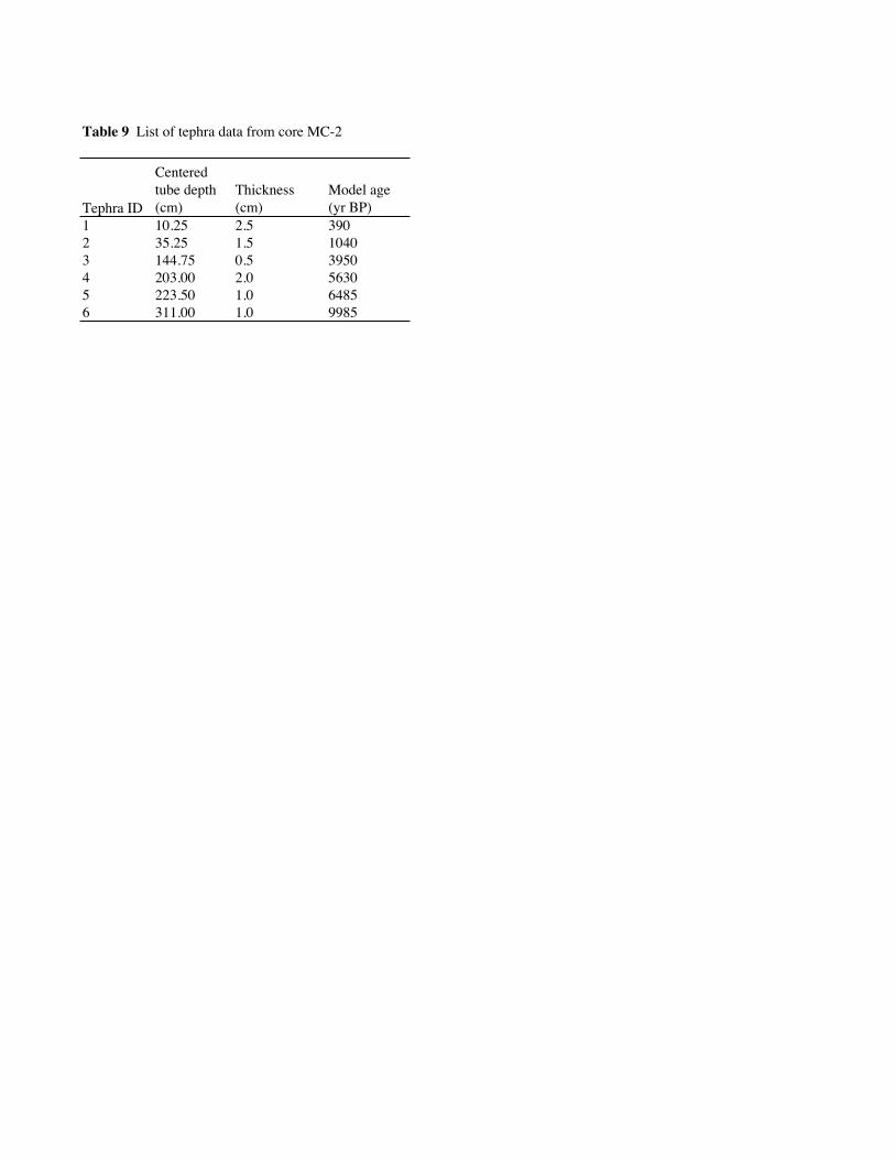
Table 9 List of tephra data from core MC-2
Tephra ID
Centered
tube depth
(cm)
Thickness
(cm)
Model age
(yr BP)
1 10.25 2.5 390
2 35.25 1.5 1040
3 144.75 0.5 3950
4 203.00 2.0 5630
5 223.50 1.0 6485
6 311.00 1.0 9985
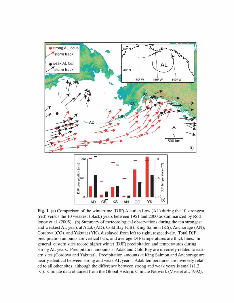
weak AL loci
storm track
strong AL locus
storm track
N
500 km
a)
AN
KS
AD
CO YK
CB
0
500
1000
DJF
pre
cip
itation (
mm
)
DJF
tem
pera
ture
(oC
)
-5
0
-10
AN YKCOCBAD KSb)
Fig. 1 (a) Comparison of the wintertime (DJF) Aleutian Low (AL) during the 10 strongest (red) versus the 10 weakest (black) years between 1951 and 2000 as summarized by Rod-ionov et al. (2005). (b) Summary of meteorological observations during the ten strongestand weakest AL years at Adak (AD), Cold Bay (CB), King Salmon (KS), Anchorage (AN), Cordova (CO), and Yakutat (YK), displayed from left to right, respectively. Total DJF precipitation amounts are vertical bars, and average DJF temperatures are thick lines. In general, eastern sites record higher winter (DJF) precipitation and temperatures during strong AL years. Precipitation amounts at Adak and Cold Bay are inversely related to east-ern sites (Cordova and Yakutat). Precipitation amounts at King Salmon and Anchorage are nearly identical between strong and weak AL years. Adak temperatures are inversely relat-ed to all other sites, although the difference between strong and weak years is small (1.2 °C). Climate data obtained from the Global Historic Climate Network (Vose et al., 1992).
AL
140º W160º W180º W
40º N
60º N

0
5
10
151900 1920 1940 1960 1980 2000
DJF NPI
15 yr movingaverage DJF NPI
NP
I val
ue (
-100
0 m
b)
Year ADFig. 2 The annual and 15 yr moving average DJF North Pacific Index (NPI) (see text for
details), which is a measure of the intensity of the Aleutian Low (AL). High NPI values
correspond to weak AL. Black vertical bars mark the three shifts of the NPI during the 20th
century at 1925, 1947, and 1976. NPI data provided by the Climate Analysis Section,
NCAR, Boulder, USA, Trenberth and Hurrell (1994).
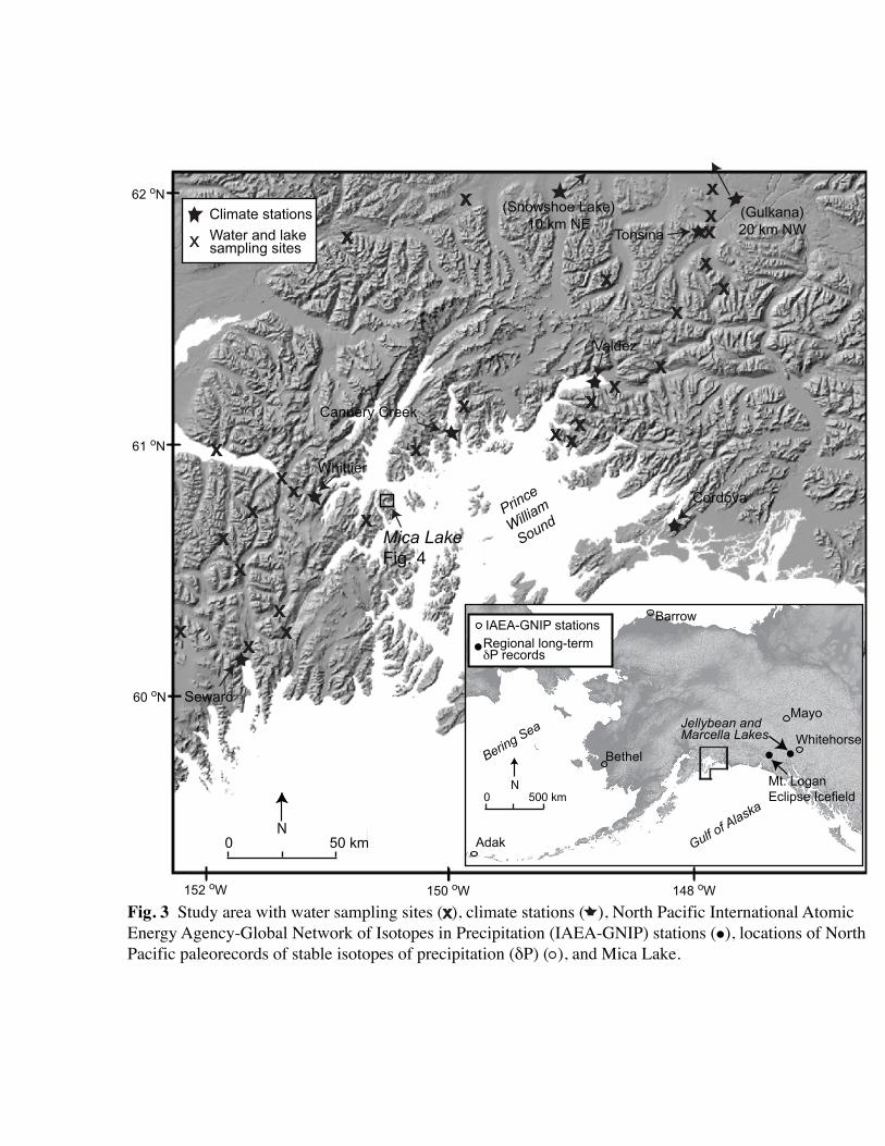
Mt. LoganEclipse Icefield
Jellybean and Marcella Lakes
Gulf of A
laska
BarrowIAEA-GNIP stations
Mayo
Bethel
Regional long-termδP records
Whitehorse
Adak
Cordova
Valdez
Whittier
Seward
(Snowshoe Lake)10 km NE
(Gulkana)20 km NWTonsina
xx
x
x
x
x xx
x
x
xx
xx
x
x
x
x
x
xxx
xx
xx
x
x
Mica LakeFig. 4
Cannery Creek
xClimate stations
Water and lake sampling sites
N0 50 km
62 oN
61 oN
60 oN
152 oW 148 oW150 oW
Prince
William
Sound
N500 km0
Bering Sea
Fig. 3 Study area with water sampling sites ( ), climate stations ( ), North Pacific International Atomic Energy Agency-Global Network of Isotopes in Precipitation (IAEA-GNIP) stations ( ), locations of North Pacific paleorecords of stable isotopes of precipitation (δP) ( ), and Mica Lake.
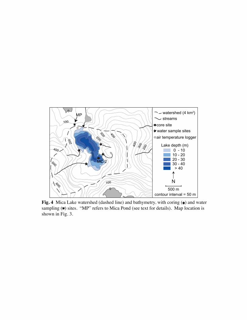
0
100
0
100
200
400
500
600
200300400
400
300200
MP
N
500 m
air temperature logger
core site
watershed (4 km2)
contour interval = 50 m
water sample sites
0 - 1010 - 2020 - 3030 - 40
> 40
Lake depth (m)
streams
MC-2
Fig. 4 Mica Lake watershed (dashed line) and bathymetry, with coring ( ) and watersampling ( ) sites. “MP” refers to Mica Pond (see text for details). Map location isshown in Fig. 3.
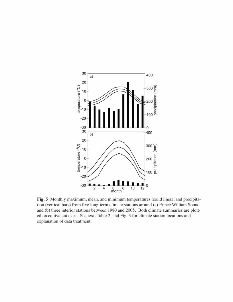
-30
-20
-10
0
10
20
30
0
100
200
300
400
prec
ipita
tion
(mm
)
tem
pera
ture
(°C
)
2 4 121086month
b)
0
100
200
300
400
-30
-20
-10
0
10
20
30
prec
ipita
tion
(mm
)
tem
pera
ture
(°C
)a)
Fig. 5 Monthly maximum, mean, and minimum temperatures (solid lines), and precipita-tion (vertical bars) from five long-term climate stations around (a) Prince William Sound and (b) three interior stations between 1980 and 2005. Both climate summaries are plott-ed on equivalent axes. See text, Table 2, and Fig. 3 for climate station locations and explanation of data treatment.

coreMC-2
Fig. 6 Flow chart illustrating the diatom isolation protocol adapted from Morley et al. (2004).
rinse x 3
chem
ical
isol
atio
n
grain size isolation
heav
y liq
uid
isol
atio
n
rinse x 3residual organics?
residual clays?
rinse x 3
visual inspection at 20X
pure
cont
amin
ated
mass-spec
50 µm
10 µm
sieve
90°C12 hr
30% H2O2
5% HCl25°C12 hr
centrifugedifferential
setting
float = diatoms
sink = clay/silt
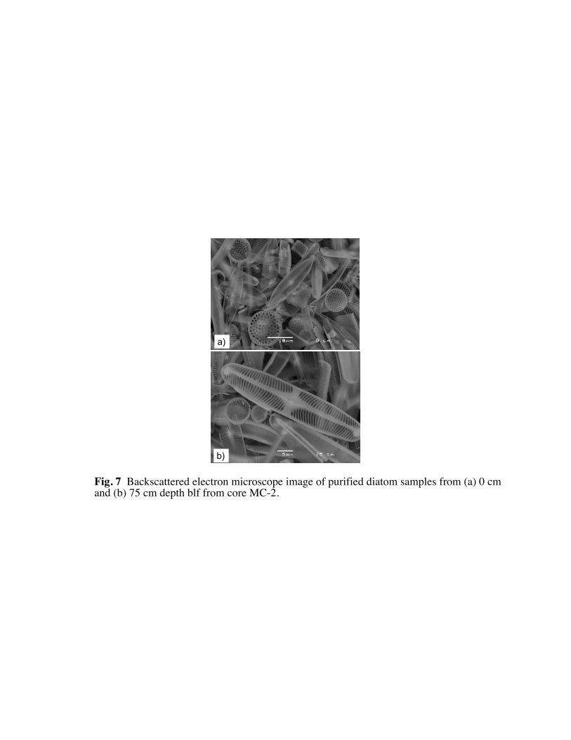
a)
b)
Fig. 7 Backscattered electron microscope image of purified diatom samples from (a) 0 cm and (b) 75 cm depth blf from core MC-2.

y = 0.84x - 0.54r2 = 0.95
-20
-10
0
10
20
-20 -10 0 10 20Whittier air temperature (°C)
Mic
a La
ke a
ir te
mpe
ratu
re (
°C)
a)
Annual
R2 = 0.76
JJA
R2 = 0.95
SON
R2 = 0.84
DJF
R2 = 0.91
MAM
0
20
40
60
80
100
6/24/06 8/13/06 10/2/06 11/21/06 1/10/07 3/1/07 4/20/07 6/9/07Date
cum
ulat
ive
annu
al p
reci
pita
tion
at M
ica
Lake
wat
ersh
ed (
%)
b)
70%
Fig. 8 (a) Daily air temperature at Mica Lake compared to Whittier, AK between 3 July 2006 and 2July 2007. Data were subdivided to calculate seasonal lapse rates used to estimate temperature at the median elevation of the Mica Lake watershed (364 m a.s.l.). Black lines are least-squares linear or power (JJA) regressions. Data available online: http://jan.nau.ucc.edu/~dsk5/S_AK/. (b) Cumulative precipitation (black line) with the days of below 0 °C daily temperatures at the median elevation of the Mica Lake watershed and precipitation received at Whittier (vertical gray lines).

-180
-140
-100
-60
-20
-24.0 -19.0 -14.0 -9.0 -4.0
a) all data
δD (
‰)
δD (
‰)
δ18O (‰) δ18O (‰)
y = 6x - 54
R2 = 0.92
-180
-140
-100
-60
-20
-24.0 -19.0 -14.0 -9.0 -4.0
d) interior
y = 6x - 36
R2 = 0.92
-180
-140
-100
-60
-20
-24.0 -19.0 -14.0 -9.0 -4.0
c) transitional
Fig. 9 Water isotope values for samples from 2006 and 2007 lake survey, south Alaska.
(a) All data with different symbols indicating different climate regimes, (b, ) PWS, (c, )
transitional, and (d, ) interior samples. Gray line is the global meteoric water line
[GMWL; δD = 8 δ18O + 10 (Dansgaard, 1964)] and gray square is Mica Lake surface water.
The slope and distance from the GMWL of the least-squares regression for each region
provides a measure of evaporative effects. Note that the PWS line is parallel to the
GMWL. δ18O and δD data reported relative to V-SMOW.
y = 8x + 13
R2 = 0.96
-180
-140
-100
-60
-20
-24.0 -19.0 -14.0 -9.0 -4.0
b) maritime
(PWS)

4
2
0
km
a.s
.l.
maritimetransitionalinterior
SN
Gulk
ana
Tonsin
a
Snow
hoe L
ake
Cannery
Cre
ek
Vald
ez
Whittier
Sew
ard
Cord
ova
δ18O = -14.6 ‰
δD = -108 ‰
d-excess = 8.4
δ18O = -19.5 ‰
δD = -149 ‰
d-excess = 5.8
δ18O = -14.8 ‰
δD = -136 ‰
d-excess = -17.9
a)
60 °N62 °N
-180
-140
-100
-60
-20
-24.0 -19.0 -14.0 -9.0 -4.0
GMWL
maritime
(PWS)
interiortransitional
δD (
‰)
δ18O (‰)b)
outflow-12.9 ‰(n = 2)
inflow
-12.7
‰(n
= 7
)
surface-12.9 ‰(n = 4)
bottom-13.3 ‰(n = 2)
MP
-8.6 ‰
(n = 1)
c)
Mica Lake60.96° N, 148.15° W100 m a.s.l.
δ18Odiatom
25.2 - 29.8 ‰
Fig. 10 (a) Summary of south Alaska water isotopes. South-to-north directed arrow
indicates general direction of regional moisture transport. Data from ( ) climate stat-
ions from maritime and interior sites are shown in Fig. 5, and locations are in Fig. 3.
δ18O, δD, and d-excess are the averages from all samples collected in each region.
Low d-excess values at interior sites reflect the departure of δW values from the GMWL
due to evaporation. (b) Summary δ18O and δD slopes for each region. Gray line is the
GMWL and gray square is the surface water at Mica Lake. The lower slope and offset
of the interior line from the GMWL confirms evaporative effects, while the parallel and
maritime line reflects local precipitation. (c) Water isotope data for samples collected
within the Mica Lake watershed. All samples collected during the summer of 2006 and
2007. “MP” refers to Mica Pond (see text for details). δ18O and δD data reported relative
to V-SMOW.

r = 0.60
p < 0.1
0
400
800
1200non-glacial lakes glacial lakes
δ18O (‰)δ18O (‰)
lake e
levation (
m)
media
n w
ate
rshed
ele
vation (
m)
δ18Odiatom
(‰)
modern diatoms
0
400
800
1200
0
400
800
1200
incre
ased e
levation
depleted δ18O
r = 0.98
p<0.1
3028262422
r = 0.95
p < 0.0001
0
400
800
1200
-20 -16 -14 -12-18
r = 0.39
p = 0.34
r = 0.66
p = 0.34
a) c)
b) d)
e)
f)
-0.76‰/100m
-1.73‰/100m
r = 0.60
p = 0.12
-20 -16 -14 -12-18
Fig. 11 Lake elevation and median watershed elevation compared with lake water isotope data (δW) for glacial and non-glacial lakes and top-sediment diatoms in the Prince William Sound (PWS). The correlations between δW and median watershed elevation (b, d, f) are stronger and more significant than with lake elevation (a, c, e).

y = 2.3(‰) + 58.9
r = 0.99, p<0.01
20
24
28
32
-17 -15 -13δ18O
water (‰)
δ18O
dia
tom (‰
)
δ18O
dia
tom (‰
)
a)
y = 5.8(°C) - 1.4
r = 0.94, p<0.1
3.5 4.5 5.5
mean air temperature (°C)
b)
(2.4°C, 26.9‰)
y = 3.1(°C) - 14.1
r = 0.87, p=0.13
20
24
28
32
11.5 12.5 13.5
JJA air temperature (°C)
c)
200 400 600 800
y = -0.0173(m) + 35.3
r = 0.98, p<0.1
d)
-1.73‰/100 m
interior
PWS
median watershed elevation (m)
Fig. 12 Relationship between modern δ18Odiatom
and a) δ18Owater
, b) mean annual air temperature (MAT), c) summer air temp-
erature (JJAT), and d) median watershed elevation from four Prince William Sound (PWS) ( ) and one interior ( ) lakes.
Dashed line in (a) shows the 1:1 fractionation between diatoms and water. Assuming a constant fractionation the observed
fractionation factor is, α = (1000 + δ18Odiatom
)/(1000 + δ18Owater
) = 1.04.

-3
0
3
6
ln21
0 Pb ex
act
ivity
(dp
m/g
)
a)
0
3
6
9
12
0 1 2 3 4Depth blf (cm)
137 C
s a
ctiv
ity (
dpm
/g)
b)
MC-2-C
MC-2-A
Fig. 13 210Pb and 137Cs profiles for gravity cores MC-2-A and -C. Data listed in Table 7.

0
1
2
3
4
5
6
7
8
9
100 50 100 150 200 250
Adjusted depth blf (cm)
Age
(ca
l kyr
BP
)
mixed effect regression (k = 7)95% confidence intervalcalibrated median probability with 2σ age rangesrejected ages
avalanche deposit
tephra depositxxx
0.8
1.0
1.2
1.4
20 30 40 50Adjusted depth blf (cm)
Age
(ca
l kyr
BP
)
xxxx
xxxx
xxxx
xx
xxxx
x
xxxx
x
xxxx
x
xxxx
x
xxxx
x
xxx
x
age overlaps with the WRA (1147 yr BP)
Fig. 14 Spline fit age model (Heegaard et al., 2005) constructed from 13 calibrated ages (see text
for details) and the age of the surface sediment (2006). The depths of each dated level was deter-
mined after subtracting the cumulative thickness of tephra and avalanche deposits. 14
C data listed
in Table 8.
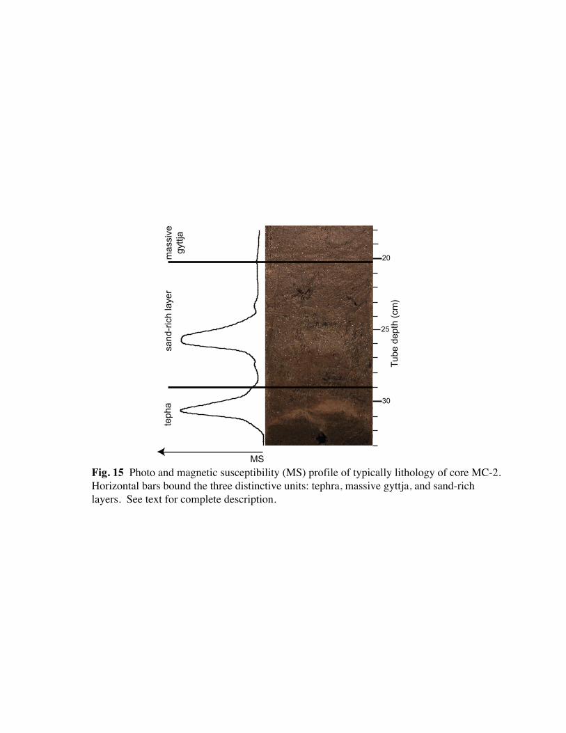
30
25
20
Tub
e de
pth
(cm
)
sand
-ric
h la
yer
teph
a
MS
mas
sive
gyttj
a
Fig. 15 Photo and magnetic susceptibility (MS) profile of typically lithology of core MC-2.
Horizontal bars bound the three distinctive units: tephra, massive gyttja, and sand-rich
layers. See text for complete description.

II
X X X X X X X X X X XX
II
I
IX X XX X X X X X X X
Unit
designation
I
II
IX X XX X X X X X X X
I
II
I
X X XX X X X X X X X
X X XX X X X X X X X
X X XX X X X X X X XI
10 Y
R, 2
/2
10 Y
R, 3
/4
Str
ata
gra
phic
log
colo
r code
massive
gyttja
(unit I)
tephras
(unit X)
7.5
YR, 3
/2
10 Y
R, 3
/2
10 Y
R, 3
/3
10 Y
R, 3
/4
sand-rich
layers
(unit II)
7.5
YR, 5
/0
10 Y
R, 3
/4
Expla
nation
0 250
MS (x 10-5 SI)
Tube d
epth
(cm)
0
100
200
300
Depth
blf
(cm)
0
100
200
312 287
250
250
150
150
50
50
r = 0.52
0
10
20
30
40
0 2 4 6 8
BSi (%)
OM
(%
)
25
26
27
28
29
30
0 2 4 6 8
δ18O
dia
tom (
‰)
BSi (%)
25
26
27
28
29
30
0 10 20 30 40
OM (%)
δ18O
dia
tom (
‰)
*
*
*
*
*
*
*
*
*
*
*
*
**
*
*
0
1
2
3
4
5
6
7
8
9
10
Age
(kyr BP) 0.0 4.0 8.0
BSi (%)MC-2-C
Lake floorMC-2
0 20 40
OM (%)
24 26 28 30
δ18Odiatom
(‰)
* included 14C age
* excluded 14C age
Fig. 16 Geochemical, physical, and chronological summary for core MC-2. The depth below lake floor (blf) is the adjusted of tube depth after adding the
thickness of core top that was lost from the percussion core, but recovered in the surface core, and removing the thickness of the tephra and avalanche
deposits. Physical and geochemical analyses include magnetic susceptibility (MS), organic matter content (OM), biogenic silica (BSi), and diatom oxygen
isotopes (δ18Odiatom
). Error bars for δ18Odiatom
determined from duplicate analyses from 10 horizons and range from 0.0 to 0.5 ‰. Distinct sediment types
include: tephra (X), massive gyttja (I), and sand-rich layers (II). δ18Odiatom
reported relative to V-SMOW.

Age (
kyr
BP
)
1
2
3
4
5
6
7
8
9
10
026 28 30
δ18Odiatom
(‰)
weak strongAleutian Low
zonal meridionalFlow Regime
west southSource
a)
-17-19-21
δ18Oca
(‰)
b)
-38 -34 -30 -26
δ18Oice
(‰)
c)
Sourcesouthnorth
Flow Regimemixedzonal
strongweakAleutian Low
Fig. 17 Oxygen isotope records from (a) Mica Lake diatoms compared to other North
Pacific δ18O records from (b) Jellybean Lake carbonate (Anderson et al., 2005) and (c)
Mt. Logan ice cores. The inferred influences of climatic controls discussed in the text
are indicated. The climatic interpretations suggested from model simulations by Fisher
et al. (2004) explain the variability at Jellybean Lake and Mt. Logan. The Mica Lake
and Mt. Logan δ18O data are reported relative to V-SMOW, whereas Jellybean Lake δ18O
data reported relative to V-PDB.

32
30
28
26
24
δ18Odiatom
0
5
10
151900 1920 1940 1960 1980 2000
DJF NPI15 yr movingaverage DJF NPI
NP
I valu
e (
-1000 m
b)
Year AD
δ18O
dia
tom
(‰
)
first-order
DJF NPI trend
Fig. 18 The 20th century δ18Odiatom
values from Mica Lake plotted with the North Pacific
Index (NPI). NPI data same as Fig. 2 but with the linear regression (dashed line) fit to
emphasize first-order trend. The Mica Lake δ18O data reported relative to V-SMOW.

Appendix A-1. Magnetic susceptibility data for core MC-2-C
Tube
depth 0 20
0.0 36 19
0.5 35 20
1.0 37 22
1.5 38 28
2.0 38 33
2.5 37 36
3.0 20 49
3.5 12 45
4.0 16 44
4.5 23 38
5.0 20 51
5.5 23 71
6.0 16 120
6.5 16 82
7.0 17 72
7.5 20
8.0 39
8.5 56
9.0 67
9.5 123
10.0 150
10.5 133
11.0 129
11.5 47
12.0 18
12.5 7
13.0 6
13.5 5
14.0 4
14.5 7
15.0 7
15.5 6
16.0 2
16.5 5
17.0 10
17.5 15
18.0 17
18.5 17
19.0 18
19.5 18Note: The sums of the column and row headings indicate the depth in cm for the magnetic
susceptibility readings. Magnetic susceptibility reported in 10-6 SI units.

Appendix A-2. Magnetic susceptibility data for core MC-2
Tube
depth 0 20 40 60 80 100 120 140 160 180 200 220
0.0 23 49 2 7 1 5 9 6 10 54 10 5
0.5 26 47 4 5 1 7 10 7 11 63 10 8
1.0 24 45 3 3 1 6 10 6 8 70 11 8
1.5 27 52 0 2 1 6 10 6 11 72 11 11
2.0 48 75 -1 1 0 6 9 8 4 83 13 12
2.5 106 66 -1 -1 1 7 8 15 3 89 14 12
3.0 115 167 1 -1 1 7 6 12 3 91 15 14
3.5 94 341 1 1 1 6 1 7 3 75 16 13
4.0 82 629 3 1 2 6 2 8 5 86 15 15
4.5 109 627 6 1 4 7 16 9 5 87 16 15
5.0 115 178 7 0 1 10 16 10 5 84 14 17
5.5 53 79 7 4 5 10 23 12 8 81 17 19
6.0 12 69 6 9 5 11 23 12 12 112 10 19
6.5 8 48 7 34 5 11 21 13 16 98 6 23
7.0 6 48 8 82 5 10 23 12 19 105 6 25
7.5 8 100 7 128 5 12 22 15 21 153 7 20
8.0 8 172 8 27 5 11 22 15 11 163 6 21
8.5 7 430 8 13 6 13 24 14 7 156 6 25
9.0 9 648 5 4 6 20 23 13 6 126 7 22
9.5 14 189 7 2 6 15 27 13 6 106 7 23
10.0 17 73 8 2 8 15 29 14 6 77 11 23
10.5 17 6 7 3 6 7 28 15 6 65 17 22
11.0 17 4 7 2 1 4 22 20 10 69 20 12
11.5 20 2 6 2 1 4 29 18 13 63 24 8
12.0 21 2 7 2 2 2 27 19 17 32 31 7
12.5 23 2 9 1 1 2 23 19 24 38 25 8
13.0 25 2 10 2 1 3 38 20 12 20 18 9
13.5 19 2 9 2 1 3 52 16 7 9 15 10
14.0 21 2 10 2 0 3 35 12 9 40 15 9
14.5 21 2 10 2 0 3 33 16 12 57 25 9
15.0 22 1 8 3 -1 5 29 20 17 62 31 12
15.5 25 2 13 4 1 5 17 20 19 108 33 11
16.0 26 1 10 4 0 3 37 28 24 170 -2 11
16.5 30 1 13 4 1 3 27 21 27 229 41 14
17.0 36 1 17 5 0 5 5 12 33 261 123 17
17.5 37 1 14 2 1 7 5 8 38 303 64 20
18.0 41 0 13 4 1 9 13 8 42 64 15 25
18.5 47 0 15 3 1 10 29 8 42 19 8 18
19.0 54 -1 24 3 3 11 35 8 45 14 6 19
19.5 50 2 19 1 4 10 9 7 47 11 4 17Note: The sums of the column and row headings indicate the depth in cm for the magnetic
susceptibility readings. Magnetic susceptibility reported in 10-6 SI units.
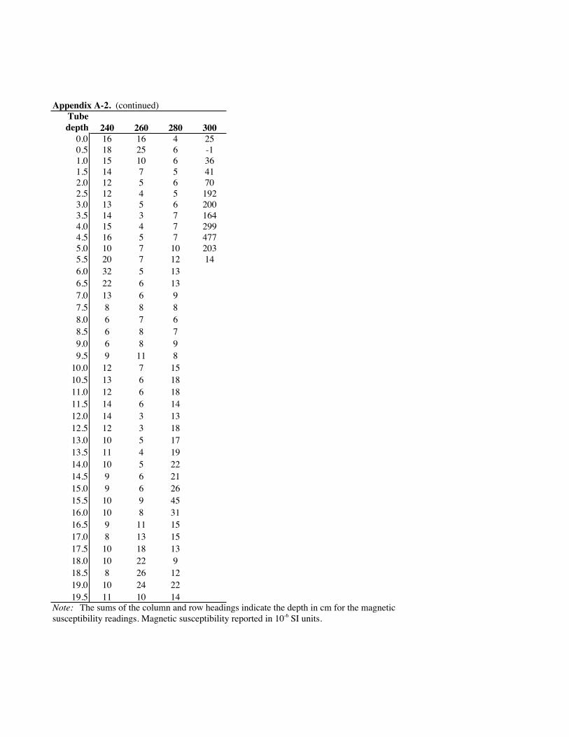
Appendix A-2. (continued)
Tube
depth 240 260 280 300
0.0 16 16 4 25
0.5 18 25 6 -1
1.0 15 10 6 36
1.5 14 7 5 41
2.0 12 5 6 70
2.5 12 4 5 192
3.0 13 5 6 200
3.5 14 3 7 164
4.0 15 4 7 299
4.5 16 5 7 477
5.0 10 7 10 203
5.5 20 7 12 14
6.0 32 5 13
6.5 22 6 13
7.0 13 6 9
7.5 8 8 8
8.0 6 7 6
8.5 6 8 7
9.0 6 8 9
9.5 9 11 8
10.0 12 7 15
10.5 13 6 18
11.0 12 6 18
11.5 14 6 14
12.0 14 3 13
12.5 12 3 18
13.0 10 5 17
13.5 11 4 19
14.0 10 5 22
14.5 9 6 21
15.0 9 6 26
15.5 10 9 45
16.0 10 8 31
16.5 9 11 15
17.0 8 13 15
17.5 10 18 13
18.0 10 22 9
18.5 8 26 12
19.0 10 24 22
19.5 11 10 14Note: The sums of the column and row headings indicate the depth in cm for the magnetic
susceptibility readings. Magnetic susceptibility reported in 10-6 SI units.

Depth BSi OM
(blf) (%) (%) run 1 run 2 AVG
0.25 4.9 14 29.8
0.75 6.4 14 28.6
1.25 4.5 12 28.4
1.75 4.4 12 27.0
3.25 5.0 22 25.9 25.7 25.8
3.75 4.8 19 26.2 25.9 26.0
4.25 4.7 14 27.3
4.75 5.0 16 27.4
5.25 4.6 17 27.3
12.75 5.5 18 29.2
13.25 6.4 20 29.0
13.75 5.7 20 28.7
14.75 5.4 19 28.1
15.75 5.1 18 27.6
16.75 5.2 15 29.0
22.75 4.0 9 26.5
24.25 1.7 15 28.4
29.25 6.5 27 26.1
39.25 6.4 20 25.5
44.25 5.9 20 28.7
49.25 5.1 21 28.2 28.2 28.2
54.25 5.1 32 28.7 28.5 28.6
59.25 7.2 27 27.5
64.25 5.5 26 28.2 28.3 28.3
69.25 7.1 25 27.1
74.25 5.4 25 25.6 24.9 25.2
79.25 6.0 25 29.4 28.7 29.1
89.25 5.1 35 28.9 28.7 28.8
99.25 5.8 18 28.0
109.25 6.1 29 28.0
119.25 5.3 16 28.4
129.25 3.5 19 28.7
138.75 7.2 21 29.0 28.9 29.0
149.75 4.3 17 28.6
168.75 5.2 16 28.5
178.75 3.4 8 28.5
180.25 3.3 5 28.4
188.25 6.2 16 29.0
198.25 5.0 18 29.6
207.25 4.7 15 28.0 28.0 28.0
217.25 4.7 16 28.6
227.25 4.5 14 27.4
247.25 4.6 18 28.1
257.25 5.8 18 29.4
266.75 6.3 19 28.3
276.75 5.1 11 29.0Note: Centered depth of 0.5-cm-thick samples. Isotope values reported vs. V-SMOW.
!18Odiatom (‰)
Appendix B-1. Biogenic silica (BSi), organic matter (OM), and diatom oxygen isotope (!18Odiatom) data for core MC-2