a modern compressible flow laboratory experience for ...arc.uta.edu/publications/cp_files/aiaa...

A Modern Compressible Flow Laboratory Experience

for Undergraduates

Frank K. Lu,∗ Sikander Ali,† Eric M. Braun,‡ and Luca Maddalena§

University of Texas at Arlington, Arlington, Texas, 76019

Two experiments involving compressible flow, namely, unsteady flow in a shock tubeand expansion in a freejet, are described. The latter includes experience in numericalsimulations. These laboratory experiences reinforce classroom instruction and serve anumber of learning goals. By including simulations and a simple inviscid model, the datafrom the freejet experiments can be validated and verified. Such a process is increasinglyimportant for engineers.

I. Introduction

AWELL-DEVELOPED laboratory experience is an important aspect of any undergraduate engineeringcurriculum, including aerospace engineering. The aerospace laboratory follows a basic measurements

course which typically includes digital data acquisition techniques, instrumentation, data processing andelementary statistics. At the authors’ institution, the basic sophomore measurements course is then followedconsecutively by an aero-structures and an aerodynamics laboratory in the fall and spring semesters ofthe junior year. The students by the spring semester of the junior year will have taken an incompressibleaerodynamics course. They will be enrolled in the compressible aerodynamics course concurrently with theaerodynamics laboratory. Thus, a compressible laboratory experience in the same semester will help toreinforce classroom instruction.

Unlike the basic measurements course, reinforcing classroom instruction imposes a different set of objec-tives for the aerodynamics laboratory. A critical objective is to ensure that students understand the physicsof the flow which is in all likelihood more complicated that the idealizations introduced in the classroom.Thus, a part of this objective is to allow the students to perform a critical evaluation of inviscid theory.For example, the presence of shocks in a nozzle induces boundary layer separation will likely not be wellexplained in class. Nonetheless, it is important to ensure that the students are aware of the limitations ofinviscid theory in situations where viscous effects are important.

A separate challenge which may have not been well addressed in laboratory development is exposingstudents to modern engineering software tools. Some may argue against introducing such tools in an academicenvironment for fear that these tools defeat the learning process. Others argue that software can misleadstudents into thinking that these tools can solve problems and lull them into a sense of complacency wherethe danger of erroneous results are not appreciated and thus “sanity” checks are not made. Nonetheless, a

∗Professor and Director, Aerodynamics Research Center, Department of Mechanical and Aerospace Engineering, Box 19018.Associate Fellow AIAA.

†Undergraduate Research Assistant, Aerodynamics Research Center, Department of Mechanical and Aerospace Engineering,Box 19018. Student Member AIAA.

‡Graduate Research Associate, Aerodynamics Research Center, Department of Mechanical and Aerospace Engineering, Box19018. Student Member AIAA.

§Assistant Professor, Aerodynamics Research Center, Department of Mechanical and Aerospace Engineering, Box 19018.Member AIAA.

1 of 12

American Institute of Aeronautics and Astronautics

49th AIAA Aerospace Sciences Meeting including the New Horizons Forum and Aerospace Exposition4 - 7 January 2011, Orlando, Florida

AIAA 2011-274

Copyright © 2011 by the American Institute of Aeronautics and Astronautics, Inc. All rights reserved.

well-controlled use of software, as we propose here, can help to reinforce certain skills, such as the need forsanity checks: the so-called validation and verification. Thus, the laboratory environment may be an excellentone for integrating experiment, modeling and theory, an approach that is increasingly expected in modernengineering practice. Finally, once some experience is gained, software tools help greatly in engineeringdesign. Toward this goal, the commercial fluids solver, FLUENT r©, is introduced into the aerodynamicslaboratory experience.

To meet the objectives of (i) improving the understanding of compressible flow, (ii) application of theory toexperiment, (iii) validation and verification, and (iv) use of software, two compressible flow experiments weredeveloped. Other secondary objectives include typical ones of an experimental course, such as understandingthe characteristics of instruments, data acquisition, data analysis, including uncertainty analysis, and reportwriting.

The two experiments are based on a shock tube for teaching unsteady compressible flow and a supersonicnozzle/free jet with its inherent versatility. The shock tube is easy and inexpensive to develop, usingmostly off-the-shelf components with a minimum amount of machining. The nozzle can be used to studyunderexpanded, perfectly expanded and overexpanded free jets. It can also be used to study nozzle off-design performance at low Mach number, with internal shocks inducing boundary layer separation. Thenozzle experiment is complemented with numerical simulations. The nozzle was deliberately constructedwith a rectangular cross section so that it can be operated as a miniature supersonic tunnel. Thus, smallmodels can be mounted in the test section to provide further experiences. The nozzle experiment is moreelaborate and expensive, even though every effort was made to use off-the-shelf components.

II. Implementation

The shock tube and the free jet facilities are housed in a research laboratory. While these facilities occupysome space, the execution of the experiments has a minimal impact on research activities. The experimentstake up only two weeks, requiring preparation by the teaching assistants and the laboratory technician.The preparations include checking the instrumentation, ensuring that all plumbing and wiring are workingproperly. The experiments also require the temporary use of data acquisition systems that would otherwisebe used for research, and require checking that the data acquisition programs are operating properly. Thesechecks may require a test run or two ahead of the actual laboratory sessions. Due to safety concerns, theselaboratories are operated by the teaching assistants.

A. Shock Tube

Specific objectives of this experiment are

• To develop an understanding of unsteady wave processes in a gas,

• To compute the shock Mach number from experimental data and compare against theory.

The shock tube experiment can be set up with low cost and ease, with a small amount of machining.Even though unsteady wave processes are not covered in the present classroom curriculum, this experimentprovides exposure to compressible phenomena. It also provides understanding of shock and expansion pro-cesses, with the noteworthy distinction that compression can occur over a steep front, namely, a shock,whereas expansion is an isentropic process that occurs over an extended distance.

1. Facility Description

The shock tube is shown schematically in Fig. 1(a) and a photograph is shown in Fig. 1(b). It consistsof a high-pressure, driver section (right side) and a low-pressure, driven section (left side), both made ofseamless, commercial steel pipe with an internal diameter of 1 in. The driver and driven tubes are 20 in.

2 of 12


and 28 in. long, respectively. While the driver tube is capped at its end, the driven tube is operated eithercapped or open to the ambient. Connecting the two tubes is a double diaphragm section, also made of steel.It is a 2-in. chamber. Diaphragms made of kitchen foil are placed on either side of the chamber. Next,the flanged ends of the driver and driven tubes are bolted to the double diaphragm section. A tight sealis obtained by including O-rings on the flange faces. The double diaphragm section makes it easy and safeto operate the shock tube. High-frequency pressure transducers (PCB Model 111A24) are mounted alongthe sides of the driver and driven tubes at a spacing of 4 in. Transducers are also mounted onto the endflanges of these tubes. The transducers are rated for a maximum pressure of 1000 psi. Although the 1000psi rating is far above what was measured with this experiment, the high pressure transducers were selectedfor their ruggedness since the aluminum foil diaphragms usually burst into fragments during operation. Theshock tube is shown schematically in Fig. 1(a) and a photograph is shown in Fig. 1(b). It consists of a high-pressure, driver section (right side) and a low-pressure, driven section (left side), both made of seamless,commercial steel pipe with an internal diameter of 1 in. The driver and driven tubes are 20 in. and 28 in.long, respectively. While the driver tube is capped at its end, the driven tube is operated either capped oropen to the ambient. Connecting the two tubes is a double diaphragm section, also made of steel. It is a2-in. chamber. Diaphragms made of kitchen foil are placed on either side of the chamber. Next, the flangedends of the driver and driven tubes are bolted to the double diaphragm section. A tight seal is obtainedby including O-rings on the flange faces. The double diaphragm section makes it easy and safe to operatethe shock tube. High-frequency pressure transducers (PCB Model 111A24) are mounted along the sidesof the driver and driven tubes at a spacing of 4 in. Transducers are also mounted onto the end flanges ofthese tubes. The transducers are rated for a maximum pressure of 1000 psi. Although the 1000 psi ratingis far above what was measured with this experiment, the high pressure transducers were selected for theirruggedness since the aluminum foil diaphragms usually burst into fragments during operation.

(a) Schematic of the shock tube along with the pres-sure transducer and filling arrangement.

(b) Photograph of shock tube.

Figure 1. Shock tube.

Figure 1(a) shows the vents used both for safety anddraining the intermediate section pressure. Intermediateand high-pressure lines are labeled by IP and HP respec-tively. High and intermediate pressure air are broughtinto the tube sections with solenoid valves manually trig-gered from the control room. The bank of solenoid valvesis visible in the lower right of Fig. 1(b). The air is reg-ulated so the IP fills first. Next, the HP is switched on.A third solenoid valve is used to vent the IP section tocause the double diaphragms to burst. A fourth solenoidvalve is available to vent the HP section if necessary. Thehigh-pressure air is introduced to the shock tube from a175 psi compressor.

2. Test Protocol

As mentioned above, preparation for the laboratory in-cludes instrumenting the shock tube with pressure trans-ducers and connecting them to a high-speed data acquisi-tion system with a LabVIEW r© interface. Groups of 4–6students witness the experiment from a control room.

Aluminum foil is placed on both sides of the double di-aphragm section. The driver and driven sections are thenbolted to the double diaphragm section, ensuring thatthere is a good seal between the sections. The diaphragmfor this laboratory is constructed of several aluminum foillayers such that it will burst for a Δp of 110–130 psi. The

3 of 12


intermediate, double-diaphgram section can be filled with air to 60 psig initially, which the diaphragms willsafely hold. When the driver section is then filled to 150 psig, the Δp values across each diaphragm arestill below their burst limit. The intermediate section is then exhausted quickly by activating a pressurerelief vent. Activation of the vent causes Δp to rise sufficiently to burst the diaphragms. Bursting of thediaphragms starts the unsteady wave process in the shock tube. Before the vent is actuated, the DAQ andLabVIEW r© program are started with an analog trigger that waits for a pressure rise of about 10 psi intransducer P7. Data are acquired for a half second. A similar experiment is performed with the driven tubeuncapped.

3. Project Requirements

Data from the experiment are stored in EXCEL files for the students to analyze. Examples of the plotteddata collected at a 100 kHz/channel, simultaneous sampling rate are shown in Fig. 2. The students arerequired to determine the time-of-flight τ from the data. Here, they will understand the practical difficultiesof resolving a step pressure rise due to transducer size, sampling rate and noise. Once τ is determined, giventhe transducer spacing of x, the shock propagation speed and the Mach number can be computed:

us = x/τ (1)Ms = us/a1 (2)

where the speed of sound a1 =√

γRT1. Students are required to perform an uncertainty analysis on theirestimate of us and Ms since these values can be calculated 5–6 times depending on the mode of operation.The students also estimate the pressure ratio across the propagating shock p2/p1 which is an importantparameter in shock tube performance. This pressure ratio is in fact related to the shock Mach number:

Ms =

√γ + 12γ

(p2

p1− 1

)+ 1 (3)

Therefore, a separate calculation of Ms is obtained. The students also have to perform an uncertainty

(a) Sample data with open driver tube. (b) Sample data with closed driver tube.

Figure 2. Example of shock tube data.

analysis here, which is a little bit more involved. From the shock pressure ratio, the students can back

4 of 12


calculate the initial pressure ratio.

p4

p1=

p2

p1

{1 − (γ − 1) (p2/p1 − 1)√

2 γ [2 γ + (γ + 1) (p2/p1 − 1)]

}−2 γ/(γ−1)

(4)

The students are required to compare their computed value of p4/p1 against the measured one and commenton the results. The procedure is undertaken for the two test cases: open and closed end. The time-of-flightcalculations are usually associated with an uncertainty of less than 10% of the value. However, uncertaintyin the p2/p1 estimate and its associated p4/p1 and Ms values usually is greater than 10%. Comparing thesecalculation procedures and making a determination why one may be better to use over another reflectssituations that will often be encountered by a practicing engineer.

Finally, the students construct an x–t diagram with the closed end data for the incident shock and thefirst reflection. The uncertainty from the wave speeds is also indicated in the diagram. If any errors aremade while calculating the shock speed and its uncertainty, they should be obvious in the diagram and allowthe student to see where errors have been made.

B. Free Jet

(a) Schematic of supersonic freejet facility.

(b) Photograph.

Figure 3. The supersonic free jet.

Specific objectives of this experiment are

• To understand the operation of a supersonicnozzle with a constant backpressure (or vari-able supply pressure)

• To observe the formation of an underex-panded, perfectly expanded and overexpandedfree jet, including the wave patterns that arenot ideal but regularly occur in practice.

• To observe shock formation in a severely over-expanded jet

To fulfill these objectives, a small facility featur-ing a nominal Mach 2, convergent-divergent nozzlewas developed. This nozzle exhausts to the ambientwhich allows for observations of the freejet.

1. Design

The supersonic wind tunnel for the undergradu-ate laboratory experience was designed with severalconsiderations. First, the students should have ex-posure to all of the different flow regimes that occurwhile the pressure ratio is varied between the stag-nation and ambient conditions of the converging-diverging (CD) nozzle. The recognizable under- andover-expanded regimes with their shock diamondpatterns can be readily visualized. A pressure scan-ner is used to measure the pressure in taps located along the nozzle contour. The tunnel sections leadingup to the nozzle were deliberately sized such that a simple regulator could be used to control the plenumpressure. This arrangement proved to work well and obviated the need for a more elaborate control valveand large settling chamber.

5 of 12


The nozzle Mach number was arbitrarily selected to be 2. The selected run time was 20–30 s. This ismore than adequate for gathering data from the pressure scanner and for obtaining schlieren movies. Thenozzle throat is 1.4 in. high × 0.6 in. wide. This rectangular cross-section design allowed for the walls of thenozzle to be constructed of Lexan sheets for further flow visualization.a The height of the nozzle increasesto 2.36 in. which matches with the size of the in-house schlieren system.1

The CD nozzle was designed using the method of characteristics without boundary layer corrections. Oneof the goals of the laboratory is to help students understand the importance of viscous effects that will causea reduction of both the area ratio and the Mach number. After the area expansion, the nozzle contains astraight section which could be prepared in the future for inserting test articles. The bottom nozzle contourhas 16 ports with a diameter of 0.0465 in. for use with a 16-channel, Esterline 9116 pressure scanner. Elevenports are placed in the throat section to measure the pressure variation with area, and five ports are locatedin the test section.

A blowdown type, free jet tunnel configuration satisfies all of the criteria above for testing the nozzle.Run times can be predicted using a simple approach outlined by Pope and Goin2 so as to size the storagetube. A storage tank with a 50 ft3 volume and 400 psig pressure limit was selected for this facility.

The required pressure ratio for perfect expansion is p0/p∞ = 7.84, so p0 must be set to at least 115 psia.A Jordan Valve Mark 60 sliding gate regulator that can maintain up to p0 = 175 psia was chosen for thisfacility. The facility is started with a Granzow high mass flow solenoid valve. A schematic, not to scale, isshown in Fig. 3(a). The storage tank, filled by a 2000 psi compressor source, is connected to the sliding gatevalve via a 2-in. high-pressure hose. Pipe sections connect to the valves up to the flow spreader location. Atthat location, a flange assembly was designed to connect the pipe to a 2.5 × 2.5 in. square section.

A flow spreader containing 24 radial ports that send air into a plenum chamber up to the nozzle throat, ascan be seen in Fig. 3(a). Immediately downstream of the flow spreader are three 12-in. long flanged sections,each of which contains a mesh screen to reduce turbulence. The mesh sizes are 30, 40 and 50 with a solidityof about 45%. From the area ratio of the plenum chamber to the throat, air speed in the plenum chamber isless than 100 ft/s, which essentially means that stagnation conditions are upheld. The small flanged sectionbetween the last screen and the nozzle reduces the cross-sectional area from 2.5 × 2.5 in. to 2.5 × 0.6 in.

2. Simulation and Analytical Requirements

To expand the learning experience from merely experimental observations, the students will be exposed to aguided experience in using FLUENT r© for flow simulation. The students enrolled in this course are presumedto have no experience with computational fluid dynamics. Consequently, the simulation given to the studentsto work with is finished with the exception of the commands that must be entered into FLUENT r© to start asolution. Such an assignment may be considered a “canned” one because simply running it may not enhancebasic understanding of computational fluid dynamics algorithms.3

There are several reasons why running the program as part of this laboratory assignment can be a goodeducational experience. First, students can understand how to use CFD to properly support experimentalresults (and vice versa). After running the FLUENT r© program for several different stagnation pressurevalues, the pressure distribution along the centerline can be extracted to map p/p0 for all of the flowconditions that can occur with a CD nozzle.4 Figure 4(c) shows several of these conditions. The pressuredistribution from the nozzle wall can also be matched with the pressure scanner data.

A second educational outcome from incorporating numerical simulation is to help develop an ability tounderstand any limits that exist with the FLUENT r© model as compared to the experiment. The gridspacing has been left coarse so each solution converges in a few thousand iterations. Consequently, theshock and expansion wave patterns seen in the experiments cannot be replicated with this model. Even withfiner grid spacing, the two-dimensional nozzle model can differ significantly from three-dimensionality in theexperiment.

aSubsequent schlieren visualization revealed stress patterns in tightening the Lexan walls. These walls will be replaced byschlieren-quality glass.

6 of 12


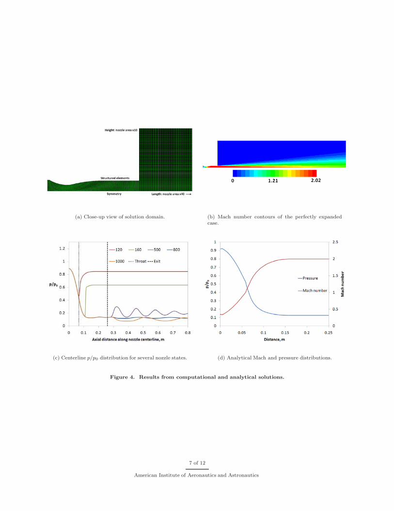
(a) Close-up view of solution domain. (b) Mach number contours of the perfectly expandedcase.

(c) Centerline p/p0 distribution for several nozzle states. (d) Analytical Mach and pressure distributions.

Figure 4. Results from computational and analytical solutions.

7 of 12


Figure 4(a) shows a partial view of the solution domain. In order for the free jet simulation to convergeproperly, the length of the domain is about 20 times larger than the nozzle exit area (after accountingfor the symmetry condition along the nozzle centerline). The pressure inlet, pressure outlet, and wallboundary conditions are used for the rest of the solution domain. About 40,000 structured cells are used,whereby overall size increases away from the nozzle and predicted exit plume location. A density-based,implicit, two-dimensional planar solution method is used. A standard k–ε viscous model is used withthe constants provided by FLUENT r© along with first-order upwind discretization. Other techniques couldclearly be utilized for a more accurate solution, but they are not necessary for the current learning objectives.The students are given step-by-step instructions for setting boundary conditions, initializing the solution,monitoring convergence, and collecting results. Convergence is considered to be reached when the drag onthe nozzle wall becomes constant along with residual values of 1e–6 or less.

Figure 4(d) shows the analytical solution for p/p0 and M in the nozzle using isentropic flow equations.

p0

p=

(1 +

γ − 12

M2

)γ/(γ−1)

(5)

A(x)A∗ =

1M

[2

γ + 1

(1 +

γ − 12

M2

)](γ+1)/2(γ−1)

(6)

In the isentropic equations, the geometry of the nozzle is used to first calculate the area ratio along thenozzle A(x)/A∗. The pressure ratio and Mach number are then computed using an iterative process for eachpoint specified along the nozzle.

3. Experimental Results

The tunnel and data collection program are initiated by the teaching assistants from the control room. Asfor the shock tube experiment, groups of 4–6 students witness the experiment. Once the storage tank hasbeen filled, the solenoid valve is simply switched on to start. The schlieren system and video camera can beturned on during the filling process. Once the nozzle is started, the regulator valve holds reasonably steadypressure for about 10 s. This pressure is held high enough such that the nozzle will remain overexpandedduring that time. Once the regulator can no longer hold constant pressure, the pressure of the storage tankas it drains is essentially the stagnation pressure. Such behavior is typical of blow-down wind tunnels, andthe control valve is usually shut at this point to conserve air. In the present case, it is left open and thenozzle progresses through all of the states based on pressure ratio.

Figure 5. Storage tank and regulator/plenum pressures during a typical test.

8 of 12


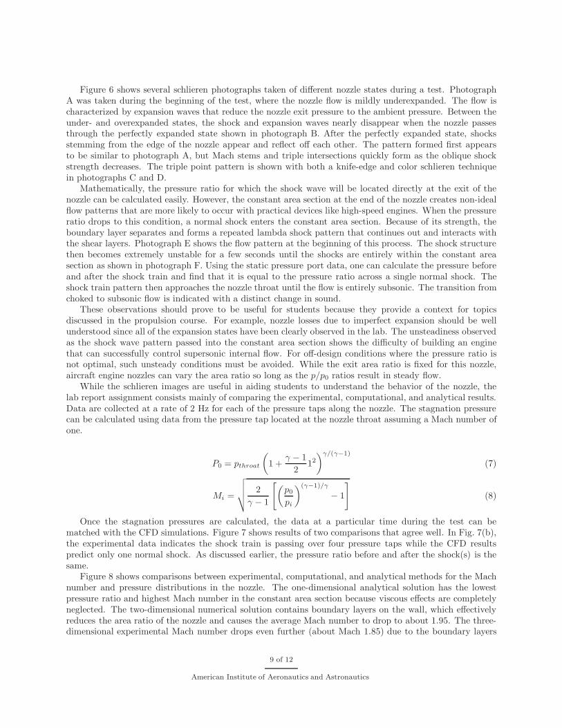
Figure 6 shows several schlieren photographs taken of different nozzle states during a test. PhotographA was taken during the beginning of the test, where the nozzle flow is mildly underexpanded. The flow ischaracterized by expansion waves that reduce the nozzle exit pressure to the ambient pressure. Between theunder- and overexpanded states, the shock and expansion waves nearly disappear when the nozzle passesthrough the perfectly expanded state shown in photograph B. After the perfectly expanded state, shocksstemming from the edge of the nozzle appear and reflect off each other. The pattern formed first appearsto be similar to photograph A, but Mach stems and triple intersections quickly form as the oblique shockstrength decreases. The triple point pattern is shown with both a knife-edge and color schlieren techniquein photographs C and D.

Mathematically, the pressure ratio for which the shock wave will be located directly at the exit of thenozzle can be calculated easily. However, the constant area section at the end of the nozzle creates non-idealflow patterns that are more likely to occur with practical devices like high-speed engines. When the pressureratio drops to this condition, a normal shock enters the constant area section. Because of its strength, theboundary layer separates and forms a repeated lambda shock pattern that continues out and interacts withthe shear layers. Photograph E shows the flow pattern at the beginning of this process. The shock structurethen becomes extremely unstable for a few seconds until the shocks are entirely within the constant areasection as shown in photograph F. Using the static pressure port data, one can calculate the pressure beforeand after the shock train and find that it is equal to the pressure ratio across a single normal shock. Theshock train pattern then approaches the nozzle throat until the flow is entirely subsonic. The transition fromchoked to subsonic flow is indicated with a distinct change in sound.

These observations should prove to be useful for students because they provide a context for topicsdiscussed in the propulsion course. For example, nozzle losses due to imperfect expansion should be wellunderstood since all of the expansion states have been clearly observed in the lab. The unsteadiness observedas the shock wave pattern passed into the constant area section shows the difficulty of building an enginethat can successfully control supersonic internal flow. For off-design conditions where the pressure ratio isnot optimal, such unsteady conditions must be avoided. While the exit area ratio is fixed for this nozzle,aircraft engine nozzles can vary the area ratio so long as the p/p0 ratios result in steady flow.

While the schlieren images are useful in aiding students to understand the behavior of the nozzle, thelab report assignment consists mainly of comparing the experimental, computational, and analytical results.Data are collected at a rate of 2 Hz for each of the pressure taps along the nozzle. The stagnation pressurecan be calculated using data from the pressure tap located at the nozzle throat assuming a Mach number ofone.

P0 = pthroat

(1 +

γ − 12

12

)γ/(γ−1)

(7)

Mi =

√√√√ 2γ − 1

[(p0

pi

)(γ−1)/γ

− 1

](8)

Once the stagnation pressures are calculated, the data at a particular time during the test can bematched with the CFD simulations. Figure 7 shows results of two comparisons that agree well. In Fig. 7(b),the experimental data indicates the shock train is passing over four pressure taps while the CFD resultspredict only one normal shock. As discussed earlier, the pressure ratio before and after the shock(s) is thesame.

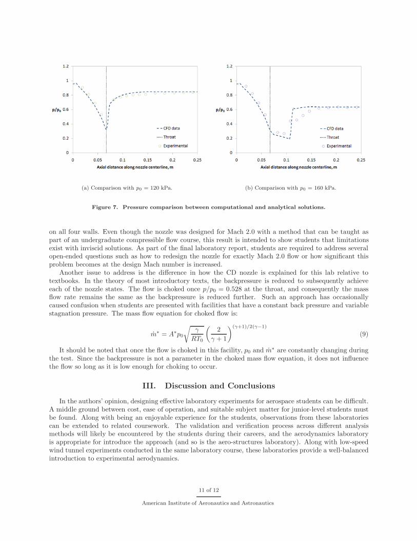
Figure 8 shows comparisons between experimental, computational, and analytical methods for the Machnumber and pressure distributions in the nozzle. The one-dimensional analytical solution has the lowestpressure ratio and highest Mach number in the constant area section because viscous effects are completelyneglected. The two-dimensional numerical solution contains boundary layers on the wall, which effectivelyreduces the area ratio of the nozzle and causes the average Mach number to drop to about 1.95. The three-dimensional experimental Mach number drops even further (about Mach 1.85) due to the boundary layers

9 of 12


Figure 6. Schlieren photographs of different nozzle states.

10 of 12


(a) Comparison with p0 = 120 kPa. (b) Comparison with p0 = 160 kPa.

Figure 7. Pressure comparison between computational and analytical solutions.

on all four walls. Even though the nozzle was designed for Mach 2.0 with a method that can be taught aspart of an undergraduate compressible flow course, this result is intended to show students that limitationsexist with inviscid solutions. As part of the final laboratory report, students are required to address severalopen-ended questions such as how to redesign the nozzle for exactly Mach 2.0 flow or how significant thisproblem becomes at the design Mach number is increased.

Another issue to address is the difference in how the CD nozzle is explained for this lab relative totextbooks. In the theory of most introductory texts, the backpressure is reduced to subsequently achieveeach of the nozzle states. The flow is choked once p/p0 = 0.528 at the throat, and consequently the massflow rate remains the same as the backpressure is reduced further. Such an approach has occasionallycaused confusion when students are presented with facilities that have a constant back pressure and variablestagnation pressure. The mass flow equation for choked flow is:

m∗ = A∗p0

√γ

RT0

(2

γ + 1

)(γ+1)/2(γ−1)

(9)

It should be noted that once the flow is choked in this facility, p0 and m∗ are constantly changing duringthe test. Since the backpressure is not a parameter in the choked mass flow equation, it does not influencethe flow so long as it is low enough for choking to occur.

III. Discussion and Conclusions

In the authors’ opinion, designing effective laboratory experiments for aerospace students can be difficult.A middle ground between cost, ease of operation, and suitable subject matter for junior-level students mustbe found. Along with being an enjoyable experience for the students, observations from these laboratoriescan be extended to related coursework. The validation and verification process across different analysismethods will likely be encountered by the students during their careers, and the aerodynamics laboratoryis appropriate for introduce the approach (and so is the aero-structures laboratory). Along with low-speedwind tunnel experiments conducted in the same laboratory course, these laboratories provide a well-balancedintroduction to experimental aerodynamics.

11 of 12


(a) p/p0. (b) Mach number.

Figure 8. Pressure ratio and Mach number comparison between experimental, computational, and analyticalmethods for perfectly expanded flow.

Acknowledgments

The authors gratefully acknowledge funding for the laboratory development from the University Library,Equipment, Repair and Rehabilitation fund. The authors thank Professor Erian Armanios, Chair of theMechanical and Aerospace Engineering Department, and Professor Bill Carroll, Dean of the College ofEngineering, for their support. The authors would like to thank Satoshi Ukai who designed the free jetexperiment and to Rod Duke who helped to install the hardware.

References

1Pierce A.J. and Lu, F.K., “Laser alignment method for portable schlieren system,” 39th AIAA Fluid Dynamics Confer-ence, AIAA Paper 2009–3574, June 22–25, 2009, San Antonio, Texas.

2Pope A. and Goin, K.L., High-Speed Wind Tunnel Testing, Wiley, New York, 1965.3Tannehill, J.C., Anderson, D.A. and Pletcher, R.H., Computational Fluid Mechanics and Heat Transfer, Taylor & Francis,

Philadelphia, 1997.4Shapiro, A.H., The Dynamics and Thermodynamics of Compressible Fluid Flow, The Ronald Press Company, New York,

1953.

12 of 12


a modern compressible flow laboratory experience for ...arc.uta.edu/publications/cp_files/aiaa...

Documents