A Modelled Visual Multi-Paradigm Modelling andEnactment Environment for Workflow Modelling

Author:Addis GEBREMICHAEL

Promotor:Prof. Dr. Hans VANGHELUWE

MASTER’S THESIS

A thesis submitted in fulfillment of the requirementsfor the degree of Master of Science: Computer Science

in theModelling, Simulation and Design Lab

Department of Mathematics and Computer Science

August 25, 2017

Abstract

In multi-paradigm modelling, workflow (process) modelling is used to precisely describe the order of execution of model oper-ations applied on a set of formalisms. The UML 2.0 Activity Diagrams, used in this thesis, inherently possess design patternsfor modelling concurrency and synchronization, among others, at a high level of abstraction. In addition, activities in a processmodel (PM) can orchestrate with external services. Such behaviours of workflow modelling require that they should be explicitlymodelled. This thesis, thereby, realizes the semantics of a PM using Statecharts Class-diagram (SCCD) formalism. SCCD fa-cilitates the specification of dynamic-structure systems that are timed, autonomous and reactive. Moreover, SCCD is a low-levellanguage where its semantic domain is already defined and simulated. Denotationally mapping PM onto SCCD, thus, providedexplicit modelling of its behaviour such as concurrency, and essentially enabled the enactment of the PM itself. Furthermore,expressing the behaviour of PM activities in an explicitly modelled SCCD allowed interactivity of a PM with an external serviceand/or a user. A visual modelling environment that integrates the graphical concrete syntax of both languages (PM and SCCD) isdeveloped using Tkinter on top of the Modelverse, which is a multi-paradigm modelling and simulation environment. The userinterface behaviour of the visual editor is also explicitly modelled in SCCD.

1

Acknowledgments

I would like give many thanks to Prof. Vangheluwe for introducing me to the state of the art in the field of software engineering.I am also very grateful for the MSDL associates for constantly assisting me throughout this research.Lastly, i would like to thank God, my mother, close family and friends, without whom i would not have managed to come anyfar.

2

Contents

1 Introduction 71.1 Context . . . . . . . . . . . . . . . . . . . . . . . . . . . . . . . . . . . . . . . . . . . . . . . . . . . . . . . . 71.2 Problem statement . . . . . . . . . . . . . . . . . . . . . . . . . . . . . . . . . . . . . . . . . . . . . . . . . . 71.3 Expected contributions . . . . . . . . . . . . . . . . . . . . . . . . . . . . . . . . . . . . . . . . . . . . . . . . 81.4 Outline . . . . . . . . . . . . . . . . . . . . . . . . . . . . . . . . . . . . . . . . . . . . . . . . . . . . . . . . 8

2 Background 92.1 Domain Specific Modelling Languages (DSMLs) . . . . . . . . . . . . . . . . . . . . . . . . . . . . . . . . . . 92.2 Model Operations . . . . . . . . . . . . . . . . . . . . . . . . . . . . . . . . . . . . . . . . . . . . . . . . . . . 102.3 The FTG+PM Language . . . . . . . . . . . . . . . . . . . . . . . . . . . . . . . . . . . . . . . . . . . . . . . 112.4 Statecharts Class-diagram (SCCD) . . . . . . . . . . . . . . . . . . . . . . . . . . . . . . . . . . . . . . . . . . 132.5 Petri-nets . . . . . . . . . . . . . . . . . . . . . . . . . . . . . . . . . . . . . . . . . . . . . . . . . . . . . . . 18

3 Mapping PM onto SCCD 203.1 Mapping Approaches . . . . . . . . . . . . . . . . . . . . . . . . . . . . . . . . . . . . . . . . . . . . . . . . . 203.2 Data Management . . . . . . . . . . . . . . . . . . . . . . . . . . . . . . . . . . . . . . . . . . . . . . . . . . . 263.3 Implementation . . . . . . . . . . . . . . . . . . . . . . . . . . . . . . . . . . . . . . . . . . . . . . . . . . . . 26

4 Visual Editor 344.1 Design Choices and Application Architecture . . . . . . . . . . . . . . . . . . . . . . . . . . . . . . . . . . . . 344.2 Process Model Editor . . . . . . . . . . . . . . . . . . . . . . . . . . . . . . . . . . . . . . . . . . . . . . . . . 364.3 SCCD Editor . . . . . . . . . . . . . . . . . . . . . . . . . . . . . . . . . . . . . . . . . . . . . . . . . . . . . 37

5 Example 405.1 Case Study . . . . . . . . . . . . . . . . . . . . . . . . . . . . . . . . . . . . . . . . . . . . . . . . . . . . . . 415.2 External Service Interaction . . . . . . . . . . . . . . . . . . . . . . . . . . . . . . . . . . . . . . . . . . . . . 43

6 Conclusion 466.1 Future Works . . . . . . . . . . . . . . . . . . . . . . . . . . . . . . . . . . . . . . . . . . . . . . . . . . . . . 46

3

List of Figures

2.1 Graphical concrete syntax of a textual model represented by ”a+b=c” . . . . . . . . . . . . . . . . . . . . . . . . 92.2 An example of a Petri-net model transformation rule . . . . . . . . . . . . . . . . . . . . . . . . . . . . . . . . 102.3 Graphical concrete syntax of ruleBlocks in MoTifs language . . . . . . . . . . . . . . . . . . . . . . . . . . . . 112.4 FTG+PM for the development and verification of a power window case study, adopted from [23] . . . . . . . . . 122.5 A small portion of the UML 2.0 Activity Diagram meta-model . . . . . . . . . . . . . . . . . . . . . . . . . . . 132.6 A subset of UML 2.0 Activity Diagram modelling constructs . . . . . . . . . . . . . . . . . . . . . . . . . . . . 132.7 Two basic states connected by a transition . . . . . . . . . . . . . . . . . . . . . . . . . . . . . . . . . . . . . . 142.8 Composite state B encapsulating two basic states C and D. . . . . . . . . . . . . . . . . . . . . . . . . . . . . . 152.9 Semantics of Statecharts in (a) by ”flattening”. . . . . . . . . . . . . . . . . . . . . . . . . . . . . . . . . . . . . 152.10 Depth/hierarchy in Statecharts. . . . . . . . . . . . . . . . . . . . . . . . . . . . . . . . . . . . . . . . . . . . . 152.11 Parallel state Y with two orthogonal regions A and B . . . . . . . . . . . . . . . . . . . . . . . . . . . . . . . . 152.12 When the transition to the history state is triggered, the state of A will be restored to its last recorded state. . . . . 162.13 This figure illustrates the relation between classes in a Class-diagram and the Statecharts that describe their

behaviour. . . . . . . . . . . . . . . . . . . . . . . . . . . . . . . . . . . . . . . . . . . . . . . . . . . . . . . . 172.14 An enabled transition. . . . . . . . . . . . . . . . . . . . . . . . . . . . . . . . . . . . . . . . . . . . . . . . . . 182.15 A disabled transition. . . . . . . . . . . . . . . . . . . . . . . . . . . . . . . . . . . . . . . . . . . . . . . . . . 182.16 An example of a Petri-net model before (a) and after (b) firing the transition. . . . . . . . . . . . . . . . . . . . . 182.17 A WF-net is a Petri net with a source and a sink place. The goal is that a process initiated via place source

successfully completes by putting a token in place sink [17]. . . . . . . . . . . . . . . . . . . . . . . . . . . . . 19

3.1 Workflow modelling at different levels of abstraction . . . . . . . . . . . . . . . . . . . . . . . . . . . . . . . . 203.2 A simple PM instance expressed using a subset of UML 2.0 ADs constructs . . . . . . . . . . . . . . . . . . . . 213.3 Sequential mapping of PM in figure 3.2 onto the Orchestrator SCCD . . . . . . . . . . . . . . . . . . . . . . . . 223.4 Interleaving branches in parallel regions . . . . . . . . . . . . . . . . . . . . . . . . . . . . . . . . . . . . . . . 233.5 A branch exiting parallel region without synchronizing . . . . . . . . . . . . . . . . . . . . . . . . . . . . . . . 233.6 Process model instances with complex behaviour . . . . . . . . . . . . . . . . . . . . . . . . . . . . . . . . . . 233.7 The Orchestrator SCCD using generic mapping . . . . . . . . . . . . . . . . . . . . . . . . . . . . . . . . . . . 243.8 Orthogonal components of the Orchestrator parallel state in figure 3.7, mapping an Executable, Fork and a Join

node . . . . . . . . . . . . . . . . . . . . . . . . . . . . . . . . . . . . . . . . . . . . . . . . . . . . . . . . . . 253.9 Orthogonal components of the Orchestrator parallel state in figure 3.7, mapping a Start, Decision and a Finish

nodes . . . . . . . . . . . . . . . . . . . . . . . . . . . . . . . . . . . . . . . . . . . . . . . . . . . . . . . . . 253.10 Data-flow representation at design-time using UML 2.0 Activity Diagram constructs . . . . . . . . . . . . . . . 263.11 Process Model abstract sytanx expressed in Class-diagram meta-language . . . . . . . . . . . . . . . . . . . . . 273.12 Process Model graphical concrete syntax adopted by the developed editor . . . . . . . . . . . . . . . . . . . . . 273.13 Statecharts abstract syntax expressed in Class-diagram meta-language. . . . . . . . . . . . . . . . . . . . . . . . 283.14 SCCD graphical concrete syntax adopted by the developed editor . . . . . . . . . . . . . . . . . . . . . . . . . . 283.15 Model transformation which creates the Orchestrator SCCD enclosed in an Atomic rule-block . . . . . . . . . . 303.16 ’ModifyForkToFork’ rule . . . . . . . . . . . . . . . . . . . . . . . . . . . . . . . . . . . . . . . . . . . . . . 303.17 ’RemoveForkToFork’ rule . . . . . . . . . . . . . . . . . . . . . . . . . . . . . . . . . . . . . . . . . . . . . . 30

4

3.18 Model transformation rule in (a) enclosed in Atomic rule-block and (b) in ForAll rule-block . . . . . . . . . . . . 303.19 Model transformation rule enclosed in a ForAll rule-block for mapping an Executable activity to an orthogonal

component in the Orchestrator SCCD parallel state. . . . . . . . . . . . . . . . . . . . . . . . . . . . . . . . . . 313.20 Model transformation rule enclosed in ForAll rule-block used for mapping Fork to an orthogonal component in

the Orchestrator SCCD parallel state . . . . . . . . . . . . . . . . . . . . . . . . . . . . . . . . . . . . . . . . . 323.21 Model transformation rule enclosed in ForAll rule-block used for mapping Join node to an orthogonal component

in the Orchestrator SCCD parallel state . . . . . . . . . . . . . . . . . . . . . . . . . . . . . . . . . . . . . . . . 33

4.1 An overview of the implemented application architecture. . . . . . . . . . . . . . . . . . . . . . . . . . . . . . . 344.2 The developed visual editor for PM. . . . . . . . . . . . . . . . . . . . . . . . . . . . . . . . . . . . . . . . . . 364.3 Prompting user for selecting association types defined in the abstract syntax of PM . . . . . . . . . . . . . . . . 374.4 SCCD visual editor for Activity A in figure 4.2 . . . . . . . . . . . . . . . . . . . . . . . . . . . . . . . . . . . 384.5 State attributes editor in SCCD . . . . . . . . . . . . . . . . . . . . . . . . . . . . . . . . . . . . . . . . . . . . 394.6 Multiple angle points of an edge used for editing its position . . . . . . . . . . . . . . . . . . . . . . . . . . . . 39

5.1 A process model developed in the visual editor for the power window case study. . . . . . . . . . . . . . . . . . 405.2 The executable SCCD model generated after mapping PM to the Orchestrator SCCD . . . . . . . . . . . . . . . 425.3 The behaviour of Combine activity in figure 5.1 modelled in SCCD . . . . . . . . . . . . . . . . . . . . . . . . 435.4 EBNF grammars of LoLA’s file format. . . . . . . . . . . . . . . . . . . . . . . . . . . . . . . . . . . . . . . . 445.5 SCCD model in the developed visual editor which depicts the behaviour of an external service interaction. . . . . 45

5

Listings

3.1 Schedule of model transformation rules used for mapping PM to SCCD . . . . . . . . . . . . . . . . . . . . . . 293.2 Model transformation rule in the Modelverse . . . . . . . . . . . . . . . . . . . . . . . . . . . . . . . . . . . . 324.1 SCCD instance of a Button type used for developing the visual editor expressed in SCCDXML notation . . . . . 35

6

1Introduction

This chapter presents an introduction to the context of this thesis and the problems it addresses.

1.1 Context

Modeling takes a prominent role in the development phase of complex and software-intensive systems. In Model-driven Engi-neering (MDE), Multi-Paradigm Modelling (MPM) advocates to use the most appropriate formalism(s) to explicitly model allrelevant aspects of a system including the process, at the right level of abstraction [5]. Hence, inherent to the nature of MPM is theuse of a wide range of appropriate formalisms, i.e. Domain Specific Modelling Languages (DSMLs), and associated operationsused to manipulate the formalisms. These two aspects can be ideally integrated in the Formalism Transformation Graph and Pro-cess Model (FTG+PM) framework [9]. FTG lays down the relationships among the multitude of DSMLs and model operationsused for the development of a particular system(s) in a given domain. A Process Model is used in conjunction with the FTG tomodel the order of execution of model operations applied on a set of formalisms, and ultimately for a particular motive. In thatregard, a process model captures and exhaustively describes the control-flow and data-flow of the process MPM is being appliedto, which can be used not merely for documentation purposes but also for its enactment, analysis and optimization. The PM usedin this thesis is a subset of the Unified Modelling Language (UML) 2.0 Activity Diagrams, where the UML is a standard in theMDE community [11]. The Modelverse is a prototype tool with the support for all aspects of MPM including the integration andenactment of FTG+PM [23].

1.2 Problem statement

Process models have design patterns for modelling concurrency and synchronization behaviour, among others, at a high-levelof abstraction. In the enactment of FTG+PM in the Modelverse, such behaviours of PM are not explicitly modelled. Althoughcontrol-flow behaves according to the language constructs, activities in a parallel region, for instance, have sequential executionwhich deviates from its actual semantics.PM activities can also coordinate with external services. While requesting for a given service, the PM shall autonomously handleits behaviour, such as lack of service response and/or connection timeouts. This requires explicit modelling of its behaviour withthe support for timed events, triggering of events and handling them autonomously, and reacting to external events.Hence, this thesis aims to assess how it can be possible to model workflows (processes) at different levels of abstraction, such thatit enables to explicitly model its control-flow behaviour and essentially enact the PM itself. In addition, this thesis explores howwe can explicitly model the behaviour of PM activities that interact with an external service and/or a user. In support of modellingat multiple levels of abstraction (of PM with a low-level language), an integrated visual modelling environment is desired. Todeal with the inherent complexities of user interface interaction behaviour, the visual editor is to be explicitly modelled with anappropriate formalism.

7

1.3 Expected contributions

The principal objective of this thesis is to assess and demonstrate how it can be possible to define the semantics of PM in alow-level language, such that control-flow and activities of PM can be explicitly modelled and essentially enacted. In that regard,this thesis uses Statecharts Class-diagram (SCCD) as the appropriate low-level language where its semantic domain is alreadydefined and simulated. SCCD is a hybrid formalism which combines the object-oriented expressiveness of Class-diagramswith the behavioural discrete-event characteristics of Statecharts. This, in turn, facilitates the specification of dynamic-structuresystems that are timed, autonomous and reactive.Upon successful completion of this thesis, we will discuss how we can denotationally map PM onto SCCD, and demonstratethe enactment of PM in which its semantics is given in SCCD. Moreover, by encapsulating the behaviour of PM activities in anexplicitly modelled SCCD, we will show how the PM autonomously behaves while interacting with an external service and/or auser. The graphical concrete syntax of both languages can be used to develop an integrated visual modelling environment whereit can be possible to model workflows at different levels of abstractions. The visual editor, to be developed in Tkinter, is supposeto interact with the Modelverse as a model repository, and in support of a multi-paradigm modelling and simulation environment.The user interface of the editor is to be explicitly modelled in SCCD, as it entails a behaviour that is timed, autonomous, reactiveand has a dynamic-structure.

1.4 Outline

The remainder of this thesis is structured in the following manner. The next chapter gives a background introduction on the threemain aspects of MPM, i.e. language engineering (DSMLs), model operations, and process modelling. In addition, it also givesa concise introduction to the SCCD formalism and Petri-nets. Chapter 3 has an extended discussion on the approaches exploredand the implementation of mapping PM onto SCCD. Chapter 4 explains the design choices made and the implementation of thedeveloped integrated visual editor. Chapter 5 has a case study as an example for demonstrating the semantics of PM given inSCCD, and elaborates the behaviour of an external service and/or a user interaction of PM activity, which is explicitly modelledin SCCD. The external service is an optimal reachability analysis of a Petri-net model available outside of the FTG. Finally,chapter 6 concludes this thesis by summarizing the research and reflecting on our findings, followed by future works that canfurther be incorporated as part of this research.

8

2Background

This chapter gives an introduction to model-driven engineering concepts and techniques in which the research in this thesisfinds relevant. It starts by explaining the core concepts behind MPM, that includes domain-specific modelling languages, modeloperations and process modelling. It also highlights the support of these three aspects of MPM by a prototype tool used in thisresearch, i.e. the Modelverse [23]. Following is a concise introduction to the SCCD formalism and Petri-nets. While discussingPetri-nets, this chapter also introduces to the idea of workflow-nets. Workflow-nets are a particular class of Petri-nets that havebecome one of the standard ways to model and analyze workflows [17].

2.1 Domain Specific Modelling Languages (DSMLs)

Model-driven engineering (MDE) is currently the mainstream approach to the development of complex and software-intensivesystems. Its underlying philosophy starts by developing domain-specific structural and behavioral models of the system underdevelopment [9]. Domain-specific means that initially models of the system should be described in a language close to thedomain being addressed. This essentially reduces the accidental complexity of a software engineering process by shifting thespecification from computing concepts to conceptual models or abstractions with in the problem domain. Hence, DSMLs aremore user intuitive, easy to learn, and maximally constrain the user, allowing to reduce errors. Models created in DSMLs areused for documentation, analysis, simulation and code generation for multiple platforms [20].A DSML can be fully defined by [8]:

• Its abstract syntax, defining the DSML constructs and their allowed combinations. This information is typically capturedin a meta-model, where the DSML being developed conforms to.• Its concrete syntax, specifying the visual representation of the different constructs. This representation can be either

graphical (using icons), or textual.• Its semantics, defining the meaning of models created in the domain. This encompasses both the semantic domain (what

is its meaning) and the semantic mapping (how to give it meaning).

Figure 2.1: Graphical concrete syntax of a textual model represented by ”a+b=c”

This can be more elaborated with a trivial, and simple to understand, example as follows. Figure 2.1 and the string of characters”a+b=c” can both be seen as an equivalent visual representation of the same model, graphically and textually respectively. Thisvisual representation of the model is for the abstract syntax concept of an operation (addition) that takes in signal ’a’ and signal’b’, followed by another operation (assignment) which produces signal ’c’. The abstract syntax is a representation in memory

9

with some kind of data structure for the variables and operations used in this model. Nonetheless, the semantics or ”meaning” ofthe model is yet to be defined in the semantic domain, which, if assumed to be, is the set of real numbers (i.e. what the variablesevaluates to), with the semantic mapping being the computation (algorithmic simulation) of the operations (i.e. how the variablesare evaluated).The Modelverse allows for language engineering through meta-modelling, where languages are themselves instances of the meta-language and can thus be seen as models themselves [23]. This offers users a multitude of possibilities to create new DSMLswithout modifying the tool. The Modelverse is also a model repository in a sense that it runs as a service and enables users toshare models and languages.

2.2 Model Operations

Another aspect of MPM is model operations. Model operations are used to manipulate models for some use. It can be for definingthe semantics of a modelling language or can simply be for model management operations such as model merge and split, whichis irrespective of their semantics. Model operations define the semantics of a model instance denotationally (by mapping ontoanother language where its semantic is already defined) or operationally (by directly executing the model producing executiontrace or simulation) [23]. The core of this thesis research is to define the semantic domain of a process model denotationally, bymapping it onto SCCD, where SCCD has an existing semantics and is executable.Model operations are commonly expressed using either action language code or model transformations. This thesis research usesmodel transformations, which are based on the work in the graph transformation community [12]. In this context, transformationrules consists of the smallest units in which a change from source model to target model can be defined. Rules use patterns andgraph rewriting algorithms to ultimately define CRUD operations on a model. Patterns can be of two types, pre-condition andpost-condition. Pre-condition patterns have a read-only operation and are used to determine when and which elements of thesource model are to be transformed. While a post-condition has a create, update and delete operation and determines how thesource model can be transformed. Model transformations are models in themselves and can be visualized as in figure 2.2. This

Figure 2.2: An example of a Petri-net model transformation rule

representation depicts three patterns out of which the first two are pre-condition patterns and the last a post-condition. The patternin the left hand side (LHS) contains all the positive reads while the pattern in the negative application condition (NAC) holds thenegative reads of this rule. Both patterns help in determining the pattern to be found. When found, the pattern is replaced by theright hand side (RHS), which represents the result after the rewriting phase. The elements to be deleted are elements that have apositive read, and thus appear in the LHS, but do not appear in the RHS. Likewise, elements that are added appear in the RHS,but not in the LHS. In the example on figure 2.2, a petri-net model with a place (labelled 0) and a transition (labelled 1) pattern issearched for in the LHS. If the pattern is found given the NAC is not satisfied, i.e. an arc is not created for that pattern, it updatesthe model in the RHS by adding an arc (labelled 2).After having defined the rules, the next step is scheduling of the defined rules for execution. To illustrate how the scheduling ofrules works, the MoTifs [15] , a model transformation language, is used. Before having to discuss further on how the schedulingworks, MoTifs uses the concept of RuleBlocks to encapsulate the rules. The reason for encapsulating rules in these RuleBlocksand the scheduling of them is mainly because a rule in itself does not specify weather CRUD operations should be applied onhow many of the matches found in the model and in what order multiple rules shall execute. Figure 2.3, depicts the concretesyntax of the MoTifs language available constructs, and their description is discussed as follows.

• ARule: Atomic rule executes the rule for one match found. If no matches are found, it fails.• QRule: A query rule succeeds if the LHS matches and the NACs do not match. The RHS of the rule is ignored.• FRule: For-all rule executes the rule for each match in the match set. It fails if no matches can be found.• SRule: Sequence rule executes the rule until no more matches can be found. It fails if no matches can be found.

10

• BRule: Allows for other rule-blocks to be nested and executes ,non-deterministically, one of the succeeding child rule-blocks.• CRule: Allows nested transformation. The referenced transformation schedule is executed once.• BSRule: Also allows for defining hierarchy by nesting other rule-blocks and executes (non-deterministically) one of the

succeeding child rule-blocks until none of them succeeds.• PRule: Allows for different ruleBlocks to be executed in parallel.• LRule: Defines loops and its condition using an atomic rule-block. The body of the loop has a CRule rule-Block. As long

as the atomic rule-block succeeds, a CRule will be executed.

Figure 2.3: Graphical concrete syntax of ruleBlocks in MoTifs language

Each ruleBlock has a public interface with an input port, represented by a triangle, and two output ports, where 3 representssuccess and 7 for failure.Similar to creating models in the Modelverse, this tool also enables the creation of model operations as models themselves,allowing several language instances to be executed. Thus, adding or modifying model operations does not alter the tool itself.There are some tools that use imperative languages, such as metadepth [2] which uses EOL, others like AToMPM [16] use modeltransformations. The Modelverse has support for both, model transformations through RAMification and explicitly modelledaction language. Model transformation through RAMification is often used with MPM [23]. RAMification is the process ofmodifying the meta-model of a language in such a way that it can be used in the patterns of transformation rules. With thisapproach, the model operations including source and target languages are all explicitly modelled.

2.3 The FTG+PM Language

The last aspect of MPM is process modelling. A Process Model (PM) is used in combination with the Formalism TransformationGraph (FTG), constituting the two sub-languages of the FTG+PM framework. With a wide range of formalisms and modeloperations utilized in the application of MPM, it can get quite confusing and difficult to execute model operations in a reproduciblemanner. Hence, the FTG+PM language provides a complete approach by offering an overview of all foramalisms and theirrelations, i.e. the operations between them. In addition, it manages the various modelling artifacts created and the process itself.As this section gives a brief introduction to FTG+PM, further detail of this framework can be found in [9].The FTG presents all used formalisms (DSMLs) and their relations (model operations) to be used in a process. It is representedby a hypergraph with languages as nodes and transformations as edges. It formulates the relationships among the various domain-specific languages and transformations used for the development of a particular system(s) in a certain domain. As depicted infigure 2.4, languages in the FTG are denoted by labelled rectangles, and transformation operations denoted by labelled circles onthe edges. The incoming edges towards an operation show the source languages of the transformation while the outgoing edgesfrom an operation point to the target languages. It can also be the case where the FTG model may include self directed loops,given the source and target languages remain the same.

A PM manages the used formalisms and their relations for a particular intent and can be used for documentation, enactment(i.e. automatic execution and chaining of operations), analysis and optimization. A PM generally consists of two types of nodes,namely operations and data. Operations are commonly model transformations, which is an automatic procedure, but can also be

11

Figure 2.4: FTG+PM for the development and verification of a power window case study, adopted from [23]

manual operation where domain experts are required to handle. This can be seen on figure 2.4 where operations/activities are ingrey colour, whereas in yellow are automatic model transformations. Data are the models these operations consume and produce.Thus, operation and data nodes form the two flows, i.e. control-flow and data-flow respectively. Control-flow begins from anorigin point (the Start node) and is followed throughout until the process ends (the Finish node is reached). When control-flowencounters an operation, it executes it. During execution, an operation may consume data. After execution, the operation mayalso produce data and control-flow passes onto the next operation. Thus, data-flow specifies which model(s) are to be used bywhat operation and manages the modelling artifacts created during the process. While control-flow mandates which operationsmust execute in what order and is completely ignorant of what model(s) an operation acts on.The PM in this thesis (taken as a subset of the UML 2.0 Activity Diagrams [14]) may include other operations which specify the

structural (i.e. compositional hierarchy) and behavioural aspects of a process, such as a Fork, Join, and a Decision node. A Forknode represents concurrent execution of activities and influences control-flow in such a way that when control-flow encountersit, all subsequent operations automatically start execution. A Join node synchronizes activities executing in parallel. That meanswhen control-flow encounters a join node, all previously executing activities have finished. A Decision node also influences thecontrol-flow of a process by evaluating its input data with conditional data in its outgoing edges and decides in which of theoutgoing edges control-flow proceeds. A subset of the UML 2.0 Activity Diagrams modelling constructs are shown in figure 2.6and a portion of its meta-model expressed in Class-diagrams in figure 2.5.

Figure 2.4, shows an overview of a FTG+PM model for an automotive domain which describes all the modelling artifactsused, and the process for the intention of building a software system that controls the power window of an automobile. In thecontext of MPM, this case study is often used as it is simple to understand and addresses many of the challenges faced [3][9].At the left hand side, the FTG is shown which presents the different DSMLs used, such as Control, Environment, EncapsulatedPetri-net etc., and all operations among them, such as Control2EPN, Combine, Analyze. In the PM shown on the right hand sideof figure 2.4, we can see that the PM refers to the languages and operations defined in the FTG and presents the order in whichthese operations can be defined. It also captures the specific modelling artifacts (DSMLs) that are propagated among differentoperations, shown in semi-transparent rectangular boxes. The details of the DSMLs and model operations used in this case studyare further discussed in the literature [23][3][9].The PM has a flow that begins with the input of requirements from different domains. Although different requirement can beused, we will focus on the verification aspect of the power window, i.e. we want to substantiate that the power window willnever go up when an object is inserted through. In that regard, Control model is responsible for translating the key-presses (i.e.the Environment model which can be in Up, Down, or Neutral mode) into commands to the engine responsible for window

12

Figure 2.5: A small portion of the UML 2.0 Activity Diagram meta-model

Figure 2.6: A subset of UML 2.0 Activity Diagram modelling constructs

movement. Similarly, domain experts create models for the Plant, Architecture and a safety query in a domain-specific language.The Control2EPN operation is, for instance, a model transformation which takes in, as data input, an instance of a Control modeland produce an Encapsulated Petri-net (EPN). Similarly, Plan, Environment, Architecture are transformed to an EPN model andare combined by the Combine operation which yields a marked Petri-net. This Petri-net is then used to conduct a reachabilityanalysis and, thus, produces a reachability graph. Note the use of a safety-query, also given as a model, which specifies a placep with a single token in it. Ultimately, if the query is found in the reachability graph by the Mark operation, it is deemed unsafeand control-flow goes back to a point where all domain experts revise their models, given as a manual operation. Otherwise, thesystem is deemed safe, and the process terminates.The Modelverse has full support for the use of process models including their enactment, i.e. chaining of automatic operations.With the repository nature of the Modelverse, coupled with the processes themselves being models, it is possible for processes tobe shared among different users with permission access. Sharing the FTG+PM, thereby, allows users for reproducability by onlyenacting the same PM. Combined with the previously discussed aspects of MPM, the Modelverse offers a fully-fledged supportof the FTG+PM framework, including the enactment of the FTG+PM in this power window case study. This case study is laterused in this thesis to demonstrate the semantic of the PM given in SCCD, and it is further discussed in chapter 5.

2.4 Statecharts Class-diagram (SCCD)

Statecharts, first introduced by David Harel [6], is a visual modeling language that is a higraph-based extension of standardstate-transition diagrams that is used to aid the specification of complex, reactive, timed, autonomous, interactive discrete-eventsystems. It is appropriate for describing large and reactive systems as it naturally adds the notion of depth, orthogonality andmodularity, to ’normal’ Finite State Automata (FSAs) [7]. However it lacks the facilities for specifying the structure of a systemin addition to creating, deleting and communicating multiple Statecharts instances at run-time.Class-diagram, in the Unified Modeling Language (UML) [11], is a visual modeling language that describes the structure of asystem by showing the system’s classes, their attributes, operations (or methods), and the relationships among classes. SCCD

13

[19] is a hybrid formalism which combines the structural object-oriented expressiveness of Class-diagrams with the behaviouraldiscrete-event characteristics of Statecharts. This, in turn, facilitates the specification of dynamic-structure systems that are timed,autonomous and reactive. Classes model both structure and behaviour-structure in the form of attributes and relations with otherclasses, behaviour in the form of methods, which access and change the values of attributes of the class, and a Statecharts model,which describes the modal behaviour of the class, modelling its control-flow. At run-time, a class can be instantiated, whichcreates an object. Objects are initialized according to the classs constructor, and can be deleted, invoking the classs destructor.After initialization, an object is controlled by its Statecharts through changes in the object’s state caused by triggers like eventsand operation invocation. The relationships modelled between classes are instantiated at run-time in the form of links. Theselinks serve as communication channels, over which objects can send and receive events.

In this chapter the Statecharts and Class-diagram (SCCD) formalism is discussed. Many parts of this section are taken from wherethe formalism is first defined [19] and a documentation for the SCCDXML [18] notation. This notation is a concrete textual syntaxrepresentation, used as a serialization format for an existing SCCD compiler that generates code for multiple platforms. Thevarious available constructs of Statecharts and their semantics are discussed first using a neutral visual representation, followedby a discussion of Class-diagram constructs supported by an example illustrating a combination of both Statecharts and Class-diagram in a single SCCD model. Finally, a brief introduction to how events can be used for communication among instancesin SCCD models is discussed followed by a highlight of the object manager, which is in charge of the management of objects atrun-time.

2.4.1 Constructs

In this section the semantics of the different constructs that make up the formalism are discussed. For readability purposes, theconstructs are categorized as either Statecharts constructs or a concept that encapsulate the Statecharts into a class, and ultimatelyinto a Class-diagram.The constructs of Statecharts formalism discussed in this section are based on a neutral visual representation as proposed inHarel’s definition published in 1987 [6]. Statecharts is a visual modelling language that extends finite state automata with addedhierarchy, parallelism, history and broadcast communication. Harel created the formalism to be able to describe large and reactivesystems, as there was no such method available at the time.

Basic State

The basic state acts as the main building block of a Statecharts and is represented by a rounded rectangle as in figure 2.7, wheretwo basic states are depicted. A basic state, like that of composite and parallel states, represents a mode the system can be in.A state can be entered (which executes an optional block of executable content) and exited (which executes an optional block ofexecutable content) using transitions. A Statecharts consisting solely of basic states has to have exactly one default/initial state,this is represented by an incoming edge with a black-dot as a source, as shown in figure 2.7.

Figure 2.7: Two basic states connected by a transition

Transition

In figure 2.7, the two states are connected by a transition originating from the initial state on the left, with a label of the formevent[guard]/action. This means that, if the current state is A, upon reception of the trigger event e, the Statecharts will transitionfrom state A to state B if and only if the guard condition c is satisfied. This guard condition can reference parameter valuesreceived by the transition which catches the event. Upon firing the transition, an action will be executed which in this case israising an event r and an executable content a. Events in SCCD are strings that are accompanied by a number of parametervalues: the sender is obliged to send the correct number of values, and the receiver declares the parameters when catching theevent. Each parameter has a name, that can be used as a local variable in the action associated with the transition that catches theevent. Thus, transitions are triggered by an event or a timeout, or can be spontaneous. They can optionally specify a condition,an action and raising of an event.

14

Figure 2.8: Composite state B encapsulating two basicstates C and D.

Figure 2.9: Semantics of Statecharts in (a) by ”flattening”.

Figure 2.10: Depth/hierarchy in Statecharts.

Composite State

Composite states add a notion of hierarchy to Statecharts. The composite state is also called the XOR state because when sucha state is active, exactly one of its substates must be active. Each composite state should have exactly one initial substate andtransitions can occur at and between every level of the state hierarchy.To illustrate this we look at the example in Figure 2.8. At initialization time, state A is active. Upon reception of the event H, thecomposite state B will be entered and consequently its initial substate C as well. At this point an event K can bring the Statechartsin the state configuration where B and its substate D are active, while an event J would bring the Statecharts back to its initialconfiguration where state A is active. Figure 2.9 shows the semantics of the Statecharts in figure 2.8 by ”flattening” it. We cansee that both substates C and D have an outgoing transition with event J. Thus, either one of the active substates, i.e. C or D canchange the Statecharts configuration back to state A. Nonetheless, in case of non-determinism, i.e. if both the parent state andone of its substates have a transition leaving it on the same event, Statecharts will handle this by either enabling the transitionassociated with the inner substate or the transition associated to the parent state.As mentioned before, with Statecharts it is possible to define actions and output events, that should be raised on either enteringor exiting a specific state. When multiple layers of hierarchy are traversed on firing a transition, these actions are raised in anintuitive way. The exit actions are raised first, from the deepest level up to, but excluding, the first shared parent between thesource and target states. This is then followed by executing the enter actions in the opposite direction down to the target states.

Parallel State

Besides the XOR composition achieved by a composite state, also AND composition is available in the Statecharts formalism.These are better known as parallel states or orthogonal components and allow for parallelism to be modelled. Upon entering aparallel state, each of the orthogonal regions (substates) will become active.

Figure 2.11: Parallel state Y with two orthogonal regions A and B

15

A parallel state is represented the same way as a composite state, however its substates are depicted by dashed rectangles ex-pressing that they are active at the same time. We see such a state in Figure 2.11 labelled Y. Since this is the default state at thetop level, this will directly be entered upon initialization. Consequently both substates A and B will be entered, which ultimatelyresults in both inner states D and K being active at the same time. When the transition of K to L is triggered by the event X, stateD will still remain active. In addition, an action appearing along a transition in Statecharts is not merely sent to the outside worldas an output. Rather, it can affect the behavior of the Statecharts itself in orthogonal components and it is known as broadcasting.This can be achieved by a simple broadcast mechanism, as in the Statecharts shown in figure 2.11, where if an external event Zoccurs, a transition labelled Z/X in orthogonal component A is taken, the action X of the transition is immediately activated andregarded as a new event, possibly causing further transitions in other components, in this case transition labelled X in orthogonalcomponent B.

History State

A history state, which is depicted by a circle with the label H, adds memory to a component. A history state keeps track of thecurrent configuration when its parent state is exited. If a transition has the history state as a target, the configuration that wassaved is restored. If no configuration was saved yet, the default state is entered instead.

Figure 2.12: When the transition to the history state is triggered, the state of A will be restored to its last recorded state.

This can be illustrated further as in Figure 2.12 where there is a composite state A that has a history state and two sub-states ofwhich K is the default one. If an event X is received after initialization, the composite state will reside in sub-state L (i.e., L isnow active). Upon triggering the transition to state M, which is enabled by the event Y, the current sub-state of A is recorded first.When this is followed by an event Z, the transition to the history state is taken resulting in A being reactivated and thus havingthe saved state restored, where sub-state L is active again. Statecharts offers two types of history. The default shallow type onlysaves one layer of state in a component while the deep type saves all descendants of the component. The latter is represented byadding an ’asterisk’ (*) to the state label resulting in H*.

Classes

The top level of a SCCD model resembles a UML Class-diagram with classes and edges connecting them. Classes are the mainaddition of the SCCD language. They model both structure and behaviour - structure in the form of attributes and relations withother classes, behaviour in the form of methods, which access and change the values of attributes of the class, and a Statechartsmodel, which describes the modal behaviour of the class modelling its control-flow. At run-time, a class can be instantiated, whichcreates an object. Objects are initialized according to the classs constructor, and can be deleted, invoking the classs destructor.After initialization, an object is controlled by its Statecharts through changes in the objects state caused by triggers such as eventsand operation invocations. An SCCD model can also have an external class, denoted by a dotted rectangular box, which can bereferenced from outside and thus can not be linked to a Statecharts for its behavioural specification. The relationships modelledbetween classes are instantiated at run-time in the form of links. They serve as communication channels, over which objects cansend and receive events.

16

Class Relationships

Classes can have relationships with other classes. There are two types of relationships: associations and inheritance. An associ-ation is defined between a source class and a target class, and has a name. It allows instances of the source class to send eventsto instances of the target class by referencing the association name. An association has a multiplicity, which defines the minimaland maximal cardinality. They control how many instances of the target class have to be minimally associated to each instanceof the source class, and how many instances of the target class can be maximally associated to each instance of the source class,respectively. Each time an association is created, it results in a link between the source and target object. This link gets a uniqueidentifier, allowing the source object to reference the target, for example to send events.An inheritance relation results in the source of the relation to inherit all attributes and methods from the target of the relation.Specialisation of modal behaviour (i.e., (parts of) the SCXML model of the superclass) is currently not supported. Inheritanceedges have a priority attribute which allows to specify in which order classes need to be inherited (in case of multiple inheritance).Inheritance relations with higher priority are inherited from first.In Figure 2.13 we can see the Class-diagram from the perspective of a single class, i.e. ClassD. This class is related with classesClassE and ClassF by an inheritance edge and a named unidirectional association edge labelled ’assocation g’, respectively.Finally, a dashed edge with label <<behaviour>> is used to link the class to its corresponding Statecharts.

Figure 2.13: This figure illustrates the relation between classes in a Class-diagram and the Statecharts that describe their be-haviour.

2.4.2 Events in SCCD

In the traditional Statecharts formalism, when casting an event, it was obvious that the scope of an event was local to theStatecharts that generates it. Now SCCD adds the ability to transmit events to class instances and to output ports with theaddition of a public input/output interface using ports, as well as classes and associations. Thus, different levels of scope areadded as described below by the different scope names used in the action associated with a transition that catches an event.

• local: The event will only be visible for the sending instance.• broad: The event is broadcast to all instances.• output: The event is sent to an output port and is only valid in combination with the port attribute, which specifies the name

of the output port.• narrow: The event is narrow-cast to specific instances only, and is only valid in combination with the target attribute, which

specifies the instance to send the event to by referencing a link.• cd: The event is processed by the object manager. See the next section for more details.

2.4.3 Object Manager

At run-time, a central entity called the object manager is responsible for creating, deleting, and starting class instances, as wellas managing links (instances of associations) between class instances. It also checks whether no cardinalities are violated: whenthe user creates an association, it checks that the maximal cardinality is not violated, and when the user deletes an association, itcheck whether the minimal cardinality is not violated. As mentioned previously, instances can send events to the object managerusing the cd scope. The object manager can thus be seen as an ever-present, globally accessible object instance, although it isimplicitly defined in the run-time, instead of as a SCCD class.

17

Figure 2.14: An enabled transition. Figure 2.15: A disabled transition.

Figure 2.16: An example of a Petri-net model before (a) and after (b) firing the transition.

When the application is started, the object manager creates an instance of the default class and starts its associated Statechartsmodel. From then on, instances can send several events such as associate instance and delete instance to the object manager tocontrol the set of currently executing objects.

2.5 Petri-nets

Petri-nets are mathematical models used for describing discrete event dynamic systems [1]. A classical Petri-net is a directedbipartite graph with two node types, namely Places and Transitions. The nodes are connected via directed arcs, of whichconnection between two nodes of the same type is not allowed. Places are represented by circles and transitions by rectangles, asin figure 2.14 which depicts a simple Petri-net model .

Definition 2.5.1. A Petri-net is a 5-tuple (P, T, A, ω,M0) [10], where

• P = {p1,p2,..pn} is set of finite Places• T = {t1,t2,..tn} is set of finite Transitions• A ⊆ (P×T) ∪ (T×P) set of arcs (flow relation)• ω : A→ N a weight function• M0 : P→ N an initial marking

At any time a place in a Petri-net model can contain zero or more tokens, represented by small black dots. The state (marking)of the Petri-net is the distribution of tokens over its places. Given a place (as source) connected to a transition (as target) usingan arc, the place is refereed to as an input place of the transition. Likewise, when a transition (as source) is connected to a place(as target) with an arc, this place is called an output place of the transition. A transition without input place(s) is called a sourcetransition whereas a sink transition has no output place(s).The semantic mapping of a Petri-net model can be simulated in its reachability or coverability graph by using the standard firingrule. A transition t is said to be enabled with respect to some marking M if and only if each input place p of t contains equalto or greater than the weights placed on the arcs connecting p to t. Note that a source transition is always enabled. An enabledtransition t may fire, and if it fires, t consumes as many token(s) as the weights placed on each arc from p to t. In addition,transition t also produces for each p, as many token(s) as the weights places on each arcs from t to output place p. In the examplePetri-net model on figure 2.14, we can see two input places for the transition and that it is enabled. After firing, as depicted onfigure 2.15, it no longer becomes enabled given that there is not at-least one token in place p1.Petri-nets are very intuitive due to their simple graphical concrete syntax. They are commonly used for analysis of complexsystems with shared resources such as distributed systems, parallel programs, control systems, shared memory and networks [1].

2.5.1 Workflow-nets and Soundness Properties

Workflow nets (WF-nets) are a particular class of Petri-nets, used to model and analyze workflow procedures. A worflowprocedure specifies the set of partially ordered tasks required to process workflow cases successfully. Petri-nets which modelworkflow procedures have two typical properties. First, they always have two special places i and o, which correspond to thebeginning and termination of a workflow procedure respectively. Place i is a source place and o is a sink place. Second, foreach transition t and place p, there should be a directed path from place i to o via t and p. A Petri net which satisfies thesetwo requirements is called a Workflow net [17]. Figure 2.17 depicts a workflow-net with a source and a sink place. The”cloud” represents a process which can be initiated by putting token(s) on the input place source and the goal is that the processsuccessfully completes by putting a token in place sink.Having (PN,M) to denote a Petri-net PN with some initial state marking M, let us see some properties of a Petri-net that are usedto derive the soundness properties of a workflow-net.

18

Figure 2.17: A WF-net is a Petri net with a source and a sink place. The goal is that a process initiated via place sourcesuccessfully completes by putting a token in place sink [17].

Definition 2.5.2. (Live) A Petri net (PN,M) is live if for every reachable state M’ and every transition t, there is a state M”reachable from M’ which enables t.

Definition 2.5.3. (Bounded) A Petri net (PN,M) is bounded if for every reachable state and every place p, the amount of tokenis p is bounded.

A workflow-net such as the one depicted in Figure 2.17, is sound if and only if the following three requirements are satisfied:[17]

• Option to complete- For every state M reachable from the initial state i, there exists a firing sequence leading from state Mto a state which just marks the place sink.• Proper completion- When the state which marks the place sink is reached, the state configuration of all other places should

be empty.• No dead transitions - it should be possible to execute an arbitrary activity by following the control-flow of a workflow-net.

Hence, the soundness properties stated above can be translated to the liveness and boundedness problem, i.e. a Workflow-net issound if and only if it is live and bounded.

19

3Mapping PM onto SCCD

As the underlying aspect of this thesis research is to define the semantics of PM in SCCD, this chapter gives an elaborateddiscussion on the approaches explored and an implementation, in the Modelverse, of denotationally mapping PM onto SCCD.

3.1 Mapping Approaches

Apparent to both languages (PM and SCCD) is the use of common design patterns such as hierarchical composition, sequential-execution, concurrency and synchronization, multiple instantiation (of PM activities or SCCD class instances) through sequentialiteration, and the support for data exchange among the modelling constructs. A PM has two nodes , i.e. activity and data, and anedge associating activities. Activities can be of an executable type or a control node such as Fork and Join which influence thecontrol-flow of a process. An executable activity is a model operation or an external service which consumes and/or producesdata as models. The behaviour of such an activity is to be expressed in an explicitly modelled SCCD.While encapsulating SCCD in PM executable activity, the executable corresponds to a single SCCD instance, as depicted on

Figure 3.1: Workflow modelling at different levels of abstraction

figure 3.1. This figure shows a PM with multiple levels of abstraction where the behaviour of PM activities is expressed ina low-level language (SCCD). Hence, model operations and/or external services can be explicitly modelled in the Statechartsbelonging to the Class-diagram instance. Nonetheless, the PM is still the one in charge of managing the creation and executionorder of an executable (expressed in SCCD instance), in addition to controlling the data artifacts produced and consumed. ThePM, thus, needs to be mapped onto a SCCD instance(s), so that ultimately the PM can be realized as one SCCD model, whichcan then be executed.From here on, we will refer to the mapped SCCD instance as the Orchestrator and it entails the two main responsibilities ofPM, i.e. managing the control-flow and data-flow of a process. Managing the control-flow means that the Orchestrator (as the

20

default SCCD) is created first and bears the responsibility of controlling the order of spawning SCCD instances according to thesemantics of PM constructs influencing its control-flow. In addition, the Orchestrator is in charge of organizing the data artifactsin such a way that, while simulated, it should be well aware of which data is consumed and/or produced by which SCCD instancethat is related to an executable.There are two approaches explored in this research that would make the mapping of PM onto SCCD Orchestrator possible. Forsimplicity, we can leave the data-flow aspect to be discussed in the subsequent section. The two approaches with their relatedbenefits and limitations are discussed next.

3.1.1 Sequential Mapping

In sequential mapping, PM constructs are mapped onto SCCD constructs in a more intuitive way by fully exploiting the commondesign patterns inherent to both languages. This can be illustrated in the following example. Figure 3.2, depicts a simple PMinstance consisting of a subset of the UML 2.0 ADs constructs. A denotational mapping of the PM in figure 3.2 is shown in thecorresponding Orchestrator Statecharts in figure 3.3.

At initialization time of the Orchestrator SCCD instance, the initial state is entered, i.e. the parallel state with orthogonal

Figure 3.2: A simple PM instance expressed using a subset of UML 2.0 ADs constructs

components. This is related to the PM where at the start, control-flow encounters a Fork node, denoting concurrent executionof activities A and B. Similarly, when the parallel state is entered in the Orchestrator Statecharts, it will have all its orthogo-nal components active. The behaviour of SCCD instances related to an executable activity can be described with three basicstates as children of a hierarchical state, such as the orthogonal component ’activity A’ or the composite state ’activity C’ infigure 3.3. When each orthogonal component in the parallel state is entered, the initial states become active, and raise a ’cre-ate instance’ event to the object manager of SCCD, responsible for creating the corresponding SCCD instance. Upon receiving’instance created’ event back from the object manager (by the event attached to the transition originating from the initial state),the orthogonal component transitions to a running state and waits until it receives a ’terminated’ event from its correspondingSCCD instance. When that happens, the orthogonal component transitions to a finish state, where it raises a local event ’finished’.

21

Figure 3.3: Sequential mapping of PM in figure 3.2 onto the Orchestrator SCCD

The third orthogonal component is a mapping of the Join construct in the PM. This orthogonal component’s initial waiting statealso becomes active when the parallel state is entered. Attached to this state is a transition that listens to the ’finished’ event raisedby the rest of the orthogonal components. Every time this transition triggers, it takes an action which removes the element whoraised the ’finished’ event from its collection. While mapping, this collection can be initialized with names of activity nodes theJoin synchronizes from the PM. The other transition, targeting the synchronized state, will be triggered when the guard conditionbecomes valid, i.e. the collection becomes empty. At this point, all orthogonal components have reached their ’finish’ state,thereby synchronized. The synchronized state of the Join orthogonal component is also entered and raises a ’synch’ event whichtriggers the transition exiting the parallel state. This denotes the synchronization of activities A and B by a Join node in thecorresponding PM in figure 3.2.In a similar manner, the state transitioning (flow of control) continues until the ’decision’ state, mapped to Decision node in thePM, is reached. This time, the conditions placed upon the state will be evaluated to direct the flow of control. The evaluationcompares the data consumed by the Decision at run-time, with data values placed on the outgoing edges of the Decision nodein the corresponding PM. This data from the PM can be supplied to the mapped ’decision’ state in the Orchestrator during themapping (model transformation) process. Hence, in this model, if the evaluation results to be False, the process will reach an’end’ state. Otherwise, it will transition back to the parallel state, where all orthogonal components enter their initial states. This,thereby, enables for sequential multiple instantiation of the SCCD instances.

22

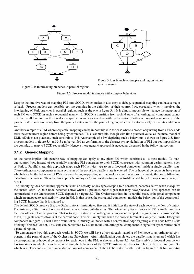
Figure 3.4: Interleaving branches in parallel regions

Figure 3.5: A branch exiting parallel region withoutsynchronizing

Figure 3.6: Process model instances with complex behaviour

Despite the intuitive way of mapping PM onto SCCD, which makes it also easy to debug, sequential mapping can have a majorsetback. Process models can possibly get too complex in the definition of their control-flow, especially when it involves theinterleaving of Fork branches in parallel regions, such as the one in figure 3.4. It is almost impossible to manage the mapping ofsuch PM onto SCCD in such a sequential manner. In SCCD, a transition from a child state of an orthogonal component cannotexit the parallel region, as this breaks encapsulation and can interfere with the behavior of other orthogonal components of theparallel state. Transitions only from the parallel state can exit the parallel region, which will automatically exit all its children aswell.Another example of a PM where sequential mapping can be impossible is in the case where a branch originating from a Fork nodeexits the concurrent region before being synchronized. This is admissible, though with little practical value, as the meta-model ofUML AD does not place any such constraints [14]. An example of a PM depicting such a behaviour is shown on figure 3.5. Bothprocess models in figure 3.4 and 3.5 can be verified as conforming to the abstract syntax definition of PM but yet impossible ortoo complex to map to SCCD sequentially. Hence a more generic approach is needed as discussed in the following section.

3.1.2 Generic Mapping

As the name implies, this generic way of mapping can apply to any given PM which conforms to its meta-model. To man-age control-flow, instead of sequentially mapping PM constructs to their SCCD constructs with common design pattern, suchas Fork to Parallel state, this approach maps each PM activity type to an orthogonal component inside a single parallel state.These orthogonal components remain active as of the point the parallel state is entered. The orthogonal components have stateswhich describe the behaviour of PM constructs being mapped to, and can make use of transitions to emulate the control-flow anddata-flow of a process. Thereby, this approach employs a token based routing of control-flow and fully leverages concurrency inSCCD.The underlying idea behind this approach is that an activity, of any type except a Join construct, becomes active when it acquiresthe shared token. A Join node becomes active when all previous nodes signal that they have finished. This approach can besummarized in the Orchestrator SCCD depicted on figure 3.7. The Orchestrator has, in its parallel state, orthogonal componentswhich are mapped to each activity types in PM. In that sense, the orthogonal component models the behaviour of the correspond-ing SCCD instance that it is mapped to.The default SCCD instance (i.e. the Orchestrator) is instantiated first and it initializes the state of each node in the flow of control.For instance, a Start node has a valid token entry during initialization. The token entry for all nodes of PM actually emulatesthe flow of control in the process. That is to say if a state in an orthogonal component mapped to a given node ”consumes” thetoken, it signals control-flow is at the current node. This will imply that when the process terminates, only the Finish Orthogonalcomponent in figure 3.7 will have a valid token. Similarly, all nodes with a control-flow edge targeting a Join node have a stateof being ”finished” or not. This state can be verified by a state in the Join orthogonal component to signal for synchronization ofa parallel region.

To demonstrate how this approach works in SCCD we will have a look at each mapping of PM node to an orthogonal com-ponent in the parallel state of the Orchestrate Statecharts. After initialization completes, the parallel state is entered which hasa corresponding orthogonal component for each node in the PM, as shown in figure 3.7. An Executable orthogonal componenthas two states in which it can be at, reflecting the behaviour of the SCCD instance it relates to. This can be seen in figure 3.8which is a closer look at the Executable orthogonal component of the Orchestrator parallel state in figure3.7. It has an initial

23

Figure 3.7: The Orchestrator SCCD using generic mapping

’waiting’ state with a transition targeting a ’running’ state. This transition is triggered when its guard condition becomes valid,i.e the executable ”consumes” the token. At this time, the transition takes an action which places the name of the executable in aqueue, where the Orchestrator uses to spawn SCCD instances. This queue is used in the CreateSCCD orthogonal component infigure 3.7, which has a waiting and creating state. The transition attached to the waiting state gets triggered so long as the queueis not empty. Upon triggering, it raises an event to the object manager of SCCD to create the SCCD instance with the specifiedexecutable name. Note that the SCCD instance has an identical name to its corresponding executable activity.After the SCCD instance is created, the executable orthogonal component transitions to a ’running’ state. This state has twotransitions. The transition with an event ’load data’ is used to provide data upon the request of the SCCD instance and this isdiscussed in section 3.2. The second transition listens to the event ’terminated’, which is raised from the running SCCD instance.When triggered, this transition takes an action to ”release” the token from the executable activity and passes it to the successornode. However, if the successor node is of type Join, in addition to ”releasing” the token, it signals that the executable has”finished”. At this time, the state also transitions back to the ’waiting’ state. This is because an activity can always have thepossibility to instantiate itself again if the PM allows it. At any point in time during execution, control-flow can reverse back toa point already executed, which enables for multiple instantiation of activities sequentially. This can be seen in the example PMdepicted on figure 3.2. SCCD Classes enable to model such a dynamic-structure behaviour where multiple instances of the sametype can be created, both sequentially and simultaneously.A Join orthogonal component has a single state with a transition targeting itself. This can be seen in figure 3.8, which is a closer

look at the Join orthogonal component of the Orchestrator parallel state in figure3.7. This transition hold a guard condition,when satisfied, implies the synchronization of parallel branches of a Fork node in the PM. Thus, this guard condition is definedby all nodes currently ”consuming” the token (i.e. source elements attached to the incoming edges of a Join construct in thecorresponding PM) signal that they have ”finished”. When the transition triggers, the Join orthogonal component relays the tokento its successor and remains in the same ’waiting’ state. This enables the flow of control to activate it again if the PM allows it.When a Fork orthogonal component is entered, it will be in the initial ’waiting’ state, which has a transition targeting itself. This

24

Figure 3.8: Orthogonal components of the Orchestrator parallel state in figure 3.7, mapping an Executable, Fork and a Join node

can be seen in figure 3.8 which is a closer look at the Fork orthogonal component of the Orchestrator parallel state in figure3.7.This transition has a guard condition that becomes valid if the Fork ”consumes” the token. After triggering, the transition takesan action which ”releases” the token from the Fork node and distributes the token to its successor nodes. Nonetheless, there canbe a PM instance where a Fork branch exits its parallel region before synchronizing, as shown previously in figure 3.5. It is worthmentioning that this kind of control-flow can lead to simultaneous multiple instantiation of an executable activity, which does notmake sense and even more essentially, it makes the process model unsound. Here we can apply the concept of workflow-nets toverify the soundess property of workflow models discussed in chapter 2. A Workflow-net is sound if and only if it is live andbounded. Thus, the process model in figure 3.5 can become unbounded when the decision node non-deterministically choosesto exit the parallel region before synchronizing. This can lead to process execution anomalies such as improper termination of aprocess.A Decision orthogonal component has a single state with a transition targeting itself, as in figure 3.9 which is a closer look at theDecision orthogonal component of the Orchestrator parallel state in figure3.7. This transition is triggered when its guard condi-tion becomes valid, i.e the Decision node ”consumes” the token. At this time, the transition takes an action which ”releases” thetoken from the Decision node and decides who to pass the token to. This decision requires an evaluation that takes as input therun-time value of data consumed by the Decision node and compares this input with data values placed on its outgoing edges.Ultimately the evaluation will find one of the conditions to be valid, which dictates the flow of control towards the valid edge by”releasing” the token to its associated node.A Start orthogonal component in figure 3.9, has a ’waiting’ state that it enters to when the parallel state becomes active. This

Figure 3.9: Orthogonal components of the Orchestrator parallel state in figure 3.7, mapping a Start, Decision and a Finish nodes

state has a transition targeting a ’finish’ state and holds a guard condition which specifies that the node ”consumes” the token.This takes place during initialization time of the Orchestrator at its initial state. After triggering, the transition takes an actionwhich ”releases” the token from the start node and passes it to the successor node. A this time a state transition occurs to the’finish’ state and remain in that state since control-flow does not encounter it again. Lastly, a Finish orthogonal component in 3.9also has a ’waiting’ state with a transition targeting a ’finish’ state. This transition holds a guard condition which gets triggeredwhen the finish node ”consumes” the token. Once triggered, this transition raises an event ’process done’, which also triggersthe transition exiting the Parallel state. The process will thus leave the parallel state and transitions to the ’End’ state, where theprocess completes.

This way we can claim that the generic approach completes the major setback of sequential mapping. A join orthogonal compo-nent can synchronize branches of any parallel region without having to be associated with a particular parallel region as in thecase for sequential mapping. It is also possible to map a PM with control-flow having a branch exiting a parallel region beforesynchronizing. Nonetheless, generic mapping does not provide easy debugging for constructs being mapped. However, we canuse traceability links in the implementation, discussed after the following section.

25

3.2 Data Management

Data artifacts are propagated throughout the PM while enacting executable activities. These data artifacts represent modelinstances of Domain Specific Modelling Languages (DSMLs). The data-flow of a PM specifies which model(s) are used bywhich operations, while control-flow dictates which operation to execute and is clueless of which data an operation acts on.Hence, during the mapping of PM onto SCCD, the Orchestrator SCCD should provide a way to manage the data-flow, and decidewhich data is passed on to which executable activity (SCCD instance).Mapping data-flow of a PM onto SCCD Orchestrator is relatively straightforward and consists of two steps. The first step isthat during the transformation of PM to SCCD, the transformed Orchestrator SCCD keeps a record of which model operation,represented by an executable activity, produces and/or consumes what data, if any. These data artifacts are represented by ameta-data of models provided at design time of the PM instance, as shown in figure 3.10. Thus, each data has a ’tag’ labelwhich identifies the data a model operation consumes and/or produces (as an operation can consume/produce multiple data), a’name’ of the model instance, and a ’type’ (metamodel) name. This meta-data can be provided to the Orchestrator SCCD whileimplementing model transformation of PM to SCCD.The next step is to provide a communication protocol where the Orchestrator and the other SCCD instances exchange data.

Figure 3.10: Data-flow representation at design-time using UML 2.0 Activity Diagram constructs

As discussed in the previous section, the transformed Orchestrator SCCD has an orthogonal component which is mapped to anexecutable activity of PM. In this orthogonal component there are two states, which depict the behaviour of an SCCD instancecorresponding to the executable activity. When in the ’running’ state, there is an attached transition which listens to the event’load data’, as in the executable orthogonal component on figure 3.8. Since this state is enclosed by an orthogonal componentinside a parallel state, and that these orthogonal components can be as many for all executable types of a given PM instance,the transition can listen to data requests which does not belong to the executable in which the orthogonal component is mappedto. Hence, this transition has a guard condition which evaluates who requested the data based on a ’name’ parameter. The’load data’ event is raised by the running SCCD instance and sends its name as a parameter. The Orchestrator SCCD then sendsthe appropriate data from its record collection, by raising an event ’set data’ to the requesting SCCD instance. Once receiving thisdata, the SCCD instance can access the actual model(s), operate on them, and store model(s) created during model operations,by using interfaces provided by the Modelverse tool.

3.3 Implementation

A model operation is used to define the semantics of Process Model (PM) denotationally by mapping it onto SCCD. Thus, thefirst step towards implementing this is to create the modelling languages themselves. Once these languages are created using theirabstract and concrete syntax, it is possible to create an instance model of the languages. The implementation environment usedis the Modelverse, a prototype tool for multi-paradigm modelling and simulation [21]. The Modelverse only has an interpreterfor neutral action language code which this implementation uses. The semantics of this language is explicitly modelled, whichmakes it possible to automatically generate interpreters for any desired platform.

3.3.1 Abstract and Concrete Syntax of PM and SCCD

In this implementation, the abstract syntax, represented by a meta-language Class-diagram, is defined for SCCD, as depictedon figure 3.13. The SCCD meta-model is developed in reference to its documentation in [18]. The abstract syntax for the PMlanguage (as a subset of UML 2.0 AD) is presented in the previous chapter. This implementation also refers to it and can beseen in figure 3.11. Note that edge associations, in both meta-models, can have inheritance relation and this is supported by theModelverse, as associations can behave just like classes. They can also have attributes and associations of their own. An edgeof such kind is represented on both meta-models as a Class type and this is shown in figure 3.11 and 3.13 by linking the Class

26

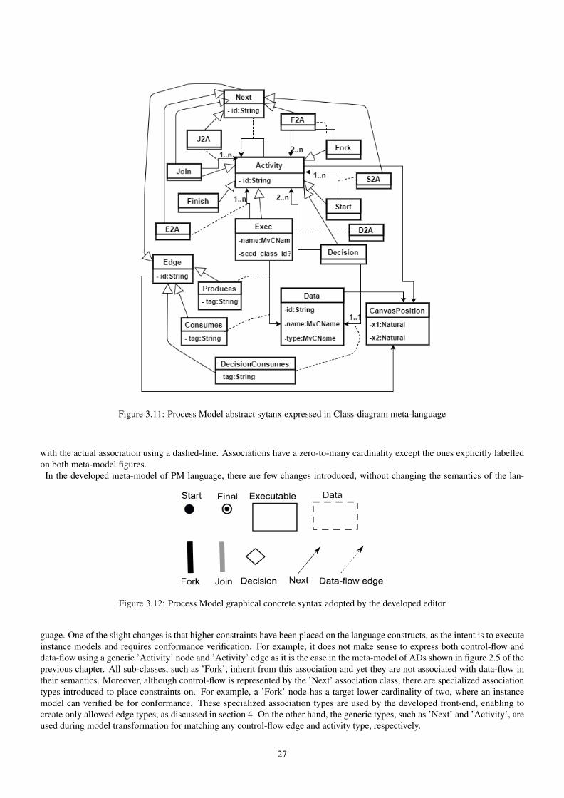
Figure 3.11: Process Model abstract sytanx expressed in Class-diagram meta-language

with the actual association using a dashed-line. Associations have a zero-to-many cardinality except the ones explicitly labelledon both meta-model figures.

In the developed meta-model of PM language, there are few changes introduced, without changing the semantics of the lan-

Figure 3.12: Process Model graphical concrete syntax adopted by the developed editor

guage. One of the slight changes is that higher constraints have been placed on the language constructs, as the intent is to executeinstance models and requires conformance verification. For example, it does not make sense to express both control-flow anddata-flow using a generic ’Activity’ node and ’Activity’ edge as it is the case in the meta-model of ADs shown in figure 2.5 of theprevious chapter. All sub-classes, such as ’Fork’, inherit from this association and yet they are not associated with data-flow intheir semantics. Moreover, although control-flow is represented by the ’Next’ association class, there are specialized associationtypes introduced to place constraints on. For example, a ’Fork’ node has a target lower cardinality of two, where an instancemodel can verified be for conformance. These specialized association types are used by the developed front-end, enabling tocreate only allowed edge types, as discussed in section 4. On the other hand, the generic types, such as ’Next’ and ’Activity’, areused during model transformation for matching any control-flow edge and activity type, respectively.

27

Figure 3.13: Statecharts abstract syntax expressed in Class-diagram meta-language.

Figure 3.14: SCCD graphical concrete syntax adopted by the developed editor

Some of the introduced changes are also used to adopt to the developed Graphical User Interface (GUI) editor, as it is alsothe case for SCCD meta-model. These updates include additional entities, such as ’CanvasPosition’, which saves the positionof element on the editor’s canvas and can be used for rendering models from the repository back to the editor. Note that theModelverse is also a model repository and uses the abstract syntax of a language as data structure to save models. The graphicalconcrete syntax of Statecharts in SCCD, as depicted on figure 3.14, looks a bit different than Harel’s first representation, shownin chapter 2. These changes took place as an alternative choice, and include highlighting of initial states in colour rather than

28

a small uni-directional edge targeting the state. In addition, hierarchical states are not rounded rectangles. A ’Parallel’ state isrepresented by a dashed-line rectangle, with ’Composite’ states as its orthogonal components. The developed concrete syntaxof the PM language also adopts to UML 2.0 ADs with a slight change that enables a clear distinction between ’Join’ and ’Fork’nodes as well as a different representation for data nodes, as shown in figure 3.12.

3.3.2 Model Transformation of PM to SCCD

The Modelverse enables the creation of model operations as models themselves, allowing several language instances to be exe-cuted. In this case, the model operation takes, as input, an instance of PM and SCCD, and produce one SCCD model instance thatincludes the Orchestrator SCCD. As discussed in the previous chapter, the Modelverse has support for both types of commonlyused model operation approaches, model transformations through RAMification and explicitly modelled action language. Whilemapping PM constructs onto SCCD with the chosen approach, there is a tedious task of identifying order, i.e. the precedingand/or successor element of PM activities and data nodes being mapped. This implementation, thereby, uses model transforma-tions through RAMification, as it can take advantage of the very intuitive (i.e. explicitly modelled) pattern searching method.In addition, note from the abstract syntax meta-model of the PM language in figure 3.11, an ’Activity’ is a generic entity as allnodes, expect ’Data’, inherit from it. Similarly, the association ’Next’ is a generic edge denoting control-flow edges of a PM.Hence, the implemented model transformation uses these generic types to search for pattern matches, which reduces the numberof rules required for mapping the constructs.The mapping of PM instance onto SCCD model consists of multiple transformation rules and enclosing of these rules in a chosenrule-block. The rule-blocks are then scheduled for execution, as depicted in the code fragment shown in figure 3.1. The rules andtheir scheduling are implemented using a textual concrete syntax, which the Modelverse only supports at this time. However,graphical illustrations of some of the rules discussed are provided here for readability. In addition, all executable code fragmentsare written in neutral action language code, which the Modelverse has an interpreter for.

Initial (schedule , create_orchestrator) {}

OnSuccess (create_orchestrator , create_association) {}OnSuccess (create_association , ModifyFork2Fork) {}OnSuccess (ModifyForkToFork , ModifyForkToFork) {}OnSuccess (RemoveForkToFork , RemoveJoinToJoin) {}OnSuccess (RemoveJoinToJoin , initialize) {}OnSuccess (initialize , data_produces) {}OnSuccess (map_exec , map_decision) {}OnSuccess (data_produces , data_consumes) {}OnSuccess (data_consumes , compile_init_script) {}OnSuccess (map_decision , map_fork) {}OnSuccess (map_fork , map_join) {}OnSuccess (map_join , map_finish) {}OnSuccess (map_finish , map_start) {}OnSuccess (map_start , success) {}

OnFailure (create_orchestrator , create_association) {}OnFailure (create_association , ModifyFork2Fork) {}OnFailure (ModifyForkToFork , RemoveForkToFork) {}OnFailure (RemoveForkToFork , RemoveJoinToJoin) {}OnFailure (RemoveJoinToJoin , initialize) {}OnFailure (initialize , data_produces) {}OnFailure (map_exec , map_decision) {}OnFailure (data_produces , data_consumes) {}OnFailure (data_consumes , compile_init_script) {}OnFailure (map_decision , map_fork) {}OnFailure (map_fork , map_join) {}OnFailure (map_join , map_finish) {}OnFailure (map_finish , map_start) {}OnFailure (map_start , success) {}

Listing 3.1: Schedule of model transformation rules used for mapping PM to SCCD

This schedule exposes a number of steps starting at the ’Initial’ step, where it has the first rule as a second parameter, i.e.’create orchestrator’. Each step is connected to two other steps with an ’OnSuccess’ or ’OnFailure’ function. Hence, each rulein this case is an entry as a parameter on both steps where execution can follow. For example, the first rule (’create orchestrator’)is a parameter on both functions such that if execution finds a match or not the next rule to execute is ’create association’.The first rule is used to create the Orchestrator SCCD, and is enclosed in an Atomic rule-block, and it is depicted on figure 3.15.This rule searches for the SCCD diagram entity in the LHS and adds a new SCCD (the Orchestrator) to the diagram on the

29

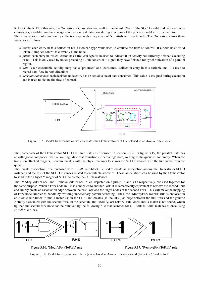
RHS. On the RHS of this rule, the Orchestrator Class also sets itself as the default Class of the SCCD model and declares, in itsconstructor, variables used to manage control-flow and data-flow during execution of the process model it is ’mapped’ to.These variables are of a dictionary collection type with a key entry of ’id’ attribute of each node. The Orchestrator uses thesevariables as follows:

• token: each entry in this collection has a Boolean type value used to emulate the flow of control. If a node has a validtoken, it implies control is currently at the node.• finish: each entry in this collection has a Boolean type value used to indicate if an activity has currently finished executing

or not. This is only used by nodes preceding a Join construct to signal they have finished for synchronization of a parallelregion.• data: each executable activity entry has a ’produces’ and ’consumes’ collection entry in this variable and it is used to

record data-flow in both directions.• decision consumes: each decision node entry has an actual value of data consumed. This value is assigned during execution

and is used to dictate the flow of control.

Figure 3.15: Model transformation which creates the Orchestrator SCCD enclosed in an Atomic rule-block

The Statecharts of the Orchestrator SCCD has three states as discussed in section 3.1.2. In figure 3.15, the parallel state hasan orthogonal component with a ’waiting’ state that transitions to ’creating’ state, so long as the queue is not empty. When thetransition attached triggers, it communicates with the object manager to spawn the SCCD instance with the first name from thequeue.The ’create association’ rule, enclosed with ForAll rule-block, is used to create an association among the Orchestrator SCCDinstance and the rest of the SCCD instances related to executable activities. These associations can be used by the Orchestratorto send to the Object Manager of SCCD to create the SCCD instances.The ’ModifyForkToFork’ and ’RemoveForkToFork’ rules, depicted on figure 3.16 and 3.17 respectively, are used together forthe same purpose. When a Fork node in PM is connected to another Fork, it is semantically equivalent to remove the second Forkand simply create an association edge between the first Fork and the target nodes of the second Fork. This will make the mappingof Fork node simpler to handle by avoiding unnecessary pattern searching. Thus, the ’ModifyForkToFork’ rule is enclosed inan Atomic rule-block to find a match (as in the LHS) and creates (in the RHS) an edge between the first fork and the genericActivity associated with the second fork. In the schedule, the ’ModifyForkToFork’ rule loops until a match is not found, whichby then the second fork node can be removed by the following rule that searches for all ’Fork-to-Fork’ matches at once usingForAll rule-block.

Figure 3.16: ’ModifyForkToFork’ rule Figure 3.17: ’RemoveForkToFork’ rule

Figure 3.18: Model transformation rule in (a) enclosed in Atomic rule-block and (b) in ForAll rule-block

30

Node Type Variable Initial ValueStart token[id] True

Decision token[id] Falsedecision consumes[id] None

Join finish[preceding node id] False

Exectoken[id] Falsedata[id][’consumes’] Empty Listdata[id][’produces’] Empty List

Fork/Finish token[id] False

Table 3.1: Initial configuration of variable instances of the Orchestrator SCCD

Similarly, the ’RemoveJoinToJoin’ rule searches for all matches where a Join node has a direct association with another Join, andthat the second one is connected to a generic Activity. Again, it is semantically equivalent to remove the second join node andcreate a new association between the first Join node and the generic Activity.

The ’initialize’ rule has, in the LHS, a basic state (i.e. the initial state of the Orchestrator SCCD) and a generic activity in PM.This rule is enclosed in a ForAll rule-block to find a match equivalent to the Cartesian product of the basic state and all nodesrepresented by the generic activity type. For every match found, based on its actual type, it initializes the variables of the Orches-trator in the RHS. The configuration of variables based on the activity type is shown in table 3.1. Note that node ’id’ attribute isused as a key entry, and if the generic activity is of type Join, all its preceding nodes will have an entry in the ’finish’ variable aswell.

The ’map exec’ rule, as shown in the LHS of figure 3.19, searches for all matches with a pattern having an executable type

Figure 3.19: Model transformation rule enclosed in a ForAll rule-block for mapping an Executable activity to an orthogonalcomponent in the Orchestrator SCCD parallel state.

connected to a generic activity node using a generic control-flow edge. The search also includes the parallel state in the Orches-trator SCCD. For each match found, it adds a new orthogonal component in the parallel state and configures the attributes ofstates and transition created. The transition’s ’guard’ attribute is set for a valid token and the ’script’ attribute is defined as thesuccessor activity (in the RHS) being assigned a valid token. The orthogonal component is mapped to the executable constructwith a traceability link. This link can be used by other successor rules in the schedule for searching new patterns created duringmodel transformations. In addition, they can be used in debugging operation by providing a trace to the mapping of constructsbelonging to different model instances. The orthogonal component has two states describing the behaviour of the SCCD instancean executable activity corresponds to, and it is discussed in section 3.1.2.The two rules related to data-flow, namely ’data produces’ and ’data consumes’, have a similar purpose. In the LHS, the rules

search for all matches satisfying the pattern where an executable activity connected to a data node is found. This edge is anoutgoing edge for ’data produces’ rule and an incoming edge for ’data consumes’. There is also a search for the initial state ofthe Orchestrator SCCD, as shown in the code snippet in figure 3.2. Note that the constraint on the LHS is used to identify theinitial basic state of the Orchestrator SCCD, as there can be multiple instances of basic states in the input model. For each matchfound, in the RHS, it uses the initial state of the Orchestrator to initialize, in its OnEntryScript attribute, the data variable instanceused to record meta-data of models in both directions.The ’map decision’ rule has in its LHS a pattern search for the parallel state of the Orchestrator SCCD and data node connectedto a decision using the ’DecisionConsumes’ association edge. This association has a constraint defined in the abstract syntax ofthe PM language, which makes it a binding requirement for a decision node to consume exactly one data. For each match found,in the RHS it adds a new orthogonal component with a child basic state inside the Orchestrator Parallel state, and configures the

31

Figure 3.20: Model transformation rule enclosed in ForAll rule-block used for mapping Fork to an orthogonal component in theOrchestrator SCCD parallel state

decision consumes variable instance. This variable is assigned a value based on the run-time result of data (model attribute) thedecision node consumes. The basic state in the orthogonal component has a transition targeting itself. This transition’s ’guard’attribute is set for a valid token and the ’script’ attribute is defined as the successor activity (in the RHS) being assigned a validtoken. The orthogonal component child state describes the behaviour of a decision node it is mapped to, as discussed in section3.1.2.

{Contains} ForAll data_produces {LHS {

Pre_PM/Exec pre_0 {label = "0"

}Pre_PM/Data pre_1 {

label = "1"}Pre_PM/Produces pre_2 (pre_0 , pre_1) {

label = "2"}Pre_SCCD/BasicState pre_3 {

label = "3"}constraint = $

Boolean function constraint (model : Element , mapping : Element):Element childrenString parentElement class_behString classchildren = allIncomingAssociationInstances(model , mapping["3"], "SCCD/

composite_children")if list_len(children) >0:

parent = readAssociationSource(model , set_pop(children))class_beh = allIncomingAssociationInstances(model , parent , "SCCD/behaviour")if list_len(class_beh) >0:

class = readAssociationSource(model , set_pop(class_beh))if (value_eq(read_attribute(model , class , "name"), "Orchestrator")):

return True!else:

return False!else:

return False!else:

return False!$

}RHS {

Post_PM/Exec post_0 {label = "0"

}Post_PM/Data post_1 {

label = "1"}Post_PM/Produces post_2 (post_0 , post_1) {

label = "2"

32

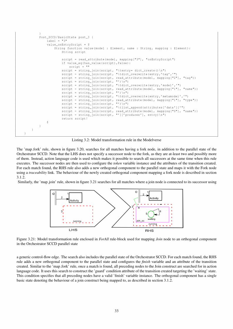
}Post_SCCD/BasicState post_3 {

label = "3"value_onEntryScript = $

String function value(model : Element , name : String , mapping : Element):String script

script = read_attribute(model , mapping["3"], "onEntryScript")if value_eq(has_value(script),False):

script = ""script = string_join(script , "\tentry= dict_create()\n")script = string_join(script , "\tdict_overwrite(entry ,’tag ’,’")script = string_join(script , read_attribute(model , mapping["2"], "tag"))script = string_join(script , "’)\n")script = string_join(script , "\tdict_overwrite(entry ,’model ’,’")script = string_join(script , read_attribute(model , mapping["1"], "name"))script = string_join(script , "’)\n")script = string_join(script , "\tdict_overwrite(entry ,’metamodel ’,’")script = string_join(script , read_attribute(model , mapping["1"], "type"))script = string_join(script , "’)\n")script = string_join(script , "\tlist_append(attributes[’data ’][’")script = string_join(script , read_attribute(model , mapping["0"], "name"))script = string_join(script , "’][’produces ’], entry)\n")return script!

$}

}}

Listing 3.2: Model transformation rule in the Modelverse

The ’map fork’ rule, shown in figure 3.20, searches for all matches having a fork node, in addition to the parallel state of theOrchestrator SCCD. Note that the LHS does not specify a successor node to the fork, as they are at-least two and possibly moreof them. Instead, action language code is used which makes it possible to search all successors at the same time when this ruleexecutes. The successor nodes are then used to configure the token variable instance and the attributes of the transition created.For each match found, the RHS rule also adds a new orthogonal component to the parallel state and maps it with the Fork nodeusing a traceability link. The behaviour of the newly created orthogonal component mapping a fork node is described in section3.1.2.Similarly, the ’map join’ rule, shown in figure 3.21 searches for all matches where a join node is connected to its successor using

Figure 3.21: Model transformation rule enclosed in ForAll rule-block used for mapping Join node to an orthogonal componentin the Orchestrator SCCD parallel state

a generic control-flow edge. The search also includes the parallel state of the Orchestrator SCCD. For each match found, the RHSrule adds a new orthogonal component to the parallel state and configures the finish variable and an attribute of the transitioncreated. Similar to the ’map fork’ rule, once a match is found, all preceding nodes to the Join construct are searched for in actionlanguage code. It uses this search to construct the ’guard’ condition attribute of the transition created targeting the ’waiting’ state.This condition specifies that all preceding nodes have a valid ’finish’ variable instance. The orthogonal component has a singlebasic state denoting the behaviour of a join construct being mapped to, as described in section 3.1.2.

33

4Visual Editor

An application front-end is developed for both languages (PM and SCCD) which uses their graphical concrete syntax and es-sentially enables for visually modelling workflows at different levels of abstraction. This GUI editor consists of mainly twoparts, one that make up for a PM editor and the other for SCCD. Hence, the overall goal was to obtain a user-friendly modellingenvironment which integrates the two languages and interacts with the Modelverse. The Modelverse [22], serves as a modelrepository in addition to being a multi-paradigm modelling and simulation back-end. This section discusses the design choicesmade during development, followed by highlighting essential functional requirements incorporated in both parts of the editor.

4.1 Design Choices and Application Architecture

The developed front-end application has high interactive features with complex user interface (UI) requirements, such as multipleinstantiation of an element on canvas, hierarchical layering of constructs and drag and drop of such constructs. This and manymore complex features of the editing environment requires to explicitly model its behaviour. Thus, SCCD is chosen as an appro-priate formalism given the UI can be characterized with a behaviour that is reactive, timed, autonomous and dynamic- structure.In the implementation, SCCDXML [19], which is a textual concrete syntax of SCCD, is used. In addition, the application front-end utilizes external libraries to implement non functional requirements. These libraries include mainly widgets from Python’sTkinter [4] package, i.e. a GUI programming toolkit.

Figure 4.1: An overview of the implemented application architecture.

34

The application architecture can be summarized in figure 4.1. The Application front-end Module consists of SCCD classes andtheir Statecharts for modelling the behaviour of the UI. For example, figure 4.1 depicts a code fragment of the SCCDXML used toexplicitly model all instances of a ’Button’ entity. This SCCD class inherits from Tkinter’s Button widget and, in its constructor,instantiates it to create a button for the associated ”Toolbar” SCCD.

1 <c l a s s name=” B u t t on ”>2 < r e l a t i o n s h i p s>3 <a s s o c i a t i o n name=” p a r e n t ” c l a s s =” T o o l b a r ” />4 < i n h e r i t a n c e c l a s s =” wi dg e t ” p r i o r i t y = ’ 0 ’ />5 < i n h e r i t a n c e c l a s s =” t k . Bu t ton ” p r i o r i t y = ’ 1 ’ />6 < / r e l a t i o n s h i p s>7 <c o n s t r u c t o r>8 <p a r a m e t e r name=” c o n s t r u c t o r p a r a m e t e r s ” t y p e = ’ d i c t ’ d e f a u l t = ’ {} ’ />9 <s u p e r c l a s s =” t k . B u t t on ”>

10 <p a r a m e t e r exp r =” c o n s t r u c t o r p a r a m e t e r s [ ’ p a r e n t ’ ] ” />11 <p a r a m e t e r exp r =” ∗∗ ( c o n s t r u c t o r p a r a m e t e r s [ ’ v i s u a l ’ ] . g e t p a r a m s ( ) ) ” />12 < / s u p e r>13 <s u p e r c l a s s =” w id ge t ” />14 <body>15 s e l f . l a b e l = c o n s t r u c t o r p a r a m e t e r s [ ” e v e n t p a r a m e t e r s ” ]16 < / body>17 < / c o n s t r u c t o r>18 <d e s t r u c t o r>19 <body>s e l f . d e s t r o y ( )< / body>20 < / d e s t r u c t o r>21 <scxml i n i t i a l =” main ”>22 < s t a t e i d =” main ” i n i t i a l = ’ i n i t i a l i z i n g ’>23 < s t a t e i d =” i n i t i a l i z i n g ”>24 < t r a n s i t i o n e v e n t = ’ s e t a s s o c i a t i o n n a m e ’ t a r g e t =” . . / r u n n i n g ”>25 <p a r a m e t e r name= ’ a s s o c i a t i o n n a m e ’ t y p e = ’ s t r ’ />26 < s c r i p t>s e l f . a s s o c i a t i o n n a m e = a s s o c i a t i o n n a m e< / s c r i p t>27 < / t r a n s i t i o n>28 < / s t a t e>29 < s t a t e i d =” r u n n i n g ”>30 < t r a n s i t i o n p o r t = ’ i n p u t ’ e v e n t =” l e f t −c l i c k ” t a r g e t = ’ . ’ cond= ’ t a g o r i d == i d ( s e l f ) ’>31 <p a r a m e t e r name= ’ t a g o r i d ’ t y p e = ’ i n t ’ d e f a u l t = ’ None ’ />32 < r a i s e e v e n t =” b u t t o n p r e s s e d ” scope =” nar row ” t a r g e t =” ’ p a r e n t ’ ”>33 <p a r a m e t e r exp r =” s e l f . l a b e l ” />34 < / r a i s e>35 < / t r a n s i t i o n>36 < t r a n s i t i o n p o r t = ’ i n p u t ’ e v e n t =” e n t e r ” t a r g e t = ’ . ’ cond= ’ t a g o r i d == i d ( s e l f ) ’>37 <p a r a m e t e r name= ’ t a g o r i d ’ t y p e = ’ i n t ’ d e f a u l t = ’ None ’ />38 < s c r i p t>39 s e l f . t o o l t i p . s h o w t i p ( )40 < / s c r i p t>41 < / t r a n s i t i o n>42 < t r a n s i t i o n p o r t = ’ i n p u t ’ e v e n t =” l e a v e ” t a r g e t = ’ . ’ cond= ’ t a g o r i d == i d ( s e l f ) ’>43 <p a r a m e t e r name= ’ t a g o r i d ’ t y p e = ’ i n t ’ d e f a u l t = ’ None ’ />44 < s c r i p t>45 s e l f . t o o l t i p . h i d e t i p ( )46 < / s c r i p t>47 < / t r a n s i t i o n>48 < / s t a t e>49 < / s t a t e>50 < / scxml>51 < / c l a s s>

Listing 4.1: SCCD instance of a Button type used for developing the visual editor expressed in SCCDXML notation

The Statecharts of this SCCD model is enclosed with <scxml> tag, and in there, we can see that the state with id ’running’ hasa transition with an event ’left-click’. When this transition triggers, it will raise an event with a narrow scope to the associatedToolbar SCCD and sends as a parameter a unique identifier (name) of the Button instance. The transition also listens to an ’enter’and/or ’exit’ events where upon triggering calls a method of the inherited ’Widget’ external class which visually shows a tooltipfor the button instance. The associated Toolbar SCCD, with an association name ’parent’, is the one responsible for the creationand deletion of a Button SCCD instance.The application front-end essentially interacts with a wrapper to the Modelverse, i.e. the Repository Application ProgrammingInterface (API). This wrapper initially connects to the Modelverse (via HTTP) and provides a high-level interface which initiatescalls to the Modelverse that perform operations on models found in the repository. These operations mainly include creating,fetching, updating and deleting of relevant data pertaining to both model types (PM and SCCD). The Application front-end

35

module includes SCCDs which relate to the simulation interface developed. Thus, these classes serve as an interface to interactwith the SCCD Simulation Engine to visually characterize the run-time behaviour of the application. Note that the SCCDsimulator is in the Modelverse and has access to SCCD models. The Serializer API can optionally be used to generate SCCDXMLfrom SCCD models in the Modelverse. A compiler already exists for SCCDXML and can be used to generate executable codefor multiple platforms, such as Python, javaScript, and CSharp.

4.2 Process Model Editor

When the application launches, the PM editor part of the application front-end is presented to the user. As depicted on figure4.2, the editor window consists of a toolbar and a canvas. The labels on the toolbar include PM modelling constructs. When thetoolbar loads these constructs, it requests for all types defined in the abstract syntax meta-model, via the Modelverse wrapper(Repository API). The abstract syntax is depicted in figure 3.11 of the previous chapter. Thus, a label in the toolbar is createdif its type exists in the meta-model. In this manner the application front-end easily adopts to changes in the definition of themeta-model and enables to preserve consistency between the concrete syntax and abstract syntax of the modelling language.

Figure 4.2: The developed visual editor for PM.

The concrete syntax of the PM language includes nodes, i.e. activities (of six types) and data, and edges associating these nodes.When edges are created, the canvas requests for allowed connection types based on the definition of the abstract syntax meta-model. This procedure involves requesting the Modelverse, via the repository API, for all association types between source andtarget constructs selected while creating an edge. If the result returned is empty, the user is prompted with an error messageindicating no association exists for the selected source and target types. Similarly, if the result is a list of associations of sizegreater than one (such as the case for an executable activity and data), the user is prompted to select which association tocreate, as in figure 4.3. Otherwise, the association is automatically created given the result is only one. The abstract syntax hasspecialized associations that inherit from the generic ’Next’ association which represents control-flow. These associations areused to constrain the user to create allowed connection types in the front-end, as discussed above. Moreover, this way of creatingan association implies that the application front-end automatically adopts to modifications in the definition of the modelling

36

language abstract syntax, such as creating a new association type or deleting an existing one.The graphical concrete syntax of the PM developed in this editor essentially provides a clear distinction among these variousconstructs. Data nodes and edges representing data-flow are created using dotted-lines. Similarly, a Join node and a Fork nodehave different visual representation, as opposed to the UML 2.0 AD’s concrete syntax which makes no distinction between thesetwo types.Nodes can be created on canvas and positioned as desired. While positioning, using a drag-and-drop behaviour, an associated

Figure 4.3: Prompting user for selecting association types defined in the abstract syntax of PM

edge (if any) is also automatically animated following the position of a node. When creating an edge, the user can be able tooptionally add multiple in between angle points (control points) used to edit the position of the edge. The developed GUI providesseparate windows for editing the attributes of a given construct. After editing an edge attributes, their values are displayed aslabels on the edges, such as the one for data-flow edges or outgoing edges of a Decision node.The application front-end also enables for rendering models on canvas from the repository. While loading a selected modelinstance, the constructs are placed on canvas preserving their last position saved.

4.3 SCCD Editor

As discussed in the previous chapters, SCCD models are encapsulated in PM executable activities. Hence, an instance of theSCCD editor is launched when an executable activity is selected with a double-click event. At this time, the application front-enduses the repository API to inquire which SCCD class is mapped to the activity and ultimately presents it on the editor, as shownin figure 4.4. The SCCD class can be positioned on canvas as desired and also has a separate window with input fields to updateits attributes. These attributes are optional and include attributes, methods, constructor, and a destructor. The name propertywhich is disabled, is by default set to the name of the executable activity the SCCD relates to. Class methods can be created in aseparate window and has input fields for the name, parameters, body and return type attributes of a method. The behaviour edge,with a dotted-line, is used to associate the Class with its Statecharts.

37

Figure 4.4: SCCD visual editor for Activity A in figure 4.2

The SCCD editor also enables to create modelling constructs on canvas and position them as desired. Positioning of constructsalso involves automatic positioning of associated edges and hierarchical children, if any. States can be connected via an edge,namely a Transition edge. Since Statecharts have four modelling constructs, the concrete syntax developed for this editor essen-tially provides clear distinction among them. In addition, Statecharts also adds a notion of hierarchy and this is represented in theeditor with the most user intuitive manner. A state can be dragged into another state supporting hierarchy and be dropped. At thistime, the parent state automatically adjusts its size to accommodate the new child, and creates a semi-transparent line (shown inyellow dotted-line on figure 4.4) to emphasize the child-parent relationship.The SCCD editor enables to update settable properties of a state that includes its name and whether or not it is a default state.The latter is only available if the parent is not a Parallel state. If the state is a default one, the editor changes its appearance bypainting its edge with a green colour, as shown in figure 4.4. The state attributes editor window, shown in figure 4.5, has inputfields to define entry and exit actions for a state. As a state can have an unlimited number of raise events, it can be added byclicking the Add button. A separate pop-up window then appears with input fields for an event, scope and target attributes aswell as the option to add parameters. For a History state, there is a radio-button to select its type between shallow and deep.

38

Figure 4.5: State attributes editor in SCCD

Similarly, a transition editor window has input fields to set a its attributes including an event, guard, and after. Furthermore,there is an option to add formal event parameters and a raise entry associated to a transition. A transition has a label displayinga limited number of characters of its properties in the format T[C] / R[A], where T is the trigger, C a condition, R raised events,and A the action. When creating a transition, the user can be able to optionally add multiple in between angle points (controlpoints) used to edit the position of the edge, as depicted on figure 4.6.

Figure 4.6: Multiple angle points of an edge used for editing its position

Finally, the editor canvas has zooming capabilities to optimally utilize the diagram layout and make the editor scalable for largemodels. Similar to the PM editor, SCCD models can also be rendered on canvas from the repository. While loading, the instancemodel constructs are placed in their last position saved.

39

5Example

In this chapter, we will demonstrate the semantics of PM given in SCCD, by applying the power window case study discussedin chapter 2. In addition, unlike the process model previously discussed for the power window case, this instance of PM hasan activity responsible for obtaining an external service. Thus, we will also discuss this activity’s behaviour encapsulated in anexplicitly modelled SCCD.

Figure 5.1: A process model developed in the visual editor for the power window case study.

40

5.1 Case Study

The example we use is the power window case study discussed in chapter 2, however with slight changes. Figure 5.1 depicts thePM of this example using the developed visual editor and includes automatic operations and the models used by these operations.Note that manual operations are not included, as the process is only used for demonstrating the semantics of PM given in SCCD.All DSMLs and model instances in the FTG are pre-loaded to the Modelverse during environment setup.

As discussed in chapter 2, the intention of the PM in 5.1 is on the verification aspect of the power window, i.e. the window shouldnever go up when an object is inserted through. In that regard, the PM control-flow originates with a concurrent behaviour wheremodel transformations of instance models, such as Plant, are mapped to Encapsulated Petri-nets (EPNs). These operations aresynchronized by the Combine operation which consumes the EPNs and the Architecture model to produce a combined markedPetri-net model. This model in combination with a safety query model is subsequently used by the ’Analyse’ activity, which rep-resents an external service. The external service is not declared in the FTG, and the service obtained is an optimized reachabilityanalysis of the combined Petri-net model on a state predicate specified by the safety query model, as shown in figure 5.1. If thequery is found, the user is presented with a path from the Petri-net model that demonstrates why an unsafe situation is reached.Otherwise, the system is deemed safe, and the process terminates.

The behaviour of all executable activities in the PM is explicitly modelled in SCCD. In addition, the PM itself is mapped toSCCD, as discussed in chapter 3. The model operation, responsible for this mapping, takes as input the PM and the SCCD modelwhich expresses the behaviour of each executable activity in the PM. Following its execution, the model operation yields a singleSCCD model that includes the Orchestrator SCCD instance where the PM is mapped to. This output SCCD model, depicted onfigure 5.2, is then simulated. Since the output model is a result of automatic model operation, it does not have data about canvasposition of constructs to render on the developed visual editor.

41

Figure 5.2: The executable SCCD model generated after mapping PM to the Orchestrator SCCD

42

We can see that the Statecharts of the Orchestrator Class has, in its parallel state, orthogonal components which are mapped toall activity types in the PM and uses them to manage control-flow and data-flow. As discussed in chapter 3, note the conditionfor a valid ’token’ set upon the transitions attached to the initial state of these orthogonal components. When triggered, if theorthogonal component is a mapping for an executable activity, such as plant to EPN, it places its name in a ’queue’ to be created.The ’CreateSCCD’ orthogonal component has a transition attached to its initial state which gets triggered so long as the queueis not empty. At this time, it gets the name of the executable activity from the ’queue’ and raises an event to the object managerfor creating the SCCD instance corresponding to the activity with an identical name. The SCCD instance, by default, gets thename of the executable activity at design time in the visual editor. The ’running’ state is then entered and waits until the SCCDinstance informs of its termination by listening to an event on the attached transition, i.e. ’terminated’ event. Upon triggering,this transition takes an action which then passes the ’token’ to the successor node.In addition, when orthogonal components mapped to an executable type enter the ’running’ state, the transition targeting itselfhas an event ’load data’ that it listens to, which is a data request from the running SCCD instance. When triggered, the transitionraises an event to send the appropriate data related to the executable activity. The data management, as discussed in chapter3, takes place while mapping the PM to SCCD in the model transformation. In that regard, when the Orchestrator Statecharsenters the parallel state, where it manages the process flow, it remains well informed of which data is to be consumed and/orproduced by which executable activity. Hence, transitions in orthogonal components make use of the data variable instance ofthe Orchestrator Class to extract the appropriate data related to the executable in which the orthogonal component is mapped to.

Figure 5.3 depicts a run-time behaviour of the Combine executable activity, modelled in SCCD. In the Statecharts, there are

Figure 5.3: The behaviour of Combine activity in figure 5.1 modelled in SCCD

two types of model operations. The first one is for general model management purpose, represented by the basic states ’merge’and ’split’, for model merging or splitting respectively. While the other is responsible for model operations which depend on thesemantics of the languages of models consumed and produced by the operations. These operations in figure 5.3 are representedby the basic states ’merge to EPN’ and EPN to PN. Upon initialization of the Statecharts, the initial state requests for data tobe used by the operations. The transition attached to the initial state listens to receive data from the Orchestrator SCCD. Whentriggered, the transition takes an action to get the actual models based on the data received, and merges them before the modeloperation in invoked in the ’merge to EPN’ or EPN to PN states. After entering these states a model transformation gets exe-cuted after RAMification of the meta-models, as discussed in chapter 2. The transformation expects as a result a Boolean value.If the result is False, the state transitions to a ’failure’ state where it prompts the user with an error message. Otherwise, aftersplitting and saving the output models, the state transitions to the ’terminating’ state, where it raises an event to notify the mappedorthogonal component in the parallel state of the Orchestrator SCCD instance. The behaviour of model operations declared inthe FTG is almost similar to the one discussed now. In the PM, ’merge to EPN’ and ’print path’ operations are defined in neutralaction language code, while the others use model transformation through RAMification. In the following section, we will discussthe behaviour of the PM activity Analyse, which is explicitly modelled in SCCD and is responsible for external service interaction.

5.2 External Service Interaction

The Modelverse has a complete support of the FTG+PM framework as illustrated in the power window case study in chapter2. In the FTG, there are various model operations defined there in, such as the one for conducting reachability analysis of a

43

Petri-net model. The reachability graph, from a marked Petri-net model, is developed first by using action language. This graph,coupled with a query model specifying the state predicates, are used as input models to a model operation which performs thereachability analysis. Although this method is feasible and already enacted, performance issues can still be at stake and obtainingan optimized reachability analysis is desirable.Thus, we used the service of LoLA, which is a Petri net model analyzer tool available external to the Modelverse environment.LoLA [13] (a Low Level Petri Net Analyzer) has been implemented for the validation of reduction techniques for Petri-netreachability graphs. Most properties supported by LoLA can be specified in temporal logic, either using branching time logicCTL or the linear time logic LTL. Instead of running a general LTL or CTL model checking algorithm, LoLA first checks whetherthe property can be reduced to a search for the desired property, i.e. in this case a simple reachability query. If so, it runs anoptimized state space exploration technique, such as partial order reduction (the stubborn set method), to that particular property.Stubborn set computation abides to rules ensuring the desired properties are preserved in the reduced state space.

5.2.1 Implementation

The Modelverse itself runs as a service, and enables for other (external) services to connect and to communicate data. An externalservice is required to connect (via HTTP) and register first before exchanging data with a client of the Modelverse. Once regis-tered, the client can connect to the registered service which allows for synchronous data transfer protocol. LoLA does not requireany user interaction (except for aborting execution) and purely works in batch mode. Its input and output can be organized bygenerating files, or it allows to read from standard input and write to standard output.

LoLA expects, as its input, a Petri-net model in a clearly arranged ASCII based language. It uses proprietary file formats whichis simple to generate and easy to parse. LoLAs Petri-net file formats contains of three main parts as follows [13]:

• Places are defined as a comma-separated list of place names, beginning with keyword PLACE. Optionally, for a list (sub-list) of places, a token bound (capacity) can be defined using keyword SAFE followed by a number, 1 being the default. Ifa place is listed several times, the respective arc weights are added.• An initial marking begins with keyword MARKING followed by a list of comma-separated assignments of token numbers

to place names. An initial marking of one is assumed if only a place name is listed.• A transition list begins with keyword TRANSITION, followed by a name and an optional fairness assumption (STRONG

FAIR or WEAK FAIR). Then, the transitions preset (CONSUME) and postset (PRODUCE) is given similar to a marking.An arc weight of 1 is assumed if not given explicitly.

The extended BackusNaur form (EBNF) grammars of this file format is provided in figure 5.4.A serializer is implemented (in action language) which translates a Petri-net model, in the Modelverse, to a format which uses the

Figure 5.4: EBNF grammars of LoLA’s file format.

EBNF grammars of LoLA. In addition, the serializer also translates the Query model specifying the state predicate to a temporallogic formula to be used by LoLA. The output of this serialization is again encoded in a JSON format which can be transferredover a network. A wrapper for LoLA is also implemented which decodes the JSON input and invokes LoLA by providing itsparameters, i.e. the input Petri-net model and state predicate.After analysis is made, LoLA supports its results by providing a path from the initial marking to a marking that demonstrateswhy the property is (not) satisfied. This and other relevant data, such as reports in run time and size of the explored part of thestate space, is provided as an output. The implemented wrapper uses this generated output to extract and send relevant data to

44

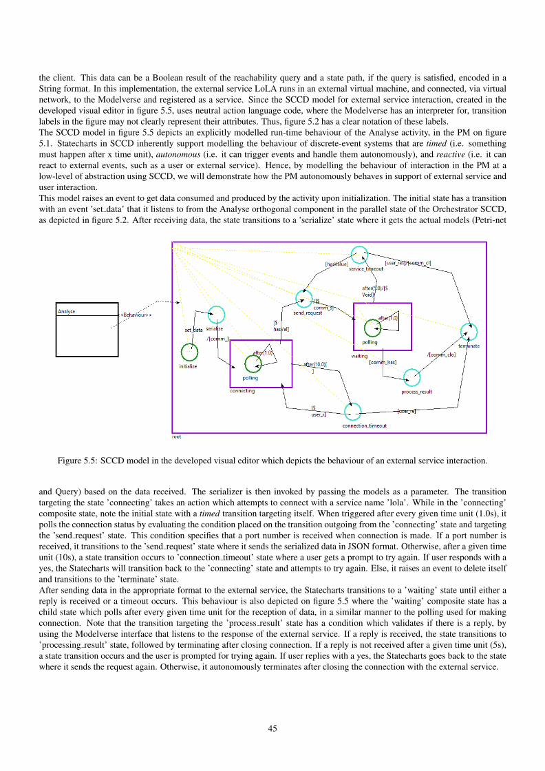
the client. This data can be a Boolean result of the reachability query and a state path, if the query is satisfied, encoded in aString format. In this implementation, the external service LoLA runs in an external virtual machine, and connected, via virtualnetwork, to the Modelverse and registered as a service. Since the SCCD model for external service interaction, created in thedeveloped visual editor in figure 5.5, uses neutral action language code, where the Modelverse has an interpreter for, transitionlabels in the figure may not clearly represent their attributes. Thus, figure 5.2 has a clear notation of these labels.The SCCD model in figure 5.5 depicts an explicitly modelled run-time behaviour of the Analyse activity, in the PM on figure5.1. Statecharts in SCCD inherently support modelling the behaviour of discrete-event systems that are timed (i.e. somethingmust happen after x time unit), autonomous (i.e. it can trigger events and handle them autonomously), and reactive (i.e. it canreact to external events, such as a user or external service). Hence, by modelling the behaviour of interaction in the PM at alow-level of abstraction using SCCD, we will demonstrate how the PM autonomously behaves in support of external service anduser interaction.This model raises an event to get data consumed and produced by the activity upon initialization. The initial state has a transitionwith an event ’set data’ that it listens to from the Analyse orthogonal component in the parallel state of the Orchestrator SCCD,as depicted in figure 5.2. After receiving data, the state transitions to a ’serialize’ state where it gets the actual models (Petri-net

Figure 5.5: SCCD model in the developed visual editor which depicts the behaviour of an external service interaction.

and Query) based on the data received. The serializer is then invoked by passing the models as a parameter. The transitiontargeting the state ’connecting’ takes an action which attempts to connect with a service name ’lola’. While in the ’connecting’composite state, note the initial state with a timed transition targeting itself. When triggered after every given time unit (1.0s), itpolls the connection status by evaluating the condition placed on the transition outgoing from the ’connecting’ state and targetingthe ’send request’ state. This condition specifies that a port number is received when connection is made. If a port number isreceived, it transitions to the ’send request’ state where it sends the serialized data in JSON format. Otherwise, after a given timeunit (10s), a state transition occurs to ’connection timeout’ state where a user gets a prompt to try again. If user responds with ayes, the Statecharts will transition back to the ’connecting’ state and attempts to try again. Else, it raises an event to delete itselfand transitions to the ’terminate’ state.After sending data in the appropriate format to the external service, the Statecharts transitions to a ’waiting’ state until either areply is received or a timeout occurs. This behaviour is also depicted on figure 5.5 where the ’waiting’ composite state has achild state which polls after every given time unit for the reception of data, in a similar manner to the polling used for makingconnection. Note that the transition targeting the ’process result’ state has a condition which validates if there is a reply, byusing the Modelverse interface that listens to the response of the external service. If a reply is received, the state transitions to’processing result’ state, followed by terminating after closing connection. If a reply is not received after a given time unit (5s),a state transition occurs and the user is prompted for trying again. If user replies with a yes, the Statecharts goes back to the statewhere it sends the request again. Otherwise, it autonomously terminates after closing the connection with the external service.

45

6Conclusion

In this thesis we assessed and demonstrated how it can be possible to model at multiple levels of abstractions to explicitly modelworkflow (process) behaviour such as concurrency, and essentially enact the Process Model (PM) itself. The semantics of a PMwas given in a low-level language, i.e. Statecharts Class-diagram (SCCD), where its semantic domain is already defined andsimulated. The PM used is a subset of the UML 2.0 Activity Diagrams, and in the context of Multi-paradigm Modelling (MPM),it is tightly coupled with the Formalism Transformation Graph, in the FTG+PM framework [9]. The PM describes, at a high-levelof abstraction, the flow of execution of model operations (as activities) applied on a set of formalisms (as data) declared in theFTG. PM activities can also coordinate with external services and/or users. Hence, activities in PM are enacted either throughtheir low level SCCD specification, or by calling upon external services. SCCD facilitates the specification of dynamic-structuresystems that are timed, autonomous and reactive. This enabled the orchestration of PM activities with an external service and/ora user, by explicitly modelling its behaviour in Statecharts.

In order to denotationally map PM onto SCCD, we explored two approaches and showed their benefits and setbacks. Althoughsequential mapping approach is relatively intuitive and easy to debug, as it leverages common design patterns in both languages,it fails to easily map process models with complex behaviour, such as the interleaving of branches in parallel regions. Hence, amore generic (complete) approach was used which makes it possible to map any PM instance that conforms to its meta-model.This generic approach fully utilizes concurrency in SCCD, and maps each PM activity type to an orthogonal component inside aparallel state. Control-flow of the process is then managed using the routing of a shared ”token”.Moreover, we applied the concept of soundness of workflow-nets [17] to identify undesired behaviour of PM, i.e. a control-flowwith a Fork branch exiting a parallel region before synchronizing. Although such PM conforms to the meta-model of UML2.0 Activity Diagrams, it can lead to process execution anomalies such as improper termination, where simultaneous multipleinstantiation of activities occur. Thus, a thorough verification of PM instances based on the soundness property of workflow-netsis proposed.

An integrated visual modelling environment was developed in Tkinter on top of the Modelverse [23]. This visual editor combinesthe graphical concrete syntax of both (PM and SCCD) languages and enables for modelling at multiple levels of abstractions.SCCD was also used to explicitly model the user interface behaviour of the developed editor. We have used the power windowcase study in [3][9], as an example to demonstrate the semantics of PM given in SCCD. In the case study, we also included anactivity in the PM which is responsible for interacting with an external service. This service is an optimal reachability analysisof a Petri-net model not available in the FTG. In addition, the external service tool, i.e. LoLA [13], is hosted in a differentenvironment than the Modelverse, and a virtual network was used for connection and data exchange. While interacting, the PMactivity, which is expressed in an explicitly modelled SCCD, autonomously handles its interactive behaviour, including lack ofservice response and/or connection timeouts.

6.1 Future Works

This thesis research can further be extended in the following manner:

46

• One of the common design patterns in both languages is hierarchical composition, which was not covered in the currentresearch. The composition of hierarchy in PM enables for a given independent process to be encapsulated in another pro-cess. This can be used to modularize multiple process models and have them composed together for a common particularmotive.• Expressing the semantics of PM using SCCD in the current research provided an actual concurrent simulation of activities

in a parallel region of PM. This means that SCCD instances, used to express activities in a parallel region of the correspond-ing PM, are created and executed concurrently. However, the Modelverse does not parallelize multiple model operationsin which the activities represent. Parallelizing model operations can allow for fully collaborative usage of the Modelverse.• In this research, PM instance can be verified for their conformance to the meta-model. However, process models which do

not conform to the soundness property of workflow-nets discussed in chapter 3, can result in anomalies during execution,such as improper termination. A through verification of process models using the soundness property of workflow-nets canessentially prevent undesired behaviour of PM during simulation.

47

Bibliography

[1] Behzad Bordbar, Luisa Giacomini, and D Holding. Uml and petri nets for design and analysis of distributed systems. InIEEE Conference on Control Applications, pages 610–615, 2000.

[2] Juan De Lara and Esther Guerra. Deep meta-modelling with metadepth. In In International Conference on ModellingTechniques and Tools for Computer Performance Evaluation, pages 1–20, 2010.

[3] Joachim Denil. Design, Verification and Deployment of Software Intensive Systems. Universiteit Antwerpen, FaculteitWetenschappen, Departement Wiskunde-Informatica, 2013.

[4] Python Software Foundation. Graphical user interfaces with Tk - documentation. https://docs.python.org/2/library/tk.html. Accessed: 2017-03-8.

[5] Vangheluwe Hans, Juan de Lara, and Pieter J. Mosterman. An introduction to multi-paradigm modelling and simulation.pages 9–20.

[6] David Harel. Statecharts : a visual formalism for complex systems. Science of Computer Programming, 8(3):231–274,1987.

[7] John Hopcroft and Jeffrey Ullman. Introduction to Automata Theory, Languages, and Computation. Addison-Wesley, 1979.

[8] Anneke Kleppe. The field of software language engineering. Software Language Engineering Lecture Notes in ComputerScience, pages 1–7, 2009.

[9] Levi Lucio, Sadaf Mustafiz, Joachim Denil, Hans Vangheluwe, and Maris Jukss. Ftg+pm: An integrated framework forinvestigating model transformation chains. Lecture Notes in Computer Science SDL 2013: Model-Driven DependabilityEngineering, pages 182–202, 2013.

[10] Tadao Murata. Petri nets: Properties, analysis and applications. Proceedings of the IEEE, 77(4):541–580, 1989.

[11] OMG. UML 2.0 superstructure specification. Technical report, Object Management Group, 2005.

[12] Grzegorz Rozenberg. Handbook of graph grammars and computing by graph transformation, volume 1. World ScientificPublishing Co., Inc, 1997.

[13] Karsten Schmidt. Lola a low level analyser. In IEEE Conference on Control Applications, pages 465–474, 2000.

[14] Harald Strrle, Jan Hendrik Hausmann, and Universitt Paderborn. Towards a formal semantics of uml 2.0 activities. InProceedings German Software Engineering Conference, volume P-64 of LNI, pages 117–128, 2005.

[15] Eugene Syriani, Jeff Gray, and Hans Vangheluwe. Modeling a model transformation language. In Domain Engineering,pages 211–237, 2013.

[16] Eugene Syriani, Hans Vangheluwe, Raphael Mannadiar, Conner Hansen, Van Mierlo, and Huseyin Ergin. Atompm: Aweb-based modeling environment, 2013.

[17] W. M. P. van der Aalst, K. M. Van Hee, A. H. M. Ter Hofstede, N. Sidorova, H. M. W. Verbeek, M. Voorhoeve, and M. T.Wynn. Soundness of workflow nets: Classification, decidability, and analysis. Formal Aspects of Computing, 23(3):333–363, 2011.

[18] Simon Van Mierlo. SCCD documentation. https://msdl.uantwerpen.be/documentation/SCCD/. Accessed: 2017-02-16.

[19] Simon Van Mierlo, Yentl Van Tendeloo, Bart Meyers, Joeri Exelmans, and Hans Vangheluwe. SCCD: SCXML extendedwith class diagrams. In 3rd Workshop on Engineering Interactive Systems with SCXML, part of EICS 2016, 2016.

48

[20] Simon Van Mierlo, Yentl Van Tendeloo, Bart Meyers, and Hans Vangheluwe. Domain-specific modelling for humancom-puter interaction. HumanComputer Interaction Series The Handbook of Formal Methods in Human-Computer Interaction,pages 435–463, 2017.

[21] Yentl Van Tendeloo. Modelverse’s documentation. https://msdl.uantwerpen.be/documentation/modelverse/. Ac-cessed: 2017-04-29.

[22] Yentl Van Tendeloo, Bruno Barroca, Simon Van Mierlo, and Hans Vangheluwe. Modelverse specification. 2016.

[23] Yentl Van Tendeloo and Hans Vangheluwe. The modelverse: a tool for multi-paradigm modelling and simulation. InProceedings of the 2017 Winter Simulation Conference, 2017.

49