a model stitching architecture for continuous full …

SPECIAL REPORT RDMR-AF-16-01

AA MMOODDEELL SSTTIITTCCHHIINNGG AARRCCHHIITTEECCTTUURREE

FFOORR CCOONNTTIINNUUOOUUSS FFUULLLL FFLLIIGGHHTT--EENNVVEELLOOPPEE SSIIMMUULLAATTIIOONN OOFF

FFIIXXEEDD--WWIINNGG AAIIRRCCRRAAFFTT AANNDD RROOTTOORRCCRRAAFFTT FFRROOMM DDIISSCCRREETTEE--PPOOIINNTT

LLIINNEEAARR MMOODDEELLSS

Eric L. Tobias and Mark B. Tischler Aviation Development Directorate

Aviation and Missile Research, Development, and Engineering Center

April 2016

Distribution Statement A: Approved for public release; distribution is unlimited.

DESTRUCTION NOTICE

FOR CLASSIFIED DOCUMENTS, FOLLOW THE PROCEDURES IN DoD 5200.22-M, INDUSTRIAL SECURITY MANUAL, SECTION II-19 OR DoD 5200.1-R, INFORMATION SECURITY PROGRAM REGULATION, CHAPTER IX. FOR UNCLASSIFIED, LIMITED DOCUMENTS, DESTROY BY ANY METHOD THAT WILL PREVENT DISCLOSURE OF CONTENTS OR RECONSTRUCTION OF THE DOCUMENT.

DISCLAIMER

THE FINDINGS IN THIS REPORT ARE NOT TO BE CONSTRUED AS AN OFFICIAL DEPARTMENT OF THE ARMY POSITION UNLESS SO DESIGNATED BY OTHER AUTHORIZED DOCUMENTS.

TRADE NAMES

USE OF TRADE NAMES OR MANUFACTURERS IN THIS REPORT DOES NOT CONSTITUTE AN OFFICIAL ENDORSEMENT OR APPROVAL OF THE USE OF SUCH COMMERCIAL HARDWARE OR SOFTWARE.

i/ii (Blank)

REPORT DOCUMENTATION PAGE Form Approved OMB No. 074-0188

Public reporting burden for this collection of information is estimated to average 1 hour per response, including the time for reviewing instructions, searching existing data sources, gathering and maintaining the data needed, and completing and reviewing this collection of information. Send comments regarding this burden estimate or any other aspect of this collection of information, including suggestions for reducing this burden to Washington Headquarters Services, Directorate for Information Operations and Reports, 1215 Jefferson Davis Highway, Suite 1204, Arlington, VA 22202-4302, and to the Office of Management and Budget, Paperwork Reduction Project (0704-0188), Washington, DC 20503

1.AGENCY USE ONLY 2. REPORT DATEApril 2016

3. REPORT TYPE AND DATES COVEREDFinal

4. TITLE AND SUBTITLEA Model Stitching Architecture for Continuous Full Flight-Envelope Simulation of Fixed-Wing Aircraft and Rotorcraft from Discrete-Point Linear Models

5. FUNDING NUMBERS

6. AUTHOR(S)Eric L. Tobias and Mark B. Tischler

7. PERFORMING ORGANIZATION NAME(S) AND ADDRESS(ES)Commander, U.S. Army Research, Development, and Engineering Command ATTN: RDMR-ADF Redstone Arsenal, AL 35898-5000

8. PERFORMING ORGANIZATIONREPORT NUMBER

SR-RDMR-AF-16-01

9. SPONSORING / MONITORING AGENCY NAME(S) AND ADDRESS(ES) 10. SPONSORING / MONITORINGAGENCY REPORT NUMBER

11. SUPPLEMENTARY NOTES

12a. DISTRIBUTION / AVAILABILITY STATEMENT Approved for public release; distribution is unlimited.

12b. DISTRIBUTION CODE

A

13. ABSTRACT (Maximum 200 Words) A comprehensive model stitching simulation architecture has been developed, which allows continuous, full flight-envelope simulation based on a collection of discrete-point linear models and trim data. The model stitching simulation architecture is applicable to any aircraft configuration readily modeled by state equations and for which test data can be obtained. Individual linear models and trim data for specific flight conditions are incorporated with nonlinear elements to produce a continuous, quasi-nonlinear simulation model. Extrapolation methods within the model stitching architecture permit accurate simulation of off-nominal aircraft loading configurations, including variations in weight, inertia, and center of gravity, and variations in altitude, which together minimize the required number of point models for full-envelope simulation. The model stitching simulation architecture is applied herein to a model of a CJ1 business jet and to a model of a UH-60 utility helicopter. For both the fixed-wing and the rotorcraft application, configuring the stitched simulation models with 8 discrete-point linear models (4 point models each at two altitudes) plus additional trim data was found to allow accurate simulation over the full airspeed and altitude envelope. Flight-test implications for the development of stitched models from flight-identified point models are presented for fixed-wing and rotorcraft applications. 14. SUBJECT TERMS Model Stitching, Stitched Simulation Model, Quasi-Nonlinear, Piloted Simulation, Flight-Test Implications, System Identification, Off-Nominal Loading Extrapolation, Stability and Control Derivatives

15. NUMBER OF PAGES219

16. PRICE CODE

17. SECURITY CLASSIFICATIONOF REPORT

UNCLASSIFIED

18. SECURITY CLASSIFICATIONOF THIS PAGEUNCLASSIFIED

19. SECURITY CLASSIFICATIONOF ABSTRACT

UNCLASSIFIED

20. LIMITATION OF ABSTRACT

SAR NSN 7540-01 -280-5500 Standard Form 298 (Rev. 2-89)

Prescribed by ANSI Std. Z39-18 298-102

A Model Stitching Architecture for Continuous Full

Flight-Envelope Simulation of Fixed-Wing Aircraft and Rotorcraft

from Discrete-Point Linear Models

Eric L. TobiasSan Jose State University

U.S. Army Aviation Development Directorate (AMRDEC)

Moffett Field, CA

Mark B. TischlerU.S. Army Aviation Development Directorate (AMRDEC)

Moffett Field, CA

April 2016

Abstract

A comprehensive model stitching simulation architecture has been developed, which allows continuous, fullflight-envelope simulation based on a collection of discrete-point linear models and trim data. The modelstitching simulation architecture is applicable to any aircraft configuration readily modeled by state equationsand for which test data can be obtained. Individual linear models and associated trim data for specific flightconditions are tabulated and incorporated with nonlinear elements to produce a continuous, quasi-nonlinearsimulation model. Extrapolation methods within the model stitching architecture permit accurate simulationof off-nominal aircraft loading configurations, including variations in weight, inertia, and center of gravity,and variations in altitude, which together minimize the required number of point models for full-envelopesimulation. The model stitching simulation architecture is applied herein to a model of a CJ1 businessjet and to a model of a UH-60 utility helicopter. For both the fixed-wing and the rotorcraft application,configuring the stitched simulation models with 8 discrete-point linear models (4 point models each at twoaltitudes) plus additional trim data, and employing the appropriate altitude extrapolation technique foreach case, was found to allow accurate simulation over the full airspeed and altitude envelope. The dynamicresponses of the resulting stitched simulation models are verified with the original point models used in thesimulation model development, as well as off-nominal points to demonstrate the accuracy of the extrapolationmethods. Flight-test implications for the development of stitched models from flight-identified point modelsare presented for fixed-wing and rotorcraft applications.

iii

Contents

Abstract iii

List of Figures viii

List of Tables xii

Nomenclature xiii

Glossary xv

Acknowledgments xvi

1 Introduction 1

2 Model Stitching Simulation Architecture 32.1 Background and Previous Work . . . . . . . . . . . . . . . . . . . . . . . . . . . . . . . . . . . 32.2 Model Stitching Basic Concepts . . . . . . . . . . . . . . . . . . . . . . . . . . . . . . . . . . . 42.3 Key Simulation Elements . . . . . . . . . . . . . . . . . . . . . . . . . . . . . . . . . . . . . . 7

2.3.1 State and Control Perturbations . . . . . . . . . . . . . . . . . . . . . . . . . . . . . . 92.3.2 Aerodynamic Perturbation Forces and Moments . . . . . . . . . . . . . . . . . . . . . 102.3.3 Aerodynamic Trim Forces . . . . . . . . . . . . . . . . . . . . . . . . . . . . . . . . . . 112.3.4 Total Aerodynamic Forces and Moments . . . . . . . . . . . . . . . . . . . . . . . . . . 122.3.5 Nonlinear Gravitational Forces . . . . . . . . . . . . . . . . . . . . . . . . . . . . . . . 122.3.6 Total Forces and Moments . . . . . . . . . . . . . . . . . . . . . . . . . . . . . . . . . 142.3.7 Nonlinear Equations of Motion . . . . . . . . . . . . . . . . . . . . . . . . . . . . . . . 152.3.8 Time Integration . . . . . . . . . . . . . . . . . . . . . . . . . . . . . . . . . . . . . . . 172.3.9 Airspeed Filter . . . . . . . . . . . . . . . . . . . . . . . . . . . . . . . . . . . . . . . . 18

2.4 Additional Simulation Elements . . . . . . . . . . . . . . . . . . . . . . . . . . . . . . . . . . . 192.4.1 Atmospheric Disturbances . . . . . . . . . . . . . . . . . . . . . . . . . . . . . . . . . . 192.4.2 User-Specified External Forces and Moments . . . . . . . . . . . . . . . . . . . . . . . 222.4.3 Standard Atmosphere Model . . . . . . . . . . . . . . . . . . . . . . . . . . . . . . . . 222.4.4 Simple Landing Gear . . . . . . . . . . . . . . . . . . . . . . . . . . . . . . . . . . . . . 22

2.5 Extrapolation to Off-Nominal Loading Configurations . . . . . . . . . . . . . . . . . . . . . . 232.5.1 Weight and Inertia . . . . . . . . . . . . . . . . . . . . . . . . . . . . . . . . . . . . . . 232.5.2 Center of Gravity . . . . . . . . . . . . . . . . . . . . . . . . . . . . . . . . . . . . . . . 24

2.6 Altitude Extrapolation . . . . . . . . . . . . . . . . . . . . . . . . . . . . . . . . . . . . . . . . 262.7 Implementing High-Order Models . . . . . . . . . . . . . . . . . . . . . . . . . . . . . . . . . . 272.8 Stitching in Multiple Dimensions . . . . . . . . . . . . . . . . . . . . . . . . . . . . . . . . . . 282.9 Data Formatting and Processing . . . . . . . . . . . . . . . . . . . . . . . . . . . . . . . . . . 28

2.9.1 Full Rectangular Grid . . . . . . . . . . . . . . . . . . . . . . . . . . . . . . . . . . . . 292.9.2 Spline Fitting . . . . . . . . . . . . . . . . . . . . . . . . . . . . . . . . . . . . . . . . . 30

2.10 Chapter Summary . . . . . . . . . . . . . . . . . . . . . . . . . . . . . . . . . . . . . . . . . . 31

3 Fixed-Wing Aircraft Stitched Model: Cessna CJ1 333.1 Aircraft Model Description . . . . . . . . . . . . . . . . . . . . . . . . . . . . . . . . . . . . . 333.2 State-Space Point Models . . . . . . . . . . . . . . . . . . . . . . . . . . . . . . . . . . . . . . 33

3.2.1 Overview of AAA Software . . . . . . . . . . . . . . . . . . . . . . . . . . . . . . . . . 333.2.2 State Space Formulation . . . . . . . . . . . . . . . . . . . . . . . . . . . . . . . . . . . 34

3.3 Flight Condition Anchor Points . . . . . . . . . . . . . . . . . . . . . . . . . . . . . . . . . . . 36

v

3.4 Additional Features . . . . . . . . . . . . . . . . . . . . . . . . . . . . . . . . . . . . . . . . . 373.4.1 Flap Effects . . . . . . . . . . . . . . . . . . . . . . . . . . . . . . . . . . . . . . . . . . 373.4.2 Simple Engine Model . . . . . . . . . . . . . . . . . . . . . . . . . . . . . . . . . . . . 383.4.3 Component Drag . . . . . . . . . . . . . . . . . . . . . . . . . . . . . . . . . . . . . . . 38

3.5 Nondimensional Derivatives . . . . . . . . . . . . . . . . . . . . . . . . . . . . . . . . . . . . . 383.6 Verification of Extrapolation Methods . . . . . . . . . . . . . . . . . . . . . . . . . . . . . . . 39

3.6.1 Weight . . . . . . . . . . . . . . . . . . . . . . . . . . . . . . . . . . . . . . . . . . . . . 403.6.2 Inertia . . . . . . . . . . . . . . . . . . . . . . . . . . . . . . . . . . . . . . . . . . . . . 413.6.3 Center of Gravity . . . . . . . . . . . . . . . . . . . . . . . . . . . . . . . . . . . . . . . 423.6.4 Altitude . . . . . . . . . . . . . . . . . . . . . . . . . . . . . . . . . . . . . . . . . . . . 43

3.7 Dynamic Response Check Cases . . . . . . . . . . . . . . . . . . . . . . . . . . . . . . . . . . . 463.7.1 Case 1: Mach 0.3, 5000 ft, Nominal Loading Configuration . . . . . . . . . . . . . . . 463.7.2 Case 2: Mach 0.6, FL350, Heavy Weight, Aft CG . . . . . . . . . . . . . . . . . . . . . 51

3.8 Simulation of Alternate Configurations – Flap Setting . . . . . . . . . . . . . . . . . . . . . . 563.9 Flight-Test Implications for Fixed-Wing Aircraft . . . . . . . . . . . . . . . . . . . . . . . . . 57

3.9.1 Flight-Test Data Collection . . . . . . . . . . . . . . . . . . . . . . . . . . . . . . . . . 573.9.2 Data Processing . . . . . . . . . . . . . . . . . . . . . . . . . . . . . . . . . . . . . . . 583.9.3 Aircraft Configurations . . . . . . . . . . . . . . . . . . . . . . . . . . . . . . . . . . . 593.9.4 Altitude . . . . . . . . . . . . . . . . . . . . . . . . . . . . . . . . . . . . . . . . . . . . 593.9.5 Summary of Recommendations . . . . . . . . . . . . . . . . . . . . . . . . . . . . . . . 60

3.10 Chapter Summary . . . . . . . . . . . . . . . . . . . . . . . . . . . . . . . . . . . . . . . . . . 60

4 Rotorcraft Stitched Model: UH-60 Black Hawk 614.1 Aircraft Model Description . . . . . . . . . . . . . . . . . . . . . . . . . . . . . . . . . . . . . 614.2 State-Space Point Models . . . . . . . . . . . . . . . . . . . . . . . . . . . . . . . . . . . . . . 61

4.2.1 Overview of FORECAST Software . . . . . . . . . . . . . . . . . . . . . . . . . . . . . 614.2.2 State Space Formulation . . . . . . . . . . . . . . . . . . . . . . . . . . . . . . . . . . . 62

4.3 Hover/Low-Speed Trim Data . . . . . . . . . . . . . . . . . . . . . . . . . . . . . . . . . . . . 644.3.1 Forward/Rearward Flight Trim Data . . . . . . . . . . . . . . . . . . . . . . . . . . . . 644.3.2 Sideward Flight Trim Data . . . . . . . . . . . . . . . . . . . . . . . . . . . . . . . . . 674.3.3 Quartering Flight Trim Data . . . . . . . . . . . . . . . . . . . . . . . . . . . . . . . . 70

4.4 Forward-Flight Trim Data . . . . . . . . . . . . . . . . . . . . . . . . . . . . . . . . . . . . . . 774.5 Flight Condition Anchor Points . . . . . . . . . . . . . . . . . . . . . . . . . . . . . . . . . . . 814.6 Verification of Extrapolation Methods . . . . . . . . . . . . . . . . . . . . . . . . . . . . . . . 82

4.6.1 Weight . . . . . . . . . . . . . . . . . . . . . . . . . . . . . . . . . . . . . . . . . . . . . 834.6.2 Inertia . . . . . . . . . . . . . . . . . . . . . . . . . . . . . . . . . . . . . . . . . . . . . 834.6.3 Center of Gravity . . . . . . . . . . . . . . . . . . . . . . . . . . . . . . . . . . . . . . . 854.6.4 Altitude . . . . . . . . . . . . . . . . . . . . . . . . . . . . . . . . . . . . . . . . . . . . 86

4.7 Dynamic Response Check Cases . . . . . . . . . . . . . . . . . . . . . . . . . . . . . . . . . . . 884.7.1 Case 1: Hover, 2000 ft, Design Weight . . . . . . . . . . . . . . . . . . . . . . . . . . . 884.7.2 Case 2: 100 kn, 500 ft, Heavy Weight . . . . . . . . . . . . . . . . . . . . . . . . . . . 94

4.8 Simulation of Alternate Configurations – Sling Loads . . . . . . . . . . . . . . . . . . . . . . . 1004.9 Flight-Test Implications for Rotorcraft . . . . . . . . . . . . . . . . . . . . . . . . . . . . . . . 101

4.9.1 Flight-Test Data Collection . . . . . . . . . . . . . . . . . . . . . . . . . . . . . . . . . 1014.9.2 Data Processing . . . . . . . . . . . . . . . . . . . . . . . . . . . . . . . . . . . . . . . 1034.9.3 Rotorcraft Configurations . . . . . . . . . . . . . . . . . . . . . . . . . . . . . . . . . . 1034.9.4 Altitude . . . . . . . . . . . . . . . . . . . . . . . . . . . . . . . . . . . . . . . . . . . . 1034.9.5 Summary of Recommendations . . . . . . . . . . . . . . . . . . . . . . . . . . . . . . . 104

4.10 Chapter Summary . . . . . . . . . . . . . . . . . . . . . . . . . . . . . . . . . . . . . . . . . . 104

5 Conclusions 105

vi

Appendix A Stability and Control Derivatives for Fixed-Wing Aircraft 107A.1 Stability Axes Coordinate System . . . . . . . . . . . . . . . . . . . . . . . . . . . . . . . . . . 107

A.1.1 Inertias . . . . . . . . . . . . . . . . . . . . . . . . . . . . . . . . . . . . . . . . . . . . 107A.1.2 Unprimed Dimensional Derivatives . . . . . . . . . . . . . . . . . . . . . . . . . . . . . 107A.1.3 Primed Dimensional Derivatives . . . . . . . . . . . . . . . . . . . . . . . . . . . . . . 109

A.2 Body Axes Coordinate System . . . . . . . . . . . . . . . . . . . . . . . . . . . . . . . . . . . 109A.2.1 Derivative Transformations . . . . . . . . . . . . . . . . . . . . . . . . . . . . . . . . . 109A.2.2 Thrust Control Derivatives . . . . . . . . . . . . . . . . . . . . . . . . . . . . . . . . . 110

Appendix B Verification Figures: CJ1 Stitched Model 111B.1 Weight . . . . . . . . . . . . . . . . . . . . . . . . . . . . . . . . . . . . . . . . . . . . . . . . . 112B.2 Inertia . . . . . . . . . . . . . . . . . . . . . . . . . . . . . . . . . . . . . . . . . . . . . . . . . 116

B.2.1 Roll Inertia . . . . . . . . . . . . . . . . . . . . . . . . . . . . . . . . . . . . . . . . . . 116B.2.2 Pitch Inertia . . . . . . . . . . . . . . . . . . . . . . . . . . . . . . . . . . . . . . . . . 120B.2.3 Yaw Inertia . . . . . . . . . . . . . . . . . . . . . . . . . . . . . . . . . . . . . . . . . . 123

B.3 Center of Gravity . . . . . . . . . . . . . . . . . . . . . . . . . . . . . . . . . . . . . . . . . . . 126B.3.1 Station CG . . . . . . . . . . . . . . . . . . . . . . . . . . . . . . . . . . . . . . . . . . 126B.3.2 Waterline CG . . . . . . . . . . . . . . . . . . . . . . . . . . . . . . . . . . . . . . . . . 130

B.4 Altitude . . . . . . . . . . . . . . . . . . . . . . . . . . . . . . . . . . . . . . . . . . . . . . . . 134B.4.1 Single-Altitude Data – 10,000 ft . . . . . . . . . . . . . . . . . . . . . . . . . . . . . . 134B.4.2 Single-Altitude Data – 30,000 ft . . . . . . . . . . . . . . . . . . . . . . . . . . . . . . 138B.4.3 Data from Two Altitudes – 10,000 ft and 30,000 ft . . . . . . . . . . . . . . . . . . . . 142

B.5 Flap Setting . . . . . . . . . . . . . . . . . . . . . . . . . . . . . . . . . . . . . . . . . . . . . . 146

Appendix C Verification Figures: UH-60 Stitched Model 151C.1 Weight . . . . . . . . . . . . . . . . . . . . . . . . . . . . . . . . . . . . . . . . . . . . . . . . . 152C.2 Inertia . . . . . . . . . . . . . . . . . . . . . . . . . . . . . . . . . . . . . . . . . . . . . . . . . 158

C.2.1 Roll Inertia . . . . . . . . . . . . . . . . . . . . . . . . . . . . . . . . . . . . . . . . . . 158C.2.2 Pitch Inertia . . . . . . . . . . . . . . . . . . . . . . . . . . . . . . . . . . . . . . . . . 164C.2.3 Yaw Inertia . . . . . . . . . . . . . . . . . . . . . . . . . . . . . . . . . . . . . . . . . . 169

C.3 Center of Gravity . . . . . . . . . . . . . . . . . . . . . . . . . . . . . . . . . . . . . . . . . . . 174C.3.1 Station CG . . . . . . . . . . . . . . . . . . . . . . . . . . . . . . . . . . . . . . . . . . 174C.3.2 Buttline CG . . . . . . . . . . . . . . . . . . . . . . . . . . . . . . . . . . . . . . . . . . 180

C.4 Altitude . . . . . . . . . . . . . . . . . . . . . . . . . . . . . . . . . . . . . . . . . . . . . . . . 186C.5 Sling-Load Weight . . . . . . . . . . . . . . . . . . . . . . . . . . . . . . . . . . . . . . . . . . 192

References 199

vii

List of Figures

1.1 Aircraft model applications presented herein. . . . . . . . . . . . . . . . . . . . . . . . . . . . 2

2.1 Implicit vs. explicit values of u-speed derivatives, CJ1 stitched model. . . . . . . . . . . . . . 72.2 Model stitching simulation architecture – top level schematic. . . . . . . . . . . . . . . . . . . 82.3 Model stitching simulation architecture – state and control perturbations. . . . . . . . . . . . 92.4 Model stitching simulation architecture – aero perturbation forces and moments. . . . . . . . 122.5 Model stitching simulation architecture – aero trim forces. . . . . . . . . . . . . . . . . . . . . 132.6 Model stitching simulation architecture – total aero forces and moments. . . . . . . . . . . . . 132.7 Model stitching simulation architecture – nonlinear gravitational forces. . . . . . . . . . . . . 142.8 Model stitching simulation architecture – total forces and moments. . . . . . . . . . . . . . . 152.9 Model stitching simulation architecture – nonlinear equations of motion. . . . . . . . . . . . . 162.10 Model stitching simulation architecture – time integration. . . . . . . . . . . . . . . . . . . . . 182.11 Model stitching simulation architecture – airspeed filter. . . . . . . . . . . . . . . . . . . . . . 192.12 Model stitching simulation architecture – atmospheric disturbances. . . . . . . . . . . . . . . 222.13 Simulation values of mass and inertia. . . . . . . . . . . . . . . . . . . . . . . . . . . . . . . . 232.14 Simulated CG location axis convention. . . . . . . . . . . . . . . . . . . . . . . . . . . . . . . 242.15 Simulated CG location – velocity transfer. . . . . . . . . . . . . . . . . . . . . . . . . . . . . . 252.16 Simulated CG location – moment transfer. . . . . . . . . . . . . . . . . . . . . . . . . . . . . . 262.17 Example collected data points – single altitude. . . . . . . . . . . . . . . . . . . . . . . . . . . 292.18 Example collected data points – two altitudes. . . . . . . . . . . . . . . . . . . . . . . . . . . 292.19 Example interpolated/extrapolated data points. . . . . . . . . . . . . . . . . . . . . . . . . . . 302.20 Example data points aligned to full rectangular grid. . . . . . . . . . . . . . . . . . . . . . . . 30

3.1 Cessna Citation CJ1 (Model 525). . . . . . . . . . . . . . . . . . . . . . . . . . . . . . . . . . 343.2 Transformation of stability and control derivatives from stability axes to body axes. . . . . . 343.3 Spline-fit data and air density-ratio extrapolation to cover entire flight envelope. . . . . . . . 373.4 Nondimensional derivative values vs. Mach over flight envelope, AAA CJ1 model. . . . . . . . 393.5 Verification of off-nominal weight extrapolation. . . . . . . . . . . . . . . . . . . . . . . . . . . 403.6 Verification of off-nominal inertia extrapolation, roll inertia Ixx. . . . . . . . . . . . . . . . . . 413.7 Verification of off-nominal CG extrapolation, fuselage station. . . . . . . . . . . . . . . . . . . 433.8 Altitude density-ratio scaling vs. linear interpolation, 240-kn point models. . . . . . . . . . . 443.9 Verification of altitude extrapolation. . . . . . . . . . . . . . . . . . . . . . . . . . . . . . . . . 453.10 Case 1: angle of attack response to elevator input comparison. . . . . . . . . . . . . . . . . . 473.11 Case 1: true airspeed response to elevator input comparison. . . . . . . . . . . . . . . . . . . 473.12 Case 1: pitch rate response to elevator input comparison. . . . . . . . . . . . . . . . . . . . . 473.13 Case 1: normal acceleration response to elevator input comparison. . . . . . . . . . . . . . . . 473.14 Case 1: roll rate response to aileron input comparison. . . . . . . . . . . . . . . . . . . . . . . 483.15 Case 1: sideslip response to aileron input comparison. . . . . . . . . . . . . . . . . . . . . . . 483.16 Case 1: lateral acceleration response to rudder input comparison. . . . . . . . . . . . . . . . . 483.17 Case 1: sideslip response to rudder input comparison. . . . . . . . . . . . . . . . . . . . . . . 483.18 Case 1: short- and long-term time history responses, elevator doublet. . . . . . . . . . . . . . 503.19 Case 1: short- and long-term time history responses, aileron doublet. . . . . . . . . . . . . . . 503.20 Case 1: short- and long-term time history responses, rudder doublet. . . . . . . . . . . . . . . 503.21 Case 2: angle of attack response to elevator input comparison. . . . . . . . . . . . . . . . . . 513.22 Case 2: true airspeed response to elevator input comparison. . . . . . . . . . . . . . . . . . . 513.23 Case 2: pitch rate response to elevator input comparison. . . . . . . . . . . . . . . . . . . . . 523.24 Case 2: normal acceleration response to elevator input comparison. . . . . . . . . . . . . . . . 523.25 Case 2: roll rate response to aileron input comparison. . . . . . . . . . . . . . . . . . . . . . . 52

viii

3.26 Case 2: sideslip response to aileron input comparison. . . . . . . . . . . . . . . . . . . . . . . 523.27 Case 2: lateral acceleration response to rudder input comparison. . . . . . . . . . . . . . . . . 533.28 Case 2: sideslip response to rudder input comparison. . . . . . . . . . . . . . . . . . . . . . . 533.29 Case 2: short- and long-term time history responses, elevator doublet. . . . . . . . . . . . . . 553.30 Case 2: short- and long-term time history responses, aileron doublet. . . . . . . . . . . . . . . 553.31 Case 2: short- and long-term time history responses, rudder doublet. . . . . . . . . . . . . . . 553.32 Alternate configuration verification, flap deflection. . . . . . . . . . . . . . . . . . . . . . . . . 56

4.1 UH-60 Black Hawk. . . . . . . . . . . . . . . . . . . . . . . . . . . . . . . . . . . . . . . . . . 624.2 Forward/rearward flight trim data points at 3-, 5-, and 10-kn x-body airspeed U increments,

and point models at hover and 40 kn. . . . . . . . . . . . . . . . . . . . . . . . . . . . . . . . 654.3 Spline-fit forward/rearward flight trim values with various spacing. . . . . . . . . . . . . . . . 654.4 Implicit u-speed derivative values due to forward/rearward flight trim data of various spacing. 664.5 Roll rate response to lateral cyclic input comparison for forward/rearward trim data of various

spacing, hover. . . . . . . . . . . . . . . . . . . . . . . . . . . . . . . . . . . . . . . . . . . . . 674.6 Pitch rate response to longitudinal cyclic input comparison for forward/rearward trim data

of various spacing, hover. . . . . . . . . . . . . . . . . . . . . . . . . . . . . . . . . . . . . . . 674.7 Sideward flight trim data points at 3-, 5-, and 7-kn y-body airspeed V increments, and point

models at hover and 40 kn. . . . . . . . . . . . . . . . . . . . . . . . . . . . . . . . . . . . . . 684.8 Spline-fit sideward flight trim values with various spacing. . . . . . . . . . . . . . . . . . . . . 684.9 Implicit v-speed derivative values due to sideward flight trim data of various spacing. . . . . . 694.10 Roll rate response to lateral cyclic input comparison for sideward trim data of various spacing,

hover. . . . . . . . . . . . . . . . . . . . . . . . . . . . . . . . . . . . . . . . . . . . . . . . . . 704.11 Pitch rate response to longitudinal cyclic input comparison for sideward trim data of various

spacing, hover. . . . . . . . . . . . . . . . . . . . . . . . . . . . . . . . . . . . . . . . . . . . . 704.12 Quartering and pure forward/sideward flight trim data points at 5-kn airspeed Vtot increments,

and point models at hover and 40 kn. . . . . . . . . . . . . . . . . . . . . . . . . . . . . . . . 714.13 Trim values for 45-deg quartering flight up to 20 kn. . . . . . . . . . . . . . . . . . . . . . . . 724.14 Implicit v-speed derivative values for 45-deg quartering flight up to 20 kn. . . . . . . . . . . . 734.15 Roll rate response to lateral cyclic input for 10-kn, 45-deg quartering flight. . . . . . . . . . . 734.16 Pitch rate response to longitudinal cyclic input for 10-kn, 45-deg quartering flight. . . . . . . 734.17 Trim data points at 30-, 45-, and 90-deg radial increments, with 10-kn magnitude indicated,

and point models at hover and 40 kn. . . . . . . . . . . . . . . . . . . . . . . . . . . . . . . . 754.18 Stitched model trim results of position-held/heading-held hovering flight in the presence of a

rotating 10-knot wind through 360 degrees. . . . . . . . . . . . . . . . . . . . . . . . . . . . . 764.19 Forward-flight trim data points at 10- and 20-kn x-body airspeed U increments, and point

models at 40, 80, and 120 kn. . . . . . . . . . . . . . . . . . . . . . . . . . . . . . . . . . . . . 774.20 Spline-fit forward-flight trim values with 10- and 20-kn spacing. . . . . . . . . . . . . . . . . . 784.21 Implicit u-speed derivative values due to forward-flight trim data of 10- and 20-kn spacing. . 794.22 Roll rate response to lateral cyclic input comparison for forward-flight trim data of 10- and

20-kn spacing, 40 kn. . . . . . . . . . . . . . . . . . . . . . . . . . . . . . . . . . . . . . . . . . 804.23 Pitch rate response to longitudinal cyclic input comparison for forward-flight trim data of 10-

and 20-kn spacing, 40 kn. . . . . . . . . . . . . . . . . . . . . . . . . . . . . . . . . . . . . . . 804.24 Roll rate response to lateral cyclic input comparison for forward-flight trim data of 10- and

20-kn spacing, 80 kn. . . . . . . . . . . . . . . . . . . . . . . . . . . . . . . . . . . . . . . . . . 804.25 Pitch rate response to longitudinal cyclic input comparison for forward-flight trim data of 10-

and 20-kn spacing, 80 kn. . . . . . . . . . . . . . . . . . . . . . . . . . . . . . . . . . . . . . . 804.26 Roll rate response to lateral cyclic input comparison for forward-flight trim data of 10- and

20-kn spacing, 120 kn. . . . . . . . . . . . . . . . . . . . . . . . . . . . . . . . . . . . . . . . . 804.27 Pitch rate response to longitudinal cyclic input comparison for forward-flight trim data of 10-

and 20-kn spacing, 120 kn. . . . . . . . . . . . . . . . . . . . . . . . . . . . . . . . . . . . . . . 804.28 U ,V airspeed points for anchor trim data and point models included in the stitched model. . 814.29 Two-dimensional interpolation of trim control values to U ,V airspeed full rectangular grid –

hover/low-speed regime. . . . . . . . . . . . . . . . . . . . . . . . . . . . . . . . . . . . . . . . 82

ix

4.30 Verification of off-nominal weight extrapolation. . . . . . . . . . . . . . . . . . . . . . . . . . . 844.31 Verification of off-nominal inertia extrapolation, roll inertia Ixx. . . . . . . . . . . . . . . . . . 854.32 Verification of off-nominal CG extrapolation, fuselage station. . . . . . . . . . . . . . . . . . . 864.33 Verification of altitude extrapolation. . . . . . . . . . . . . . . . . . . . . . . . . . . . . . . . . 874.34 Case 1: pitch rate response to longitudinal cyclic input comparison. . . . . . . . . . . . . . . 884.35 Case 1: x-body airspeed response to longitudinal cyclic input comparison. . . . . . . . . . . . 884.36 Case 1: roll rate response to lateral cyclic input comparison. . . . . . . . . . . . . . . . . . . . 894.37 Case 1: lateral flapping angle to lateral cyclic input comparison. . . . . . . . . . . . . . . . . 894.38 Case 1: z-body airspeed response to collective input comparison. . . . . . . . . . . . . . . . . 894.39 Case 1: yaw rate response to collective input comparison. . . . . . . . . . . . . . . . . . . . . 894.40 Case 1: yaw rate response to pedal input comparison. . . . . . . . . . . . . . . . . . . . . . . 904.41 Case 1: main rotor rotational speed to pedal input comparison. . . . . . . . . . . . . . . . . . 904.42 Case 1: short-term time history responses, longitudinal cyclic doublet. . . . . . . . . . . . . . 934.43 Case 1: short-term time history responses, lateral cyclic doublet. . . . . . . . . . . . . . . . . 934.44 Case 1: short-term time history responses, pedal doublet. . . . . . . . . . . . . . . . . . . . . 934.45 Case 2: pitch rate response to longitudinal cyclic input comparison. . . . . . . . . . . . . . . 944.46 Case 2: x-body airspeed response to longitudinal cyclic input comparison. . . . . . . . . . . . 944.47 Case 2: roll rate response to lateral cyclic input comparison. . . . . . . . . . . . . . . . . . . . 954.48 Case 2: y-body airspeed response to lateral cyclic input comparison. . . . . . . . . . . . . . . 954.49 Case 2: z-body airspeed response to collective input comparison. . . . . . . . . . . . . . . . . 954.50 Case 2: pitch angle response to collective input comparison. . . . . . . . . . . . . . . . . . . . 954.51 Case 2: y-body airspeed response to pedal input comparison. . . . . . . . . . . . . . . . . . . 964.52 Case 2: bank angle response to pedal input comparison. . . . . . . . . . . . . . . . . . . . . . 964.53 Case 2: short-term time history responses, longitudinal cyclic doublet. . . . . . . . . . . . . . 994.54 Case 2: short-term time history responses, lateral cyclic doublet. . . . . . . . . . . . . . . . . 994.55 Case 2: short-term time history responses, pedal doublet. . . . . . . . . . . . . . . . . . . . . 994.56 Alternate configuration verification, sling-load weight. . . . . . . . . . . . . . . . . . . . . . . 101

B.1 Verification of off-nominal weight extrapolation, CJ1 stitched model, trim. . . . . . . . . . . . 112B.2 Verification of off-nominal weight extrapolation, CJ1 stitched model, stability derivatives. . . 113B.3 Verification of off-nominal weight extrapolation, CJ1 stitched model, control derivatives. . . . 115B.4 Verification of off-nominal roll inertia extrapolation, CJ1 stitched model, trim. . . . . . . . . 116B.5 Verification of off-nominal roll inertia extrapolation, CJ1 stitched model, stability derivatives. 117B.6 Verification of off-nominal roll inertia extrapolation, CJ1 stitched model, control derivatives. . 119B.7 Verification of off-nominal pitch inertia extrapolation, CJ1 stitched model, stability derivatives.120B.8 Verification of off-nominal pitch inertia extrapolation, CJ1 stitched model, control derivatives. 122B.9 Verification of off-nominal yaw inertia extrapolation, CJ1 stitched model, stability derivatives. 123B.10 Verification of off-nominal yaw inertia extrapolation, CJ1 stitched model, control derivatives. 125B.11 Verification of off-nominal station CG extrapolation, CJ1 stitched model, trim. . . . . . . . . 126B.12 Verification of off-nominal station CG extrapolation, CJ1 stitched model, stability derivatives. 127B.13 Verification of off-nominal station CG extrapolation, CJ1 stitched model, control derivatives. 129B.14 Verification of off-nominal waterline CG extrapolation, CJ1 stitched model, trim. . . . . . . . 130B.15 Verification of off-nominal waterline CG extrapolation, CJ1 stitched model, stability derivatives.131B.16 Verification of off-nominal waterline CG extrapolation, CJ1 stitched model, control derivatives.133B.17 Verification of single-altitude extrapolation, 10,000 ft, CJ1 stitched model, trim. . . . . . . . 134B.18 Verification of single-altitude extrapolation, 10,000 ft, CJ1 stitched model, stability derivatives.135B.19 Verification of single-altitude extrapolation, 10,000 ft, CJ1 stitched model, control derivatives. 137B.20 Verification of single-altitude extrapolation, 30,000 ft, CJ1 stitched model, trim. . . . . . . . 138B.21 Verification of single-altitude extrapolation, 30,000 ft, CJ1 stitched model, stability derivatives.139B.22 Verification of single-altitude extrapolation, 30,000 ft, CJ1 stitched model, control derivatives. 141B.23 Verification of altitude extrapolation, two altitudes, CJ1 stitched model, trim. . . . . . . . . . 142B.24 Verification of altitude extrapolation, two altitudes, CJ1 stitched model, stability derivatives. 143B.25 Verification of altitude extrapolation, two altitudes, CJ1 stitched model, control derivatives. . 145B.26 Alternate configuration verification, flap setting, CJ1 stitched model, trim. . . . . . . . . . . . 146

x

B.27 Alternate configuration verification, flap setting, CJ1 stitched model, stability derivatives. . . 147B.28 Alternate configuration verification, flap setting, CJ1 stitched model, control derivatives. . . . 149

C.1 Verification of off-nominal weight extrapolation, UH-60 stitched model, trim. . . . . . . . . . 152C.2 Verification of off-nominal weight extrapolation, UH-60 stitched model, stability derivatives. . 153C.3 Verification of off-nominal weight extrapolation, UH-60 stitched model, control derivatives. . 156C.4 Verification of off-nominal roll inertia extrapolation, UH-60 stitched model, trim. . . . . . . . 158C.5 Verification of off-nominal roll inertia extrapolation, UH-60 stitched model, stability derivatives.159C.6 Verification of off-nominal roll inertia extrapolation, UH-60 stitched model, control derivatives.162C.7 Verification of off-nominal pitch inertia extrapolation, UH-60 stitched model, stability deriva-

tives. . . . . . . . . . . . . . . . . . . . . . . . . . . . . . . . . . . . . . . . . . . . . . . . . . . 164C.8 Verification of off-nominal pitch inertia extrapolation, UH-60 stitched model, control derivatives.167C.9 Verification of off-nominal yaw inertia extrapolation, UH-60 stitched model, stability derivatives.169C.10 Verification of off-nominal yaw inertia extrapolation, UH-60 stitched model, control derivatives.172C.11 Verification of off-nominal station CG extrapolation, UH-60 stitched model, trim. . . . . . . . 174C.12 Verification of off-nominal station CG extrapolation, UH-60 stitched model, stability derivatives.175C.13 Verification of off-nominal station CG extrapolation, UH-60 stitched model, control derivatives.178C.14 Verification of off-nominal buttline CG extrapolation, UH-60 stitched model, trim. . . . . . . 180C.15 Verification of off-nominal buttline CG extrapolation, UH-60 stitched model, stability deriva-

tives. . . . . . . . . . . . . . . . . . . . . . . . . . . . . . . . . . . . . . . . . . . . . . . . . . . 181C.16 Verification of off-nominal buttline CG extrapolation, UH-60 stitched model, control derivatives.184C.17 Verification of altitude extrapolation, UH-60 stitched model, trim. . . . . . . . . . . . . . . . 186C.18 Verification of altitude extrapolation, UH-60 stitched model, stability derivatives. . . . . . . . 187C.19 Verification of altitude extrapolation, UH-60 stitched model, control derivatives. . . . . . . . 190C.20 Alternate configuration verification, sling-load weight, UH-60 stitched model, trim. . . . . . . 192C.21 Alternate configuration verification, sling-load weight, UH-60 stitched model, stability deriva-

tives. . . . . . . . . . . . . . . . . . . . . . . . . . . . . . . . . . . . . . . . . . . . . . . . . . . 193C.22 Alternate configuration verification, sling-load weight, UH-60 stitched model, control derivatives.196

xi

List of Tables

2.1 Model stitching simulation architecture – schematic nomenclature . . . . . . . . . . . . . . . . 82.2 High-order models – matrix partitioning . . . . . . . . . . . . . . . . . . . . . . . . . . . . . . 27

3.1 Simulation loading configuration and flight condition – Case 1 . . . . . . . . . . . . . . . . . . 463.2 Modes – Case 1 . . . . . . . . . . . . . . . . . . . . . . . . . . . . . . . . . . . . . . . . . . . . 493.3 Stability and Control Derivatives, Body Axes – Case 1 . . . . . . . . . . . . . . . . . . . . . . 493.4 Simulation loading configuration and flight condition – Case 2 . . . . . . . . . . . . . . . . . . 513.5 Modes – Case 2 . . . . . . . . . . . . . . . . . . . . . . . . . . . . . . . . . . . . . . . . . . . . 543.6 Stability and Control Derivatives, Body Axes – Case 2 . . . . . . . . . . . . . . . . . . . . . . 543.7 Summary of flight-test recommendations for development of fixed-wing aircraft stitched models 60

4.1 Hover Phugoid modes for forward/rearward trim data of varying x-body airspeed U increment 674.2 Hover Phugoid modes for sideward trim data of varying y-body airspeed V increment . . . . 704.3 Modes – 10-kn, 45-deg quartering flight . . . . . . . . . . . . . . . . . . . . . . . . . . . . . . 744.4 Low-frequency modes at 40, 80, and 120 kn for forward-flight trim data of 10- and 20-kn

x-body airspeed U increments . . . . . . . . . . . . . . . . . . . . . . . . . . . . . . . . . . . . 794.5 Simulation loading configuration and flight condition – Case 1 . . . . . . . . . . . . . . . . . . 884.6 Modes – Case 1 . . . . . . . . . . . . . . . . . . . . . . . . . . . . . . . . . . . . . . . . . . . . 914.7 Stability and Control Derivatives, Quasi-Steady 6-DOF – Case 1 . . . . . . . . . . . . . . . . 924.8 Stability and Control Derivatives, Higher-Order – Case 1 . . . . . . . . . . . . . . . . . . . . 924.9 Simulation loading configuration and flight condition – Case 2 . . . . . . . . . . . . . . . . . . 944.10 Modes – Case 2 . . . . . . . . . . . . . . . . . . . . . . . . . . . . . . . . . . . . . . . . . . . . 974.11 Stability and Control Derivatives, Quasi-Steady 6-DOF – Case 2 . . . . . . . . . . . . . . . . 984.12 Stability and Control Derivatives, Higher-Order – Case 2 . . . . . . . . . . . . . . . . . . . . 984.13 Sling-load weight configurations . . . . . . . . . . . . . . . . . . . . . . . . . . . . . . . . . . . 1004.14 Summary of flight-test recommendations for development of rotorcraft stitched models . . . . 104

xii

Nomenclature

A,B,C,D state-space matrix representation of dynamic system model

b wing span

c wing mean aerodynamic chord

F external force vector

g acceleration due to gravity

I inertia tensor

Ixx, Iyy, Izz moments of inertia (roll, pitch, yaw)

Ixz product of inertia

L,M,N moments about the aircraft CG (roll, pitch, yaw)

M external moment vector

M mass matrix comprised of aircraft mass and inertia tensor

m aircraft mass

nc number of controls

nH number of higher-order states

P,Q,R fuselage total angular rates (roll, pitch, yaw)

q dynamic pressure(q = 1

2ρV2tot

)S wing planform area

s Laplace variable

U total vector of controls

u perturbation vector of controls

U, V,W body-axis total airspeeds (longitudinal, lateral, vertical)

u, v, w body-axis perturbation airspeeds (longitudinal, lateral, vertical)

Vtot total airspeed

V velocity vector, body-fixed axis system

X total vector of states

x perturbation vector of states

X,Y, Z external forces on the aircraft CG (longitudinal, lateral, vertical)

Y total vector of outputs

y perturbation vector of outputs

α angle of attack

β angle of sideslip

∆ perturbation

δa, δe, δr, δt total control inputs, fixed-wing aircraft (aileron, elevator, rudder, thrust)

δlat, δlon, δcol, δped total control inputs, rotorcraft (lateral cyclic, longitudinal cyclic, collective, pedals)

ζ damping ratio

Φ,Θ,Ψ fuselage total attitudes (roll, pitch, yaw)

φ, θ, ψ fuselage perturbation attitudes (roll, pitch, yaw)

xiii

ρ atmospheric air density

τ time constant

ω angular velocity vector, body-fixed axis system

ωn natural frequency

Subscripts

b body-axes coordinate system

f filtered (low-pass)

s stability-axes coordinate system

sim simulation value

0 trim value

Acronyms

AAA Advanced Aircraft Analysis software (DARcorporation)

CG center of gravity

DOF degree(s) of freedom

KTAS knots true airspeed

MAC mean aerodynamic chord

xiv

Glossary

anchor point An anchor point is a specific flight condition for which a linear model or trim data have beenincluded in the stitched model. Additionally, a linear model for a particular included flight conditionis referred to as an anchor point model, and trim data for a particular included flight condition arecollectively referred to as an anchor trim point.

baselining In this process, the extrapolation methods for off-nominal values of weight, inertia, and CGare employed to accurately retrim flight-test trim data and relinearize identification point models toa common loading configuration. These baselined anchor points are then used to construct the finalstitched model.

model stitching Model stitching refers to the technique of combining together individual linear modelsand trim data for discrete flight conditions to produce a continuous, full-envelope, quasi-nonlinearflight-dynamics simulation model.

off-nominal An off-nominal configuration is an aircraft loading configuration with values of aircraft mass,inertia, and/or center of gravity (CG) location that differ from the identified/baseline values.

relinearize To obtain a state-space representation (and the corresponding stability and control derivatives)for an off-nominal simulation loading configuration or alternate flight condition by linearizing thestitched simulation model.

retrim To determine a trim solution for an off-nominal simulation loading configuration or alternate flightcondition using a numerical trimming procedure.

stitched model A stitched simulation model, or stitched model, is the continuous, full flight-envelopesimulation model produced by the model stitching technique.

stitching in . . . When model stitching is applied to a particular airspeed component, such as x-bodyairspeed U , this is termed “stitching in U .” When stitching in an airspeed component, the stabilityderivatives associated with that airspeed (e.g., Xu, Mu) are nulled, yet preserved implicitly by thevariation in trim aircraft states and controls.

xv

Acknowledgments

The authors would like to thank Marcos Berrios, Steffen Greiser, Joe Horn, and Ben Lawrence for theirexcellent technical review of this report.

xvi

1 Introduction

Linear state-space perturbation models, which represent the dynamic response of an aircraft for a discretereference flight condition and configuration, are accurate within some limited range of the reference condition.These discrete-point linear models, as derived from system identification from flight testing or a non-realtimemodel, for example, may be produced at suitable airspeed and altitude increments to construct a collectionof discrete models to describe the aircraft dynamics at specific points over the desired flight envelope.These discrete models are suitable for point design of control systems and point handling qualities analyses;however, continuous, full-envelope simulation is desirable for full-mission piloted simulation and flight controlevaluations within hardware-in-the-loop simulation.

Model stitching refers to the technique of combining or “stitching” together individual linear models andtrim data for discrete flight conditions to produce a continuous, full flight-envelope simulation model [1]. Inthis technique, the stability and control derivatives and trim data for each discrete point model are storedin lookup tables as a function of key parameters such as airspeed and altitude. The look-up of trim andderivatives is combined with nonlinear equations of motion and nonlinear gravitational force equations toproduce a continuous, quasi-nonlinear, stitched simulation model.

The theoretical concept of the model stitching technique has been applied to develop a model stitchingsimulation architecture, which incorporates extrapolation methods for the simulation of off-nominal aircraftloading configurations, including variations in weight, inertia, and center of gravity. These extrapolationmethods allow for continuous simulation of aircraft loading changes due to fuel burn-off or jettisoning ofexternal stores, for example. Also incorporated into the model stitching architecture are additional modelingcomponents, including turbulence and a standard atmosphere model, as well as accommodations for user-specified modeling components, such as engine models and landing gear. The model stitching simulationarchitecture is applicable to any flight vehicle for which point-wise linear models and trim data can beobtained, and is demonstrated herein with models of a light business jet and a utility helicopter.

The objectives of the current effort are to:

• Thoroughly present the implementation details of the model stitching technique as developed into themodel stitching simulation architecture.

• Expand on concepts and implementation details of off-nominal extrapolation methods to minimize thenumber of required flight-test or physics-based point models.

• Discuss additional concepts including the use of high-order models, stitching in multiple dimensions,and data processing.

• Apply the model stitching simulation architecture to produce a state-of-the-art fixed-wing aircraftstitched model representative of the Cessna Citation CJ1, and also a high-order rotorcraft stitchedmodel representative of the UH-60 Black Hawk, and verify the models against known off-nominalsimulation points.

• Provide guidance on flight-test implications for the development of stitched models applicable to fixed-wing aircraft and rotorcraft.

Chapter 2 covers the details of the model stitching simulation architecture, including theoretical conceptsand key implementation elements. Extrapolation methods for the simulation of off-nominal loading config-urations are presented. Also presented is an air density-ratio scaling method for the simulation of alternatealtitudes, applicable to fixed-wing aircraft. Additional concepts are discussed, including the use of high-orderlinear models in the model stitching architecture, stitching in multiple dimensions, and data formatting andprocessing techniques.

Chapter 3 presents the application of the model stitching architecture to produce a state-of-the-artfixed-wing aircraft stitched simulation model representative of the Cessna Citation CJ1 (Figure 1.1a). Theformulation of state-space point models and the inclusion of additional modeling features are discussed. Afull verification of the stitched model is presented, including comparisons of trim and stability and controlderivatives for ranges of off-nominal loading configurations and alternate altitudes. Two dynamic check cases

1

(a) Cessna Citation CJ1 (Model 525) (b) UH-60 Black Hawk

Figure 1.1: Aircraft model applications presented herein.

are provided, including frequency and time-history response comparisons. Flight-test implications for thedevelopment of fixed-wing aircraft stitched models from flight-identified point models are presented.

Chapter 4 presents the model stitching architecture as applied to the development of a high-order ro-torcraft stitched simulation model of the UH-60 Black Hawk helicopter (Figure 1.1b). The formulation ofhigh-order state-space linear point models is covered. Discussion and verification of hover/low-speed trimdata for the accurate simulation of low-speed forward, rearward, sideward, and quartering flight, as wellas the simulation of hovering flight in the presence of winds, are provided. A detailed verification of thestitched model is presented, including comparisons of trim and stability and control derivatives for ranges ofoff-nominal loading configurations and alternate altitudes. Two dynamic check cases are presented, includingfrequency and time-history response comparisons. Flight-test implications for the development of rotorcraftstitched models from flight-identified point models are presented.

Chapter 5 provides general conclusions of the current effort, as well as specific conclusions determinedfrom the Cessna Citation CJ1 stitched model and the UH-60 Black Hawk stitched model. Stability andcontrol derivative definitions and conversions used in the development of the bare-airframe models for theCJ1 stitched model are provided in Appendix A. Supplemental verification figures for the CJ1 and UH-60stitched models are provided in Appendix B and Appendix C, respectively.

2

2 Model Stitching Simulation Architecture

The term model stitching refers to the technique of combining or “stitching” together a collection of linearstate-space models for discrete flight conditions, with corresponding trim data, into one continuous, full-envelope flight-dynamics simulation model. In this technique, the stability and control derivatives andtrim data for each discrete point model are stored in lookup tables as a function of key parameters suchas airspeed, altitude, or aircraft configuration. This modeling technique is in the class of quasi-linear-parameter-varying (qLPV) models [2]. The resulting stitched model is time-varying and quasi-nonlinear inthat the linear stability and control derivatives and trim data are scheduled, but nonlinear equations ofmotion and nonlinear gravitational force equations are implemented. Essentially, the stitched model is anonlinear flight-dynamics simulation model with linear, time-varying aerodynamics.

A comprehensive model stitching simulation architecture has been developed that is applicable to anyflight vehicle readily modeled by state equations and for which test data can be obtained, and allows flight-identified models to be used directly. Simulation of off-nominal aircraft loading configurations, includingvariations in weight, inertia, and center of gravity (CG) location, is accomplished by extrapolation methodswithin the model stitching architecture. This capability also allows for real-time simulation of aircraft loadingchanges due to fuel burn-off or jettisoning of external stores, for example.

Closed-loop control system analysis and full flight-envelope piloted simulation of bare-airframe dynamicsare key applications for a stitched model. Because of the continuous nature of the stitched model, a fullmission consisting of takeoff, climb, cruise, and flight maneuvers, for example, can be executed in an unin-terrupted, real-time fashion. The incorporation of airframe-specific modeling elements such as landing gear,flaps, and spoilers, and atmospheric elements such as turbulence and steady wind into the stitched modeladds fidelity and realism to the simulation environment.

Some background and previous work are mentioned in Section 2.1. Basic theory and concepts of the modelstitching technique, following closely those presented in Tischler [1], are covered in Section 2.2. Implementa-tion of the theory into the model stitching simulation architecture is presented in Section 2.3, which includesa detailed, step-by-step walkthrough of the simulation architecture key elements. Additional elements ofthe simulation architecture, including atmospheric disturbances, are discussed in Section 2.4. Discussion ofextrapolation methods for simulating off-nominal loading configurations without additional data is presentedin Section 2.5, and altitude extrapolation methods are presented in Section 2.6. Formalities of implement-ing high-order models in the model stitching architecture are provided in Section 2.7. An explanation ofthe ability to store, and subsequently look-up, trim data as a function of multiple variables is provided inSection 2.8. Guidelines for the formatting and processing of data for use in the model stitching architectureare covered in Section 2.9.

2.1 Background and Previous Work

The model stitching technique was first proposed by Aiken [3] and Tischler [4]. Aiken documents a model ofa helicopter for use in piloted simulation in which the nonlinear gravitational and inertial terms of the six-degree-of-freedom equations of motion are utilized, and the aerodynamic forces and moments are expressedas first-order terms of a Taylor series expansion about a reference flight condition as a function of longitudinalairspeed; this describes the basic technique of model stitching in x-body airspeed. Tischler outlines the modelstitching approach as applicable to a piloted V/STOL simulation, and covers key theoretical model stitchingconcepts including the implicit representation of speed perturbation derivatives, the balancing of gravityforces by the trim aerodynamic forces, the inclusion of nonlinear equations of motion, and data requirementsfor accurate simulation throughout the flight envelope.

Zivan and Tischler [5] built on this early work and produced a stitched model of the Bell 206 helicopterfrom a series of individual, flight-identified point models. Seven state-space point models, covering a flightenvelope of hover through high-speed forward flight and two altitudes, were generated using frequency-domainsystem identification in CIFER R© [1]. The stitched model was implemented in a simple, fixed-base simulator

3

and evaluated by several pilots, all qualified in the Bell 206. The evaluation procedure was based on the pilotsrating the similarity between the model and the actual aircraft using a specialized rating scale. Evaluationmaneuvers included large and small amplitude doublets/steps, coordinated turns, and climbs/descents tocover most of the helicopter’s flight envelope. Overall pilot opinion was that the simulation was a goodrepresentation of the aircraft for all evaluated tasks.

Tischler elaborates on the theoretical approach of the model stitching technique in Ref. [1] for applicationsto fixed-wing and rotary-wing aircraft. When the trim data are included in the stitched model as a functionof x-body axis airspeed component U , the interpolation is in turn performed as a function of U , and isreferred to as “stitching in U .” This is the most common approach for fixed-wing aircraft, and for rotorcraftin high-speed forward flight. A more accurate rotorcraft model for hover, low-speed, and quartering flightis obtained from “stitching in U and V ,” in which all trim data are tabulated as a two-dimensional lookuptable and subsequently interpolated in x-body axis airspeed U and y-body axis airspeed V . In this case thestability and control derivatives are still stored as a function of forward airspeed U only. Tischler [1] alsopresents thorough analyses of the typical variations of fixed-wing aircraft and rotorcraft trim and dynamicsover their respective flight envelopes. Required flight conditions and suggestions for spacing of flight-testpoints are discussed to aide in the planning of flight testing for the development of stitched models.

In their development of a stitched simulation model of a tiltrotor, Lawrence et al. [6] employed thestitching technique in x-body airspeed U as well as in engine nacelle angle to develop a real-time simula-tion of a large civil tiltrotor at hover through low speed (up to 60 kn). This model is based on 13-stateregressive-flap models (9 rigid-body states plus first-order longitudinal- and lateral-flapping states for the leftand right rotors) as reduced from high-order matrices numerically extracted from the CAMRAD II compre-hensive analysis. This model has been used in several piloted studies of hover/low-speed handling-qualitiesrequirements for large civil tiltrotor configurations.

Two notable applications in support of rotorcraft flight control development and fielding are the un-manned BURRO/K-MAX helicopter [7] and the unmanned MQ-8B Fire Scout helicopter [8]. For theBURRO/K-MAX, four identified state-space models (two at low altitude and two at high altitude) wereshown to effectively cover the desired flight envelope. Evaluations of a full-envelope mission stitched simula-tion validated that a broad spacing of identified point models was satisfactory. For the Fire Scout program,a stitched simulation model based on extensive system identification flight testing was used for flight controldevelopment, hardware-in-the-loop testing, and failure assessment.

Greiser and Seher-Weiss [9] developed a stitched model of DLR’s ACT/FHS, which is a highly-modifiedEC135, from five flight-identified high-order linear models and trim data. The identified linear modelsincluded higher-order rotor flapping, dynamic inflow, and regressive lead-lag effects, which were retained inthe stitched model. The stitched model was verified against linear operating point models and flight-testdata, showing good agreement.

Recently, Spires and Horn [10] utilized the model stitching technique to combine 24-state linear modelsof the UH-60 into a full flight envelope flight dynamics model for evaluation of two model-following controldesign approaches. Frequency- and time-domain analyses of command model fidelity and cross-couplingreduction performance of the controllers compared to the bare-airframe stitched model are presented ata flight condition near hover (10 kn) and at forward flight (120 kn). Additionally, disturbance rejectionperformance was evaluated at the same flight conditions.

2.2 Model Stitching Basic Concepts

The key requirement for model stitching is a series of state-space models and associated trim data of thestates and controls for several point flight conditions, or “anchor” points, covering a range of airspeed andperhaps altitude and aircraft configuration. The point models and trim data may be identified from flighttesting or derived from a more complex, non-realtime model, for example.

The model stitching simulation architecture must accommodate both fixed-wing aircraft and rotorcraft(in hover and forward flight). Body axes are exclusively used in rotorcraft stability and control analyses andsimulation. For fixed-wing aircraft, however, stability and control derivatives are commonly formulated instability axes, which is a body-fixed system aligned with the trim velocity vector (i.e., rotated through thetrim angle of attack α0). Stability and control derivatives given in stability axes are easily transformed into

4

body axes using classical transformation equations, as demonstrated for the fixed-wing aircraft stitched modelapplication in Section 3.2.2. Therefore, to develop a comprehensive model stitching simulation architecturethat can accommodate both fixed-wing aircraft and rotorcraft the body-axes reference system was chosen.

Although model stitching may be performed as a function of multiple simultaneous interpolation dimen-sions (see Section 2.8) this overview of basic concepts will demonstrate model stitching in forward x-bodyairspeed only (i.e., “stitching in U”). For the model stitching architecture, the tables of stability and controlderivatives and trim data are obtained from simulation models or extracted from flight tests using systemidentification methods [1]. The data may be provided as a function of total trim airspeed:

Vtot =√U2 + V 2 +W 2 (2.1)

A good approximation is [11]Vtot∼= U (2.2)

so the x-body airspeed U and the total airspeed Vtot can be used interchangeably. This is convenient for“stitching in U” wherein the stability and control derivatives and trim data need to be interpolated for agiven instantaneous x-body airspeed U .

Following Ref. [1], given a linear model of a specific aircraft configuration, the generalized state-spacerepresentation is utilized to give the appropriate perturbation dynamic response about a reference flightcondition (i.e., anchor point) with trim x-body airspeed U0:

x = A|U0x + B|U0u (2.3)

y = C|U0x + D|U0u (2.4)

which is expressed in terms of the stability and control derivatives for the reference flight condition (i.e.,the A, B, C, and D matrices from the state-space model in body axes for trim x-body airspeed U0), theperturbation state vector x, and the perturbation control vector u.

The state-space representation is then rewritten in terms of the vector of total values of states X, vectorof total values of controls U , and vector of total values of outputs Y rather than perturbation values, and atthe instantaneous x-body airspeed U instead of reference trim x-body airspeed U0. Vectors of trim states X0

and trim controls U0 are included forming a continuous, full flight-envelope simulation model by expressingthe state-space equations as

X = A|U (X −X0|U ) + B|U (U −U0|U ) (2.5)

Y = C|U (X −X0|U ) + D|U (U −U0|U ) + Y 0|U (2.6)

For “stitching in U ,” all trim data and stability and control derivative values are tabulated and subsequentlyinterpolated as a function of instantaneous x-body airspeed U , as denoted by |U . That is,(

V0|U , W0|U , Φ0|U , Θ0|U , δlat0 |U , δlon0|U , δcol0 |U , δped0

|U)

= f(U) (2.7)

(A|U , B|U , C|U , D|U ) = f(U) (2.8)

For a helicopter in pure sideward flight (e.g., x-body airspeed U = 0 and y-body airspeed V = 20 ft/sec),the stability and control derivative values associated with hover (U = 0) would be looked-up, since therelevant point model is based on hovering flight. The perturbation forces and moments are then based onthe instantaneous deviation of the states and controls from trim hovering flight [Eq. (2.7)] and the stabilityand control derivatives for the hover condition [Eq. (2.8)].

As expected from Equations (2.5) and (2.6), at reference speed of U = U0, the continuous simulation willtrim (X = 0) with model states, controls, and outputs at the anchor point values:

X = X0|U (2.9)

U = U0|U (2.10)

Y = Y 0|U (2.11)

which is crucial for good fidelity in piloted simulation.

5

As u is included as a state, a subtle yet important detail becomes evident from Eq. (2.5). All stabilityderivatives for forward speed perturbation u (i.e., Xu, Zu, Mu, etc.) are nulled-out (multiplied by 0) becausethe instantaneous x-body airspeed U (the query for the lookup table) and the returned table value of x-bodyairspeed are always identical (i.e., U0|U = U and therefore U − U0|U = 0). As a result, the explicit u-speedderivatives can be omitted from the model. However, the effect of these nulled-out derivatives is preservedand is contained implicitly in the speed variation of the trim states and controls, so the dynamic responseof the anchor point model is maintained.

To demonstrate the implicit preservation of the u-speed derivatives, consider the fixed-wing aircraftthree-DOF longitudinal equation of motion for the x-body axis:

U = −QW + X (2.12)

where X, the total specific x-force, is defined as the total x-force divided by the aircraft mass, and is thesum of the specific gravity x-force and the specific aerodynamic x-force:

X ≡ X/m = Xgrav + Xaero (2.13)

The specific gravity x-force and the specific aerodynamic x-force can be written as Taylor series expansionsfor small perturbation motion about the reference trim airspeed U0. The specific gravity x-force expands to

Xgrav = Xgrav0− (g cos Θ0) (Θ−Θ0) (2.14)

where Xgrav0= −g sin Θ0. The specific aerodynamic x-force expands to

Xaero = Xaero0+Xu|U0

(U − U0) +Xw|U0(W −W0) +Xq|U0

(Q−Q0)

+Xδe |U0(δe − δe0) +Xδt |U0

(δt − δt0)(2.15)

in which δe is elevator deflection and δt is engine thrust.At the rectilinear trim condition, the trim aerodynamic x-force balances the trim gravity x-force:

Xaero0= −Xgrav0

= g sin Θ0 (2.16)

and Eq. (2.15) becomes

Xaero = g sin Θ0 +Xu|U0(U − U0) +Xw|U0

(W −W0) +Xq|U0Q

+Xδe |U0(δe − δe0) +Xδt |U0

(δt − δt0)(2.17)

Continuous full flight-envelope simulation is achieved as in Eqs. (2.5) and (2.6) by rewriting the Taylorseries expansion of Eq. (2.17) about the instantaneous x-body airspeed U :

Xaero = g sin Θ0|U +Xw|U (W −W0|U ) +Xq|UQ+Xδe |U (δe − δe0 |U ) +Xδt |U (δt − δt0 |U )

(2.18)

noting that U − U0|U = 0 at all times, thus the term Xu|U (U − U0|U ) is omitted. The stability and controlderivatives and trim data are then interpolated for the instantaneous x-body airspeed U .

Finally, the effective, implicit representation of the speed-damping derivative Xu is found by taking thepartial derivative of Eq. (2.18) to independent perturbations in u:

Xu ≡∂Xaero

∂u= g cos Θ0|U

(∂Θ0|U∂u

)−Xw|U

(∂W0|U∂u

)−Xδe |U

(∂δe0 |U∂u

)−Xδt |U

(∂δt0 |U∂u

) (2.19)

Equation (2.19), as introduced in Ref. [1], demonstrates that although the explicit Xu term is nulled by theTaylor series expansion in Eq. (2.18) its effect is preserved implicitly in the variation of the trim states and

6

controls with x-body airspeed U . Analogous derivations are performed to find the implicit representationsof Zu (this demonstration assumes wings-level trim flight) and Mu:

Zu ≡∂Zaero

∂u= g sin Θ0|U

(∂Θ0|U∂u

)− Zw|U

(∂W0|U∂u

)− Zδe |U

(∂δe0 |U∂u

)− Zδt |U

(∂δt0 |U∂u

) (2.20)

Mu ≡∂Maero

∂u= −Mw|U

(∂W0|U∂u

)−Mδe |U

(∂δe0 |U∂u

)−Mδt |U

(∂δt0 |U∂u

)(2.21)

This concept of implicit speed derivatives is fundamental to the model stitching technique, and will bereferenced throughout this document.

Figure 2.1 shows an example comparison of the values of the implicit expressions for Xu, Zu, and Mu

with the actual explicit derivative values from the CJ1 fixed-wing aircraft linear point models (see Chapter 3)over a range of airspeeds at a constant altitude. As can be seen, the effective, implicit representations of theu-speed derivatives are very accurate, with small differences due to higher-order terms and linear gradientstaken between the discrete points. This validates the model stitching equations of Eqs. (2.19)–(2.21).

-0.03

-0.02

-0.01

0

Xu

Linear Point Models

Implicit Representation

-0.4

-0.2

0

Zu

100 150 200 250 300 350 400-0.01

0

0.01

0.02

Mu

Airspeed [kn]

Figure 2.1: Implicit vs. explicit values of u-speed derivatives, CJ1 stitched model.

2.3 Key Simulation Elements

Section 2.2 provided the basic theoretical concepts of the model stitching technique. As an application, themodel stitching equations are implemented as individual components in block-diagram form in MATLAB R©

Simulink R© [12]. As a collection, the model stitching simulation elements, along with off-nominal extrapola-tion methods and additional features, form the model stitching simulation architecture.

This section provides a walkthrough of the top-level model stitching simulation architecture. Figure 2.2shows a top-level schematic of the model stitching architecture, illustrating all of the key simulation ele-ments. Each element is discussed individually over Sections 2.3.1–2.3.9, and is diagrammatically depicted inrelation to the top-level schematic. Table 2.1 provides a legend of nomenclature used in the model stitchingarchitecture schematics and references key equations. For the purpose of demonstration, a typical 6-DOFrepresentation, with stitching in x-body airspeed U only, will be assumed throughout this walkthrough.

7

AVN Rev Guidance/Format 13 Nov 08 .ppt1

Model Stitching Architecture

Specific Gravity Forces

Nonlinear Equations of

Motion

Airspeed Filter

Uf

msim

msim, Isim

++ Total

Forces & Moments

Aero Forces & Moments

×

Gravity Forces

∫Aircraft

State

U

Φ,Θ

X

Control Input Trim Values

(lookup)

Aircraft State Trim Values

(lookup)

Specific Aero Trim Forces

Control Derivatives

(lookup)

Stability Derivatives

(lookup)

×

×

Uf

UfU

U

U

m

+

−

−

+

+×

Aero Trim Forces

U0|U

X0|U

U

X

Control Input

MM

MM

Aaero|Uf

Baero|U f

+

+

Δu

Δx State Perturbations

Control Perturbations

+

User-Defined External Forces & Moments

X.

Figure 2.2: Model stitching simulation architecture – top level schematic.

Table 2.1: Model stitching simulation architecture – schematic nomenclature

Symbol Description EquationAaero matrix of aerodynamic dimensional stability derivatives (2.32)Baero matrix of aerodynamic dimensional control derivatives (2.33)Isim inertia tensor (simulation values) (2.56)M dimensional mass matrix (comprised of m and I) (2.34)m aircraft mass see (2.34, 2.39)msim aircraft mass (simulation value) see (2.45, 2.50)U x-body airspeed see (2.66)Uf x-body airspeed (filtered) (2.67)U vector of control values see (2.23, 2.25)U0 vector of trim control values see (2.23, 2.25)

X vector of state-dot values (2.65)X vector of state values (2.66)X0 vector of trim state values see (2.22, 2.24)∆u vector of control perturbations (2.23, 2.25)∆x vector of state perturbations (2.22, 2.24)Φ,Θ aircraft attitude (roll angle, pitch angle) see (2.66)

8



msim

++ Total

Forces & Moments


×

Gravity Forces

Airspeed Filter

UfU


Motion

msim, Isim

∫Aircraft

State

Φ,Θ


(lookup)


(lookup)


Control Derivatives

(lookup)


(lookup)

×

×

Uf

UfU

U

U

m

+

−

−

+

+×

Aero Trim Forces

U0|U

X0|U

U

X

Control Input

MM

MM

Aaero|Uf

Baero|U f

+

+

Δu



XX.

Figure 2.3: Model stitching simulation architecture – state and control perturbations.

2.3.1 State and Control Perturbations

The first simulation element involves calculating state and control perturbations based on the differencebetween the current values of states and controls and the trim values of states and controls at the currentairspeed. Given the current x-body airspeed U , table look-ups are performed to find the vectors of trimaircraft states X0 and trim controls U0. With the current aircraft state vector X and current control vectorU , the state perturbation vector ∆x and control perturbation vector ∆u are found using the followingdefinitions:

∆x ≡X −X0|U (2.22)

∆u ≡ U −U0|U (2.23)

This arithmetic is shown schematically in Figure 2.3.The state and control perturbation vectors of Eqs. (2.22) and (2.23) ultimately are used in the calculation

of aerodynamic perturbation forces and moments (see Section 2.3.2). Therefore, these vectors are comprisedof only those states and controls that directly contribute to the aerodynamic forces and moments. For this6-DOF demonstration, the state perturbation vector and the control perturbation vector are as follows:

∆x =

UVWPQR

−U0

V0

W0

P0

Q0

R0

|U

(2.24)

∆u =

δaδeδrδt

−δa0

δe0δr0δt0

|U

(2.25)

Note that in this example the state perturbation vector contains only the fuselage velocity and angular ratestates (6 states total); it does not include Euler angle states since the aerodynamic forces and moments do

9

not depend explicitly on the Euler angles. Kinematics are introduced, however, in the nonlinear equations ofmotion, as discussed in Section 2.3.7. The 6-state vector of Eq. (2.24) will henceforth be designated as X6:

X6 ≡

UVWPQR

(2.26)

2.3.2 Aerodynamic Perturbation Forces and Moments

Next, aerodynamic perturbation forces and moments are calculated based on the state and control pertur-bation vectors [Eqs. (2.22) and (2.23)] found in the previous section. This process involves looking-up thedimensional stability and control derivatives at the current airspeed. Special matrices containing only theaerodynamic dimensional stability and control derivatives are first presented and discussed.

For a typical 6-DOF fixed-wing aircraft model, with 9 rigid-body states and 4 controls, the conventionalstate-space representation in body axes is given as follows [11]:

x = Ax + Bu (2.27)

x =[u v w p q r φ θ ψ

]T9

(2.28)

u =[δa δe δr δt

]T4

(2.29)

A =

Xu Xv Xw Xp Xq −W0 Xr + V0 0 −g cos Θ0 0Yu Yv Yw Yp +W0 Yq Yr − U0 g cos Φ0 cos Θ0 −g sin Φ0 sin Θ0 0Zu Zv Zw Zp − V0 Zq + U0 Zr −g sin Φ0 cos Θ0 −g cos Φ0 sin Θ0 0L′u L′v L′w L′p L′q L′r 0 0 0Mu Mv Mw Mp Mq Mr 0 0 0N ′u N ′v N ′w N ′p N ′q N ′r 0 0 00 0 0 1 sin Φ0 tan Θ0 cos Φ0 tan Θ0 0 0 00 0 0 0 cos Φ0 − sin Φ0 0 0 00 0 0 0 sin Φ0 sec Θ0 cos Φ0 sec Θ0 0 0 0

9×9

(2.30)

B =

Xδa Xδe Xδr Xδt

Yδa Yδe Yδr YδtZδa Zδe Zδr ZδtL′δa L′δe L′δr L′δtMδa Mδe Mδr Mδt

N ′δa N ′δe N ′δr N ′δt0 0 0 00 0 0 00 0 0 0

9×4

(2.31)

where primed derivatives (′) are defined in Section A.1.3. Note that the A matrix includes gravity terms(e.g., −g cos Θ0), Coriolis terms (e.g., −W0), and kinematic terms (e.g., sin Φ0 tan Θ0).

For use in the model stitching architecture, we introduce variations of the A and B matrices that containonly the aerodynamic dimensional stability and control derivatives; they do not contain gravity, Coriolis,or kinematic terms, and do not include Euler angle states

[φ θ ψ

]. Gravity is later incorporated using a

nonlinear representation of the gravitational forces, as discussed in Section 2.3.5, and Coriolis and kinematicsare incorporated within the nonlinear equations of motion, as discussed in Section 2.3.7. These special

10

matrices containing only the aerodynamic dimensional stability and control derivatives, denoted Aaero andBaero, are given as

Aaero =

Xu Xv Xw Xp Xq Xr

Yu Yv Yw Yp Yq YrZu Zv Zw Zp Zq ZrL′u L′v L′w L′p L′q L′rMu Mv Mw Mp Mq Mr

N ′u N ′v N ′w N ′p N ′q N ′r

6×6

(2.32)

Baero =

Xδa Xδe Xδr Xδt

Yδa Yδe Yδr YδtZδa Zδe Zδr ZδtL′δa L′δe L′δr L′δtMδa Mδe Mδr Mδt

N ′δa N ′δe N ′δr N ′δt

6×4

(2.33)

For the current 6-DOF demonstration, these matrices have dimensions of 6×6 and 6×4, respectively. SeeSection 2.7 for details on implementing high-order models.

Table look-ups are performed on the Aaero and Baero matrices to find the dimensional stability andcontrol derivatives at the current, filtered x-body airspeed Uf [see Eq. (2.67)]. A low-pass filtered airspeedUf is used for look-up of derivatives only, and is implemented to ensure that the derivative values remainconstant for short-term motion, thereby retaining accurate dynamic responses at the discrete anchor points.The airspeed filter will be discussed in more detail in Section 2.3.9.

Next we introduce a dimensional mass matrix M comprised of the aircraft mass m (identified/baselinevalue) and inertia tensor I (identified/baseline body-axes values):

M =

m

mm

Ixx −IxzIyy

−Ixz Izz

6×6

(2.34)

Multiplying the mass matrix M into the matrix of aerodynamic stability derivatives Aaero and thestate perturbation vector ∆x yields a vector of aerodynamic dimensional perturbation forces and moments.Likewise, multiplying the mass matrix into the matrix of aerodynamic control derivatives Baero and thecontrol perturbation vector ∆u produces a vector of dimensional perturbation control forces and moments.The sum of both vectors yields the complete aerodynamic dimensional perturbation forces and moments:[

∆F aero

∆Maero

]6×1

= MAaero|Uf∆x + MBaero|Uf

∆u (2.35)

where the perturbation force vector consists of indices 1–3 and the perturbation moment vector consists ofindices 4–6. This expression is shown schematically in Figure 2.4.

2.3.3 Aerodynamic Trim Forces

This simulation element determines the dimensional aerodynamic trim forces based on the trim aircraftattitude at the current airspeed. A lookup is first performed to find the trim Euler angles at the currentx-body airspeed U . Subsequently, the specific aerodynamic trim forces are obtained as follows [11]:

Xaero0= g sin Θ0|U (2.36)

Yaero0= −g cos Θ0|U sin Φ0|U (2.37)

Zaero0= −g cos Θ0|U cos Φ0|U (2.38)

11



msim

++ Total

Forces & Moments


×

Gravity Forces

Airspeed Filter

UfU


Motion∫

Aircraft State

Φ,Θ


(lookup)


(lookup)


Control Derivatives

(lookup)


(lookup)

×

×

Uf

UfU

U

U

m

+

−

−

+

+×

Aero Trim Forces

U0|U

X0|U

U

X

Control Input

MM

MM

Aaero|Uf

Baero|U f

+

+

Δu



X

msim, Isim

X.

Figure 2.4: Model stitching simulation architecture – aero perturbation forces and moments.

The specific aerodynamic trim forces are then multiplied by the identified/baseline aircraft mass m toobtain the dimensional aerodynamic trim forces:

F aero0=

Xaero0

Yaero0

Zaero0

=

Xaero0

Yaero0

Zaero0

m (2.39)

This process of obtaining the dimensional aerodynamic trim forces is shown schematically in Figure 2.5.

2.3.4 Total Aerodynamic Forces and Moments

Calculating the total dimensional aerodynamic forces and moments combines the components covered thusfar. The aerodynamic dimensional perturbation forces and moments [Eq. (2.35)] are summed with thedimensional aerodynamic trim forces [Eq. (2.39)] to yield the total aerodynamic forces and moments. Thissummation is expressed by

F aero = ∆F aero + F aero0(2.40)

Maero = ∆Maero (2.41)

and is shown graphically in Figure 2.6.

2.3.5 Nonlinear Gravitational Forces

As previously mentioned, the model stitching architecture incorporates nonlinear kinematics, thus smallangle approximations are not made. Consequently, the specific gravity forces acting at the aircraft CG arenonlinear with respect to the aircraft Euler angles, and are computed as follows [11]:

Xgrav = −g sin Θ (2.42)

Ygrav = g cos Θ sin Φ (2.43)

Zgrav = g cos Θ cos Φ (2.44)

12



msim

++ Total

Forces & Moments


×

Gravity Forces

Airspeed Filter

UfU


Motion∫

Aircraft State

Φ,Θ


(lookup)


(lookup)


Control Derivatives

(lookup)


(lookup)

×

×

Uf

UfU

U

U

m

+

−

−

+

+×

Aero Trim Forces

U0|U

X0|U

U

X

Control Input

MM

MM

Aaero|Uf

Baero|U f

+

+

Δu



X

msim, Isim

X.

Figure 2.5: Model stitching simulation architecture – aero trim forces.



msim

++ Total

Forces & Moments


×

Gravity Forces

Airspeed Filter

UfU


Motion∫

Aircraft State

Φ,Θ


(lookup)


(lookup)


Control Derivatives

(lookup)


(lookup)

×

×

Uf

UfU

U

U

m

+

−

−

+

+×

Aero Trim Forces

U0|U

X0|U

U

X

Control Input

MM

MM

Aaero|Uf

Baero|U f

+

+

Δu



X

msim, Isim

X.

Figure 2.6: Model stitching simulation architecture – total aero forces and moments.

13



msim

++ Total

Forces & Moments


×

Gravity Forces

Airspeed Filter

UfU


Motion∫

Aircraft State

Φ,Θ


(lookup)


(lookup)


Control Derivatives

(lookup)


(lookup)

×

×

Uf

UfU

U

U

m

+

−

−

+

+×

Aero Trim Forces

U0|U

X0|U

U

X

Control Input

MM

MM

Aaero|Uf

Baero|U f

+

+

Δu



X

msim, Isim

X.

Figure 2.7: Model stitching simulation architecture – nonlinear gravitational forces.

It is important to emphasize that no look-up of trim data is performed for the gravitational force computation,but rather the current, instantaneous values of the aircraft Euler angles are used in the computation. Attrim, note that the specific aerodynamic trim forces [Eqs. (2.36)–(2.38)] must balance these specific gravityforces. The specific gravity forces are multiplied by the current simulation value of aircraft mass to obtainthe dimensional gravity forces:

F grav =

Xgrav

Ygrav

Zgrav

=

Xgrav

Ygrav

Zgrav

msim (2.45)

The current simulation value of aircraft massmsim, which is not necessarily the same mass value associatedwith the baseline/identified anchor point models, is utilized here to simulate off-nominal aircraft weight; seeSection 2.5.1 for a discussion on off-nominal weight extrapolation. Note that the aircraft’s center of gravityis assumed to be coincident with its center of mass, so the gravity forces produce no external moment aboutthat point. The dimensional gravity force calculation is shown diagrammatically in Figure 2.7.

2.3.6 Total Forces and Moments

The aerodynamic forces and moments [Eqs. (2.40) and (2.41)] are summed with the gravity forces [Eq. (2.45)]to yield the total external, dimensional forces and moments acting at the CG. This summation is shownschematically in Figure 2.8 and is expressed by

F = F aero + F grav (2.46)

M = Maero (2.47)

Note again that the gravity force produces no external moment about the CG, so the total external momentis due to the total aerodynamic moment alone. The total forces and moments may be augmented, however,with user-specified external forces and moments for the simulation of additional modeling components (e.g.,landing gear, etc.); see Section 2.4.2 for a discussion of user-specified external forces and moments.

14



msim

++ Total

Forces & Moments


×

Gravity Forces

Airspeed Filter

UfU


Motion∫

Aircraft State

Φ,Θ


(lookup)


(lookup)


Control Derivatives

(lookup)


(lookup)

×

×

Uf

UfU

U

U

m

+

−

−

+

+×

Aero Trim Forces

U0|U

X0|U

U

X

Control Input

MM

MM

Aaero|Uf

Baero|U f

+

+

Δu



X

msim, Isim

X.

Figure 2.8: Model stitching simulation architecture – total forces and moments.

2.3.7 Nonlinear Equations of Motion

Another nonlinear component incorporated in the model stitching simulation architecture, aside from thepreviously discussed nonlinear representation of gravitational forces, is the nonlinear representation of New-ton’s equations of motion in the body-fixed (Eulerian) frame. Given the total forces and moments aboutthe aircraft CG, along with the current aircraft state and simulation values of mass and inertia, the 6-DOFbody-axes nonlinear equations of motion are implemented to obtain the fuselage accelerations and Euler-angle rates. The equations of motion contain the nonlinear Euler equations, which include the cross-couplinginertial and Coriolis terms in full nonlinear form.

The nonlinear equations of motion block is shown in the schematic in Figure 2.9. Note that the simulationvalue of aircraft mass msim and the inertia tensor containing the simulation values of inertia Isim areemployed to accommodate the simulation of off-nominal aircraft loading configurations. See Section 2.5.1for a discussion on off-nominal weight and inertia extrapolation within the model stitching architecture.

The following derivation of the force, moment, and kinematic equations is presented in a concise form.See Ref. [11], for example, for a more complete development.

Force Equations

The relationship between the total external force resolved at the vehicle’s CG and the vehicle’s accelerationis given by Newton’s Second Law, defined in the inertial frame of reference:

msimdIV

dt= F (2.48)

in which msim is the current simulation value of aircraft mass and F is the total dimensional force vector,as given in Eq. (2.46). The flight dynamics are expressed in the body-fixed (Eulerian) frame as

msimdBV

dt+msim (ω × V ) = F (2.49)

15



msim

++ Total

Forces & Moments


×

Gravity Forces

Airspeed Filter

UfU


Motion

msim, Isim

∫Aircraft

State

Φ,Θ


(lookup)


(lookup)


Control Derivatives

(lookup)


(lookup)

×

×

Uf

UfU

U

U

m

+

−

−

+

+×

Aero Trim Forces

U0|U

X0|U

U

X

Control Input

MM

MM

Aaero|Uf

Baero|U f

+

+

Δu



XX.

Figure 2.9: Model stitching simulation architecture – nonlinear equations of motion.

where ω and V are the body-fixed angular and translational velocity vectors, respectively. Rearranging, thebody-axis acceleration is then given as

dBV

dt= − (ω × V ) +

F

msim(2.50)

Expanding out each component, the body-axes accelerations are given by

U = RV −QW +X/msim (2.51)

V = PW −RU + Y/msim (2.52)

W = QU − PV + Z/msim (2.53)

where X, Y , and Z are the total dimensional x-, y-, and z-forces, respectively.

Moment Equations

The relationship between the total external moment about the vehicle’s CG and the vehicle’s angular accel-eration is also given by Newton’s Second Law, defined again in the inertial frame of reference:

IsimdIω

dt= M (2.54)

in which M is the vector of total external moments, as given in Eq. (2.47). This relationship is expressed inthe body-fixed (Eulerian) frame as

IsimdBω

dt+ (ω × Isimω) = M (2.55)

where Isim is the inertia tensor, which is comprised of the current simulation values of aircraft body-axesinertias. The inertia tensor and inverse inertia tensor are given by

Isim =

Ixx 0 −Ixz0 Iyy 0−Ixz 0 Izz

(2.56)

16

I−1sim =

1

Γ

Izz 0 Ixz0 Γ/Iyy 0Ixz 0 Ixx

(2.57)

where Γ = IxxIzz − I2xz [13]. The body-axis angular acceleration is then obtained from Eq. (2.55):

dBω

dt= I−1

sim [− (ω × Isimω) + M ] (2.58)

Expanding out each component in Eq. (2.58), the body-axes angular accelerations are given by [13]

P =Ixz (Ixx − Iyy + Izz)PQ−

(I2zz − IyyIzz + I2

xz

)QR+ IzzL+ IxzN

IxxIzz − I2xz

(2.59)

Q =(Izz − Ixx)PR− Ixz

(P 2 −R2

)+M

Iyy(2.60)

R =

(I2xx − IxxIyy + I2

xz

)PQ− Ixz (Ixx − Iyy + Izz)QR+ IxzL+ IxxN

IxxIzz − I2xz

(2.61)

Kinematic Equations

The nonlinear kinematic relationship between the body-axes angular rates and the Euler-angle rates is givenby the following [11]:

Φ = P +Q sin Φ tan Θ +R cos Φ tan Θ (2.62)

Θ = Q cos Φ−R sin Φ (2.63)

Ψ = Q sin Φ sec Θ +R cos Φ sec Θ (2.64)

Total body-axes accelerations [Eqs. (2.51)–(2.53)], body-axes angular accelerations [Eqs. (2.59)–(2.61)],and Euler-angle rates [Eqs. (2.62)–(2.64)] are then collated to form the 6-DOF total state-dot vector:

X =

U

V

W

P

Q

R

Φ

Θ

Ψ

(2.65)

which is the output of the nonlinear equations of motion simulation element (Figure 2.9).

2.3.8 Time Integration

The 6-DOF state-dot vector X [Eq. (2.65)], comprised of the total body-axes accelerations, body-axes angularaccelerations, and Euler-angle rates, is integrated forward in time to obtain the current 6-DOF aircraft statevector X, given by

X =

UVWPQRΦΘΨ

(2.66)

This integration is represented in the schematic as depicted in Figure 2.10.

17



msim

++ Total

Forces & Moments


×

Gravity Forces

Airspeed Filter

UfU


Motion∫

Aircraft State

Φ,Θ


(lookup)


(lookup)


Control Derivatives

(lookup)


(lookup)

×

×

Uf

UfU

U

U

m

+

−

−

+

+×

Aero Trim Forces

U0|U

X0|U

U

X

Control Input

MM

MM

Aaero|Uf

Baero|U f

+

+

Δu



X

msim, Isim

X.

Figure 2.10: Model stitching simulation architecture – time integration.

2.3.9 Airspeed Filter

The final key element of the model stitching simulation architecture is the airspeed filter. A low-pass filteredairspeed is used for look-up of the stability and control derivatives only (i.e., not the trim data), as mentionedin Section 2.3.2. Applying the filter ensures that the derivative values remain constant for short-term motion,thereby retaining accurate dynamic responses at the discrete anchor points.

The total x-body airspeed U is filtered using a first-order low-pass filter to produce the filtered totalx-body airspeed Uf:

Uf =ωf

s+ ωfU (2.67)

The airspeed filter and output filtered x-body airspeed Uf are shown schematically in Figure 2.11. A breakfrequency of ωf = 0.2 rad/sec has been found to be satisfactory, in that it corresponds to the lower end of thefrequency range of applicability for most identified models and yet is still fast enough to allow accurate sim-ulation of moderately-aggressive acceleration/deceleration [1]. A higher break frequency may be appropriatefor applications involving small aircraft, in which the flight envelope can be flown through rapidly.

18



msim

++ Total

Forces & Moments


×

Gravity Forces

Airspeed Filter

UfU


Motion∫

Aircraft State

Φ,Θ


(lookup)


(lookup)


Control Derivatives

(lookup)


(lookup)

×

×

Uf

UfU

U

U

m

+

−

−

+

+×

Aero Trim Forces

U0|U

X0|U

U

X

Control Input

MM

MM

Aaero|Uf

Baero|U f

+

+

Δu



X

msim, Isim

X.

Figure 2.11: Model stitching simulation architecture – airspeed filter.

2.4 Additional Simulation Elements

Key simulation elements of the model stitching architecture were presented in Section 2.3. Additionalsimulation elements, which are generic in nature and are applicable to both fixed-wing aircraft and rotorcraft,are incorporated into the model stitching architecture. These additional elements include:

• atmospheric disturbances• user-specified external forces and moments• standard atmosphere model• simple landing gear model

These elements are discussed individually over the succeeding subsections.

2.4.1 Atmospheric Disturbances

The ability to simulate atmospheric disturbances, including steady wind and turbulence, is included inthe model stitching architecture. Each disturbance type—steady wind, turbulence, and user-specifieddisturbances—is covered in this section.

The steady wind formulation is applicable to any flight vehicle, but it is important to note that the typeof turbulence model used is dictated by the aircraft type for which the stitched model is configured. TheDryden wind turbulence model [14] is used for fixed-wing aircraft applications, whereas a Control EquivalentTurbulence Input (CETI) [15] model is used for rotorcraft applications.

Steady Wind

Steady wind, with defined magnitude and direction, can be simulated in the stitched model. The wind ve-locity, given in the horizontal ground reference system, must first be determined in the body-axes coordinatesystem.

19

Given the local wind magnitude Vwind and wind direction in azimuth degrees from North, ψwind, thewind vector in the horizontal ground reference system is constructed:

[V wind]h =

Vwind cosψwind

Vwind sinψwind

0

(2.68)

which is defined using north-east-down (NED) coordinates. Note that there is no “down” component; thewind is assumed to always flow parallel to the local horizontal.

Given the orientation of the aircraft, the direction cosine matrix [11] from horizontal ground referencecoordinates to body-axes coordinates is given by

Cb/h =

cos θ cosψ cos θ sinψ − sin θ− cosφ sinψ + sinφ sin θ cosψ cosφ cosψ + sinφ sin θ sinψ sinφ cos θsinφ sinψ + cosφ sin θ cosψ − sinφ cosψ + cosφ sin θ sinψ cosφ cos θ

(2.69)

which is the complete ψ-θ-φ (3-2-1) Euler rotation matrix.Finally, the wind vector expressed in body-axes coordinates can be found:

[V wind]b = Cb/h [V wind]h (2.70)

Henceforth, mention of the wind velocity vector refers to the body-axes version, and is simply written V wind.

Turbulence

The choice of atmospheric turbulence model is dictated by the aircraft configuration being modeled; a Drydenwind turbulence model is used for fixed-wing aircraft and a Control Equivalent Turbulence Input (CETI)model is used for rotorcraft. This distinction is important in that the Dryden model is not applicable forhovering/low-speed rotorcraft, and should not be used for this application.

A Dryden turbulence model [14] is implemented for use in fixed-wing aircraft applications and can alsobe used for rotorcraft in forward flight conditions. The Dryden model includes low- and high-altitudecomponents with altitude blending, and is configurable for specified turbulence characteristics and aircraftproperties. The output of the Dryden model includes body-axes u, v, and w disturbances and p, q, and rdisturbances, which are collated to form vectors V Dryden and ωDryden, respectively.

A Control Equivalent Turbulence Input (CETI) [15] model is used for rotorcraft applications, particularlyin hover/low-speed conditions. The CETI model uses white-noise driven transfer functions to provide controlinputs that mimic flight-identified control disturbances for various levels of turbulence.

User-Specified Disturbance

The simulation architecture accommodates user-specified disturbance inputs, which are to be defined inbody-axes coordinates to form vector V user disturb. The user-specified disturbances are useful for playing-indiscrete and one-minus-cosine gust inputs, but can be any generic input.

Total Disturbance

Summing all individual atmospheric disturbance vectors yields the total atmospheric disturbance vector inbody axes:

V total disturb = V wind + V Dryden + V user disturb (2.71)

which is the sum of the steady wind contribution, the Dryden turbulence model output (fixed-wing ap-plications only), and any user-defined disturbance input. Angular rate disturbances are from the Drydenturbulence model and any user-defined angular-rate disturbance, thus:

ωtotal disturb = ωDryden + ωuser disturb (2.72)

20

Relative Velocities and Angular Rates

Given the total atmospheric disturbance velocity vector and the total atmospheric disturbance angular ratevector, the relative velocity vector and relative angular rate vector are

V rel = V − V total disturb (2.73)

ωrel = ω − ωtotal disturb (2.74)

which can be written in component form asUVW

rel

=

UVW

−UVW

total disturb

(2.75)

PQR

rel

=

PQR

−PQR

total disturb

(2.76)

The relative velocities and relative angular rates are concatenated to form the relative 6-state vector:

X6rel=

UVWPQR

rel

(2.77)

This vector is analogous to that of Eq. (2.26). The full state vector containing these relative velocities andrelative angular rates is referred to as the relative state vector, Xrel.

Ultimately, the relative velocities and relative angular rates explicitly affect the calculation of aerodynamicforces and moments only, specifically in the following three simulation elements:1) state and control perturbation vectors, analogous to Eqs. (2.22) and (2.23)

∆x = Xrel −X0|Urel(2.78)

∆u = U −U0|Urel(2.79)

2) aerodynamic dimensional perturbation forces and moments, analogous to Eq. (2.35)[∆F aero

∆Maero

]6×1

= MAaero|(Urel)f∆x + MBaero|(Urel)f

∆u (2.80)

and 3) specific aerodynamic trim forces, analogous to Eqs. (2.36)–(2.38)

Xaero0 = g sin Θ0|Urel(2.81)

Yaero0 = −g cos Θ0|Urelsin Φ0|Urel

(2.82)

Zaero0 = −g cos Θ0|Urelcos Φ0|Urel

(2.83)

The relative state vector Xrel, relative x-body airspeed Urel, and filtered relative x-body airspeed (Urel)f areindicated in Figure 2.12.

It is important to emphasize that these relative state values are used for the calculation of the aerodynamicforces and moments only. The inertial states of Eq. (2.66) are used in the calculation of the gravity forces[Eqs. (2.42)–(2.44)] and in the equations of motion [Eqs. (2.51)–(2.53) and (2.59)–(2.64)].

21


Relative velocity


Airspeed Filter

(Urel)f

Aircraft State

msim

++ Total

Forces & Moments


×

Gravity Forces

Urel

TotalAtmosphericDisturbance

X

Vwind, ψwind

Dryden Turb. Params.(fixed-wing only)

Vuser disturb

Φ,Θ


Motion∫

Aircraft State

Xrel


(lookup)


(lookup)


Control Derivatives

(lookup)


(lookup)

×

×

m

+

−

−

+

+×

Aero Trim Forces

U

Control Input

MM

MM

+

+

Urel

Urel (Urel)f

(Urel)f

X0|Urel

U0|Urel

Xrel

Urel

Baero|(Urel)f

Aaero|(Urel)f

Δu



+CETI(rotorcraft only)

X

msim, Isim

X.

Figure 2.12: Model stitching simulation architecture – atmospheric disturbances.

2.4.2 User-Specified External Forces and Moments

The model stitching simulation architecture has an accommodation to input user-specified external forcesand moments directly at the CG, which are summed with the stitched model’s calculated total forces andmoments (see schematic shown in Figure 2.2). This accommodation allows a convenient means of includingmodel features that are not expressly contained within the stability and control derivatives. Examplesinclude:

• unmodeled drag from spoilers, deployed landing gear, external stores, etc.• landing gear contact with the ground• asymmetrical thrust due to inoperative engine(s)

With user-specified external forces and moments, the equations for the calculation of total forces andmoments [Eqs. (2.46) and (2.47)] become

F = F aero + F grav + F user (2.84)

M = Maero + Muser (2.85)

Application of user-specified external forces and moments is demonstrated herein in the CJ1 fixed-wingaircraft example stitched model of Chapter 3.

2.4.3 Standard Atmosphere Model

A model of the standard atmosphere is integrated into the model stitching architecture. Its primary functionis to output air density for a given altitude, which is used to calculate the air density ratio ρsim/ρ for fixed-wing aircraft altitude extrapolation (see Section 2.6). A secondary function is to output speed of sound fora given altitude for the calculation of Mach number (e.g., for table look-up based on Mach).

2.4.4 Simple Landing Gear

An elementary landing gear model is incorporated into the simulation architecture, which utilizes a springforce proportional to strut displacement and body rate damping to arrest vertical motion and zero-out

22

attitude at some height offset above ground level. This basic capability allows landing simulation for fixed-wing aircraft and hovering rotorcraft. Additionally, saturation logic is included to reasonably mimic separatemain- and nose-gear contact for fixed-wing aircraft, which allows for basic rotation for takeoff. This simplemodel enables reasonable assessment of landing and touch-and-go traffic pattern flying.

2.5 Extrapolation to Off-Nominal Loading Configurations

A powerful feature of the model stitching architecture is the ability to accurately simulate off-nominal aircraftloading configurations in real time, without the need for additional data. Simulation of off-nominal loadingconfigurations, i.e., loading configurations with values of aircraft mass, inertia, and/or center of gravity (CG)location that differ from the identified/baseline values, is accomplished using extrapolation methods withinthe model stitching architecture. Although mass, CG, and inertia are physically related, these parameterscan be adjusted independently. This extrapolation capability can be used to simply simulate an alternategross weight, as well as continuous, real-time simulation of fuel burn-off and changes in inertia/CG locationdue to jettisoning of external stores, for example.

These extrapolation capabilities allow a stitched model to be constructed using only a small numberof point models, and dramatically reduce the required number of flight-test points for identified models.Further discussions of flight-test implications are provided for fixed-wing aircraft and rotorcraft applicationsin Sections 3.9 and 4.9, respectively.

This section covers the extrapolation methods used for each off-nominal loading configuration parameter.Specifically, weight and inertia are discussed in Section 2.5.1, and CG location is covered in Section 2.5.2.Verification of these extrapolation methods are presented as applied to the CJ1 fixed-wing aircraft examplecase in Section 3.6, and to the UH-60 Black Hawk helicopter example case in Section 4.6.

2.5.1 Weight and Inertia

For simulation of off-nominal weight and inertia, the mass used in the calculation of the nonlinear gravi-tational forces (Section 2.3.5) and the mass and inertia tensor used in the nonlinear equations of motion(Section 2.3.7) are replaced with those values of the current simulation loading configuration. The simulationmass and inertia tensor, denoted by msim and Isim, are incorporated as shown in Figure 2.13, and are seenincorporated in the top-level architecture schematics shown previously in Figures 2.7 and 2.9.



Motion

msim

msim, Isim

+ + Total

Forces & Moments


×

Gravity Forces

Figure 2.13: Simulation values of mass and inertia.

Reiterating Eq. (2.45), the dimensional gravitational force vector is found using the current simulationvalue of mass:

F grav =

Xgrav

Ygrav

Zgrav

msim (2.86)

23

Likewise, reiterating Eqs. (2.50) and (2.58), the current simulation values of mass and inertia are used inthe force and moment equations, respectively, in the nonlinear equations of motion:

dBV

dt= − (ω × V ) +

F

msim(2.87)

dBω

dt= I−1

sim [− (ω × Isimω) + M ] (2.88)

When an alternate weight is implemented, the simulation will no longer be in trim at the flight-test(baseline) lookup-table values of the trim state vector X0|U and trim control vector U0|U (Section 2.3.1).Therefore, the stitched simulation model is retrimmed, in which trim is determined using a numerical trim-ming procedure (i.e., the MATLAB R© function findop [12]) to achieve a steady-state condition for the currentsimulation loading configuration. Furthermore, the stitched model may be relinearized (using the MATLABfunction linearize [12]) to obtain a new state-space representation and the corresponding stability andcontrol derivatives of the current simulation loading configuration. In contrast to changes in weight, changesin values of inertia will not affect trim, but rather only the dynamics (and associated stability and controlderivatives) will be affected.

Verification results of the off-nominal weight and inertia extrapolation methods are provided in Sec-tions 3.6.1 and 3.6.2, respectively, as applied to the fixed-wing case. Sections 4.6.1 and 4.6.2 provide veri-fication results of the off-nominal weight and inertia extrapolation methods, respectively, as applied to therotorcraft case.

2.5.2 Center of Gravity

Off-nominal center of gravity (CG) locations may be simulated in the stitched model given an offset vectorrS/O, which is a vector defining the desired simulation CG location “S” with respect to the original (iden-tified) CG location “O”. The components of rS/O are the x-, y-, and z-offset distances, in feet, from theoriginal CG to the simulated CG, following the conventional body-axes designation and sign convention asshown in Figure 2.14.

O

S

x

y

z

rS/O

nose

bottom

right wing

original

simulated

Figure 2.14: Simulated CG location axis convention.

For example, to configure a simulated CG that is 6 inches forward and 2 inches below the original CGlocation, the offset vector rS/O, which, again, defines the simulated CG with respect to the original CG,

would be rS/O =[0.5 0 0.167

], ensuring the units are in feet. To simulate a CG that is purely aft 4

inches, the offset vector would be entered as rS/O =[−0.333 0 0

].

Outlined below is the process for obtaining the resultant external aerodynamic moment for an off-nominalCG location. First, the velocity vector is determined at the location of the original CG, and used in thelookup of trim and derivatives. Then, the calculated aerodynamic moment is transferred to the simulatedCG location. The transferred moment is ultimately passed to the nonlinear equations of motion, affectingtrim and the dynamic response of the stitched model.

24

Determine Velocity at Original CG Location

Because the trim data and the stability and control derivatives stored in the lookup tables were obtainedat the original CG and at a specific trim condition, the current simulation body-axes velocity componentsand angular rates must be determined at the location of the original CG before performing the lookup.The body-axes angular rates will be identical between the original and off-nominal configurations, but thevelocity at the original location is found as follows:

V O = V S +(ω × rO/S

)(2.89)

where rO/S = −rS/O. Expanding (2.89) in component form and writing out the velocity transfer for eachaxis component yields the following:UV

W

O

=

UVW

S

+

PQR

×xO/SyO/SzO/S

(2.90)

UO = US +QzO/S −RyO/S (2.91)

VO = VS − PzO/S +RxO/S (2.92)

WO = WS + PyO/S −QxO/S (2.93)

For demonstration, a schematic depicting the z-body airspeed W transfer from simulated to original CGis shown in Figure 2.15 for a pure x-axis offset. Note that in this case the value of xO/S is negative (simulatedCG is forward), so W0 > WS .

O x

S

xO/S

WO

Q

WS

Figure 2.15: Simulated CG location – velocity transfer.

The transferred velocity is then used in the table look-ups to obtain the values of trim and stabilityand control derivatives. Subsequently, perturbations are calculated, and the total aerodynamic forces andmoments are output.

Transfer Moments

The output forces and moments are those of the configuration with the original CG location, and must betransferred to that of the current simulated CG. The forces simply transfer and are identical between originaland simulated configurations, but the moment vector of the configuration with the simulated CG is foundas follows:

MS = MO +(rO/S × F

)(2.94)

again in which rO/S = −rS/O. This yields the appropriate aerodynamic moments at the current simulationconfiguration. Showing (2.94) in component form and writing out the moment transfer for each axis yields:LM

N

S

=

LMN

O

+

xO/SyO/SzO/S

×FxFyFz

(2.95)

LS = LO + FzyO/S − FyzO/S (2.96)

MS = MO − FzxO/S + FxzO/S (2.97)

NS = NO + FyxO/S − FxyO/S (2.98)

25

Continuing the demonstration, a schematic depicting the pitching moment M transfer from original tosimulated CG is shown in Figure 2.16 for a pure x-axis offset. Note that in this case the value of xO/S isnegative (simulated CG is forward), so MS > M0.

O x

S

xO/S

Fz

MO MS

Figure 2.16: Simulated CG location – moment transfer.

When the simulation is retrimmed and relinearized for an off-nominal CG location, the significant effecton static stability derivative Mw (analogous to Mα) is captured. Verification of this effect and other resultsof the off-nominal CG extrapolation method are provided herein. See Section 3.6.3 for results of off-nominalCG extrapolation as applied to the fixed-wing case, and Section 4.6.3 for those of the rotorcraft case.

2.6 Altitude Extrapolation

Extrapolation to alternate altitudes for fixed-wing aircraft applications is accomplished within the modelstitching architecture by employing air density scaling. The aerodynamic perturbation forces and moments(Section 2.3.2) and the aerodynamic trim forces (Section 2.3.3) are scaled by the air density ratio ρsim/ρ,which is the ratio of air density at the simulation altitude to that at the altitude at which the models wereidentified/configured. This method ignores secondary effects associated with Mach variations, and nonlineareffects, such as engine performance. Mach effects can be included, however, by storing the nondimensionalstability and control derivatives as a function of Mach number, and regenerating the dimensional derivatives.

The scaled aerodynamic perturbation forces and moments, analogous to Eq. (2.35), are found as[∆F aero

∆Maero

]6×1

= (Aaero|Uf∆x + Baero|Uf

∆u)M [ρsim/ρ]6×1 (2.99)

where [ρsim/ρ]6×1 is a column vector of the air density ratio value, for appropriate dimensions. Similarly,the scaled aerodynamic trim forces, analogous to Eq. (2.39), are found as

F aero0=

Xaero0

Yaero0

Zaero0

m (ρsim/ρ) (2.100)

The extent to which the air density scaling may be satisfactorily applied is dependent on the aircraftapplication. In the case of the CJ1 stitched model, it was determined that air density-ratio scaling maybe accurately applied within approximately ±10,000 ft of an anchor altitude, therefore trim data and pointmodels were included at two altitudes to accurately cover the entire altitude envelope (see Section 3.6.4).Furthermore, certain derivatives do not scale directly with altitude, and therefore must be taken into consid-eration. For example, control derivatives of non-aerodynamic control surfaces, such as the dimensional thrustderivative Xδt , do not scale directly with air density, and therefore must be omitted from the density-ratioscaling of Eq. (2.99). See Section 3.6.4 for verification results of the simulation of alternate altitudes in theCJ1 stitched model using air density scaling.

For rotorcraft applications, most dimensional derivatives do not scale uniformly with air density, so airdensity-ratio scaling is not used. Instead, trim data and identified models are needed for two altitudes tocapture key trends, and linear interpolation of the trim data and dimensional stability and control deriva-tives is employed to accurately simulate alternate altitudes. See Section 4.6.4 for verification results of thesimulation of alternate altitudes in the UH-60 stitched model using linear interpolation.

26

2.7 Implementing High-Order Models

Up to this point we have concentrated on a 6-DOF representation of the bare-airframe dynamics. However,the model stitching architecture is capable of accurately simulating high-order dynamic models. Applicablehigh-order models may be, but are not limited to, those which represent quasi-steady fixed-wing aircraftdynamics augmented with higher-order structural states, or those of a multi-body rotorcraft simulation.An example of the former is the hybrid flexible model structure described in Ref. [1], in which aeroelasticdynamics from a flexible structure are combined with the dynamics of the rigid body. An example of thelatter is the fully-coupled, multi-body model of the UH-60 Black Hawk helicopter presented in Chapter 4.

Regardless of the form of the high-order model, the higher-order states are considered to be those beyondthe fuselage and Euler angle states. These higher-order states may include rotor states, downwash/fuselage-interaction states, engine states, or structural flexibility states, for example. Given a high-order state-spacemodel with nH higher-order states

[x1 . . . xnH

]and nc controls

[u1 . . . unc

], the full-state A and B

matrices are automatically partitioned into sub-matrices as indicated in the following:

uvwpqrx1

...˙xnH

=

A66 A6H

AH6 AHH

uvwpqrx1

...xnH

+

B6C

BHC

u1

...unc

(2.101)

Descriptions of the individual sub-matrices are provided in Table 2.2.

Table 2.2: High-order models – matrix partitioning

Matrix Description # rows # colsA66 rigid-body/fuselage stability derivatives 6 6A6H higher-order to rigid-body/fuselage stability derivatives 6 nH

AH6 rigid-body/fuselage to higher-order stability derivatives nH 6AHH higher-order stability derivatives nH nH

B6C rigid-body/fuselage control derivatives 6 nc

BHC higher-order control derivatives nH nc

Analogous to Eqs. (2.22) and (2.23), the 6-DOF state perturbation vector, higher-order state perturbationvector, and control perturbation vector are now determined by

∆x6 ≡X6 − [X6]0 |U (2.102)

∆xH ≡XH − [XH]0 |U (2.103)

∆u ≡ U −U0|U (2.104)

where X6 is the vector of rigid-body/fuselage states [Eq. (2.26)], XH is the vector of higher-order states,and U is the vector of controls. This implementation is robust in that it will accurately calculate theaerodynamic dimensional perturbation forces and moments for either a multi-body or augmented quasi-steady high-order model. Likewise, analogous to the aerodynamic perturbation forces and moments for the6-DOF representation given by Eq. (2.35), the complete aerodynamic dimensional perturbation forces andmoments for the high-order system are found as[

∆F aero

∆Maero

]6×1

= MAaero|Uf∆x + MBaero|Uf

∆u

= M (A66|Uf∆x6 + A6H|Uf

∆xH + B6C|Uf∆u)

(2.105)

27

The higher-order state-dot vector is finally given by x1

...˙xnH

= AH6|Uf∆x6 + AHH|Uf

∆xH + BHC|Uf∆u (2.106)

and is time integrated simultaneously with the fuselage state-dot vector [Eq. (2.65)] to obtain the currentvector of higher-order states.

2.8 Stitching in Multiple Dimensions

Model stitching can be applied in more than one dimension simultaneously. For instance, a more accuraterotorcraft model for hover, low-speed, and quartering flight is obtained from “stitching in U and V ,” asdemonstrated for the UH-60 stitched model in Chapter 4. In this implementation, all trim data are tabulatedas a two-dimensional lookup table and subsequently interpolated in both x-body airspeed U and y-bodyairspeed V , as denoted by |U,V . All stability and control derivatives, however, continue to be tabulated andinterpolated solely as a function of x-body airspeed U as before (Section 2.2). That is,(

V0|U,V , W0|U,V , Φ0|U,V , Θ0|U,V , δlat0 |U,V , δlon0 |U,V , δcol0 |U,V , δped0|U,V

)= f(U, V ) (2.107)

(A|U , B|U , C|U , D|U ) = f(U) (2.108)

Stitching in both U and V is advantageous for rotorcraft applications to enable continuous, high-fidelitysimulation at and around hover, including sideward, rearward, and quartering flight, as well as the simulationof hovering flight in the presence of winds.

The state and control perturbations are then based on the deviation of instantaneous values of the statesand controls from the two-dimensional lookup-table values of the trim states and controls:

∆x = X −X0|U,V (2.109)

∆u = U −U0|U,V (2.110)

analogous to Eqs. (2.22) and (2.23). Likewise, analogous to Eqs. (2.36)–(2.38), the specific aerodynamic trimforces are obtained by looking-up the trim Euler angles as a function of U and V :

Xaero0 = g sin Θ0|U,V (2.111)

Yaero0 = −g cos Θ0|U,V sin Φ0|U,V (2.112)

Zaero0 = −g cos Θ0|U,V cos Φ0|U,V (2.113)

It is important to note that stitching in a particular body-axis airspeed results in the implicit representa-tion of the corresponding speed derivatives (see Section 2.2); e.g., stitching in y-body axis airspeed V resultsin the implicit representation of the v-speed derivatives, such as Yv and Lv, as based on the gradients of thetrim states and controls, which is analogous to the implicit representation of the u-speed derivatives whenstitching in x-body axis airspeed U . See Section 4.3 for a discussion of “stitching in U and V ” as applied tothe UH-60 stitched model example, including verification of the implicit u- and v-speed derivatives.

2.9 Data Formatting and Processing

This section covers guidelines and formatting requirements for data used in the stitched model. The modelstitching simulation architecture utilizes an N-D linear interpolation scheme, which allows real-time datainterpolation/extrapolation over multiple axes (e.g., airspeed, altitude, loading configuration, etc.). This N-D linear interpolation scheme is formulated in MATLAB R© and utilizes the MATLAB function bitget [12]to perform bit-wise (i.e., binary) interpolation of tabulated data over each axis. The interpolation scheme isformulated in this manner to run in real time as an embedded MATLAB function block within Simulink R©.As such, a standardized data storage format is necessary.

28

2.9.1 Full Rectangular Grid

The model stitching simulation architecture requires data to be formatted as a full rectangular grid, which isa grid constructed from defined axis values for each interpolation dimension. The axes values do not need tobe evenly spaced (i.e., the grid may be non-uniform), but values must be consistent if multiple interpolationdimensions are to be used. Because the grid must be full (a value must be specified for each element), dataprocessing, including spline fitting and data manipulation, may be required to align data to the grid.

To demonstrate the characteristics of the full rectangular grid, the following two examples will be covered:1) several airspeeds, one altitude (1-D), and 2) several airspeeds, two altitudes (2-D). See Section 3.3 for anadditional demonstration of this process as applied to the CJ1 fixed-wing aircraft stitched model.

Single-Altitude Example

To illustrate the definition of axis values for a single altitude, Figure 2.17 shows example points at whichflight-test trim data were collected over a range of airspeed. For “stitching in U ,” the data are stored in thegrid as a function of x-body airspeed U . Note that the data are not at evenly-spaced airspeed values; thisis not a requirement and is typical of real-life flight-test collection of trim data.

251.1 336.5 421.9 472.3x-body airspeed, U [ft/sec]

Collected Data

Figure 2.17: Example collected data points – single altitude.

The x-axis values are simply:

x =[251.1 336.5 421.9 472.3

]ft/sec (2.114)

Two-Altitude Example

Elaborating on the single-altitude example, suppose flight-test trim data were collected at two altitudes. Inthis example case, the data points presented in the single-altitude example are assigned to an altitude of5000 ft, and suppose there were three additional points collected at a second altitude of 15,000 ft. These datapoints are shown in Figure 2.18. The three higher-altitude points were collected at unique airspeeds thatdo not correspond to those of the lower altitude. The data are required to be stored in a single rectangulargrid, however, so the data must be aligned (i.e., interpolated/extrapolated) to a grid.

251.1 336.5 421.9 472.3

5000

15000

x-body airspeed, U [ft/sec]

altit

ude

[ft]

322.8 424.7 506.6

Collected Data

Figure 2.18: Example collected data points – two altitudes.

29

When defining a grid, the following should be taken into consideration: 1) the grid points should coincideclosely with those of the collected data, and 2) the grid should cover the entire airspeed/altitude envelopeof applicability for simulation. With this in mind, we will choose the x-axis values to be those of the 5000-ftdata plus the high-speed point of the 15,000-ft data (506.6 ft/sec), and the y-axis values are simply the twoaltitudes. Thus the example rectangular grid is defined by

x =[251.1 336.5 421.9 472.3 506.6

]ft/sec (2.115)

y =[5000 15000

]ft (2.116)

It is therefore necessary to manipulate the data as follows: 1) the 5000-ft data must be extrapolated tocreate a high-speed point at 506.6 ft/sec; 2) likewise, the 15,000-ft data must be extrapolated to create alow-speed point at 251.1 ft/sec; and 3) the mid-speed points of the 15,000-ft data must be interpolated toalign to the grid. This process is shown graphically in Figure 2.19.

251.1 336.5 421.9 472.3 506.6

5000

15000


altit

ude

[ft]

Collected DataInterpolated DataExtrapolated Data

Figure 2.19: Example interpolated/extrapolated data points.

The end result is data points which are aligned to the full rectangular grid (i.e., grid data) defined byEqs. (2.115) and (2.116). This is shown graphically in Figure 2.20. Two-dimensional linear interpolation ofall grid data is then performed in real time during simulation of the stitched model.

251.1 336.5 421.9 472.3 506.6

5000

15000


altit

ude

[ft]

Grid Data

Figure 2.20: Example data points aligned to full rectangular grid.

2.9.2 Spline Fitting

Although linear interpolation is performed on the data at a binary level, piecewise cubic spline interpolationmay be used in data processing to interpolate the collected data to a finely-spaced full rectangular grid. Splinefitting enables the efficient capture of subtle inflections in the data, and permits satisfactory extrapolation

30

beyond the range of collected data. This process of fitting data with splines is applied to the fixed-wingaircraft stitched model of Chapter 3 to populate a full flight-envelope airspeed/altitude grid (see Section 3.3),and is applied to the rotorcraft stitched model of Chapter 4 to generate a fine two-dimensional x- and y-body airspeed grid for “stitching in U and V ” in the hover/low-speed regime (see Section 4.5). Specificinterpolation schemes, such as shape-preserving piecewise cubic spline interpolation (e.g., MATLAB functioninterp1 with method ‘pchip’ [12]), may be used based on the characteristics of the data to be fit.

2.10 Chapter Summary

This chapter presented the theory and concepts of the model stitching technique and its implementationinto a comprehensive model stitching simulation architecture. A detailed walkthrough of the model stitchingarchitecture key simulation elements was provided. Additional elements, such as atmospheric disturbancesand user-specified external forces and moments, were discussed. A thorough discussion on extrapolationmethods for the simulation of off-nominal aircraft loading configurations, including variations in weight,inertia, and CG location, was presented. A method for extrapolating fixed-wing aircraft stitched modelsto alternate altitudes using air density-ratio scaling was discussed. Formalities of using high-order linearmodels and stitching in multiple dimensions were provided. Requirements and guidelines for the formattingand processing of data for use in the model stitching architecture were covered.

31

3 Fixed-Wing Aircraft Stitched Model: Cessna CJ1

A state-of-the-art stitched simulation model of a light business jet, representative of the Cessna CitationCJ1 (Model 525), was developed using the model stitching simulation architecture, as presented in Sec-tion 2.3, and discrete-point linear models derived from DARcorporation’s Advanced Aircraft Analysis [16](AAA) software. AAA was configured using the Cessna 525 model included with the software to generatenondimensional stability and control derivatives in stability axes, along with corresponding trim data, fora collection of discrete flight conditions. Post-processing was performed on the AAA data to convert theoutput nondimensional derivatives into dimensional, body-axes derivatives for the formulation of state-spacepoint models. Additional modeling features, including flap effects and a simple engine model, were integratedinto the CJ1 stitched model for added fidelity in full-mission piloted simulation.

Verification results of the off-nominal extrapolation methods covered in Section 2.5 are presented com-paring outputs of the stitched model to values from point models for off-nominal loading configurations.The fixed-wing aircraft altitude extrapolation method discussed in Section 2.6 is verified for a range of alti-tudes. Two check cases are provided to verify overall simulation fidelity at two discrete flight conditions andconfigurations. Check case results include comparisons of frequency responses, mode natural frequency anddamping, and time-history responses. Lessons learned and implications are considered to provide guidanceon future flight testing for the development of stitched models involving fixed-wing aircraft.

3.1 Aircraft Model Description

The fixed-wing aircraft results herein were generated using AAA configured for a light business jet repre-sentative of the Cessna Citation CJ1 (Model 525), shown in Figure 3.1. The general characteristics andperformance are as follows:

• Crew: 1–2• Capacity: 6–7 passengers• Length: 42 ft 7 in• Wingspan: 46 ft 11 in• Empty weight: 6,765 lb• Max. takeoff weight: 10,700 lb• Powerplant: 2 × Williams FJ44 turbofan, 1,900 lb thrust each• Max. cruise speed: 389 kn• Stall speed: 83 kn• Range: 1,300 nm• Service ceiling: 41,000 ft• Rate of climb: 3,290 ft/min

3.2 State-Space Point Models

3.2.1 Overview of AAA Software

Advanced Aircraft Analysis (AAA) [16] is an aircraft design and stability/control analysis software tool pro-duced by DARcorporation. AAA employs design methodology from classical textbooks, digital DATCOM,and wind tunnel test data to calculate the aerodynamics of the configured aircraft model at user-specifiedflight conditions. AAA was configured using the Cessna 525 model included with the software to obtain theresults presented herein.

The AAA CJ1 model is accurate over most of the relevant flight envelope, but does not include certainnonlinearities, such as stall, departure, and aerobatic dynamics. These edge-of-the-envelope conditions are

33

Figure 3.1: Cessna Citation CJ1 (Model 525).

considered for this application to be outside the flight envelope of interest for this study. Additionally, theAAA model does not include structural flexibility effects.

3.2.2 State Space Formulation

The model stitching simulation architecture discussed in Chapter 2 is designed to accommodate both fixed-wing aircraft and rotorcraft, and requires the state-space point models to be formulated using dimensionalstability and control derivatives in body axes (see Section 2.2). AAA generates nondimensional derivativesin stability axes, so transformations were necessary. Using methods and equations covered in Stevens andLewis [13] and McRuer et al. [11], the nondimensional, stability-axes stability and control derivatives fromAAA were transformed into dimensional, body-axes stability and control derivatives. A simple schematic isprovided in Figure 3.2 which shows the transformation from AAA output to formulated state-space matrices.See Appendix A for details on the calculation of dimensional derivatives and the transformation from stabilityaxes to body axes. See also Section A.2.2 for the dimensional thrust control derivative equations.

AAANondimensional

DerivativesDimensional Derivatives

Dimensional Derivatives

State Space

Stevens & Lewis Eqs.

McRuerEqs.

Stability Axes Body Axes

Figure 3.2: Transformation of stability and control derivatives from stability axes to body axes.

34

The complete 6-DOF state space formulation for the AAA CJ1 point models is given in body axes as[11]:

1 0 −Xw 0 0 0 0 00 1 0 0 0 0 0 00 0 1− Zw 0 0 0 0 00 0 0 1 0 0 0 00 0 −Mw 0 1 0 0 00 0 0 0 0 1 0 00 0 0 0 0 0 1 00 0 0 0 0 0 0 1

uvwpqr

φ

θ

=

Xu 0 Xw 0 Xq −W0 V0 0 −g cos Θ0

0 Yv 0 Yp +W0 0 Yr − U0 g cos Θ0 0Zu 0 Zw −V0 Zq + U0 0 0 −g sin Θ0

0 L′v 0 L′p 0 L′r 0 0Mu 0 Mw 0 Mq 0 0 00 N ′v 0 N ′p 0 N ′r 0 00 0 0 1 0 tan Θ0 0 00 0 0 0 1 0 0 0

uvwpqrφθ

+

0 Xδe 0 Xδt

Yδa 0 Yδr 00 Zδe 0 ZδtL′δa 0 L′δr 00 Mδe 0 Mδt

N ′δa 0 N ′δr 00 0 0 00 0 0 0

δaδeδrδt

(3.1)

which assumes wings-level trim flight. Primed derivatives (′), as defined following Ref. [11] and given inSection A.1.3, account for the influence of the cross-product of inertia Ixz. In the remainder of the text, theprimed notation is implied but is generally dropped for convenience.

Aaero and Baero matrices are employed in the model stitching architecture that contain only the aerody-namic dimensional stability and control derivatives, as discussed in Section 2.3.2. Eq. (3.1) is first rewrittenin conventional x = Ax + Bu form, and the gravity terms (e.g., g cos Θ0), Coriolis terms (e.g., −W0), andEuler angle states (φ and θ) are removed giving

Aaero =

Xu + ZuXw1−Zw 0 Xw + ZwXw

1−Zw 0 Xq +ZqXw1−Zw 0

0 Yv 0 Yp 0 YrZu

1−Zw 0 Zw1−Zw 0

Zq1−Zw 0

0 L′v 0 L′p 0 L′rMu + ZuMw

1−Zw 0 Mw + ZwMw

1−Zw 0 Mq +ZqMw

1−Zw 0

0 N ′v 0 N ′p 0 N ′r

(3.2)

Baero =

0 Xδe +ZδeXw1−Zw 0 Xδt +

ZδtXw1−Zw

Yδa 0 Yδr 0

0Zδe

1−Zw 0Zδt

1−ZwL′δa 0 L′δr 0

0 Mδe +ZδeMw

1−Zw 0 Mδt +ZδtMw

1−ZwN ′δa 0 N ′δr 0

(3.3)

35

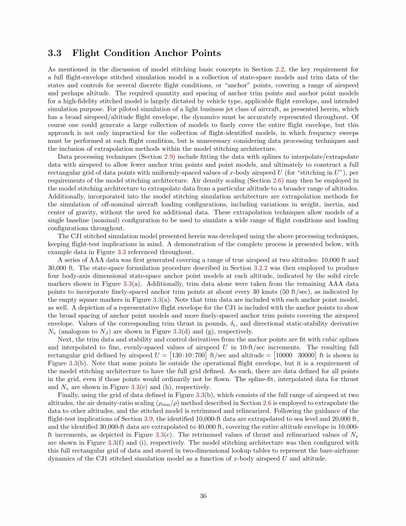
3.3 Flight Condition Anchor Points

As mentioned in the discussion of model stitching basic concepts in Section 2.2, the key requirement fora full flight-envelope stitched simulation model is a collection of state-space models and trim data of thestates and controls for several discrete flight conditions, or “anchor” points, covering a range of airspeedand perhaps altitude. The required quantity and spacing of anchor trim points and anchor point modelsfor a high-fidelity stitched model is largely dictated by vehicle type, applicable flight envelope, and intendedsimulation purpose. For piloted simulation of a light business jet class of aircraft, as presented herein, whichhas a broad airspeed/altitude flight envelope, the dynamics must be accurately represented throughout. Ofcourse one could generate a large collection of models to finely cover the entire flight envelope, but thisapproach is not only impractical for the collection of flight-identified models, in which frequency sweepsmust be performed at each flight condition, but is unnecessary considering data processing techniques andthe inclusion of extrapolation methods within the model stitching architecture.

Data processing techniques (Section 2.9) include fitting the data with splines to interpolate/extrapolatedata with airspeed to allow fewer anchor trim points and point models, and ultimately to construct a fullrectangular grid of data points with uniformly-spaced values of x-body airspeed U (for “stitching in U”), perrequirements of the model stitching architecture. Air density scaling (Section 2.6) may then be employed inthe model stitching architecture to extrapolate data from a particular altitude to a broader range of altitudes.Additionally, incorporated into the model stitching simulation architecture are extrapolation methods forthe simulation of off-nominal aircraft loading configurations, including variations in weight, inertia, andcenter of gravity, without the need for additional data. These extrapolation techniques allow models of asingle baseline (nominal) configuration to be used to simulate a wide range of flight conditions and loadingconfigurations throughout.

The CJ1 stitched simulation model presented herein was developed using the above processing techniques,keeping flight-test implications in mind. A demonstration of the complete process is presented below, withexample data in Figure 3.3 referenced throughout.

A series of AAA data was first generated covering a range of true airspeed at two altitudes: 10,000 ft and30,000 ft. The state-space formulation procedure described in Section 3.2.2 was then employed to producefour body-axis dimensional state-space anchor point models at each altitude, indicated by the solid circlemarkers shown in Figure 3.3(a). Additionally, trim data alone were taken from the remaining AAA datapoints to incorporate finely-spaced anchor trim points at about every 30 knots (50 ft/sec), as indicated bythe empty square markers in Figure 3.3(a). Note that trim data are included with each anchor point model,as well. A depiction of a representative flight envelope for the CJ1 is included with the anchor points to showthe broad spacing of anchor point models and more finely-spaced anchor trim points covering the airspeedenvelope. Values of the corresponding trim thrust in pounds, δt, and directional static-stability derivativeNv (analogous to Nβ) are shown in Figure 3.3(d) and (g), respectively.

Next, the trim data and stability and control derivatives from the anchor points are fit with cubic splinesand interpolated to fine, evenly-spaced values of airspeed U in 10-ft/sec increments. The resulting fullrectangular grid defined by airspeed U =

[130:10:700

]ft/sec and altitude =

[10000 30000

]ft is shown in

Figure 3.3(b). Note that some points lie outside the operational flight envelope, but it is a requirement ofthe model stitching architecture to have the full grid defined. As such, there are data defined for all pointsin the grid, even if those points would ordinarily not be flown. The spline-fit, interpolated data for thrustand Nv are shown in Figure 3.3(e) and (h), respectively.

Finally, using the grid of data defined in Figure 3.3(b), which consists of the full range of airspeed at twoaltitudes, the air density-ratio scaling (ρsim/ρ) method described in Section 2.6 is employed to extrapolate thedata to other altitudes, and the stitched model is retrimmed and relinearized. Following the guidance of theflight-test implications of Section 3.9, the identified 10,000-ft data are extrapolated to sea level and 20,000 ft,and the identified 30,000-ft data are extrapolated to 40,000 ft, covering the entire altitude envelope in 10,000-ft increments, as depicted in Figure 3.3(c). The retrimmed values of thrust and relinearized values of Nvare shown in Figure 3.3(f) and (i), respectively. The model stitching architecture was then configured withthis full rectangular grid of data and stored in two-dimensional lookup tables to represent the bare-airframedynamics of the CJ1 stitched simulation model as a function of x-body airspeed U and altitude.

36

0

10000

20000

30000

40000

Raw DataA

ltitu

de [f

t](a)

Interpolation with Airspeed

(b)

Extrapolation with Altitude

(c)

500

1000

1500

2000

2500

δ t [lb]

(d) (e) (f)

200 400 600 8000

0.01

0.02

0.03

Nv

(g)

200 400 600 800x-body airspeed, U [ft/sec]

(h)

200 400 600 800

(i)

Trim

Model

Anchor Points

Figure 3.3: Spline-fit data and air density-ratio extrapolation to cover entire flight envelope.

3.4 Additional Features

Additional features specific to a light business jet class of aircraft were incorporated into the CJ1 stitchedmodel. Flap effects, simple engine model with the capability to control thrust output from each aircraftengine separately, and drag from deployed landing gear and spoilers are discussed.

3.4.1 Flap Effects

The aerodynamic effects of flaps on trim and bare-airframe dynamics have been integrated into the CJ1stitched model. Scaling and corrections of the values of trim attitude, trim controls, and some secondarystability and control derivatives as a function of flap deflection and airspeed were analyzed from AAA truthmodels configured with two different flap settings. These correction effects were then applied to the baselinepoint models and stored as an additional interpolation dimension in the lookup tables of derivatives and trim.This additional interpolation dimension allows for continuous simulation of various flap settings throughoutthe flight envelope for piloted evaluations.

For the flight conditions analyzed using the AAA CJ1 model, flap deflection considerably affects trimpitch attitude, elevator deflection, and thrust, but has only a minor effect on the stability and controlderivatives [1]. As a result, an adequate simulation of first-order effects for deployed flaps is achieved byusing changes in trim only and retaining the flaps-up stability and control derivatives. Verification of thisapproach in the CJ1 stitched model for flap deflections of 15 and 35 degrees is provided in Section 3.8.

37

3.4.2 Simple Engine Model

A simple engine model has been incorporated into the CJ1 stitched model, which takes input in throttleposition and converts it to engine thrust in pounds, δt. Throttle position (with a range of 0–1) is first scaledby the maximum available engine thrust to convert to commanded thrust, δtcmd

. Maximum and idle thrustvalues are looked-up as functions of altitude and Mach. Finally, the engine response dynamics are modeledby a second-order transfer function with a natural frequency of 3 rad/sec and a damping ratio of 1:

δtδtcmd

=ω2n

s2 + 2ζωns+ ω2n

=9

s2 + 6s+ 9(3.4)

Included in the engine model is the ability to control the thrust output of each of the two enginesseparately. Rather than formulating the state-space models with two thrust control derivative (one foreach engine), a simple moment arm component is introduced in conjunction with total thrust output and issummed with the total moment calculation (see Section 2.4.2). For piloted simulation, this feature allows thepilot to realistically employ each throttle. Asymmetrical thrust could be utilized to simulate a one-engine-outcondition, for example.

3.4.3 Component Drag

Unlike the drag effects due to flaps which are implicitly included (i.e., in Xu) by scheduling trim attitudeand controls with flap deflection, the drag effects due to the deployment of landing gear and spoilers areincorporated in the stitched model through an external force. Each drag component is modeled as anequivalent flat-plate drag area and scaled by dynamic pressure and deployment amount (with a continuousrange of 0–1) to obtain dimensional drag force in pounds. Total drag of all components is summed and inputas an external force vector into the nonlinear equations of motion (see Section 2.4.2).

3.5 Nondimensional Derivatives

The argument can be made that nondimensional stability and control derivatives are relatively constant andremain essentially unchanged over the flight envelope, thus utilizing nondimensional derivatives as opposedto their dimensional counterparts may reduce the required number of point models necessary to formulatea stitched model. Although some nondimensional derivatives are indeed relatively constant as a function ofMach over the flight envelope, there are some key nondimensional derivatives that are significantly affectedby Mach affects. Additionally, some nondimensional derivatives do not collapse with Mach, but rather area function of additional variables including angle of attack and density altitude.

The following demonstration will show that the same number of point models are required if nondimen-sional derivatives are employed. Figure 3.4 shows values of example nondimensional derivatives from theAAA CJ1 model for the full flight-envelope range of airspeed and altitude plotted versus Mach; y-axes arescaled to approximately ±40% of the mean derivative value. Indeed some nondimensional derivatives docollapse nicely, showing a smooth trend as a function of Mach alone. However, even relatively-constantderivatives such as Clp and Cyδr do not collapse to a single value but vary somewhat over the flight envelope;Clp and Cyδr vary by approximately 15% and 25%, respectively, over the flight envelope.

As mentioned, there are key nondimensional derivatives that are significantly affected by Mach effects.Cmα is shown to be nearly constant up to Mach 0.6, at which point the values change by a modest 10%.The values of CDδe , however, begin diverging at Mach 0.5 and result in a 20% change by Mach 0.68.

An extreme result of Mach effect is seen in the “tuck” derivative Cmu , in which the values around Mach0.6 rapidly change sign and also increase in magnitude by approximately 45–65%, depending on altitude.This sudden change in sign must be captured for accurate simulation through the high-subsonic regime.Additionally, the values of the lateral-directional derivative Cnβ are not solely a function of Mach, but alsodepend on angle of attack and density altitude.

These effects necessitate the inclusion of various point models throughout the flight envelope. Recom-mended guidelines for the selection of flight-test points are summarized in Section 3.9, which are applicableto both dimensional and nondimensional derivatives.

38

-0.7

-0.6

-0.5

-0.4

-0.3C

l p

0.15

0.2

0.25

0.3

0.35

Cy δ r

-3.5

-3

-2.5

-2

-1.5

Cm

α

0.006

0.008

0.01

0.012

0.014

CD

δ e

0.1 0.2 0.3 0.4 0.5 0.6 0.7-0.06

-0.04

-0.02

0

0.02

0.04

Cm

u

Mach0.1 0.2 0.3 0.4 0.5 0.6 0.7

0.06

0.07

0.08

0.09

0.1

0.11

Cn β

Mach

0

10000

20000

30000

40000

Altitude [ft]

Figure 3.4: Nondimensional derivative values vs. Mach over flight envelope, AAA CJ1 model.

3.6 Verification of Extrapolation Methods

The model stitching architecture incorporates extrapolation methods which allow simulation of off-nominalaircraft loading configurations, as discussed in Section 2.5. In order to verify the extrapolation methodsused to simulate off-nominal loading configurations in the CJ1 stitched model, a collection of AAA truthmodels were generated covering ranges of airspeed, gross weight, inertia, and fuselage-station and waterlineCG locations. Additionally, the altitude extrapolation method presented in Section 2.6 is employed and theresults are compared to a collection of AAA truth models covering the full flight-envelope altitude range.

A baseline (nominal) configuration of 8500 lb, mid CG was chosen for the AAA anchor point modelsand anchor trim points used in the stitched model for all results presented in this section. The stitchedmodel, configured only with these baseline anchor points, was then retrimmed (using the MATLAB functionfindop [12]) and relinearized (using the MATLAB function linearize [12]) at each off-nominal verificationpoint, with the results verified against the database of AAA truth models.

The results presented in this section verify the accommodation in the model stitching architecture foroff-nominal weight and inertia (Section 2.5.1), CG location (Section 2.5.2), and altitude (Section 2.6) asapplied to the CJ1 fixed-wing aircraft example. Additional verification results are provided in Appendix B.

39

3.6.1 Weight

Variations in the simulation value of gross weight were investigated in the CJ1 stitched model. Note thatweight was varied independently, with values of inertia held constant.

Figure 3.5 shows results of simulating off-nominal values of weight in the CJ1 stitched mode. The stitchedmodel, configured only with anchor point models and trim data of the nominal 8500-lb configuration (solidsymbols), was retrimmed and relinearized for various simulation values of gross weight over a range ofairspeed (dashed lines) and compared with values from the AAA truth models (solid lines). Overall, thereis excellent agreement between the stitched model and the truth data.

An increase in trim angle of attack is needed with an increase in gross weight, as expected, due to greaterlift required to balance the weight. This effect is seen more strongly in the lower-airspeed regime, where agreater change in angle of attack is required to generate the required lift due to lower dynamic pressure. Thestitched model tracks the changes in trim angle of attack nearly perfectly, as compared to the truth data.Similarly, the required trim thrust in pounds δt increases with an increase in gross weight, but effectivelyonly in the low- to mid-speed regime. The stitched model accurately extrapolates the trim thrust requiredfor the range of off-nominal weights, with some disparity in the simulated 6000- and 9750-lb configurationsat the low-speed end of the flight envelope. Pertinent stability derivatives Zq and Yv (analogous to Yβ) agreeperfectly with values from the AAA truth data.

These results verify the capability to extrapolate to off-nominal values of weight using only point modelsand trim data of a nominal weight. See Section B.1 for additional off-nominal weight verification results.

-2

0

2

4

6

8

10

α [d

eg]

100 150 200 250 300 350 400

500

1000

1500

2000

δ t [lb]

Airspeed [kn]

-35

-30

-25

-20

-15

-10

-5

0Z

q

100 150 200 250 300 350 400-0.5

-0.4

-0.3

-0.2

-0.1

0

Yv

Airspeed [kn]

Stitched Model

6000

7250

8500

9750

Truth Weight [lb]Anchor Pt.

increasingweight

Figure 3.5: Verification of off-nominal weight extrapolation.

40

3.6.2 Inertia

Variations in the simulation values of the moments of inertia Ixx, Iyy, and Izz were investigated individuallywithin the CJ1 stitched model. The results are discussed over the succeeding subsections, with an examplefigure for the roll inertia results only; see Section B.2 for the complete set of off-nominal inertia verificationfigures. Note that inertia was varied independently of weight for the results presented herein.

Roll Inertia

Results of simulating off-nominal values of roll inertia Ixx are shown in Figure 3.6. The stitched model,configured with only anchor point models and trim data of the nominal configuration (solid symbols), wasretrimmed and relinearized for various simulation values of roll inertia over a range of airspeed (dashed lines)and compared with values from the AAA truth models (solid lines). There is virtually perfect agreementbetween the stitched model and the truth data.

Trim angle of attack is unaffected by the change in inertia, as expected, and is in agreement with thetruth data. Roll inertia affects the lateral/directional stability and control moment derivatives only, mostnotably Lv, Lp, Lr, Lδa , Lδr , Np, and Nδa . The values of these key lateral/directional moment derivativesare inversely proportional to values of Ixx, as tracked well by the stitched model. In the case of Lδa , forexample, an increase in roll inertia yields a smaller external roll moment for a given aileron input. Lateralstability and control force derivatives, such as Yv, are unaffected by changes in roll inertia. Additionally,trim controls and longitudinal stability and control derivatives are unaffected by changes in roll inertia, aspredicted by the stitched model. See Section B.2.1 for additional off-nominal roll inertia verification results.

-2

0

2

4

6

8

10

α [d

eg]

100 150 200 250 300 350 400-10

-8

-6

-4

-2

0

L p

Airspeed [kn]

0

1

2

3

4

Nδ a

100 150 200 250 300 350 4000

10

20

30

40

50

60

70

L δ a

Airspeed [kn]

Stitched Model

8360

9802

11243

Truth Ixx [slug-ft2]Anchor Pt.

increasingroll inertia


Figure 3.6: Verification of off-nominal inertia extrapolation, roll inertia Ixx.

41

Pitch Inertia

See Section B.2.2 for the off-nominal pitch inertia verification results. In contrast to changes in roll inertia,a change in pitch inertia Iyy affects only the longitudinal moment derivatives, specifically Mu, Mw, Mq,Mδe , and Mδt . The values of the primary pitching moment derivatives are inversely proportional to valuesof Iyy, as captured by the stitched model. With key control derivative Mδe , for example, an increase in pitchinertia yields a smaller external pitch moment for a given elevator input. An equivalent relation is seen in thevalues of the pitch damping derivative Mq. Trim attitude and controls and all lateral/directional stabilityand control derivatives are unaffected by changes in pitch inertia, as expected.

Yaw Inertia

See Section B.2.3 for the off-nominal yaw inertia verification results. A change in yaw inertia Izz has asignificant effect only on the lateral/directional moment derivatives, specifically Nv, Np, Nr, Nδa , Nδr , Lr,and Lδr . The values of these lateral/directional moment derivatives are inversely proportional to valuesof Izz, as captured well by the stitched model. Trim attitude and controls, and longitudinal stability andcontrol derivatives are unaffected by changes in yaw inertia.


Off-nominal simulation values of center of gravity (CG) location were investigated in the CJ1 stitched model.Changes in fuselage-station CG location (x-body axis, positive aft) and waterline CG location (z-body axis,positive up) were investigated. The results are discussed in the succeeding subsections, with an example figurefor the fuselage-station CG results only; see Section B.3 for the complete set of off-nominal CG verificationfigures.

Station CG

Figure 3.7 shows results of simulating off-nominal values of fuselage-station CG location (x-body axis, positiveaft) in the CJ1 stitched model. The stitched model, configured only with anchor point models and trimdata of the nominal mid-CG (244.3 in, or 22.5% MAC) configuration (solid symbols), was retrimmed andrelinearized for simulation values of a forward (240.1 in, or 16.5% MAC) and aft (248.4 in, or 28.5% MAC)fuselage-station CG over a range of airspeed (dashed lines) and compared with values from the AAA truthdata (solid lines). Overall the stitched model agrees nearly perfectly with the truth data.

Trim elevator deflection moves downward (positive direction) as the CG moves aft (higher value of stationCG) due to decreased download required on the tail, while trim angle of attack remains virtually unchangedas gross weight is held constant. In addition, key stability derivative Mw, which is analogous to Mα, decreasesin magnitude, thus indicating decreased static margin, as expected for the aft CG shift. A similar trend isseen in the directional static-stability derivative Nv, which is analogous to Nβ .

This verifies the capability to extrapolate to off-nominal values of CG using only point models of anominal CG. See Section B.3.1 for additional off-nominal fuselage-station CG verification results.

Waterline CG

See Section B.3.2 for the off-nominal waterline CG verification figures. Variations in waterline CG (z-bodyaxis, positive up) over the investigated range yield little change in trim attitude and controls; this includestrim elevator, which contrasts the fuselage-station results. Changes in waterline CG location are most evidentin the roll dynamics, particularly the Lv, Lr, and Lδr derivatives. The longitudinal stability and controlderivatives are essentially unaffected by vertical CG location, with the exception of Mδt ; the pitching momentdue to a change in thrust is affected by the vertical offset distance between the CG and the engines. Withan increase in value of waterline CG (up), the vertical offset between the CG and engines decreases, thusMδt decreases, as confirmed by the data.

42

-15

-10

-5

0

5δ e [d

eg]

100 150 200 250 300 350 400-2

0

2

4

6

8

10

α [d

eg]

Airspeed [kn]

-0.16

-0.14

-0.12

-0.1

-0.08

-0.06

-0.04

-0.02

Mw

100 150 200 250 300 350 4000.005

0.01

0.015

0.02

Nv

Airspeed [kn]

Stitched Model

240.1

244.3

248.4

Truth Station CG [in]Anchor Pt.

aft CG

aft CG

Figure 3.7: Verification of off-nominal CG extrapolation, fuselage station.

3.6.4 Altitude

Simulation of alternate altitudes in the stitched model involves scaling the dimensional stability and controlderivatives and specific aerodynamic trim forces by the air density ratio ρsim/ρ, which is the ratio of airdensity at the simulation altitude to that at the baseline altitude, and retrimming/relinearizing the stitchedmodel (see Section 2.6). Considering flight-test implications, the strategy implemented in this case of theCJ1 model was to perform the extrapolation based on two sets of anchor point models and trim data; one setof data configured at 10,000 ft, and the second set configured at 30,000 ft. The air density-ratio extrapolationwas then performed on each set of data and the results were combined. Specifically, the 10,000-ft data areextrapolated to sea level and 20,000 ft, and the 30,000-ft data are extrapolated to 40,000 ft, covering theentire altitude envelope in 10,000-ft increments. See the discussion of flight-test implications in Section 3.9for more details on this strategy. An alternate technique would be to linearly interpolate between the knownanchor point data to cover the entire altitude range; however, the following demonstration will show theadvantage of air density-ratio scaling for the CJ1 model.

Figure 3.8 compares results of the two abovementioned techniques (air density-ratio scaling and linearinterpolation) applied to data of two 240-knot point models, one at 10,000 ft and the other at 30,000 ft, tocover the full range of altitude. Several additional 240-kn point models were generated for a range of altitudes,which serve as truth data, and the values of example parameters are plotted versus altitude (square symbols).The data at the two anchor altitudes of 10,000 ft and 30,000 ft (circle symbols) are shown connected withsolid lines and extended over the full altitude range, indicating linear interpolation. Conversely, the data atthe two anchor altitudes were also retrimmed and relinearized over the full range of altitude using the air

43

density-ratio scaling technique, as shown by the blue dashed lines for the 10,000-ft data, and by the orangedashed lines for the 30,000-ft data.

-8

-6

-4

-2

0

2

4

δ e [deg

]

400

600

800

1000

1200

1400

1600

1800

δ t [lb]

-35

-30

-25

-20

-15

-10

-5

Mδ e

0

0.5

1

1.5

2

2.5

3

Nδ a

0 10000 20000 30000 40000-20

-15

-10

-5

0

Zq

Altitude [ft] 0 10000 20000 30000 40000

-0.05

-0.04

-0.03

-0.02

-0.01

0

L v

Altitude [ft]

Truth Point

Anchor Altitude

Linear Interpolation

Density Scaling, 10,000-ft model

Density Scaling, 30,000-ft model

Figure 3.8: Altitude density-ratio scaling vs. linear interpolation, 240-kn point models.

For trim elevator deflection δe, control derivative Mδe , and stability derivative Zq, the results generatedby the density-ratio scaling technique nearly perfectly match the values of the truth points over the entirealtitude range. The linear variation resulting from interpolation, however, only somewhat coincides withthe truth values for these parameters, with the largest disparities seen at the limits of the altitude range.Furthermore, nearly identical results are seen between the scaled 10,000-ft and 30,000-ft data, suggestingthat the density-ratio scaling technique could be applied to point models and trim data from a single altitudeto generate accurate data over the full altitude range.

Examining trim thrust δt, control derivativeNδa , and stability derivative Lv, however, there are differencesbetween the 10,000-ft and 30,000-ft density-scaled data. The 10,000-ft scaled data very closely match thetruth data from sea level through 20,000 ft, and begin to diverge through the higher altitudes. On theother hand, the 30,000-ft scaled data very closely match the truth data between 30,000 and 40,000 ft, withlarge disparities seen at the lower altitudes. This result suggests that the extent to which air density-ratio

44

scaling may be accurately applied to the CJ1 stitched model is within approximately ±10,000 ft of an anchoraltitude.

Unlike with δe, Mδe , and Zq, in which the density-ratio scaling technique may be applied to data froma single altitude to generate accurate data over the full altitude range, trim thrust, Nδa , and Lv exhibitmore complex variations with changes in altitude. To accurately cover the full range of altitude for theseparameters, the density-scaled results from the two altitude sets are combined. Specifically, the scaled10,000-ft data are used from sea level through 20,000 ft, and the scaled 30,000-ft data are used from 30,000ft to 40,000 ft, accurately representing the data over the entire altitude range in 10,000-ft increments. Thesedata in 10,000-ft altitude increments can subsequently be used to populate the lookup tables in the stitchedmodel, which was the strategy used in the CJ1 stitched model, as discussed in Section 3.3.

Figure 3.9 shows results of a range of simulation flight altitudes in the CJ1 stitched model. The stitchedmodel, configured only with point models and trim data from the two anchor altitudes of 10,000 and 30,000ft (solid symbols), was retrimmed and relinearized over the full altitude/airspeed flight envelope (dashedlines) using the density-ratio scaling technique and compared with values from the AAA truth models (solidlines). Trim elevator deflection and trim thrust track very well with the AAA truth data. The implicitu-speed derivatives are well preserved over the full flight envelope.

These results verify the accuracy of the air density-ratio scaling technique applied to point models andtrim data at two altitudes for fixed-wing aircraft applications. See Section B.4 for the complete set ofoff-nominal altitude verification results.

-25

-20

-15

-10

-5

0

5

δ e [deg

]

100 150 200 250 300 350 400500

1000

1500

2000

2500

δ t [lb]

Airspeed [kn]

-0.04

-0.03

-0.02

-0.01

0X

u

100 150 200 250 300 350 400-0.25

-0.2

-0.15

-0.1

-0.05

Zu

Airspeed [kn]

Stitched Model

0

10000

20000

30000

40000

Truth Altitude [ft]Anchor Pt.

increasingaltitude

Figure 3.9: Verification of altitude extrapolation.

45

3.7 Dynamic Response Check Cases

Two check cases are presented in this section to verify the dynamic response of the CJ1 stitched model ata particular off-nominal flight condition and configuration as compared to the corresponding truth linearpoint model from AAA. The stitched model, configured only with anchor points as outlined in Section 3.3,was retrimmed and relinearized at each check case condition. Primary longitudinal and lateral/directionalfrequency responses, dimensional stability and control derivative values, modes, and time-history verificationplots are presented and discussed for each check case.

3.7.1 Case 1: Mach 0.3, 5000 ft, Nominal Loading Configuration

This section presents the primary dynamic responses for check case 1: Mach 0.3 (195 KTAS), 5000 ft altitude,and nominal weight and CG configuration. This flight condition is one that is at an altitude and airspeedthat differ from the anchor point models. As such, the stitched model has interpolated between anchor pointsin airspeed and extrapolated in altitude using air density-ratio scaling (see Section 3.6.4). A summary of thesimulation loading configuration values compared to those of the nominal configuration, and the simulationflight condition values compared to the nearest anchor point values are provided in Table 3.1. A summaryof the mode natural frequency and damping results is provided in Table 3.2, and a summary of the valuesof dimensional stability and control derivatives is provided in Table 3.3.

Table 3.1: Simulation loading configuration and flight condition – Case 1

Parameter Simulation Value Nominal/Anchor Value(s) Off-Nominal

Loading ConfigurationWeight [lb] 8500 8500CG [in] 244.3 244.3

Flight ConditionAirspeed [kn] 195 180, 210 XAltitude [ft] 5000 10000 X

Figures 3.10–3.13 show the primary longitudinal frequency responses for check case 1. There is near-perfect agreement between the stitched model and the truth AAA point model. The Short Period mode isperfectly captured by the stitched model, and the Phugoid mode is very closely represented (a close matchin natural frequency but a damping of ζ = 0.049 as compared to ζ = 0.052 for the point model, as shownin Table 3.2). The Phugoid mode can be approximated as 2 (ζωn)P = −Xu from Ref. [11], indicating thatPhugoid natural frequency and damping are proportional to the value of Xu. With essentially equal valuesof Phugoid natural frequency between the stitched model and the truth point model, this slight disparity ofapproximately 6% in Phugoid damping can be attributed to the 6% disparity in values of Xu between theimplicit representation of the stitched model compared to that of the point model, as shown in Table 3.3.

46

-60

-40

-20

0

α/δe [rad/rad]

Mag

nitu

de [d

B]

10-2

10-1

100

101

102

-360

-270

-180

-90

Frequency [rad/sec]

Pha

se [d

eg]

-60

-40

-20

0

α/δe [rad/rad]

Mag

nitu

de [d

B]

10-2

10-1

100

101

102

-360

-270

-180

-90

Frequency [rad/sec]

Pha

se [d

eg]

Point ModelStitched Model

Figure 3.10: Case 1: angle of attack response toelevator input comparison.

-50

0

50

100

Vtas

/δe [ft/sec/rad]

Mag

nitu

de [d

B]

10-2

10-1

100

101

102

-360

-270

-180

-90

0

Frequency [rad/sec]

Pha

se [d

eg]

-50

0

50

100

Vtas

/δe [ft/sec/rad]

Mag

nitu

de [d

B]

10-2

10-1

100

101

102

-360

-270

-180

-90

0

Frequency [rad/sec]

Pha

se [d

eg]


Figure 3.11: Case 1: true airspeed response to ele-vator input comparison.

-40

-20

0

20

40

q/δe [rad/sec/rad]

Mag

nitu

de [d

B]

10-2

10-1

100

101

102

-270

-180

-90

0

Frequency [rad/sec]

Pha

se [d

eg]

-40

-20

0

20

40

q/δe [rad/sec/rad]

Mag

nitu

de [d

B]

10-2

10-1

100

101

102

-270

-180

-90

0

Frequency [rad/sec]

Pha

se [d

eg]


Figure 3.12: Case 1: pitch rate response to elevatorinput comparison.

-40

-20

0

20

40

60

nzstab

/δe [g/rad]

Mag

nitu

de [d

B]

10-2

10-1

100

101

102

-360

-270

-180

-90

0

Frequency [rad/sec]

Pha

se [d

eg]

-40

-20

0

20

40

60

nzstab

/δe [g/rad]

Mag

nitu

de [d

B]

10-2

10-1

100

101

102

-360

-270

-180

-90

0

Frequency [rad/sec]

Pha

se [d

eg]


Figure 3.13: Case 1: normal acceleration responseto elevator input comparison.

Figures 3.14–3.17 show the primary lateral/directional frequency response comparisons for check case 1.There is near-perfect agreement in dynamic responses between the stitched model and the truth AAA pointmodel, as confirmed by the near-perfect agreement of all lateral/directional modes and derivatives.

47

-20

-10

0

10

20

pstab

/δa [rad/sec/rad]

Mag

nitu

de [d

B]

10-2

10-1

100

101

102

-90

0

Frequency [rad/sec]

Pha

se [d

eg]

-20

-10

0

10

20

pstab

/δa [rad/sec/rad]

Mag

nitu

de [d

B]

10-2

10-1

100

101

102

-90

0

Frequency [rad/sec]

Pha

se [d

eg]


Figure 3.14: Case 1: roll rate response to aileroninput comparison.

-100

-50

0

50

β/δa [rad/rad]

Mag

nitu

de [d

B]

10-2

10-1

100

101

102

-360

-270

-180

-90

0

Frequency [rad/sec]

Pha

se [d

eg]

-100

-50

0

50

β/δa [rad/rad]

Mag

nitu

de [d

B]

10-2

10-1

100

101

102

-360

-270

-180

-90

0

Frequency [rad/sec]

Pha

se [d

eg]


Figure 3.15: Case 1: sideslip response to aileron in-put comparison.

-10

0

10

20

30

ny/δ

r [g/rad]

Mag

nitu

de [d

B]

10-2

10-1

100

101

102

-360

-270

-180

-90

Frequency [rad/sec]

Pha

se [d

eg]

-10

0

10

20

30

ny/δ

r [g/rad]

Mag

nitu

de [d

B]

10-2

10-1

100

101

102

-360

-270

-180

-90

Frequency [rad/sec]

Pha

se [d

eg]


Figure 3.16: Case 1: lateral acceleration response torudder input comparison.

-80

-60

-40

-20

0

20

β/δr [rad/rad]

Mag

nitu

de [d

B]

10-2

10-1

100

101

102

-180

-90

0

90

Frequency [rad/sec]

Pha

se [d

eg]

-80

-60

-40

-20

0

20

β/δr [rad/rad]

Mag

nitu

de [d

B]

10-2

10-1

100

101

102

-180

-90

0

90

Frequency [rad/sec]

Pha

se [d

eg]


Figure 3.17: Case 1: sideslip response to rudder in-put comparison.

Summaries of the natural modes and dimensional stability and control derivative values for this checkcase are provided in Tables 3.2 and 3.3, respectively. Overall, there is near-perfect agreement in naturalfrequency and damping of the modes. The only noteworthy discrepancy is that the Phugoid mode in thestitched simulation model is slightly less damped (ζ = 0.049 as compared to ζ = 0.052 of the truth pointmodel), as already mentioned.

Figures 3.18–3.20 show the short- and long-term time-history response comparisons for three separatecontrol input doublets. Figure 3.18 shows the total airspeed Vtot and angle of attack response comparisons fora 5-deg elevator doublet. Angle of attack is nearly perfectly simulated by the stitched model, and excellentagreement is seen in the airspeed response. Figure 3.19 shows the response comparisons of roll rate andsideslip angle for a 5-deg aileron doublet, and Figure 3.20 shows the lateral acceleration and sideslip angleresponse comparisons for a 5-deg rudder doublet, with near-perfect agreement for all lateral/directionalresponses.

48

Table 3.2: Modes – Case 1

Mode Parameter Stitched Model Point Model

Phugoidωn [rad/sec] 0.1379 0.1371ζ 0.0487 0.0515

Short Periodωn [rad/sec] 5.4745 5.4745ζ 0.4597 0.4598

Spiral 1/τ [rad/sec] −0.0004 −0.0004

Dutch Rollωn [rad/sec] 2.1190 2.1189ζ 0.1019 0.1019

Roll Subsidence 1/τ [rad/sec] 4.2035 4.2034

Table 3.3: Stability and Control Derivatives, Body Axes – Case 1

Derivative Stitched Model Point Model

Xu −0.0125 −0.0132Zu −0.1652 −0.1663Mu 0.0028 0.0027Xw 0.0801 0.0800Zw −1.8684 −1.8684Mw −0.0756 −0.0756Xq 0.2169 0.2166Zq −10.9679 −10.9676Mq −3.1661 −3.1670

Yv −0.1971 −0.1971Lv −0.0217 −0.0216Nv 0.0111 0.0111Yp −0.8436 −0.8436Lp −4.0914 −4.0913Np −0.4193 −0.4193Yr 2.2137 2.2137Lr 0.6004 0.6005Nr −0.3463 −0.3463

Xδe −0.0267 −0.0276Zδe −49.3874 −49.4219Mδe −17.5990 −17.5971Xδt 0.0038 0.0038Zδt −0.0002 −0.0002Mδt −0.0001 −0.0001

Lδa 18.0682 18.0666Nδa 1.0515 1.0513Yδr 23.7677 23.7655Lδr 1.7534 1.7530Nδr −4.5688 −4.5684

49

193

194

195

196

197

Vto

t [kn]

0 1 2 3 4 5-4

-2

0

2

4

6

time [sec]

α [d

eg]

0 50 100 150 200 250time [sec]


Figure 3.18: Case 1: short- and long-term time history responses, elevator doublet.

-40

-20

0

20

40

p [d

eg/s

ec]

0 1 2 3 4 5-5

0

5

time [sec]

β [d

eg]

0 5 10 15 20 25 30time [sec]


Figure 3.19: Case 1: short- and long-term time history responses, aileron doublet.

-0.5

0

0.5

n y [g]

0 1 2 3 4 5-20

-10

0

10

20

time [sec]

β [d

eg]

0 5 10 15 20 25 30time [sec]


Figure 3.20: Case 1: short- and long-term time history responses, rudder doublet.

50

3.7.2 Case 2: Mach 0.6, FL350, Heavy Weight, Aft CG

This section presents the primary dynamic responses for check case 2: Mach 0.6 (346 KTAS), Flight Level 350(35,000 ft altitude), heavy weight, aft CG. This check case demonstrates the simulation of a flight conditionand loading configuration to which the stitched model has extrapolated in altitude, weight, and CG, and isinterpolated in airspeed. A summary of the simulation loading configuration values compared to those ofthe nominal configuration, and the simulation flight condition values compared to the nearest anchor pointvalues are provided in Table 3.4. A summary of the mode natural frequency and damping results for thestitched model versus AAA truth point model is presented in Table 3.5, and a summary of the values ofdimensional stability and control derivatives is provided in Table 3.6.



Loading ConfigurationWeight [lb] 9750 8500 XCG [in] 248.4 244.3 X

Flight ConditionAirspeed [kn] 346 330, 360 XAltitude [ft] 35000 30000 X

Overall, the stitched model extrapolates to this flight condition and loading configuration very well. Theonly notable disparity is seen in the Phugoid mode, where the stitched model predicts a natural frequencyof ωn = 0.076 versus ωn = 0.093 for the truth point model, and a damping of ζ = 0.071 as compared toζ = 0.046 for the truth point model, as shown in Table 3.5. The discrepancy in Phugoid frequency anddamping is a result of the mismatch in the values of the speed damping derivatives Xu and Zu between thepoint model and the implicit representation from the stitched model at this flight condition, as shown inTable 3.6.

Figures 3.21–3.24 show the longitudinal frequency responses for check case 2. There is near-perfectagreement in the Short Period mode, but the disparity in the Phugoid frequency and damping is evident inthe low-frequency portion of the responses. The mid- to high-frequency discrepancy seen in the true airspeedresponses of Figure 3.22 is attributed to the mismatch in values of Xw at this flight condition, as tabulatedin Table 3.6.

-60

-40

-20

0

20

α/δe [rad/rad]

Mag

nitu

de [d

B]

10-2

10-1

100

101

102

-360

-270

-180

-90

Frequency [rad/sec]

Pha

se [d

eg]

-60

-40

-20

0

20

α/δe [rad/rad]

Mag

nitu

de [d

B]

10-2

10-1

100

101

102

-360

-270

-180

-90

Frequency [rad/sec]

Pha

se [d

eg]


Figure 3.21: Case 2: angle of attack response toelevator input comparison.

-50

0

50

100

Vtas

/δe [ft/sec/rad]

Mag

nitu

de [d

B]

10-2

10-1

100

101

102

-360

-270

-180

-90

0

Frequency [rad/sec]

Pha

se [d

eg]

-50

0

50

100

Vtas

/δe [ft/sec/rad]

Mag

nitu

de [d

B]

10-2

10-1

100

101

102

-360

-270

-180

-90

0

Frequency [rad/sec]

Pha

se [d

eg]


Figure 3.22: Case 2: true airspeed response to ele-vator input comparison.

51

-40

-20

0

20

q/δe [rad/sec/rad]

Mag

nitu

de [d

B]

10-2

10-1

100

101

102

-270

-180

-90

0

Frequency [rad/sec]

Pha

se [d

eg]

-40

-20

0

20

q/δe [rad/sec/rad]

Mag

nitu

de [d

B]

10-2

10-1

100

101

102

-270

-180

-90

0

Frequency [rad/sec]

Pha

se [d

eg]


Figure 3.23: Case 2: pitch rate response to elevatorinput comparison.

-20

0

20

40

60

nzstab

/δe [g/rad]

Mag

nitu

de [d

B]

10-2

10-1

100

101

102

-360

-270

-180

-90

0

Frequency [rad/sec]

Pha

se [d

eg]

-20

0

20

40

60

nzstab

/δe [g/rad]

Mag

nitu

de [d

B]

10-2

10-1

100

101

102

-360

-270

-180

-90

0

Frequency [rad/sec]

Pha

se [d

eg]


Figure 3.24: Case 2: normal acceleration responseto elevator input comparison.

Figures 3.25–3.28 show the lateral/directional frequency responses for check case 2. There is excellentagreement overall between the stitched model and the point model. The stitched model represents theDutch Roll mode very well (a close match in natural frequency and a damping within approximately 7%),and captures the Roll Subsidence inverse time constant within 1%.

-20

-10

0

10

20

30

pstab

/δa [rad/sec/rad]

Mag

nitu

de [d

B]

10-2

10-1

100

101

102

-90

0

90

Frequency [rad/sec]

Pha

se [d

eg]

-20

-10

0

10

20

30

pstab

/δa [rad/sec/rad]

Mag

nitu

de [d

B]

10-2

10-1

100

101

102

-90

0

90

Frequency [rad/sec]

Pha

se [d

eg]


Figure 3.25: Case 2: roll rate response to aileroninput comparison.

-100

-50

0

50

β/δa [rad/rad]

Mag

nitu

de [d

B]

10-2

10-1

100

101

102

-360

-270

-180

-90

0

Frequency [rad/sec]

Pha

se [d

eg]

-100

-50

0

50

β/δa [rad/rad]

Mag

nitu

de [d

B]

10-2

10-1

100

101

102

-360

-270

-180

-90

0

Frequency [rad/sec]

Pha

se [d

eg]


Figure 3.26: Case 2: sideslip response to aileron in-put comparison.

52

-10

0

10

20

30

ny/δ

r [g/rad]

Mag

nitu

de [d

B]

10-2

10-1

100

101

102

-360

-270

-180

-90

Frequency [rad/sec]

Pha

se [d

eg]

-10

0

10

20

30

ny/δ

r [g/rad]

Mag

nitu

de [d

B]

10-2

10-1

100

101

102

-360

-270

-180

-90

Frequency [rad/sec]

Pha

se [d

eg]


Figure 3.27: Case 2: lateral acceleration response torudder input comparison.

-100

-50

0

50

β/δr [rad/rad]

Mag

nitu

de [d

B]

10-2

10-1

100

101

102

-180

-90

0

90

Frequency [rad/sec]

Pha

se [d

eg]

-100

-50

0

50

β/δr [rad/rad]

Mag

nitu

de [d

B]

10-2

10-1

100

101

102

-180

-90

0

90

Frequency [rad/sec]

Pha

se [d

eg]


Figure 3.28: Case 2: sideslip response to rudder in-put comparison.

The modes for this high-speed cruise check case are summarized in Table 3.5. Overall, there is very goodagreement in natural frequency and damping of all modes. The Phugoid mode is simulated to be at a lowerfrequency (ωn = 0.076 rad/sec versus ωn = 0.093 of the truth point model) and more damped (ζ = 0.071 ascompared to ζ = 0.046 of the truth point model). There is excellent agreement in Short Period, Dutch Roll,and Roll Subsidence modes.

Figures 3.29–3.31 show the short- and long-term time-history response comparisons for three separatecontrol doublets. Figure 3.29 shows the airspeed and angle of attack response comparisons for a 5-degelevator doublet. Angle of attack is nearly perfectly simulated by the stitched model. The airspeed responseis captured relatively well, with the discrepancies in Phugoid frequency and damping as seen in Table 3.5evident in the long-term response comparison. Nevertheless, the differences amount to three cycles in airspeedoscillation observed in 4 minutes as opposed to three and a half cycles seen from the AAA truth point modelover the same time period. This difference in Phugoid frequency is likely unnoticeable to a pilot in simulation.Figure 3.30 shows the response comparisons of roll rate and sideslip angle for a 5-deg aileron doublet. Rollrate is represented very well by the stitched model, and sideslip angle is in excellent agreement. Figure 3.31shows the lateral acceleration and sideslip-angle response comparisons for a 5-deg rudder doublet. There isexcellent agreement in the short- and long-term responses.

53



Phugoidωn [rad/sec] 0.0761 0.0930ζ 0.0712 0.0460

Short Periodωn [rad/sec] 4.6459 4.6369ζ 0.3050 0.3046

Spiral 1/τ [rad/sec] −0.0002 −0.0016


Roll Subsidence 1/τ [rad/sec] 2.3862 2.4021

Table 3.6: Stability and Control Derivatives, Body Axes – Case 2


Xu −0.0095 −0.0068Zu −0.0792 −0.1182Mu 0.0011 0.0017Xw 0.0310 0.0489Zw −1.0497 −1.0548Mw −0.0341 −0.0340Xq 0.0484 0.1226Zq −5.9440 −5.9278Mq −1.7856 −1.7720

Yv −0.1014 −0.1016Lv −0.0127 −0.0123Nv 0.0058 0.0058Yp −0.4663 −0.4663Lp −2.2417 −2.2505Np −0.1758 −0.1968Yr 1.1122 1.1226Lr 0.3351 0.3874Nr −0.1750 −0.1712

Xδe −0.4872 −0.0201Zδe −41.4377 −41.3179Mδe −14.4982 −14.4494Xδt 0.0030 0.0030Zδt −0.0002 −0.0002Mδt −0.0001 −0.0001

Lδa 14.8535 14.8654Nδa 0.6203 0.6410Yδr 18.3189 18.3758Lδr 1.4757 1.4802Nδr −3.4624 −3.4732

54

344

345

346

347

348

Vto

t [kn]

0 1 2 3 4 5-5

0

5

10

time [sec]

α [d

eg]

0 50 100 150 200 250time [sec]


Figure 3.29: Case 2: short- and long-term time history responses, elevator doublet.

-40

-20

0

20

40

p [d

eg/s

ec]

0 1 2 3 4 5-5

0

5

time [sec]

β [d

eg]

0 5 10 15 20 25 30time [sec]


Figure 3.30: Case 2: short- and long-term time history responses, aileron doublet.

-0.5

0

0.5

n y [g]

0 1 2 3 4 5-20

-10

0

10

20

time [sec]

β [d

eg]

0 5 10 15 20 25 30time [sec]


Figure 3.31: Case 2: short- and long-term time history responses, rudder doublet.

55

3.8 Simulation of Alternate Configurations – Flap Setting

Flap effects were incorporated into the CJ1 stitched model for the piloted simulation fidelity assessmentpresented in Ref. [17]. For the piloted simulation, the effects of flaps on both trim and derivatives, asdetermined from AAA, were applied to the baseline point models as a function of flap deflection and airspeed,and stored as an additional interpolation dimension in the lookup tables. This technique provided continuouslook-up of trim and derivatives with deflection of flaps and changes in airspeed for a high-fidelity simulatedapproach to landing. Pilot reaction indicated that trim behavior, and the corresponding migration of thecontrols, however, were the most important effects upon deployment of flaps [17].

Analyses of the variations in trim and derivative values from AAA as a function of flap deflection indicatesignificant changes in trim angle of attack, elevator, and thrust for deployed flaps at a given airspeed.Although some stability and control derivatives also vary with flap deflection, the largest and most significantvariations are seen in trim angle of attack and controls. As such, the initial flap implementation was simplifiedto changes in trim only; the explicit stability and control derivatives remain those of the nominal flaps-upconfiguration. This approach ensures that trim is correct and allows for efficient flight testing.

Considering the implications of collecting flight-test data for the development of a stitched model, thefollowing will demonstrate the modeling of flap deflection as a change in trim only. Figure 3.32 shows resultsof the CJ1 stitched model for simulated flap deflections of 15 and 35 deg. The stitched model, configuredwith trim data and derivatives of the baseline (i.e., flaps-up) configuration, and with trim data only for thetwo flap deflection configurations (solid symbols), was retrimmed and relinearized over a range of airspeed(dashed lines) and compared to values from AAA truth models (solid lines).

-15

-10

-5

0

5

10

δ e [deg

]

100 150 200 250 300500

1000

1500

2000

2500

3000

3500

δ t [lb]

Airspeed [kn]

-10

-5

0

5

10

α [d

eg]

100 150 200 250 300-0.5

-0.4

-0.3

-0.2

-0.1

Zu

Airspeed [kn]

Stitched Model

0

15

35

Truth Flap Setting [deg]Anchor Pt.

Figure 3.32: Alternate configuration verification, flap deflection.

56

For a given airspeed, an increase in flap deflection results in an increase in lift and drag, thus less angleof attack is needed and a greater total thrust is required to maintain trim. The angle of attack and thrustresults from the stitched model track precisely at the anchor trim points, as expected, and overall matchnearly perfectly with values from the off-nominal AAA truth data over a wide range of airspeed.

The values of the implicit speed derivative Zu for all flap settings agree very well with the truth data.This confirms the implicit preservation of Zu in the stitched model by the trim data. Referring to thecomplete set of flap verification figures in Section B.5, some disparities are seen in the values of the implicitspeed derivative Xu for the flaps-down configurations. Note that the values of derivatives Xw and Xδe affectthe values of implicit Xu in the stitched model [see Eq. (2.19)]. From the AAA truth data these derivativesare indeed functions of flap deflection, but are not represented by the trim-only flap implementation in thestitched model. Overall, the modeling of flap deflection as a change in trim only yields good agreementbetween the CJ1 stitched model and the AAA data.

3.9 Flight-Test Implications for Fixed-Wing Aircraft1

A key application of the model stitching architecture is the development of full flight-envelope stitched sim-ulation models from flight-identified point models using system identification methods [1] and associatedflight-test trim data. The extrapolation methods employed in the model stitching architecture permit con-tinuous, full flight-envelope simulation of a full range of aircraft loading configurations using only a smallnumber of point models and trim points. This requirement for a small number of flight-test points directlyreduces the associated flight-test time, cost, and data analysis effort.

This section covers the overall considerations for planning and conducting a flight test involving fixed-wing aircraft for the development of stitched simulation models. Analyses of the sample CJ1 fixed-wing datatrends discussed herein and lessons learned are applied to provide guidance on the spacing and quantityof trim data and point models to be obtained in flight testing. A method is presented for repurposinglongitudinal static stability data, which accurately capture speed derivatives for use in the identified pointmodels, to be combined with the collected trim data in the stitched model. Data processing techniquesare presented, including a technique to account for the natural variance in aircraft weight, CG, and inertiabetween test points due to fuel burn-off. A summary of the overall flight-test recommendations for fixed-wingaircraft is provided in Table 3.7.

3.9.1 Flight-Test Data Collection

Trim Data

The collection of trim test data is accomplished by trimming the aircraft at the desired flight conditionand recording data for a duration of approximately 3–5 seconds. Post-flight processing of the data is doneto determine the trim (average) values of the controls, thrust/power setting, aircraft attitude, and anyadditional states for the particular flight-test point. It is important to know the loading configuration ateach test point, whether it be from accurate onboard estimations of weight and CG or measurements of thefuel load at each point for use with a fuel-burn data sheet post-flight. The trim points are then collectivelybaselined to a nominal loading during data processing, as discussed in Section 3.9.2.

Trim data as a function of airspeed should be obtained via the “trim shot” method, in which powersetting is used to vary airspeed while a level flight path angle is maintained with elevator. It is important tocapture critical inflections in trim curves (e.g., bottom of the power curve, Mach effects, etc.) for accuratesimulation over the full airspeed envelope. Collecting trim data at a speed increment of approximately 30–50 knots over the entire airspeed range should ensure capture of the key trim trends. Prior knowledge ofthe aircraft response behavior over specific airspeed ranges may allow trim to be collected at coarser speedincrements (e.g., every 50 knots) between regions of inflection, necessitating a finer increment for the criticalregions only.

1This section was coauthored with Tom Berger, Aviation Development Directorate (AMRDEC), Moffett Field, CA.

57

Identification Point Models

A frequency-domain-based approach of system identification is suggested, which involves performing pilotedor automated frequency sweeps in the primary axes and processing the flight-test data in CIFER R© [1] toextract state-space models at each flight-test condition. See Ref. [1] for detailed discussions on the collectionof flight-test data, including instrumentation requirements, pilot input methods, and record duration guide-lines. The process of identifying point models is more time consuming than the collection of trim data andinvolves both flight testing and identification analysis efforts, so careful consideration of the required identifi-cation points is critical. As with the collection of trim data, it is important to note the loading configurationat the start of each frequency sweep run, as this information is used during the baselining process.

The analyses of CJ1 stability and control derivative trends over ranges of airspeed (Section 3.6) showthat 4 identified point models are typically sufficient to accurately represent the dynamic response of thefixed-wing aircraft over the entire airspeed range for a particular altitude. This guidance is applicable toboth dimensional and nondimensional derivatives (see Section 3.5). The 4 identification points may beroughly evenly spaced over the entire airspeed range. It is suggested to more-closely space the high-speedidentification points (Mach ≥ 0.5) to accurately capture variations in stability and control derivatives dueto Mach effects.

Longitudinal Static Stability Data

When performing system identification it is common for speed derivatives Xu and Mu to be insensitivedue to lack of frequency response data at frequencies low enough to accurately capture the Phugoid mode.Therefore longitudinal static stability data are collected, which can be used to explicitly calculate thesespeed derivatives [1]. There are various methods for obtaining longitudinal static stability data, but hereinthe “throttle-fixed” method is suggested. In this method, power setting is held constant while the elevator isused to vary airspeed by varying flight path angle (i.e., rate of climb or descent). This is also referred to asthe “stabilized point” method [18]. It is recommended that longitudinal static stability data be collected ateach point for which a model is identified. Collecting the static stability data over a range of approximately−30 to +30 knots relative to each point model flight condition, at an increment of approximately 10 knots,is suggested to accurately capture the Xu and Mu speed derivatives.

While the primary purpose of the longitudinal static stability data is for accurate identification of thespeed derivatives in the point models, these data do provide an additional, and more finely spaced, sourceof trim data around the identification flight conditions. However, these collected data must be processed(i.e., retrimmed) to a level flight path angle using the model stitching architecture to be combined with thecollected trim data, as discussed in Section 3.9.2.

Verification Doublets

Performing piloted doublets at each point for which a model is identified is useful for time-domain verificationof the identified point models and the final stitched model at the anchor point flight conditions. Two doublets,one each for a positive and negative input, in each of the primary axes at each identified point model flightcondition are required for verification.

3.9.2 Data Processing

Baselining

Typically during flight testing there will be a natural variance in aircraft weight between test points dueto fuel burn-off. This change in weight will also affect the inertia values, and will likely affect the CGlocation. Furthermore, fuel transfers during flight (e.g., from external tanks to wing) may also directly affectinertia and CG. As a result, the precise loading configuration will likely vary among the anchor points. Toremove the effects of loading configuration on trim and dynamics, the anchor trim data and identified pointmodels may be baselined to a nominal, or baseline, loading configuration using the model stitching simulationarchitecture. In this process, the integrated extrapolation methods (Section 2.5) are employed to accuratelyretrim the anchor trim points and relinearize the anchor point models to a common loading configuration.These baselined anchor points are then used to construct the final stitched model.

58

When extrapolating for simultaneous changes in inertia and CG it is important to have good estimatedvalues of the actual baseline aircraft loading configuration inertia values at each ID point for the most accurateextrapolation in loading configuration. Inertia estimates may be determined from conceptual design sizingequations [19], or derived from identification data collected a two different CG locations, as proposed inRef. [1].

Longitudinal static stability data collected using the throttle-fixed method, in which rate of climb ordescent is varied, must also be baselined (i.e., retrimmed) to a level flight path angle using the modelstitching architecture to employ the data as additional trim points. This is accomplished by ensuring theclimb or descent is represented by the difference in pitch attitude and angle of attack in the collected flight-test data, then simply retrimming each data point to zero flight path angle. Retrimming to a level flight pathangle necessitates a different trim thrust value, so thrust control derivatives must be identified or explicitlymodeled (see Section A.2.2).

Interpolation

Upon completion of the baselining processing step, the full collection of data is then further processed fordirect use in the model stitching architecture. These processing steps include the fitting of splines to the dataand interpolating the data to a fine grid. Trim data must be formatted as a full rectangular grid, which isa grid constructed from defined axis values for each interpolation dimension, per requirements of the modelstitching architecture interpolation scheme (see Section 2.9.1). Typically, the grid will be defined for a setrange of x-body airspeed U in one dimension and a set range of altitude in the second dimension, coveringthe entire flight envelope. Employing shape-preserving piecewise cubic splines, for example, as discussed inSection 2.9.2, allow the collected data to be interpolated to the defined grid while retaining critical inflectionsin the data.

3.9.3 Aircraft Configurations

The extrapolation methods integrated into the model stitching architecture were shown to very accuratelysimulate loading configurations with off-nominal values of weight, inertia, and CG (see Section 3.6). There-fore, collecting trim data and identification models is necessary using only a nominal (baseline) aircraftloading configuration.

Analyses of the variations in trim and derivative values from AAA as a function of flap deflection indicatesignificant changes in trim angle of attack, elevator deflection, and thrust for deployed flaps at a givenairspeed. Although some stability and control derivatives also vary somewhat with flap deflection, the largestand most significant variations are seen in trim angle of attack and controls. Herein, the flap deflectionimplementation was simplified to changes in trim only. Trim data were included for flap settings of 15and 35 deg, while the stability and control derivatives remain at the nominal (flaps-up) configuration (seeSection 3.8). This approach ensures that flaps-down trim is correct, which is important for piloted simulation[17], and allows for efficient flight testing. Cost permitting, it may be advantageous, however, to directlyidentify the dynamics of a single flaps-down approach configuration using system identification flight testing.

3.9.4 Altitude

Altitude extrapolation for fixed-wing aircraft is accomplished within the model stitching architecture byscaling the dimensional stability and control derivatives and specific aerodynamic trim forces by the airdensity ratio (ρsim/ρ) and retrimming/relinearizing the stitched model, as discussed in Section 2.6. Thisextrapolation method has been shown to be very accurate over ±10,000 ft in altitude change for the CJ1light business jet modeled herein (see Section 3.6.4), and reasonable results were found for greater altitudechanges. Based on this applicable range for altitude extrapolation, point linear models and trim data weregenerated herein at altitudes of 10,000 ft and 30,000 ft; the 10,000-ft data were extrapolated to sea level (0 ft)and 20,000 ft, and the 30,000-ft data were extrapolated to 40,000 ft, which is approximately the operationalservice ceiling of the CJ1. With data at only two altitudes, the entire altitude envelope was effectivelyand accurately covered in 10,000-ft increments by the extrapolation method, as presented and verified inSection 3.6.4.

59

Based on the sample CJ1 results, flight testing at two altitudes is recommended to allow the extrapolationmethod to accurately cover the entire altitude envelope. Therefore, the flight-test data collection processoutlined in Section 3.9.1 should be performed at two altitudes. If flight testing at more than one altitude iscost prohibitive, data collected at a single altitude may be extrapolated to cover the entire flight envelope;however, certain trim and derivative trends may not be precisely represented. Alternatively, trim data alonemay be collected at various altitudes to ensure the capture of key thrust, attitude, and elevator deflectiontrends, whereas just the stability and control derivatives from a single altitude may be extrapolated.

3.9.5 Summary of Recommendations

The overall flight-test recommendations for the development of a fixed-wing aircraft stitched simulation modelare summarized in Table 3.7. These recommendations are based on the analyses of the sample CJ1 stitchedmodel presented herein, and are appropriate for typical business jet and transport aircraft applications.The table provides recommended airspeed increments, quantity of points, and example profile at which toidentify point models and collect trim data. Additionally, recommended altitudes at which to perform thedata collection are provided.

Table 3.7: Summary of flight-test recommendations for development of fixed-wing aircraft stitched models

InterpolationDimension

Parameter ID Point Models Trim Data

AirspeedIncrement [kn] 80–100a 30–50b,c

# of airspeeds 4–6 8–12Example profile [approachd 180 270 330 360] [approache 120 150 180 210 240

270 300 330 360 390]

AltitudeIncrement [ft] 20,000 20,000# of altitudes 1–2f 1–2f

Example profile [10,000 30,000] [10,000 30,000]a Finer increment at high speed (Mach ≥ 0.5) to capture nondimensional derivative variation due to Mach effectsb May need finer increment around critical inflections (e.g., bottom of the power curve)c Can include baselined longitudinal static stability data as fine-increment trim data around identification pointsd Single airspeed; flap effects may be modeled as a change in trim onlye Trim data should be collected for two flap settings over a range of representative airspeedsf Data collection at two altitudes recommended for accurate altitude extrapolation


This chapter presented a state-of-the-art stitched model representative of a Cessna Citation CJ1 developedusing linear point models and trim data derived from the Advanced Aircraft Analysis (AAA) software. AAAwas configured with the CJ1 model included with the software to generate nondimensional stability andcontrol derivatives for point flight conditions. Post-processing was performed on the AAA data to convertthe nondimensional derivatives into dimensional, body-axes derivatives for the formulation of state-spacepoint models. Additional features, including flap effects and a simple engine model, were integrated into theCJ1 stitched model for added realism in piloted simulation.

Verification results of off-nominal extrapolation methods were presented comparing outputs of the stitchedmodel to values from AAA truth data for off-nominal loading configurations and alternate altitudes. Twodynamic response check cases were provided to verify overall simulation fidelity at two discrete flight condi-tions. Lessons learned and implications were considered to provide guidance on future flight testing for thedevelopment of stitched models involving fixed-wing aircraft.

60

4 Rotorcraft Stitched Model: UH-60 Black Hawk

Application of the model stitching simulation architecture for a rotorcraft is demonstrated in this chapterwith a high-order model of the UH-60 Black Hawk helicopter. Rotorcraft present unique modeling challengesdue to their inherent instability, rotor complexity, and large changes in trim and linear stability and controlderivatives over the flight envelope. It is essential to capture key trends and have sufficient modeling detailfor accurate, full flight-envelope piloted simulation.

In addition to demonstrating the use of high-order models in the model stitching simulation architecture,this application also demonstrates the storing and subsequent look-up of data in multiple dimensions, i.e.,stitching in x-body airspeed U and y-body airspeed V , to achieve a more accurate simulation around hover.Stitching in y-body airspeed V results in the implicit representation of the v-speed derivatives (e.g., Yv,Lv, and Nv), analogous to the implicit representation of the u-speed derivatives when stitching in x-bodyairspeed U . “Stitching in U and V ” is implemented for increased accuracy in hover/low-speed conditions,and “stitching in U” only is employed for forward-flight conditions.

Verification results of the off-nominal extrapolation methods covered in Section 2.5 are presented com-paring outputs of the stitched model to values from truth point models for off-nominal configurations andconditions. Two dynamic response check cases are provided to verify overall simulation fidelity at twodiscrete flight conditions and loading configurations. Check case results include comparisons of frequencyresponses, mode natural frequency and damping, stability and control derivative values, and time-historyresponses. Lessons learned and implications are considered to provide guidance on future flight testing forthe development of stitched models from system identification results of rotorcraft.

4.1 Aircraft Model Description

The rotorcraft results herein were generated from high-order simulation models representative of the UH-60ABlack Hawk helicopter. The Black Hawk, pictured in Figure 4.1, is a four-bladed, twin-engine, medium-liftutility helicopter manufactured by Sikorsky Aircraft Corporation. The general characteristics and perfor-mance of the UH-60 are as follows:

• Crew: 2 pilots with 2 crew chiefs• Capacity: 2,640 lb of internal cargo, including 11 troops, or 8,000 lb external load• Rotor diameter: 53 ft 8 in• Length: 64 ft 10 in• Empty weight: 10,624 lb• Loaded weight: 22,000 lb• Powerplant: 2 × General Electric T700-GE-701C turboshaft, 1,890 hp each• Max. cruise speed: 159 kn• Combat radius: 368 mi• Service ceiling: 19,000 ft• Rate of climb: 1,315 ft/min

4.2 State-Space Point Models

4.2.1 Overview of FORECAST Software

The FORECAST [20] mathematical model simulation program was employed to generate state-space modelsof the UH-60. FORECAST implements a set of nonlinear first-order ordinary differential equations fromthe Gen Hel [21] blade-element type nonlinear simulation model, and solves for the coupled rotor/fuselagedynamics to produce a trim solution. The blade motion is for rigid flapping and lead/lag at a hinge; flexible

61

Figure 4.1: UH-60 Black Hawk.

blades are not modeled. Numerical perturbations are used to extract high-order linearized models in state-space form. The linear models are formulated to include the higher-order dynamics of the aircraft (includingrotor flapping and lead/lag motion, inflow, downwash interaction with the fuselage, engine dynamics, andprimary servo dynamics) coupled with the six degrees of freedom of the fuselage.

Although FORECAST is capable of producing high-order linear models with over 50 states, somewhatreduced 26-state models were used herein as an example of highly-accurate yet reasonable high-order models.The models used for the results presented herein do not include primary servo (i.e., actuator) dynamics,engine dynamics, or fuselage/downwash interactions.

4.2.2 State Space Formulation

Twenty-six-state FORECAST models were chosen for the analyses presented herein. These flight-validated,high-order models offer excellent fidelity while employing a reasonable number of states. The 26 statesinclude the 8 fuselage states, plus 18 rotor states: 6 main rotor flapping states, 6 main rotor lead/lag states,4 inflow states (3 main rotor dynamic inflow states and 1 tail rotor inflow state), and 2 main rotor rotationalspeed states. The full 26-state state vector is given as

x =[u v w p q r φ θ β0 β1c β1s β0 β1c β1s

ζ0 ζ1c ζ1s ζ0 ζ1c ζ1s λ0 λ1c λ1s λt ψR Ω]T26

(4.1)

Two subsets of the full state vector, one containing the first 6 fuselage states, and the other containing the18 higher-order rotor states, are referred to as the following:

x6 =[u v w p q r

]T6

(4.2)

xH =[β0 β1c β1s β0 β1c β1s ζ0 ζ1c ζ1s ζ0 ζ1c ζ1s λ0 λ1c λ1s λt ψR Ω

]T18

(4.3)

62

The full high-order state-space representation in x = Ax + Bu form is as follows:

u

v

w

p

q

r

φ

θ

β0

...

Ω

=

Xu Xv Xw Xp Xq −W0 Xr + V0 0 −gcΘ0 Xβ0. . . XΩ

Yu Yv Yw Yp +W0 Yq Yr − U0 gcΦ0cΘ0 −gsΦ0sΘ0 Yβ0. . . YΩ

Zu Zv Zw Zp − V0 Zq + U0 Zr −gsΦ0cΘ0 −gcΦ0sΘ0 Zβ0. . . ZΩ

L′u L′v L′w L′p L′q L′r 0 0 L′β0

. . . L′ΩMu Mv Mw Mp Mq Mr 0 0 Mβ0

. . . MΩ

N ′u N ′v N ′w N ′p N ′q N ′r 0 0 N ′β0

. . . N ′Ω0 0 0 1 sΦ0tΘ0 cΦ0tΘ0 0 0 0 . . . 00 0 0 0 cΦ0 −sΦ0 0 0 0 . . . 0∂β0

∂u∂β0

∂v∂β0

∂w∂β0

∂p∂β0

∂q∂β0

∂r 0 0 ∂β0

∂β0. . . ∂β0

∂Ω

......

......

......

......

.... . .

...∂Ω∂u

∂Ω∂v

∂Ω∂w

∂Ω∂p

∂Ω∂q

∂Ω∂r 0 0 ∂Ω

∂β0. . . ∂Ω

∂Ω

u

v

w

p

q

r

φ

θ

β0

...

Ω

+

Xδlat Xδlon Xδcol Xδped

Yδlat Yδlon Yδcol Yδped

Zδlat Zδlon Zδcol Zδped

L′δlat L′δlon L′δcol L′δped

Mδlat Mδlon Mδcol Mδped

N ′δlat N ′δlon N ′δcol N ′δped

0 0 0 00 0 0 0∂β0

∂δlat

∂β0

∂δlon

∂β0

∂δcol

∂β0

∂δped

......

......

∂Ω∂δlat

∂Ω∂δlon

∂Ω∂δcol

∂Ω∂δped

δlat

δlon

δcol

δped

(4.4)

where sin, cos, and tan have been abbreviated as s, c, and t, respectively. Primed derivatives (′), as definedfollowing Ref. [11] and given in Section A.1.3, account for the influence of the cross-product of inertia Ixz.In the remainder of the text, the primed notation is implied but is generally dropped for convenience.

Stability and control derivatives of the higher-order state equations above are represented in their genericform, but specific nomenclature may be assigned to pertinent derivatives. For example, in the last row we can

recognize that the Ω derivatives are associated with the main rotor toque state equation, e.g., ∂Ω∂Ω = ∂R

∂Ω = RΩ,as used in the state-space model structure for engine response identification in Ref. [1].

The linear A and B matrices of Eq. (4.4) are partitioned into submatrices for use in the model stitchingsimulation architecture following Eq. (2.101). The resultant A66, A6H, AH6, AHH, B6C, and BHC matricesare given as

A66 =

Xu Xv Xw Xp Xq Xr

Yu Yv Yw Yp Yq YrZu Zv Zw Zp Zq ZrL′u L′v L′w L′p L′q L′rMu Mv Mw Mp Mq Mr

N ′u N ′v N ′w N ′p N ′q N ′r

6×6

(4.5)

A6H =

Xβ0. . . XΩ

Yβ0. . . YΩ

Zβ0. . . ZΩ

L′β0

. . . L′ΩMβ0

. . . MΩ

N ′β0

. . . N ′Ω

6×18

(4.6)

63

AH6 =

∂β0

∂u∂β0

∂v∂β0

∂w∂β0

∂p∂β0

∂q∂β0

∂r...

......

......

...∂Ω∂u

∂Ω∂v

∂Ω∂w

∂Ω∂p

∂Ω∂q

∂Ω∂r

18×6

(4.7)

AHH =

∂β0

∂β0. . . ∂β0

∂Ω

.... . .

...∂Ω∂β0

. . . ∂Ω∂Ω

18×18

(4.8)

B6C =

Xδlat Xδlon Xδcol Xδped

Yδlat Yδlon Yδcol Yδped

Zδlat Zδlon Zδcol Zδped

L′δlat L′δlon L′δcol L′δped

Mδlat Mδlon Mδcol Mδped

N ′δlat N ′δlon N ′δcol N ′δped

6×4

(4.9)

BHC =

∂β0

∂δlat

∂β0

∂δlon

∂β0

∂δcol

∂β0

∂δped

......

......

∂Ω∂δlat

∂Ω∂δlon

∂Ω∂δcol

∂Ω∂δped

18×4

(4.10)

It is important to note that in this case the stability derivatives of A66 shown in Eq. (4.5) are not the 6-DOFstability derivatives, rather they are the fuselage-only contributions to the combined multi-body model.

In order to allow meaningful comparisons of stability and control derivative values between those of thelinearized high-order stitched model and those from FORECAST, quasi-steady 6-DOF representations weregenerated by performing model reductions (i.e., state elimination and order reduction using the MATLAB R©

function modred [12]) on the full 26-state models. Henceforth, unless otherwise noted, reference to orcomparison of stability and control derivative values will be those of the quasi-steady 6-DOF representation.

4.3 Hover/Low-Speed Trim Data

Fine-increment trim points around hover are necessary to accurately capture the migration of controls andhelicopter attitude for the simulation of low-speed forward, rearward, sideward, and quartering flight, as wellas the simulation of hovering flight in the presence of winds. These low-speed trim data are included in thestitched model as a function of both x-body airspeed U and y-body airspeed V ; therefore, we employ in thisapplication “stitching in U and V ” in the hover/low-speed regime. As a result, the v-speed derivatives (e.g.,Yv, Lv, and Nv), like the u-speed derivatives, are represented implicitly (see Section 2.8). The spacing andcorresponding gradients between the trim data affect the accuracy of the implicit speed derivatives, whichin turn affect the dynamic response of the stitched model.

Scenarios were investigated to determine recommended spacing and strategies for the collection of trimpoints around hover and the low-speed regime. Sections 4.3.1–4.3.3 present separately the analyses of trimdata for forward/rearward, sideward, and quartering flight. Section 4.3.3 presents also the simulation resultsof hovering flight in the presence of steady winds. In total, the overall recommended trim data points areused for the UH-60 stitched model anchor points, as presented in Section 4.5, and are summarized in theflight-test implications for the development of rotorcraft stitched models in Section 4.9.

4.3.1 Forward/Rearward Flight Trim Data

The effect of the spacing of low-speed forward and rearward trim data points on the accuracy of the implicitu-speed derivatives and the dynamic response at hover is presented. Trim data points as a function of onlyx-body airspeed U at increments of 3, 5, and 10 knots, covering a range of airspeed from −20 kn (rearward)to 20 kn forward airspeed, were investigated in the stitched model. These data points are shown graphicallyin Figure 4.2. Also included and shown graphically in Figure 4.2 are stability and control derivative values

64

-20 -10 0 10 20 30 40

-20

-10

0

10

20

3-kn increment U trim datay-

body

airs

peed

, V [k

n]

(a)

-20 -10 0 10 20 30 40

5-kn increment U trim data

x-body airspeed, U [kn]

(b)

-20 -10 0 10 20 30 40


(c)

Trim Data

Point Model+ Trim Data

Figure 4.2: Forward/rearward flight trim data points at 3-, 5-, and 10-kn x-body airspeed U increments,and point models at hover and 40 kn.

(i.e., point models) only at two points in this low-speed regime: hover and 40 kn, as is typical for rotorcraftidentification [1]. The data were fit with shape-preserving piecewise cubic splines (i.e., MATLAB functioninterp1 with method ‘pchip’ [12]) to interpolate the data to fine 1-kn increment sets over the airspeedrange of the data. The stitched model, configured with the three different trim data sets of varying x-bodyairspeed increment, was then retrimmed and linearized over the −20 to 20 knot airspeed range.

Figure 4.3 shows trim values of the controls, attitude, and longitudinal rotor flapping angle β1c from thestitched model configured for each of the three trim data sets as compared to truth values from FORECAST.Circle, square, and triangle symbols indicate the original data points of the 3-, 5-, and 10-kn sets, respectively,used as anchor points for the spline fits.

3.5

4

4.5

5

δ lon [i

n]

4

4.5

5

5.5

δ lat [i

n]

-20 -10 0 10 204

5

6

7

θ [d

eg]

x-body airspeed, U [kn]-20 -10 0 10 20

-4

-3

-2

-1

φ [d

eg]


1

1.5

2

2.5

3

β 1c [d

eg] Truth

10-kn Increment

5-kn Increment

3-kn Increment

Figure 4.3: Spline-fit forward/rearward flight trim values with various spacing.

65

The truth trim data are captured very well with the 3- and 5-kn spacing over the investigated rear-ward/forward airspeed range. The 10-kn spacing roughly captures the data, but misses subtle inflections inthe trends of pitch attitude θ, longitudinal cyclic stick δlon, and longitudinal rotor flapping angle.

The implicit u-speed derivative values, due to the x-body airspeed U trim data of various spacing, areshown in Figure 4.4 and compared to FORECAST truth data over the same airspeed range of −20 to 20knots. Overall there is excellent agreement of the quasi-steady, implicit u-speed derivative values with thetruth data, with the fine 3-kn-increment data most-closely matching the truth data over the airspeed range,and the 5-kn-increment data also matching well. The 10-kn-increment data once again does not capturesubtle inflections in the derivative values. In addition to the closeness of match of the derivative values overthe airspeed range, the derivative values at the hover point (U = 0) are also affected by the spacing of thedata, due to the gradients between the data to either side of the hover point. As such, the fine 3-kn-incrementdata most-closely match the truth values, and the match slightly degrades as the data become coarser.

-0.1

-0.05

0

0.05

0.1

Xu

-0.1

-0.05

0

0.05

0.1

Yu

-20 -10 0 10 20-0.2

0

0.2

0.4

0.6

Zu


-0.1

-0.05

0

0.05

0.1

L u

-0.01

0

0.01

0.02

Mu

-20 -10 0 10 20-0.01

0

0.01

0.02

Nu


Truth

10-kn Increment

5-kn Increment

3-kn Increment

Figure 4.4: Implicit u-speed derivative values due to forward/rearward flight trim data of various spacing.

To illustrate the effect of the implicit u-speed derivative values at the hover point on the dynamic responseof the stitched model, primary on-axis frequency response comparisons between the high-order stitched modeland the FORECAST truth point model are presented in Figures 4.5 and 4.6. The values of the u-speedderivatives affect the low-frequency coupled Pitch and Roll Phugoid modes, as seen most notably in thelow-frequency portions of the magnitude responses. With coarser spacing of the forward/rearward x-bodyairspeed trim data around hover, the frequency response match below approximately 0.6 rad/sec degrades.

To quantify the effect of the implicit u-speed derivative values on the dynamic response at hover, thenatural frequencies and damping ratios of the Pitch and Roll Phugoid modes are tabulated in Table 4.1, inwhich values of the linearized stitched model for the various trim data increments are compared to valuesfrom the truth FORECAST hover point model. There is good agreement in natural frequencies between thelinearized stitched model and the truth point model; however, the Phugoid damping ratios are most affectedby the spacing of the trim data. The accuracy of the Pitch and Roll Phugoid damping ratio values fromthe stitched model degrades with increasing data coarseness; Pitch Phugoid damping values are within 14%,

66

-60

-40

-20

0

p/δlat

[rad/sec/in]M

agni

tude

[dB

]

10-1

100

101

102

-270

-180

-90

0

90

180

Frequency [rad/sec]

Pha

se [d

eg]

-60

-40

-20

0

p/δlat

[rad/sec/in]M

agni

tude

[dB

]

10-1

100

101

102

-270

-180

-90

0

90

180

Frequency [rad/sec]

Pha

se [d

eg]

Point Model3-kn Increment5-kn Increment10-kn Increment

coarserspacing

Figure 4.5: Roll rate response to lateral cyclic in-put comparison for forward/rearward trim data ofvarious spacing, hover.

-60

-40

-20

0

q/δlon

[rad/sec/in]

Mag

nitu

de [d

B]

10-1

100

101

102

-270

-180

-90

0

Frequency [rad/sec]

Pha

se [d

eg]

-60

-40

-20

0

q/δlon

[rad/sec/in]

Mag

nitu

de [d

B]

10-1

100

101

102

-270

-180

-90

0

Frequency [rad/sec]

Pha

se [d

eg]


coarserspacing

Figure 4.6: Pitch rate response to longitudinal cyclicinput comparison for forward/rearward trim data ofvarious spacing, hover.

Table 4.1: Hover Phugoid modes for forward/rearward trim data of varying x-body airspeed U increment

Mode ParameterStitched Model

Point Model10-kn inc. 5-kn inc. 3-kn inc.

Pitch Phugoidωn [rad/sec] 0.4437 0.4229 0.4291 0.5207ζ −0.3591 −0.3748 −0.4196 −0.4840

Roll Phugoidωn [rad/sec] 0.5556 0.5602 0.5716 0.6524ζ 0.1755 0.2138 0.2388 0.2543

23%, and 26% for the 3-, 5-, and 10-kn-increment data, respectively, and Roll Phugoid damping values arewithin 7%, 16%, and 31% for the 3-, 5-, and 10-kn-increment data, respectively.

Overall, the 3- and 5-kn-increment x-body airspeed U trim data yield satisfactory results, and are recom-mended for the collection of forward/rearward trim data in the hover/low-speed regime. A 5-kn incrementset of forward/rearward trim data is used in the UH-60 stitched model (see Section 4.5).

4.3.2 Sideward Flight Trim Data

Analyses of the spacing of low-speed forward/rearward trim data points on the accuracy of the implicitu-speed derivatives for stitching in U were presented in the previous section. In this section, the effect of thespacing of low-speed sideward flight trim data points on the accuracy of the implicit v-speed derivatives forstitching in V and the dynamic response at hover are presented. Three pure-sideward flight trim data setsof various spacing (3-, 5-, and 7-kn y-body airspeed V increments) were generated in FORECAST covering−15 to 15 knots y-body airspeed V . These data points are shown graphically in Figure 4.7. Stability andcontrol derivative values (i.e., point models) are again included only at hover and 40 kn forward airspeedin this low-speed regime. The data were fit with shape-preserving piecewise cubic splines to interpolate thedata to fine 1-kn increment sets over the full −15 to 15 knot sideward flight range. The stitched model,configured with the three different sideward flight trim data sets, was then retrimmed and linearized for puresideward flight between −15 and 15 knots y-body airspeed V .

Figure 4.8 shows trim values of the controls, bank angle, and lateral rotor flapping angle β1s from thestitched model configured for each of the three sideward trim data sets as compared to truth values fromFORECAST over the sideward airspeed range. Circle, square, and triangle symbols indicate the originaldata points of the 3-, 5-, and 7-kn sets, respectively, used as anchor points for the spline fits. The truth data

67

-20 -10 0 10 20 30 40

-20

-10

0

10

20

3-kn increment V trim datay-

body

airs

peed

, V [k

n]

(a)

-20 -10 0 10 20 30 40

5-kn increment V trim data


(b)

-20 -10 0 10 20 30 40

7-kn increment V trim data

(c)

Trim Data


Figure 4.7: Sideward flight trim data points at 3-, 5-, and 7-kn y-body airspeed V increments, and pointmodels at hover and 40 kn.

are captured very well with the 3- and 5-kn spacing over the displayed sideward airspeed range. The 7-knspacing also captures the trends well, but slightly misses subtle inflections near the extremities of the data,and the fitted spline does not precisely capture the collective δcol data near hover.

Also shown in Figure 4.8 are data labeled “stitching in U only,” which are the results of trimming thestitched model without any y-body airspeed V trim data at all; anchor data points are those shown previouslyin Figure 4.2(b). The stitched model is capable of trimming to the sideward flight points, but without knownsideward trim data the stitched model must rely on the values of the stability and control derivatives atthe hover point to determine a trim solution. As such, the stitched model predicts a linear trend over thesideward airspeed range, missing much of the truth data. This supports the need to capture sideward flighttrim data trends around hover and employ stitching in U and V for accurate hover/low-speed simulation.

4.5

5

5.5

6

δ lat [i

n]

4.5

5

5.5

6

δ col [i

n]

-15 -10 -5 0 5 10 151.5

2

2.5

δ ped [i

n]

y-body airspeed, V [kn]-15 -10 -5 0 5 10 15

-5

-4

-3

-2

-1

φ [d

eg]

y-body airspeed, V [kn]

0.5

1

1.5

β 1s [d

eg]

Truth

7-kn Increment

5-kn Increment

3-kn Increment

Stitching in U only

Figure 4.8: Spline-fit sideward flight trim values with various spacing.

68

The implicit v-speed derivative values, due to the sideward flight trim data of various spacing, arepresented in Figure 4.9 and compared to FORECAST truth data over the same sideward airspeed V rangeof −15 to 15 knots. Overall there is very good agreement between the quasi-steady, implicit v-speed derivativevalues and the truth data, with the fine 3-kn-increment data most-closely matching the truth data over thesideward airspeed range, and the 5-kn-increment data also matching well. The 7-kn-increment results aredegraded, especially in the key stability derivatives Yv and Lv. In addition to the closeness of match of thederivative values over the airspeed range, the derivative values at the hover point (V = 0) are also affectedby the spacing of the data, due to the gradients between the data to either side of the hover point; this ismost clearly seen in the hover point values of Lv. As such, the fine 3-kn-increment data most-closely matchthe truth values, and the match slightly degrades as the data become coarser.

Again, data labeled “stitching in U only” are the results of trimming/linearizing the stitched modelover the sideward airspeed range without any y-body airspeed V trim data; forward airspeed U is the onlyinterpolation dimension. Because the value of U remains at the hover value (U = 0), the looked-up valuesof the v-speed derivatives are, in turn, constantly those of the hover point model over the entire sidewardairspeed range, as seen in the straight dotted lines. These results further support the need for sideward flighttrim data and employing stitching in U and V around hover to accurately preserve the dynamic response insideward flight.

-0.1

-0.05

0

0.05

0.1

Xv

-0.2

-0.15

-0.1

-0.05

0

Yv

-15 -10 -5 0 5 10 15-0.2

-0.1

0

0.1

0.2

Zv


-0.05

-0.04

-0.03

-0.02

-0.01

L v

-0.02

-0.01

0

0.01

0.02

Mv

-15 -10 -5 0 5 10 15-0.02

-0.01

0

0.01

0.02

Nv


Truth

7-kn Increment

5-kn Increment

3-kn Increment

Stitching in U only

Figure 4.9: Implicit v-speed derivative values due to sideward flight trim data of various spacing.

To illustrate the effect of the implicit v-speed derivative values at the hover point on the dynamic responseof the stitched model, primary on-axis frequency response comparisons between the high-order stitched modeland the FORECAST truth point model are presented in Figures 4.10 and 4.11. The values of the v-speedderivatives affect the low-frequency coupled Pitch and Roll Phugoid modes, as seen most notably in thelow-frequency portions of the magnitude responses. With increasing (coarser) spacing of the sideward trimdata, the frequency response match slightly degrades below approximately 0.6 rad/sec.

To quantify the effect of the implicit v-speed derivative values on the dynamic response at hover, thenatural frequency and damping ratio of the Pitch and Roll Phugoid modes are tabulated in Table 4.2, in which

69

-60

-40

-20

0

p/δlat

[rad/sec/in]M

agni

tude

[dB

]

10-1

100

101

102

-270

-180

-90

0

90

180

Frequency [rad/sec]

Pha

se [d

eg]

-60

-40

-20

0

p/δlat

[rad/sec/in]M

agni

tude

[dB

]

10-1

100

101

102

-270

-180

-90

0

90

180

Frequency [rad/sec]

Pha

se [d

eg]


coarserspacing

Figure 4.10: Roll rate response to lateral cyclic in-put comparison for sideward trim data of variousspacing, hover.

-60

-40

-20

0

q/δlon

[rad/sec/in]

Mag

nitu

de [d

B]

10-1

100

101

102

-270

-180

-90

0

Frequency [rad/sec]

Pha

se [d

eg]

-60

-40

-20

0

q/δlon

[rad/sec/in]

Mag

nitu

de [d

B]

10-1

100

101

102

-270

-180

-90

0

Frequency [rad/sec]

Pha

se [d

eg]


coarserspacing

Figure 4.11: Pitch rate response to longitudinalcyclic input comparison for sideward trim data ofvarious spacing, hover.

Table 4.2: Hover Phugoid modes for sideward trim data of varying y-body airspeed V increment

Mode ParameterStitched Model

Point Model7-kn inc. 5-kn inc. 3-kn inc.

Pitch Phugoidωn [rad/sec] 0.4985 0.5043 0.5097 0.5207ζ −0.4317 −0.4345 −0.4444 −0.4840

Roll Phugoidωn [rad/sec] 0.5948 0.6093 0.6223 0.6524ζ 0.2011 0.2191 0.2226 0.2543

values of the linearized stitched model for the various sideward flight trim data increments are compared tothose from the truth FORECAST hover point model. There is very good agreement in natural frequencyand damping between the linearized stitched model with the 3-kn-spaced data and the truth point model;natural frequency and damping are within 3% and 9%, respectively, of the values from the point model forthe Pitch Phugoid mode, and within 5% and 13% for the Roll Phugoid mode. There is also good agreementbetween the stitched model with the 5-kn-spaced data and the truth point model; natural frequency is within4% and damping is within 11% for the Pitch Phugoid mode, and within 7% and 14% for the Roll Phugoidmode. The agreement between the stitched model with the 7-kn-spaced data and the truth point model isacceptable, yet the greatest disparities are seen overall; frequency and damping values within 5% and 11%,respectively, for the Pitch Phugoid mode, and values within 9% and 21% for the Roll Phugoid mode.

Based on these results, the 3- and 5-kn-increment y-body airspeed V trim data yield the most satisfactoryaccuracy, and are therefore recommended for the collection of sideward trim data in the hover/low-speedregime. A 5-kn increment set of sideward trim data is used in the UH-60 stitched model (see Section 4.5).

4.3.3 Quartering Flight Trim Data

Trim data of low-speed quartering flight (i.e., high-sideslip, diagonal flight toward some reference heading)are necessary not only for the simulation of such flight, but also for the simulation of hovering flight in thepresence of quartering winds. Quartering flight at 45 degrees over a range of airspeed was investigated inthe stitched model to verify the accuracy of the implicit v-speed derivatives. Additionally, scenarios of datawith varying radial spacing were investigated to determine recommended radial increments and strategiesfor the collection of low-speed quartering trim points around hover.

70

Constant Flight Direction, Varying Airspeed

Quartering flight (i.e., 45-deg) trim data points at 5-kn airspeed Vtot increments were generated in FORE-CAST covering 0 to 20 knots total airspeed. These data points are shown graphically in Figure 4.12(a).Additionally, forward/sideward-only data points (i.e., no quartering data), shown in Figure 4.12(b), werealso generated for comparison. Stability and control derivative values from point models are again includedonly at hover and 40 kn forward airspeed in both data sets in this low-speed regime. The data were fit withshape-preserving piecewise cubic splines to interpolate the data to a fine 1-kn increment over the 0 to 20knot Vtot quartering flight range. The stitched model, configured with each of the two data sets, was thenretrimmed and linearized for 45-deg quartering flight between hover and 20 knots total airspeed.

-20 -10 0 10 20 30 40

-20

-10

0

10

2045 deg

Quartering trim data

y-bo

dy a

irspe

ed, V

[kn]


(a)

-20 -10 0 10 20 30 40

Forward/sideward only trim data


(b)

Trim Data


Figure 4.12: Quartering and pure forward/sideward flight trim data points at 5-kn airspeed Vtot increments,and point models at hover and 40 kn.

Figure 4.13 shows trim values of the controls, bank angle, and longitudinal rotor flapping angle β1c fromthe stitched model, configured separately with quartering trim data and with forward/sideward only trimdata, as compared to truth values from FORECAST over the 45-deg quartering airspeed range. The circlesymbols indicate the original quartering flight trim data points used as anchor points for the spline fits. Thetruth data are captured very well by the stitched model configured with quartering data over the displayedquartering airspeed range, with the major trends represented. The results of the stitched model configuredwith forward/sideward-only trim data show good agreement near hover, but subtle inflections in the truthdata are not captured, and the agreement degrades at the higher quartering airspeeds. For higher accuracy,especially for applications involving shipboard operations in which quartering flight is common, quarteringdata should be collected.

Data labeled “stitching in U only” are the results of trimming the stitched model without any quarteringor sideward trim data; anchor data points are instead a function of x-body airspeed U only, and are thoseshown previously in Figure 4.2(b). The stitched model is capable of trimming to the quartering flight airspeedpoints without known sideward or quartering trim data, but the stitched model must rely on the values ofthe stability and control derivatives as a function of U only to determine a trim solution. As such, thestitched model predicts a trend that is roughly consistent with the truth data over the quartering airspeedrange, but does not capture inflections.

Figure 4.14 shows the implicit v-speed derivative values obtained from trimming/linearizing the stitchedmodel, configured separately with quartering data and with forward/sideward data only, in 45-deg quar-tering flight from hover through 20 kn total airspeed as compared to the FORECAST truth values. Alsoshown are data labeled “stitching in U only” which are results from the stitched model configured withouty-body airspeed V trim data. The quasi-steady, implicit derivative values from the stitched model config-ured with quartering data track very well with the truth values over the quartering flight airspeed range.Gross inflections in key derivatives Yv, Zv, and Lv are effectively captured. Results of the stitched modelconfigured with forward/sideward-only data roughly capture the truth data near hover, but inflections arenot represented well. Moreover, results of “stitching in U only” follow a linear trend as a function of forwardairspeed U (the cosine component of the 45-deg quartering flight), between the two anchor point models athover and 40 kn, and do not capture any inflections in the truth data. These results support the need tocapture quartering flight trim data trends around hover for accurate simulation of quartering flight.

71

4.5

5

5.5

6

δ lat [i

n]

3.5

4

4.5

5

δ lon [i

n]

0 5 10 15 201.4

1.6

1.8

2

δ ped [i

n]

Total airspeed, Vtot

[kn]0 5 10 15 20

-3

-2

-1

0

1

φ [d

eg]


[kn]

1

1.5

2

2.5β 1c

[deg

] Truth

With Quartering Data

With Forward/Sideward Data Only

Stitching in U only

Figure 4.13: Trim values for 45-deg quartering flight up to 20 kn.

The dynamic response of the high-order stitched model was checked at 10-kn Vtot, 45-deg quartering flight.Figures 4.15 and 4.16 show the frequency response comparisons between the stitched model configured withquartering flight trim data, the stitched model configured with forward/sideward-only trim data, and theFORECAST point model for the 10-kn, 45-deg quartering flight condition. For the stitched model configuredwith quartering flight trim data there is very good agreement in the low-frequency portion of the responses,including the Pitch and Roll Phugoid modes, and excellent agreement over the remainder of the displayedfrequency range. The agreement between the stitched model configured with forward/sideward-only trimdata and the truth point model is degraded in the low-frequency portion of the responses.

The natural modes of the three systems compared in Figures 4.15 and 4.16 are provided in Table 4.3.The stitched model, configured with 45-deg quartering trim data and linearized at the 10-kn, 45-deg quar-tering condition, is in excellent agreement with the truth point model at the same 10-kn, 45-deg quarteringcondition. The low-frequency Pitch and Roll Phugoid modes, which are heavily affected by the implicitspeed derivative values, are in close agreement. Note that the stitched model predicts two real Yaw andHeave poles, whereas the modes are combined into two complex poles in the truth point model. Resultsof the stitched model configured with forward/sideward-only trim data and linearized at the 10-kn, 45-degquartering condition are satisfactory, but show larger discrepancies in the low-frequency Pitch and RollPhugoid modes. These results verify the advantage of collecting and including quartering flight trim data inthe stitched model for improved accuracy in the simulation of quartering flight.

72

-0.05

0

0.05

Xv

-0.12

-0.08

-0.04

0

Yv

0 5 10 15 20-0.2

-0.15

-0.1

-0.05

0

Zv


[kn]

-0.06

-0.05

-0.04

-0.03

L v

0

0.01

0.02

0.03

Mv

0 5 10 15 20-0.01

0

0.01

0.02

Nv


[kn]

Truth

With Quartering Data

With Forward/Sideward Data Only

Stitching in U only

Figure 4.14: Implicit v-speed derivative values for 45-deg quartering flight up to 20 kn.

-60

-40

-20

0

p/δlat

[rad/sec/in]

Mag

nitu

de [d

B]

10-1

100

101

102

-270

-180

-90

0

90

180

Frequency [rad/sec]

Pha

se [d

eg]

-60

-40

-20

0

p/δlat

[rad/sec/in]

Mag

nitu

de [d

B]

10-1

100

101

102

-270

-180

-90

0

90

180

Frequency [rad/sec]

Pha

se [d

eg]

Point ModelStitched Model w/ Quartering DataStitched Model w/ Fwd/Sideward Data Only

Figure 4.15: Roll rate response to lateral cyclic inputfor 10-kn, 45-deg quartering flight.

-80

-60

-40

-20

0

q/δlon

[rad/sec/in]

Mag

nitu

de [d

B]

10-1

100

101

102

-270

-180

-90

0

Frequency [rad/sec]

Pha

se [d

eg]

-80

-60

-40

-20

0

q/δlon

[rad/sec/in]

Mag

nitu

de [d

B]

10-1

100

101

102

-270

-180

-90

0

Frequency [rad/sec]

Pha

se [d

eg]

Point ModelStitched Model w/ Quartering DataStitched Model w/ Fwd/Sideward Data Only

Figure 4.16: Pitch rate response to longitudinalcyclic input for 10-kn, 45-deg quartering flight.

73

Table 4.3: Modes – 10-kn, 45-deg quartering flight

Mode ParameterStitched Model Stitched Model

Point Modelwith fwd/sideward with quarteringdata only data

Yaw/Heaveωn [rad/sec] 0.2273/0.2681 0.2143/0.2663 0.2262ζ 1.0000/1.0000 1.0000/1.0000 0.8668

Pitch Phugoidωn [rad/sec] 0.4758 0.5496 0.6252ζ −0.3314 −0.4014 −0.4012

Roll Phugoidωn [rad/sec] 0.6799 0.7491 0.7751ζ 0.1215 0.1268 0.1443

Pitch Aperiodic 1/τ [rad/sec] 1.1934 1.2971 1.5352

Collective Lead/Lagωn [rad/sec] 2.4455 2.4445 2.5040ζ 0.8601 0.8601 0.8752

Rotor RPM 1/τ [rad/sec] 3.8432 3.8453 3.1485

Roll Aperiodic 1/τ [rad/sec] 4.6227 4.6224 4.3797

Regressive Flapωn [rad/sec] 6.3264 6.3249 6.2485ζ 0.6729 0.6726 0.6440

Constant Inflow 1/τ [rad/sec] 11.3716 11.3701 11.3475

Regressive Lead/Lagωn [rad/sec] 20.3266 20.3258 21.3182ζ 0.2570 0.2569 0.2830

1st Harmonic Inflowωn [rad/sec] 22.2268 22.2255 21.7088ζ 0.9031 0.9032 0.8929

Collective Flapωn [rad/sec] 27.1492 27.1491 27.1355ζ 0.3491 0.3491 0.3478

Progressive Lead/Lagωn [rad/sec] 37.8272 37.8278 37.3950ζ 0.2043 0.2043 0.2404

Tail Rotor Inflow 1/τ [rad/sec] 38.8634 38.8615 43.5981

Progressive Flapωn [rad/sec] 48.7096 48.7090 48.7416ζ 0.0987 0.0987 0.0961

74

Constant Airspeed, Varying Wind Direction

Hovering flight in the presence of steady winds is demonstrated for the UH-60 stitched model by trimmingthe model in a position-held/heading-held hover with a 10-kn wind of varying direction through a complete360 degrees. These analyses employ the steady wind simulation element described in Section 2.4.1. Thestitched model was configured with three separate trim data sets with radial increments of 30 deg, 45 deg,and 90 deg (i.e., no quartering data), all at 5-kn total airspeed Vtot increments, as depicted in Figure 4.17.The 10-kn wind magnitude is also depicted. Stability and control derivative values (i.e., point models) areagain included only at hover and 40 kn forward airspeed.

-20 -10 0 10 20 30 40

-20

-10

0

10

20

0

30

6090

30-deg radial increment trim data

y-bo

dy a

irspe

ed, V

[kn]

(a)

-20 -10 0 10 20 30 40

0

45

90



(b)

-20 -10 0 10 20 30 40

0

90


(c)

Trim Data


Figure 4.17: Trim data points at 30-, 45-, and 90-deg radial increments, with 10-kn magnitude indicated,and point models at hover and 40 kn.

Figure 4.18 presents the results of trimming the stitched model in hover with the presence of a steady 10-kn wind of varying direction. The wind vector was rotated in direction through 360 degrees as the stitchedmodel held the aircraft’s position and Northerly (0-deg) heading. The mapping of the trim cyclic stickposition for all wind directions is shown in lateral (δlat) and longitudinal (δlon, positive aft) components,with winds from the cardinal directions of 0, 90, 180, and 270 deg indicated. The trim values of the remainingtwo controls, collective stick δcol and pedals δped, as well as the trim aircraft bank angle φ and pitch angle θare plotted against wind direction in degrees. Note that indicated wind direction is from a specified heading,and is analogous to flight toward that heading.

The stitched model configured with quartering trim data (i.e., 30- and 45-deg radial increment data)tracks very well with the FORECAST truth data throughout the entire wind rotation. Although the trimresults of the stitched model configured without quartering data (i.e., the 90-deg radial increment data)capture the gross trends in δcol, δped, and pitch angle over the wind direction range, subtle inflections aremissed, most noticeably in the bank angle trend. Furthermore, there are disparities in the mapping of trimcyclic stick position from the stitched model configured with the 90-deg radial data, including discrepanciesin the shape and magnitude of the mapping between 0 and 180 deg, and a reversal of the trends between 180deg and 270 deg. These results support the need for radial trim data for the accurate simulation of hoveringflight in the presence of quartering winds. The 45-deg radial increment data set produces results that arevery close to those of the 30-deg radial increment set, and capture all critical inflections in the truth data.

Based on these and previous results, radial trim data every 45 degrees, with 5-kn Vtot spacing, is rec-ommended for accurate simulation in low-speed forward, rearward, sideward, and quartering flight, as wellas accurate simulation of hover/low-speed flight in the presence of winds. These trim data points are usedto configure the hover/low-speed flight conditions of the UH-60 stitched model, as presented in Section 4.5,and are recommended in flight testing for the development of rotorcraft stitched models (see Section 4.9).

75

4.7 4.8 4.9 5 5.1 5.2 5.3 5.4 5.5 5.6 5.7

4.1

4.2

4.3

4.4

4.5

4.6

4.7

4.8

4.9

δlat

[in]

δ lon [i

n]

0

90

180

270

4.9

5

5.1

5.2

δ col [i

n]

1.6

1.8

2

2.2

δ ped [i

n]

0 45 90 135 180 225 270 315 360-4

-3

-2

-1

φ [d

eg]

Wind direction [deg]0 45 90 135 180 225 270 315 360

4

5

6

7

θ [d

eg]

Wind direction [deg]

Wind Direction [deg]

Truth

30-deg Radial Increment



Figure 4.18: Stitched model trim results of position-held/heading-held hovering flight in the presence of arotating 10-knot wind through 360 degrees.

76

4.4 Forward-Flight Trim Data

In the forward-flight regime of the UH-60 stitched model, “stitching in U” alone is applied, necessitating thecollection of forward-flight trim data as a function of x-body airspeed U only. Analogous to the hover/low-speed trim data analyses presented in Section 4.3, the effects of the spacing of forward-flight trim datapoints on the accuracy of the implicit u-speed derivatives and the dynamic responses at the forward-flightidentification points are presented in this section.

Trim data points as a function of x-body airspeed U at increments of 10 and 20 knots, covering a rangeof airspeed from 20 kn to 160 kn, were investigated in the stitched model. These data points are showngraphically in Figure 4.19. Also included and shown graphically in Figure 4.19 are point models at thefollowing airspeeds in this forward-flight regime: 40, 80, and 120 kn. The trim data were fit with shape-preserving piecewise cubic splines (i.e., MATLAB function interp1 with method ‘pchip’ [12]) to interpolatethe data to fine 1-kn increment sets over the airspeed range of the data. The stitched model, configuredwith the two different trim data sets of 10- and 20-kn x-body airspeed increment, was then retrimmed andlinearized over the 20–160 knot airspeed range.

Figure 4.20 shows trim values of the controls, attitude, and longitudinal rotor flapping angle β1c fromthe stitched model configured for each of the trim data sets as compared to truth values from FORECAST.Square and triangle symbols indicate the original data points of the 10- and 20-kn sets, respectively, used asanchor points for the spline fits. The truth trim data from FORECAST are nearly-perfectly captured withthe 10-kn spacing over the investigated forward-flight airspeed range. The 20-kn spacing captures the dataabove 80 kn very well, but somewhat misses subtle inflections in the trends of pitch attitude θ, longitudinalcyclic stick δlon, and longitudinal rotor flapping angle up to 80kn.

The implicit u-speed derivative values, due to the x-body airspeed U trim data of different spacing, areshown in Figure 4.21 and compared to FORECAST truth data over the same airspeed range of 20–160 knots.Overall there is very good agreement between the quasi-steady, implicit u-speed derivative values and thetruth data, with the 10-kn-increment data most-closely matching the truth data over the airspeed range.The 20-kn-increment data also match well, but show a slightly degraded agreement up through 80 kn andin regions of subtle inflection. Additionally, the derivative values at the point model airspeeds of 40, 80 and120 kn are affected by the spacing of the data, due to the gradients between the data to either side of eachpoint model. In general, the 10-kn-increment data most-closely match the truth values at the identificationpoint airspeeds.

To quantify the effects of the implicit u-speed derivative values on the dynamic response at each identi-fication point, the inverse time constant or natural frequency and damping ratio values of the low-frequencymodes at 40, 80, and 120 kn are tabulated in Table 4.4, in which values of the linearized stitched modelfor the 10- and 20-kn trim data increment sets are compared to values from the truth FORECAST pointmodel at each of the three airspeeds. The corresponding primary on-axis roll and pitch frequency responsecomparisons between the high-order stitched model and the truth point model at 40, 80, and 120 kn arepresented in Figures 4.22–4.27. The values of the u-speed derivatives affect the low-frequency dynamics, as

20 40 60 80 100 120 140 160

-20

-10

0

10

20


y-bo

dy a

irspe

ed, V

[kn]


(a)

20 40 60 80 100 120 140 160



(b)

Trim Data


Figure 4.19: Forward-flight trim data points at 10- and 20-kn x-body airspeed U increments, and pointmodels at 40, 80, and 120 kn.

77

3

3.5

4

4.5

5

5.5

δ lon [i

n]

4

4.5

5

5.5

6

6.5

δ lat [i

n]

20 40 60 80 100 120 140 160-6

-3

0

3

6

θ [d

eg]

x-body airspeed, U [kn]20 40 60 80 100 120 140 160

-6

-3

0

3

6

φ [d

eg]


-2

0

2

4

β 1c [d

eg]

Truth

20-kn Increment

10-kn Increment

Figure 4.20: Spline-fit forward-flight trim values with 10- and 20-kn spacing.

seen in the frequency responses below approximately 0.5 rad/sec. The largest differences between results ofthe 10- and 20-kn increment trim data sets are seen for the 40-kn point model, with the 10-kn-incrementdata more-closely matching the truth modes. The 10-kn-increment data produce somewhat better resultsfor the 80-kn point model, and acceptable results are seen from both sets of data for the 120-kn point.

Overall, the 10-kn-increment x-body airspeed U trim data track very well with the FORECAST truthdata through 80 kn, and yield excellent dynamic response results at the 40- and 80-kn point models. The20-kn-increment trim data have satisfactory agreement with the truth data above 80 kn, and the dynamicresponse at 120 kn is captured well by both 10- and 20-kn increment data sets. Therefore, for the collectionof forward-flight trim data for use in the stitched model, a 10-kn x-body airspeed U spacing is recommendedfrom 20 kn through 80 kn, and thereafter a 20-kn spacing is satisfactory.

In total, the overall recommended hover/low-speed (Section 4.3) and forward-flight trim data points areused for the UH-60 stitched model anchor points, as presented in Section 4.5. These recommendations are alsosummarized in the flight-test implications for the development of rotorcraft stitched models in Section 4.9.

78

-0.08

-0.06

-0.04

-0.02

0

Xu

-0.04

-0.02

0

0.02

0.04

Yu

20 40 60 80 100 120 140 160-0.3

-0.2

-0.1

0

0.1

Zu


-0.02

-0.01

0

0.01

0.02

L u

-0.02

-0.01

0

0.01

0.02

Mu

20 40 60 80 100 120 140 160-0.02

-0.01

0

0.01

0.02

Nu


Truth

20-kn Increment

10-kn Increment

Figure 4.21: Implicit u-speed derivative values due to forward-flight trim data of 10- and 20-kn spacing.

Table 4.4: Low-frequency modes at 40, 80, and 120 kn for forward-flight trim data of 10- and 20-kn x-bodyairspeed U increments

ID Point Mode ParameterStitched Model

Point Model20-kn inc. 10-kn inc.

40 kn

Roll 1/τ [rad/sec] 0.2495 0.2328 0.1981

Pitch Phugoidωn [rad/sec] 0.3060 0.3613 0.4387ζ 0.4047 0.4694 0.5552

Pitch 1/τ [rad/sec] −0.3357 −0.3958 −0.4795

80 kn

Roll 1/τ [rad/sec] 0.1905 0.1870 0.1809


Pitch 1/τ [rad/sec] −0.4314 −0.4482 −0.4532

120 kn

Roll 1/τ [rad/sec] 0.2174 0.2291 0.2538


Pitch 1/τ [rad/sec] −0.4181 −0.4101 −0.3933

79

-80

-60

-40

-20

0

20

p/δlat

[rad/sec/in]M

agni

tude

[dB

]

10-1

100

101

102

-270

-180

-90

0

90

180

Frequency [rad/sec]

Pha

se [d

eg]

-80

-60

-40

-20

0

20

p/δlat

[rad/sec/in]M

agni

tude

[dB

]

10-1

100

101

102

-270

-180

-90

0

90

180

Frequency [rad/sec]

Pha

se [d

eg]

Point Model10-kn Increment20-kn Increment

Figure 4.22: Roll rate response to lateral cyclicinput comparison for forward-flight trim dataof 10- and 20-kn spacing, 40 kn.

-80

-60

-40

-20

0

20

q/δlon

[rad/sec/in]

Mag

nitu

de [d

B]

10-1

100

101

102

-360

-270

-180

-90

0

90

Frequency [rad/sec]

Pha

se [d

eg]

-80

-60

-40

-20

0

20

q/δlon

[rad/sec/in]

Mag

nitu

de [d

B]

10-1

100

101

102

-360

-270

-180

-90

0

90

Frequency [rad/sec]

Pha

se [d

eg]


coarserspacing

Figure 4.23: Pitch rate response to longitudi-nal cyclic input comparison for forward-flighttrim data of 10- and 20-kn spacing, 40 kn.

-80

-60

-40

-20

0

20

p/δlat

[rad/sec/in]

Mag

nitu

de [d

B]

10-1

100

101

102

-270

-180

-90

0

90

180

Frequency [rad/sec]

Pha

se [d

eg]

-80

-60

-40

-20

0

20

p/δlat

[rad/sec/in]

Mag

nitu

de [d

B]

10-1

100

101

102

-270

-180

-90

0

90

180

Frequency [rad/sec]

Pha

se [d

eg]



-80

-60

-40

-20

0

20

q/δlon

[rad/sec/in]

Mag

nitu

de [d

B]

10-1

100

101

102

-270

-180

-90

0

90

180

Frequency [rad/sec]

Pha

se [d

eg]

-80

-60

-40

-20

0

20

q/δlon

[rad/sec/in]

Mag

nitu

de [d

B]

10-1

100

101

102

-270

-180

-90

0

90

180

Frequency [rad/sec]

Pha

se [d

eg]



-80

-60

-40

-20

0

20

p/δlat

[rad/sec/in]

Mag

nitu

de [d

B]

10-1

100

101

102

-270

-180

-90

0

90

180

Frequency [rad/sec]

Pha

se [d

eg]

-80

-60

-40

-20

0

20

p/δlat

[rad/sec/in]

Mag

nitu

de [d

B]

10-1

100

101

102

-270

-180

-90

0

90

180

Frequency [rad/sec]

Pha

se [d

eg]



-80

-60

-40

-20

0

20

q/δlon

[rad/sec/in]

Mag

nitu

de [d

B]

10-1

100

101

102

-360

-270

-180

-90

0

90

Frequency [rad/sec]

Pha

se [d

eg]

-80

-60

-40

-20

0

20

q/δlon

[rad/sec/in]

Mag

nitu

de [d

B]

10-1

100

101

102

-360

-270

-180

-90

0

90

Frequency [rad/sec]

Pha

se [d

eg]



80

4.5 Flight Condition Anchor Points

A series of linear point models and a collection of trim data were generated in FORECAST to be used asanchor points in the UH-60 stitched model. Naturally, a very large collection of point models and trimdata could be used in the stitched model; however, based on the findings presented in Sections 4.3 and 4.4,flight conditions for the point models and trim points were selected to allow the accurate simulation ofthe dynamic response of the helicopter over the airspeed envelope while considering practical flight-testimplications. Thus, four state-space point models (with corresponding trim data) of the following airspeedsare included in the stitched model: hover, 40, 80, and 120 knots.

Fine-increment trim points around hover are necessary to accurately capture the migration of controlsand helicopter attitude for the simulation of low-speed forward, rearward, sideward, and quartering flight,as well as the simulation of hovering flight in the presence of winds. These hover/low-speed trim data areincluded in the stitched model as a function of both x-body airspeed U and y-body airspeed V ; therefore,“stitching in U and V ” is applied in the hover/low-speed regime. This results in the implicit representationof the v-speed derivatives (e.g., Yv and Lv) in addition to the implicit u-speed derivatives. Forward-flighttrim data are included in the stitched model as a function of x-body airspeed U alone; therefore, “stitchingin U” is applied in the forward-flight regime.

Based on the analyses presented in Section 4.3.1, low-speed forward and rearward flight trim data withx-body airspeed U increments of 5 knots were found to produce implicit u-speed derivative values in closeagreement with those from FORECAST truth data at hover and over the investigated airspeed range.Similarly, based on the analyses presented in Section 4.3.2, sideward flight trim data with y-body airspeed Vincrements of 5 knots were found to produce implicit v-speed derivative values in close agreement with thosefrom truth data at hover and over the sideward flight airspeed range. Additionally, per analyses presentedin Section 4.3.3, 45-deg radial increment quartering flight trim points, with total airspeed increments of 5knots, were also included to adequately cover the entire hover/low-speed flight regime, and to allow accuratesimulation of low-speed flight in the presence of winds. This 5-kn spacing was therefore employed hereinfor the selection of forward, rearward, sideward, and quartering trim data points for the UH-60 stitchedmodel around hover. At forward airspeeds above 20 knots, trim points are included in the stitched modelwith a 10-kn spacing up to 80 knots and a coarser 20-kn spacing to high speed to effectively capture criticalinflections in forward-flight trim controls and attitude, as presented in Section 4.4.

The flight conditions of the four state-space point models and all trim points included in the UH-60stitched model are illustrated in Figure 4.28 on a U ,V airspeed grid. Units are displayed in ft/sec and knots.The hover/low-speed (stitching in U and V ) and forward-flight (stitching in U only) regimes are denoted.

-50 0 50 100 150 200 250

-40

-30

-20

-10

0

10

20

30

40

U and V U onlystitching in stitching in


y-bo

dy a

irspe

ed, V

[ft/s

ec]

-20 0 20 40 60 80 100 120 140x-body airspeed, U [kn]

-20

-15

-10

-5

0

5

10

15

20

y-bo

dy a

irspe

ed, V

[kn]

Trim DataPoint Model + Trim Data

Figure 4.28: U ,V airspeed points for anchor trim data and point models included in the stitched model.

81

Two-dimensional interpolation of the hover/low-speed trim data was utilized to construct a full rectan-gular grid of data with uniformly-spaced x-body airspeed U in one dimension and uniformly-spaced y-bodyairspeed V in the second dimension, per requirements of the model stitching architecture interpolationscheme (see Section 2.9.1). The 2-D interpolation of the data was performed using the MATLAB functiongriddata with method ‘v4’, which interpolates a scattered data set over a uniform grid using biharmonicspline interpolation [12]. Specifically, the hover/low-speed rectangular grid is defined by a uniform incrementof 2 ft/sec (approximately 1.2 kn) in both U and V dimensions, covering −40 to 80 ft/sec (−24 to 47 kn)x-body airspeed U , and −40 to 40 ft/sec (−24 to 24 kn) y-body airspeed V .

Sample interpolated data are displayed in Figure 4.29 as 3-D mesh surface plots, showing the interpolatedvalues of trim control positions versus x-body airspeed U and y-body airspeed V over the defined rectangulargrid. Values at the anchor trim points, shown previously in Figure 4.28, are depicted by blue spheres. Theinterpolated mesh data are smooth and precisely capture critical inflections in the anchor trim data.

-40 -20 0 20 40 60 80-40

-200

2040

3

4

5

6

U [ft/sec]V [ft/sec]

δ lat [i

n]

-40 -20 0 20 40 60 80-40

-200

2040

3

4

5

6


δ lon [i

n]

-40 -20 0 20 40 60 80-40

-200

2040

2

3

4

5


δ col [i

n]

-40 -20 0 20 40 60 80-40

-200

2040

1

2

3

4


δ ped [i

n]

Figure 4.29: Two-dimensional interpolation of trim control values to U ,V airspeed full rectangular grid –hover/low-speed regime.

4.6 Verification of Extrapolation Methods

Ranges of airspeed, gross weight, inertia, and CG location were investigated in the UH-60 stitched model inorder to verify the off-nominal extrapolation methods used. A baseline configuration of 16,000 lb, mid CGwas chosen for all FORECAST point models used in the stitched model. The stitched model was retrimmed(using the MATLAB function findop [12]) and relinearized (using the MATLAB function linearize [12])at each verification point, with the results verified against a large database of off-nominal truth FORECASTpoint models. The results verify the built-in accommodation in the model stitching architecture for simulatingoff-nominal values of weight and inertia (Section 2.5.1) and CG location (Section 2.5.2).

82

Variations in altitude were also investigated. Due to the complexity of the rotor system, many stabilityand control derivatives do not scale linearly with air density, so utilizing the fixed-wing altitude extrapolationmethod (see Section 2.6) for a rotorcraft application does not fully predict results for alternate altitudes.Rather, it has been shown herein that linearly interpolating between point models and trim data at differentaltitudes yields very good results for rotorcraft.

For all comparisons of stability and control derivative values presented herein for the rotorcraft example,the full 26-state FORECAST truth models and high-order stitched model were first reduced to quasi-steady6-DOF models. Quasi-steady derivative values are shown for meaningful comparisons and interpretation ofthe stability and control derivatives. Additional off-nominal verification results are provided in Appendix C.

4.6.1 Weight

The method for off-nominal weight extrapolation incorporated in the model stitching simulation architecture,as presented in Section 2.5.1, was utilized on the UH-60 stitched model. Key results of simulating off-nominalgross weights are shown in Figure 4.30. The stitched model, configured only with anchor point modelsand trim data of the nominal 16,000-lb configuration (solid symbols), was retrimmed and relinearized forthree simulation values of gross weight over the full range of airspeed (dashed lines) and compared withFORECAST truth data (solid lines). Overall there is excellent agreement between the values from thestitched model and the truth data.

A change in gross weight mainly affects trim collective δcol around hover and low speed, and has anoticeable effect on trim pitch attitude in the mid- to high-speed range, which are both captured nearlyperfectly by the stitched model. The corresponding longitudinal cyclic stick position δlon (positive aft),affected mainly by trim pitch attitude, is predicted very well by the stitched model. Significant shiftsof the primary heave-axis control derivative Zδcol values are seen with change in weight, where a heavierweight results in a smaller vertical net force for a given collective input, and thus a derivative value ofsmaller magnitude (z-axis positive down). This effect is represented very well by the stitched model; valuesover the airspeed range for the anchor weight configuration are in good agreement, and the values fromretrimming/relinearizing the stitched model for the off-nominal weights are also in good agreement over theairspeed range.

These results verify the capability to extrapolate to off-nominal values of weight using only anchor pointdata of a nominal weight. See Section C.1 for additional off-nominal weight verification results.

4.6.2 Inertia

The method for off-nominal inertia extrapolation incorporated in the model stitching simulation architecture,as presented in Section 2.5.1, was utilized on the UH-60 stitched model. Variations in the simulation valuesof the moments of inertia Ixx, Iyy, and Izz were investigated individually within the UH-60 stitched model.The results are discussed over the succeeding subsections. See Section C.2 for the complete set of off-nominalinertia verification results.

Roll Inertia

Results of varying roll inertia Ixx are shown by the quasi-steady stability and control derivatives in Fig-ure 4.31. The stitched model, configured with only anchor point models and trim data of the nominalconfiguration (solid symbols), was retrimmed and relinearized for three simulation values of roll inertia overthe full range of airspeed (dashed lines) and compared with FORECAST truth data (solid lines). The base-line roll inertia value of 4659 slug-ft2 is that of the nominal 16,000-lb configuration, a value of 4077 slug-ft2

corresponds to a weight of 14,000 lb, and a value of 5824 slug-ft2 corresponds to a weight of 20,000 lb, whichwere the weight values presented in Section 4.6.1.

The values of key roll control derivative Lδlat are inversely proportional to values of Ixx, where an increasein roll inertia yields a lesser external roll moment for a given lateral cyclic stick input. Cross-couplinglateral/directional control derivatives Lδped

and Nδlat are similarly affected. This inversely proportionalcharacteristic is seen also in stability derivative Lp. There is excellent agreement overall between the valuesfrom the stitched model and the FORECAST truth data. See Section C.2.1 for additional off-nominal rollinertia verification results.

83

3

3.5

4

4.5

5

5.5δ lo

n [in]

0 40 80 120 1603

4

5

6

7

8

9

δ col [i

n]

Airspeed [kn]

-6

-4

-2

0

2

4

6

8

θ [d

eg]

0 40 80 120 160-10

-9

-8

-7

-6

-5

Zδ co

l

Airspeed [kn]

Stitched Model

14000

16000

20000


increasingweight

Figure 4.30: Verification of off-nominal weight extrapolation.

Pitch Inertia

Results of varying pitch inertia Iyy are shown in Section C.2.2. Like the roll inertia case, the values of pitchinertia presented correspond to aircraft gross weights of 14,000, 16,000, and 20,000 lb. The values of theprimary pitch control derivative Mδlon are inversely proportional to values of Iyy, where an increase in pitchinertia yields a smaller external pitch moment for a given longitudinal cyclic stick input. Similar relationsare seen in the values of the pitch damping derivative Mq and pitching moment due to yaw rate derivativeMr. There is excellent agreement overall between the stitched model and the truth data.

Yaw Inertia

Results of varying yaw inertia Izz are shown in Section C.2.3. Again, the values of yaw inertia presentedcorrespond to aircraft gross weights of 14,000, 16,000, and 20,000 lb. Overall there is excellent agreementbetween the values from the stitched model and the truth data. The values of the primary yaw controlderivative Nδped

are inversely proportional to values of Izz, where an increase in yaw inertia results in asmaller external yaw moment for a given pedal input. A similar relation is seen in the values of the yawdamping derivative Nr. Yaw inertia has a relatively small effect on cross derivative Np and cross controlderivative Nδlat .

84

-5

-4.5

-4

-3.5

-3

-2.5

-2L p

0 40 80 120 1600.05

0.06

0.07

0.08

0.09

0.1

Nδ la

t

Airspeed [kn]

0.8

1

1.2

1.4

1.6

L δ lat

0 40 80 120 160-1

-0.9

-0.8

-0.7

-0.6

-0.5

-0.4

-0.3

L δ ped

Airspeed [kn]

Stitched Model

4077

4659

5824




Figure 4.31: Verification of off-nominal inertia extrapolation, roll inertia Ixx.


Off-nominal center of gravity (CG) positions were simulated in the UH-60 stitched model by employing theCG extrapolation method presented in Section 2.5.2. Changes in fuselage-station CG location (x-body axis,positive aft) and buttline CG location (y-body axis, positive right) were investigated. See Section C.3 forthe complete set of off-nominal CG verification results.

Station CG

Results of variations in fuselage-station CG location (x-body axis, positive aft) are shown in Figure 4.32. Thestitched model, configured only with anchor point models and trim data of the nominal mid-CG configuration(solid symbols), was retrimmed and relinearized for three simulation values of station CG over the full rangeof airspeed (dashed lines) and compared with FORECAST truth data (solid lines).

A change in fuselage-station CG mainly affects the trim pitch attitude and corresponding trim longitudinalcyclic stick position. An increase in value of station CG indicates movement aft, thus resulting in a morenose-up pitch attitude and a more forward cyclic stick position (δlon is defined positive aft). Key stabilityderivative Mw (analogous to Mα) increases slightly in value as the CG progresses aft, indicating reducedstatic stability in high-speed forward flight and increased static instability around hover and mid-speedforward flight. These key effects are captured very well by the stitched model. Additionally, pitchingmoment due to collective control derivative Mδcol is affected by the varying offset between CG and rotorhub. See Section C.3.1 for additional off-nominal fuselage-station CG verification results.

85

3

3.5

4

4.5

5

5.5δ lo

n [in]

0 40 80 120 160-0.01

-0.005

0

0.005

0.01

Mw

Airspeed [kn]

-6

-4

-2

0

2

4

6

8

θ [d

eg]

0 40 80 120 160-0.05

0

0.05

0.1

0.15

0.2

0.25

Mδ co

l

Airspeed [kn]

Stitched Model

355

358

361


aft CG

aft CG

Figure 4.32: Verification of off-nominal CG extrapolation, fuselage station.

Buttline CG

Results of a six-inch offset in buttline CG location (y-body axis, positive right) are shown in Section C.3.2.Overall, the extrapolated simulation values track the verification points well. The reasonably-large six-inchCG offset to the right results in a trim bank angle difference of approximately 2 deg over the airspeedenvelope, which is somewhat underpredicted in simulation. The more-right trim bank angle results in amore-left required lateral cyclic stick position, which is slightly overpredicted by the simulation model. Thevalues of the rolling moment due to collective derivative Lδcol are greater in magnitude than those of thebaseline configuration due to the significant moment arm created by the lateral offset between the rotor huband the CG; thus an increase in collective (increased thrust) creates a positive rolling moment. A similaroutcome is seen with the values of the rolling moment due to pedal derivative Lδped

, in which an increase inpedal displacement (increased tail rotor thrust) yields a greater rolling moment. These trends are capturedby the stitched model.

4.6.4 Altitude

Variations in simulation altitude were investigated in the UH-60 stitched model. The stitched model wasconfigured with anchor point models and trim data from only two altitudes: sea level (0 ft) and 6000ft. Unlike the fixed-wing model, air density-ratio scaling of the aerodynamic forces and moments was notperformed because not all rotorcraft derivatives scale correctly with air density. Instead, linear interpola-tion/extrapolation was performed on the trim data and derivative values from the two anchor altitudes, and

86

the stitched model was retrimmed and relinearized to generate results at alternate altitudes of 3000 ft and10,000 ft.

Figure 4.33 shows key results of simulating alternate altitudes in the UH-60 stitched model over thefull airspeed envelope. The stitched model, configured only with anchor point models and anchor trimpoints at sea level and 6000 ft (solid symbols), was retrimmed and relinearized for a variety of simulationaltitudes over the full range of airspeed (dashed lines) and compared with FORECAST truth data (solidlines). Trim collective stick position δcol is significantly impacted by altitude, especially around hover andlow speed, because a greater collective pitch is required to maintain lift in the reduced air density; this effectis captured very well by the stitched model. The on-axis heave control derivative Zδcol is similarly impacted,in which a change in collective pitch results in less of a vertical force at higher altitude. Additionally, tailrotor effectiveness is reduced with increase in altitude, as shown by control derivative Nδped

; this key effectis well represented in the stitched model.

Overall, applying this technique of linear interpolation/extrapolation of the anchor points at altitudesof sea level and 6000 ft yields very good agreement of the UH-60 stitched model with FORECAST truthdata over a broad altitude range of sea level through 10,000 ft. These results validate the use of linearinterpolation/extrapolation of trim data and derivatives from two altitudes for rotorcraft stitched modelapplications. See Section C.4 for additional off-nominal altitude verification results.

3

4

5

6

7

8

9

δ col [i

n]

0 40 80 120 160-6

-4

-2

0

2

4

6

8

θ [d

eg]

Airspeed [kn]

0.3

0.4

0.5

0.6

0.7

Nδ pe

d

0 40 80 120 160-8.5

-8

-7.5

-7

-6.5

-6

-5.5

-5

Zδ co

l

Airspeed [kn]

Stitched Model

0

3000

6000

10000


increasingaltitude

Figure 4.33: Verification of altitude extrapolation.

87

4.7 Dynamic Response Check Cases

This section presents two check cases in order to verify the dynamic response of the UH-60 Black Hawkstitched model at a particular flight condition and configuration against the corresponding FORECASTtruth point model. Frequency responses, time-history plots, modes, and derivative values are discussed foreach case.

4.7.1 Case 1: Hover, 2000 ft, Design Weight

This section presents the results of check case 1, which represents a typically-loaded UH-60 with a grossweight of 16,825 lb hovering at a field elevation of 2000 ft. This case mainly exercises extrapolation toan alternate altitude (see Section 4.6.4), with a slight weight extrapolation, as well. A summary of thesimulation loading configuration values compared to those of the nominal configuration, and the simulationflight condition values compared to the nearest anchor point values are provided in Table 4.5.



Loading ConfigurationWeight [lb] 16825 16000 XCG [in] 358 358

Flight ConditionAirspeed hover hoverAltitude [ft] 2000 0, 6000 X

Two primary frequency response comparisons between the high-order stitched model and the FORECASTtruth model for each of the four controls are presented in Figures 4.34–4.41. A summary of the naturalfrequency and damping values for most modes of the high-order stitched model versus truth point model ispresented in Table 4.6. Values of quasi-steady 6-DOF and higher-order stability and control derivatives aregiven in Tables 4.7 and 4.8, respectively.

Figures 4.34 and 4.35 show responses to longitudinal cyclic input. There is near perfect agreement in themid- to high-frequency range, with a slight disparity in the low-frequency portion due to the implicit speedderivative values resulting from trim extrapolation. The key low-frequency unstable Pitch Phugoid mode,however, is satisfactorily captured by the stitched model (ωn = 0.55 versus ωn = 0.49 of the point model)with good match in unstable damping ratio (ζ = −0.49 versus ζ = −0.51 of the point model).

-80

-60

-40

-20

0

q/δlon

[rad/sec/in]

Mag

nitu

de [d

B]

10-1

100

101

102

-270

-180

-90

0

Frequency [rad/sec]

Pha

se [d

eg]

-80

-60

-40

-20

0

q/δlon

[rad/sec/in]

Mag

nitu

de [d

B]

10-1

100

101

102

-270

-180

-90

0

Frequency [rad/sec]

Pha

se [d

eg]


Figure 4.34: Case 1: pitch rate response to longitu-dinal cyclic input comparison.

-60

-40

-20

0

20

40

u/δlon

[ft/sec/in]

Mag

nitu

de [d

B]

10-1

100

101

102

-360

-270

-180

-90

0

90

180

Frequency [rad/sec]

Pha

se [d

eg]

-60

-40

-20

0

20

40

u/δlon

[ft/sec/in]

Mag

nitu

de [d

B]

10-1

100

101

102

-360

-270

-180

-90

0

90

180

Frequency [rad/sec]

Pha

se [d

eg]


Figure 4.35: Case 1: x-body airspeed response tolongitudinal cyclic input comparison.

88

Figures 4.36 and 4.37 show responses to lateral cyclic input. As with the primary pitch responses,these primary roll responses have near perfect agreement in the mid- to high-frequency range, with somediscrepancy in the low-frequency portion also due to the inaccuracy in trim extrapolation and the resultanteffect on the implicit speed derivatives. The primary low-frequency Roll Phugoid mode is well captured innatural frequency by the stitched model (ωn = 0.66 versus ωn = 0.64 of the point model), however, with amodest difference in damping (ζ = 0.25 versus ζ = 0.30 of the point model).

-60

-40

-20

0

p/δlat

[rad/sec/in]

Mag

nitu

de [d

B]

10-1

100

101

102

-270

-180

-90

0

90

180

Frequency [rad/sec]

Pha

se [d

eg]

-60

-40

-20

0

p/δlat

[rad/sec/in]

Mag

nitu

de [d

B]

10-1

100

101

102

-270

-180

-90

0

90

180

Frequency [rad/sec]

Pha

se [d

eg]


Figure 4.36: Case 1: roll rate response to lateralcyclic input comparison.

-60

-50

-40

-30

β1s

/δlat

[rad/in]

Mag

nitu

de [d

B]

10-1

100

101

102

-450-360-270-180

-900

90180270

Frequency [rad/sec]

Pha

se [d

eg]

-60

-50

-40

-30

β1s

/δlat

[rad/in]

Mag

nitu

de [d

B]

10-1

100

101

102

-450-360-270-180

-900

90180270

Frequency [rad/sec]

Pha

se [d

eg]


Figure 4.37: Case 1: lateral flapping angle to lateralcyclic input comparison.

The primary heave response comparison is shown in Figure 4.38 and the coupled yaw-to-collective re-sponse comparison is shown in Figure 4.39. There is near perfect agreement in the heave response over thedisplayed frequency range, and excellent agreement in the yaw-to-collective response, with a small disparityin low-frequency magnitude.

Figures 4.40 and 4.41 show yaw rate and main rotor rotational speed responses to pedal input. Thereis excellent agreement between the stitched model and the point model for the primary yaw response andhigh-order main rotor speed response over the full frequency range of interest.

-40

-20

0

20

40

w/δcol

[ft/sec/in]

Mag

nitu

de [d

B]

10-1

100

101

102

-450

-360

-270

-180

Frequency [rad/sec]

Pha

se [d

eg]

-40

-20

0

20

40

w/δcol

[ft/sec/in]

Mag

nitu

de [d

B]

10-1

100

101

102

-450

-360

-270

-180

Frequency [rad/sec]

Pha

se [d

eg]


Figure 4.38: Case 1: z-body airspeed response tocollective input comparison.

-80

-60

-40

-20

0

r/δcol

[rad/sec/in]

Mag

nitu

de [d

B]

10-1

100

101

102

-360

-270

-180

-90

0

Frequency [rad/sec]

Pha

se [d

eg]

-80

-60

-40

-20

0

r/δcol

[rad/sec/in]

Mag

nitu

de [d

B]

10-1

100

101

102

-360

-270

-180

-90

0

Frequency [rad/sec]

Pha

se [d

eg]


Figure 4.39: Case 1: yaw rate response to collectiveinput comparison.

89

-60

-40

-20

0

20

r/δped

[rad/sec/in]M

agni

tude

[dB

]

10-1

100

101

102

-180

-90

0

Frequency [rad/sec]

Pha

se [d

eg]

-60

-40

-20

0

20

r/δped

[rad/sec/in]M

agni

tude

[dB

]

10-1

100

101

102

-180

-90

0

Frequency [rad/sec]

Pha

se [d

eg]


Figure 4.40: Case 1: yaw rate response to pedalinput comparison.

-50

-40

-30

-20

-10

Ω/δped

[rad/sec/in]

Mag

nitu

de [d

B]

10-1

100

101

102

-540

-450

-360

-270

Frequency [rad/sec]

Pha

se [d

eg]

-50

-40

-30

-20

-10

Ω/δped

[rad/sec/in]

Mag

nitu

de [d

B]

10-1

100

101

102

-540

-450

-360

-270

Frequency [rad/sec]

Pha

se [d

eg]


Figure 4.41: Case 1: main rotor rotational speed topedal input comparison.

A summary of most modes of the high-order stitched model versus truth point model for this hover checkcase is given in Table 4.6, with complex modes expressed by natural frequency ωn and damping ratio ζ, andreal poles expressed by inverse time constant 1/τ . There is excellent agreement in the natural frequencyand damping of all mid- to high-frequency modes, including those of the high-order Lead/Lag, Flap, andInflow states. There are small differences in the damping of the low-frequency Phugoid modes due to smallerrors in the implicit speed derivatives. Values of quasi-steady 6-DOF and higher-order stability and controlderivatives are given in Tables 4.7 and 4.8, respectively. The values of the implicit u- and v-speed derivativespredominately affect the low-frequency Pitch and Roll Phugoid modes, and are in satisfactory agreement.The implicit v-speed derivatives, in particular, show excellent agreement with the FORECAST point model;the value of the key v-speed derivative Yv is within 4% of the value from the point model.

Short-term time-history results for three separate control doublets are presented in Figures 4.42–4.44.Figure 4.42 shows the x-body airspeed U and pitch rate response comparisons for a 1-inch longitudinalcyclic input doublet. The short-term responses of the stitched model agree very well with those of the pointmodel, with a slight divergence in airspeed due to the implicit u-speed derivatives. Figure 4.43 shows the rollrate and lateral flapping angle response comparisons for a 1-inch lateral cyclic input doublet. Near-perfectagreement is seen between the responses of the stitched model and those of the point model. Figure 4.44shows the y-body airspeed V and yaw rate comparisons for a 1-inch pedal input doublet. The short-termresponses of the stitched model are in very good agreement with those of the point model, with a slightdivergence in y-body airspeed due to the implicit v-speed derivatives. Overall, the stitched model tracksvery well with the point model at this off-nominal flight condition and loading configuration.

90



Yaw/Heaveωn [rad/sec] 0.2182 0.2199ζ 0.9904 0.9663

Pitch Phugoidωn [rad/sec] 0.5465 0.4856ζ −0.4898 −0.5111

Roll Phugoidωn [rad/sec] 0.6581 0.6436ζ 0.2473 0.2960

Pitch Aperiodic 1/τ [rad/sec] 1.2035 1.0970

Collective Lead/Lagωn [rad/sec] 2.5076 2.5989ζ 0.8743 0.8878

Rotor RPM 1/τ [rad/sec] 3.6071 3.2853

Roll Aperiodic 1/τ [rad/sec] 4.5859 4.6449

Regressive Flapωn [rad/sec] 6.4493 6.5523ζ 0.6358 0.6341

Constant Inflow 1/τ [rad/sec] 11.8134 11.9830

Regressive Lead/Lagωn [rad/sec] 20.4532 20.7526ζ 0.2627 0.2717

1st Harmonic Inflowωn [rad/sec] 21.3999 21.5513ζ 0.9050 0.9087

Collective Flapωn [rad/sec] 27.2335 27.2034ζ 0.3339 0.3333

Progressive Lead/Lagωn [rad/sec] 37.6998 37.4706ζ 0.2114 0.2227

Tail Rotor Inflow 1/τ [rad/sec] 38.5564 39.7850

Progressive Flapωn [rad/sec] 49.0633 49.0918ζ 0.0898 0.0896

91

Table 4.7: Stability and Control Derivatives, Quasi-Steady 6-DOF – Case 1


Xu 0.0099 0.0063Zu 0.0325 0.0242Lu 0.0413 0.0362Mu 0.0147 0.0063Xw 0.0199 0.0184Zw −0.2538 −0.2541Mw 0.0027 0.0031Xq 1.1391 1.1159Zq −0.0490 0.0284Lq 1.1035 1.1022Mq −0.7858 −0.7669

Yv −0.0476 −0.0495Lv −0.0373 −0.0390Mv 0.0040 0.0039Nv 0.0012 0.0011Xp −0.2047 −0.1768Yp −0.1018 −0.1995Lp −4.4383 −4.4883Mp −0.2489 −0.2492Np −0.3191 −0.3292Yr 0.3629 0.3593Zr 1.9213 2.0382Lr −0.1354 −0.1385Nr −0.2197 −0.2254

Xδlon −1.5000 −1.5742Zδlon −0.0099 −0.0157Lδlon 0.0732 0.0646Mδlon 0.3718 0.3769Xδcol 0.8157 0.8403Zδcol −6.5305 −6.5625Mδcol −0.0202 −0.0216Nδcol 0.0614 0.0667

Lδlat 1.2437 1.2682Mδlat 0.0123 0.0135Nδlat 0.0757 0.0775Yδped

−0.8333 −0.8324Lδped

−0.4674 −0.4674Nδped

0.3634 0.3679

Table 4.8: Stability and Control Derivatives, Higher-Order – Case 1


Lβ1s−56.0670 −57.5310

Mβ1c−7.7823 −7.9256

Zβ0−530.9641 −529.1161

Lfδlat −11.9275 −11.8894Mfδlon −22.4010 −22.3387

92

-15

-10

-5

0

u [ft

/sec

]

0 0.5 1 1.5 2 2.5 3 3.5 4 4.5 5-20

-10

0

10

20

time [sec]

q [d

eg/s

ec]


Figure 4.42: Case 1: short-term time history responses, longitudinal cyclic doublet.

-30

-20

-10

0

10

20

p [d

eg/s

ec]

0 0.5 1 1.5 2 2.5 3 3.5 4 4.5 5-1

0

1

2

3

4

time [sec]

β 1s [d

eg]


Figure 4.43: Case 1: short-term time history responses, lateral cyclic doublet.

-4

-2

0

2

4

6

v [ft

/sec

]

0 0.5 1 1.5 2 2.5 3 3.5 4 4.5 5-10

0

10

20

30

time [sec]

r [d

eg/s

ec]


Figure 4.44: Case 1: short-term time history responses, pedal doublet.

93

4.7.2 Case 2: 100 kn, 500 ft, Heavy Weight

This section presents the results of check case 2, which represents a heavily-loaded (20,000-lb), aft-CG UH-60performing contour flight at an altitude of 500 feet and an airspeed of 100 knots. This case exercises significantweight and CG extrapolation, slight altitude interpolation, and is at an airspeed between anchor points. Asummary of the simulation loading configuration values compared to those of the nominal configuration, andthe simulation flight condition values compared to the nearest anchor point values are provided in Table 4.9.



Loading ConfigurationWeight [lb] 20000 16000 XCG [in] 359 358 X

Flight ConditionAirspeed [kn] 100 80, 120 XAltitude [ft] 500 0, 6000 X

Two primary frequency responses for each of the four controls are presented in Figures 4.45–4.52. Asummary of the natural frequency and damping values for key modes of the high-order stitched model versustruth point model is presented in Table 4.10. Values of quasi-steady 6-DOF and higher-order stability andcontrol derivatives are given in Tables 4.11 and 4.12, respectively.

Figures 4.45 and 4.46 show responses to longitudinal cyclic input. There is excellent agreement in themid- to high-frequency range, with a slight disparity in the low-frequency portion due to the implicit u-speed derivative values resulting from trim extrapolation. The lightly-damped Pitch Phugoid mode of theFORECAST point model is well captured in natural frequency by the stitched model (ωn = 0.23 rad/secversus ωn = 0.22 of the point model) but predicts somewhat more damping (ζ = 0.195 versus ζ = 0.130 ofthe point model).

Responses to lateral cyclic input are shown in Figures 4.47 and 4.48. As with the longitudinal responses,there is excellent agreement overall in the mid- to high-frequency range. The discrepancy in Phugoid dampingmanifests as a low-frequency disparity in the lateral responses, as well. Also, the difference in RegressiveLead/Lag damping (ζ = 0.228 versus ζ = 0.157 of the point model) can be seen in the v/δlat response around19 rad/sec. There is also a slight difference in damping of the Progressive Lead/Lag mode (ζ = 0.167 versusζ = 0.104 of the point model) at 38 rad/sec.

-80

-60

-40

-20

0

q/δlon

[rad/sec/in]

Mag

nitu

de [d

B]

10-1

100

101

102

-360

-270

-180

-90

0

90

Frequency [rad/sec]

Pha

se [d

eg]

-80

-60

-40

-20

0

q/δlon

[rad/sec/in]

Mag

nitu

de [d

B]

10-1

100

101

102

-360

-270

-180

-90

0

90

Frequency [rad/sec]

Pha

se [d

eg]


Figure 4.45: Case 2: pitch rate response to longitu-dinal cyclic input comparison.

-60

-40

-20

0

20

40

60

u/δlon

[ft/sec/in]

Mag

nitu

de [d

B]

10-1

100

101

102

-360

-180

0

180

360

540

Frequency [rad/sec]

Pha

se [d

eg]

-60

-40

-20

0

20

40

60

u/δlon

[ft/sec/in]

Mag

nitu

de [d

B]

10-1

100

101

102

-360

-180

0

180

360

540

Frequency [rad/sec]

Pha

se [d

eg]


Figure 4.46: Case 2: x-body airspeed response tolongitudinal cyclic input comparison.

94

-80

-60

-40

-20

0

20

p/δlat

[rad/sec/in]M

agni

tude

[dB

]

10-1

100

101

102

-270

-180

-90

0

90

180

Frequency [rad/sec]

Pha

se [d

eg]

-80

-60

-40

-20

0

20

p/δlat

[rad/sec/in]M

agni

tude

[dB

]

10-1

100

101

102

-270

-180

-90

0

90

180

Frequency [rad/sec]

Pha

se [d

eg]


Figure 4.47: Case 2: roll rate response to lateralcyclic input comparison.

-100

-50

0

50

v/δlat

[ft/sec/in]

Mag

nitu

de [d

B]

10-1

100

101

102

-900

-720

-540

-360

-180

0

Frequency [rad/sec]

Pha

se [d

eg]

-100

-50

0

50

v/δlat

[ft/sec/in]

Mag

nitu

de [d

B]

10-1

100

101

102

-900

-720

-540

-360

-180

0

Frequency [rad/sec]

Pha

se [d

eg]


Figure 4.48: Case 2: y-body airspeed response tolateral cyclic input comparison.

Responses to collective input are shown in Figures 4.49 and 4.50. There is very good agreement overall,with the Phugoid mode slightly affecting the low-frequency agreement, as well.

Figures 4.51 and 4.52 show responses to pedal input. The y-body airspeed response (analogous to sideslipangle β) to pedal input comparison is shown in Figure 4.51, and there is excellent agreement overall. Again,the Phugoid mode damping disparity appears in the low-frequency portion of the responses. The mismatch inProgressive Lead/Lag damping can be seen in the v/δped response around 38 rad/sec, as was seen previouslyin the v/δlat response of Figure 4.48. The apparent large discrepancy in the phase response of v/δped inFigure 4.51 is actually just 360 degrees, and is due to a slight shift in the relative pole-zero configuration ofthe Progressive Lead/Lag mode.

-40

-20

0

20

40

w/δcol

[ft/sec/in]

Mag

nitu

de [d

B]

10-1

100

101

102

-450

-360

-270

-180

-90

0

90

180

Frequency [rad/sec]

Pha

se [d

eg]

-40

-20

0

20

40

w/δcol

[ft/sec/in]

Mag

nitu

de [d

B]

10-1

100

101

102

-450

-360

-270

-180

-90

0

90

180

Frequency [rad/sec]

Pha

se [d

eg]


Figure 4.49: Case 2: z-body airspeed response tocollective input comparison.

-120

-100

-80

-60

-40

-20

0

θ/δcol

[rad/in]

Mag

nitu

de [d

B]

10-1

100

101

102

-450

-360

-270

-180

-90

0

Frequency [rad/sec]

Pha

se [d

eg]

-120

-100

-80

-60

-40

-20

0

θ/δcol

[rad/in]

Mag

nitu

de [d

B]

10-1

100

101

102

-450

-360

-270

-180

-90

0

Frequency [rad/sec]

Pha

se [d

eg]


Figure 4.50: Case 2: pitch angle response to collec-tive input comparison.

95

-40

-20

0

20

40

60

v/δped

[ft/sec/in]M

agni

tude

[dB

]

10-1

100

101

102

-360

-270

-180

-90

0

90

180

270

Frequency [rad/sec]

Pha

se [d

eg]

-40

-20

0

20

40

60

v/δped

[ft/sec/in]M

agni

tude

[dB

]

10-1

100

101

102

-360

-270

-180

-90

0

90

180

270

Frequency [rad/sec]

Pha

se [d

eg]


Figure 4.51: Case 2: y-body airspeed response topedal input comparison.

-100

-50

0

50

φ/δped

[rad/in]

Mag

nitu

de [d

B]

10-1

100

101

102

-360

-180

0

180

360

Frequency [rad/sec]

Pha

se [d

eg]

-100

-50

0

50

φ/δped

[rad/in]

Mag

nitu

de [d

B]

10-1

100

101

102

-360

-180

0

180

360

Frequency [rad/sec]

Pha

se [d

eg]


Figure 4.52: Case 2: bank angle response to pedalinput comparison.

A summary of the key modes of the high-order stitched model versus truth point model for this forward-flight check case is given in Table 4.10. Once again, the notable disparities between the stitched modeland the FORECAST point model for this off-nominal check case are in the damping ratio values of thePitch Phugoid, Regressive Lead/Lag, and Progressive Lead/Lag modes. All other key modes are in excellentagreement. Values of quasi-steady 6-DOF and higher-order stability and control derivatives are given inTables 4.11 and 4.12, respectively. The differences in values of quasi-steady Zu and Mu between the stitchedmodel and the truth point model are main contributing factors to the disagreement in Phugoid damping,whereas the differences in values of higher-order Lβ1s

and Lβ1care the cause of the mismatch in Regressive

and Progressive Lead/Lag damping ratios.Short-term time-history results for three separate control doublets are presented in Figures 4.53–4.55.

Figure 4.53 shows the x-body airspeed and pitch rate response comparisons for a 1-inch longitudinal cyclicinput doublet. The short-term responses of the stitched model agree well with those of the point model,with a divergence in pitch rate due to the disparity in Phugoid damping. This disparity also accounts forthe slight divergence in the airspeed response. Figure 4.54 shows the roll rate and y-body airspeed responsecomparisons for a 1-inch lateral cyclic input doublet. The short-term lateral responses are in very goodagreement, with a small divergence seen in y-body airspeed. Figure 4.55 shows y-body airspeed and yawrate responses due to a 1-inch pedal input doublet. Very good agreement is seen in these lateral/directionalresponses, again with a small drift in y-body airspeed and subsequently in yaw rate. Overall, the stitchedmodel tracks very well with the FORECAST point model for this forward flight check case.

96



Roll 1/τ [rad/sec] 0.1626 0.1521

Pitch Phugoidωn [rad/sec] 0.2319 0.2244ζ 0.1950 0.1301

Pitch 1/τ [rad/sec] −0.5141 −0.4887


Roll/Lateral Flapωn [rad/sec] 2.2037 2.1524ζ 0.9784 0.9800

Collective Lead/Lagωn [rad/sec] 2.8427 3.1655ζ 0.8361 0.8534

Regressive Flapωn [rad/sec] 15.3042 15.2740ζ 0.9739 0.9761

Regressive Lead/Lagωn [rad/sec] 19.7530 18.7387ζ 0.2282 0.1568

Collective Flapωn [rad/sec] 26.8930 26.6137ζ 0.3140 0.3249

Progressive Lead/Lagωn [rad/sec] 38.3364 38.0198ζ 0.1671 0.1044

Progressive Flapωn [rad/sec] 49.8271 49.8898ζ 0.1917 0.1972

97

Table 4.11: Stability and Control Derivatives, Quasi-Steady 6-DOF – Case 2


Xu −0.0320 −0.0373Zu 0.0209 −0.0042Lu −0.0057 −0.0069Mu −0.0001 −0.0027Xw 0.0281 0.0313Zw −0.5632 −0.5774Mw 0.0018 0.0017Xq 1.3372 1.9259Zq −0.5683 −0.5783Lq −0.1752 −0.1814Mq −1.2264 −1.2848

Yv −0.0926 −0.0975Lv −0.0212 −0.0259Mv 0.0110 0.0113Nv 0.0058 0.0058Xp −0.3674 −0.5514Yp −0.2360 −0.7180Lp −2.5688 −2.8734Mp 0.1897 0.2183Np −0.1412 −0.1836Yr 1.4393 1.4508Zr 1.4883 1.8380Lr 0.2157 0.1885Nr −0.5686 −0.5995

Xδlon −0.9061 −1.2267Zδlon −4.1872 −4.3375Lδlon 0.1012 0.0491Mδlon 0.4272 0.4601Xδcol 0.3518 0.3417Zδcol −6.3197 −6.4522Mδcol 0.1345 0.1405Nδcol −0.0415 −0.0323

Lδlat 1.0324 1.1592Mδlat 0.0047 0.0056Nδlat 0.0663 0.0755Yδped

−1.0308 −1.0271Lδped

−0.6027 −0.5989Nδped

0.4433 0.4748

Table 4.12: Stability and Control Derivatives, Higher-Order – Case 2


Lβ1s−41.9441 −47.4337

Mβ1c−6.1765 −6.9337

Zβ0−447.5597 −440.5828

Lfδlat −7.5670 −7.1547Mfδlon −15.8057 −15.1098

98

120

130

140

150

160

170

u [ft

/sec

]

0 0.5 1 1.5 2 2.5 3 3.5 4 4.5 5-10

0

10

20

30

time [sec]

q [d

eg/s

ec]

Point Model

Stitched Model

Figure 4.53: Case 2: short-term time history responses, longitudinal cyclic doublet.

-40

-20

0

20

40

p [d

eg/s

ec]

0 0.5 1 1.5 2 2.5 3 3.5 4 4.5 5-5

0

5

10

15

time [sec]

v [ft

/sec

]

Point Model

Stitched Model

Figure 4.54: Case 2: short-term time history responses, lateral cyclic doublet.

-60

-40

-20

0

20

v [ft

/sec

]

0 0.5 1 1.5 2 2.5 3 3.5 4 4.5 5-20

-10

0

10

20

time [sec]

r [d

eg/s

ec]

Point Model

Stitched Model

Figure 4.55: Case 2: short-term time history responses, pedal doublet.

99

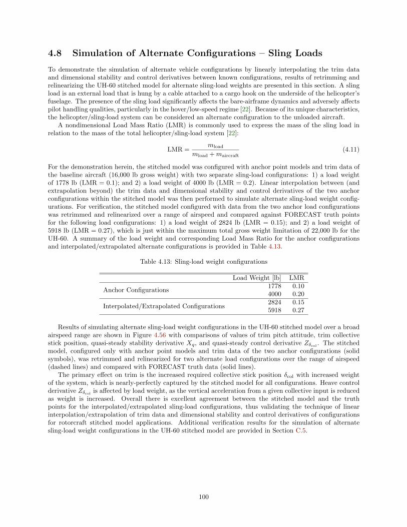
4.8 Simulation of Alternate Configurations – Sling Loads

To demonstrate the simulation of alternate vehicle configurations by linearly interpolating the trim dataand dimensional stability and control derivatives between known configurations, results of retrimming andrelinearizing the UH-60 stitched model for alternate sling-load weights are presented in this section. A slingload is an external load that is hung by a cable attached to a cargo hook on the underside of the helicopter’sfuselage. The presence of the sling load significantly affects the bare-airframe dynamics and adversely affectspilot handling qualities, particularly in the hover/low-speed regime [22]. Because of its unique characteristics,the helicopter/sling-load system can be considered an alternate configuration to the unloaded aircraft.

A nondimensional Load Mass Ratio (LMR) is commonly used to express the mass of the sling load inrelation to the mass of the total helicopter/sling-load system [22]:

LMR =mload

mload +maircraft(4.11)

For the demonstration herein, the stitched model was configured with anchor point models and trim data ofthe baseline aircraft (16,000 lb gross weight) with two separate sling-load configurations: 1) a load weightof 1778 lb (LMR = 0.1); and 2) a load weight of 4000 lb (LMR = 0.2). Linear interpolation between (andextrapolation beyond) the trim data and dimensional stability and control derivatives of the two anchorconfigurations within the stitched model was then performed to simulate alternate sling-load weight config-urations. For verification, the stitched model configured with data from the two anchor load configurationswas retrimmed and relinearized over a range of airspeed and compared against FORECAST truth pointsfor the following load configurations: 1) a load weight of 2824 lb (LMR = 0.15); and 2) a load weight of5918 lb (LMR = 0.27), which is just within the maximum total gross weight limitation of 22,000 lb for theUH-60. A summary of the load weight and corresponding Load Mass Ratio for the anchor configurationsand interpolated/extrapolated alternate configurations is provided in Table 4.13.

Table 4.13: Sling-load weight configurations

Load Weight [lb] LMR

Anchor Configurations1778 0.104000 0.20

Interpolated/Extrapolated Configurations2824 0.155918 0.27

Results of simulating alternate sling-load weight configurations in the UH-60 stitched model over a broadairspeed range are shown in Figure 4.56 with comparisons of values of trim pitch attitude, trim collectivestick position, quasi-steady stability derivative Xq, and quasi-steady control derivative Zδcol . The stitchedmodel, configured only with anchor point models and trim data of the two anchor configurations (solidsymbols), was retrimmed and relinearized for two alternate load configurations over the range of airspeed(dashed lines) and compared with FORECAST truth data (solid lines).

The primary effect on trim is the increased required collective stick position δcol with increased weightof the system, which is nearly-perfectly captured by the stitched model for all configurations. Heave controlderivative Zδcol is affected by load weight, as the vertical acceleration from a given collective input is reducedas weight is increased. Overall there is excellent agreement between the stitched model and the truthpoints for the interpolated/extrapolated sling-load configurations, thus validating the technique of linearinterpolation/extrapolation of trim data and dimensional stability and control derivatives of configurationsfor rotorcraft stitched model applications. Additional verification results for the simulation of alternatesling-load weight configurations in the UH-60 stitched model are provided in Section C.5.

100

-4

-2

0

2

4

6

8

θ [d

eg]

0 40 80 1204

4.5

5

5.5

6

6.5

7

δ col [i

n]

Airspeed [kn]

2

4

6

8

10

12

14

Xq

0 40 80 120-8

-7.5

-7

-6.5

-6

-5.5

-5

-4.5

Zδ co

l

Airspeed [kn]

Stitched Model

0.1

0.15

0.2

0.27

Truth Load Mass RatioAnchor Pt.

Figure 4.56: Alternate configuration verification, sling-load weight.

4.9 Flight-Test Implications for Rotorcraft

A key application of the model stitching architecture is the development of full flight-envelope stitchedsimulation models from flight-identified point models using system identification methods and associatedflight-test trim data. This section covers the overall considerations for planning and conducting a flight testinvolving rotorcraft for the development of stitched simulation models. The techniques and requirementspresented in this section follow closely to those for fixed-wing applications presented earlier in Section 3.9,with the pertinent material referenced throughout. Analyses of the FORECAST UH-60 simulation modeldata trends discussed herein and lessons learned are applied to provide specific guidance for rotorcraft onthe spacing and quantity of trim data, point models, and static stability data to be obtained in flight testing.A summary of the overall flight-test recommendations for rotorcraft is provided in Table 4.14.

4.9.1 Flight-Test Data Collection

Trim Data

The collection of trim test data is accomplished by trimming the rotorcraft at the desired flight conditionand recording data for a duration of approximately 3–5 seconds. Post-flight processing of the data is doneto determine the average trim values of the controls, aircraft attitude, and any additional desired states forthe particular flight-test point. As with fixed-wing aircraft, it is important to know the helicopter loading

101

configuration at each test point (e.g., from measurements of the fuel load at each test point for use witha fuel-burn data sheet post-flight) as the trim points are then collectively baselined to a nominal loadingduring data processing, as discussed in Section 4.9.2.

It is necessary to collect fine-increment trim points around hover to accurately capture the migration ofcontrols and helicopter attitude for the simulation of low-speed forward, rearward, sideward, and quarteringflight, as well as the simulation of hovering flight in the presence of winds. The spacing and correspondinggradients between the trim data affect the accuracy of the implicit speed derivatives of the hover identificationpoint model, as presented in Section 4.3, so a fine spacing of 3–5 kn is recommended for pure forward (i.e.,0 deg), rearward (i.e., 180 deg), and sideward (i.e., 90 and 270 deg) flight up to approximately 20 kn.Additionally, quartering flight points should be collected at 45-deg radial increments (i.e., 45, 135, 225, and315 deg) at a fine airspeed increment of 5 kn total airspeed.

In forward flight, it is important to capture critical inflections in the trim curves (e.g., bottom of thepower curve) for accurate simulation over the forward-flight airspeed envelope. Collecting trim data at asomewhat-fine 10-kn speed increment up to a forward airspeed of 80 knots is recommended to ensure thecapture of key trim trends (see Section 4.4). Collecting trim data at a coarser 20-kn speed increment athigher airspeeds (i.e., > 80 kn) is satisfactory, as was done for the UH-60 stitched model presented herein.

Identification Point Models

The process of identifying point models in rotorcraft is identical to that for fixed-wing aircraft (see Sec-tion 3.9.1), and involves performing frequency sweeps in each primary axis and processing the flight-testdata to extract state-space models at each flight-test condition. The analyses of the FORECAST UH-60model stability and control derivative trends over ranges of airspeed (Section 4.6) show that 4 identifiedpoint models are sufficient to accurately represent the dynamic response of the rotorcraft over the entireairspeed range for a particular altitude. Identification point models are typically valid over ±20 kn fromthe ID airspeed, so a 40-kn spacing is recommended. Identification point models were therefore includedat hover, 40, 80, and 120 knots for the UH-60 stitched model presented herein. As with the collection oftrim data, it is important to note the loading configuration at the start of each frequency sweep run, as thisinformation is used during the baselining process.

Static Stability Data

When performing system identification it is common for speed derivatives to be insensitive due to lackof frequency response data at low frequencies. Therefore it is recommended that longitudinal and lat-eral/directional static stability data be collected around each point for which a model is identified, whichcan be used to explicitly calculate speed derivatives Mu and Lv, and static-stability derivative Nv [1].

For hover/low-speed flight the “collective-fixed” [23] method for obtaining longitudinal and lateral staticstability data is suggested. Here, the collective is held constant at “power for level flight” (i.e., zero climbrate) while the cyclic stick is used to vary forward/rearward airspeed for longitudinal data, and sidewardairspeed for lateral data. Collecting the static stability data over a range of approximately −15 to +15 knotsaround the hover point model flight condition, at an increment of approximately 5 knots, is suggested toaccurately capture the Mu, Lv, and Nv derivatives.

In forward flight, the above “collective-fixed” method is equally applicable for obtaining longitudinalstatic stability data. It is recommended that longitudinal static stability data be collected around eachforward-flight flight condition for which a point model is identified, using the above guidance on airspeedchange and spacing. Lateral/directional static stability data should be collected in forward flight using the“steady heading sideslip” [23] technique.

While the primary purpose of the static stability data is for accurate identification of the Mu, Lv, andNv derivatives in the point models, these data do provide an additional, finely-spaced source of trim dataaround the identification flight conditions. However, these collected data must be processed (i.e., retrimmed)to a level flight path angle using the model stitching architecture to be combined with the collected trimdata, as discussed in Section 4.9.2.

102

Verification Doublets

Performing piloted doublets at each point for which a model is identified is useful for time-domain verificationof the identified point models and the final stitched model at the anchor point flight conditions. Two doublets,one each for a positive and negative input, in each of the primary axes at each identified point model flightcondition are required for verification.

4.9.2 Data Processing

Baselining

Typically during flight testing there will be a natural variance in helicopter weight between test points dueto fuel burn-off, which will also affect the inertia values and CG location. As a result, the precise loadingconfiguration will likely vary among the anchor points. To remove the effects of loading configuration on trimand dynamics, a method was introduced in Section 3.9.2 in which the anchor trim data and identified pointmodels are baselined to a nominal, or baseline, loading configuration using the model stitching simulationarchitecture. In this process, the integrated extrapolation methods (Section 2.5) are employed to accuratelyretrim the anchor trim points and relinearize the anchor point models to a common loading configuration.These baselined anchor points are then used to construct the final stitched model.

As with fixed-wing applications, static stability data collected using the collective-fixed method must alsobe baselined (i.e., retrimmed) to a level flight path angle using the model stitching architecture to employthe data as additional trim points. This is accomplished by ensuring the climb or descent rate is capturedin the collected flight-test data, then simply retrimming each data point to level flight.

Interpolation

Upon completion of the baselining processing step, the full collection of data is then further processed fordirect use in the model stitching architecture. These processing steps include the fitting of splines to thedata and interpolating the data to a fine grid. Trim data must be formatted as a full rectangular grid,which is a grid constructed from defined axis values for each interpolation dimension, per requirements ofthe model stitching architecture interpolation scheme (see Section 2.9). Typically, the grid will be defined fora set range of x-body airspeed U (and y-body airspeed V in the hover/low-speed regime) and a set range ofaltitude, covering the entire flight envelope. Employing 2-D spline interpolation around hover, for example,as discussed in Section 4.5, allows the collected data to be interpolated to the defined grid while retainingcritical inflections in the data.

4.9.3 Rotorcraft Configurations

The extrapolation methods integrated into the model stitching architecture were shown to very accuratelysimulate loading configurations with off-nominal values of weight, CG, and inertia (see Section 4.6). There-fore, collecting trim data and identifying point models is necessary using only the nominal (baseline) rotor-craft configuration. If the simulation of additional off-nominal configurations is desired, such as the aircraftconfigured with an external sling load, that configuration would need to be identified or sufficiently modeledby the user for accurate simulation results.

4.9.4 Altitude

Collecting trim data and identifying models at two altitudes is essential for capturing the behavior of ro-torcraft trim and key stability and control derivatives over a reasonable operational altitude envelope. Forthe UH-60 stitched model example presented herein, the technique of linear interpolation/extrapolation ofthe anchor points at altitudes of sea level and 6000 ft yielded very good agreement over a broad altituderange of sea level through 10,000 ft (see Section 4.6.4). Based on these results, it is suggested that trimis collected and models are identified at sea level and 6000 feet. A 6000-ft spacing was also chosen whenidentifying models of the Bell 206 at 1000 ft and 7000 ft for the development of a stitched simulation model,as presented in Ref. [5], which yielded good results.

103

4.9.5 Summary of Recommendations

The overall flight-test recommendations for the development of a rotorcraft stitched simulation model aresummarized in Table 4.14. These recommendations are based on the analyses of the FORECAST UH-60stitched simulation model presented herein, and are appropriate for military and civilian conventional heli-copter applications. The table provides recommended airspeed increments, quantity of points, and exampleprofile at which to identify point models and collect trim data. Trim data recommendations are further or-ganized into forward/rearward points for hover/low-speed through forward flight, and sideward/quarteringpoints for hover/low-speed. Recommended altitudes at which to perform the data collection are provided.

Table 4.14: Summary of flight-test recommendations for development of rotorcraft stitched models

InterpolationDimension

Parameter ID Point Models Trim Data

Airspeed

Forward/Rearward Sideward/Quartering# of airspeeds 3–5 15–20 15–25Increment [kn] 40–60 5–20a,b 3–5c

Example profile [hover 40 80 120] [−20 −15 −10 −5hover 5 10 15 20 3040 50 60 70 80 100 120140 160]

[5 10 15 20] kn@ [45 90 135 225 270315] deg

Altitude# of altitudes 2 2Increment [ft] 5000–7000 5000–7000Example profile [sea level 6000] [sea level 6000]

a Fine 5-kn increment around hover (≤ 20 kn), 10-kn increment at low/mid speed (≤ 80 kn), and coarser 20-kn incrementout to high speed (> 80 kn)

b Can include baselined longitudinal static stability data as fine-increment trim data around ID pointsc Can include baselined lateral static stability data as fine-increment sideward trim data around the hover ID point


Application of the model stitching architecture for a rotorcraft was demonstrated in this chapter usingFORECAST high-order linear models of the UH-60 Black Hawk helicopter. In addition to demonstratingthe use of high-order models in the model stitching architecture, this example application also demonstratedthe storing and subsequent look-up of trim data in multiple dimensions. Stitching in x-body axis airspeedU and y-body axis airspeed V allowed for accurate simulation in the hover/low-speed regime. Scenarioswere investigated to determine recommended spacing and strategies for the collection of trim data in thehover/low-speed and forward-flight regimes.

Verification results of the off-nominal extrapolation methods were presented comparing outputs of thestitched model to values from point models for off-nominal configurations and conditions. Two check caseswere provided to verify overall simulation fidelity at two discrete flight conditions and configurations. Find-ings and implications were considered to provide guidance on future flight testing for the development ofstitched models involving rotorcraft.

104

5 Conclusions

Model stitching is a technique that allows continuous, full flight-envelope flight dynamics simulation of fixed-wing aircraft and rotorcraft using only a small number of discrete-point linear models and trim data. Amodel stitching simulation architecture has been developed, which allows flight-identified models to be useddirectly, and incorporates additional features and extrapolation methods for the simulation of off-nominalloading configurations and alternate altitudes. The model stitching simulation architecture is applicableto any flight vehicle configuration for which point-wise linear models and trim data can be obtained, andis demonstrated herein for a fixed-wing aircraft model representative of the Cessna Citation CJ1 and arotorcraft model representative of the UH-60 Black Hawk.

The following general conclusions were determined from the current effort:

1. The model stitching simulation architecture provides a quasi-nonlinear, time varying model that isaccurate for flight dynamics and control applications over the operational envelope, with good accuracymaintained in the frequency- and time-domain.

2. For both the fixed-wing CJ1 and the UH-60 rotorcraft application, configuring the stitched simulationmodels with 8 discrete-point linear models (4 point models each at two altitudes) plus additional trimdata, and employing the appropriate altitude extrapolation technique for each case, was found to allowaccurate simulation over the full airspeed and altitude range.

3. Accurate simulation of off-nominal aircraft configurations (i.e., values of gross weight, inertia, and CGlocation that differ from those of the identified/baseline configuration) is accomplished by real-timeextrapolation methods within the model stitching architecture. The off-nominal extrapolation methodsnecessitate only the baseline aircraft loading configuration to be flight tested, which significantly reducesrequired flight-test points and associated flight costs.

Fixed-Wing Aircraft

The following conclusions were determined from the analyses of the Cessna Citation CJ1 stitched model:

i. The model stitching technique of combining linear point models and trim data for discrete flightconditions allows for accurate, full flight-envelope simulation of a business jet. Eight discrete pointmodels (4 at 10,000 ft and 4 at 30,000 ft) over the airspeed range and at a nominal weight/CG areneeded to cover the flight envelope and accurately predict off-nominal trends. More finely-spaced trimdata are also needed to correctly capture trends and key inflections.

ii. Point models and trim data at two altitudes provides for an accurate simulation of altitude effects usingair density-ratio scaling. Extrapolating models to off-nominal altitudes using air density-ratio scalingwas found to be highly accurate over a range of ±10,000 ft for the CJ1 stitched model application.Extrapolation on two sets of point models and trim data were performed; the 10,000-ft data wereextrapolated to sea level and 20,000 ft, and the 30,000-ft data were extrapolated to 40,000 ft, coveringthe entire altitude envelope in 10,000-ft increments. Air density-ratio scaling produced more accurateresults than linearly interpolating between the two altitudes.

iii. Analyses of the nondimensional stability and control derivatives from the AAA CJ1 model have in-dicated that some nondimensional derivatives are significantly affected by Mach and angle-of-attackeffects, and are not necessarily constant over the flight envelope. As such, the flight-test recommenda-tions for the identification of 4 point models each at two altitudes is appropriate using either dimensionalderivatives or nondimensional derivatives.

iv. Analyses of variations in trim and derivative values from the AAA CJ1 model as a function of flap de-flection indicate significant changes in trim angle of attack, elevator deflection, and thrust for deployedflaps at a given airspeed. Although some stability and control derivatives are affected, the largest

105

and most significant variations with flap deflection are seen in trim angle of attack and longitudinalcontrols. Herein, the flap deflection implementation was confined to changes in trim only; the stabilityand control derivatives remain at the nominal (i.e., flaps-up) configuration. This approach ensures thattrim with flap deflection is correct, which is important for piloted simulation, and allows for efficientflight testing while satisfactorily preserving the dynamic response.

Rotorcraft

The following conclusions were determined from the analyses of the UH-60 Black Hawk stitched model:

i. Full flight-envelope simulation using the model stitching simulation architecture was demonstrated fora rotorcraft application, requiring only 8 discrete point models (4 at sea level and 4 at 6000 ft) at anominal weight/CG. More finely-spaced trim data are also needed to correctly capture trends and keyinflections.

ii. Storing and subsequent look-up of trim data in multiple simultaneous dimensions, i.e., stitching in x-body airspeed U and y-body airspeed V , has been demonstrated to yield good accuracy of the UH-60stitched simulation model in the hover/low-speed regime. Low-speed forward, rearward, and sidewardtrim data at a fine 5-kn increment, as well as quartering flight trim at 45-deg radial spacing, was foundto accurately preserve the implicit u- and v-speed derivative values, and thus the dynamic response,around hover. Additionally, hovering flight in the presence of steady winds was accurately simulatedusing the above trim data collection strategy.

iii. High-order linear models can be effectively utilized in the model stitching architecture. Dynamicresponse check cases provided verification of the higher-order rotor dynamics for two flight conditionsat off-nominal loading configurations.

iv. Linear interpolation, as opposed to air density-ratio scaling, between data at anchor altitudes is recom-mended for simulating off-nominal altitudes for rotorcraft, as certain derivatives do not scale directlywith altitude. Herein, linear interpolation was performed on trim data and derivatives between thesea-level and 6000-ft anchor data, and the data were also linearly extrapolated to 10,000 ft, whichyielded good results.

106

Appendix A Stability and Control Derivatives for

Fixed-Wing Aircraft

Contents

A.1 Stability Axes Coordinate System . . . . . . . . . . . . . . . . . . . . . . . . . . . . . . . . . . 107A.1.1 Inertias . . . . . . . . . . . . . . . . . . . . . . . . . . . . . . . . . . . . . . . . . . . . 107A.1.2 Unprimed Dimensional Derivatives . . . . . . . . . . . . . . . . . . . . . . . . . . . . . 107A.1.3 Primed Dimensional Derivatives . . . . . . . . . . . . . . . . . . . . . . . . . . . . . . 109

A.2 Body Axes Coordinate System . . . . . . . . . . . . . . . . . . . . . . . . . . . . . . . . . . . 109A.2.1 Derivative Transformations . . . . . . . . . . . . . . . . . . . . . . . . . . . . . . . . . 109A.2.2 Thrust Control Derivatives . . . . . . . . . . . . . . . . . . . . . . . . . . . . . . . . . 110

This Appendix provides stability and control derivative definitions and conversions used in the devel-opment of the bare-airframe models for the Cessna Citation CJ1 stitched model presented in Chapter 3.The bare-airframe linear point models were first formulated in stability axes then transformed into bodyaxes for use in the model stitching simulation architecture. Section A.1 provides equations for the calcula-tion of stability-axes inertias, dimensional derivatives from nondimensional derivatives, and primed deriva-tives. Section A.2 provides transformation equations to obtain body-axes dimensional derivatives given thestability-axes dimensional derivatives. Equations for the thrust control derivatives are given in Section A.2.2.

A.1 Stability Axes Coordinate System

A.1.1 Inertias

Given the values of the aircraft moments of inertia (Ixx, Iyy, and Izz) and cross-product of inertia Ixz inbody axes, the values of the stability-axes inertias are found following Ref. [13]:

Ixxs = Ixx cos2 α0 + Izz sin2 α0 − Ixz sin 2α0 (A.1)

Iyys = Iyy (A.2)

Izzs = Ixx sin2 α0 + Izz cos2 α0 + Ixz sin 2α0 (A.3)

Ixzs = 12 (Ixx − Izz) sin 2α0 + Ixz cos 2α0 (A.4)

where α0 is the trim angle of attack. The stability-axes inertias are used in the calculation of the dimensionalstability-axes derivatives, as presented in Sections A.1.2 and A.1.3.

A.1.2 Unprimed Dimensional Derivatives

Dimensional stability and control derivatives in stability axes are found from the nondimensional derivativesand aircraft properties [13]:

Xu =−qSmVtot0

(2CD + CDu) (A.5)

XTu =qS

mVtot0

(2CT + CTu) (A.6)

Xα =qS

m(CL − CDα) (A.7)

Xw =Xα

Vtot0

(A.8)

107

Xδe =−qSm

CDδe (A.9)

Zu =−qSmVtot0

(2CL + CLu) (A.10)

Zα =−qSm

(CD + CLα) (A.11)

Zw =ZαVtot0

(A.12)

Zα =−qSc

2mVtot0

CLα (A.13)

Zw =ZαVtot0

(A.14)

Zq =−qSc

2mVtot0

CLq (A.15)

Zδe =−qSm

CLδe (A.16)

Mu =qSc

IyyVtot0

(2Cm + Cmu) (A.17)

MTu =qSc

IyyVtot0

(2CmT + CmTu

)(A.18)

Mα =qSc

IyyCmα (A.19)

Mw =Mα

Vtot0

(A.20)

Mα =qSc

Iyy

c

2Vtot0

Cmα (A.21)

Mw =Mα

Vtot0

(A.22)

Mq =qSc

Iyy

c

2Vtot0

Cmq (A.23)

Mδe =qSc

IyyCmδe (A.24)

Yβ =qS

mCYβ (A.25)

Yv =YβVtot0

(A.26)

Yp =qSb

2mVtot0

CYp (A.27)

Yr =qSb

2mVtot0

CYr (A.28)

Yδr =qS

mCYδr (A.29)

Yδa =qS

mCYδa (A.30)

Lβ =qSb

Ixxs

Clβ (A.31)

Lv =LβVtot0

(A.32)

108

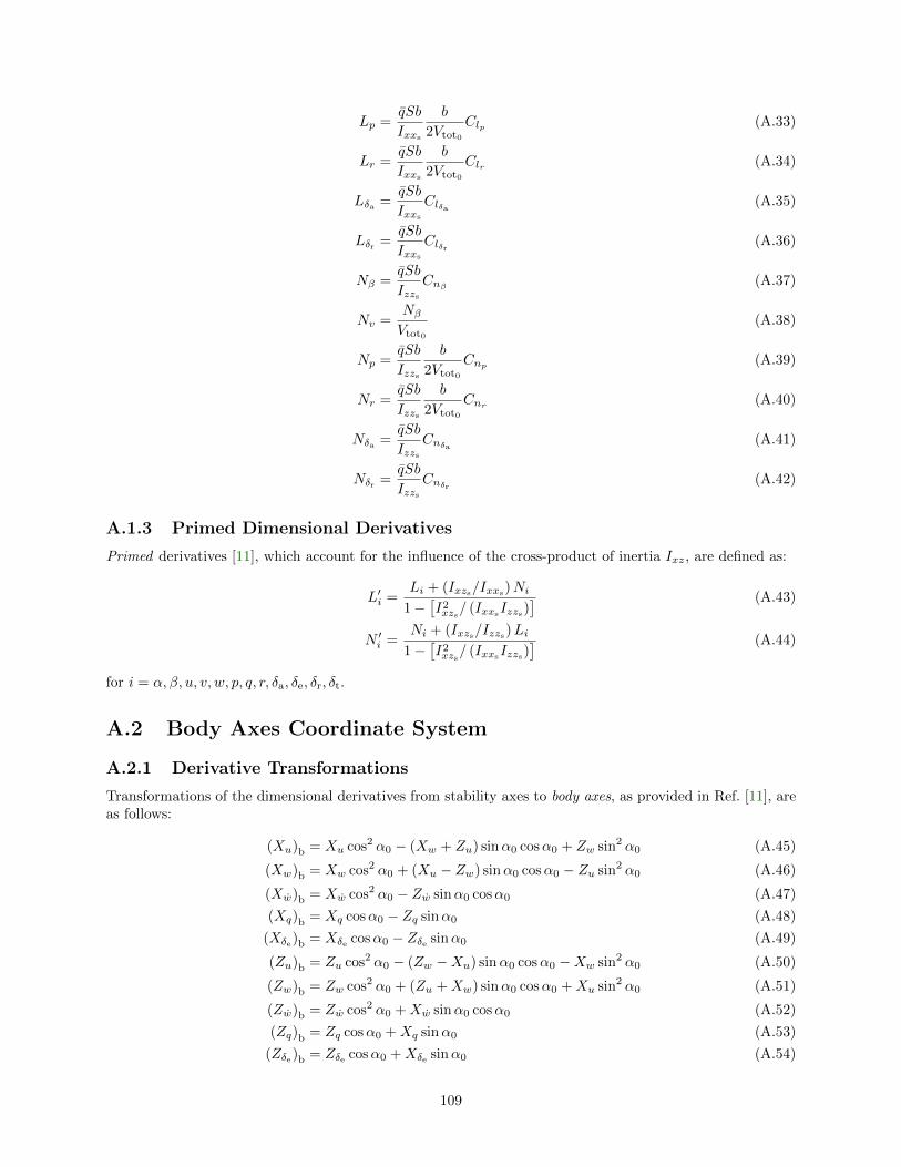
Lp =qSb

Ixxs

b

2Vtot0

Clp (A.33)

Lr =qSb

Ixxs

b

2Vtot0

Clr (A.34)

Lδa =qSb

Ixxs

Clδa (A.35)

Lδr =qSb

Ixxs

Clδr (A.36)

Nβ =qSb

IzzsCnβ (A.37)

Nv =NβVtot0

(A.38)

Np =qSb

Izzs

b

2Vtot0

Cnp (A.39)

Nr =qSb

Izzs

b

2Vtot0

Cnr (A.40)

Nδa =qSb

IzzsCnδa (A.41)

Nδr =qSb

IzzsCnδr (A.42)

A.1.3 Primed Dimensional Derivatives

Primed derivatives [11], which account for the influence of the cross-product of inertia Ixz, are defined as:

L′i =Li + (Ixzs/Ixxs

)Ni

1−[I2xzs/ (Ixxs

Izzs)] (A.43)

N ′i =Ni + (Ixzs/Izzs)Li

1−[I2xzs/ (IxxsIzzs)

] (A.44)

for i = α, β, u, v, w, p, q, r, δa, δe, δr, δt.

A.2 Body Axes Coordinate System

A.2.1 Derivative Transformations

Transformations of the dimensional derivatives from stability axes to body axes, as provided in Ref. [11], areas follows:

(Xu)b = Xu cos2 α0 − (Xw + Zu) sinα0 cosα0 + Zw sin2 α0 (A.45)

(Xw)b = Xw cos2 α0 + (Xu − Zw) sinα0 cosα0 − Zu sin2 α0 (A.46)

(Xw)b = Xw cos2 α0 − Zw sinα0 cosα0 (A.47)

(Xq)b = Xq cosα0 − Zq sinα0 (A.48)

(Xδe)b = Xδe cosα0 − Zδe sinα0 (A.49)

(Zu)b = Zu cos2 α0 − (Zw −Xu) sinα0 cosα0 −Xw sin2 α0 (A.50)

(Zw)b = Zw cos2 α0 + (Zu +Xw) sinα0 cosα0 +Xu sin2 α0 (A.51)

(Zw)b = Zw cos2 α0 +Xw sinα0 cosα0 (A.52)

(Zq)b = Zq cosα0 +Xq sinα0 (A.53)

(Zδe)b = Zδe cosα0 +Xδe sinα0 (A.54)

109

(Mu)b = Mu cosα0 −Mw sinα0 (A.55)

(Mw)b = Mw cosα0 +Mu sinα0 (A.56)

(Mw)b = Mw cosα0 (A.57)

(Mq)b = Mq (A.58)

(Mδe)b = Mδe (A.59)

(Yv)b = Yv (A.60)

(Yp)b = Yp cosα0 − Yr sinα0 (A.61)

(Yr)b = Yr cosα0 + Yp sinα0 (A.62)

(Yδa)b = Yδa (A.63)

(Yδr)b = Yδr (A.64)

(L′v)b = L′v cosα0 −N ′v sinα0 (A.65)(L′p)

b= L′p cos2 α0 −

(L′r +N ′p

)sinα0 cosα0 +N ′r sin2 α0 (A.66)

(L′r)b = L′r cos2 α0 −(N ′r − L′p

)sinα0 cosα0 −N ′p sin2 α0 (A.67)(

L′δa)

b= L′δa cosα0 −N ′δa sinα0 (A.68)(

L′δr)

b= L′δr cosα0 −N ′δr sinα0 (A.69)

(N ′v)b = N ′v cosα0 + L′v sinα0 (A.70)(N ′p)

b= N ′p cos2 α0 −

(N ′r − L′p

)sinα0 cosα0 − L′r sin2 α0 (A.71)

(N ′r)b = N ′r cos2 α0 +(L′r +N ′p

)sinα0 cosα0 + L′p sin2 α0 (A.72)(

N ′δa)

b= N ′δa cosα0 + L′δa sinα0 (A.73)(

N ′δr)

b= N ′δr cosα0 + L′δr sinα0 (A.74)

Note that the above body-axes notation ( )b is dropped elsewhere herein.

A.2.2 Thrust Control Derivatives

The dimensional thrust control derivatives are formulated based on the geometric placement and incidenceof the engines, and the assumption that the produced thrust is concentrated at the center of the enginenacelle. The thrust derivatives are naturally defined in body axes as follows:

Xδt =1

mcosαt (A.75)

Zδt = − 1

msinαt (A.76)

Mδt =1

Iyy(zt cosαt + xt sinαt) (A.77)

where αt is the thrust inclination angle, and xt and zt are the x- and z-axis offsets, respectively, between thethrust center and the aircraft CG. The thrust control input δt has units of pounds thrust, and an assumedrange from 0 to maximum thrust.

110

Appendix B Verification Figures: CJ1 Stitched Model

Contents

B.1 Weight . . . . . . . . . . . . . . . . . . . . . . . . . . . . . . . . . . . . . . . . . . . . . . . . . 112B.2 Inertia . . . . . . . . . . . . . . . . . . . . . . . . . . . . . . . . . . . . . . . . . . . . . . . . . 116

B.2.1 Roll Inertia . . . . . . . . . . . . . . . . . . . . . . . . . . . . . . . . . . . . . . . . . . 116B.2.2 Pitch Inertia . . . . . . . . . . . . . . . . . . . . . . . . . . . . . . . . . . . . . . . . . 120B.2.3 Yaw Inertia . . . . . . . . . . . . . . . . . . . . . . . . . . . . . . . . . . . . . . . . . . 123

B.3 Center of Gravity . . . . . . . . . . . . . . . . . . . . . . . . . . . . . . . . . . . . . . . . . . . 126B.3.1 Station CG . . . . . . . . . . . . . . . . . . . . . . . . . . . . . . . . . . . . . . . . . . 126B.3.2 Waterline CG . . . . . . . . . . . . . . . . . . . . . . . . . . . . . . . . . . . . . . . . . 130

B.4 Altitude . . . . . . . . . . . . . . . . . . . . . . . . . . . . . . . . . . . . . . . . . . . . . . . . 134B.4.1 Single-Altitude Data – 10,000 ft . . . . . . . . . . . . . . . . . . . . . . . . . . . . . . 134B.4.2 Single-Altitude Data – 30,000 ft . . . . . . . . . . . . . . . . . . . . . . . . . . . . . . 138B.4.3 Data from Two Altitudes – 10,000 ft and 30,000 ft . . . . . . . . . . . . . . . . . . . . 142

B.5 Flap Setting . . . . . . . . . . . . . . . . . . . . . . . . . . . . . . . . . . . . . . . . . . . . . . 146

This appendix provides additional off-nominal verification results for the Cessna Citation CJ1 businessjet stitched model, as presented in Section 3.6. Stability and control derivative and trim comparisons areprovided for a range of airspeed for off-nominal values of weight (Section B.1), inertia (Section B.2), centerof gravity location (Section B.3), altitude (Section B.4), and flap setting (Section B.5). In all figures, thestitched model, configured only with the anchor point models and trim data indicated (solid symbols), wasretrimmed and relinearized for various simulation values of each property over a range of airspeed (dashedlines) and compared with values from the AAA truth data (solid lines).

111

B.1 Weight

Figures B.1–B.3 show the complete trim and stability and control derivative comparison results for the CJ1off-nominal weight verification presented in Section 3.6.1.

0

5

10

α [d

eg]

-15

-10

-5

0

5

δ e [deg

]

100 150 200 250 300 350 400

500

1000

1500

2000

δ t [lb]

Airspeed [kn]

Stitched Model

6000

7250

8500

9750


Figure B.1: Verification of off-nominal weight extrapolation, CJ1 stitched model, trim.

112

-0.04

-0.03

-0.02

-0.01

0

Xu

-0.25

-0.2

-0.15

-0.1

-0.05

Zu

-5

0

5

10x 10

-3

Mu

-0.8

-0.6

-0.4

-0.2

0

Yv

-0.06

-0.04

-0.02

0

L v

100 150 200 250 300 350 4000.005

0.01

0.015

0.02

Nv

Airspeed [kn]

-0.1

0

0.1

0.2

0.3

Xw

-6

-4

-2

0

Zw

100 150 200 250 300 350 400-0.2

-0.15

-0.1

-0.05

0

Mw

Airspeed [kn]

Stitched Model

6000

7250

8500

9750


Figure B.2: Verification of off-nominal weight extrapolation, CJ1 stitched model, stability derivatives.

113

-1

0

1

2X

q

-40

-30

-20

-10

0

Zq

-8

-6

-4

-2

0

Mq

-3

-2

-1

0

Yp

-8

-6

-4

-2

L p

100 150 200 250 300 350 400-0.7

-0.6

-0.5

-0.4

-0.3

Np

Airspeed [kn]

0

2

4

6

Yr

0.4

0.5

0.6

0.7

0.8

L r

100 150 200 250 300 350 400-0.8

-0.6

-0.4

-0.2

0

Nr

Airspeed [kn]

Stitched Model

6000

7250

8500

9750


Figure B.2: Verification of off-nominal weight extrapolation, CJ1 stitched model, stability derivatives (cont.)

114

-10

-5

0

5

Xδ e

-300

-200

-100

0

Zδ e

-60

-40

-20

0

Mδ e

0

20

40

60

L δ a

100 150 200 250 300 350 4000

1

2

3

Nδ a

Airspeed [kn]

3

4

5

6x 10

-3

Xδ t

-3

-2.5

-2

-1.5x 10

-4

Zδ t

-1.472

-1.47

-1.468

-1.466x 10

-4

Mδ t

0

50

100

Yδ r

0

2

4

6

L δ r

100 150 200 250 300 350 400-15

-10

-5

0

Nδ r

Airspeed [kn]

Stitched Model

6000

7250

8500

9750


Figure B.3: Verification of off-nominal weight extrapolation, CJ1 stitched model, control derivatives.

115

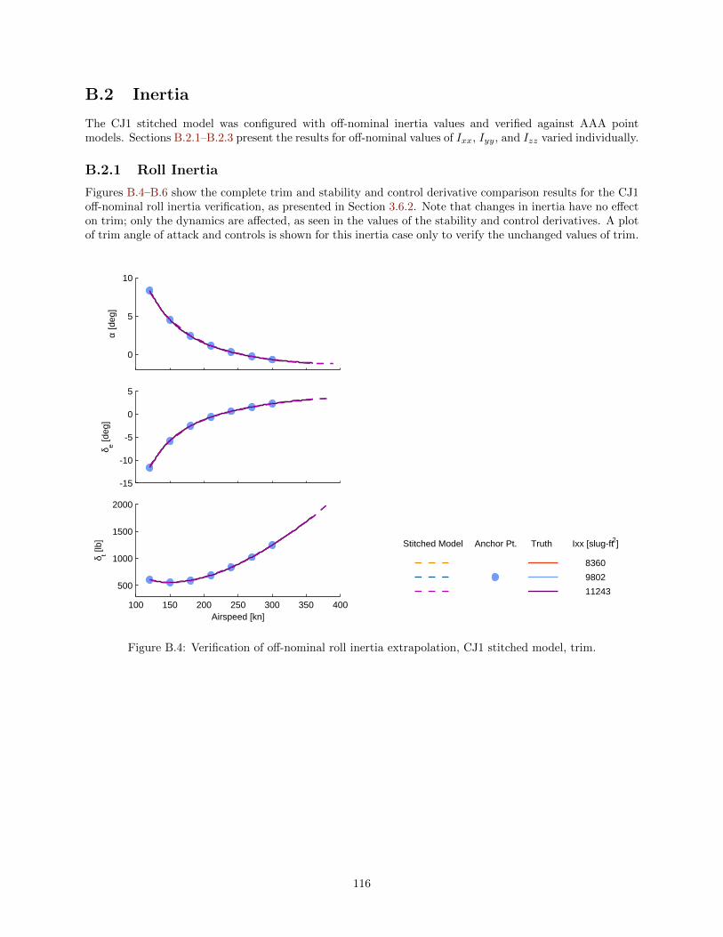
B.2 Inertia

The CJ1 stitched model was configured with off-nominal inertia values and verified against AAA pointmodels. Sections B.2.1–B.2.3 present the results for off-nominal values of Ixx, Iyy, and Izz varied individually.

B.2.1 Roll Inertia

Figures B.4–B.6 show the complete trim and stability and control derivative comparison results for the CJ1off-nominal roll inertia verification, as presented in Section 3.6.2. Note that changes in inertia have no effecton trim; only the dynamics are affected, as seen in the values of the stability and control derivatives. A plotof trim angle of attack and controls is shown for this inertia case only to verify the unchanged values of trim.

0

5

10

α [d

eg]

-15

-10

-5

0

5

δ e [deg

]

100 150 200 250 300 350 400

500

1000

1500

2000

δ t [lb]

Airspeed [kn]

Stitched Model

8360

9802

11243


Figure B.4: Verification of off-nominal roll inertia extrapolation, CJ1 stitched model, trim.

116

-0.03

-0.02

-0.01

0

Xu

-0.25

-0.2

-0.15

-0.1

Zu

-5

0

5

10x 10

-3

Mu

-0.4

-0.3

-0.2

-0.1

0

Yv

-0.06

-0.04

-0.02

0

L v

100 150 200 250 300 350 4000.005

0.01

0.015

0.02

Nv

Airspeed [kn]

-0.1

0

0.1

0.2

0.3

Xw

-4

-3

-2

-1

0

Zw

100 150 200 250 300 350 400-0.2

-0.15

-0.1

-0.05

0

Mw

Airspeed [kn]

Stitched Model

8360

9802

11243


Figure B.5: Verification of off-nominal roll inertia extrapolation, CJ1 stitched model, stability derivatives.

117

-0.5

0

0.5

1X

q

-25

-20

-15

-10

-5

Zq

-8

-6

-4

-2

0

Mq

-2

-1.5

-1

-0.5

0

Yp

-10

-5

0

L p

100 150 200 250 300 350 400-0.7

-0.6

-0.5

-0.4

-0.3

Np

Airspeed [kn]

1

2

3

4

Yr

0.4

0.6

0.8

1

L r

100 150 200 250 300 350 400-0.8

-0.6

-0.4

-0.2

0

Nr

Airspeed [kn]

Stitched Model

8360

9802

11243


Figure B.5: Verification of off-nominal roll inertia extrapolation, CJ1 stitched model, stability derivatives(cont.)

118

-10

-5

0

5

Xδ e

-200

-150

-100

-50

0

Zδ e

-60

-40

-20

0

Mδ e

0

20

40

60

80

L δ a

100 150 200 250 300 350 4000

1

2

3

4

Nδ a

Airspeed [kn]

3

3.5

4x 10

-3

Xδ t

-1

-0.5

0x 10

-3

Zδ t

-1

-0.5

0x 10

-3

Mδ t

0

20

40

60

80

Yδ r

0

2

4

6

8

L δ r

100 150 200 250 300 350 400-15

-10

-5

0

Nδ r

Airspeed [kn]

Stitched Model

8360

9802

11243


Figure B.6: Verification of off-nominal roll inertia extrapolation, CJ1 stitched model, control derivatives.

119

B.2.2 Pitch Inertia

Figures B.7 and B.8 show the complete stability and control derivative comparison results for the CJ1off-nominal pitch inertia verification, as presented in Section 3.6.2. As noted and verified in the previoussection, changes in inertia have no effect on trim; thus, the plot showing the unchanged values of trim hasbeen omitted.

-0.03

-0.02

-0.01

0

Xu

-0.25

-0.2

-0.15

-0.1

Zu

-5

0

5

10x 10

-3

Mu

-0.4

-0.3

-0.2

-0.1

0

Yv

100 150 200 250 300 350 400-0.06

-0.04

-0.02

0

L v

Airspeed [kn]

100 150 200 250 300 350 4000.005

0.01

0.015

0.02

Nv

Airspeed [kn]

-0.1

0

0.1

0.2

0.3

Xw

-4

-3

-2

-1

0

Zw

-0.2

-0.15

-0.1

-0.05

0

Mw

Stitched Model

12497

14652

16807

Truth Iyy [slug-ft2]Anchor Pt.

Figure B.7: Verification of off-nominal pitch inertia extrapolation, CJ1 stitched model, stability derivatives.

120

-0.5

0

0.5

1X

q

-25

-20

-15

-10

-5

Zq

-8

-6

-4

-2

0

Mq

-2

-1.5

-1

-0.5

0

Yp

-8

-6

-4

-2

L p

100 150 200 250 300 350 400-0.5

-0.45

-0.4

-0.35

-0.3

Np

Airspeed [kn]

1

2

3

4

Yr

0.55

0.6

0.65

0.7

0.75

L r

100 150 200 250 300 350 400-0.8

-0.6

-0.4

-0.2

0

Nr

Airspeed [kn]

Stitched Model

12497

14652

16807


Figure B.7: Verification of off-nominal pitch inertia extrapolation, CJ1 stitched model, stability derivatives(cont.)

121

-10

-5

0

5

Xδ e

-200

-150

-100

-50

0

Zδ e

-80

-60

-40

-20

0

Mδ e

0

20

40

60

L δ a

100 150 200 250 300 350 4000

1

2

3

Nδ a

Airspeed [kn]

3

3.5

4x 10

-3

Xδ t

-1

-0.5

0x 10

-3

Zδ t

-1.8

-1.6

-1.4

-1.2x 10

-4

Mδ t

0

20

40

60

80

Yδ r

0

2

4

6

L δ r

100 150 200 250 300 350 400-15

-10

-5

0

Nδ r

Airspeed [kn]

Stitched Model

12497

14652

16807


Figure B.8: Verification of off-nominal pitch inertia extrapolation, CJ1 stitched model, control derivatives.

122

B.2.3 Yaw Inertia

Figures B.9 and B.10 show the complete stability and control derivative comparison results for the CJ1off-nominal yaw verification, as presented in Section 3.6.2. As noted and verified previously, changes ininertia have no effect on trim; thus, the plot showing the unchanged values of trim has been omitted fromthis section.

-0.03

-0.02

-0.01

0

Xu

-0.25

-0.2

-0.15

-0.1

Zu

-5

0

5

10x 10

-3

Mu

-0.4

-0.3

-0.2

-0.1

0

Yv

100 150 200 250 300 350 400-0.06

-0.04

-0.02

0

L v

Airspeed [kn]

100 150 200 250 300 350 4000.005

0.01

0.015

0.02

0.025

Nv

Airspeed [kn]

-0.1

0

0.1

0.2

0.3

Xw

-4

-3

-2

-1

0

Zw

-0.2

-0.15

-0.1

-0.05

0

Mw

Stitched Model

20069

23529

26989

Truth Izz [slug-ft2]Anchor Pt.

Figure B.9: Verification of off-nominal yaw inertia extrapolation, CJ1 stitched model, stability derivatives.

123

-0.5

0

0.5

1X

q

-25

-20

-15

-10

-5

Zq

-8

-6

-4

-2

0

Mq

-2

-1.5

-1

-0.5

0

Yp

-8

-6

-4

-2

L p

100 150 200 250 300 350 400-0.7

-0.6

-0.5

-0.4

-0.3

Np

Airspeed [kn]

1

2

3

4

Yr

0.55

0.6

0.65

0.7

0.75

L r

100 150 200 250 300 350 400-0.8

-0.6

-0.4

-0.2

0

Nr

Airspeed [kn]

Stitched Model

20069

23529

26989


Figure B.9: Verification of off-nominal yaw inertia extrapolation, CJ1 stitched model, stability derivatives(cont.)

124

-10

-5

0

5

Xδ e

-200

-150

-100

-50

0

Zδ e

-60

-40

-20

0

Mδ e

0

20

40

60

L δ a

100 150 200 250 300 350 4000

1

2

3

4

Nδ a

Airspeed [kn]

3

3.5

4x 10

-3

Xδ t

-1

-0.5

0x 10

-3

Zδ t

-1

-0.5

0x 10

-3

Mδ t

0

20

40

60

80

Yδ r

0

2

4

6

L δ r

100 150 200 250 300 350 400-20

-15

-10

-5

0

Nδ r

Airspeed [kn]

Stitched Model

20069

23529

26989


Figure B.10: Verification of off-nominal yaw inertia extrapolation, CJ1 stitched model, control derivatives.

125

B.3 Center of Gravity

The CJ1 stitched model was configured with off-nominal CG locations and verified against AAA pointmodels. Section B.3.1 presents the results for off-nominal fuselage-station CG location (x-body axis, positiveaft), and Section B.3.2 presents the results for off-nominal waterline CG location (z-body axis, positive up).

B.3.1 Station CG

Figures B.11–B.13 show the complete trim and stability and control derivative verification results for theCJ1 stitched model configured with fuselage-station CG offsets, as presented in Section 3.6.3.

0

5

10

α [d

eg]

-15

-10

-5

0

5

δ e [deg

]

100 150 200 250 300 350 400

500

1000

1500

2000

δ t [lb]

Airspeed [kn]

Stitched Model

240.1

244.3

248.4


Figure B.11: Verification of off-nominal station CG extrapolation, CJ1 stitched model, trim.

126

-0.03

-0.02

-0.01

0

Xu

-0.25

-0.2

-0.15

-0.1

Zu

-5

0

5

10x 10

-3

Mu

-0.4

-0.3

-0.2

-0.1

0

Yv

-0.06

-0.04

-0.02

0

L v

100 150 200 250 300 350 4000.005

0.01

0.015

0.02

0.025

Nv

Airspeed [kn]

-0.1

0

0.1

0.2

0.3

Xw

-4

-3

-2

-1

0

Zw

100 150 200 250 300 350 400-0.2

-0.15

-0.1

-0.05

0

Mw

Airspeed [kn]

Stitched Model

240.1

244.3

248.4


Figure B.12: Verification of off-nominal station CG extrapolation, CJ1 stitched model, stability derivatives.

127

-0.5

0

0.5

1X

q

-25

-20

-15

-10

-5

Zq

-8

-6

-4

-2

0

Mq

-2

-1.5

-1

-0.5

0

Yp

-8

-6

-4

-2

L p

100 150 200 250 300 350 400-0.5

-0.45

-0.4

-0.35

-0.3

Np

Airspeed [kn]

1

2

3

4

5

Yr

0.55

0.6

0.65

0.7

0.75

L r

100 150 200 250 300 350 400-0.8

-0.6

-0.4

-0.2

0

Nr

Airspeed [kn]

Stitched Model

240.1

244.3

248.4


Figure B.12: Verification of off-nominal station CG extrapolation, CJ1 stitched model, stability derivatives(cont.)

128

-10

-5

0

5

Xδ e

-200

-150

-100

-50

0

Zδ e

-60

-40

-20

0

Mδ e

0

20

40

60

L δ a

100 150 200 250 300 350 4000

1

2

3

Nδ a

Airspeed [kn]

3

3.5

4x 10

-3

Xδ t

-1

-0.5

0x 10

-3

Zδ t

-1

-0.5

0x 10

-3

Mδ t

0

20

40

60

80

Yδ r

0

2

4

6

L δ r

100 150 200 250 300 350 400-15

-10

-5

0

Nδ r

Airspeed [kn]

Stitched Model

240.1

244.3

248.4


Figure B.13: Verification of off-nominal station CG extrapolation, CJ1 stitched model, control derivatives.

129

B.3.2 Waterline CG

Figures B.14–B.16 show the complete trim and stability and control derivative verification results for theCJ1 stitched model configured with waterline CG offsets, as presented in Section 3.6.3.

0

5

10

α [d

eg]

-15

-10

-5

0

5

δ e [deg

]

100 150 200 250 300 350 400

500

1000

1500

2000

δ t [lb]

Airspeed [kn]

Stitched Model

109

113

117

Truth Waterline CG [in]Anchor Pt.

Figure B.14: Verification of off-nominal waterline CG extrapolation, CJ1 stitched model, trim.

130

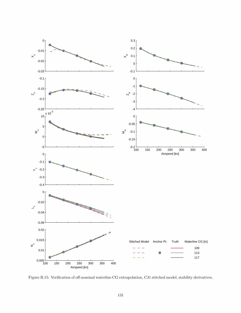
-0.03

-0.02

-0.01

0

Xu

-0.25

-0.2

-0.15

-0.1

Zu

-5

0

5

10x 10

-3

Mu

-0.4

-0.3

-0.2

-0.1

0

Yv

-0.06

-0.04

-0.02

0

L v

100 150 200 250 300 350 4000.005

0.01

0.015

0.02

Nv

Airspeed [kn]

-0.1

0

0.1

0.2

0.3

Xw

-4

-3

-2

-1

0

Zw

100 150 200 250 300 350 400-0.2

-0.15

-0.1

-0.05

0

Mw

Airspeed [kn]

Stitched Model

109

113

117


Figure B.15: Verification of off-nominal waterline CG extrapolation, CJ1 stitched model, stability derivatives.

131

-0.5

0

0.5

1X

q

-25

-20

-15

-10

-5

Zq

-8

-6

-4

-2

0

Mq

-2

-1.5

-1

-0.5

0

Yp

-8

-6

-4

-2

L p

100 150 200 250 300 350 400-0.5

-0.45

-0.4

-0.35

-0.3

Np

Airspeed [kn]

1

2

3

4

Yr

0.5

0.6

0.7

0.8

0.9

L r

100 150 200 250 300 350 400-0.8

-0.6

-0.4

-0.2

0

Nr

Airspeed [kn]

Stitched Model

109

113

117


Figure B.15: Verification of off-nominal waterline CG extrapolation, CJ1 stitched model, stability derivatives(cont.)

132

-10

-5

0

5

Xδ e

-200

-150

-100

-50

0

Zδ e

-60

-40

-20

0

Mδ e

0

20

40

60

L δ a

100 150 200 250 300 350 4000

1

2

3

Nδ a

Airspeed [kn]

3

3.5

4x 10

-3

Xδ t

-1

-0.5

0x 10

-3

Zδ t

-1.8

-1.6

-1.4

-1.2x 10

-4

Mδ t

0

20

40

60

80

Yδ r

0

2

4

6

L δ r

100 150 200 250 300 350 400-15

-10

-5

0

Nδ r

Airspeed [kn]

Stitched Model

109

113

117


Figure B.16: Verification of off-nominal waterline CG extrapolation, CJ1 stitched model, control derivatives.

133

B.4 Altitude

The complete results of three strategies for altitude extrapolation within the CJ1 stitched model are presentedin Sections B.4.1–B.4.3. The first strategy takes anchor point models and trim data from a single altitude(10,000 ft) and employs the density-ratio scaling extrapolation within the model stitching architecture toretrim and relinearize the data to cover the entire altitude envelope (sea level through 40,000 ft in 10,000-ft increments). The second strategy is identical to the first but utilizes anchor point data from 30,000 ftonly. The third strategy combines results from the first two strategies, and demonstrates the advantageof employing models from two separate altitudes (10,000 ft and 30,000 ft). Extrapolation with altitudeusing anchor point data from two altitudes is the recommended strategy, and the results are discussed inSection 3.6.4.

B.4.1 Single-Altitude Data – 10,000 ft

Figures B.17–B.19 show trim and stability and control derivative comparison results for the CJ1 off-nominalaltitude verification. The following results were generated by configuring the stitched model with the 10,000-ft altitude AAA models and trim data only. The stitched model was then retrimmed/relinearized at alternatealtitudes over the full range of airspeed. Very close agreement between the stitched model and AAA is seenin the sea-level, 10,000-, and 20,000-ft altitude results, with degraded, but generally acceptable, agreement(largest discrepancies in trim thrust) for the 30,000- and 40,000-ft altitude results.

-5

0

5

10

15

α [d

eg]

-20

-10

0

δ e [deg

]

100 150 200 250 300 350 400

500

1000

1500

2000

2500

δ t [lb]

Airspeed [kn]

Stitched Model

0

10000

20000

30000

40000


Figure B.17: Verification of single-altitude extrapolation, 10,000 ft, CJ1 stitched model, trim.

134

-0.04

-0.03

-0.02

-0.01

0

Xu

-0.25

-0.2

-0.15

-0.1

-0.05

Zu

-5

0

5

10x 10

-3

Mu

-0.8

-0.6

-0.4

-0.2

0

Yv

-0.08

-0.06

-0.04

-0.02

0

L v

100 150 200 250 300 350 4000

0.01

0.02

0.03

Nv

Airspeed [kn]

-0.1

0

0.1

0.2

0.3

Xw

-6

-4

-2

0

Zw

100 150 200 250 300 350 400-0.2

-0.15

-0.1

-0.05

0

Mw

Airspeed [kn]

Stitched Model

0

10000

20000

30000

40000


Figure B.18: Verification of single-altitude extrapolation, 10,000 ft, CJ1 stitched model, stability derivatives.

135

-1

0

1

2X

q

-30

-20

-10

0

Zq

-10

-5

0

Mq

-3

-2

-1

0

Yp

-15

-10

-5

0

L p

100 150 200 250 300 350 400-0.8

-0.6

-0.4

-0.2

0

Np

Airspeed [kn]

0

2

4

6

Yr

0

0.5

1

L r

100 150 200 250 300 350 400-1

-0.5

0

Nr

Airspeed [kn]

Stitched Model

0

10000

20000

30000

40000


Figure B.18: Verification of single-altitude extrapolation, 10,000 ft, CJ1 stitched model, stability derivatives(cont.)

136

-10

-5

0

5

Xδ e

-300

-200

-100

0

Zδ e

-80

-60

-40

-20

0

Mδ e

0

20

40

60

80

L δ a

100 150 200 250 300 350 4000

1

2

3

4

Nδ a

Airspeed [kn]

3

3.5

4x 10

-3

Xδ t

-1

-0.5

0x 10

-3

Zδ t

-1

-0.5

0x 10

-3

Mδ t

0

50

100

Yδ r

0

2

4

6

8

L δ r

100 150 200 250 300 350 400-20

-15

-10

-5

0

Nδ r

Airspeed [kn]

Stitched Model

0

10000

20000

30000

40000


Figure B.19: Verification of single-altitude extrapolation, 10,000 ft, CJ1 stitched model, control derivatives.

137

B.4.2 Single-Altitude Data – 30,000 ft

Figures B.20–B.22 show trim and stability and control derivative comparison results for the CJ1 off-nominalaltitude verification. The following results were generated by configuring the stitched model with the 30,000-ft altitude AAA models and trim data only. The stitched model was then retrimmed/relinearized at alternatealtitudes over the full range of airspeed. Close agreement between the stitched model and AAA is seen inthe 30,000- and 40,000-ft altitude results only, with significant discrepancies (largest discrepancies in trimthrust) for the sea-level through 20,000-ft altitude results.

-5

0

5

10

15

α [d

eg]

-20

-10

0

δ e [deg

]

100 150 200 250 300 350 400

500

1000

1500

2000

2500

δ t [lb]

Airspeed [kn]

Stitched Model

0

10000

20000

30000

40000


Figure B.20: Verification of single-altitude extrapolation, 30,000 ft, CJ1 stitched model, trim.

138

-0.05

0

0.05

0.1

0.15

Xu

-0.4

-0.3

-0.2

-0.1

0

Zu

-0.04

-0.02

0

0.02

Mu

-0.8

-0.6

-0.4

-0.2

0

Yv

-0.08

-0.06

-0.04

-0.02

0

L v

100 150 200 250 300 350 4000

0.01

0.02

0.03

Nv

Airspeed [kn]

-0.2

0

0.2

0.4

0.6

Xw

-6

-4

-2

0

Zw

100 150 200 250 300 350 400-0.2

-0.15

-0.1

-0.05

0

Mw

Airspeed [kn]

Stitched Model

0

10000

20000

30000

40000


Figure B.21: Verification of single-altitude extrapolation, 30,000 ft, CJ1 stitched model, stability derivatives.

139

-1

0

1

2X

q

-40

-30

-20

-10

0

Zq

-10

-5

0

Mq

-3

-2

-1

0

Yp

-15

-10

-5

0

L p

100 150 200 250 300 350 400-1

-0.5

0

Np

Airspeed [kn]

0

2

4

6

Yr

0

0.5

1

1.5

L r

100 150 200 250 300 350 400-1

-0.5

0

Nr

Airspeed [kn]

Stitched Model

0

10000

20000

30000

40000


Figure B.21: Verification of single-altitude extrapolation, 30,000 ft, CJ1 stitched model, stability derivatives(cont.)

140

-10

-5

0

5

10

Xδ e

-300

-200

-100

0

Zδ e

-80

-60

-40

-20

0

Mδ e

0

20

40

60

80

L δ a

100 150 200 250 300 350 4000

2

4

6

Nδ a

Airspeed [kn]

3

3.5

4x 10

-3

Xδ t

-1

-0.5

0x 10

-3

Zδ t

-1

-0.5

0x 10

-3

Mδ t

0

50

100

Yδ r

0

2

4

6

8

L δ r

100 150 200 250 300 350 400-20

-15

-10

-5

0

Nδ r

Airspeed [kn]

Stitched Model

0

10000

20000

30000

40000


Figure B.22: Verification of single-altitude extrapolation, 30,000 ft, CJ1 stitched model, control derivatives.

141

B.4.3 Data from Two Altitudes – 10,000 ft and 30,000 ft

Figures B.23–B.25 show trim and stability and control derivative comparison results for the CJ1 off-nominalaltitude verification. The following figures show the trim and linearization results for the stitched modelconfigured with both the 10,000- and 30,000-ft altitude AAA models and trim data, as shown in the previoustwo sections. Specifically, the 10,000-ft models and trim data were used to retrim and relinearize the stitchedmodel at sea level, 10,000, and 20,000 ft, and the 30,000-ft models and trim data were used to retrim andrelinearize the stitched model at 30,000 and 40,000 ft. Generally excellent agreement is attained over theentire flight envelope. Further discussion of these results is presented in Section 3.6.4.

-5

0

5

10

15

α [d

eg]

-20

-10

0

δ e [deg

]

100 150 200 250 300 350 400

500

1000

1500

2000

2500

δ t [lb]

Airspeed [kn]

Stitched Model

0

10000

20000

30000

40000


Figure B.23: Verification of altitude extrapolation, two altitudes, CJ1 stitched model, trim.

142

-0.04

-0.03

-0.02

-0.01

0

Xu

-0.25

-0.2

-0.15

-0.1

-0.05

Zu

-5

0

5

10x 10

-3

Mu

-0.8

-0.6

-0.4

-0.2

0

Yv

-0.08

-0.06

-0.04

-0.02

0

L v

100 150 200 250 300 350 4000

0.01

0.02

0.03

Nv

Airspeed [kn]

-0.1

0

0.1

0.2

0.3

Xw

-6

-4

-2

0

Zw

100 150 200 250 300 350 400-0.2

-0.15

-0.1

-0.05

0

Mw

Airspeed [kn]

Stitched Model

0

10000

20000

30000

40000


Figure B.24: Verification of altitude extrapolation, two altitudes, CJ1 stitched model, stability derivatives.

143

-1

0

1

2X

q

-30

-20

-10

0

Zq

-10

-5

0

Mq

-3

-2

-1

0

Yp

-15

-10

-5

0

L p

100 150 200 250 300 350 400-0.8

-0.6

-0.4

-0.2

0

Np

Airspeed [kn]

0

2

4

6

Yr

0.2

0.4

0.6

0.8

1

L r

100 150 200 250 300 350 400-1

-0.5

0

Nr

Airspeed [kn]

Stitched Model

0

10000

20000

30000

40000


Figure B.24: Verification of altitude extrapolation, two altitudes, CJ1 stitched model, stability derivatives(cont.)

144

-10

-5

0

5

Xδ e

-300

-200

-100

0

Zδ e

-80

-60

-40

-20

0

Mδ e

0

20

40

60

80

L δ a

100 150 200 250 300 350 4000

1

2

3

4

Nδ a

Airspeed [kn]

3

3.5

4x 10

-3

Xδ t

-1

-0.5

0x 10

-3

Zδ t

-1

-0.5

0x 10

-3

Mδ t

0

50

100

Yδ r

0

2

4

6

8

L δ r

100 150 200 250 300 350 400-20

-15

-10

-5

0

Nδ r

Airspeed [kn]

Stitched Model

0

10000

20000

30000

40000


Figure B.25: Verification of altitude extrapolation, two altitudes, CJ1 stitched model, control derivatives.

145

B.5 Flap Setting

Figures B.26–B.28 show the complete trim and stability and control derivative comparison results for theCJ1 stitched model flap setting verification presented in Section 3.8. Herein, flap deflection effects weremodeled as changes in trim only; the stability and control derivatives remain those of the nominal flaps-upconfiguration.

-10

-5

0

5

10

α [d

eg]

-20

-10

0

10

δ e [deg

]

100 150 200 250 300

1000

2000

3000

4000

δ t [lb]

Airspeed [kn]

Stitched Model

0

15

35


Figure B.26: Alternate configuration verification, flap setting, CJ1 stitched model, trim.

146

-0.08

-0.06

-0.04

-0.02

0

Xu

-0.5

-0.4

-0.3

-0.2

-0.1

Zu

-0.01

-0.005

0

0.005

0.01

Mu

-0.3

-0.25

-0.2

-0.15

-0.1

Yv

-0.04

-0.03

-0.02

-0.01

0

L v

100 150 200 250 3000.005

0.01

0.015

0.02

Nv

Airspeed [kn]

-0.1

0

0.1

0.2

0.3

Xw

-3

-2.5

-2

-1.5

-1

Zw

100 150 200 250 300-0.12

-0.1

-0.08

-0.06

-0.04

Mw

Airspeed [kn]

Stitched Model

0

15

35


Figure B.27: Alternate configuration verification, flap setting, CJ1 stitched model, stability derivatives.

147

-2

-1

0

1X

q

-20

-15

-10

-5

Zq

-5

-4

-3

-2

-1

Mq

-1.5

-1

-0.5

0

Yp

-6

-5

-4

-3

-2

L p

100 150 200 250 300-0.6

-0.4

-0.2

0

0.2

Np

Airspeed [kn]

1

2

3

4

Yr

-0.5

0

0.5

1

L r

100 150 200 250 300-0.6

-0.5

-0.4

-0.3

-0.2

Nr

Airspeed [kn]

Stitched Model

0

15

35


Figure B.27: Alternate configuration verification, flap setting, CJ1 stitched model, stability derivatives(cont.)

148

-15

-10

-5

0

5

Xδ e

-100

-50

0

Zδ e

-40

-30

-20

-10

0

Mδ e

0

10

20

30

40

L δ a

100 150 200 250 3000

0.5

1

1.5

2

Nδ a

Airspeed [kn]

3

3.5

4x 10

-3

Xδ t

-1

-0.5

0x 10

-3

Zδ t

-1

-0.5

0x 10

-3

Mδ t

0

20

40

60

Yδ r

0

1

2

3

4

L δ r

100 150 200 250 300-8

-6

-4

-2

0

Nδ r

Airspeed [kn]

Stitched Model

0

15

35


Figure B.28: Alternate configuration verification, flap setting, CJ1 stitched model, control derivatives.

149

Appendix C Verification Figures: UH-60 Stitched

Model

Contents

C.1 Weight . . . . . . . . . . . . . . . . . . . . . . . . . . . . . . . . . . . . . . . . . . . . . . . . . 152C.2 Inertia . . . . . . . . . . . . . . . . . . . . . . . . . . . . . . . . . . . . . . . . . . . . . . . . . 158

C.2.1 Roll Inertia . . . . . . . . . . . . . . . . . . . . . . . . . . . . . . . . . . . . . . . . . . 158C.2.2 Pitch Inertia . . . . . . . . . . . . . . . . . . . . . . . . . . . . . . . . . . . . . . . . . 164C.2.3 Yaw Inertia . . . . . . . . . . . . . . . . . . . . . . . . . . . . . . . . . . . . . . . . . . 169

C.3 Center of Gravity . . . . . . . . . . . . . . . . . . . . . . . . . . . . . . . . . . . . . . . . . . . 174C.3.1 Station CG . . . . . . . . . . . . . . . . . . . . . . . . . . . . . . . . . . . . . . . . . . 174C.3.2 Buttline CG . . . . . . . . . . . . . . . . . . . . . . . . . . . . . . . . . . . . . . . . . . 180

C.4 Altitude . . . . . . . . . . . . . . . . . . . . . . . . . . . . . . . . . . . . . . . . . . . . . . . . 186C.5 Sling-Load Weight . . . . . . . . . . . . . . . . . . . . . . . . . . . . . . . . . . . . . . . . . . 192

This appendix provides additional off-nominal verification results for the UH-60 Black Hawk helicopterstitched model, as presented in Section 4.6. For all comparisons of stability and control derivative valuespresented herein for the rotorcraft example, the full 26-state FORECAST truth models and high-orderstitched model were first reduced to quasi-steady 6-DOF models. Quasi-steady derivative values are shownfor meaningful comparisons and interpretation of the stability and control derivatives.

Quasi-steady stability and control derivative and trim comparisons are provided for a range of airspeedsfor off-nominal values of weight (Section C.1), inertia (Section C.2), center of gravity location (Section C.3),altitude (Section C.4), and sling-load weight (Section C.5). In all figures, the stitched model, configured onlywith the anchor point models and trim data indicated (solid symbols), was retrimmed and relinearized forvarious simulation values of each property over a range of airspeed (dashed lines) and compared with valuesfrom the FORECAST truth data (solid lines).

151

C.1 Weight

Figures C.1–C.3 show the complete trim and quasi-steady stability and control derivative comparison resultsfor the UH-60 off-nominal weight verification presented in Section 4.6.1.

2

4

6

8

10

δ col [i

n]

3

4

5

6

δ lon [i

n]

4

5

6

7

δ lat [i

n]

0 40 80 120 1601

2

3

4

δ ped [i

n]

Airspeed [kn]

-10

-5

0

5

10

θ [d

eg]

-3

-2

-1

0

1

φ [d

eg]

0 40 80 120 160-1

-0.5

0

0.5

1

β [d

eg]

Airspeed [kn]

Stitched Model

14000

16000

20000


Figure C.1: Verification of off-nominal weight extrapolation, UH-60 stitched model, trim.

152

-0.1

-0.05

0

0.05

0.1

Xu

-0.1

-0.05

0

0.05

0.1

Xv

-0.1

-0.05

0

0.05

0.1

Yu

-0.2

-0.15

-0.1

-0.05

0

Yv

-0.2

-0.1

0

0.1

0.2

Zu

-0.05

0

0.05

L u

-0.05

0

0.05

L v

-0.02

-0.01

0

0.01

0.02

Mu

-0.02

-0.01

0

0.01

0.02

Mv

0 40 80 120 160-0.02

-0.01

0

0.01

0.02

Nu

Airspeed [kn]

0 40 80 120 160-0.02

-0.01

0

0.01

0.02

Nv

Airspeed [kn]

Stitched Model

14000

16000

20000


Figure C.2: Verification of off-nominal weight extrapolation, UH-60 stitched model, stability derivatives.

153

-0.05

0

0.05

Xw

0.5

1

1.5

2

2.5

Xq

-1

0

1

2

Yq

-1

-0.8

-0.6

-0.4

-0.2

Zw

-4

-2

0

2

Zq

0

0.01

0.02

0.03

0.04

L w

-0.5

0

0.5

1

1.5

L q

-0.02

-0.01

0

0.01

0.02

Mw

-2

-1.5

-1

-0.5

Mq

0 40 80 120 160-0.02

-0.01

0

0.01

0.02

Nw

Airspeed [kn]

0 40 80 120 160-0.5

0

0.5

1

Nq

Airspeed [kn]

Stitched Model

14000

16000

20000


Figure C.2: Verification of off-nominal weight extrapolation, UH-60 stitched model, stability derivatives(cont.)

154

-1

0

1

2X

p

-2

-1

0

1

Xr

-1

0

1

2

Yp

0

1

2

3

Yr

-2

0

2

4

6

Zp

0

1

2

3

Zr

-5

-4

-3

-2

L p

-0.2

0

0.2

0.4

0.6

L r

-0.4

-0.2

0

0.2

0.4

Mp

0 40 80 120 160-0.8

-0.6

-0.4

-0.2

0

Np

Airspeed [kn]

0 40 80 120 160-1

-0.8

-0.6

-0.4

-0.2

Nr

Airspeed [kn]

Stitched Model

14000

16000

20000


Figure C.2: Verification of off-nominal weight extrapolation, UH-60 stitched model, stability derivatives(cont.)

155

0

0.5

1

1.5

Xδ co

l

-2

-1.5

-1

-0.5

Xδ lo

n

0

0.1

0.2

0.3

0.4

Yδ co

l

-10

-8

-6

-4

Zδ co

l

-10

-5

0

Zδ lo

n

-0.2

0

0.2

0.4

0.6

L δ col

-0.1

0

0.1

0.2

0.3

L δ lon

-0.1

0

0.1

0.2

0.3

Mδ co

l

0.4

0.5

0.6

0.7

Mδ lo

n

0 40 80 120 160-0.2

-0.1

0

0.1

0.2

Nδ co

l

Airspeed [kn]

0 40 80 120 160-0.5

0

0.5

Nδ lo

n

Airspeed [kn]

Stitched Model

14000

16000

20000


Figure C.3: Verification of off-nominal weight extrapolation, UH-60 stitched model, control derivatives.

156

-0.2

-0.1

0

0.1

0.2

Xδ la

t

0.5

1

1.5

2

Xδ pe

d

0.2

0.4

0.6

0.8

Yδ la

t

-2

-1.5

-1

-0.5

Yδ pe

d

-0.2

0

0.2

0.4

0.6

Zδ la

t

0

2

4

6

8

Zδ pe

d

1

1.1

1.2

1.3

1.4

L δ lat

-1

-0.8

-0.6

-0.4

-0.2

L δ ped

-0.02

0

0.02

0.04

Mδ la

t

0 40 80 120 1600.06

0.08

0.1

0.12

Nδ la

t

Airspeed [kn]

0 40 80 120 160

0.4

0.5

0.6

0.7

Nδ pe

d

Airspeed [kn]

Stitched Model

14000

16000

20000


Figure C.3: Verification of off-nominal weight extrapolation, UH-60 stitched model, control derivatives (cont.)

157

C.2 Inertia

The UH-60 Black Hawk stitched model was configured with values of off-nominal inertia and verified againstFORECAST point models. Sections C.2.1–C.2.3 present the results for off-nominal values of Ixx, Iyy, andIzz varied individually.

C.2.1 Roll Inertia

Figures C.4–C.6 show the complete trim and quasi-steady stability and control derivative comparison resultsfor the UH-60 off-nominal roll inertia verification, as presented in Section 4.6.2. Note that changes ininertia have no effect on trim; only the dynamics are affected, as seen in the values of the stability andcontrol derivatives. A plot of the trim controls and attitude is shown for this inertia case only to verify theunchanged values of trim.

2

4

6

8

δ col [i

n]

3

4

5

6

δ lon [i

n]

4

4.5

5

5.5

6

δ lat [i

n]

0 40 80 120 1601

2

3

4

δ ped [i

n]

Airspeed [kn]

-5

0

5

10

θ [d

eg]

-3

-2

-1

0

1

φ [d

eg]

0 40 80 120 160-1

-0.5

0

0.5

1

β [d

eg]

Airspeed [kn]

Stitched Model

4077

4659

5824


Figure C.4: Verification of off-nominal roll inertia extrapolation, UH-60 stitched model, trim.

158

-0.1

-0.05

0

0.05

0.1

Xu

-0.1

-0.05

0

0.05

0.1

Xv

-0.1

-0.05

0

0.05

0.1

Yu

-0.2

-0.15

-0.1

-0.05

0

Yv

-0.2

-0.1

0

0.1

0.2

Zu

-0.05

0

0.05

L u

-0.05

0

0.05

L v

-0.02

-0.01

0

0.01

0.02

Mu

-0.02

-0.01

0

0.01

0.02

Mv

0 40 80 120 160-0.02

-0.01

0

0.01

0.02

Nu

Airspeed [kn]

0 40 80 120 160-0.02

-0.01

0

0.01

0.02

Nv

Airspeed [kn]

Stitched Model

4077

4659

5824


Figure C.5: Verification of off-nominal roll inertia extrapolation, UH-60 stitched model, stability derivatives.

159

-0.05

0

0.05

Xw

0.5

1

1.5

2

Xq

-1

0

1

2

Yq

-0.8

-0.6

-0.4

-0.2

0

Zw

-3

-2

-1

0

1

Zq

0

0.01

0.02

0.03

0.04

L w

-0.5

0

0.5

1

1.5

L q

-0.02

-0.01

0

0.01

0.02

Mw

-2

-1.5

-1

-0.5

Mq

0 40 80 120 160-0.02

-0.01

0

0.01

0.02

Nw

Airspeed [kn]

0 40 80 120 160-0.5

0

0.5

1

Nq

Airspeed [kn]

Stitched Model

4077

4659

5824


Figure C.5: Verification of off-nominal roll inertia extrapolation, UH-60 stitched model, stability derivatives(cont.)

160

-2

-1

0

1X

p

-2

-1

0

1

Xr

-2

-1

0

1

Yp

0

1

2

3

Yr

-2

0

2

4

Zp

0

1

2

3

Zr

-5

-4

-3

-2

L p

-0.2

0

0.2

0.4

0.6

L r

-0.4

-0.2

0

0.2

0.4

Mp

0 40 80 120 160-0.8

-0.6

-0.4

-0.2

0

Np

Airspeed [kn]

0 40 80 120 160-1

-0.8

-0.6

-0.4

-0.2

Nr

Airspeed [kn]

Stitched Model

4077

4659

5824


Figure C.5: Verification of off-nominal roll inertia extrapolation, UH-60 stitched model, stability derivatives(cont.)

161

0

0.5

1

1.5

Xδ co

l

-1.6

-1.4

-1.2

-1

-0.8

Xδ lo

n

0.1

0.2

0.3

0.4

Yδ co

l

-8.5

-8

-7.5

-7

-6.5

Zδ co

l

-10

-5

0

Zδ lo

n

-0.2

0

0.2

0.4

0.6

L δ col

0

0.1

0.2

0.3

0.4

L δ lon

-0.1

0

0.1

0.2

0.3

Mδ co

l

0.4

0.5

0.6

0.7

Mδ lo

n

0 40 80 120 160-0.2

-0.1

0

0.1

0.2

Nδ co

l

Airspeed [kn]

0 40 80 120 160-0.03

-0.02

-0.01

0

0.01

Nδ lo

n

Airspeed [kn]

Stitched Model

4077

4659

5824


Figure C.6: Verification of off-nominal roll inertia extrapolation, UH-60 stitched model, control derivatives.

162

-0.2

-0.1

0

0.1

0.2

Xδ la

t

0.5

1

1.5

2

Xδ pe

d

0.4

0.5

0.6

0.7

Yδ la

t

-1.6

-1.4

-1.2

-1

-0.8

Yδ pe

d

0

0.1

0.2

0.3

0.4

Zδ la

t

0

2

4

6

Zδ pe

d

0.5

1

1.5

L δ lat

-1

-0.8

-0.6

-0.4

-0.2

L δ ped

-0.02

0

0.02

0.04

Mδ la

t

0 40 80 120 1600.04

0.06

0.08

0.1

Nδ la

t

Airspeed [kn]

0 40 80 120 160

0.4

0.5

0.6

0.7

Nδ pe

d

Airspeed [kn]

Stitched Model

4077

4659

5824


Figure C.6: Verification of off-nominal roll inertia extrapolation, UH-60 stitched model, control derivatives(cont.)

163

C.2.2 Pitch Inertia

Figures C.7 and C.8 show the complete quasi-steady stability and control derivative comparison results forthe UH-60 off-nominal pitch inertia verification, as presented in Section 4.6.2. As noted and verified in theprevious section, changes in inertia have no effect on trim; thus, the plot showing the unchanged values oftrim has been omitted.

-0.1

-0.05

0

0.05

0.1

Xu

-0.2

-0.15

-0.1

-0.05

0

Yv

-0.2

-0.1

0

0.1

0.2

Zu

-0.05

0

0.05

L u

-0.05

0

0.05

L v

-0.02

-0.01

0

0.01

0.02

Mu

-0.02

-0.01

0

0.01

0.02

Mv

0 40 80 120 160-0.02

-0.01

0

0.01

0.02

Nu

Airspeed [kn]

0 40 80 120 160-0.02

-0.01

0

0.01

0.02

Nv

Airspeed [kn]

Stitched Model

33698

38512

48140


Figure C.7: Verification of off-nominal pitch inertia extrapolation, UH-60 stitched model, stability deriva-tives.

164

-0.05

0

0.05

Xw

0.5

1

1.5

2

Xq

-1

0

1

2

Yq

-0.8

-0.6

-0.4

-0.2

0

Zw

-3

-2

-1

0

1

Zq

0

0.01

0.02

0.03

0.04

L w

-0.5

0

0.5

1

1.5

L q

-0.02

-0.01

0

0.01

0.02

Mw

-2.5

-2

-1.5

-1

-0.5

Mq

0 40 80 120 160-0.02

-0.01

0

0.01

0.02

Nw

Airspeed [kn]

0 40 80 120 160-0.5

0

0.5

1

Nq

Airspeed [kn]

Stitched Model

33698

38512

48140


Figure C.7: Verification of off-nominal pitch inertia extrapolation, UH-60 stitched model, stability derivatives(cont.)

165

-1

-0.5

0

0.5

1X

p

-2

-1

0

1

Xr

-1

-0.5

0

0.5

1

Yp

0

1

2

3

Yr

-2

0

2

4

Zp

0

1

2

3

Zr

-5

-4

-3

-2

L p

-0.5

0

0.5

Mp

-0.5

0

0.5

Mr

0 40 80 120 160-0.8

-0.6

-0.4

-0.2

0

Np

Airspeed [kn]

0 40 80 120 160-1

-0.8

-0.6

-0.4

-0.2

Nr

Airspeed [kn]

Stitched Model

33698

38512

48140


Figure C.7: Verification of off-nominal pitch inertia extrapolation, UH-60 stitched model, stability derivatives(cont.)

166

0

0.5

1

1.5

Xδ co

l

-2

-1.5

-1

-0.5

Xδ lo

n

0.1

0.2

0.3

0.4

Yδ co

l

-8.5

-8

-7.5

-7

-6.5

Zδ co

l

-10

-5

0

Zδ lo

n

-0.2

0

0.2

0.4

0.6

L δ col

0

0.1

0.2

0.3

0.4

L δ lon

-0.1

0

0.1

0.2

0.3

Mδ co

l

0.2

0.4

0.6

0.8

1

Mδ lo

n

0 40 80 120 160-0.5

0

0.5

Nδ co

l

Airspeed [kn]

0 40 80 120 160-0.03

-0.02

-0.01

0

0.01

Nδ lo

n

Airspeed [kn]

Stitched Model

33698

38512

48140


Figure C.8: Verification of off-nominal pitch inertia extrapolation, UH-60 stitched model, control derivatives.

167

-0.2

-0.1

0

0.1

0.2

Xδ la

t

0.5

1

1.5

2

Xδ pe

d

0.35

0.4

0.45

0.5

Yδ la

t

-1.6

-1.4

-1.2

-1

-0.8

Yδ pe

d

0

0.1

0.2

0.3

0.4

Zδ la

t

0

2

4

6

Zδ pe

d

0.5

1

1.5

L δ lat

-1

-0.8

-0.6

-0.4

-0.2

L δ ped

-0.02

0

0.02

0.04

Mδ la

t

0 40 80 120 1600.06

0.07

0.08

0.09

Nδ la

t

Airspeed [kn]

0 40 80 120 160

0.4

0.5

0.6

0.7

Nδ pe

d

Airspeed [kn]

Stitched Model

33698

38512

48140


Figure C.8: Verification of off-nominal pitch inertia extrapolation, UH-60 stitched model, control derivatives(cont.)

168

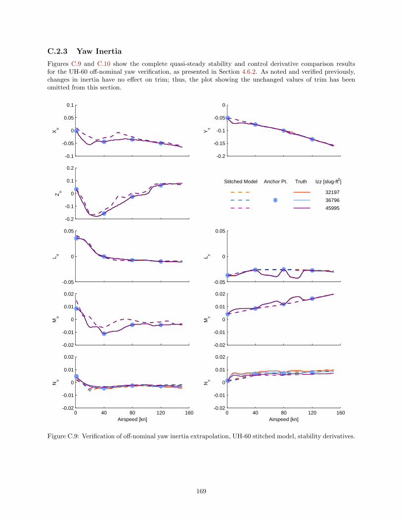
C.2.3 Yaw Inertia

Figures C.9 and C.10 show the complete quasi-steady stability and control derivative comparison resultsfor the UH-60 off-nominal yaw verification, as presented in Section 4.6.2. As noted and verified previously,changes in inertia have no effect on trim; thus, the plot showing the unchanged values of trim has beenomitted from this section.

-0.1

-0.05

0

0.05

0.1

Xu

-0.2

-0.15

-0.1

-0.05

0

Yv

-0.2

-0.1

0

0.1

0.2

Zu

-0.05

0

0.05

L u

-0.05

0

0.05

L v

-0.02

-0.01

0

0.01

0.02

Mu

-0.02

-0.01

0

0.01

0.02

Mv

0 40 80 120 160-0.02

-0.01

0

0.01

0.02

Nu

Airspeed [kn]

0 40 80 120 160-0.02

-0.01

0

0.01

0.02

Nv

Airspeed [kn]

Stitched Model

32197

36796

45995


Figure C.9: Verification of off-nominal yaw inertia extrapolation, UH-60 stitched model, stability derivatives.

169

-0.05

0

0.05

Xw

0.5

1

1.5

2

Xq

-1

0

1

2

Yq

-0.8

-0.6

-0.4

-0.2

0

Zw

-3

-2

-1

0

1

Zq

0

0.01

0.02

0.03

0.04

L w

-0.5

0

0.5

1

1.5

L q

-0.02

-0.01

0

0.01

0.02

Mw

-2

-1.5

-1

-0.5

Mq

0 40 80 120 160-0.02

-0.01

0

0.01

0.02

Nw

Airspeed [kn]

0 40 80 120 160-0.5

0

0.5

1

Nq

Airspeed [kn]

Stitched Model

32197

36796

45995


Figure C.9: Verification of off-nominal yaw inertia extrapolation, UH-60 stitched model, stability derivatives(cont.)

170

-1

-0.5

0

0.5

1X

p

-2

-1

0

1

Xr

-1

-0.5

0

0.5

1

Yp

0

1

2

3

Yr

-2

0

2

4

Zp

0

1

2

3

Zr

-5

-4

-3

-2

L p

-0.2

0

0.2

0.4

0.6

L r

-0.4

-0.2

0

0.2

0.4

Mp

0 40 80 120 160-0.8

-0.6

-0.4

-0.2

0

Np

Airspeed [kn]

0 40 80 120 160-1.5

-1

-0.5

0

Nr

Airspeed [kn]

Stitched Model

32197

36796

45995


Figure C.9: Verification of off-nominal yaw inertia extrapolation, UH-60 stitched model, stability derivatives(cont.)

171

0

0.5

1

1.5

Xδ co

l

-1.6

-1.4

-1.2

-1

-0.8

Xδ lo

n

0.1

0.2

0.3

0.4

Yδ co

l

-8.5

-8

-7.5

-7

-6.5

Zδ co

l

-10

-5

0

Zδ lo

n

-0.2

0

0.2

0.4

0.6

L δ col

0

0.1

0.2

0.3

0.4

L δ lon

-0.1

0

0.1

0.2

0.3

Mδ co

l

0.4

0.5

0.6

0.7

Mδ lo

n

0 40 80 120 160-0.2

-0.1

0

0.1

0.2

Nδ co

l

Airspeed [kn]

0 40 80 120 160-0.03

-0.02

-0.01

0

0.01

Nδ lo

n

Airspeed [kn]

Stitched Model

32197

36796

45995


Figure C.10: Verification of off-nominal yaw inertia extrapolation, UH-60 stitched model, control derivatives.

172

-0.2

-0.1

0

0.1

0.2

Xδ la

t

0.5

1

1.5

2

Xδ pe

d

0.35

0.4

0.45

0.5

Yδ la

t

-1.6

-1.4

-1.2

-1

-0.8

Yδ pe

d

0

0.1

0.2

0.3

0.4

Zδ la

t

0

2

4

6

Zδ pe

d

0.5

1

1.5

L δ lat

-1

-0.8

-0.6

-0.4

-0.2

L δ ped

-0.02

0

0.02

0.04

Mδ la

t

0 40 80 120 1600.04

0.06

0.08

0.1

0.12

Nδ la

t

Airspeed [kn]

0 40 80 120 1600.2

0.4

0.6

0.8

1

Nδ pe

d

Airspeed [kn]

Stitched Model

32197

36796

45995


Figure C.10: Verification of off-nominal yaw inertia extrapolation, UH-60 stitched model, control derivatives(cont.)

173

C.3 Center of Gravity

The UH-60 stitched model was configured with off-nominal CG location values and verified against FORE-CAST point models. Section C.3.1 presents the results for off-nominal fuselage-station CG location, andSection C.3.2 presents the results for off-nominal buttline CG location.

C.3.1 Station CG

Figures C.11–C.13 show the complete trim and quasi-steady stability and control derivative verificationresults for the UH-60 stitched model configured with fuselage-station CG location (x-body axis, positive aft)offsets, as discussed in Section 4.6.3.

2

4

6

8

δ col [i

n]

3

4

5

6

δ lon [i

n]

4

4.5

5

5.5

6

δ lat [i

n]

0 40 80 120 1601

2

3

4

δ ped [i

n]

Airspeed [kn]

-10

-5

0

5

10θ

[deg

]

-3

-2

-1

0

1

φ [d

eg]

0 40 80 120 160-1

-0.5

0

0.5

1

β [d

eg]

Airspeed [kn]

Stitched Model

355

358

361


Figure C.11: Verification of off-nominal station CG extrapolation, UH-60 stitched model, trim.

174

-0.1

-0.05

0

0.05

0.1

Xu

-0.1

-0.05

0

0.05

0.1

Xv

-0.1

-0.05

0

0.05

0.1

Yu

-0.2

-0.15

-0.1

-0.05

0

Yv

-0.2

-0.1

0

0.1

0.2

Zu

-0.05

0

0.05

L u

-0.05

0

0.05

L v

-0.02

-0.01

0

0.01

0.02

Mu

-0.02

-0.01

0

0.01

0.02

Mv

0 40 80 120 160-0.02

-0.01

0

0.01

0.02

Nu

Airspeed [kn]

0 40 80 120 160-0.02

-0.01

0

0.01

0.02

Nv

Airspeed [kn]

Stitched Model

355

358

361


Figure C.12: Verification of off-nominal station CG extrapolation, UH-60 stitched model, stability deriva-tives.

175

-0.05

0

0.05

Xw

0.5

1

1.5

2

Xq

-1

0

1

2

Yq

-0.8

-0.6

-0.4

-0.2

0

Zw

-4

-2

0

2

Zq

0

0.01

0.02

0.03

0.04

L w

-0.5

0

0.5

1

1.5

L q

-0.01

-0.005

0

0.005

0.01

Mw

-2

-1.5

-1

-0.5

Mq

0 40 80 120 160-0.01

-0.005

0

0.005

0.01

Nw

Airspeed [kn]

0 40 80 120 160-0.5

0

0.5

1

Nq

Airspeed [kn]

Stitched Model

355

358

361


Figure C.12: Verification of off-nominal station CG extrapolation, UH-60 stitched model, stability derivatives(cont.)

176

-1

-0.5

0

0.5

1X

p

-2

-1

0

1

Xr

-1

-0.5

0

0.5

1

Yp

0

1

2

3

Yr

-2

0

2

4

Zp

0

1

2

3

Zr

-5

-4

-3

-2

L p

-0.2

0

0.2

0.4

0.6

L r

-0.4

-0.2

0

0.2

0.4

Mp

0 40 80 120 160-0.8

-0.6

-0.4

-0.2

0

Np

Airspeed [kn]

0 40 80 120 160-1

-0.8

-0.6

-0.4

-0.2

Nr

Airspeed [kn]

Stitched Model

355

358

361


Figure C.12: Verification of off-nominal station CG extrapolation, UH-60 stitched model, stability derivatives(cont.)

177

0

0.5

1

1.5

Xδ co

l

-1.6

-1.4

-1.2

-1

-0.8

Xδ lo

n

0.1

0.2

0.3

0.4

Yδ co

l

-8.5

-8

-7.5

-7

-6.5

Zδ co

l

-10

-5

0

Zδ lo

n

-0.2

0

0.2

0.4

0.6

L δ col

-0.1

0

0.1

0.2

0.3

L δ lon

-0.1

0

0.1

0.2

0.3

Mδ co

l

0.4

0.5

0.6

0.7

Mδ lo

n

0 40 80 120 160-0.5

0

0.5

Nδ co

l

Airspeed [kn]

0 40 80 120 160-0.5

0

0.5

Nδ lo

n

Airspeed [kn]

Stitched Model

355

358

361


Figure C.13: Verification of off-nominal station CG extrapolation, UH-60 stitched model, control derivatives.

178

-0.2

-0.1

0

0.1

0.2

Xδ la

t

0.5

1

1.5

2

Xδ pe

d

0.35

0.4

0.45

0.5

Yδ la

t

-1.6

-1.4

-1.2

-1

-0.8

Yδ pe

d

-0.1

0

0.1

0.2

0.3

Zδ la

t

0

2

4

6

Zδ pe

d

1

1.1

1.2

1.3

1.4

L δ lat

-1

-0.8

-0.6

-0.4

-0.2

L δ ped

-0.02

0

0.02

0.04

Mδ la

t

0 40 80 120 1600.06

0.07

0.08

0.09

Nδ la

t

Airspeed [kn]

0 40 80 120 160

0.4

0.5

0.6

0.7

Nδ pe

d

Airspeed [kn]

Stitched Model

355

358

361


Figure C.13: Verification of off-nominal station CG extrapolation, UH-60 stitched model, control derivatives(cont.)

179

C.3.2 Buttline CG

Figures C.14–C.16 show the complete trim and quasi-steady stability and control derivative verificationresults for the UH-60 stitched model configured with a buttline CG location (y-body axis, positive right)offset, as discussed in Section 4.6.3.

2

4

6

8

δ col [i

n]

3

4

5

6

δ lon [i

n]

2

3

4

5

6

δ lat [i

n]

0 40 80 120 1601

2

3

4

δ ped [i

n]

Airspeed [kn]

-5

0

5

10

θ [d

eg]

-4

-2

0

2

4

φ [d

eg]

0 40 80 120 160-1

-0.5

0

0.5

1

β [d

eg]

Airspeed [kn]

Stitched Model

0

6

Truth Buttline CG [in]Anchor Pt.

Figure C.14: Verification of off-nominal buttline CG extrapolation, UH-60 stitched model, trim.

180

-0.1

-0.05

0

0.05

0.1

Xu

-0.1

-0.05

0

0.05

0.1

Xv

-0.1

-0.05

0

0.05

0.1

Yu

-0.2

-0.15

-0.1

-0.05

0

Yv

-0.2

-0.1

0

0.1

0.2

Zu

-0.05

0

0.05

L u

-0.05

0

0.05

L v

-0.02

-0.01

0

0.01

0.02

Mu

-0.02

-0.01

0

0.01

0.02

Mv

0 40 80 120 160-0.02

-0.01

0

0.01

0.02

Nu

Airspeed [kn]

0 40 80 120 160-0.02

-0.01

0

0.01

0.02

Nv

Airspeed [kn]

Stitched Model

0

6


Figure C.15: Verification of off-nominal buttline CG extrapolation, UH-60 stitched model, stability deriva-tives.

181

-0.05

0

0.05

Xw

0.5

1

1.5

2

Xq

-1

0

1

2

Yq

-0.8

-0.6

-0.4

-0.2

0

Zw

-3

-2

-1

0

1

Zq

0

0.02

0.04

0.06

0.08

L w

-0.5

0

0.5

1

1.5

L q

-0.01

-0.005

0

0.005

0.01

Mw

-2

-1.5

-1

-0.5

Mq

0 40 80 120 160-0.01

-0.005

0

0.005

0.01

Nw

Airspeed [kn]

0 40 80 120 160-0.5

0

0.5

1

Nq

Airspeed [kn]

Stitched Model

0

6


Figure C.15: Verification of off-nominal buttline CG extrapolation, UH-60 stitched model, stability deriva-tives (cont.)

182

-1

-0.5

0

0.5

1X

p

-2

-1

0

1

Xr

-1

-0.5

0

0.5

1

Yp

0

1

2

3

Yr

-2

0

2

4

Zp

0

1

2

3

Zr

-5

-4

-3

-2

L p

-0.5

0

0.5

L r

-0.5

0

0.5

Mp

0 40 80 120 160-0.8

-0.6

-0.4

-0.2

0

Np

Airspeed [kn]

0 40 80 120 160-1

-0.8

-0.6

-0.4

-0.2

Nr

Airspeed [kn]

Stitched Model

0

6


Figure C.15: Verification of off-nominal buttline CG extrapolation, UH-60 stitched model, stability deriva-tives (cont.)

183

0

0.5

1

1.5

Xδ co

l

-1.6

-1.4

-1.2

-1

-0.8

Xδ lo

n

-0.2

0

0.2

0.4

0.6

Yδ co

l

-8.5

-8

-7.5

-7

-6.5

Zδ co

l

-10

-5

0

Zδ lo

n

-0.5

0

0.5

1

L δ col

0

0.2

0.4

0.6

0.8

L δ lon

-0.1

0

0.1

0.2

0.3

Mδ co

l

0.4

0.5

0.6

0.7

Mδ lo

n

0 40 80 120 160-0.2

-0.1

0

0.1

0.2

Nδ co

l

Airspeed [kn]

0 40 80 120 160-0.5

0

0.5

Nδ lo

n

Airspeed [kn]

Stitched Model

0

6


Figure C.16: Verification of off-nominal buttline CG extrapolation, UH-60 stitched model, control derivatives.

184

-0.2

-0.1

0

0.1

0.2

Xδ la

t

0.5

1

1.5

2

Xδ pe

d

0.35

0.4

0.45

0.5

Yδ la

t

-1.6

-1.4

-1.2

-1

-0.8

Yδ pe

d

0

0.1

0.2

0.3

0.4

Zδ la

t

0

2

4

6

Zδ pe

d

1

1.1

1.2

1.3

1.4

L δ lat

-1.2

-1

-0.8

-0.6

-0.4

L δ ped

-0.02

0

0.02

0.04

Mδ la

t

0 40 80 120 1600.06

0.07

0.08

0.09

Nδ la

t

Airspeed [kn]

0 40 80 120 160

0.4

0.5

0.6

0.7

Nδ pe

d

Airspeed [kn]

Stitched Model

0

6


Figure C.16: Verification of off-nominal buttline CG extrapolation, UH-60 stitched model, control derivatives(cont.)

185

C.4 Altitude

Figures C.17–C.19 show the complete trim and quasi-steady stability and control derivative comparisonresults for the UH-60 off-nominal altitude verification, as presented in Section 4.6.4.

2

4

6

8

10

δ col [i

n]

3

4

5

6

δ lon [i

n]

4

4.5

5

5.5

6

δ lat [i

n]

0 40 80 120 1601

2

3

4

δ ped [i

n]

Airspeed [kn]

-5

0

5

10

θ [d

eg]

-3

-2

-1

0

1

φ [d

eg]

0 40 80 120 160-1

-0.5

0

0.5

1

β [d

eg]

Airspeed [kn]

Stitched Model

0

3000

6000

10000


Figure C.17: Verification of altitude extrapolation, UH-60 stitched model, trim.

186

-0.1

-0.05

0

0.05

0.1

Xu

-0.1

-0.05

0

0.05

0.1

Xv

-0.1

-0.05

0

0.05

0.1

Yu

-0.2

-0.1

0

0.1

0.2

Yv

-0.2

-0.1

0

0.1

0.2

Zu

-0.05

0

0.05

L u

-0.05

0

0.05

L v

-0.02

-0.01

0

0.01

0.02

Mu

-0.02

-0.01

0

0.01

0.02

Mv

0 40 80 120 160-0.02

-0.01

0

0.01

0.02

Nu

Airspeed [kn]

0 40 80 120 160-0.02

-0.01

0

0.01

0.02

Nv

Airspeed [kn]

Stitched Model

0

3000

6000

10000


Figure C.18: Verification of altitude extrapolation, UH-60 stitched model, stability derivatives.

187

-0.05

0

0.05

Xw

0

1

2

3

Xq

-1

0

1

2

Yq

-0.8

-0.6

-0.4

-0.2

0

Zw

-4

-2

0

2

Zq

0

0.01

0.02

0.03

0.04

L w

-4

-2

0

2

L q

-0.02

-0.01

0

0.01

0.02

Mw

-2

-1.5

-1

-0.5

0

Mq

0 40 80 120 160-0.02

-0.01

0

0.01

0.02

Nw

Airspeed [kn]

0 40 80 120 160-0.5

0

0.5

1

Nq

Airspeed [kn]

Stitched Model

0

3000

6000

10000


Figure C.18: Verification of altitude extrapolation, UH-60 stitched model, stability derivatives (cont.)

188

-1

0

1

2X

p

-2

-1

0

1

Xr

-1

0

1

2

Yp

0

1

2

3

Yr

-2

0

2

4

Zp

0

1

2

3

Zr

-6

-5

-4

-3

-2

L p

-0.5

0

0.5

L r

-0.5

0

0.5

Mp

0 40 80 120 160-0.8

-0.6

-0.4

-0.2

0

Np

Airspeed [kn]

0 40 80 120 160-1

-0.8

-0.6

-0.4

-0.2

Nr

Airspeed [kn]

Stitched Model

0

3000

6000

10000


Figure C.18: Verification of altitude extrapolation, UH-60 stitched model, stability derivatives (cont.)

189

0

0.5

1

1.5

Xδ co

l

-1.6

-1.4

-1.2

-1

-0.8

Xδ lo

n

-0.1

0

0.1

0.2

0.3

Yδ co

l

-9

-8

-7

-6

-5

Zδ co

l

-10

-5

0

Zδ lo

n

-0.2

0

0.2

0.4

0.6

L δ col

-0.1

0

0.1

0.2

0.3

L δ lon

-0.2

-0.1

0

0.1

0.2

Mδ co

l

0.4

0.5

0.6

0.7

Mδ lo

n

0 40 80 120 160-0.1

0

0.1

0.2

0.3

Nδ co

l

Airspeed [kn]

0 40 80 120 160-0.5

0

0.5

Nδ lo

n

Airspeed [kn]

Stitched Model

0

3000

6000

10000


Figure C.19: Verification of altitude extrapolation, UH-60 stitched model, control derivatives.

190

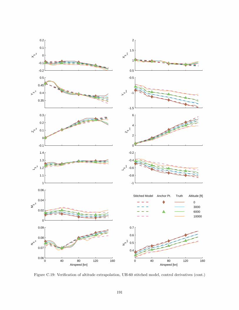
-0.2

-0.1

0

0.1

0.2

Xδ la

t

0.5

1

1.5

2

Xδ pe

d

0.35

0.4

0.45

0.5

Yδ la

t

-1.5

-1

-0.5

Yδ pe

d

-0.1

0

0.1

0.2

0.3

Zδ la

t

0

2

4

6

Zδ pe

d

1

1.1

1.2

1.3

1.4

L δ lat

-1

-0.8

-0.6

-0.4

-0.2

L δ ped

0

0.02

0.04

0.06

Mδ la

t

0 40 80 120 1600.06

0.07

0.08

0.09

Nδ la

t

Airspeed [kn]

0 40 80 120 160

0.4

0.5

0.6

0.7

Nδ pe

d

Airspeed [kn]

Stitched Model

0

3000

6000

10000


Figure C.19: Verification of altitude extrapolation, UH-60 stitched model, control derivatives (cont.)

191

C.5 Sling-Load Weight

Figures C.20–C.22 show the complete trim and quasi-steady stability and control derivative comparisonresults for the UH-60 with sling load verification, as presented in Section 4.8. Linear interpolation between(and extrapolation beyond) the trim data and dimensional stability and control derivatives of the twoanchor configurations within the stitched model was performed to simulate the alternate sling-load weightconfigurations.

4

5

6

7

δ col [i

n]

3.5

4

4.5

5

5.5

δ lon [i

n]

4

4.5

5

5.5

δ lat [i

n]

0 40 80 1201.5

2

2.5

3

3.5

δ ped [i

n]

Airspeed [kn]

-5

0

5

10

θ [d

eg]

-3

-2

-1

0

φ [d

eg]

0 40 80 120-1

-0.5

0

0.5

1

β [d

eg]

Airspeed [kn]

Stitched Model

0.1

0.15

0.2

0.27


Figure C.20: Alternate configuration verification, sling-load weight, UH-60 stitched model, trim.

192

-0.15

-0.1

-0.05

0

0.05

Xu

-0.2

-0.1

0

0.1

0.2

Xv

-0.1

-0.05

0

0.05

0.1

Yu

-0.4

-0.3

-0.2

-0.1

0

Yv

-0.2

-0.1

0

0.1

0.2

Zu

-0.05

0

0.05

L u

-0.05

0

0.05

L v

-0.02

-0.01

0

0.01

0.02

Mu

-0.02

-0.01

0

0.01

0.02

Mv

0 40 80 120-0.02

-0.01

0

0.01

0.02

Nu

Airspeed [kn]

0 40 80 120-0.02

-0.01

0

0.01

0.02

Nv

Airspeed [kn]

Stitched Model

0.1

0.15

0.2

0.27


Figure C.21: Alternate configuration verification, sling-load weight, UH-60 stitched model, stability deriva-tives.

193

-0.05

0

0.05

Xw

0

5

10

15

Xq

-1

0

1

2

Yq

-0.8

-0.6

-0.4

-0.2

0

Zw

-0.5

0

0.5

1

1.5

Zq

0

0.005

0.01

0.015

L w

-0.5

0

0.5

L q

-0.02

-0.01

0

0.01

0.02

Mw

-1.5

-1

-0.5

Mq

0 40 80 120-0.02

-0.01

0

0.01

0.02

Nw

Airspeed [kn]

0 40 80 120-0.5

0

0.5

1

Nq

Airspeed [kn]

Stitched Model

0.1

0.15

0.2

0.27


Figure C.21: Alternate configuration verification, sling-load weight, UH-60 stitched model, stability deriva-tives (cont.)

194

-4

-2

0

2X

p

-2

-1

0

1

Xr

-10

-8

-6

-4

Yp

0

1

2

3

Yr

-1

0

1

2

3

Zp

0

1

2

3

Zr

-2

-1.5

-1

-0.5

0

L p

-0.1

0

0.1

0.2

0.3

L r

-0.2

0

0.2

0.4

0.6

Mp

0 40 80 120-0.4

-0.3

-0.2

-0.1

0

Np

Airspeed [kn]

0 40 80 120-0.8

-0.6

-0.4

-0.2

0

Nr

Airspeed [kn]

Stitched Model

0.1

0.15

0.2

0.27


Figure C.21: Alternate configuration verification, sling-load weight, UH-60 stitched model, stability deriva-tives (cont.)

195

-1

0

1

2X

δ col

-6

-5

-4

-3

-2

Xδ lo

n

-0.5

0

0.5

1

Yδ co

l

-8

-7

-6

-5

-4

Zδ co

l

-6

-4

-2

0

Zδ lo

n

-0.1

0

0.1

0.2

0.3

L δ col

-0.1

0

0.1

0.2

0.3

L δ lon

-0.05

0

0.05

0.1

0.15

Mδ co

l

0.1

0.2

0.3

0.4

0.5

Mδ lo

n

0 40 80 120-0.2

-0.1

0

0.1

0.2

Nδ co

l

Airspeed [kn]

0 40 80 120-0.1

0

0.1

0.2

0.3

Nδ lo

n

Airspeed [kn]

Stitched Model

0.1

0.15

0.2

0.27


Figure C.22: Alternate configuration verification, sling-load weight, UH-60 stitched model, control deriva-tives.

196

-0.4

-0.3

-0.2

-0.1

0

Xδ la

t

0.5

1

1.5

2

Xδ pe

d

2

2.5

3

3.5

Yδ la

t

-3

-2.5

-2

-1.5

-1

Yδ pe

d

0.05

0.1

0.15

0.2

0.25

Zδ la

t

0

2

4

6

Zδ pe

d

0

0.5

1

L δ lat

-1

-0.5

0

L δ ped

-0.02

0

0.02

0.04

Mδ la

t

0 40 80 1200.03

0.04

0.05

0.06

Nδ la

t

Airspeed [kn]

0 40 80 1200

0.5

1

Nδ pe

d

Airspeed [kn]

Stitched Model

0.1

0.15

0.2

0.27


Figure C.22: Alternate configuration verification, sling-load weight, UH-60 stitched model, control derivatives(cont.)

197

References

[1] Tischler, M. B., Aircraft and Rotorcraft System Identification: Engineering Methods with Flight TestExamples, American Institute of Aeronautics and Astronautics, Inc., Reston, VA, 2nd ed., 2012.

[2] Marcos, A. and Balas, G. J., “Development of Linear-Parameter-Varying Models for Aircraft,” AIAAJournal of Guidance, Control, and Dynamics, Vol. 27, No. 2, March–April 2004.

[3] Aiken, E. W., “A Mathematical Representation of an Advanced Helicopter for Piloted Simulator In-vestigations of Control-System and Display Variations,” NASA TM 81203, AVRADCOM TM 80-A-2,July 1980.

[4] Tischler, M. B., “Aerodynamic Model for Piloted V/STOL Simulation,” Systems Technology, Inc., WP1171-2, Hawthorne, CA, May 1982.

[5] Zivan, L. and Tischler, M. B., “Development of a Full Flight Envelope Helicopter Simulation UsingSystem Identification,” Journal of the American Helicopter Society , Vol. 55, No. 022003, 2010, pp. 1–15.

[6] Lawrence, B., Malpica, C. A., and Theodore, C. R., “The Development of a Large Civil TiltrotorSimulation for Hover and Low-Speed Handling Qualities Investigations,” 36th European RotorcraftForum, Paris, France, September 2010.

[7] Mansur, M. H., Tischler, M. B., Bielefield, M. D., Bacon, J. W., Cheung, K. K., Berrios, M. G.,and Rothman, K. E., “Full Flight Envelope Inner-Loop Control Law Development for the UnmannedK-MAX,” American Helicopter Society 67th Annual Forum, Virginia Beach, VA, May 2011.

[8] Downs, J., Prentice, R., Dalzell, S., Besachio, A., Ivler, C. M., Tischler, M. B., and Mansur, M. H.,“Control System Development and Flight Test Experience with the MQ-8B Fire Scout Vertical Take-Off Unmanned Aerial Vehicle (VTUAV),” American Helicopter Society 63rd Annual Forum, VirginiaBeach, VA, May 2007.

[9] Greiser, S. and Seher-Weiss, S., “A contribution to the development of a full flight envelope quasi-nonlinear helicopter simulation,” CEAS Aeronautical Journal , Vol. 5, No. 1, March 2014, pp. 53–66.

[10] Spires, J. M. and Horn, J. F., “Multi-Input Multi-Output Model-Following Control Design Methods forRotorcraft,” American Helicopter Society 71st Annual Forum, Virginia Beach, VA, May 2015.

[11] McRuer, D., Ashkenas, I., and Graham, D., Aircraft Dynamics and Automatic Control , PrincetonUniversity Press, Princeton, NJ, 1973.

[12] MATLAB version 7.14.0.739 (R2012a), The MathWorks, Inc., Natick, MA, 2012.

[13] Stevens, B. L. and Lewis, F. L., Aircraft Control and Simulation, John Wiley & Sons, Inc., Hoboken,NJ, 2nd ed., 2003.

[14] Anon., “Flying Qualities of Piloted Aircraft,” MIL-STD-1797B, Department of Defense Interface Stan-dard, February 2006.

[15] Lusardi, J. A., von Gruenhagen, W., and Seher-Weiss, S., “Parametric Turbulence Modeling for Rotor-craft Applications – Approach, Flight Tests and Verification,” Proceedings of the Rotorcraft HandlingQualities Conference, November 2008.

[16] Roskam, J., Malaek, S., Anemaat, W., and Gerren, D., “Advanced Aircraft Analysis: A User FriendlyApproach to Preliminary Design and Analysis,” Proceedings of the AIAA Techfest XVI , November 1989.

199

[17] Tobias, E. L., Tischler, M. B., Berger, T., and Hagerott, S. G., “Full Flight-Envelope Simulation andPiloted Fidelity Assessment of a Business Jet Using a Model Stitching Architecture,” AIAA Modelingand Simulation Technologies Conference, Kissimmee, FL, January 2015.

[18] Anon., “U.S. Naval Test Pilot School Flight Test Manual – Fixed Wing Stability and Control Theoryand Flight Test Techniques,” USNTPS-FTM-No. 103, Naval Air Warfare Center, Aircraft Division,Patuxent River, MD, January 1997.

[19] Roskam, J., Airplane Design, Roskam Aviation and Engineering Corporation, Ottawa, KS, 1985.

[20] Kim, F. D., Celi, R., and Tischler, M. B., “High-Order State Space Simulation Models of HelicopterFlight Mechanics,” Journal of the American Helicopter Society , Vol. 38, No. 4, October 1993, pp. 16–27.

[21] Howlett, J. J., “UH-60A Black Hawk Engineering Simulation Program: Volume I – MathematicalModel,” NASA CR-166309, December 1981.

[22] Lusardi, J. A., Blanken, C. L., Braddom, S. R., Cicolani, L. S., and Tobias, E. L., “Development ofExternal Load Handling Qualities Criteria for Rotorcraft,” American Helicopter Society 66th AnnualForum, Phoenix, AZ, May 2010.

[23] Cooke, A. K. and Fitzpatrick, E. W., Helicopter Test and Evaluation, American Institute of Aeronauticsand Astronautics, Inc., Reston, VA, 2002.

200

a model stitching architecture for continuous full …

Documents