a model of the natural rate of unemployment and the
TRANSCRIPT

1
A Model of the Natural Rate of Unemployment and the Phillips Curve with Efficiency
Wages, Bargaining, and Search and Matching
Carl M. Campbell III
Department of Economics
Northern Illinois University
DeKalb, IL 60115
U.S.A.
815-753-6974
October 2017
Abstract
This paper develops a model of wage setting that combines efficiency wages, bargaining, and
search and matching. The model’s equilibrium conditions determine the economy’s natural rate of
unemployment. It is demonstrated that the natural rate depends positively on workers’ bargaining
power, the responsiveness of workers’ efficiency to their wages, unemployment benefits, the cost
of maintaining a vacancy, and the separation rate, and that it depends negatively on the efficiency
of matching. Expanding the model around its steady state yields an equation for the wage-wage
Phillips curve, in which wage inflation depends negatively on current unemployment, positively
on lagged unemployment (with the sum of coefficients on current and lagged unemployment being
negative), positively on expected future wage inflation, and positively on lagged wage inflation.
The model also yields an expression for the upward-sloping counterpart to the Phillips curve,
referred to as the Dynamic Labor Demand (DLD) curve. In the DLD curve, wage inflation depends
positively on the changes in the unemployment rate, the money supply, expected future real
demand, real interest rates, and expected price inflation. In addition, wage inflation depends
negatively on the change in technology in the DLD curve. (Wage inflation also depends on the
lagged change in the unemployment rate, but the effect is ambiguous.) Shifts of the Phillips curve
and DLD curve show the path of wage inflation and unemployment in response to macroeconomic
shocks (e.g., shocks to real aggregate demand, monetary growth, and technology). Empirical tests
with U.S. data find strong support for the model’s predictions, as all the coefficients in the Phillips
curve and DLD curve have the predicted sign, and most are significant at the 1% level.
Keywords: Natural rate; Phillips curve; Efficiency wage; Bargaining; Search and matching
JEL codes: E24; E31; J64

1
A Model of the Natural Rate of Unemployment and the Phillips Curve with Efficiency
Wages, Bargaining, and Search and Matching
1. Introduction
This study develops a model of the labor market that combines efficiency wage setting,
bargaining, and search and matching. From the model’s steady-state conditions, an equation is
derived that determines the economy’s natural rate of unemployment. This equation shows how
the natural rate is affected by changes in workers’ bargaining power, the responsiveness of
workers’ efficiency to their wages, unemployment benefits, the probability of a separation, the cost
of maintaining a vacancy, and the efficiency of the matching process.
The model is then expanded around its steady-state equilibrium, yielding an equation for
the wage Phillips curve, in which wage inflation depends positively on expected future wage
inflation and lagged wage inflation, depends negatively on the current unemployment rate, and
depends positively on lagged unemployment. In the Phillips curve, the sum of the coefficients on
current and lagged unemployment is negative. The slope of the Phillips curve depends on the
model’s microeconomic parameters, such as worker’s bargaining power, the separation rate, the
cost of a vacancy, the efficiency of matching, and the probability that a firm can adjust its wage.
In addition, the same framework is used to derive the upward-sloping counterpart to the Phillips
curve, referred to as the Dynamic Labor Demand (DLD) curve. In the DLD curve, wage inflation
depends positively on the changes the money supply, expected future real demand, real interest
rates, and expected price inflation, and wage inflation depends negatively on the change in
technology. In addition, wage inflation depends positively on the current change in the

2
unemployment rate, and it also depends on the lagged change in the unemployment rate, although
the effect is ambiguous.
The intersection of the Phillips curve and the DLD curve determines the economy’s
unemployment rate and rate of wage inflation. The Phillips curve – DLD framework can be used
to show the adjustment path the economy follows in the transition from its initial equilibrium to
its new equilibrium in response to shocks to productivity, real demand, and monetary policy.
The Phillips curve and DLD curve are simultaneously estimated with U.S. macroeconomic
data, and the empirical results strongly support the predictions of the theoretical model. The
coefficients in the Phillips curve and the DLD curve always have the expected sign and are usually
significant at the 1% level. In the DLD curve, 90% of the coefficients are significant at the 1%
level. In the Phillips curve, the coefficients on current unemployment, expected future wage
inflation, and lagged wage inflation are always significant at the 10% level, and 67% are significant
at the 1% level. In addition, the empirical results support the model’s predictions that the sum of
the coefficients on current and lagged unemployment is negative in the Phillips curve, but equals
0 in the DLD curve. Also, the model predicts that the coefficient on the money supply in the DLD
curve should equal the ratio over the sample period between changes in workers’ hourly wages
and nominal GDP per worker (approximately 0.85), and this prediction is supported by the
empirical results.
2. Assumptions
In deriving the model, the following assumptions are made:
1. There are a fixed number of workers in the economy, each of whom inelastically supplies
one unit of labor.
2. In each period a proportion, q, of workers separate from their jobs.

3
3. The utility of an individual worker (with subscript i denoting individual workers) when he
or she is employed can be expressed as
)( ,,, titi
E
ti eGWU ,
where )( ,tieG represents the disutility of providing effort when working. Workers provide
effort up to the point where the marginal disutility of providing effort equals the expected
value of keeping their job. Thus, thus disutility of effort should be proportional to the
average wage, so that utility can be expressed as,
ttiti
E
ti WegWU )( ,,, , (1)
where W represents the average wage in the economy.
4. A worker’s utility when unemployed is
titi
UN
ti BU ,,, ,
where is the value of leisure and B represents unemployment benefits. Both are assumed
to be proportional to the average wage,1 so that
t
UN
ti WbU )( *
, . (2)
5. Workers’ efficiency is described by the effort model of Campbell (2006), so that efficiency
can be expressed as
,0 ,0,0,0with)](,/[ WhWWhWttt eeeeuhWWee (3)
where h is the probability of an unemployed worker being hired, which depends negatively
on the unemployment rate (u). In Campbell (2006), the unemployment rate affects effort

4
indirectly through its effect on the hiring rate, since the cost of losing one’s job depends on
the probability of finding a new job if dismissed, which depends on the hiring rate rather
than on the unemployment rate, per se. Also, in the turnover cost models of Stiglitz (1974),
Schlicht (1978), and Salop (1979), the propensity to quit should depend on the probability
of finding another job.2 In addition, Section 3 shows that the equilibrium hiring rate is less
affected by changes in the separation rate as compared to the equilibrium unemployment
rate, making the equilibrium hiring rate more stable over time.
6. Firms produce output (Q) with the Cobb-Douglas production function,
)(1
ttttttt uh,W/WeKLAQ , (4)
where A represents technology (assumed to be labor augmenting), L is employment, K is
the capital stock, and represents the elasticity of output with respect to labor input, which
equals labor’s share of national income.
7. Firms face a downward-sloping demand curves for the good they produce,
t
tt
D
tP
PYQ (5)
where Y is real demand per firm, P is the price of the firm’s output, and P is the aggregate
price level.
8. When a job opening is vacant, the firm incurs a cost of Wc per unit time, where W is the
average wage. It is assumed that the cost is proportional to the average wage, since most
of the costs involved with recruiting new workers are labor costs.
9. The matching function can be expressed by the Cobb-Douglas function,

5
a
t
a
tt vum 1,
where u is the unemployment rate, v is the vacancy rate, and measures the efficiency of
matching.3 Let the represent the ratio between vacancies and unemployment. Then, the
probability of a firm filling a vacancy is
a
t
t
tt
v
m ,
and the probability of an unemployed worker being hired is
a
t
t
tt
u
mh 1 . (6)
10. Firms incur a fixed cost of operating. Thus, there are a finite number of firms, with the
number of firms determined by this cost. It is assumed that N represents the ratio between
workers and firms.
11. The workers at a firm are represented by a union, and the wage is determined from
bargaining between firms and the union to maximize
))(1()( tttt UU , (7)
where represents workers’ bargaining power, U* is the expected utility of workers in the
union, U is the reservation utility of workers in the union, is the firm’s profits, and
is the reservation level of profits. The reservation level of profits is assumed to be 0. In
addition, in line with Layard, Nickell, and Jackman (1991), it is assumed that the union’s
objective function is the fraction of the bargaining unit that is employed at the firm times
the utility of these workers plus the fraction of workers who are not employed at the firm
times the expected utility of these workers. Also, as in Layard, Nickell, and Jackman, it is

6
assumed that the union’s per-worker reservation level of utility equals the utility of an
unemployed individual.
12. Following the derivation in Romer (2012), aggregate demand is determined from the New
Keynesian IS-LM system described by
IS: 1
11
)1(
ttt YrY , and (8a)
LM:
1
1
t
t
t
t
t
i
iY
P
M,4 (8b)
where Y is real output, is the discount factor, r is the real interest rate, M is the money
supply, and i is the nominal interest rate.
13. Wage setting follows a Calvo (1983) process in which each period a fraction, , of firms
adjust their nominal wages to their optimal levels.
14. There is nominal inertia in wage setting. Two alternative ways to motivate this nominal
inertia are to assume that firms not optimizing their wages index them to lagged wage
inflation or to assume that firms’ expectations of future wage inflation are a mixture of
rational and adaptive expectations. While these assumptions are observationally
equivalent, this study makes the latter assumption because it is supported by the findings
of Fuhrer (1997), Roberts (1997), Pfajfar and Santoro (2010), and Levine et al. (2012),
whereas there appears to be little empirical evidence for the assumption of non-optimizing
firms to index their wages to lagged wage inflation. Accordingly, it is assumed that
])[1( 123121
,
1
,
1
w
TtT
w
t
w
t
w
t
uew
t
ew
t , (9)

7
where uew
t
,
1 represents firms’ unbiased expectations of future average wages, represents
the degree of rational expectations, 1- represents the degree of adaptive expectations, and
the ’s represent the weight placed on each lag in the adaptive component.
3. The Natural Rate of Unemployment
We first consider a steady state, in which all variables are constant. Because all variables
are constant, the time subscripts can be suppressed.
Behavior of Firms
From (5), a firm’s total revenues can be expressed as
PQYPQ
11
.
An equation for the present value of profits is determined from the framework of Pissarides
(2000) for large firms. Accordingly, can be expressed as
dtKPKPVWcWLPuhWWeKLAYe KKrt
0
11
1
)](,/[
(10a)
subject to the constraint,
qLVL a .5 (10b)
In the above equation, r is the real interest rate, PK is the price of capital goods, and is the
depreciation rate of capital.
The Appendix demonstrates that if the derivative of the profit function with respect to K is
set equal to zero, KP is set equal to P , and the resulting equation is solved for K, the optimal
capital stock is,

8
1
)1(
1
)1(
1
)1(
1
1
11
)](,/[)()1)(1(
uhWWeLAYrK . (11)
Substituting this value of K back into the original profit function yields
dtVWcWLr
rPuhWWeLAYe rt
)1(
)1)(1(
)()](,/[
1
)1)(1(
1
)1)(1(
0
1
)1(
1
)1(
1
)1(
1
1
(12a)
s.t. qLVL a . (12b)
Differentiating (12) with respect to L yields two first-order conditions,
0
)()](,/[1
)1( 1
)1)(1(
1
)1(1
1
)1(
1
)1(
1
1
dt
dxqx
WDrPuhWWeLAYe rt
(13a)
and
0 xWce art , (13b)
where
rD
)1(
)1)(1(
1
)1)(1(
.
From (13a) and (13b), the Appendix demonstrates that employment can be expressed as,
9
.)(
)](,/[)1(
1
)1)(1(1
)1()1(1
11
rP
uhWWeYADWcqr
WL a
(14)
The Appendix also demonstrates that substituting (14) into (12a) results in the following
expression for the profit function:
.)1(
1
)1(
1)()](,/[
1
1)1(
1
1
)1)(1(1)1(1(
Wcqr
WWcq
WWcqr
W
DrPuhWWeYAr
aaa
(15)
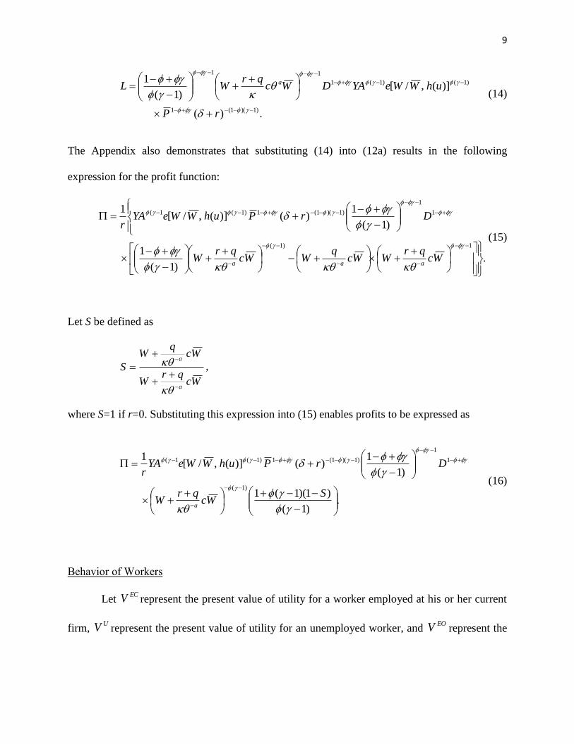
Let S be defined as
Wcqr
W
Wcq
W
S
a
a
,
where S=1 if r=0. Substituting this expression into (15) enables profits to be expressed as
.)1(
)1)(1(1
)1(
1)()](,/[
1
)1(
1
1
)1)(1(1)1(1(
SWc
qrW
DrPuhWWeYAr
a
(16)
Behavior of Workers
Let ECV represent the present value of utility for a worker employed at his or her current
firm, UV represent the present value of utility for an unemployed worker, and
EOV represent the

10
present value of utility for a worker employed at another firm. Equilibrium is described by the
following flow conditions:
][)( UECEC VVqWegWrV , (17a)
][)( UEOEO VVqWegWrV , (17b)
and
])[()( UEOU VVuhWbrV . (17c)
The Appendix demonstrates that the expected utility of a worker employed at his or her
current firm is
UEC V
qr
q
qr
W
qr
WV
, (18)
where is the equilibrium value of g(e), and that the expected utility of an unemployed worker is
Wuhqrr
uhqbrbV U
)]([
)1)(()()(
. (19)
From Assumption 11, the union’s expected utility is
UEC VN
LNV
N
LU
,
where NL / is the fraction of the bargaining unit that is employed at the firm, and NLN /)( is
the fraction of workers who are not employed at the firm. The reservation level of utility is assumed
to equal the utility of an unemployed individual, so thatUVU
. Thus, the difference between
expected utility and reservation utility can be expressed as,
][ UECUUEC VVN
LVV
N
LNV
N
LUU
. (20)

11
The Appendix demonstrates that substituting (18) and (19) into (20), and then substituting
(14) into the resulting expression yields
,)]()[(
)()(
],/[)1(
11
)1)(1(1
)1(1(1
11
Wuhqrqr
uhbqbr
qr
WrP
uWWeYADWcqr
WN
UUa
(21)
where *bb .
From Assumption 11, the wage is chosen to maximize equation (7). The Appendix
demonstrates that assuming that 0 and substituting (16) and (21) into (7) and maximizing the
resulting expression yields the equation,
)(
)(
)(
)(
)1()(
)(
)](,/[)](,/[ 1
uhqr
uhbqbr
W
Wc
qr
W
W
cqr
uhqr
uhbqbr
uhqr
uhbqbr
W
W
uhWWeuhWWe
a
a
W
. (22)
In equilibrium, the condition that separations equal new hires implies that
u
uquh
)1()(
. (23)
In addition, (6) and (23) imply that the equilibrium value of is
a
aaa
u
uqh
1
1
1
1
1
1
1
1)1(
. (24)
The Appendix demonstrates that setting W equal to W in (22) and substituting (23) and (24) into
the resulting expression yields the equilibrium condition:
12
.
)1()(1
)1()1(
)1(
)1)(1(1
)1(,1
)1(,1
11
1
11
1
1
a
a
a
a
a
a
W
u
uqcqr
u
uqc
u
uqqr
qr
u
uq
bb
u
uqe
u
uqe
(25)
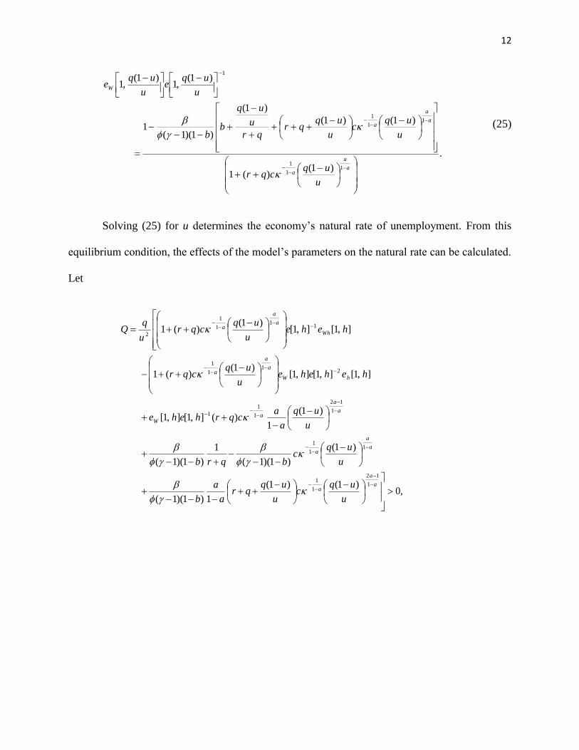
Solving (25) for u determines the economy’s natural rate of unemployment. From this
equilibrium condition, the effects of the model’s parameters on the natural rate can be calculated.
Let
,0)1()1(
1)1)(1(
)1(
)1)(1(
1
)1)(1(
)1(
1)(],1[],1[
],1[],1[],1[)1(
)(1
],1[],1[)1(
)(1
1
12
1
1
11
1
1
12
1
1
1
21
1
1
11
1
1
2
a
a
a
a
a
a
a
a
aW
hW
a
a
a
Wh
a
a
a
u
uqc
u
uqqr
a
a
b
u
uqc
bqrb
u
uq
a
acqrhehe
heheheu
uqcqr
heheu
uqcqr
u

13
,0)1()1()1(
1)1)(1(
)1()1(
)1)(1(
)1(
)1)(1()(
)1(
)1)(1(
)1(],1[],1[],1[
)1()(1
)1(],1[],1[
)1()(1
)1()1()(
1],1[],1[
)1(],1[],1[
1
12
1
1
11
1
11
1
2
21
1
1
11
1
1
1
12
1
1
1
11
1
1
u
u
u
uqc
u
uqqr
a
a
b
u
u
u
uqc
b
u
uqc
buqr
ur
b
u
uhehehe
u
uqcqr
u
uhehe
u
uqcqr
u
u
u
uqcqr
a
ahehe
u
uqcheheR
a
a
a
a
a
a
a
a
a
hW
a
a
a
Wh
a
a
a
a
a
aW
a
a
aW
and
0)1()1(
)(
)1( 11
1
a
a
a
u
uqc
u
uqqr
uqr
uqbZ .
Then, the Appendix demonstrates that
0)1)(1(
Q
b
Z
d
du
,
,0)1)(1(
)1(2
Q
b
bZ
db
du

14
,0
)1()1(
)1)(1()(],1[],1[
11
1
1
Q
u
uq
u
uqqr
bqrhehe
dc
du
a
a
aW
,0
)1(
)1)(1(
)1(
1
1)(
1],1[],1[
11
2
1
Q
u
uqc
b
u
uqqr
aqr
a
ahehe
d
du
a
a
a
a
W
and
0Q
R
dq
du.
In addition, the effect of We (the derivative of efficiency with respect of the relative wage)
on the natural rate can also be calculated. Suppose efficiency is expressed as
]),(,/[ zuhWWe , with 0Wze , 0ze .
Thus, z is a shift variable that raises the derivative of efficiency with respect to the relative wage,
but that has a neutral effect on efficiency itself. Then the Appendix demonstrates that
0],,1[],,1[ 1
Q
zhezhe
dz
du Wz .
Thus, as workers’ efficiency becomes more responsive to their wages, the economy’s natural rate
increases. In efficiency wage models, efficiency is generally treated as a function of workers’ effort
and quit propensities. Thus, the above relationship implies that equilibrium unemployment should

15
be higher for subgroups of workers and for countries in which effort and quit propensities are
highly responsive to relative wages.
Overall, the above comparative statics show that the natural rate depends positively on
workers’ bargaining power (), the ratio between unemployment benefits and wages (b), the cost
of maintaining a vacancy (c), the separation rate (q), and the derivative of efficiency with respect
to the wage (We ), and it depends negatively on the efficiency of matching ().
Suppose that the economy is characterized by a pure efficiency wage model, with no
bargaining or search and matching, so that c=0 and =0. In this case,
],1[],1[],1[],1[],1[
)1(],1[],1[],1[
)1(],1[],1[
21
2
21
heheheheheu
qu
uhehehe
u
uhehe
dq
du
hWWh
hWWh
,
resulting in the relationship,
.1 uu
q
dq
du (26)
Thus, in a pure efficiency wage model, the elasticity of the unemployment rate with respect
to the separation rate equals 1 minus the natural rate of unemployment, so that the natural rate
moves almost one-for-one with the separation rate. Campbell and Duca (2008) demonstrate that
the U.S. natural rate does, in fact, appear to behave as predicted by (26). Shimer (2007) constructs
data on the separation rate, and Campbell and Duca (2008) adjust Shimer’s data for business cycle
fluctuations, and then smooth it with a Hodrick-Prescott filter, producing a cyclically-adjusted and
smoothed separation rate. They then calibrate a model with U.S. data from 1960-1970, so that the

16
average value of the model’s natural rate over this period is equal to the average value of the
Congressional Budget Office’s (CBO) estimate of the U.S. natural rate.
Using the relationship in (26), they use the model to simulate the economy’s natural rate
from 1960-2005, based on data on the percentage of workers under the age of 35 and the cyclically-
adjusted and smoothed separation rate. In addition, they also simulate the ratio between the average
duration of unemployment and the unemployment rate over the same period. The simulation
demonstrates that the model’s predicted natural rate and duration-unemployment ratio closely
track both the actual natural rate (based on the CBO’s estimates) and the duration-unemployment
ratio. They also find that, over the 1960-1991 period, changes in the separation rate based on
demographics alone can explain these variables. However, after 1991 there was a decrease in the
separation rate that cannot be explained by demographics alone, and the model needs to
incorporate this unexplained decrease in the separation rate to accurately track the natural rate and
the duration-unemployment ratio after 1991.6
The assumption that efficiency depends on the hiring rate, which is a function of the
unemployment rate, means that changes in the separation rate will have a much greater impact on
the equilibrium unemployment rate than on the equilibrium hiring rate, a prediction that is
supported by U.S. data. Equation (23) shows that a change in the economy’s equilibrium separation
rate changes results in a change in equilibrium unemployment, the equilibrium hiring rate, or some
combination of the two. Comparing the 1970-1990 period with the 1991-2007 period indicates that
changes in the separation rate have a much greater impact on the unemployment rate than on the
hiring rate. Between the 1970-1990 period and the 1990-2007 period, the U.S. economy’s
separation rate fell by 21%. In response, the unemployment rate declined 19%, and the hiring rate
declined 2%. (The reason for not also considering the 1960’s is that actual GDP appears to have

17
been above potential GDP for most of this decade, while the latter decades were characterized by
alternating inflationary and recessionary gaps.) Thus, it appears that almost all of the effect of the
fall in the separation rate was to change equilibrium unemployment, leaving the equilibrium hiring
rate relatively unaffected. Thus, it seems reasonable to model efficiency as a function of the hiring
rate instead of the unemployment rate itself.
4. The Phillips Curve and the Dynamic Labor Demand (DLD) Curve
The Phillips curve can be obtained from approximating the equation for the natural rate
around its steady-state equilibrium by totally differentiating this equation and dividing by the
original equation. While the time subscripts are dropped in deriving the economy’s natural rate,
they are needed to obtain an expression for the Phillips curve, since the Phillips curve is a
relationship over time between inflation and unemployment. With time subscripts, (22) can be
expressed as
t
t
t
t
a
t
t
at
t
t
t
t
t
ttttttW
hqr
hbqbr
W
Wc
qr
W
W
cqr
hqr
hbqbr
hqr
hbqbr
W
W
hWWehWWe
)1(],/[],/[ 1 . (27)
When modeling the natural rate, it is assumed that hires are equal to separations. However,
this is no long true when the economy is away from its long-run equilibrium. In this case, the
difference between hires and separations equals the change in employment, so that
NuNuNuqNuh ttttt )1()1()1( 1 .
Thus, the probability of a hire can be expressed as
t
tttt
u
uuuqh
1)1(
. (28)

18
Also, the vacancy-unemployment ratio () is related to the hiring rate through the expression,
a
tth 1 .
Solving the above equation for and substituting (28) into the resulting expression enables the
vacancy-unemployment ratio to be expressed as,
a
t
tttaat
at
u
uuuqh
1
1
11
1
1
1
1
1)1(
. (29)
The Appendix demonstrates that by substituting (28) and (29) into (27), taking total
derivatives, dividing by the original equation, assuming staggered wage setting (from assumption
13), and assuming mixed rational and adaptive expectations (from assumption 14), the Phillips
curve can be expressed as
143
1
12
,
11
tt
T
j
w
jtj
uew
t
w
t dudu , (30)
where 0)1(1 1
1
,
0)1(1
)1(
1
2
,
0])1(1)[1(
)]1(1[
1
3
E
,
0])1(1)[1(
)]1(1[
1
4
F
.
In (30), w
t represents the percentage change in nominal wages, and tdu represents the percentage-
point difference between the unemployment rate and the natural rate. The expressions for E and F

19
are very complex and are reported in the Appendix. In the Phillips curve, wage inflation depends
on expected future wage inflation and current wage inflation, with the sum approximately equal to
1, and exactly equal to 1 if =1. Wage inflation also depends negatively on the level of current
unemployment and depends positively on the level of lagged unemployment. The Appendix
demonstrates that 43 , so the sum of the coefficients on current and lagged unemployment is
unambiguously negative. In addition, while the model incorporates technology shocks, these
shocks do not appear in the Phillips curve, so there is no need to control for technology shocks in
estimating the Phillips curve. However, as discussed below, technology shocks do appear in the
DLD curve, so these shocks result in a movement along the Phillips curve.
Since current wage inflation is a function of unemployment and of both expected future
and lagged wage inflation, (30) is an equation for the wage-wage Phillips curve. However, when
economists estimate Phillips curves, the right-hand side variable is generally expected price
inflation rather than expected wage inflation. While expected price inflation is the independent
variable in the vast majority of Phillips curve studies, the right-hand side variable in Phelps’s
(1968) seminal paper is expected wage inflation, resulting in a wage-wage Phillips curve.7 In
addition, Perry (1978) and Campbell (2017) regress the change in average hourly earnings (AHE)
on the unemployment rate and on lagged values of either AHE, the change in the consumer price
index (CPI), or the change in private nonfarm GDP deflator (GDPD). Both studies find a higher
R2 and a sum of coefficients on lagged inflation that is closer to 1 with lagged AHE than with
lagged CPI or GDPD, suggesting that the wage inflation process may be described more accurately
by a wage-wage Phillips curve than by a wage-price Phillips curve.

20
The model developed in this study can also be used to derive the upward-sloping
counterpart to the Phillips curve. The DLD curve is derived in the Appendix, and it is demonstrated
that
).()(
)1()ˆˆ(
)ˆˆ()ˆˆ()()(
111
1121211
e
t
e
titt
r
tt
tttttttt
w
t
ddsdrdrs
YY
MMAAdudududu
(31)
In (31), variables with “^’s” over them (e.g., tM̂ ) represent percentage deviations from steady-
state values, while variables preceded by “d” (e.g., tdr ) represent percentage-point deviations from
steady-state values. Also, si is the absolute value of the semi-elasticity of money demand with
respect to nominal interest rates, is the ratio between si and the absolute value of the semi-
elasticity of aggregate spending with respect to real interest rates, and )]/(1[ rsr . Also, 1
and 2 are given by the expressions,
0)(
1)1()(1
))(1(
2
11
2
1
21
u
uqsees
u
uqee
u
a
uqsa
LhL
h
W
,
u
aas
u
ee Wh )]1/()[1(1
2 ,
where he is the derivative of efficiency with respect to the hiring rate, Ls represents the
relationship between percentage deviations in aggregate hours worked and percentage-point
deviations in the unemployment rate from their steady-state values, and Ws is defined in the
Appendix. In (31), the sign on 2 is theoretically ambiguous.
In the DLD curve, wage inflation depends positively on the current change in the
unemployment rate, the change in the money supply, the expected future change in demand, the
21
change in the real interest rate, and the change in expected price inflation. In addition, wage
inflation depends negatively on the change in technology and depends either positively or
negatively on the lagged change in the unemployment rate. While the prediction that wage inflation
depends negatively on technology shocks (which also means that technology shocks shift the DLD
to the right and thus raise unemployment) seems counterintuitive, these predictions are consistent
with Basu, Fernald, and Kimball’s (2006) findings that technological improvements initially result
in lower employment and slightly lower nominal wages. While the direct effect of positive
technology shocks is to initially reduce employment and nominal wages, these shocks should also
increase future demand growth ( tt YY ˆˆ1 ) by raising permanent income and the marginal product
of capital, which will positively affect future employment and nominal wages.
In the DLD curve, wage inflation depends on the current change in the unemployment rate
and on the lagged change in the unemployment rate. Thus, if tu , 1tu , and 2tu are entered as
separate variables, the sum of coefficients on these variables should equal 0, a hypothesis that is
tested in Section 5.
In (30) and (31), there are two relationships, the Phillips curve and the DLD curve, that
simultaneously determine the economy’s unemployment rate and the rate of wage inflation. The
Phillips curve is shifted by lagged wage inflation, expected future wage inflation, and lagged
unemployment. The DLD curve is shifted by changes in technology, the money supply, expected
future real demand, real interest rates, and expected inflation, along with the first and second
lagged values of the unemployment rate. The Phillips curve – DLD framework can be used to
show the transition path over time of unemployment and wage inflation in response to aggregate
shocks, most importantly shocks to technology, the money supply, and real demand.
22
5. Empirical Estimation of the Phillips Curve and the DLD Curve
This section presents estimates of the Phillips curve and the DLD curve. The growth rate
in wages ( w
t ) is measured by the percentage change in Average Hourly Earnings (AHE), a series
available since 1964, and dut is the deviation of the unemployment rate from the Congressional
Budget Office’s estimate of the natural rate. Because expected future wage inflation ( uew
t
,
1 ) may
be correlated with the error term in the Phillips curve, this variable is instrumented. To instrument
uew
t
,
1 , the DLD curve in levels8 in (31) is solved for dut, and the resulting expression is substituted
into (30), which produces a difference equation. The solution to the difference equation shows that
wage inflation depends on the current, lagged, and future values of variables in the DLD, except
for the unemployment rate. Thus, the set of instruments are the changes in the money supply (along
with changes in trend velocity), technology, real GDP, and real interest rates.9
In the DLD curve, technology is measured with the utilization-adjusted series on total
factor productivity maintained by the Federal Reserve Bank of San Francisco, based on the method
of Basu, Fernald, and Kimball (2006) as updated in Basu, Fernald, Fisher, and Kimball (2013).
However, these estimates exhibit a great deal of volatility on a quarter-to-quarter basis, so they
might not be an accurate measure of true technological change. The real cost of imported crude oil
(OilPrice) is also included to capture the effect of an additional type of supply shock. The measure
of the money supply is M2 per worker. To account for long-term changes in money demand, the
trend change in velocity, estimated with a Hodrick-Prescott filter with a smoothing parameter of
1600, is also included in the regressions. Expected future real GDP growth is unobserved, but is
instrumented with real net wealth per worker, the University of Michigan’s Index of Consumer
Expectations, and technology.10

23
The real interest rate is measured by the 3-month Treasury bill rate11 minus the percentage
change in the GDP deflator. Expected price inflation is measured by the Livingston series of
expectations of the GDP deflator, which is available since 1971. Including this variable may be
problematic since it is probably highly correlated with past and expected future wage inflation and
since it is not available for the entire sample period. In addition, it enters (31) only because it
represents the difference between nominal and real interest rates. Because of these potential issues,
regressions are estimated both with and without this variable.
From (31), the DLD depends positively on the change in unemployment from period t-1 to
t and on the change in unemployment from period t-2 to t-1. To examine whether the DLD does,
in fact, depend on the change in unemployment (as predicted), the regressions include tu , 1tu ,
and 2tu as separate variables (as opposed to the regressions including 1 tt uu and 21 tt uu ).
If the DLD does depend on the change in the unemployment rate, then the sum of the coefficients
on these three values of unemployment should equal 0.
Because future wage inflation and future aggregate demand are instrumented, the equations
are estimated with full information maximum likelihood (FIML). An alternative way to estimate
these equations is with generalized methods of moments (GMM). However, Campbell (2017)
shows that the coefficients in a Phillips curve regression are much more stable with FIML than
with GMM estimation. In addition, Lindé (2005) simulates macroeconomic data with known
parameters and estimates Phillips curves with this simulated data, and he finds that FIML
estimation results in coefficient estimates that are much closer to the true parameter values as
compared with GMM.
Equations are estimated both over the entire 1967:2-2017:1 sample period and with data
from 1967:2-2007:4, which excludes the Great Recession and the subsequent recovery. The reason

24
for estimating equations that exclude post-2007 data is that the adjustment to the 2008 recession
would likely have entailed notional nominal wage reductions for a significant number of workers.
If these reductions did not occur because of downward nominal wage rigidity, the estimated
coefficients in the Phillips curve and DLD curve may differ from what they would have been in
the absence of wage rigidity.
The results are presented in Table 1, with estimates over the 1967:2-2017:1 sample period
in the first two columns and estimates over the 1967:2-2007:4 sample period in the last two
columns. Twelve lags of wage inflation are included in the Phillips curve, and Table 1 reports the
value of the first lag, the sum of the 2nd through 4th lag, the sum of the 5th through 8th lag, and the
sum of the 9th through 12th lag. The equation for the DLD curve includes the current and two lagged
values of the unemployment rate. Eq. (31) predicts that the coefficient on the current
unemployment rate should be positive and that the sum of the coefficients on the current, first
lagged, and second lagged values should equal 0. Also included in the DLD equation are the
current and three lagged values of the changes in technology, the M2 money supply, trend velocity,
oil prices, instrumented future real GDP, real interest rates, and expected inflation (in two
columns), and the sum of these coefficients is reported in Table 1.12
In the Phillips curve, the coefficient on the current unemployment rate is always negative
and significant at the 10% level, and this coefficient is always significant at the 1% level with data
over the entire sample period. The coefficient on lagged unemployment is always positive, and is
significant at the 5% level with equations estimated over the entire sample period. As predicted,
the sum of the coefficients on current and lagged unemployment is negative, and the sum is
significantly different from 0 at the 5% level in all four columns and is significant at the 1% level
in three of the four columns.

25
In the regression with pre-2008 data, the sum of coefficients on the unemployment rate lies
between –0.0675 and –0.0722. These estimates are roughly consistent with Galí’s (2011) estimates
of the new Keynesian wage Phillips curve with quarterly data through the end of 2007 (with lagged
year-to-year price inflation as an independent variable), in which the sum of coefficients is –0.096
or –0.099, depending on the measure of wages.
In the DLD curve, equation (31) predicts that the coefficient on current unemployment
should be positive, although the signs on unemployment lagged 1 or 2 periods are ambiguous. In
addition, (31) predicts that the coefficients on oil prices, the money supply (as well as trend
velocity), future real GDP, real interest rates, and expected inflation should be positive, while the
coefficient on technology should be negative. In Table 1, all 30 coefficients have the predicted
sign, all are significant at the 10% level, and 27 are significant at the 1% level. Thus, the predictions
of the theoretical model are strongly supported by the empirical results with U.S. macroeconomic
data.
In addition, (31) implies three specific predictions concerning the coefficients in the DLD.
First, the model predicts that the sum of the coefficients on current unemployment and lagged
unemployment should equal 0. Second, the coefficient on the change in technology is predicted to
equal the negative of the coefficient on the change in real demand. Third, the coefficient on the
growth in the money supply (adjusted for changes in trend velocity) should equal 1. However,
labor’s share of national income fell over both the full sample period and the pre-2008 sample
period, so nominal wages grew more slowly than nominal GDP per worker. On average, the ratio
between the average rise in AHE and the average rise in nominal GDP per worker was 0.842 over
the pre-2008 sample period and 0.855 over the full sample period. If represents this ratio, then
the sum of the coefficients on monetary growth and trend velocity should equal .

26
The last three rows of Table 1 report Likelihood Ratio tests of these restrictions. The test
of the restriction that 021 ttt uuu can be rejected at the 10% level in only one column, and
the coefficient on current unemployment is always within 3% of the sum of coefficients of the first
and second lag of unemployment. The restriction that A=-Y cannot be rejected at even the 10%
level with pre-2008 data, but can be rejected at the 1% level over the entire sample period.
However, true technological change is unobservable, and the technology data used in the
regressions are quite volatile and may not reflect true exogenous changes in technology. Thus, the
rejection of this restriction over the entire sample period may be a result of the way technological
growth was estimated.
The restriction that the sum of coefficients on M2 growth and trend velocity equals can
never be rejected at even the 10% level. These results indicate that monetary growth (adjusted for
trend velocity) has the expected effect on nominal wage growth. Thus, in addition to all the
coefficients having the predicted signs, two of the three restrictions on the coefficients implied by
the theoretical model are supported by the empirical estimation, and the restriction that is rejected
over the entire sample period may be a result of measurement error.
The coefficient on future wage inflation lies between 0.304 and 0.417 in the regressions in
Table 1. These estimates of the degree of forward-looking expectations are similar to the findings
of Lindé (2005), which estimates a coefficient on forward-looking inflation of 0.282 to 0.457 in
the Phillips curve, and to those of Levine et al. (2012), which estimates the degree of rational vs.
adaptive expectations with, finding (with their best specification) that 17-25% of firms and 30-
34% of households have rational expectations.

27
6. Possible Extensions to the Model
With U.S. quarterly data from 1951-2003, Shimer (2005) calculates the standard deviation
of the unemployment rate, the vacancy rate, the vacancy-unemployment ratio, the job finding rate,
the separation rate, and the growth in labor productivity, and also calculates the correlations
between these variables. With a canonical search and matching model, he then simulates shocks
to productivity (which are assumed to represent demand shocks) and shocks to the separation rate.
He finds that, in response to these shocks, the standard deviations of these variables and the
correlations between these variables generally do not come close to matching their values with
actual data, and these statistical measures are often off by a factor of 10-20. The failure of the
canonical search and matching model to replicate U.S. labor market data has become known as the
“Shimer puzzle.”
The present study considers the joint determination of unemployment and wage inflation.
The model can also be extended to simultaneously consider the behavior of wage inflation,
unemployment, vacancies, and the hiring rate. The empirical results in Section 5 demonstrate that
the model does a good job of explaining the behavior of wage inflation and unemployment. In
addition, Campbell (2017) develops a pure efficiency wage model that is similar to the model in
the present study, but which does not incorporate bargaining and search and matching
considerations. It is demonstrated that this more parsimonious model can generate large and
persistent fluctuations in the unemployment rate in response to demand shocks. For example, a 5%
decrease in aggregate demand gradually raises the unemployment rate until it is 2.7% above the
natural rate eight quarters after the shock, with the unemployment rate then declining until it is
approximately equal to the natural rate after 20 quarters. In actual U.S. recessions over the sample
period, the time for unemployment to reach is peak value ranges from 3-10 quarters, and the time

28
for it to return to the natural rate is between 17-24 quarters, consistent with the predictions of the
model.
Given the model’s ability to explain unemployment and wage inflation dynamics, it is
possible that using the model to simulate the response of unemployment, vacancies, the vacancy-
unemployment ratio, and the hiring rate to exogenous shocks may result in predicted standard
deviations and correlations in these variables that are reasonably close to their actual standard
deviations and correlations, at least in comparison to the canonical search and matching model.
Also, in Shimer (2005) aggregate demand shocks are proxied by the change in productivity. In the
present study, aggregate demand and productivity shocks appear separately in the DLD curve, so
the labor market’s response to both types of shocks can be analyzed separately, as well as the
response to separation rate shocks. Thus, simulating the behavior of unemployment, vacancies, the
vacancy-unemployment ratio, and the hiring rate in the model developed in this study may be a
promising approach to try to replicate the statistical properties of labor market data.
7. Conclusion
This study develops a model of the economy that incorporates efficiency wages,
bargaining, and search and matching. An equation is derived that determines the economy’s
equilibrium unemployment rate (i.e., the natural rate of unemployment), and comparative statics
show how changes in workers’ bargaining power, the responsiveness of workers’ efficiency to
wages, the level of unemployment benefits, the cost of a vacancy, the efficiency of the matching
process, and the separation rate affect the natural rate.
Approximating the model around its steady-state equilibrium results in two dynamic
macroeconomic relationships. One is the wage-wage Phillips curve, in which wage inflation
depends on expected future wage inflation, lagged wage inflation, the current unemployment rate,

29
and the lagged unemployment rate, with the overall effect of unemployment being negative. The
second is the Dynamic Labor Demand (DLD) curve. In this relationship, wage inflation depends
on the current and lagged changes in the unemployment rate and on changes in technology, the
money supply, expected future real aggregate demand, the real interest rate, and expected price
inflation. The joint Phillips curve – DLD curve system can be used to show the behavior of wage
inflation and unemployment in the transition from the economy’s initial equilibrium to its new
equilibrium in response to exogenous aggregate shocks.
Empirical tests of the model with U.S. macroeconomic data show strong support for the
model’s predictions. All the coefficients in both the Phillips curve and the DLD curve have the
predicted sign, almost all are significant at the 10% level, and most are significant at the 1% level.
In addition, support is found for two specific predictions about the magnitude of the coefficients
in the DLD. The model predicts that the sum of coefficients on the current and lagged
unemployment rates equals 0 and that the coefficient on the money supply equals the ratio over
the sample period between changes in workers’ hourly wages and nominal GDP per worker, and
these restrictions generally cannot be rejected at even the 10% level.

30
Appendix
Derivation of (11):
Setting the derivative of (10a) with respect to K equal to 0 yields
0
)](,/[)1)(1(
)1(1
)1)(1()1()1(1
rtK
Krt
edt
dP
PVWcWLPuhWWeKLAYe
(A1)
Solving (A1) for the optimal capital stock yields
1
)1(
1
)1(
1
)1(
1
1
11
)](,/[)()1)(1(
uhWWeLAYrK . (A2)
Derivation of (14):
From (13a) and (13b),
0)()](,/[1
)1( 1
)1)(1(
1
)1(1
1
)1(
1
)1(
1
1
Wcqr
WDrPuhWWeLAYa
.)(
)](,/[)1(
1
)1)(1(1
)1()1(1
11
rP
uhWWeYADWcqr
WL a

31
Derivation of (15):
dtrPuWWeAYDWcqr
W
qWcW
DrPuWWerPuWWe
AYDWcqr
WAYe
tt
e
ttttat
a
tt
tt
e
tttt
e
tt
ttattt
rt
)1)(1(1)1()1(1
1
1
1
)1)(1(
1
)1(
1
)1)(1(
)1()
1
)1(
1
)1(
1
)1(
)1(
)1()1(
0
1
)1(
1
1
)(],/[
)1(
1
)(],/[)(],/[
)1(
1
222
22
dtWcqr
Wq
WcW
Wcqr
W
DrPuWWeYAe
at
a
tt
at
tt
e
ttt
rt
1
)1(
0
1
1
)1)(1(1)1()1(
)1(
1
)1(
1)(],/[
1)1(
1
1
)1)(1(1)1(1(
)1(
1
)1(
1)()](,/[
1
Wcqr
Wq
WcWWcqr
W
DrPuhWWeYAr
a
a
a
32
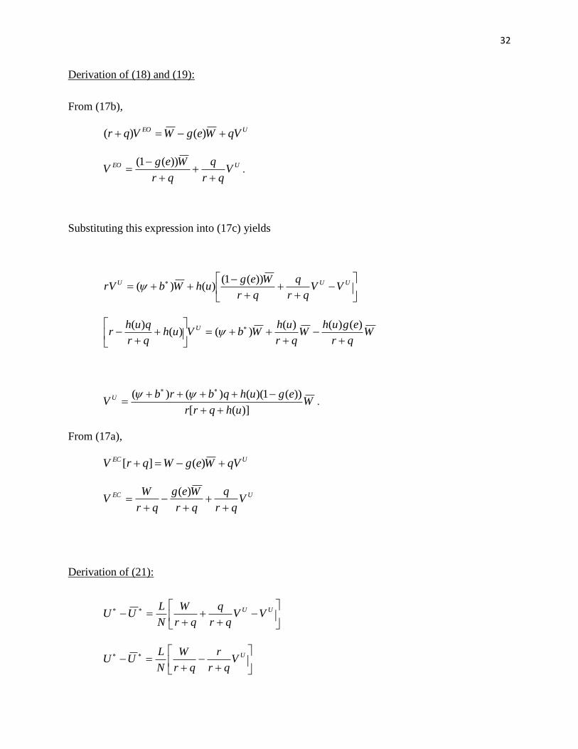
Derivation of (18) and (19):
From (17b),
UEO qVWegWVqr )()(
UEO Vqr
q
qr
WegV
))(1(.
Substituting this expression into (17c) yields
UUU VV
qr
q
qr
WeguhWbrV
))(1()()(
Wqr
eguhW
qr
uhWbVuh
qr
quhr U
)()()(
)()()(
Wuhqrr
eguhqbrbV U
)]([
))(1)(()()(
.
From (17a),
UEC qVWegWqrV )(][
UEC V
qr
q
qr
Weg
qr
WV
)(
Derivation of (21):
UU VV
qr
q
qr
W
N
LUU
UV
qr
r
qr
W
N
LUU

33
W
uhqrqr
uhbqbr
qr
tW
N
LUU
)]()[(
)()(
Wuhqrqr
uhbqbr
qr
WrPuhWWe
YADWcqr
WN
UUa
)]()[(
)()()](,/[
)1(
11
)1)(1(1)1(
)1(1
11
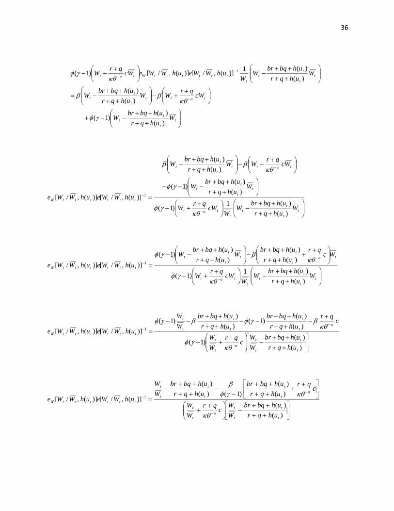
Derivation of (22):
dW
dUU
dW
UUd
))(1(
)(0
)1(
1)1(
)1(
1)1(
1
1
)1)(1(1)1(
)](,/[)1(
1)](,/[)](,/[)1(
)1(
)1)(1(1
)1(
1)(
uhWWeWcqr
W
Wcqr
WW
uhWWeuhWWe
SDrPYA
dW
d
a
aW
qruhWWeWc
qrW
Wuhqrqr
uhbqbr
qr
W
WuWWeuhWWeWc
qrW
Wuhqrqr
uhbqbr
qr
WuhWWeWc
qrW
N
rPYAD
dW
UUd
a
Wa
a
tt
1)](,/[
)]()[(
)(
1],/[)](,/[)1(
)]()[(
)()](,/[)1(
)()1(
1
)(
)1(
1
1)1(
1
)1(
2
)1)(1(1)1(1
1

34
)1(
1)1(
)1(
1)1(
1
1
)1)(1(1)1(
)1(
1
1)1(
1
)1(
2
)1)(1(1)1(1
1
)](,/[)1(
1)](,/[)](,/[)1(
)1(
)1)(1(1
)1(
1)())(1(
1)](,/[
)]()[(
)(
1],/[)](,/[)1(
)]()[(
)()](,/[)1(
)()1(
1
0
ttttat
tat
t
tttWttt
ttttt
ttttat
t
t
tt
t
tttWttttat
t
t
tt
ttttat
ttt
t
uhWWeWcqr
W
Wcqr
WW
uhWWeuhWWe
BDrPAYUU
qruhWWeWc
qrW
Wuhqrqr
uhbqbr
qr
W
WuWWeuhWWeWc
qrW
Wuhqrqr
uhbqbr
qr
WuhWWeWc
qrW
N
rPAYD
)](,/[)1(1
)](,/[)1(
)1(
)1)(1(1))(1(
1)](,/[
)]()[(
)(1)](,/[)1(
)]()[(
)()](,/[)1(
10
1)1()1(
1
1
2
ttttattat
t
tttW
tt
ttttat
t
t
tt
t
tttWtat
t
t
tt
ttttatt
uhWWeWcqr
WWcqr
WW
uhWWe
BUU
qruhWWeWc
qrW
Wuhqrqr
uhbqbr
qr
W
WuhWWeWc
qrW
Wuhqrqr
uhbqbr
qr
WuhWWeWc
qrW
N

35
)](,/[)1(1
)](,/[)1(
)1(
)1)(1(1
)]()[(
)()(
)](,/[)1(
11)1(
1)](,/[
)]()[(
)(1)](,/[)1(
)]()[(
)()](,/[)1(
1
)1(
)1)(1(1
)1(
1)()](,/[0
1)1()1(
)1)(1(
1)1()1(1
11
1
1
2
)1(
1
1
)1)(1(1)1()1(
ttttattat
t
tttW
t
t
tt
ttttttat
ttttat
t
t
tt
t
tttWtat
t
t
tt
ttttat
at
tt
e
tttt
uhWWeWcqr
WWcqr
WW
uhWWe
BW
uhqrqr
uhbqbr
qr
Wr
PuhWWeAYDWcqr
WN
qruhWWeWc
qrW
Wuhqrqr
uhbqbr
qr
W
WuhWWeWc
qrW
Wuhqrqr
uhbqbr
qr
WuhWWeWc
qrW
N
BWc
qrW
DrPuhWWeAY
)](,/[)1(1
)](,/[)1()(
)()1(
)](,/[)(
)(1)](,/[)1(
)(
)()](,/[)1(0
ttttat
t
tttWt
t
t
t
ttttatt
t
t
t
t
tttWtat
t
t
t
tttt
uhWWeWcqr
WW
uhWWeWuhqr
uhbqbrW
uhWWeWcqr
WWuhqr
uhbqbrW
WuhWWeWc
qrW
Wuhqr
uhbqbrWuhWWe
t
t
t
t
tatt
t
t
t
tat
t
ttttttWt
t
t
t
t
t
t
t
t
ttttttWtat
Wuhqr
uhbqbrW
Wcqr
WWuhqr
uhbqbrW
Wcqr
WW
uhWWeuhWWeWuhqr
uhbqbrW
Wuhqr
uhbqbrW
WuWWeuhWWeWc
qrW
)(
)()1()1(
)(
)()1(
1)](,/[)](,/[)1(
)(
)()1(
)(
)(1],/[)](,/[)1(
1
1
36
t
t
t
t
tatt
t
t
t
t
t
t
t
t
ttttttWtat
Wuhqr
uhbqbrW
Wcqr
WWuhqr
uhbqbrW
Wuhqr
uhbqbrW
WuhWWeuhWWeWc
qrW
)(
)()1(
)(
)(
)(
)(1)](,/[)](,/[)1( 1
t
t
t
t
t
tat
t
t
t
t
tatt
t
t
t
ttttttW
Wuhqr
uhbqbrW
WWc
qrW
Wuhqr
uhbqbrW
Wcqr
WWuhqr
uhbqbrW
uhWWeuhWWe
)(
)(1)1(
)(
)()1(
)(
)(
)](,/[)](,/[ 1
t
t
t
t
t
tat
tat
t
t
t
t
t
ttttttW
Wuhqr
uhbqbrW
WWc
qrW
Wcqr
uhqr
uhbqbrW
uhqr
uhbqbrW
uhWWeuhWWe
)(
)(1)1(
)(
)(
)(
)()1(
)](,/[)](,/[ 1
)(
)()1(
)(
)()1(
)(
)()1(
)](,/[)](,/[ 1
t
t
t
t
a
t
t
at
t
t
t
t
t
ttttttW
uhqr
uhbqbr
W
Wc
qr
W
W
cqr
uhqr
uhbqbr
uhqr
uhbqbr
W
W
uhWWeuhWWe
)(
)(
)(
)(
)1()(
)(
)](,/[)](,/[ 1
t
t
t
t
a
t
t
a
t
t
t
t
t
t
ttttttW
uhqr
uhbqbr
W
Wc
qr
W
W
cqr
uhqr
uhbqbr
uhqr
uhbqbr
W
W
uhWWeuhWWe

37
Derivation of (25):
)(
)(11
)(
)(
)1()(
)(1
)](,1[)](,1[ 1
uhqr
uhbqbrc
qr
cqr
uhqr
uhbqbr
uhqr
uhbqbr
uheuhe
a
a
W
)(
))(1(1
)(
)(
)1()(
))(1(
)](,1[)](,1[ 1
uhqr
qrbc
qr
cqr
uhqr
uhbqbr
uhqr
qrb
uheuhe
a
a
W
))(1(1
)]()[()()(
)1())(1(
)](,1[)](,1[ 1
qrbcqr
cuhqrqr
uhqrbqrb
uheuhe
a
a
W
cqr
cuhqr
qr
uhb
buheuhe
a
a
W
1
)()(
)1)(1(1
)](,1[)](,1[ 1
a
a
a
a
a
a
W
u
uqcqr
u
uqc
u
uqqr
qr
u
uq
bb
u
uqe
u
uqe
11
1
11
1
1
)1()(1
)1()1(
)1(
)1)(1(1
)1(,1
)1(,1

38
Derivations of du/d, du /db, du /dc, du /d, and du /dq:
a
a
a
a
a
aW
u
uqc
u
uqqr
uqr
uqb
b
u
uqcqr
u
uqe
u
uqe
11
1
11
1
1
)1()1(
)(
)1(
)1)(1(1
)1()(1]
)1(,1[]
)1(,1[
(A4)
Let 0)1()1(
)(
)1( 11
1
a
a
a
u
uqc
u
uqqr
uqr
uqbZ
Totally differentiating (A4) with respect to u, , b, q, c, and yields:
2
1
12
1
1
2
11
1
11
11
1
2
11
1
222
2
1
12
11
2
11
11
1
1
1
2
21
1
1
2
11
1
1
)1()1()1(
1)1)(1(
)1()1(
)1)(1(
)1(
)1)(1(
)1()1(
)1)(1(1
1
)1()1(
)1)(1(
)(
)()1(
)1)(1()1)(1()1)(1()1)(1(
)1()1(
1
)1()(
1
)1()(
)1(],1[],1[
)1(],1[],1[],1[
)1()(1
)1(],1[],1[
)1()(1
u
udquqdu
u
uqc
u
uqqr
a
a
b
u
udquqdu
u
uqc
b
dqu
uqc
bd
u
uqc
u
uqqr
ba
dcu
uq
u
uqqr
b
uqr
duqrqdquru
bb
db
b
dbZ
b
Zd
u
udquqdu
u
uq
a
ad
u
uqcqr
a
a
dcu
uqqrdq
u
uqchehe
u
udquqduhehehe
u
uqcqr
u
udquqduhehe
u
uqcqr
a
a
a
a
a
a
a
a
aa
a
a
a
a
a
a
a
a
a
a
a
a
a
a
aa
a
aW
hW
a
a
a
Wh
a
a
a

39
dqu
u
u
uqc
u
uqqr
a
a
b
u
u
u
uqc
bu
uqc
b
uqr
ur
bu
uhehehe
u
uqcqr
u
uhehe
u
uqcqr
u
u
u
uqcqr
a
ahehe
u
uqchehe
du
uqc
u
uqqr
baqr
a
ahehe
dcu
uq
u
uqqr
bqrhehe
dbb
bZd
b
Z
duu
uqc
u
uqqr
a
a
b
u
uqc
bqrb
u
uq
a
acqrhehehehehe
u
uqcqr
heheu
uqcqr
u
q
a
a
a
a
a
aa
a
a
hW
a
a
a
Wh
a
a
a
a
a
aW
a
a
aW
a
a
a
a
W
a
a
aW
a
a
a
a
a
a
a
a
aWhW
a
a
a
Wh
a
a
a
)1()1()1(
1)1)(1(
)1()1(
)1)(1(
)1(
)1)(1(
)(
)1(
)1)(1(
)1(],1[],1[],1[
)1()(1
)1(],1[],1[
)1()(1
)1()1()(
1],1[],1[
)1(],1[],1[
)1()1(
)1)(1(1
1)(
1],1[],1[
)1()1(
)1)(1()(],1[],1[
)1)(1(
)1(
)1)(1(
)1()1(
1)1)(1(
)1(
)1)(1(
1
)1)(1(
)1(
1)(],1[],1[],1[],1[],1[
)1()(1
],1[],1[)1(
)(1
1
12
1
1
11
11
1
1
2
21
1
1
11
1
1
1
12
1
1
11
1
1
1
11
2
1
11
1
1
2
1
12
1
1
11
1
1
12
1
1
121
1
1
11
1
1
2
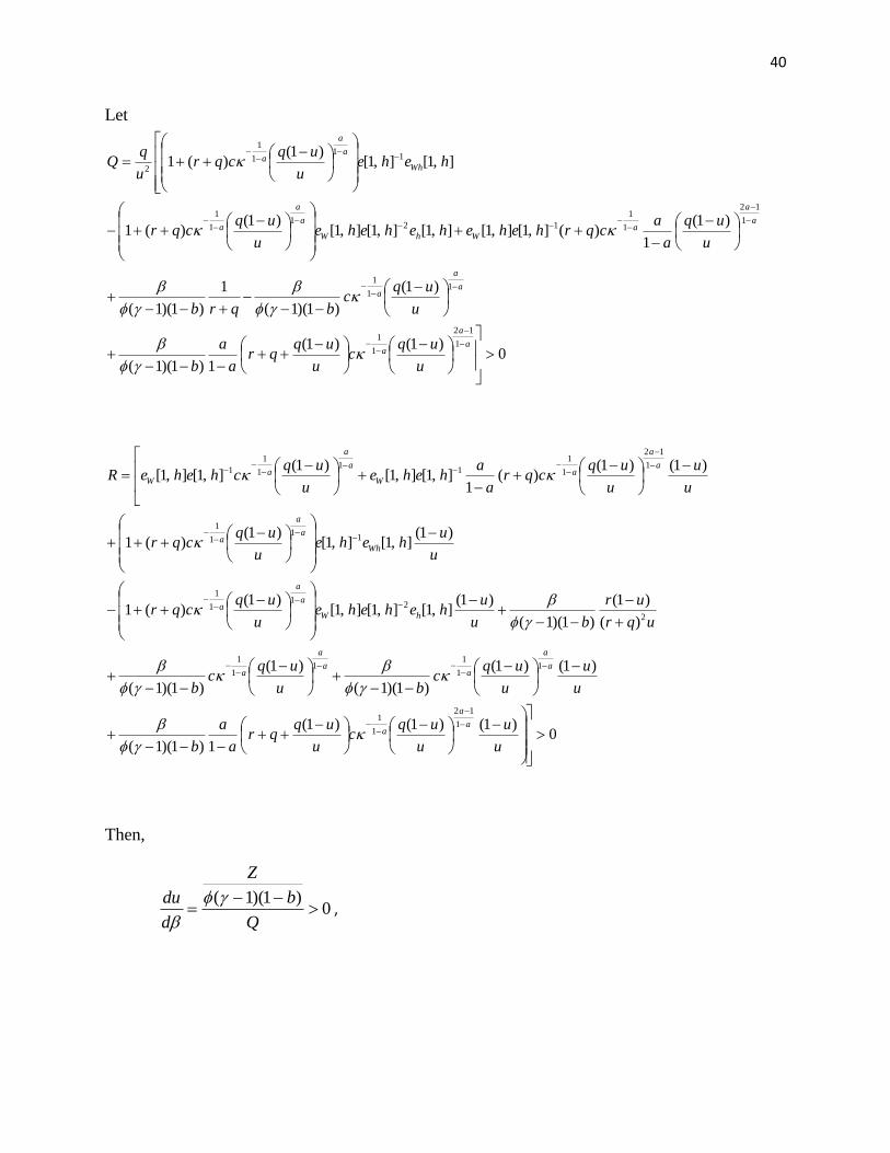
40
Let
0)1()1(
1)1)(1(
)1(
)1)(1(
1
)1)(1(
)1(
1)(],1[],1[],1[],1[],1[
)1()(1
],1[],1[)1(
)(1
1
12
1
1
11
1
1
12
1
1
121
1
1
11
1
1
2
a
a
a
a
a
a
a
a
aWhW
a
a
a
Wh
a
a
a
u
uqc
u
uqqr
a
a
b
u
uqc
bqrb
u
uq
a
acqrhehehehehe
u
uqcqr
heheu
uqcqr
u
0)1()1()1(
1)1)(1(
)1()1(
)1)(1(
)1(
)1)(1(
)(
)1(
)1)(1(
)1(],1[],1[],1[
)1()(1
)1(],1[],1[
)1()(1
)1()1()(
1],1[],1[
)1(],1[],1[
1
12
1
1
11
11
1
1
2
21
1
1
11
1
1
1
12
1
1
11
1
1
1
u
u
u
uqc
u
uqqr
a
a
b
u
u
u
uqc
bu
uqc
b
uqr
ur
bu
uhehehe
u
uqcqr
u
uhehe
u
uqcqr
u
u
u
uqcqr
a
ahehe
u
uqcheheR
a
a
a
a
a
aa
a
a
hW
a
a
a
Wh
a
a
a
a
a
aW
a
a
aW
Then,
0)1)(1(
Q
b
Z
d
du
,

41
,0)1)(1(
)1(2
Q
b
bZ
db
du
,0
)1()1(
)1)(1()(],1[],1[
11
1
1
Q
u
uq
u
uqqr
bqrhehe
dc
du
a
a
aW
,0
)1(
)1)(1(
)1(
1
1)(
1],1[],1[
11
2
1
Q
u
uqc
b
u
uqqr
aqr
a
ahehe
d
du
a
a
a
a
W

42
0Q
R
dq
du.
Derivation of du/dz:
With the shift variable, z, for changes in We , (A4) can be expressed as
a
a
a
a
a
aW
u
uqc
u
uqqr
uqr
uqb
b
u
uqcqrz
u
uqez
u
uqe
11
1
11
1
1
)1()1(
)(
)1(
)1)(1(1
)1()(1],
)1(,1[],
)1(,1[
with 0Wze , 0ze .
Totally differentiating the above equation with respect to u and z yields
QdudzzhezheWz 1],,1[],,1[
0],,1[],,1[ 1
Q
zhezhe
dz
du Wz
Derivation of (30)
)(
)(
)(
)(
)1(],/[],/[ 1
thqr
thbqbr
W
Wc
qr
W
W
cqr
thqr
thbqbr
hqr
hbqbr
W
W
hWWehWWe
t
t
a
t
t
at
t
t
t
ttttttW

43
1
1111
1
1
111
1
1
1
1
1
1
1
1
)1(
]1[])1([)(
])1([)()1(
]1[
)1()1(
]1[
,)1(
,
tt
tt
t
ta
a
ta
a
ttta
t
t
a
a
ta
a
ttta
tt
tt
tt
tt
t
t
t
t
t
t
ttt
t
t
W
uruq
uquqbqbr
W
Wcuuuuqqr
W
W
cuuuuqqruruq
uquqbqbr
uruq
uquqbqbr
W
W
uW
We
u
uuuq
W
We
1
1
1
1
111
1
1
111
1
1
1
1
1
111
1
1
1
1
)1(
]1[])1([)(
])1([)()1(
]1[
)1(
])1([)(
,)1(
,
tt
tt
t
ta
a
ta
a
ttta
t
t
a
a
ta
a
ttta
tt
tt
a
a
ta
a
ttta
t
t
t
t
t
t
ttt
t
tW
uruq
uquqbqbr
W
Wcuuuuqqr
W
W
cuuuuqqruruq
uquqbqbr
cuuuuqqrW
W
uW
We
u
uuuq
W
We
1
1
1
111
1
1
1
1
111
1
11
1
)1(
]1[
])1([)()1(
]1[
)1(1
])1([)(,)1(
,
tt
tt
t
t
a
a
ta
a
ttta
tt
tt
a
a
ta
a
ttta
t
tt
t
t
t
ttt
t
tW
uruq
uquqbqbr
W
W
cuuuuqqruruq
uquqbqbr
cuuuuqqrW
Wu
W
We
u
uuuq
W
We

44
1
)1(
]1[])1([)(
)1(
]1[
)1(
])1([)(,)1(
,
1
1
1111
1
1
1
1
111
1
11
1
tt
tt
t
ta
a
ta
a
ttta
tt
tt
a
a
ta
a
ttta
t
tt
t
t
t
ttt
t
tW
uruq
uquqbqbr
W
Wcuuuuqqr
uruq
uquqbqbr
cuuuuqqrW
Wu
W
We
u
uuuq
W
We

45
0
)1(
]1[
])1([)(1
])1([)(1
)1(])1([)(1
])1([
))(1(
])1([
))()(1(
)1(
])1([
))(1(
])1([
))()(1(1
)1(
]1[
])1([)()1(
]1[
)1(
],/[],/[
])1([)(1
])1([)(1
)1(])1([)(1
1
])1([)(
)(],/[],/[],/[)/(],/[],/[
)/1(],/[],/[)(
],/[],/[
)/(],/[],/[)/1(],/[],/[
1
1
1
111
12
11
1
1
1
11
1
1
11
12
11
1
12
1
2
1
1
12
1
2
1
1
2
2
1
1
111
1
1
1
1
1
11
12
11
1
1
1
11
1
1
11
12
11
1
2
111
1
1
2
12222
22
2
11
211
tt
tt
t
t
ta
a
ta
a
tta
ta
ta
a
tta
ta
a
ta
a
tta
t
tt
tt
tt
t
t
tt
tt
tt
tt
t
tt
t
tt
tt
t
t
a
a
ta
a
ttta
tt
tt
ttttttW
ta
a
tta
ta
ta
a
tta
ta
a
ta
a
tta
t
t
tt
t
a
a
ta
a
tta
t
t
ttttthttttttWtttttttttW
ttttttttWtt
ttttttWh
tttttttttWWttttttttWW
uruq
uquqbqbr
W
W
duuuuqqcqra
a
duuuuqqcqra
aduquuuqqcqr
a
a
duuruq
urqbdu
uruq
uqrqb
duuruq
urqbdu
uruq
uqrqbWd
W
WdW
W
uruq
uquqbqbr
W
W
uuuuqcqruruq
uquqbqbr
hWWehWWe
duuuqqcqra
aduuuuqqcqr
a
a
duuquuqqcqra
aWd
W
WdW
W
uuuqqcqrW
W
u
duquuduhWWehWWehWWeWdWWhWWehWWe
dWWhWWehWWeu
duquuduhWWehWWe
WdWWhWWehWWedWWhWWehWWe

46
Let
a
a
a
a
aW uuqcqrhehes 111
1
1
1 )]1([)(1],1[],1[
1
111
1
1
))(1()]1([)(
][
)1(1
ruq
qrbcuuqqr
ruq
quqbqbrs a
a
ta
a
a
a
a
a
a
a uuqcqrruq
quqbqbr
ruq
quqbqbr
s
111
12
)]1([)(][
][
a
a
a
a
a
a
a
a
a
a
uuqcqrruq
quqbqbr
uuqcqrs
111
1
111
1
2
)]1([)(][
)]1([)(1
a
a
a
a
a uuqcqr
s
111
13
)]1([)(1
1
a
a
a
a
a
a
a
a
a
a
uuqcqr
uuqcqrs
111
1
111
1
3
)]1([)(1
)]1([)1
1][
1
14
ruq
quqbqbrs
0][
1
][
1 4
ruq
quqbqbr
ruq
quqbqbr
s
47
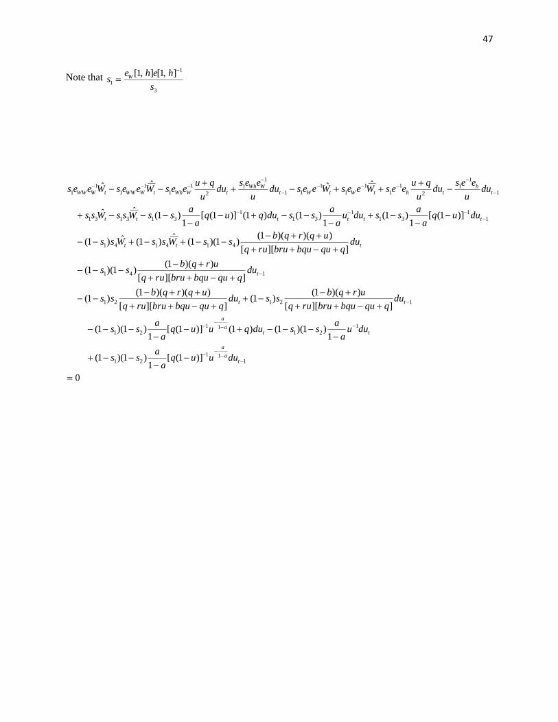
Note that 3
1
1
],1[],1[
s
hehes W
0
)]1([1
)1)(1(
1)1)(1()1()]1([
1)1)(1(
]][[
))(1()1(
]][[
))()(1()1(
]][[
))(1()1)(1(
]][[
))()(1()1)(1(
ˆ)1(ˆ)1(
)]1([1
)1(1
)1()1()]1([1
)1(ˆˆ
ˆˆˆˆ
111
21
1
2111
21
12121
141
414141
1
1
31
1
31
1
313131
1
1
1
2
1
1
1
1
1
11
1
1
2
1
1
1
1
1
1
ta
a
tta
a
tt
t
ttt
tttttt
th
thtWtWtWWh
tWWhtWWWtWWW
duuuqa
ass
duua
assduquuq
a
ass
duqqubqubruruq
urqbssdu
qqubqubruruq
uqrqbss
duqqubqubruruq
urqbss
duqqubqubruruq
uqrqbssWssWss
duuqa
assduu
a
assduquq
a
assWssWss
duu
eesdu
u
queesWeesWeesdu
u
eesdu
u
queesWeesWees
48
111
2121
41
1
31
1
1
1
1
1
2111
21
2141
1
31
1
312
1
12
1
14131
1
1
1
1
4131
1
1
1
1
)]1([1
)1)(1(]][[
))(1()1(
]][[
))(1()1)(1()]1([
1)1(
1)1)(1()1()]1([
1)1)(1(
]][[
))()(1()1(
]][[
))()(1()1)(1(
1)1(
)1()]1([1
)1(ˆ
)1(
ˆ)1(
ta
a
hWWh
ta
a
t
hWWhtWWWW
tWWWW
duuuqa
ass
qqubqubruruq
urqbss
qqubqubruruq
urqbssuq
a
ass
u
ees
u
ees
duua
assquuq
a
ass
qqubqubruruq
uqrqbss
qqubqubruruq
uqrqbssu
a
ass
quqa
ass
u
quees
u
queesWsssseesees
Wsssseesees
111
2121
41
1
31
1
1
1
1
1
2111
21
2141
1
31
1
312
1
12
1
141
1
1
1
1
41
1
1
1
1
)]1([1
)1)(1(]][[
))(1()1(
]][[
))(1()1)(1()]1([
1)1(
1)1)(1()1()]1([
1)1)(1(
]][[
))()(1()1(
]][[
))()(1()1)(1(
1)1(
)1()]1([1
)1(ˆ
)1()1(
ˆ)1()1(
ta
a
hWWh
ta
a
t
hWWhtWWWW
tWWWW
duuuqa
ass
qqubqubruruq
urqbss
qqubqubruruq
urqbssuq
a
ass
u
ees
u
ees
duua
assquuq
a
ass
qqubqubruruq
uqrqbss
qqubqubruruq
uqrqbssu
a
ass
quqa
ass
u
quees
u
queesWsseesees
Wsseesees
(A5)
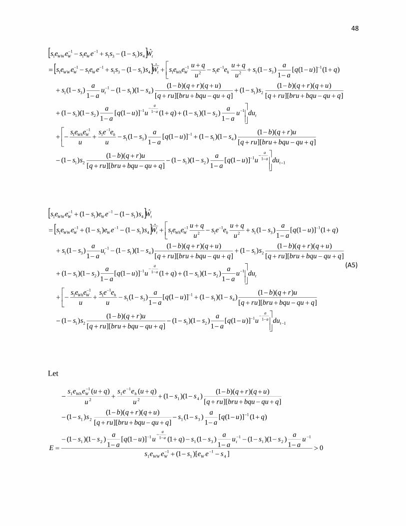
Let
0])[1(
1)1)(1(
1)1()1()]1([
1)1)(1(
)1()]1([1
)1(]][[
))()(1()1(
]][[
))()(1()1)(1(
)()(
4
1
1
1
1
1
21
1
3111
21
1
3121
412
1
1
2
1
1
seesees
ua
assu
a
assquuq
a
ass
quqa
ass
qqubqubruruq
uqrqbss
qqubqubruruq
uqrqbss
u
quees
u
quees
EWWWW
ta
a
hWWh

49
and
0])[1(
)]1([1
)1)(1()]1([1
)1(]][[
))(1()1(
]][[
))(1()1)(1(
4
1
1
1
1
11
21
1
3121
41
1
1
1
1
seesees
uuqa
assuq
a
ass
qqubqubruruq
urqbss
qqubqubruruq
urqbss
u
ees
u
ees
FWWWW
a
a
hWWh
The first four terms of E are greater than the first four terms of F by the factor (q +u)/u, and the
fifth and sixth terms in E are greater than the fifth term in F by the factor (1+q), thus implying that
E>F. Given these expressions for E and F, (A5) be expressed as
1
ˆˆ tttt FduEduWW . (A6)
Assume each period, a fraction, , of firms can adjust their wages. Then, following the derivation
in Romer (2012) and Campbell (2017), wage inflation can be expressed as
1
,
11
)]1(1[
1
)]1(1[
tt
ew
t
w
t FduEdu
. (A7)
From (9),
])[1( 123121
,
1
,
1
w
TtT
w
t
w
t
w
t
uew
t
ew
t . (A8)
Substituting (A8) into (A7) yields

50
1
123121
,
1
1
)]1(1[
1
)]1(1[])[1(
t
t
w
TtT
w
t
w
t
w
t
uew
t
w
t
Fdu
Edu
1
12312
,
11
1
)]1(1[
1
)]1(1[])[1(])1(1[
t
t
w
TtT
w
t
w
t
uew
t
w
t
Fdu
Edu
1
1
11
1
1
1
,
1
])1(1)[1(
)]1(1[
])1(1)[1(
)]1(1[
)1(1
)1(
)1(1
t
t
T
j
w
jtjuew
tw
t
Fdu
Edu
(A9)
Equation (A9) can be expressed as
143
1
12
,
11
tt
T
j
w
jtj
uew
t
w
t dudu
where 0)1(1 1
1
,
0)1(1
)1(
1
2
,
0])1(1)[1(
)]1(1[
1
3
E
,
0])1(1)[1(
)]1(1[
1
4
F
.
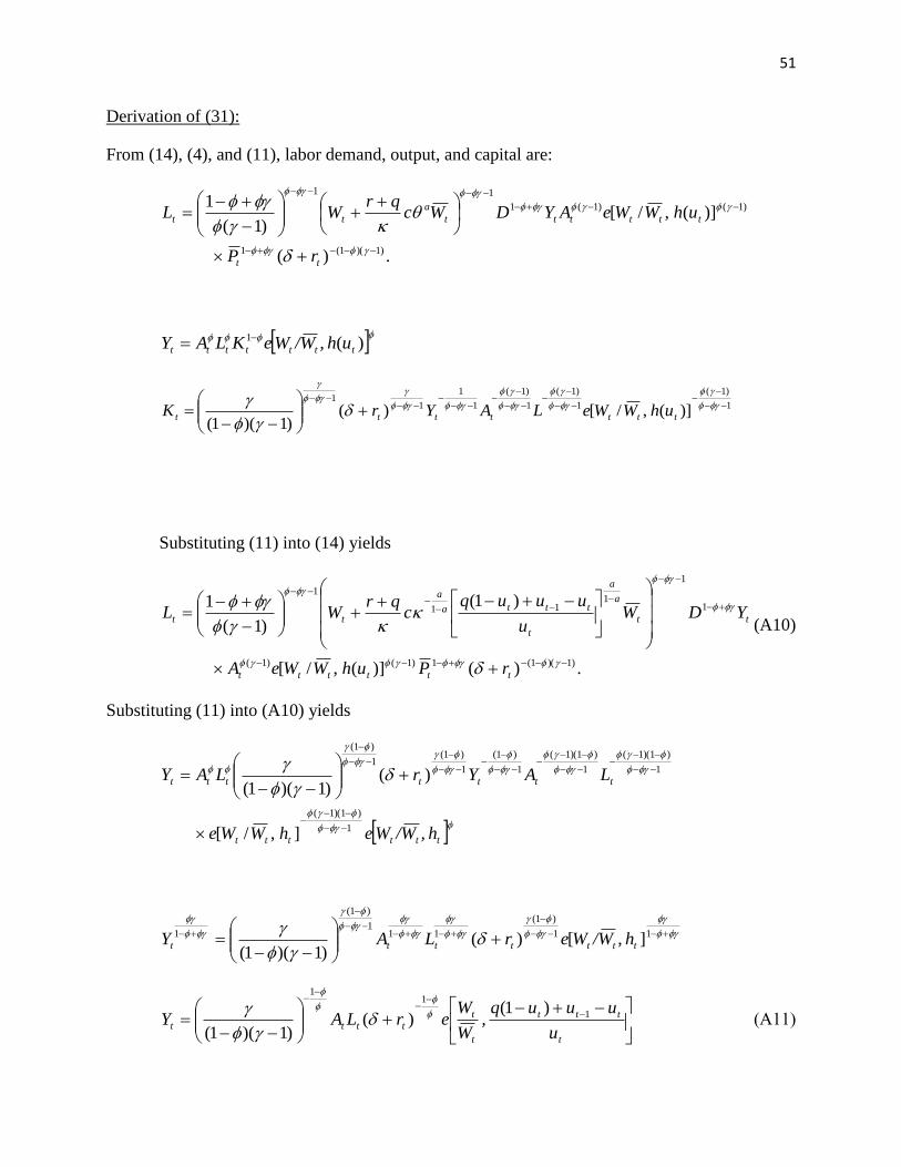
51
Derivation of (31):
From (14), (4), and (11), labor demand, output, and capital are:
.)(
)](,/[)1(
1
)1)(1(1
)1()1(1
11
tt
tttttt
a
tt
rP
uhWWeAYDWcqr
WL
)(1
ttttttt uh,W/WeKLAY
1
)1(
1
)1(
1
)1(
1
1
11
)](,/[)()1)(1(
ttttttt uhWWeLAYrK
Substituting (11) into (14) yields
.)()](,/[
)1(
)1(
1
)1)(1(1)1()1(
1
1
111
1
tttttt
tt
a
a
t
ttta
a
tt
rPuhWWeA
YDWu
uuuqc
qrWL
(A10)
Substituting (11) into (A10) yields
tttttt
ttttttt
h,W/WehWWe
LAYrLAY
1
)1)(1(
1
)1)(1(
1
)1)(1(
1
)1(
1
)1(1
)1(
],/[
)()1)(1(
11
)1(
111
)1(
1 ][)()1)(1(
ttttttt h,W/WerLAY
t
ttt
t
t
ttttu
uuuq,
W
WerLAY 1
11
)1()(
)1)(1(
(A11)

52
Totally differentiating (A11) and dividing by the original equation yields the following expression,
in terms of deviations from steady-state values:
1
1
2
1
11 )(ˆˆ1ˆˆˆ
th
th
tWtWtrttt duu
eedu
u
uqeeWeeWeedrsLAY
(A12)
where
r
sr
1 .
Totally differentiating (8a) and dividing by the original equation yields
)1(ˆˆ
1
t
ttt
r
drYY
.
Letting e
t represent expected price inflation, the IS curve can be expressed as
)(ˆˆ1
e
ttrtt ddisYY , where )]1(/[1 rsr . (A13)
Similarly, totally differentiating (8b) and dividing by the original expressions gives
ttt
t
t
t
tttt
ttt diii
YP
i
i
i
diidii
YPM)1(
1ˆˆ
1
)1(
)1(
1ˆˆˆ2
,
which can be approximated by
tittt disYPM ˆˆˆ , where )]1(/[1 iisi . (A14)
An equation for the price level can be obtained by substituting tdi in (A13) into (A14), yielding
)ˆˆ(ˆˆˆ1
e
trtt
r
ittt dsYY
s
sYMP ,
which can be expressed as

53
e
titttt dsYYMP 1ˆˆ)1(ˆˆ
, where 0r
i
s
s .
e
tit
th
th
tWtWtrtttt
dsY
duu
eedu
u
uqeeWeeWeedrsLAMP
1
1
1
2
111
ˆ
)(ˆˆ1ˆˆ)1(ˆˆ
e
titth
th
tWtWtrtttt
dsYduu
eedu
u
uqee
WeeWeedrsLAMP
11
1
2
1
11
ˆ)1()(
)1(
ˆ)1(ˆ)1(1
)1(ˆ)1(ˆ)1(ˆˆ
(A15)
Totally differentiating (A10) and dividing by the original equation yields
trtth
th
tWtWtt
tW
tW
tWtWt
drsPduu
ee
duu
uqeeWeeWeeAY
duu
aas
duu
uqaasWsWsL
)1)(1(ˆ)1()1(
)()1(ˆ)1(ˆ)1(ˆ)1(ˆ
)]1/()[1)(1(
))](1/()[1)(1(ˆ)1)(1(ˆ)1(ˆ
1
1
2
111
1
2
(A16)
where a
W
cqr
s
1
1.
Substituting (A12) and (A15) into (A16) yields

54
e
titth
th
tWtW
trttttr
th
th
tWtW
t
th
th
tWtWtrtt
tW
tW
tWtWt
dsYduu
eedu
u
uqee
WeeWee
drsLAMdrs
duu
eedu
u
uqeeWeeWee
A
duu
eedu
u
uqeeWeeWeedrsLA
duu
aas
duu
uqaasWsWsL
11
1
2
1
11
1
1
2
111
1
1
2
111
1
2
ˆ)1()(
)1(
ˆ)1(ˆ)1(
1)1(ˆ)1(ˆ)1(ˆ)1()1)(1(
)1()()1(ˆ)1(ˆ)1(
ˆ)1(
)(ˆˆ1ˆˆ
)]1/()[1)(1(
))](1/()[1)(1(ˆ)1)(1(ˆ)1(ˆ
The unemployment rate can be expressed as
N
LNu t
t
.
Differentiating this expression yields
tLt
t LsN
dLdu ˆ
,
where N
LsL .
Thus, tL̂ can be expressed as
tLt dusL 1ˆ .

55
e
titth
th
tr
tLtttr
th
th
tth
th
trt
tW
tW
t
dsYduu
ee
duu
uqeedrs
dusAMdrs
duu
eedu
u
uqee
Aduu
eedu
u
uqeedrsA
duu
aas
duu
uqaasW
)1(ˆ)1()1)(1(
)()1)(1(
1)1)(1(
)1()1(ˆ)1)(1(ˆ)1()1)(1(
)1()()1(
ˆ)1()(1ˆ
)]1/()[1)(1(
))](1/()[1)(1(ˆ)1(0
11
1
2
1
1
1
1
2
1
1
1
2
1
1
2
trrr
e
tittt
th
Wh
th
L
hWt
drsss
dsYAM
duu
ee
u
aas
u
ee
duu
uqees
u
uqee
u
uqaasW
)1)(1(11
)1)(1(
)1(ˆ)1(ˆ)1(ˆ)1(
)1(
)]1/()[1)(1()1)(1(
)(1)1()1(
)()1())](1/()[1)(1(ˆ)1(
1
1
1
1
2
1
1
2
1
2
trr
e
tittttWh
tLh
LhW
t
drss
dsYAMduu
aas
u
ee
duu
uqsees
u
uqee
u
uqaasW
)1()()1(
1
ˆˆˆ)]1/()[1(
)(1)1(
)())](1/()[1(ˆ
11
1
2
1
1
2
1
2
(A17)

56
Subtracting the lag of (A17) from (A17) results in the following expression for wage inflation
)ˆˆ( 1 tt
w
t WW :
)()1(
)()ˆˆ(
)ˆˆ()ˆˆ()()]1/()[1(
)()(
1)1()())](1/()[1(
111
1121
1
12
1
1
2
1
2
ttre
t
e
titt
ttttttWh
ttLh
LhWw
t
drdrs
ddsYY
AAMMduduu
aas
u
ee
duduu
uqsees
u
uqee
u
uqaas

57
References
Basu, Susanto, John G. Fernald, and Miles S. Kimball, (2006). “Are Technology Improvements
Contractionary?” American Economic Review, Vol 96(5), December 2006, pp. 1418-1448.
Basu, Susanto, John G. Fernald, Jonas Fisher, and Miles S. Kimball, (2013). “Sector-Specific
Technical Change,” Manuscript, 2013.
Calvo, Guillermo (1983). “Staggered Prices in a Utility-Maximizing Framework,” Journal of
Monetary Economics, vol. 12, September 1983, pp. 383-398.
Campbell, C.M. (2006). “A model of the determinants of effort,” Economic Modelling, vol. 23(2),
pp. 215-37.
Campbell, Carl M. (2014). “The formation of wage expectations in the effort and quit decisions of
workers,” Economic Modelling. Vol. 42, pp. 313-22.
Campbell, Carl M. (2017). “Efficiency Wage Setting, Labor Demand, and Phillips Curve
Microfoundations,” Working Paper, Northern Illinois University. (An earlier version of the
paper is available at Munich Personal RePEc Archive (MPRA) Working Paper #74984,
October 2016, https://mpra.ub.uni-muenchen.de/74984/1/MPRA_paper_74984.pdf).
Campbell, Carl M., and John V. Duca (2008). “The Impact of Evolving Labor Practices and
Demographics on U.S. Inflation and Unemployment,” Paper presented at Markets and
Models: Policy Frontiers in the AWH Phillips Tradition, 49th Annual Conference of the
New Zealand Association of Economists, Wellington, New Zealand, July 2008.
http://nzae.org.nz/wp-content/uploads/2011/08/nr1215387056.pdf.
Dixit, A.K. and Stiglitz, J.E. (1977). “Monopolistic competition and optimum product diversity,”
American Economic Review, vol. 67(3), pp. 297-308.
Fuhrer, J.C. (1997). ‘The (un)importance of forward-looking behavior in price specifications,’
Journal of Money, Credit, and Banking, vol. 29(3), pp. 338-50.
Galí, J. (2011). “The return of the wage Phillips curve,” Journal of the European Economic
Association, vol. 9(3), pp. 436-61.
Layard, Richard, Stephen Nickell, and Richard Jackman (1991). Unemployment: Macroeconomic
Performance and the Labour Market. Oxford: Oxford University Press.
Levine, P., Pearlman, J., Perendia, G. and Yang, B. (2012). “Endogenous persistence in an
estimated DSGE model under imperfect information,” Economic Journal, vol. 122(565),
pp. 1287-1312.
58
Lindé, Jesper, (2005). “Estimating New-Keynesian Phillips Curves: A Full Information Maximum
Likelihood Approach,” Journal of Monetary Economics, vol. 52, pp. 1135-1149.
Perry, G.L. (1978). “Slowing the wage-price spiral: the macroeconomic view,” Brookings Papers
on Economic Activity, vol. 1978:2, pp. 259-99.
Pfajfar, D. and Santoro, E. (2010). ‘Heterogeneity, learning and information stickiness in inflation
expectations,’ Journal of Economic Behavior and Organization, vol. 75(3), pp. 426-44.
Phelps, E.S. (1968). “Money-wage dynamics and labor-market equilibrium,” Journal of Political
Economy, vol. 76(4), pp. 678-711.
Pissarides, Christopher A. (2000). Equilibrium Unemployment Theory, 2nd edition. Cambridge,
MA: MIT Press.
Roberts, J.M. (1997). ‘Is inflation sticky?’ Journal of Monetary Economics, vol. 39(2), pp. 173-
96.
Romer, David. (2012). Advanced Macroeconomics, New York: McGraw-Hill.
Salop, S.C. (1979). “A model of the natural rate of unemployment,” American Economic Review,
vol. 69(1), pp. 117-25.
Schlicht, E. (1978). “Labour Turnover, Wage Structure and Natural Unemployment,” Zeitschrift
für die Gesamte Staatswissewnschaft, vol. 134(2), pp. 337-46.
Shapiro, C. and Stiglitz, J.E. (1984). “Equilibrium unemployment as a worker discipline device,”
American Economic Review, vol. 74(3), pp. 433-44.
Shimer, Robert, (2005). “The Cyclical Behavior of Equilibrium Unemployment and Vacancies,”
American Economic Review, vol. 95(1), pp. 25-49.
Shimer, Robert, (2007). “Reassessing the Ins and Outs of Unemployment,” NBER Working Paper
No. 13421, September 2007.
Stiglitz, J.E. (1974). “Alternative theories of wage determination and unemployment in L.D.C.’s:
The labor turnover model,” Quarterly Journal of Economics, vol. 88(2), pp. 194-227.

59
Table 1
Estimates of the Phillips Curve and Dynamic Labor Demand Curve
1967:2-2017:1 1967:2-2007:4
1 2 3 4
Phillips curve w/ e w/ e
tu -0.2371a
(-3.01)
-0.2497a
(-2.86)
-0.3017b
(-2.25)
-0.3069c
(-1.70)
1tu 0.1959b
(2.26)
0.2126b
(2.18)
0.2342c
(1.69)
0.2347
(1.23) w
t 1 0.325a
(3.04)
0.304b
(2.36)
0.403a
(3.49)
0.417a
(2.81)
w
t 1 0.199a
(2.93)
0.203a
(2.80)
0.201a
(2.97)
0.194c
(1.96)
w
t 2 - w
t 4 0.323a
(11.77)
0.353a
(12.51)
0.279a
(9.20)
0.275a
(7.85)
w
t 5 - w
t 8 0.038
(0.13)
0.028
(0.07)
0.162
(2.35)
0.152
(2.10)
w
t 9 - w
t 12 0.138
(2.44)
0.134
(2.15)
-0.012
(-.01)
0.002
(0.00)
12
11 j
w
jt
w
t 1.024
1.021 1.032 1.040
1 tt uu -0.0411a
(8.00)
-0.0371b
(5.53)
-0.0675a
(9.90)
-0.0722a
(7.88)

60
t-statistic reported in parentheses for single coefficients; Likelihood Ratio statistic reported
for sums of coefficients
a significant at the 1% level b significant at the 5% level c significant at the 10% level
Table 1 (continued)
1967:2-2017:1 1967:2-2007:4
DLD 1 2 3 4
tu 3.25a
(2.92)
2.91a
(2.89)
1.86a
(3.17)
1.66a
(3.02)
1tu -3.73a
(-2.72)
-3.19a
(-2.63)
-2.05a
(-2.89)
-1.84b
(-2.52)
2tu 0.475
(1.19)
0.298
(0.85)
0.140
(0.51)
0.141
(0.47)
A -0.545a
(12.26)
-0.651a
(17.11)
-0.183c
(3.09)
-0.265a
(7.02)
OilPrice 0.0217a
(13.00)
0.0158a
(7.22)
0.0194a
(17.60)
0.0195a
(16.89)
M 0.528a
(16.80)
0.657a
(26.37)
0.618a
(27.38)
0.705b
(36.05)
Vtrend 0.150a
(4.00)
0.161a
(5.02)
0.173a
(3.64)
0.186a
(4.26)
Y 1.380a
(41.45)
1.478a
(42.56)
0.416a
(7.48)
0.498a
(11.87)
r 0.551a
(12.47)
0.411a
(9.54)
0.584a
(23.93)
0.478a
(20.09) e
0.844a
(8.21)
0.378c
(3.54)
21 ttt uuu -0.0038 0.0238 -0.056 -0.035
M+ Vtrend 0.678 0.818 0.791 0.891
LR test:
021 ttt uuu
0.01 0.50 2.95c 0.98
LR test: A=–Y 17.26a 17.58a 2.53 2.65
LR test:
M+ Vtrend=
2.57 0.15 0.30 0.36
61
Footnotes
1 At the margin, workers supply labor up to the point where the marginal utility of leisure equals the wage. For a
worker who is involuntarily unemployed, the marginal utility of leisure is less than the wage. All things being equal,
as the average wage rises, the marginal utility of leisure for those who are unemployed will be higher. In addition,
unemployment benefits generally rise as average wages increase. 2 While many quits are into another job rather than into unemployment, it is likely that the probability of finding
another job when employed is closely related to the probability of finding a job when unemployed. Thus, the
probability of hire for an unemployed worker should be related to both quits into unemployment and quits into a
different job. 3 The Cobb-Douglas is a commonly used functional form for the matching function. See, for example, Romer
(2012). 4 It is assumed that the coefficient of relative risk aversion is the same in both the utility of consumption and in
the utility of real money holdings. 5 See Pissarides (2000), pp. 68-70 for an exposition of the search and matching model for large firms. 6 See Figure 7 of Campbell and Duca (2008) for the simulation of the natural rate and see Figure 6 for the
simulation of the duration-unemployment ratio. This paper is available at http://nzae.org.nz/wp-
content/uploads/2011/08/nr1215387056.pdf. 7 See equation 25 on p. 698 of Phelps (1968).
8 In (31), the DLD in levels is .)1(ˆˆˆˆ 1
1121 tr
e
titttttt drsdsYAMduduW
9 Another potential instrument from (31) is expected price inflation, but its inclusion reduces the sample size. 10 Government defense spending was also considered for an instrument, but it had a very low significance level
and often had a negative sign. 11 The 3-month Treasury Bill rate is used in the regressions since both (8a) and (8b) suggest a short-term interest
rate is the appropriate variable. 12 Because the current and recent lagged values of trend velocity are highly correlated with one another, the sum
of the current and three lagged changes in trend velocity is entered as a single variable.