A Microeconomic Approach to

Diffusion Models for Stock Prices*

Hans Follmer

Institut fur Angewandte Mathematik

Universitat Bonn

Wegelerstraße 6

D-W-5300 Bonn 1

Germany

Martin Schweizer

Institut fur Mathematische Stochastik

Universitat Gottingen

Lotzestraße 13

D-W-3400 Gottingen

Germany

(Mathematical Finance 3 (1993), 1–23)

* This is a slightly modified version; it already incorporates the Erratum published in

Mathematical Finance 4 (1994), 285.

Abstract:

This paper studies a class of diffusion models for stock prices derived by a microeco-nomic approach. We consider discrete-time processes resulting from a market equilibriumand then apply an invariance principle to obtain a continuous-time model. The resultingprocess is an Ornstein-Uhlenbeck process in a random environment, and we analyze itsqualitative behavior. In particular, we provide simple criteria for the stability or instabil-ity of the corresponding stock price model, and we give explicit formulae for the invariantdistributions in the recurrent case.

Key words:

stock price models, invariance principle, Ornstein-Uhlenbeck process, random environment,invariant distribution, noise traders, information traders

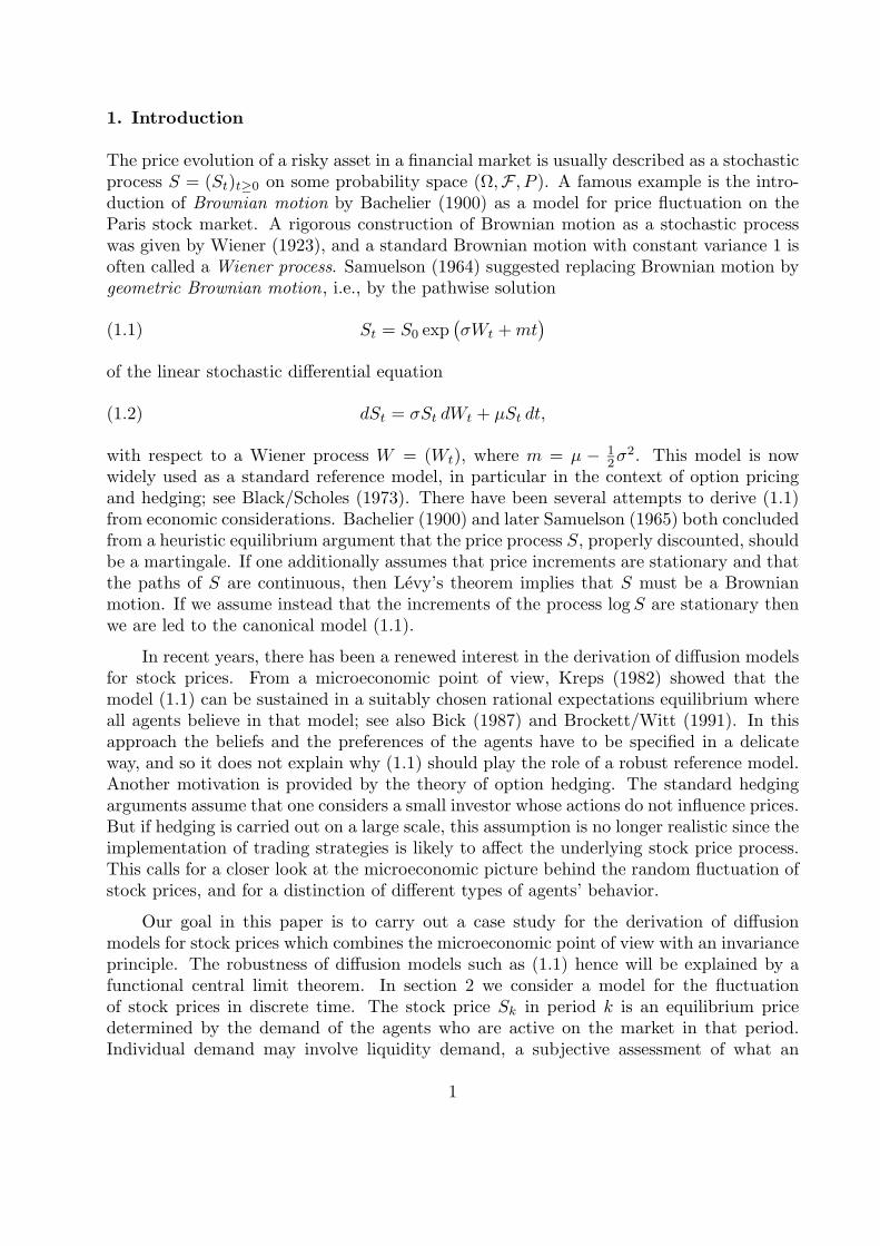
1. Introduction

The price evolution of a risky asset in a financial market is usually described as a stochasticprocess S = (St)t≥0 on some probability space (Ω,F , P ). A famous example is the intro-duction of Brownian motion by Bachelier (1900) as a model for price fluctuation on theParis stock market. A rigorous construction of Brownian motion as a stochastic processwas given by Wiener (1923), and a standard Brownian motion with constant variance 1 isoften called a Wiener process. Samuelson (1964) suggested replacing Brownian motion bygeometric Brownian motion, i.e., by the pathwise solution

(1.1) St = S0 exp(σWt +mt

)

of the linear stochastic differential equation

(1.2) dSt = σSt dWt + µSt dt,

with respect to a Wiener process W = (Wt), where m = µ − 12σ

2. This model is nowwidely used as a standard reference model, in particular in the context of option pricingand hedging; see Black/Scholes (1973). There have been several attempts to derive (1.1)from economic considerations. Bachelier (1900) and later Samuelson (1965) both concludedfrom a heuristic equilibrium argument that the price process S, properly discounted, shouldbe a martingale. If one additionally assumes that price increments are stationary and thatthe paths of S are continuous, then Levy’s theorem implies that S must be a Brownianmotion. If we assume instead that the increments of the process logS are stationary thenwe are led to the canonical model (1.1).

In recent years, there has been a renewed interest in the derivation of diffusion modelsfor stock prices. From a microeconomic point of view, Kreps (1982) showed that themodel (1.1) can be sustained in a suitably chosen rational expectations equilibrium whereall agents believe in that model; see also Bick (1987) and Brockett/Witt (1991). In thisapproach the beliefs and the preferences of the agents have to be specified in a delicateway, and so it does not explain why (1.1) should play the role of a robust reference model.Another motivation is provided by the theory of option hedging. The standard hedgingarguments assume that one considers a small investor whose actions do not influence prices.But if hedging is carried out on a large scale, this assumption is no longer realistic since theimplementation of trading strategies is likely to affect the underlying stock price process.This calls for a closer look at the microeconomic picture behind the random fluctuation ofstock prices, and for a distinction of different types of agents’ behavior.

Our goal in this paper is to carry out a case study for the derivation of diffusionmodels for stock prices which combines the microeconomic point of view with an invarianceprinciple. The robustness of diffusion models such as (1.1) hence will be explained by afunctional central limit theorem. In section 2 we consider a model for the fluctuationof stock prices in discrete time. The stock price Sk in period k is an equilibrium pricedetermined by the demand of the agents who are active on the market in that period.Individual demand may involve liquidity demand, a subjective assessment of what an

1

adequate price should be, as well as a technical demand arising from dynamic strategies ofportfolio insurance. In this paper we shall model these relations in the setting of a simplelog-linear structure of individual excess demand.

If liquidity demand is the only source of randomness in our model, and if this random-ness has a classical i.i.d. structure, then logarithmic stock prices Xk = logSk perform arandom walk with a drift. By the invariance principle, this random walk converges undersuitable rescaling to a Brownian motion

(1.3) Xt = σWt +mt

with volatility σ and drift parameter m. This means that stock prices themselves willconverge to a geometric Brownian motion (1.1); see, e.g., Duffie/Protter (1992). But ifexcess demand involves other components then we should expect a different equilibriumprice structure and, via an invariance principle, a different limiting diffusion model. Fol-lowing Black (1986), we consider in particular a class of information traders and a classof noise traders. In our model the excess demand of information traders depends in alog-linear way on their perceptions of an underlying fundamental level, while noise traderstake the proposed equilibrium price as a signal for that level. In a log-linear simplifica-tion, the demand of technical traders is analogous to the demand of noise traders. Theprocess of logarithmic stock prices, centered around a sequence of aggregates of perceivedfundamental levels, then takes the form

(1.4) Xk −Xk−1 = βkXk−1 + εk.

Here we have two sources of randomness. The quantities (εk) are averages of individualliquidity demand. The behavioral quantities (βk) aggregate the individual agents’ ways ofreacting to a proposed equilibrium price based on their perceptions of what an adequateprice should be. In this second source, randomness may for instance appear as a fluctuationin the proportion between different types of agents. Information traders contribute negativevalues to βk. If only information traders are active on the market, the logarithmic priceprocess therefore performs a recurrent fluctuation of Ornstein-Uhlenbeck type around theaggregate fundamental levels. But if the effect of noise trading and of technical tradingbecomes too dominant then βk may assume positive values. In such periods the Ornstein-Uhlenbeck process changes from its usual recurrent to a highly transient behavior. Witha different interpretation, a model of the form (1.4) is also considered by Orlean/Robin(1991) who discuss its stability, using a criterion of Brandt (1986).

To make the qualitative behavior of the process (1.4) more transparent and explicit,we apply in section 3 an invariance principle to its two sources of randomness to pass to adiffusion model in continuous time. This leads to a stochastic differential equation of theform

(1.5) dXt = Xt(σtdWt + mtdt) + σtdWt +mtdt

where W and W are Wiener processes with covariance process d〈W ,W 〉t = %tdt. In thesimple special case

(1.6) dXt = mXtdt+ σdWt,

2

the price process is a geometric Ornstein-Uhlenbeck process. For m < 0, this process isergodic with a log-normal invariant distribution and provides a natural reference modelin the class of stationary price processes. The solution of the general case (1.5) maybe viewed as an Ornstein-Uhlenbeck process in a random environment. In section 4 weinvestigate its qualitative behavior under the assumption that et = (σt, mt, σt,mt, %t) isan ergodic process. Extending a result of Brandt (1986) from discrete time to the settingof (1.5), we derive a bound for the aggregate effect of noise trading which assures thatthe induced price fluctuation remains a stationary ergodic process. Beyond that boundthe price process becomes highly transient. In fact we shall show that the paths convergeeither to 0 or to ∞, and that their growth or decay exceeds an exponential rate.

In section 5 we consider the special case where the process e is a deterministic con-stant. The random environment of the Ornstein-Uhlenbeck process is then described bythe Wiener process W . For m < 1

2 σ2 the price fluctuation is ergodic, and we can give

explicit formulae for the density of the invariant distribution. But the situation is morevolatile than in the classical case (1.6). Typically, the invariant distribution is a mixtureof normal distributions, and the mixing measure on the variances has unbounded sup-port. In particular we obtain fatter tails than in the classical model (1.1), and S does nothave moments of any order. Explicit examples also show that a continuous but singulardistribution may appear as the mixing measure.

The present paper works out some ideas which were stated in an informal manner inFollmer (1991). Thanks are due to Alan Kirman whose suggestion to consider models witha random fluctuation between different groups of agents provided the initial motivation forthis work; see also Kirman (1993).

2. The micro-economic model

Let us describe a simple model for the evolution of the price of a speculative asset. Weconsider a finite set A of agents who are active on the market. Given a proposed stockprice p, each agent a ∈ A forms an excess demand ea(p). The equilibrium stock price S isthen determined by the market clearing condition of zero total excess demand. Since wethink of a temporal sequence of markets at discrete times tk (k = 0, 1, ...), we add a timesubscript k to A, ea and S. We also add a parameter ω which summarizes all variablesother than p which may influence agents’ decisions. We view ω as a sample point in someunderlying probability space (Ω,F , P ), and so the temporal sequence of equilibrium pricesbecomes a stochastic process

(2.1) Sk(ω) (k = 0, 1, ...)

defined by the implicit equations

(2.2)∑

a∈Ak(ω)

ea,k(Sk(ω), ω

)= 0.

3

In order to derive explicit results with a minimum of technicalities, we assume thatthe individual excess demand in period k is of the log-linear form

(2.3) ea,k(p, ω) = αa,k(ω) logSa,k(ω)

p+ δa,k(ω),

typically with αa,k ≥ 0. Here δa,k may be viewed as a liquidity demand, and Sa,k denotes an

individual reference level of agent a for period k. For instance, Sa,k could be interpreted asa price expectation for the following period, but we will also consider other interpretationsin the examples below. Clearly, the particular form (2.3) is too simple to be a realisticmodel of excess demand and can only be viewed as a first approximation to a more generaldemand behavior. In particular, we have not imposed any explicit budget constraintand we leave aside interest rates. The log-linear excess demand function is often used inmonetary models; see for instance Cagan (1956), Gourieroux/Laffont/Monfort (1982) orLaidler (1985).

The explicit form (2.3) of individual excess demand permits us to solve (2.2) for theequilibrium stock price to obtain

(2.4) logSk(ω) =∑

a∈Ak(ω)

αa,k(ω) log Sa,k(ω) + δk(ω)

with

(2.5) αa,k = (∑

a∈Akαa,k)−1αa,k, δk = (

∑

a∈Akαa,k)−1

∑

a∈Akδa,k.

Thus, the actual logarithmic equilibrium stock price is a weighted average of individuallogarithmic price assessments and of liquidity demands.

(2.6) Remark. In a model of a rational expectations equilibrium, one would assume thatall agents have beliefs consistent with the underlying probability measure P . Specifically,let us suppose that the individual price assessments are given by

(2.7) Sa,k = E [Sk+1|Ftk ] ,

where Ftk is the σ-algebra of events observable to all agents up to time tk. In the absenceof liquidity demand, (2.4) and (2.7) would imply

(2.8) Sk = E [Sk+1|Ftk ]

so that stock prices form a martingale; see Tirole (1982). Note that there is no discountinghere since our excess demand itself does not contain a discount factor. In contrast to thisapproach, we do not assume in our subsequent discussion that the objective probabilitymeasure P on Ω is known to the agents.

4

Consider the simple special case Sa,k = Sk−1 so that

(2.9) logSk(ω) = logSk−1(ω) + δk(ω).

Under standard i.i.d. assumptions on the sequence (δk) of aggregate liquidity demands, thelogarithmic price process X = logS becomes a random walk. Under a passage from discreteto continuous time with suitable rescaling, the process X would converge to a Brownianmotion with drift. Thus, the resulting price process S = exp(X) would be a geometricBrownian motion as in (1.1). But as soon as the individual assessments Sa,k depend in amore complex manner on past experience, on individual perceptions of fundamental valuesor of the proposed price taken as a signal, we must expect that other diffusion modelswill appear in the limit. In the following examples we try to capture, in a very simplifiedmanner, different types of agents’ behavior by introducing different specifications of theindividual reference level Sa,k.

(2.10) Examples. 1) For an information trader, or fundamentalist, the individual ref-erence level is determined by his current perception Fa,k(ω) of the fundamental value ofthe asset and by his belief how the actual stock price will be attracted to that value.Specifically, let us assume that an information trader chooses a reference level of the form

(2.11) log Sa,k = logSk−1 + βa,k(logSk−1 − logFa,k)

with a random coefficient βa,k(ω) ≤ 0. If only such information traders were active on themarket, the resulting price process would be of the form

(2.12) logSk = logSk−1 + βk(logSk−1 − logFk) + δk

with

(2.13) βk =∑

a∈Akαa,kβa,k, logFk =

1

βk

∑

a∈Akαa,kβa,k logFa,k.

As will be explained more carefully below, this suggests that the logarithmic price processinduced by information traders behaves like an Ornstein-Uhlenbeck process around a time-dependent level. It will be an Ornstein-Uhlenbeck process in a random environment sinceboth the levels and the coefficients (βk) are random processes.2) In a simplified model of noise trading, we assume that the reference level of a noisetrader is of the form

(2.14) logSa,k = logSk−1 + γa,k(logSk−1 − log p)

with some random coefficient γa,k(ω) ≤ 0. Thus, the proposed price is taken seriously as asignal and replaces the fundamental quantity Fa,k in (2.11). Suppose that only such noisetraders are active on the market. Then we have

(2.15) logSk = logSk−1 + γk(logSk−1 − logSk) + δk,

5

hence

(2.16) logSk = logSk−1 + εk,

where

(2.17) εk = (1 + γk)−1δk, γk =∑

a∈Akαa,kγa,k.

This suggests that the logarithmic price process should have the structure of a randomwalk. We will see below that the effect of noise trading becomes more drastic if noisetraders interact with information traders.3) In a simplistic log-linear approximation, the technical excess demand arising from dy-namical strategies of portfolio insurance (see for instance Black/Jones (1987)) would takethe form

(2.18) αa,k(logSk−1 − log p)

with a random coefficient αa,k(ω) ≤ 0. Taken together with the agent’s liquidity demand,

the resulting excess demand is of the form (2.3) with Sa,k = Sk−1, but now with a coefficientof negative sign. If only such traders are active on the market, it follows as in 2) that theresulting logarithmic price process will have the structure of a random walk. Here again,the effect of such traders will become more drastic if they start to interact with informationtraders.

Let us now study the interactive effect of the different types of behavior described inthe preceding examples. To this end we assume that the individual reference level is of theform

(2.19) logSa,k = logSk−1 + βa,k(logSk−1 − logFa,k) + γa,k(logSk−1 − log p)

with random coefficients βa,k(ω) ≤ 0 and γa,k(ω) ≤ 0. As in (2.12) and (2.16), the resultingprice process takes the form

(2.20) logSk = logSk−1 + βk(logSk−1 − logFk) + εk

where

(2.21) γk =∑

a∈Akαa,kγa,k, βk = (1 + γk)−1

∑

a∈Akαa,kβa,k, εk = (1 + γk)−1δk,

and where Fk is a logarithmic mixture of the individual assessments Fa,k. Note that therandom coefficients βk may become positive if the effect of either the noise traders (largeabsolute values of γk) or the portfolio insurers (negative values of αa,k) becomes too strong.

Equation (2.20) will be the basis for our subsequent analysis. Note that it containsthree, in general correlated, sources of randomness: the behavioral quantities (βk), the

6

aggregate liquidity demand (εk), and the uncertainty about the fundamentals containedin the aggregate quantities (Fk). If we define the level Lk recursively by

Lk = (1 + βk)Lk−1 − βk logFk, L0 = logF0,

then the process

Xk = logSk − Lk (k = 0, 1, ...)

satisfies

(2.22) Xk −Xk−1 = βkXk−1 + εk.

Thus, the logarithmic price process may be viewed as an Ornstein-Uhlenbeck process ina random environment which fluctuates around the time-dependent process (Lk). Moreprecisely, the process (Xk) is an Ornstein-Uhlenbeck process centered around 0 where boththe additive quantities (εk) and the multiplicative quantities (βk) are random processes.Recall that βk may become positive if either noise trading or portfolio insurance becomestoo dominant. In such periods, the Ornstein-Uhlenbeck process will change from its usualrecurrent behavior to a highly unstable transient behavior. These features will be analyzedin more detail for the diffusion approximation obtained in the next section.

In this paper, we are not interested in that part of the randomness which is inducedby fluctuations in the fundamentals. In fact, experiments clearly show that one shouldexpect a random fluctuation of asset prices even if the uncertainty about the fundamentalsis completely eliminated; cf., e.g., Smith/Suchanek/Williams (1988). In the context of ourmodel, we will concentrate on the effect of the two sources (εk) and (βk) of randomness.Therefore we may as well assume that the sequence (Fk), and hence the sequence (Lk), isequal to some deterministic constant. Thus, our price process is of the form

(2.23) Sk = exp(Xk + L) (k = 0, 1, ...)

where the process (Xk) is given by equation (2.22).

(2.24) Remark. Price processes of the type (2.22) have previously appeared in the lit-erature; see for instance Froot/Obstfeld (1991), Shiller (1981), Summers (1986) or West(1988). In our present approach, we motivate these processes from a microeconomic pointof view, in terms of assumptions at the level of individual agents. This will allow us tostudy the effect that different types of behavior and a random fluctuation of the pro-portion between different groups of agents have on the resulting equilibrium stock priceprocess. Similar models have been suggested or studied by Black (1986), Day/Huang(1989), De Long/Shleifer/Summers/Waldmann (1990a,b), Follmer (1974), Frankel/Froot(1986), Goodhart (1988), Grossman (1988), Hart/Kreps (1986) and Kirman (1993), amongothers.

7

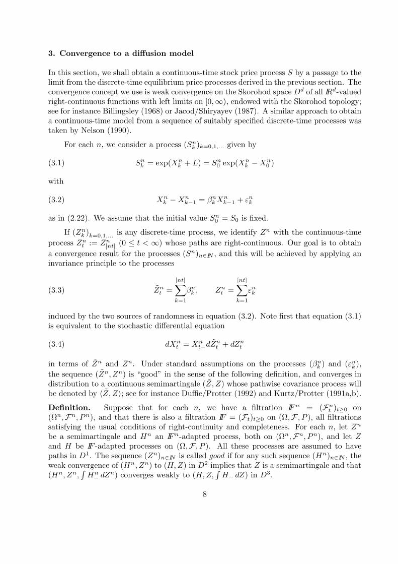
3. Convergence to a diffusion model

In this section, we shall obtain a continuous-time stock price process S by a passage to thelimit from the discrete-time equilibrium price processes derived in the previous section. Theconvergence concept we use is weak convergence on the Skorohod space Dd of all IRd-valuedright-continuous functions with left limits on [0,∞), endowed with the Skorohod topology;see for instance Billingsley (1968) or Jacod/Shiryayev (1987). A similar approach to obtaina continuous-time model from a sequence of suitably specified discrete-time processes wastaken by Nelson (1990).

For each n, we consider a process (Snk )k=0,1,... given by

(3.1) Snk = exp(Xnk + L) = Sn0 exp(Xn

k −Xn0 )

with

(3.2) Xnk −Xn

k−1 = βnkXnk−1 + εnk

as in (2.22). We assume that the initial value Sn0 = S0 is fixed.

If (Znk )k=0,1,... is any discrete-time process, we identify Zn with the continuous-time

process Znt := Zn[nt] (0 ≤ t < ∞) whose paths are right-continuous. Our goal is to obtain

a convergence result for the processes (Sn)n∈IN , and this will be achieved by applying aninvariance principle to the processes

(3.3) Znt =

[nt]∑

k=1

βnk , Znt =

[nt]∑

k=1

εnk

induced by the two sources of randomness in equation (3.2). Note first that equation (3.1)is equivalent to the stochastic differential equation

(3.4) dXnt = Xn

t−dZnt + dZnt

in terms of Zn and Zn. Under standard assumptions on the processes (βnk ) and (εnk ),

the sequence (Zn, Zn) is “good” in the sense of the following definition, and converges indistribution to a continuous semimartingale (Z, Z) whose pathwise covariance process willbe denoted by 〈Z, Z〉; see for instance Duffie/Protter (1992) and Kurtz/Protter (1991a,b).

Definition. Suppose that for each n, we have a filtration IFn = (Fnt )t≥0 on(Ωn,Fn, Pn), and that there is also a filtration IF = (Ft)t≥0 on (Ω,F , P ), all filtrationssatisfying the usual conditions of right-continuity and completeness. For each n, let Zn

be a semimartingale and Hn an IFn-adapted process, both on (Ωn,Fn, Pn), and let Zand H be IF -adapted processes on (Ω,F , P ). All these processes are assumed to havepaths in D1. The sequence (Zn)n∈IN is called good if for any such sequence (Hn)n∈IN , theweak convergence of (Hn, Zn) to (H,Z) in D2 implies that Z is a semimartingale and that(Hn, Zn,

∫Hn− dZ

n) converges weakly to (H,Z,∫H− dZ) in D3.

8

(3.5) Theorem. Suppose that (Zn, Zn) is good and converges in distribution to the con-tinuous semimartingale (Z, Z). Then (Zn, Zn, Xn) converges in distribution to (Z, Z,X)where X is the strong solution

(3.6) Xt = exp(Zt −1

2〈Z〉t)(X0 +

∫ t

0

exp(− (Zs −

1

2〈Z〉s)

)d(Z − 〈Z, Z〉)s)

of the stochastic differential equation

(3.7) dXt = XtdZt + dZt.

Moreover, the price processes Sn (n = 1,2,...) converge in distribution to the process

(3.8) St = exp(Xt + L).

Proof. The weak convergence of (Zn, Zn, Xn) in D3 to (Z, Z,X) follows from the resultsof SÃlominski (1989); see also Kurtz/Protter (1991a,b). Ito’s formula implies that (3.6)solves (3.7); cf. Protter (1990), Theorem V.52. Finally, the weak convergence of Sn to Sfollows by the continuous mapping theorem.

(3.9) Examples. 1) Suppose that the first source of randomness in equation (3.2) canbe neglected as we pass to the continuous-time limit, i.e., assume that Z = 0. Then (3.6)reduces to

(3.10) Xt = X0 + Zt.

Under homogeneity assumptions on the second source of randomness, Z will be a Brownianmotion with constant variance and constant drift:

(3.11) dZt = σdWt +mdt.

In that case, the price process S is given by the usual reference model

(3.12) St = S0 exp(σWt +mt)

of geometric Brownian motion.2) Suppose that, in the limit, the first source of randomness in equation (3.2) produces anabsolutely continuous drift, but no additional noise. In other words, assume that

(3.13) Zt =

∫ t

0

msds (t ≥ 0).

If Z is given by (3.11) with m = 0, the limiting equation (3.7) reduces to

(3.14) dXt = mtXtdt+ σdWt.

9

In the special homogeneous case where mt(·) = m , we obtain

(3.15) dXt = mXtdt+ σdWt,

i.e., X is an Ornstein-Uhlenbeck process, transient for m > 0 and recurrent for m < 0. Inthis model, the logarithmic price process logS performs an Ornstein-Uhlenbeck fluctuationaround the level L, and the price process S will be called a geometric Ornstein-Uhlenbeckprocess. In the recurrent case m < 0, this process may be viewed as a canonical referencemodel in the class of stationary price processes. In the general case (3.14) where thecoefficient fluctuates randomly, the process X is an Ornstein-Uhlenbeck process in a randomenvironment.

In the next section we consider a general class of such processes in a random environ-ment and study their qualitative behavior in situations where the environment is ergodic.

4. Ornstein-Uhlenbeck processes in an ergodic random medium

In this section we want to analyze the behavior of the limiting stock price process Scorresponding to equation (3.7) in a situation where the two sources of randomness forma stationary ergodic environment. More precisely, we assume that (Z, Z) is of the form

(4.1) dZt = mtdt+ σtdWt, dZt = mtdt+ σtdWt

with

(4.2) d〈Z, Z〉t = σtσtd〈W ,W 〉t = γtdt,

where W ,W are standard Brownian motions with random correlation (%t) so that γt =σtσt%t. We assume that the process

(4.3) et = (mt, σt,mt, σt, γt) is ergodic,

and that (et) and the white noise processes corresponding to W ,W are defined for alltimes t ∈ IR on some probability space (Ω,F , P ). We also introduce the integrabilityassumptions

(4.4) mt, σ2t ,mt, σ

2t , γt ∈ L1(Ω,F , P ).

Let us first prove some general facts concerning the pathwise asymptotic behavior ofthe stock price process S = (St).

(4.5) Theorem. If

(4.6) c = E[m0 −1

2σ2

0 ] > 0,

10

then the stock price S exhibits superexponential growth or decay, i.e.,

(4.7) limt↑∞

1

tlog | logSt| = c P − a.s.

Proof. 1) The continuous martingale

(4.8) Mt =

∫ t

0

σsdWs (t ≥ 0)

satisfies

(4.9) limt↑∞

Mt

t= 0 P − a.s.

This is clear if E[σ20 ] = 0. If E[σ2

0 ] > 0 then the quadratic variation

(4.10) 〈M〉t =

∫ t

0

σ2sds (t ≥ 0)

of M satisfies

(4.11) limt↑∞

1

t〈M〉t = E[σ2

0 ] > 0 P − a.s.

by the ergodic theorem. In particular we have 〈M〉∞ =∞, hence

(4.12) limt↑∞

Mt

〈M〉t= 0 P − a.s.

by the law of large numbers for continuous martingales. But (4.12) together with (4.11)implies (4.9).

2) By the ergodic theorem, the process

(4.13) Ct =

∫ t

0

(ms −1

2σ2s)ds

satisfies

(4.14) limt↑∞

1

tCt = c P − a.s.

We have

(4.15) Xt = (X0 +Mt + Ct) exp(Mt + Ct)

11

with

(4.16) Mt =

∫ t

0

e−(Ms+Cs)σsdWs

and

(4.17) Ct =

∫ t

0

e−(Ms+Cs)(ms − γs)ds.

Due to (4.9) and (4.14), it is enough to show that both M and C converge P -a.s. to afinite limit. Again by (4.9) and (4.14), the total variation |C| of C satisfies

(4.18) |C|t ≤ |C|t(ε) +

∫ ∞

0

e−(c−ε)s|ms − γs|ds

for 0 < ε < c, and the second term has finite expectation due to assumption (4.4). Thisimplies the convergence of C to some finite limit, P -a.s. Similarly, the local martingale Mhas quadratic variation

(4.19) 〈M〉t ≤ 〈M〉t(ε) +

∫ ∞

0

e−2(c−ε)sσ2sds,

where the second term has finite expectation. Thus M converges P -a.s. to some finitelimit.

Theorem (4.5) says that for c > 0, stock prices are not stable in any sense: Thetrajectories either tend to 0 or go off to infinity. Note that this is quite different from thebehavior of geometric Brownian motion (3.12) where

(4.20) limt↑∞

1

tlogSt = µ− 1

2σ2 P − a.s.

According to the sign of µ− 12σ

2, the geometric Brownian motion either goes to 0 P -a.s. orto +∞ P -a.s., in both cases at an exponential rate. In contrast, growth and decay inTheorem (4.5) can both occur with positive probability, and the situation is much moreinstable since the convergence rate is higher than exponential.

We have seen in the previous section that a recurrent geometric Ornstein-Uhlenbeckprocess may be viewed as a canonical stationary model for price fluctuations. Let usnow show in our general situation that we get recurrent behavior if the environment ison average not too destabilizing, i.e., if c < 0. The following result is a continuous-timeversion of a theorem of Brandt (1986) for discrete-time processes of the form (2.22).

In addition to (4.4), we need some further integrability assumptions in order to guar-antee that

(4.21) log+(

∫ 1

0

e−(Zs− 12 〈Z〉s)d(Z − 〈Z, Z〉)s) ∈ L1.

12

By standard estimates on the moments of stochastic integrals, condition (4.21) follows if,

e.g., m0, σ20 , γ0 ∈ L2 and E[epσ

20 ] <∞ for p = 16.

(4.22) Theorem. If

(4.23) c = E[m0 −1

2σ2

0 ] < 0,

the logarithmic price process X converges to an ergodic process:

(4.24) limt↑∞|Xt − X0 θt| = 0 P − a.s.

where

(4.25) X0 =

∫ 0

−∞exp

(−∫ 0

s

d(Z − 1

2〈Z〉)u

)d(Z − 〈Z, Z〉)s

is P-a.s. well-defined. In particular, the distribution of Xt converges to the distribution ofX0.

Proof. 1) The formal definition (4.25) of X0 should be read as

(4.26) X0 = limn→−∞

eV0−Vn∫ 0

n

e−(Vs−Vn)dVs,

where

(4.27) dVs = dZs − d〈Z, Z〉s, dVs = dZs −1

2d〈Z〉s.

In order to show that this limit exists P -a.s., we write

(4.28) X0 = limn→−∞

∑

n≤k<0

( ∏

k≤`<0

eV`+1−V`)∫ k+1

k

e−(Vs−Vk)dVs.

We have

(4.29)1

|k| log

( ∏

k≤`<0

eV`+1−V`)∫ k+1

k

e−(Vs−Vk)dVs

≤ 1

|k|∑

k≤`<0

(V1 − V0) θ` +1

|k| (log+B) θk

with

(4.30) B =

∫ 1

0

e−(Vs−V0)dVs.

13

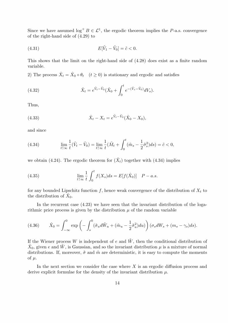
Since we have assumed log+B ∈ L1, the ergodic theorem implies the P -a.s. convergenceof the right-hand side of (4.29) to

(4.31) E[V1 − V0] = c < 0.

This shows that the limit on the right-hand side of (4.28) does exist as a finite randomvariable.

2) The process Xt = X0 θt (t ≥ 0) is stationary and ergodic and satisfies

(4.32) Xt = eVt−V0(X0 +

∫ t

0

e−(Vs−V0)dVs).

Thus,

(4.33) Xt −Xt = eVt−V0(X0 −X0),

and since

(4.34) limt↑∞

1

t(Vt − V0) = lim

t↑∞1

t(Mt +

∫ t

0

(ms −1

2σ2s)ds) = c < 0,

we obtain (4.24). The ergodic theorem for (Xt) together with (4.34) implies

(4.35) limt↑∞

1

t

∫ t

0

f(Xs)ds = E[f(X0)] P − a.s.

for any bounded Lipschitz function f , hence weak convergence of the distribution of Xt tothe distribution of X0.

In the recurrent case (4.23) we have seen that the invariant distribution of the loga-rithmic price process is given by the distribution µ of the random variable

(4.36) X0 =

∫ 0

−∞exp

(−∫ 0

s

(σudWu + (mu −1

2σ2u)du)

)(σsdWs + (ms − γs)ds).

If the Wiener process W is independent of e and W , then the conditional distribution ofX0, given e and W , is Gaussian, and so the invariant distribution µ is a mixture of normaldistributions. If, moreover, σ and m are deterministic, it is easy to compute the momentsof µ.

In the next section we consider the case where X is an ergodic diffusion process andderive explicit formulae for the density of the invariant distribution µ.

14

5. The invariant distribution

Let us now consider the special case of equation (4.1) where σ, m, σ,m, % are determin-istic constants. Thus, the process X is a Markovian diffusion with stochastic differentialequation

(5.1) dXt = Xt(σ dWt + m dt) + σ dWt +mdt

where W , W are Wiener processes with constant correlation %. Condition (4.23) reducesto

(5.2) m <1

2σ2,

and in this case X is an ergodic diffusion whose invariant distribution µ can be computedexplicitly.

(5.3) Theorem. Assume condition (5.2). If σ2 = 0 then m < 0, and the invariantdistribution is a normal distribution:

(5.4) µ = N(−mm,− σ

2

2m

).

If σ2 > 0 and |%| < 1 then the invariant distribution is given by the density

const·(σ2(1− %2) + (σx+ %σ)2

)−(1− mσ2 )

exp

(−2(%mσ −mσ)

σσ2√

1− %2arctan

σx+ %σ

σ√

1− %2

);(5.5)

for % = m = 0 this reduces to

(5.6) const·(

1 +σ2

σ2x2

)−(1− mσ2 )

For σ > 0 and |%| = 1 the density is

(5.7) const· (σx+ %σ)−2(1− m

σ2 ) exp

(2(%mσ −mσ)

σ2(σx+ %σ)

).

Proof. By (5.1), X satisfies the stochastic differential equation

(5.8) dXt = (mXt +m) dt+√σ2 + 2%σσXt + σ2X2

t dBt

for some Wiener process B. By Kolmogorov’s formula (see for instance Theorem IV.7 ofMandl (1968)), the density h of the invariant measure µ is given by

(5.9)(

log h(x))′

= −2%σσ −m+ (σ2 − m)x

σ2 + 2%σσx+ σ2x2

15

and therefore belongs to the family of Pearson type distributions. Integration leads to(5.4) – (5.7); see Johnson/Kotz (1970).

(5.10) Remark. The density in (5.5) is a Pearson type IV distribution; this is inter-esting since it seems that so far, “no common statistical distributions are of type IV”(Johnson/Kotz (1970)).

Let us now consider the case where m = 0 and % = 0 so that

(5.11) dXt = Xt(σ dWt + m dt) + σ dWt

with independent Wiener processes W and W . We can then think of W as an environmentof the diffusion which depends on some independent variable η.

(5.12) Remark. Equation (5.11) can be viewed as a special limiting case of the equation

(5.13) dXt = mtXt dt+ σ dWt

of an Ornstein-Uhlenbeck process in a random environment; cf. (3.14). To see this, supposethat the process (mt) in (5.13) is itself a recurrent Ornstein-Uhlenbeck process around thelevel m with variance v2 and drift parameter α < 0, defined as the pathwise solution of

(5.14) dmt = α(mt − m)dt+ v dWt

with respect to the independent Wiener process W . If v →∞ and v2

2α2 = σ2 is fixed, thenit is easy to check the pathwise convergence

(5.15) limv→∞

∫ t

0

ms(η) ds = σWt(η) + mt.

Thus, equation (5.13) is transformed into equation (5.11).

The strong solution (3.6) of equation (5.11) takes the form

(5.16) Xt = exp(σWt + (m− 1

2σ2)t

)(X0 +

∫ t

0

exp(− σWu − (m− 1

2σ2)u

)σ dWu

)

For a given environment η, X is therefore a Gaussian process with distribution

(5.17) N(Eη[X0] exp

(σWt(η) + (m− 1

2σ2)t

), Vt(η,Varη[X0])

)

at time t, where

(5.18) Vt(η, v2) = exp

(2σWt(η)+(2m− σ2)t

)(v2 +

∫ t

0

exp(−2σWs(η)−(2m− σ2)s

)ds).

16

The study of the diffusion (Vt) leads to an alternative proof of (5.5) and to an explicitrepresentation of µ in terms of a mixing measure on the variances.

(5.19) Theorem. Under condition (5.2) the process V = (Vt)t≥0 is a recurrent diffusionon [0,∞) whose invariant distribution ϑ is given by the density

(5.20) g(x) =1

Γ( 12 − m

σ2 )

(2σ2x)−( 1

2− mσ2 ) 1

xexp

(− σ2

2σ2x

).

The invariant distribution of X is given by

(5.21) µ =

∫ ∞

0

N (0, v2)ϑ(dv2).

Proof. By (5.18), V satisfies the stochastic differential equation

(5.22) dVt(η, v2) = 2Vt(η, v

2)σ dWt(η) +(σ2 + Vt(η, v

2)(2m+ σ2))dt.

By Kolmogorov’s formula, the density of the invariant measure for V is therefore given by

(5.23)(

log g(x))′

= −(log 4σ2x2)′ +2σ2 + 2x(2m+ σ2)

4σ2x2

which yields

g(x) = const·(4σ2x2)2m−3σ2

4σ2 exp

(− σ2

2σ2x

),

where the norming constant can be found by integration. Simplifying then leads to (5.20).To prove that µ in (5.21) is invariant for X, we consider the transition kernels

P ηt : N (c, v2) 7−→ N(ceσWt(η)+(m− 1

2 σ2)t, Vt(η, v

2)),

Pt =

∫P ηt ν(dη),

Qηt : v2 7−→ Vt(η, v2),

Qt =

∫Qηt ν(dη),

where ν denotes the distribution of the variable η. Then ϑQt = ϑ for each t, and we wantto show that µPt = µ for each t. For any bounded function f on IR, let

f(v2) =

∫

IR

f dN (0, v2).

17

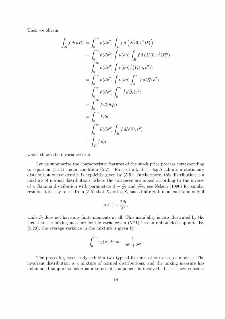
Then we obtain

∫

IR

f d(µPt) =

∫ ∞

0

ϑ(dv2)

∫

IR

f d(N (0, v2)Pt

)

=

∫ ∞

0

ϑ(dv2)

∫ν(dη)

∫

IR

f d(N (0, v2)P ηt

)

=

∫ ∞

0

ϑ(dv2)

∫ν(dη)f

(Vt(η, v

2))

=

∫ ∞

0

ϑ(dv2)

∫ν(dη)

∫ ∞

0

f dQηt (v2)

=

∫ ∞

0

ϑ(dv2)

∫ ∞

0

f dQt(v2)

=

∫ ∞

0

f d(ϑQt)

=

∫ ∞

0

f dϑ

=

∫ ∞

0

ϑ(dv2)

∫

IR

f dN (0, v2)

=

∫

IR

f dµ

which shows the invariance of µ.

Let us summarize the characteristic features of the stock price process correspondingto equation (5.11) under condition (5.2). First of all, X = logS admits a stationarydistribution whose density is explicitly given by (5.5). Furthermore, this distribution is amixture of normal distributions, where the variances are mixed according to the inverse

of a Gamma distribution with parameters 12 − m

σ2 and σ2

2σ2 ; see Nelson (1990) for similarresults. It is easy to see from (5.5) that Xt = logSt has a finite p-th moment if and only if

p < 1− 2m

σ2,

while St does not have any finite moments at all. This instability is also illustrated by thefact that the mixing measure for the variances in (5.21) has an unbounded support. By(5.20), the average variance in the mixture is given by

∫ ∞

0

xg(x) dx = − 1

2m+ σ2.

The preceding case study exhibits two typical features of our class of models: Theinvariant distribution is a mixture of normal distributions, and the mixing measure hasunbounded support as soon as a transient component is involved. Let us now consider

18

another case which illustrates these points and also shows that the mixing measure maybecome singular . The situation we shall examine arises if the random environment ofthe Ornstein-Uhlenbeck process in (3.14) and (5.13) is piecewise constant. More precisely,we consider the following situation: (βn)n∈IN is a sequence of i.i.d. random variables in-dependent of W with values in b1, ..., bm and distribution (p1, . . . , pm). The process(Xn)n=0,1,... is the Markov chain whose transition kernel is given by

P (x, ·) =m∑

j=1

pjPj(x, ·),

where

Pi(x, ·) = N(xeβi , σ2 e

2βi − 1

2βi

)

is the transition kernel of a discrete-time Ornstein-Uhlenbeck process. If βi = 0, we sete2βi−1

2βi= 1.

In order to find an invariant measure µ for the transition kernel P , we define a tran-sition kernel Q(u, dv) on (0,∞) by

Q(u, dv) =m∑

j=1

pjδAju+Bj (dv)

with

Aj = e2bj , Bj = σ2 e2bj − 1

2bj.

Intuitively, this corresponds to picking at random (according to p1, . . . , pm) one of the maffine linear mappings u 7→ Tju = Aju + Bj and then jumping from u to the image of uunder the chosen mapping. The question of existence of an invariant measure for randomiterations of affine linear maps which are contractive on average has been studied in detailby Barnsley/Elton (1988), and hence we obtain the following result.

(5.24) Theorem. Suppose that b1, . . . , bm and p1, . . . , pm satisfy the condition

(5.25) b =m∑

j=1

pjbj < 0.

Then the process X has a unique invariant distribution µ given by

(5.26) µ =

∫ ∞

0

N (0, c2)ϑ(dc2),

where ϑ is the unique invariant measure for Q on (0,∞) .

19

Proof. The existence and uniqueness of ϑ immediately follows from Theorem 1 of Barns-ley/Elton (1988) since (5.25) is equivalent to their condition of average contractivity, i.e.,

m∏

j=1

(Aj)pj < 1.

Thus it only remains to show that µ in (5.26) is invariant for P . But in analogy to theproof of (5.21),

µP =m∑

j=1

pj(µPj)

=m∑

j=1

pj

(∫ ∞

0

ϑ(du)N (0, u)Pj

)

=

∫ ∞

0

ϑ(du)m∑

j=1

pjN(

0, e2bju+ σ2 e2bj − 1

2bj

)

=

∫ ∞

0

ϑ(du)m∑

j=1

pj

∫ ∞

0

N (0, v)δAju+Bj (dv)

=

∫ ∞

0

ϑ(du)

∫ ∞

0

N (0, v)Q(u, dv)

=

∫ ∞

0

N (0, v) (ϑQ)(dv)

=

∫ ∞

0

N (0, v)ϑ(dv)

= µ,

and this completes the proof.

If we have additional information about the values b1, . . . , bm, we can also say moreabout the mixing measure ϑ. Let us suppose that (5.25) holds. If all bj are equal to some

b < 0, then ϑ is a point mass at −σ2

2b ; otherwise, ϑ is a continuous measure, and ϑ is eitherabsolutely continuous or singular. In fact, this is just Proposition 1 of Barnsley/Elton(1988). Furthermore, Theorem 3 of Barnsley/Elton (1988) tells us that supp ϑ = [d,∞)for some d ≥ 0, if there is at least one b` ≥ 0. Thus we see again that the existence of atleast one transient component is sufficient to destabilize the situation in the sense that themixing measure over the variances has unbounded support.

(5.27) Theorem. Suppose that b1, . . . , bm are all < 0.

1) If b1 < . . . < bm < 0, and if there exists some c > 0 such that

(5.28) 0 < B1 < A1c+B1 < B2 < A2c+B2 < . . . < Bm < Amc+Bm < c,

then supp ϑ ⊆ [0, c], and ϑ is singular.

20

2) Let fj = − σ2

2bjso that N (0, fj) is the invariant distribution of the recurrent Ornstein-

Uhlenbeck process with parameter bj < 0. Then

(5.29) supp ϑ ⊆[

min1≤j≤m

fj , max1≤j≤m

fj

].

Proof. 1) If we define the sets U = (0, c) and Vj = [Bj , Ajc+Bj ], then U is open, the

compact sets Vj are pairwise disjoint and satisfy Tj(U) ⊆ Vj and

m⋃

j=1

Vj ⊆ U by (5.28).

Thus 1) follows from Diaconis/Shahshahani (1986) since their condition (SC) is satisfied.

2) We may assume that b1 ≤ . . . ≤ bm < 0 so that f1 ≤ . . . ≤ fm. By Theorem 3.1 ofDiaconis/Shahshahani (1986), supp ϑ is the closure of the set

F =x∣∣x is fixed point of Ti1 . . . Tin for some n and i1, . . . , in ∈ 1, . . . ,m

.

Thus it is enough to show that all fixed points of all Ti1 . . . Tin lie in the interval [f1, fm].By an explicit computation, the fixed point of Ti1 . . . Tin is given by

f (n) =

n−1∑

k=0

Ai1 . . . AikBik+1

1−Ai1 . . . Ainso that

fm − f (n) =σ2Dn

1−Ai1 . . . Ainwhere

Dn = −n−1∑

k=0

Ai1 . . . AikAik+1

− 1

2bik+1

+1

2bm

(n∏

k=1

Aik − 1

).

We now show by induction that Dn ≥ 0 for all n. For n = 1,

D1 =1−Ai1

2

(1

bi1− 1

bm

)≥ 0

since Ai1 < 1 and bm ≥ bi1 . For n ≥ 1,

Dn+1 = Dn −Ai1 . . . AinAin+1 − 1

2bin+1

+1

2bm

(n+1∏

k=1

Aik −n∏

k=1

Aik

)

= Dn +n∏

k=1

Aik1−Ain+1

2

(1

bin+1

− 1

bm

)≥ 0

21

since Dn ≥ 0, 0 < Aik < 1 for all k and bm ≥ bin+1 . This implies that fm ≥ f (n) for all n,

and an analogous argument shows that f1 ≤ f (n) for all n.

Finally we remark that using 1) of Theorem (5.27), one can easily construct exampleswhere the measure ϑ is singular. For instance, we could take m = 2, b1 = −1, b2 = −0.5and any σ2 ≤ 0.5.

References

L. Bachelier (1900), “Theorie de la Speculation”, Ann. Sci. Ec. Norm. Sup. III-17, 21–86;english translation in “The Random Character of Stock Market Prices”(1964), ed. P. H.Cootner, MIT Press, Cambridge, Massachusetts, 17–78

M. F. Barnsley and J. H. Elton (1988), “A New Class of Markov Processes for ImageEncoding”, Advances in Applied Probability 20, 14–32

A. Bick (1987), “On the Consistency of the Black-Scholes Model with a General Equilib-rium Framework”, Journal of Financial and Quantitative Analysis 22, 259–275

P. Billingsley (1968), “Convergence of Probability Measures”, Wiley

F. Black (1986), “Noise”, Journal of Finance 41, 529–543

F. Black and R. Jones (1987), “Simplifying Portfolio Insurance”, Journal of Portfolio Man-agement 14, 48–51

F. Black and M. Scholes (1973), “The Pricing of Options and Corporate Liabilities”, Jour-nal of Political Economy 81, 637–659

A. Brandt (1986), “The Stochastic Equation Yn+1 = AnYn + Bn with Stationary Coeffi-cients”, Advances in Applied Probability 18, 211–220

P. L. Brockett and R. C. Witt (1991), “Relevant Distributions for Insurance Prices in anArbitrage Free Equilibrium”, Journal of Risk and Insurance 58, 13–29

P. Cagan (1956), “The Monetary Dynamics of Hyperinflation”, in “Studies in the Quantityof Money”, ed. M. Friedman, University of Chicago Press

R. H. Day and W. Huang (1989), “Bulls, Bears, and Market Sheep”, working paper, Uni-versity of Southern California

J. B. De Long, A. Shleifer, L. H. Summers and R. J. Waldmann (1990a), “Noise TraderRisk in Financial Markets”, Journal of Political Economy 98, 703–738

J. B. De Long, A. Shleifer, L. H. Summers and R. J. Waldmann (1990b), “Positive FeedbackInvestment Strategies and Destabilizing Rational Speculation”, Journal of Finance 44, 793–805

P. Diaconis and M. Shahshahani (1986), “Products of Random Matrices and ComputerImage Generation”, in “Random Matrices and Their Applications”, eds. J. E. Cohen,

22

H. Kesten and C. M. Newman, Contemporary Mathematics 50, American MathematicalSociety, 173–182

D. Duffie and P. Protter (1992), “From Discrete to Continuous Time Finance: Weak Con-vergence of the Financial Gain Process”, Mathematical Finance 2, 1–15

H. Follmer (1974), “Random Economies with Many Interacting Agents”, Journal of Math-ematical Economics 1, 51–62

H. Follmer (1991), “Probabilistic Aspects of Options”, SFB 303 discussion paper no. B–202, University of Bonn

J. A. Frankel and K. Froot (1986), “The Dollar as an Irrational Speculative Bubble: ATale of Fundamentalists and Chartists”, The Marcus Wallenberg Papers on InternationalFinance 1, 27–55

K. Froot and M. Obstfeld (1991), “Exchange Rate Dynamics under Stochastic RegimeShifts: A Unified Approach”, discussion paper no. 522, Centre for Economic Policy Re-search, London

C. Goodhart (1988), “The Foreign Exchange Market: A Random Walk with a DraggingAnchor”, Economica 55, 437–460

C. Gourieroux, J. J. Laffont and A. Monfort (1982), “Rational Expectations in DynamicLinear Models: Analysis of the Solutions”, Econometrica 50, 409–425

S. J. Grossman (1988), “An Analysis of the Implications for Stock and Futures PriceVolatility of Program Trading and Dynamic Hedging Strategies”, Journal of Business 61,275–298

O. D. Hart and D. M. Kreps (1986), “Price Destabilizing Speculation”, Journal of PoliticalEconomy 94, 927–952

J. Jacod and A. N. Shiryayev (1987), “Limit Theorems for Stochastic Processes”, Springer

N. L. Johnson and S. Kotz (1970), “Distributions in Statistics. Continuous UnivariateDistributions”, Houghton Mifflin, Boston

A. Kirman (1993), “Ants, Rationality and Recruitment”, Quarterly Journal of Economics(forthcoming)

D. Kreps (1982), “Multiperiod Securities and the Efficient Allocation of Risk: A Com-ment on the Black-Scholes Option Pricing Model”, in “The Economics of Uncertainty andInformation”, ed. J. McCall, University of Chicago Press, 203–232

T. G. Kurtz and P. Protter (1991a), “Characterizing the Weak Convergence of StochasticIntegrals”, in “Stochastic Analysis”, eds. M. T. Barlow and N. H. Bingham, CambridgeUniversity Press, 255–259

T. G. Kurtz and P. Protter (1991b), “Weak Limit Theorems for Stochastic Integrals andStochastic Differential Equations”, Annals of Probability 19, 1035–1070

23

D. W. Laidler (1985), “The Demand for Money”, Harper and Row, New York

P. Mandl (1968), “Analytical Treatment of One-Dimensional Markov Processes”, Springer

D. B. Nelson (1990), “ARCH Models as Diffusion Approximations”, Journal of Economet-rics 45, 7–38

A. Orlean and J.-M. Robin (1991), “Variability of Opinions and Speculative Dynamics onthe Market of a Storable Good”, preprint, Ecole Polytechnique, Paris

P. Protter (1990), “Stochastic Integration and Differential Equations. A New Approach”,Springer

P. A. Samuelson (1964), “Rational Theory of Warrant Pricing”, in “The Random Characterof Stock Market Prices”, ed. P. H. Cootner, MIT Press, Cambridge, Massachusetts, 506–525

P. A. Samuelson (1965), “Proof that Properly Anticipated Prices Fluctuate Randomly”,Industrial Management Review 6, 41–49

R. Shiller (1981), “Do Stock Prices Move Too Much to be Justified by Subsequent Changesin Dividends?”, American Economic Review 71, 421–436

L. SÃlominski (1989), “Stability of Strong Solutions of Stochastic Differential Equations”,Stochastic Processes and their Applications 31, 173–202

V. L. Smith, G. L. Suchanek and A. W. Williams (1988), “Bubbles, Crashes, and Endoge-nous Expectations in Experimental Spot Asset Markets”, Econometrica 56, 1119–1151

L. Summers (1986), “Does the Stock Market Rationally Reflect Fundamental Values”,Journal of Finance 41, 591–601

J. Tirole (1982), “On the Possibility of Speculation Under Rational Expectations”, Econo-metrica 50, 1163–1181

K. D. West (1988), “Bubbles, Fads and Stock Price Volatility Tests: A Partial Evaluation”,Journal of Finance 43, 639–660

N. Wiener (1923), “Differential-Space”, Journal of Mathematics and Physics 2, 131–174

24