a methodology to estimate supply chain cost of low demand
TRANSCRIPT

Rochester Institute of Technology Rochester Institute of Technology
RIT Scholar Works RIT Scholar Works
Theses
8-15-2015
A Methodology to Estimate Supply Chain Cost of Low Demand A Methodology to Estimate Supply Chain Cost of Low Demand
Parts Parts
Amey S. Mhapsekar
Follow this and additional works at: https://scholarworks.rit.edu/theses
Recommended Citation Recommended Citation Mhapsekar, Amey S., "A Methodology to Estimate Supply Chain Cost of Low Demand Parts" (2015). Thesis. Rochester Institute of Technology. Accessed from
This Thesis is brought to you for free and open access by RIT Scholar Works. It has been accepted for inclusion in Theses by an authorized administrator of RIT Scholar Works. For more information, please contact [email protected].
ROCHESTER INSTITUTE OF TECHNOLOGY
A METHODOLOGY TO ESTIMATE SUPPLY CHAIN COST OF LOW
DEMAND PARTS
Amey S. Mhapsekar [Pick the date]
Thesis submitted to the Faculty of the
Rochester Institute of Technology
In partial fulfillment of the requirements for the degree of
Master of Science in Industrial Engineering
Thesis Committee:
Dr. Scott Grasman
Dr. Denis Cormier
Department of Industrial and Systems Engineering
August 15, 2015
DEPARTMENT OF INDUSTRIAL AND SYSTEMS ENGINEERING
KATE GLEASON COLLEGE OF ENGINEERING
ROCHESTER INSTITUTE OF TECHNOLOGY
ROCHESTER, NEW YORK
CERTIFICATE OF APPROVAL
____________________
M.S. DEGREE THESIS
The M.S. Degree Thesis of Amey Mhapsekar
has been examined and approved by the
thesis committee as satisfactory for the
thesis requirement for the
Master of Science degree
Approved by:
__________________________________
Dr. Scott Grasman, Thesis Advisor
__________________________________
Dr. Denis Cormier, Committee Member

i
Acknowledgements
It is a great pleasure to present this report, a written testimony of real fruitful and invaluable research. I
take this opportunity to express my feeling of gratitude to the faculty of Industrial & Systems Engineering
Department at Rochester Institute of Technology for providing me with an opportunity to work on the
research topic of my interest. On completion of this course, I have personally experienced the
linkage between theoretical knowledge and its practical implication.
I am deeply indebted and would like to express my gratitude to Dr. Scott Grasman and Dr. Denis
Cormier for their guidance and profuse assistance during the research work. Their invaluable
support makes this thesis a successful work.
I would like to express my sincere thanks to Dr. Michael Hewitt, Dr. Ruben Proano and
Professor John Kaemmerlen who gave me invaluable guidance during this research period.
Last, but not the least, I would like to thank my family for their continuous love and support for my
education and my friends, Anirudha, Anshul, Atul, Chaitanya, Mugdha, Nisarth and Vinayak, for making
this journey so memorable. I was able to learn and enjoy my learning period as a result of their
unconditional backing towards my learning ventures.

ii
Abstract
As according to the Magnuson-Moss Warranty Act, automobile manufacturers are required to
provide spare parts for any model they sell, for a minimum span of 10 years. In the automobile/
aviation industry, the demand for replacement parts is generally met using conventional
manufacturing processes such as injection molding (IM) and stocking parts in warehouses. IM
proves economical when the demand is high and continuous. The demand for replacement parts
is generally low and intermittent and stocking parts in inventory to meet future demands proves
expensive and the possibility of stock-outs or parts going obsolete is high.
Rapid Manufacturing (RM) is an additive manufacturing technique that prints parts without the
need of tools, unlike conventional manufacturing processes. Thus, it saves on the tooling cost,
time to make the mold, and the need to stock various parts in order to meet the intermittent
demand. There is a need for an alternative approach to meet low volume intermittent demands,
and the Just in Time (JIT) production strategy incorporating RM serves as an option. In JIT,
production starts when a demand is received from the customer. It also gives the Original
Equipment Manufacturer (OEM) an option to make parts on the demand site, eliminating
transportation and inventory holding costs.
The objective of this thesis is to develop a decision making framework to determine the
economical supply chain strategy to meet the demand for replacement parts. The supply chain
strategies considered are in-house manufacturing by the RM process called Selective Laser
Sintering (SLS) in a JIT production environment, and stocking parts in centralized warehouses
manufactured by IM to meet future demands. A mixed integer programming (MIP) model has
been formulated to determine the unit cost of parts for the supply chain strategies under
consideration. The results from the model are used to determine the significant part parameters
affecting the cost of manufacturing by SLS using Regression Analysis. Based on the results,
material volume and height of the part proved to be significant factors and a regression equation
has been derived and validated for estimating the unit supply chain cost of parts manufactured by
SLS.
iii
Table of Contents
List of Acronyms .......................................................................................................................................... vii
List of Notations ......................................................................................................................................... viii
Chapter 1. INTRODUCTION ..................................................................................................................... 1
1.1 Background on Rapid Manufacturing ........................................................................................... 1
1.2 Problems Faced by OEMs and Options Available With the Use of Rapid Manufacturing ............ 3
1.3 Thesis Objectives ........................................................................................................................... 5
Chapter 2. LITERATURE REVIEW ............................................................................................................. 7
2.1 Supply Chain Theories and Strategies ........................................................................................... 7
2.1.1 Supply chain strategies to meet uncertain demands ........................................................... 7
2.1.2 Supply chain strategies for replacement parts incorporating rapid manufacturing ............ 8
2.2 Cost Analysis of Parts .................................................................................................................... 9
Chapter 3. PROBLEM DEFINITION ......................................................................................................... 16
Chapter 4. MATHEMATICAL FORMULATION ........................................................................................ 17
4.1 Cost Functions for SLS ................................................................................................................. 18
4.1.1 Machine usage cost............................................................................................................. 18
4.1.2 Energy consumption cost .................................................................................................... 18
4.1.3 Material cost ....................................................................................................................... 19
4.1.4 Labor cost ............................................................................................................................ 19
4.2 Cost Functions for IM .................................................................................................................. 19
4.2.1 Machine usage cost............................................................................................................. 20
4.2.2 Energy consumption cost .................................................................................................... 20
4.2.3 Tooling cost ......................................................................................................................... 20
4.2.4 Material cost ....................................................................................................................... 20
4.2.5 Labor cost ............................................................................................................................ 21
4.2.6 Storage cost......................................................................................................................... 21
4.2.7 Inventory holding cost ........................................................................................................ 21
4.2.8 Transportation cost ............................................................................................................. 21
Chapter 5. RESEARCH METHODOLOGY ................................................................................................ 34
5.1 Type of Part ................................................................................................................................. 34
5.2 Process Capability and Machine Specification ............................................................................ 37

iv
5.3 Demand Quantity ........................................................................................................................ 38
5.4 Cost and Time Parameters .......................................................................................................... 38
5.4.1 Material cost ....................................................................................................................... 38
5.4.2 Machine cost ....................................................................................................................... 39
5.4.3 Tool cost .............................................................................................................................. 39
5.4.4 Energy, labor and inventory costs ....................................................................................... 40
5.4.5 Transportation .................................................................................................................... 40
5.4.6 Time .................................................................................................................................... 41
Chapter 6. EXPERIMENTAL RESULTS & ANALYSIS ................................................................................. 42
6.1 Preliminary Experimental Results ............................................................................................... 42
6.2 Determining Significant Factors and Deriving Regression Equation for Unit Supply Chain Cost of
SLS .................................................................................................................................................... 46
6.3 Validation Experiments for the Regression Equation ....................................................................... 50
Chapter 7. CONCLUSIONS & FUTURE WORK ........................................................................................ 57
REFERENCES ................................................................................................................................................ 58
Appendix A: Results from the mathematical model for preliminary experiments..................................... 60
Appendix B: Results from the mathematical model for experimental setup in Table 17 .......................... 62
Appendix C: Minitab Output ....................................................................................................................... 63
Minitab Output for Full model ................................................................................................................ 63
Minitab Output for Reduced model ....................................................................................................... 64
Appendix D: Results from the mathematical model for experimental setup in Table 18 .......................... 66
v
List of Figures
Figure 1: Cost comparison for small part (Hopkinson & Dickens, 2003) .................................................... 10
Figure 2: Cost comparison for large part (Hopkinson & Dicknes, 2003) ..................................................... 11
Figure 3: Production curve for the lever (M. Ruffo et al., 2006) ................................................................ 12
Figure 4: Comparison between production curves for the spring clip in single part and mixed production
scenarios (M. Ruffo & Hague, 2007) ........................................................................................................... 13
Figure 5: Total cost of the lamp holder manufactured by IM for different production volumes (Atzeni et
al., 2010) ..................................................................................................................................................... 14
Figure 6: Total cost of the lamp holder manufactured by SLS for the two EOS machines (Atzeni et al.,
2010) ........................................................................................................................................................... 14
Figure 7 : Bracket (GRABCAD, 2013a) ......................................................................................................... 34
Figure 8 : Gear (GRABCAD, 2013b) ............................................................................................................. 35
Figure 9 : Horn (GRABCAD, 2013c) ............................................................................................................. 35
Figure 10 : Impeller (GRABCAD, 2013d) ...................................................................................................... 35
Figure 11 : Plastic Impeller (GRABCAD, 2013e) .......................................................................................... 36
Figure 12 : Spur gear (GRABCAD, 2013f)..................................................................................................... 36
Figure 13: Distribution of costs for low demand manufactured by IM ...................................................... 43
Figure 14: Distribution of costs for medium demand manufactured by IM ............................................... 43
Figure 15: Distribution of costs for high demand manufactured by IM ..................................................... 44
Figure 16: Distribution of costs for low demand manufactured by SLS ..................................................... 45
Figure 17: Distribution of costs for medium demand manufactured by SLS .............................................. 45
Figure 18: Distribution of costs for high demand manufactured by SLS .................................................... 45
Figure 19: Analysis of variance for the full regression model ..................................................................... 47
Figure 20: Analysis of variance for the reduced model .............................................................................. 48
Figure 21: Residual Plots for unit supply chain cost for SLS ....................................................................... 49
Figure 22: Normality test for residuals from unit supply chain cost for SLS ............................................... 49
Figure 23: Regression equation for predicting unit supply chain cost of parts manufactured in-house
using SLS ...................................................................................................................................................... 49
Figure 24: Box plot of material volume vs supply chain strategy ............................................................... 54
Figure 25: Box plot of bounding box height vs supply chain strategy ........................................................ 55
Figure 26: Box plot of bounding box cross section vs supply chain strategy .............................................. 55
Figure 27: Box plot of material volume vs supply chain strategy when tool cost reduces ........................ 56
Figure 28: Box plot of material volume vs supply chain strategy when tool cost increase ........................ 56

vi
List of Tables
Table 1: Comparison between Rapid Manufacturing and Injection Molding ............................................... 5
Table 2: Supply Chain strategies for service parts ........................................................................................ 9
Table 3 : Part Complexity ............................................................................................................................ 36
Table 4: Actual and bounding box dimensions of parts .............................................................................. 37
Table 5: Process capability of Injection Molding (Custompart.net, 2013a) ................................................ 37
Table 6: Process capability of SLS (Custompart.net, 2013b)....................................................................... 37
Table 7: Sinterstation Pro 140 machine specifications (Systems, 2007) .................................................... 38
Table 8: Demand levels ............................................................................................................................... 38
Table 9: Material cost and specification(Corporation, 2010) (Custompart.net, 2013a) ............................ 39
Table 10: Machine cost and specification (Corporation, 2010) .................................................................. 39
Table 11: Tool Cost (Custompart.net, 2013a) ............................................................................................. 40
Table 12: Rate of Energy, Labor and Storage .............................................................................................. 40
Table 13: Rate of shipping........................................................................................................................... 40
Table 14: Unit mold cost of parts ................................................................................................................ 42
Table 15: Unit supply chain cost of parts manufactured by IM .................................................................. 43
Table 16: Unit supply chain cost of parts manufactured in-house by SLS .................................................. 44
Table 17: Levels of part specifications with respect to machine specifications ......................................... 47
Table 18: Setup for validation experiments ................................................................................................ 50
Table 19: Summary of validation experiments ........................................................................................... 51
Table 20: Unit supply chain cost for the two supply chain strategies under consideration ....................... 53
vii
List of Acronyms
viii
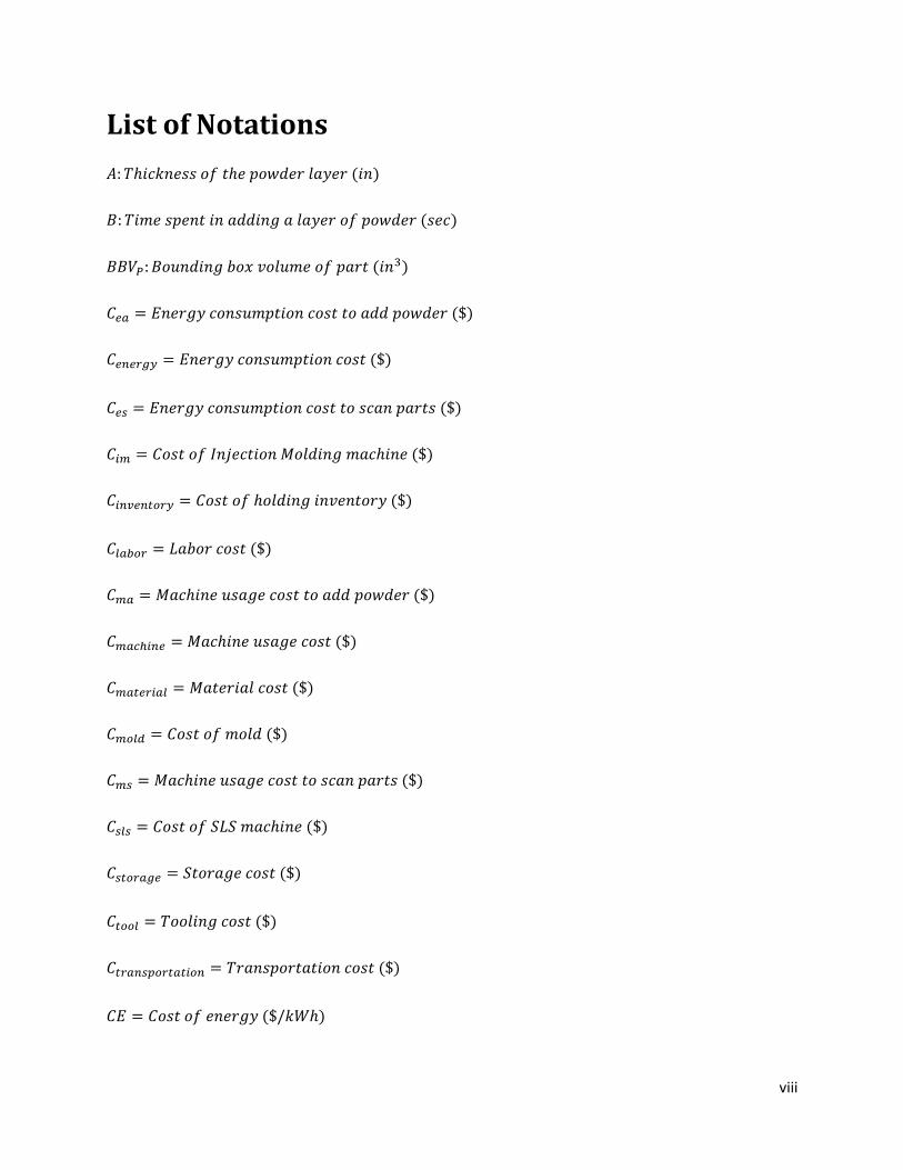
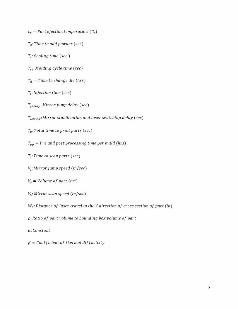
List of Notations

ix
x
1
Chapter 1. INTRODUCTION
1.1 Background on Rapid Manufacturing
Rapid Manufacturing (RM) is a manufacturing process that uses Layer Manufacturing
Techniques (LMT) to build 3D products that are part of assemblies or the final product. The
material cost, cycle time and capital investment for RM machines is generally high compared to
conventional manufacturing processes such as Injection Molding (IM), making it undesirable for
manufacturing of products in high or medium volumes. Hopkinson & Dickens (2001) state that
the advantages of RM over conventional processes come in the form of zero tool cost, reduced
lead time of making the tool, and freedom in product design proves instrumental in accepting the
potential benefits to be gained by employing RM.
The prime difference between RM and the traditional machining manufacturing techniques is
that RM is not a subtractive manufacturing process, i.e., it does not involve removal of material
from the part, thus resulting in minimal material wastage. It is referred to as an Additive
manufacturing process. There are many sectors in which the RM technology has been
successfully implemented. Chandra et al. (2005) provides an example with people affected by
facial deformity, which can be congenital or accidental, needing rehabilitation of the face. RM
has been used to create an impression of the patient’s face in addition to the mask which would
fit the impression, making it appropriate for the patient to use the mask as per the facial
geometry. This is difficult for any conventional manufacturing process.
Rapid Prototyping (RP) and RM techniques provide designers the freedom to change or make
modifications in the CAD file at the last moment to facilitate production of parts of any size, any
geometry and with reduced time required to make the parts. Wannarumon & Bohez (2004)
pointed out the inability of conventional jewelry manufacturing processes such as investment
casting to provide these benefits. Berman (2012) studied the application of RM to the footwear
industry which allows customization of footwear as per requirements of size, design and color. It
eliminates the constraints of conventional manufacturing mechanisms such as the need for
cutting of materials and new organization of the work process in manufacturing.
2
The traditional methodology of creating dental implants is to create a plaster model of an oral
impression, then hand carve a wax pattern of how the repaired tooth will look, cast it, and then
add a porcelain or ceramic veneer to it. RM substitutes this method by taking a digital scan of the
mouth, and then using a CAD program to design the prosthesis. This file is then outputted in
STL format, imported into the RM machine which can build the wax mold or if required the
tooth itself ("Additive Fabrication Transforms Dental Labs," 2008).
One drawback of some RM processes is the relatively inferior material properties of parts
compared to the material properties of those manufactured using traditional processes. In order to
get over this drawback and have material properties of parts as good as the ones obtained using
traditional manufacturing processes, there has been customized use of materials to suit the need
of industries which demand high material properties. This comes at a high cost. Rocketdyne
Propulsion and Power has successfully used SLS technology to custom make titanium alloy parts
for NASA’s space shuttles to withstand high temperature. These parts have already been used
successfully in orbit ("The solid future of rapid prototyping," 2001).
RM has been successfully implemented in manufacturing by organizations such as Boeing,
NASA, Align Technologies, BMW and Paramount PDS. Boeing's Rocketdyne propulsion and
power section have used SLS to manufacture low volumes of parts in space labs and space
shuttles ("3D Printing Industry, Explore the Many Uses of FDM | Stratasys," 2014). BMW has
adopted RM for manufacturing jigs & fixtures used for assembly and test operations. These jigs
and fixtures are built from Acrylonitrile Butadiene Styrene (ABS) using the Fused Deposition
Modeling (FDM) process and are much lighter and ergonomically superior compared to the
traditionally manufactured jigs and fixtures machined from aluminum and polyamide. BMW also
uses RM to create patterns for sand casting ("Direct Digital Manufacturing AT BMW," 2015).
Paramount PDS, a product development and RM company in the USA, uses a material which is
certified and accredited by independent laboratories complying with regulations to flammability,
smoke generation and smoke toxicity. They manufacture flight hardware components for
commercial luxury aircraft that enables the aircraft company to cut down on lead times and
eliminate tool cost ("Paramount PDS Delivers Flight-Ready Parts for Commercial Aircraft with
Rapid Manufacturing with EOS's Flame Retardant Laser-Sintering Material," 2007).
3
1.2 Problems Faced by OEMs and Options Available With the
Use of Rapid Manufacturing
Hasan & Rennie (2008) identified the potential of a RM supply chain in the spare parts industry.
The authors addressed the frequently faced problems by the aerospace and automotive industry
of unavailability of spare parts. Conventional manufacturing processes such as IM depend on
economies of scale for profit, resulting in manufacturing in large quantities to meet future
demands. It is difficult to stock all the parts in inventory due to the variety of parts that go into
the making of an aircraft or an automobile. Also, many of the parts are not frequently needed,
and stocking them proves expensive due to high inventory holding cost. The unavailability of
replacement parts keeps the aircrafts grounded, which hurts the airline due to loss of business.
The OEM is left with a difficult question to answer as to which parts to stock in inventory and
how much to stock.
Pérès & Noyes (2006) addressed the problems faced in the management of spare parts in
‘isolated systems’. The supply of parts is made difficult due to the specific environment not
being suitable for storing parts due to space constraints. The authors investigated the idea of
creating parts on the spot as per demand, and introduced the concept of e-logistics support. They
described and classified the various RM techniques and the benefits from using these techniques
in remote systems. They also discussed studies based on industrial cases representing different
modes of system isolation.
Meadows (1997) addressed the problem faced by the defense department in acquiring spare parts
for aircrafts, ships and trucks because many of the systems currently in operation were built
decades ago. Platforms such as the B-52 bomber, KC-135 tanker aircraft and the C-130 cargo
plane which were built in the mid 90’s are expected to remain operational for the foreseeable
future. The lack of spare parts to maintain them would result in stoppage in their usage. In
addition to these aging systems, even the new F-22 fighter aircraft, the B-2 stealth bomber and
the Navy’s F/A-18 have been found to face lack of spare parts. The unavailability of parts not
only leads to longer logistics cycles for weapons systems but also forces operators to remove
parts from operational platforms to replace missing ones in other systems. It is observed that
companies with both government and commercial customers have shut down their military lines
4
to pursue higher demands and more profitable opportunities, as the military was not ordering in
sufficient quantities to justify keeping production lines open.
The ‘make to stock’ supply chain strategy in which large batches of parts are manufactured,
stocked at centrally located warehouses, and supplied on demand has traditionally been used.
The positive of employing this strategy is the low lead time of meeting demands. However, the
negatives can outnumber the positives of this strategy in some cases. The inventory holding cost
is high, the transportation costs from a centralized location are high, and there is always a risk of
stock outs or parts going obsolete if there is no demand. Forecasting is the basis of employing
this strategy and can result in either overstock or stock out due to varying demand.
The OEM has to shoulder the responsibility for providing speedy service along with
minimization of inventory cost. Stocking parts in inventory is a risk as these parts may never be
used, and the OEM will have to bear the obsolescence cost. The uncertainty of demand also
poses a threat to the suppliers of these OEM’s as they have to bear the cost of raw material
produced at their end. The cost of holding inventory is very high as it adds the cost of surplus
parts to the capital investment made by the organization. RM technology is an alternative to the
conventional manufacturing processes in cases of low demand. The material cost for
manufacturing parts by RM is high, but it eliminates the high inventory cost and the risk of stock
outs.
The costs associated with the parts vary depending on the process used to manufacture them; the
cost of delivering parts depends on the facility location and mode of transportation. If the parts
are manufactured by conventional processes such as IM, the costs applicable to these parts are in
the form of tool costs, material costs, machining costs, labor costs, inventory costs and
transportation costs from central warehouses or distribution centers to the desired location. RM
allows freedom in the design of the part as no additional tooling or machining is required in case
of a complex geometry which is a drawback of traditional processes.
The use of RM would prove economical and feasible when the demand quantity is low. The
inventory cost gets eliminated completely. The transportation cost may apply if the parts are
being manufactured at a centralized location, but it gets eliminated if the RM is done at the point
5
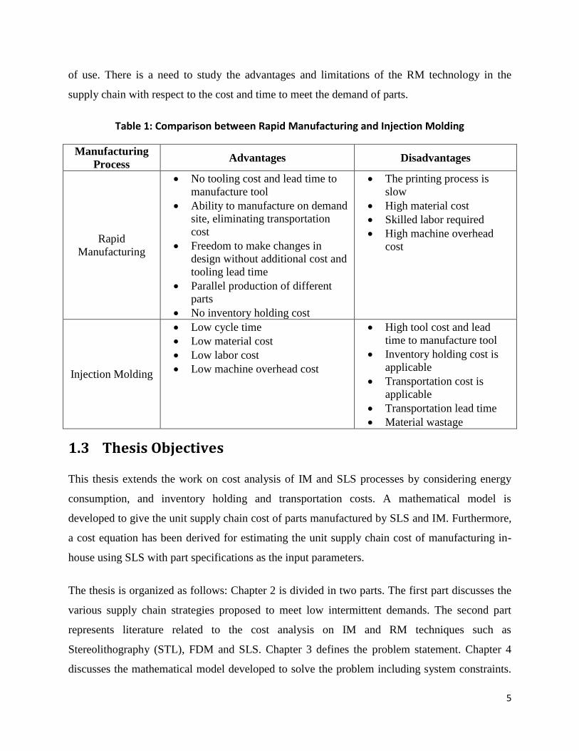
of use. There is a need to study the advantages and limitations of the RM technology in the
supply chain with respect to the cost and time to meet the demand of parts.
Table 1: Comparison between Rapid Manufacturing and Injection Molding
Manufacturing
Process Advantages Disadvantages
Rapid
Manufacturing
No tooling cost and lead time to
manufacture tool
Ability to manufacture on demand
site, eliminating transportation
cost
Freedom to make changes in
design without additional cost and
tooling lead time
Parallel production of different
parts
No inventory holding cost
The printing process is
slow
High material cost
Skilled labor required
High machine overhead
cost
Injection Molding
Low cycle time
Low material cost
Low labor cost
Low machine overhead cost
High tool cost and lead
time to manufacture tool
Inventory holding cost is
applicable
Transportation cost is
applicable
Transportation lead time
Material wastage
1.3 Thesis Objectives
This thesis extends the work on cost analysis of IM and SLS processes by considering energy
consumption, and inventory holding and transportation costs. A mathematical model is
developed to give the unit supply chain cost of parts manufactured by SLS and IM. Furthermore,
a cost equation has been derived for estimating the unit supply chain cost of manufacturing in-
house using SLS with part specifications as the input parameters.
The thesis is organized as follows: Chapter 2 is divided in two parts. The first part discusses the
various supply chain strategies proposed to meet low intermittent demands. The second part
represents literature related to the cost analysis on IM and RM techniques such as
Stereolithography (STL), FDM and SLS. Chapter 3 defines the problem statement. Chapter 4
discusses the mathematical model developed to solve the problem including system constraints.

6
Chapter 5 describes the selection of parameters and their values as input to the mathematical
model. Chapter 6 presents numerical experiments performed using the mathematical model,
deriving the equation to predict the unit supply chain cost of parts manufactured in-house using
SLS and validating the results. Finally, Chapter 7 discusses the conclusions and future work.

7
Chapter 2. LITERATURE REVIEW
The first section of the literature review presents a study on various supply chain theories and
strategies. The second section presents work related to the cost analysis of plastic parts
manufactured using IM and RM processes such as STL, FDM and SLS.
2.1 Supply Chain Theories and Strategies
There has been extensive research in the field of Supply Chain Management addressing
problems faced in manufacturing. This literature review focuses on the Supply Chain theories
and strategies addressing uncertain demand and replacement parts incorporating RM.
2.1.1 Supply chain strategies to meet uncertain demands
Fisher (1997) introduced the concept of matching supply chain strategies to the right level of
demand uncertainty of a product in case of high obsolescence and/or stock out cost. The author
summarized that the critical decisions to be made are not always about minimizing production
and distribution costs but about positioning inventory and available production capacity in order
to meet uncertain demand. Similarly, the suppliers should be chosen not only for their low cost
but for their flexibility and speed as well. Holmström, Louhiluoto, Vasara, & Hoover (2001)
suggested that in order to minimize delivery times and to fulfill orders, a wide range of products
have to be stocked in inventory resulting in large inventory costs. The authors discussed that
suppliers can offer value to customers and improve their operations without weighing the
benefits of customer service against cost by changing the demand supply chain.
Christopher (2000) mentioned that short product life cycle, global economic and competitive
forces create uncertainty, turning the market turbulent and volatile. The author suggested that
‘agility’ is the key to surviving in this scenario by creating responsive supply chains. The author
made a distinction between the philosophies of ‘lean’ and ‘agility’ and pointed out that the
challenge to supply chain management in such a volatile market is to develop lean strategies up
to the decoupling point and agile strategies beyond that.
Christopher & Towill (2001) suggested that in some markets, meeting customer expectation by
getting the right product at the right price and at the right time is critical for competitive success.
8
The authors mentioned that the lean philosophy is powerful when the winning criterion is cost
but when customer service is the winning criteria, agility is the way to go. The authors explored
the combination of lean and agility as a hybrid strategy to create a cost effective and responsive
supply chain. The authors proposed three ways in which the lean and agile philosophies could
co-exist; the Pareto approach, the de-coupling point approach and the separation of base and
surge demands.
2.1.2 Supply chain strategies for replacement parts incorporating rapid
manufacturing
Huiskonen (2001a) addressed the requirements for planning the logistics of spare parts
differently from other materials due to sporadic demand, difficulty in forecasting, and high part
prices. The author studied the effects of various operational control characteristics such as
criticality, specificity, demand pattern and value of spare parts on the logistics system design
(service strategy, supply structure, supply chain relationship and inventory control system).
The impact of the use of RM on the supply chain management of replacement parts in the
aircraft and automotive industry has been of interest to many supply chain specialists such as
Walter, Holmstrom, & Yrjola (2004) and Holmstrom (2010). Walter et al. (2004) and
Holmstrom (2010) addressed supply chains in which both manufacturing and distribution are
challenging. The spare parts supply in the aircraft industry served a perfect example for their
study because of the rapid repairs and maintenance required to avoid losses due to aircraft being
grounded. They studied the problems faced by aircraft OEM’s in dealing with the demand for
replacement parts. Their study found out that the major concern of the OEM is the wide range of
parts that an aircraft is made up of and the impracticality of storing all parts in inventory due to
the high inventory holding cost and uncertain demand. They also pointed out the issue of parts
going obsolete if stocked to cover the entire life cycle, given the long life cycle of these parts in
addition to the declining service lives of aircrafts. They also highlighted the high cost and time
required for manufacturing parts on demand using conventional manufacturing processes such as
IM. They analyzed the drawback of having both frequently and infrequently required parts stored
in inventory and delivered as per the demand from centralized warehouses of the OEM to the
demand site.

9
The various proposed supply chain strategies to deal with the problem of service parts is
tabulated below:
Table 2: Supply Chain strategies for service parts
Author Strategy
Jan Holmstrom, 2010
Christopher & Towill, 2001 Centralized RM machine for slow moving type B and C parts
Jan Holmstrom, 2010 Centralized warehousing and centralized RM machine
Wohlers & Grimm, 2002 Centralized multiple RM machines
Pérès & Noyes, 2006 Demand site RM machine
Ruffo, Tuck, & Hague (2007) carried out an analysis to decide if an OEM should invest directly
in an RM machine for employing the distributed RM supply chain strategy or outsource
infrequently needed replacement parts to suppliers having expertise in the RM technology. The
authors summarized the pros and cons of make or buy decisions followed by the effect of RM
technology on the outsourcing decision. The authors focused on two strategies for their analysis,
both showing the cost effectiveness of in-house manufacturing over outsourcing.
In-house manufacturing or outsourcing using traditional manufacturing resources.
In-house manufacturing using RM if resources and skills are available or outsource to
RM suppliers.
Huiskonen (2001b) categorized spare parts on the basis of their criticality (high or low) and
specificity (standard or customized). They suggested that categorization along these lines is more
efficient in managing the supply chain of spare parts compared to the classification of these parts
on the basis of profitability (ABC) as per the Pareto rule. The author however did not validate his
analysis with data.
2.2 Cost Analysis of Parts
A cost analysis was performed by Hopkinson & Dickens (2001) in which they compared the
manufacturing cost per part required to produce four different parts varying in size, by IM and
SLS. The cost parameters considered for the analysis were fixed machine costs, and variables
costs including machine operation cost, material cost and tooling cost. The material from which
the parts were to be manufactured was selected to be polypropylene. The results showed that the
10
unit cost of the parts manufactured by SLS was constant irrespective of the number of parts
manufactured. The authors inferred that small parts with high geometric complexity made in low
volumes were best suited for manufacturing using SLS technology.
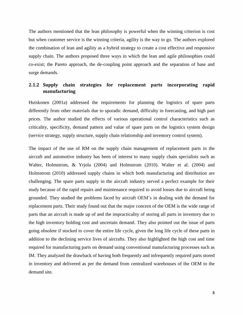
Another cost analysis was performed by Hopkinson & Dicknes (2003) to compare the unit cost
of parts manufactured in a time frame of one year using IM and the three RM processes SLA,
FDM, and SLS. The analysis was carried out on two plastic components differing in size. The
cost parameters considered for the analysis were machine cost, material cost, labor cost and
tooling cost. It was observed that the total number of parts manufactured in a year by each
process differed as a result of different production speeds, with FDM being the slowest followed
by SLA, and then SLS. The contribution of the machine cost, material cost and labor cost to the
total cost were different for the three RM processes. The contribution of machine cost to the total
cost of part manufactured by SLA and FDM was highest followed by material cost. On the
contrary, the material cost was the highest contributor to the total cost of part manufactured by
SLS, because the unsintered material is not reused. The machine cost for SLS was lower
compared to SLA and FDM as the machine was capable of building a higher number of parts due
to a high build rate. It was observed that the cost per part was highest for SLA followed by FDM
and SLS. Figure 1 shows that for the small part, the production quantity at which IM is cheaper
was greater for SLS compared to the SLA and FDM processes. Figure 2 shows that for the large
part, the production quantity at which IM is cheaper was greater for FDM compared to SLA.
Figure 1: Cost comparison for small part (Hopkinson & Dickens, 2003)
11
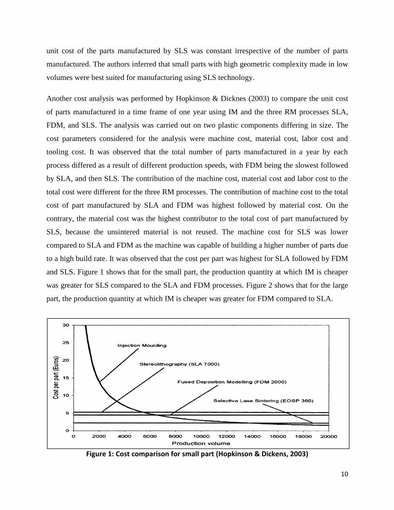
Figure 2: Cost comparison for large part (Hopkinson & Dicknes, 2003)
The above graphs infer that the cost per part is constant irrespective of the production quantity
for SLA, FDM and SLS respectively; whereas the cost per part decreases in case of IM as the
tool cost gets amortized by the production quantity. The comparisons proved that IM is a cheaper
process for high production volumes. It was observed that apart from low production volumes,
the production rate and material cost made it difficult to opt for RM for large parts. When the
manufacture of parts with complex geometries was analyzed, injection molded parts required
additional machining to meet the part geometry, adding to the final cost of parts. Thus, small
parts having complex geometries and small production volumes were deemed to be best suited
for RM process. The above analysis is a good approximation when the RM machines are
manufacturing copies of the same part and the production volume is high.
Another cost model was developed by Ruffo, Tuck, & Hague (2006) in which the authors
considered the impact of investments and overheads on the per part cost. The authors categorized
costs as direct and indirect in which material cost was considered to be direct and machine
absorption, labor and maintenance costs were considered to be indirect costs. They assigned
indirect costs to the parts on a machine working time basis. The authors assumed the machine
utilization to be 57% compared to 90% assumed by Hopkinson & Dicknes (2003). Their results
showed a saw tooth shaped curve which had deflections for low production volumes unlike the
constant cost from Hopkinson & Dicknes (2003). The cost curve had a tendency to change
whenever a row in the x-direction was used, a new layer was required, or when a new bed was

12
required due to the filling of machine bed space as shown in Figure 3. Part size and the packing
ratio were drivers of the cost model and influenced the initial transition and the stabilized value
of the curve. The authors inferred that large parts occupy a large portion of the machine bed
resulting in the cost being split between fewer parts. The packing ratio, which is affected by part
size, influences both build time and material waste.
Figure 3: Production curve for the lever (M. Ruffo et al., 2006)
A method for cost calculation of mixed parts in the same build envelops, referred to as ‘Parallel
Production’, was developed by Ruffo & Hague (2007). They proposed three different
mathematical models for the cost estimation of the SLS process and compared them through a
case study. Their proposed approaches were as follows:
Cost of a single part was first calculated as a fraction of the total cost using the ratio
between volume of the part and the total volume of production. In their previous
research, Ruffo et al. (2006) demonstrated that the part volume, considered singularly, is
not enough for time and cost estimation. Thus, they proposed a different solution.
An alternate solution proposed calculating cost of a single part by splitting the full build
cost into different parts placed on the machine bed. The error with this approach was the
poor packing ratio used for calculation due to the machine bed being partially empty.
Finally, they proposed calculating cost of a single part based on the cost of a part built in
a high volume production.
13
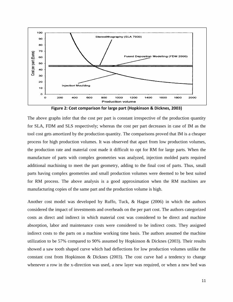
The authors tested the third methodology in two scenarios, one in which the machine builds
copies of the same part, and the other in which the machine employs parallel production of
mixed components. Figure 4 displays their results which suggest that when different components
are efficiently mixed in the building space, the cost of each component decreases.
Figure 4: Comparison between production curves for the spring clip in single part and mixed
production scenarios (M. Ruffo & Hague, 2007)
A study on the interrelation between redesign and cost estimation was carried out by Atzeni,
Iuliano, Minetola, & Salmi (2010). The authors pointed out that a remarkable cost reduction is
obtained when the component shape is modified to exploit the advantages of RM. The authors
considered material cost and processing costs (part design and testing cost, machine cost, labor
cost, post-processing cost) for RM and mold, assembly, machine, material and labor costs for
IM. They didn’t consider administrative overhead, energy, space rental or ancillary equipment
costs. The authors compared the cost per part for IM against production volumes ranging 5,000
to 500,000 parts. They compared the per part cost for two different SLS machines; the P390
which has a smaller bed volume compared to the P730 machine. A sensitivity analysis was
carried out varying each cost parameter for both IM and SLS. It was observed that the mold cost
was the sole significant contributor to the unit cost of part manufactured by IM, whereas machine
and material cost was the significant contributor to the unit cost of parts manufactured by SLS.
Figure 5 summarizes the contribution of mold cost, assembly cost, machine cost, material cost
and labor cost per part for different production volumes. Figure 6 summarizes the contribution of

14
machine, material, labor and assembly cost per part manufactured using the two SLS machines
under consideration.
Figure 5: Total cost of the lamp holder manufactured by IM for different production volumes
(Atzeni et al., 2010)
Figure 6: Total cost of the lamp holder manufactured by SLS for the two EOS machines (Atzeni
et al., 2010)
The studies carried out by Hopkinson & Dickens (2001) and Hopkinson & Dickens (2003) have
focused on determining the crossover point in which one switches from RM to IM in terms of
unit cost with respect to production volume for the parts under consideration. The research
carried out by Ruffo, Tuck & Hague (2006) focused on determining part size and the packing
ratio as the factors affecting the unit cost of part. Ruffo & Hague (2007) extended their research

15
in determining the effect of parallel production on the unit cost of parts. A quantitative analysis
on the supply chain cost of parts considering the two manufacturing processes RM and IM hasn’t
been done. Also, the part specifications affecting the unit cost of part manufactured by RM
hasn’t been looked into.
16
Chapter 3. PROBLEM DEFINITION
Consider an organization ABC that receives demand for a variety of parts in different quantities.
At present, ABC has been fulfilling its customer’s demand by delivering parts stocked in their
central warehouse that were manufactured by IM. ABC has been in situations where either the
stocked parts have gone obsolete resulting in obsolescence cost, or they ran short on parts. The
organization is looking for an alternate approach and is planning to adopt the JIT production
strategy incorporating SLS wherein they could start production only after a demand is received
from the customer. This production strategy would help them reduce the risk of bearing the
obsolescence cost and stock outs.
The objective of ABC is to minimize the supply chain cost of meeting demand. ABC is aware of
the advantages using SLS, but is also skeptical of the unit cost of manufacturing parts by SLS
when the packing ratio is low. ABC is therefore planning to perform an analysis before investing
on the SLS machine upfront. The questions they want to address are as follows:
Which part specifications affect the cost of manufacturing in-house using SLS
significantly?
Which supply chain strategy is cheaper for given part specifications?
With the above scenario in mind, this thesis develops a cost estimation model to determine the
supply chain cost of parts considering machine, energy consumption, material, labor and
transportations costs for parts produced using RM with the SLS process. For comparison, the
machine, energy consumption, tooling, material, labor, storage, inventory holding and
transportation costs for IM are calculated. The two manufacturing approaches are compared
using the following supply chain strategies:
In-house manufacturing using SLS
Stocking parts in warehouses manufactured by IM
A statistical analysis is performed to determine the significant factors affecting the unit cost of
parts manufactured by SLS, and a regression equation is derived and validated to determine the
unit cost of part manufactured by SLS.
17
Chapter 4. MATHEMATICAL FORMULATION The parameters affecting the per part cost are considered to be direct and indirect costs. The
machine usage, energy consumption and labor costs are considered to be indirect costs while the
material and transportation costs are considered to be direct costs for both the SLS and IM
processes. Tooling cost is applicable only for the IM process and is considered to be an indirect
cost. The storage cost and inventory holding costs are applicable for parts manufactured by IM,
and transportation cost is applicable if the outsourcing strategy is opted for meeting the demand
of parts. The machine usage and energy consumption costs are considered to be functions of the
machine working time for both the SLS and IM processes.
Pham & Wang (2000) presented an approximate method to predict the build times for the SLS
process. The authors divided the time to manufacture parts using SLS as the time to spread
powder, idle time before sintering, and the time to scan parts. The time to spread powder
depends on the height of the build, and the time to scan parts depend on the volume of parts on
the machine bed to be scanned. The idle time is negligible and can be ignored. The authors
considered factors like the roller travel speed, build height, laser scan speed, scan area and the
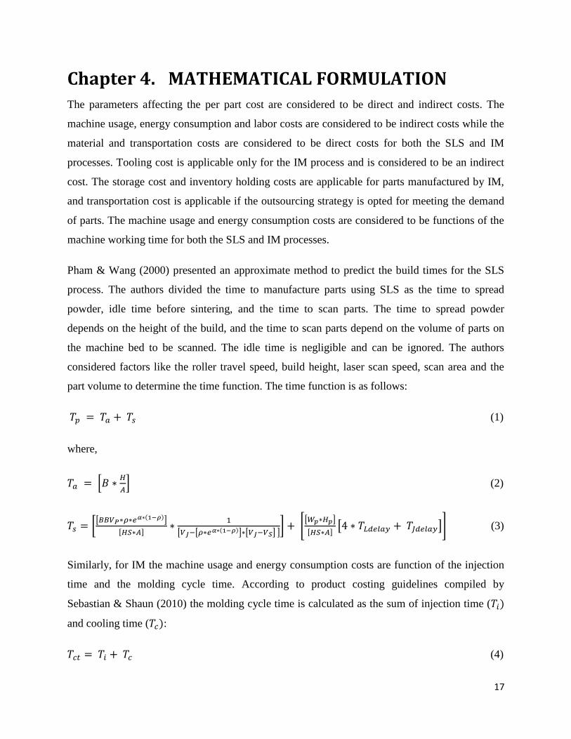
part volume to determine the time function. The time function is as follows:
(1)
where,
(2)
(3)
Similarly, for IM the machine usage and energy consumption costs are function of the injection
time and the molding cycle time. According to product costing guidelines compiled by
Sebastian & Shaun (2010) the molding cycle time is calculated as the sum of injection time (
and cooling time ( :
(4)

18
where,
(5)
The injection time is usually between 1 – 2 seconds. It should be noted that the values obtained
from the above equations are in seconds. Appropriate conversions are made according to
requirements in the cost functions and constraints in the following sections.
4.1 Cost Functions for SLS
The costs contributing to the per part cost for the SLS manufacturing process are as follows:
Machine usage cost
Energy consumption cost
Material cost
Labor cost
4.1.1 Machine usage cost
The machine usage cost is a function of the machine working time. It is calculated as the sum of
cost to add powder and cost to scan parts. The cost to add powder is calculated as a ratio of the
total time taken to add powder and the available machine time in the planning horizon multiplied
by the cost of machine. The cost to scan parts is calculated as a ratio of the total time taken to
scan parts and the available machine time in the planning horizon multiplied by the cost of the
machine. The machine working time to add powder ( and scan parts ( are taken from
equations (2) and (3).
(6)
(7)
4.1.2 Energy consumption cost
The energy consumption cost is also a function of the machine working time. The energy
consumption cost is calculated as the sum of cost to add powder and the cost to scan parts. The
cost to add powder is calculated as the product of time taken to add powder, power requirement
19
and cost of energy. The cost to scan parts is calculated as the product of the total time taken to
scan parts, power requirement, and cost of energy. The time taken to add powder ( and scan
parts ( are taken from equations (2) and (3).
(8)
(9)
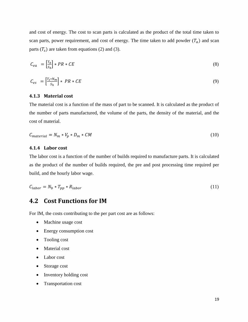
4.1.3 Material cost
The material cost is a function of the mass of part to be scanned. It is calculated as the product of
the number of parts manufactured, the volume of the parts, the density of the material, and the
cost of material.
(10)
4.1.4 Labor cost
The labor cost is a function of the number of builds required to manufacture parts. It is calculated
as the product of the number of builds required, the pre and post processing time required per
build, and the hourly labor wage.
(11)
4.2 Cost Functions for IM
For IM, the costs contributing to the per part cost are as follows:
Machine usage cost
Energy consumption cost
Tooling cost
Material cost
Labor cost
Storage cost
Inventory holding cost
Transportation cost

20
4.2.1 Machine usage cost
The machine usage cost is a function of the molding cycle time. It is calculated as a ratio of the
total molding cycle time required to manufacture parts and the available machine time in the
planning horizon multiplied by cost of machine. The molding cycle time is taken from equations
(4) and (5).
(12)
4.2.2 Energy consumption cost
The energy consumption cost is also a function of the molding cycle time. It is calculated as the
sum of cost to run machine and the cost of injection molding parts. The cost to run machine is
calculated as the product of total molding cycle time required to manufacture parts, power
requirement and cost of energy. The cost of injection molding parts is calculated as the product
of energy consumption of each molding cycle, number of parts produced and the cost of energy.
The molding cycle time is taken from equations (4) and (5).
(13)
4.2.3 Tooling cost
It is assumed for the cost analysis part of this research that the tool is available and the tooling
cost is calculated as the expected return on the tool cost for the planning period.
(14)
4.2.4 Material cost
The material cost is a function of the volume of part to be manufactured. It is calculated as the
product of the number of parts manufactured, the volume of the parts, the density of material,
and the cost of material. An additional 3% cost is considered as material wastage cost. The
material cost is calculated as follows:
(15)

21
4.2.5 Labor cost
The labor cost is calculated as the hourly labor wage multiplied by the sum of time taken to
change molds and the time taken to manufacture parts.
(16)
4.2.6 Storage cost
The storage cost is calculated as the product of number of parts stored, volume of parts and the
rate of storage.
(17)
4.2.7 Inventory holding cost
The inventory holding cost is calculated by adding the machine usage, energy consumption,
material, labor and storage costs for the number of parts stocked in inventory. This cost is
multiplied by the opportunity cost for holding inventory in each time period.
(18)
4.2.8 Transportation cost
The transportation cost is a function of the weight of the part to be shipped and the speed of
delivery. It is calculated as the product of number of parts shipped, volume of part, density of
material and the rate of transportation by mode of delivery selected.
(19)
A mixed integer linear programming mathematical model has been developed to determine the
cost of parts considering the system constraints. Consider an OEM who needs to determine
which supply chain strategy needs to be adopted to meet the demand of part p, p ϵ {1...P}. The
OEM has the option to manufacture by SLS on demand site dn, dn ϵ {1..DN} in time period t, t ϵ
{1..T} or ship parts stocked at a centrally located warehouse cl, cl ϵ {1...CL} manufactured by
IM. The OEM has the option to ship parts using the mode of shipment mps, mps ϵ {1...MPS}.
The notations, objective function and constraints in the model are explained below:

22
Sets
Parameters
Machine cost parameters
Variable cost parameters
SLS process parameters
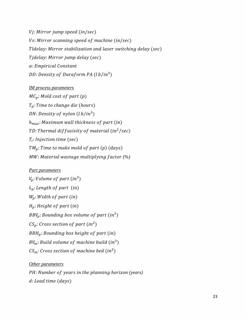
23
IM process parameters
(%)
Part parameters
Other parameters
(years)
24
Variables
Binary decision variables
Integer variables
Continuous variables
25
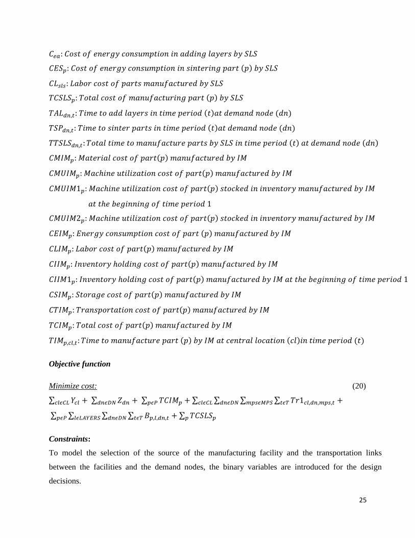
Objective function
Minimize cost: (20)
Constraints:
To model the selection of the source of the manufacturing facility and the transportation links
between the facilities and the demand nodes, the binary variables are introduced for the design
decisions.
26
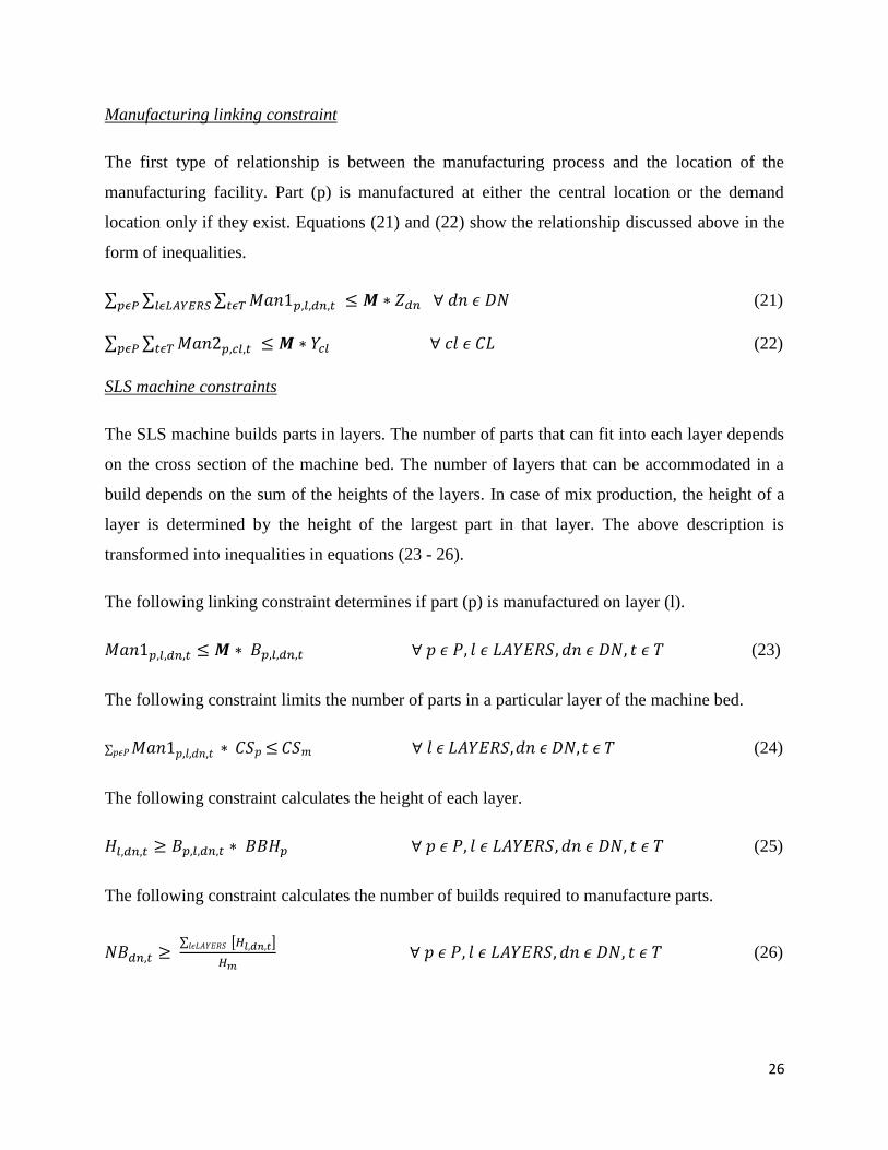
Manufacturing linking constraint
The first type of relationship is between the manufacturing process and the location of the
manufacturing facility. Part (p) is manufactured at either the central location or the demand
location only if they exist. Equations (21) and (22) show the relationship discussed above in the
form of inequalities.
(21)
(22)
SLS machine constraints
The SLS machine builds parts in layers. The number of parts that can fit into each layer depends
on the cross section of the machine bed. The number of layers that can be accommodated in a
build depends on the sum of the heights of the layers. In case of mix production, the height of a
layer is determined by the height of the largest part in that layer. The above description is
transformed into inequalities in equations (23 - 26).
The following linking constraint determines if part (p) is manufactured on layer (l).
(23)
The following constraint limits the number of parts in a particular layer of the machine bed.
(24)
The following constraint calculates the height of each layer.
(25)
The following constraint calculates the number of builds required to manufacture parts.
(26)
27
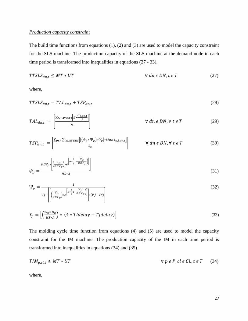
Production capacity constraint
The build time functions from equations (1), (2) and (3) are used to model the capacity constraint
for the SLS machine. The production capacity of the SLS machine at the demand node in each
time period is transformed into inequalities in equations (27 - 33).
(27)
where,
(28)
(29)
(30)
(31)
(32)
(33)
The molding cycle time function from equations (4) and (5) are used to model the capacity
constraint for the IM machine. The production capacity of the IM in each time period is
transformed into inequalities in equations (34) and (35).
(34)
where,
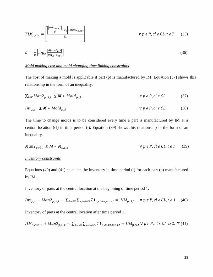
28
(35)
(36)
Mold making cost and mold changing time linking constraints
The cost of making a mold is applicable if part (p) is manufactured by IM. Equation (37) shows this
relationship in the form of an inequality.
(37)
(38)
The time to change molds is to be considered every time a part is manufactured by IM at a
central location (cl) in time period (t). Equation (39) shows this relationship in the form of an
inequality.
(39)
Inventory constraints
Equations (40) and (41) calculate the inventory in time period (t) for each part (p) manufactured
by IM.
Inventory of parts at the central location at the beginning of time period 1.
(40)
Inventory of parts at the central location after time period 1.
(41)

29
Lead time constraints
The total time to manufacture parts by SLS is the summation of the pre and post processing time
per build, time to add powder and time to scan parts. The total time should be within the desired
lead time at the demand node. Equation (42) expresses this relationship in the form of an
inequality.
(42)
The time to make the mold set up the mold, and manufacture and transport parts from the central
location to the demand node should be within the desired lead time. Equation (43) expresses this
relationship in the form of an inequality.
(43)
Transportation constraints
The cost and time of shipping parts from the central facility to demand node has to be considered
if demand is met from parts stocked at a central location. Equation (44) expresses this
relationship in the form of inequalities.
The binary variable takes the value 1 if transportation of parts takes place from central location
(cl) to demand node (dn).
(44)
Cost variables
Equation (45) calculates the machine utilization cost of parts stocked in inventory at the central
location at the beginning of time period 1.
(45)
30
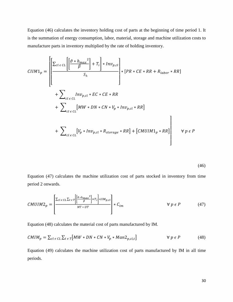
Equation (46) calculates the inventory holding cost of parts at the beginning of time period 1. It
is the summation of energy consumption, labor, material, storage and machine utilization costs to
manufacture parts in inventory multiplied by the rate of holding inventory.
(46)
Equation (47) calculates the machine utilization cost of parts stocked in inventory from time
period 2 onwards.
(47)
Equation (48) calculates the material cost of parts manufactured by IM.
(48)
Equation (49) calculates the machine utilization cost of parts manufactured by IM in all time
periods.

31
(49)
Equation (50) calculates the energy consumption cost of parts manufactured by IM in all time
periods.
(50)
Equation (51) calculates the labor cost of parts manufactured by IM in all time periods.
(51)
Equation (52) calculates the cost of storing parts in inventory for all time periods as follows:
(52)
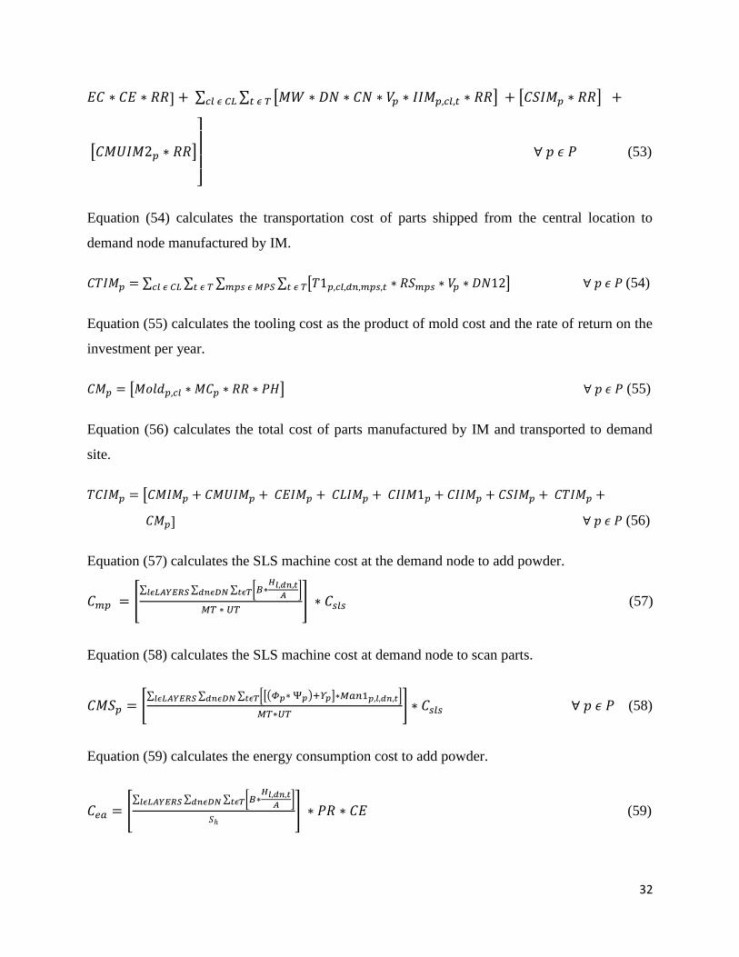
Equation (53) calculates the inventory holding cost of parts stocked in inventory as the
summation of energy consumption, labor, material, storage and machine utilization costs
multiplied by the rate of return on investment.
32
(53)
Equation (54) calculates the transportation cost of parts shipped from the central location to
demand node manufactured by IM.
(54)
Equation (55) calculates the tooling cost as the product of mold cost and the rate of return on the
investment per year.
(55)
Equation (56) calculates the total cost of parts manufactured by IM and transported to demand
site.
(56)
Equation (57) calculates the SLS machine cost at the demand node to add powder.
(57)
Equation (58) calculates the SLS machine cost at demand node to scan parts.
(58)
Equation (59) calculates the energy consumption cost to add powder.
(59)
33
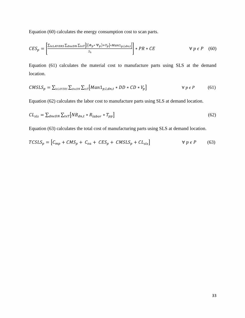
Equation (60) calculates the energy consumption cost to scan parts.
(60)
Equation (61) calculates the material cost to manufacture parts using SLS at the demand
location.
(61)
Equation (62) calculates the labor cost to manufacture parts using SLS at demand location.
(62)
Equation (63) calculates the total cost of manufacturing parts using SLS at demand location.
(63)

34
Chapter 5. RESEARCH METHODOLOGY
A set of parameters values were to be selected as input data to the mathematical model presented
in Chapter 4. These parameters are listed below:
1. Type of part
2. Process capability and machine specifications (SLS and IM)
3. Demand quantity
4. Cost and time parameters
The selection of values for the above mentioned parameters is elaborated in the following sub
sections.
5.1 Type of Part
The complexity and size of part to be manufactured is an important factor which influences the
unit cost of parts manufactured by IM. The IM process is typically used to manufacture thin
walled cylindrical, cubical and complex geometries, while the SLS process can manufacture
thicker cylindrical, cubical and complex geometries too. SLS can be used to manufacture parts of
any complexity without the need of additional processing to achieve the required geometry. For
this research, six representative parts differing in dimension, shape and complexity have been
selected.
Figure 7 : Bracket (GRABCAD, 2013a)

35
Figure 8 : Gear (GRABCAD, 2013b)
Figure 9 : Horn (GRABCAD, 2013c)
Figure 10 : Impeller (GRABCAD, 2013d)

36
Figure 11 : Plastic Impeller (GRABCAD, 2013e)
Figure 12 : Spur gear (GRABCAD, 2013f)
The following table summarizes the assumptions of the part complexities for estimating the tool
cost for IM:
Table 3 : Part Complexity
Maximum Wall Thickness (in) 0.2
Tolerance (in) Moderate Precision ( 0.01)
Surface Roughness (µ in) Normal Polish (Ra 16)
Complexity Complex
For the SLS process, the smallest box that is able to contain the part is referred to as the
‘bounding box’. In this research, the bounding box volume for each part is calculated by adding
0.5” on each dimension. The smallest dimension is assumed to be the height of the part. The
table below summarizes the actual and bounding box dimensions of the parts under
consideration.
37
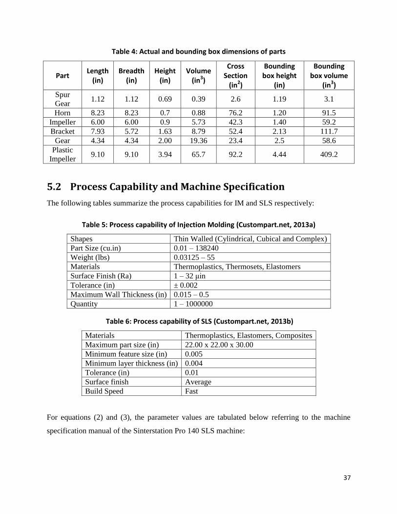
Table 4: Actual and bounding box dimensions of parts
Part Length
(in) Breadth
(in) Height
(in) Volume
(in3)
Cross Section
(in2)
Bounding box height
(in)
Bounding box volume
(in3) Spur
Gear 1.12 1.12 0.69 0.39 2.6 1.19 3.1
Horn 8.23 8.23 0.7 0.88 76.2 1.20 91.5
Impeller 6.00 6.00 0.9 5.73 42.3 1.40 59.2
Bracket 7.93 5.72 1.63 8.79 52.4 2.13 111.7
Gear 4.34 4.34 2.00 19.36 23.4 2.5 58.6
Plastic
Impeller 9.10 9.10 3.94 65.7 92.2 4.44 409.2
5.2 Process Capability and Machine Specification
The following tables summarize the process capabilities for IM and SLS respectively:
Table 5: Process capability of Injection Molding (Custompart.net, 2013a)
Shapes Thin Walled (Cylindrical, Cubical and Complex)
Part Size (cu.in) 0.01 – 138240
Weight (lbs) 0.03125 – 55
Materials Thermoplastics, Thermosets, Elastomers
Surface Finish (Ra) 1 – 32 μin
Tolerance (in) ± 0.002
Maximum Wall Thickness (in) 0.015 – 0.5
Quantity 1 – 1000000
Table 6: Process capability of SLS (Custompart.net, 2013b)
Materials Thermoplastics, Elastomers, Composites
Maximum part size (in) 22.00 x 22.00 x 30.00
Minimum feature size (in) 0.005
Minimum layer thickness (in) 0.004
Tolerance (in) 0.01
Surface finish Average
Build Speed Fast
For equations (2) and (3), the parameter values are tabulated below referring to the machine
specification manual of the Sinterstation Pro 140 SLS machine:

38
Table 7: Sinterstation Pro 140 machine specifications (Systems, 2007)
Parameter Value
Time spent spreading a layer of powder (sec) 22.5
Thickness of powder layer (in) 0.004
Laser scan spacing in the Y direction (in) 0.006
Mirror jump speed (in/sec) 203.2
Mirror scanning speed (in/sec) 240
Mirror stabilization and laser switch delay (sec) 0.0037
Mirror jump delay (sec) 0.002
Roller travel speed (in/sec) 5
5.3 Demand Quantity
The manufacturing process and the mode of transportation to be selected in a ‘just in time’
environment depend on the desired lead time and the demand quantity. For this research, a lead
time of 7 days is considered. Three levels of demand quantities are considered for this research
such as low, medium and high demand. As the tool cost contributes significantly to the unit cost
of part manufactured by IM, the demand quantities are calculated as the ratio of opportunity cost
of investment in tool per year to the unit cost of part as a percentage of the opportunity cost of
investment in tool per year. The rate of return on the investment is assumed to be 30% per
annum. The table below lists the unit cost of a part considered as a percentage of the opportunity
cost of investment in tool per year for the three levels of demand quantities:
Table 8: Demand levels
Demand
Level
Percentage of opportunity cost of investment in tool per year to
calculate unit cost of part
No of
parts
Low 1% 100
Medium 0.1% 1000
High 0.01% 10000
5.4 Cost and Time Parameters
5.4.1 Material cost
The material to manufacture parts for this study is considered to be nylon. The material cost for
nylon SLS powder is considerably higher than the cost of nylon IM pellets. The material
specifications used in the time and cost functions for IM and SLS are tabulated below:

39
Table 9: Material cost and specification (Corporation, 2010) (Custompart.net, 2013a)
Material Density
(lb/in3)
Thermal
diffusivity
(in2/sec)
Material
cost
($/lb)
Part ejection
temperature
(°C)
Mold
temperature
(°C)
Polymer
injection
temperature
(°C)
Nylon
(IM) 0.025 0.000144 3.5 129 91 291
Duraform
PA
(SLS)
0.036 - 64.2 - - -
5.4.2 Machine cost
The machine usage cost for both IM and SLS is calculated as the ratio of total machine
utilization time to the total available machine time in the machine depreciation period. It is
assumed that the machine utilization rate for both the processes is 70%. The machine cost for IM
is estimated to be approximately $300,000 for a reasonably high tonnage press of 200 tons. For
this research, the Sinterstation Pro 140 was selected with an assumed cost of $300,000. The table
below gives the cost of different SLS machines along with their build capacity and printing
speeds:
Table 10: Machine cost and specification (Corporation, 2010)
Machine Approximate
Cost ($)
Cross section of
machine bed (in2)
Maximum machine build
volume (in3)
Sinterstation HiQ 245,888 168 3024
Sinterstation Pro
140 391,916 195 3500
Sinterstation Pro
230 484,447 471 13891
5.4.3 Tool cost
The tool cost is the fixed cost associated with the IM process whereas no tooling is required for
the SLS process. The tool cost for the parts under consideration is tabulated below:

40
Table 11: Tool Cost (Custompart.net, 2013a)
Part Tool cost ($)
Spur Gear 14,600
Horn 28,900
Impeller 30,700
Bracket 29,300
Gear 32,300
Plastic Impeller 39,700
5.4.4 Energy, labor and inventory costs
According to the Sinterstation Pro 140 specifications, the power requirement for the Sinterstation
Pro 140 system is 22 kW. The power requirement for a 200 ton injection molding machine is
estimated to be 15 kW, and the energy consumption for a molding cycle is estimated to be 0.04
kWh. The cost of energy consumption was chosen referring to the ‘U.S Energy Information
Administration (EIA)’ website. The hourly labor wage was chosen referring to the ‘United States
Department of Labor’ website. The rate of return on investment was assumed to be 30% per
annum. The following table summarizes these cost parameters:
Table 12: Rate of Energy, Labor and Storage Parameter Value
Rate of energy consumption ($/kW-hour) 0.07
Labor wage ($/hour) 18
Rate of storing inventory ($/cu.in/week) 0.0009
Rate of return on capital invested 30%
5.4.5 Transportation
The transportation cost is a function of the weight of part to be shipped and the service level
desired. In the following table, an assumption for the shipping cost per pound is summarized
depending on the service level desired.
Table 13: Rate of shipping
Service Cost ($/lb)
1 Day 5
3 Days 10
5 Days 15

41
5.4.6 Time
The machine depreciation period was assumed to be 8 years. The pre and post processing time
per build for the SLS process and the time to change die was assumed to be 3 hours.

42
Chapter 6. EXPERIMENTAL RESULTS & ANALYSIS
As proposed in Section 1.3, one of the objectives of this thesis is to find the significant part
parameters affecting the unit supply chain cost of parts manufactured by SLS.
6.1 Preliminary Experimental Results
A set of preliminary experiments were run to compare the supply chain costs of the two
strategies under consideration. Table 14 shows estimated mold costs for each of the
demonstration parts. The third column then lists the opportunity cost associated with investing
money in a mold rather than another investment with an assumed return of 30%. The final three
columns then show this opportunity cost divided by the number of parts under the low (100),
medium (1000), and high (10,000) replacement part demand scenarios. Note that these demand
levels pertain specifically to spare/replacement parts rather than production of original run parts.
Table 14: Unit mold cost of parts
Part
Mold
Cost
($)
Opportunity cost
of investment in
tool per year
($)
Opportunity
cost per part
for low
demand
($/part)
Opportunity
cost per part
for medium
demand
($/part)
Opportunity
cost per part
for high
demand
($/part)
Spur
Gear 14,600 4,380 44 4 0.04
Horn 28,900 8,670 87 9 0.09
Impeller 30,700 9,210 92 9 0.09
Bracket 29,300 8,790 88 9 0.09
Gear 32,300 9,690 97 10 0.10
Plastic
Impeller 39,700 11,910 119 12 0.12
Experiments were run for a planning horizon of 50 time periods for the three demand levels. An
average order quantity of 2, 20 and 200 parts per time period for the low, medium and high
demand levels was assumed. The unit supply chain cost of parts under consideration for the three
demand levels using the supply chain strategy to manufacture by IM and stock to meet future
demands is tabulated below:
43
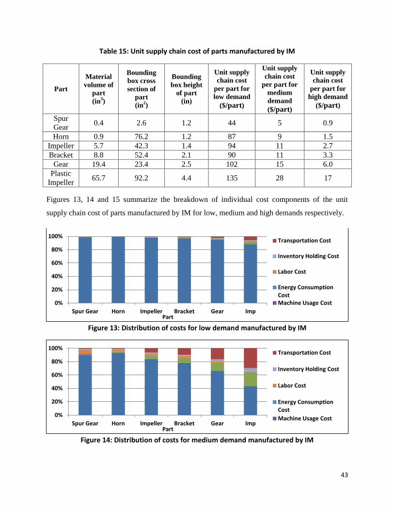
Table 15: Unit supply chain cost of parts manufactured by IM
Part
Material
volume of
part
(in3)
Bounding
box cross
section of
part
(in2)
Bounding
box height
of part
(in)
Unit supply
chain cost
per part for
low demand
($/part)
Unit supply
chain cost
per part for
medium
demand
($/part)
Unit supply
chain cost
per part for
high demand
($/part)
Spur
Gear 0.4 2.6 1.2 44 5 0.9
Horn 0.9 76.2 1.2 87 9 1.5
Impeller 5.7 42.3 1.4 94 11 2.7
Bracket 8.8 52.4 2.1 90 11 3.3
Gear 19.4 23.4 2.5 102 15 6.0
Plastic
Impeller 65.7 92.2 4.4 135 28 17
Figures 13, 14 and 15 summarize the breakdown of individual cost components of the unit
supply chain cost of parts manufactured by IM for low, medium and high demands respectively.
Figure 13: Distribution of costs for low demand manufactured by IM
Figure 14: Distribution of costs for medium demand manufactured by IM
0%
20%
40%
60%
80%
100%
Spur Gear Horn Impeller Bracket Gear Imp Part
Transportation Cost
Inventory Holding Cost
Labor Cost
Energy Consumption Cost Machine Usage Cost
0%
20%
40%
60%
80%
100%
Spur Gear Horn Impeller Bracket Gear Imp Part
Transportation Cost
Inventory Holding Cost
Labor Cost
Energy Consumption Cost
Machine Usage Cost
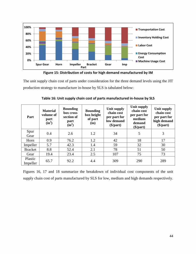
44
Figure 15: Distribution of costs for high demand manufactured by IM
The unit supply chain cost of parts under consideration for the three demand levels using the JIT
production strategy to manufacture in-house by SLS is tabulated below:
Table 16: Unit supply chain cost of parts manufactured in-house by SLS
Part
Material
volume of
part
(in3)
Bounding
box cross
section of
part
(in2)
Bounding
box height
of part
(in)
Unit supply
chain cost
per part for
low demand
($/part)
Unit supply
chain cost
per part for
medium
demand
($/part)
Unit supply
chain cost
per part for
high demand
($/part)
Spur
Gear 0.4 2.6 1.2 34 5 3
Horn 0.9 76.2 1.2 42 18 17
Impeller 5.7 42.3 1.4 59 32 30
Bracket 8.8 52.4 2.1 78 51 50
Gear 19.4 23.4 2.5 107 75 73
Plastic
Impeller 65.7 92.2 4.4 309 290 289
Figures 16, 17 and 18 summarize the breakdown of individual cost components of the unit
supply chain cost of parts manufactured by SLS for low, medium and high demands respectively.
0%
20%
40%
60%
80%
100%
Spur Gear Horn Impeller Bracket Gear Imp Part
Transportation Cost
Inventory Holding Cost
Labor Cost
Energy Consumption Cost
Machine Usage Cost

45
Figure 16: Distribution of costs for low demand manufactured by SLS
Figure 17: Distribution of costs for medium demand manufactured by SLS
Figure 18: Distribution of costs for high demand manufactured by SLS
0%
20%
40%
60%
80%
100%
Spur Gear Horn Impeller Bracket Gear Imp
Part
Labor Cost
Energy Consumption Cost
Machine Usage Cost
Material Cost
0%
20%
40%
60%
80%
100%
Spur Gear Horn Impeller Bracket Gear Imp
Part
Labor Cost
Energy Consumption Cost
Machine Usage Cost
Material Cost
0%
20%
40%
60%
80%
100%
Spur Gear Horn Impeller Bracket Gear Imp
Part
Labor Cost
Energy Consumption Cost
Machine Usage Cost
Material Cost
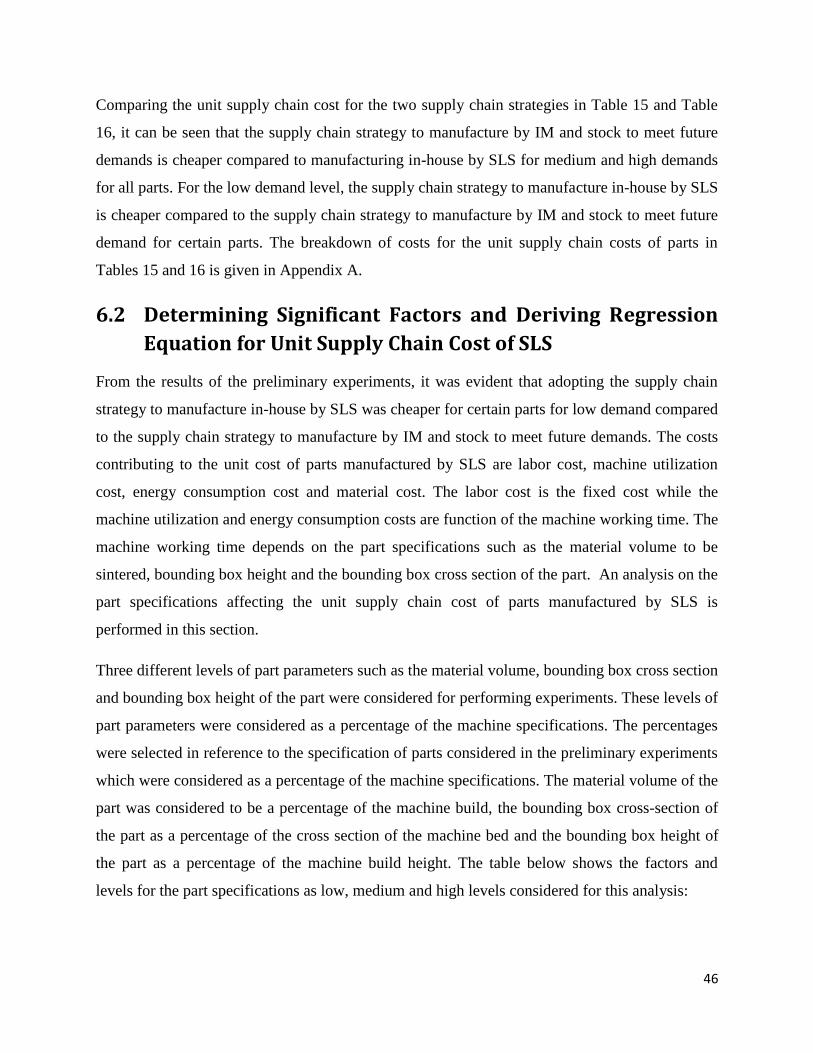
46
Comparing the unit supply chain cost for the two supply chain strategies in Table 15 and Table
16, it can be seen that the supply chain strategy to manufacture by IM and stock to meet future
demands is cheaper compared to manufacturing in-house by SLS for medium and high demands
for all parts. For the low demand level, the supply chain strategy to manufacture in-house by SLS
is cheaper compared to the supply chain strategy to manufacture by IM and stock to meet future
demand for certain parts. The breakdown of costs for the unit supply chain costs of parts in
Tables 15 and 16 is given in Appendix A.
6.2 Determining Significant Factors and Deriving Regression
Equation for Unit Supply Chain Cost of SLS
From the results of the preliminary experiments, it was evident that adopting the supply chain
strategy to manufacture in-house by SLS was cheaper for certain parts for low demand compared
to the supply chain strategy to manufacture by IM and stock to meet future demands. The costs
contributing to the unit cost of parts manufactured by SLS are labor cost, machine utilization
cost, energy consumption cost and material cost. The labor cost is the fixed cost while the
machine utilization and energy consumption costs are function of the machine working time. The
machine working time depends on the part specifications such as the material volume to be
sintered, bounding box height and the bounding box cross section of the part. An analysis on the
part specifications affecting the unit supply chain cost of parts manufactured by SLS is
performed in this section.
Three different levels of part parameters such as the material volume, bounding box cross section
and bounding box height of the part were considered for performing experiments. These levels of
part parameters were considered as a percentage of the machine specifications. The percentages
were selected in reference to the specification of parts considered in the preliminary experiments
which were considered as a percentage of the machine specifications. The material volume of the
part was considered to be a percentage of the machine build, the bounding box cross-section of
the part as a percentage of the cross section of the machine bed and the bounding box height of
the part as a percentage of the machine build height. The table below shows the factors and
levels for the part specifications as low, medium and high levels considered for this analysis:

47
Table 17: Levels of part specifications with respect to machine specifications
Factor Low level Medium level High level
A (Material Volume) 0.5% of machine
build volume
1% of machine build
volume
1.5% of machine
build volume
B (Bounding box
height)
5% of machine build
height
10% of machine build
height
15% of machine build
height
C (Bounding box
cross section)
25% of machine bed
cross section
50% of machine bed
cross section
75% of machine bed
cross section
The results of the experiments obtained from running the mathematical model for the
experimental setup in Table 17 are given in Appendix B. Minitab 17 statistical software was used
to generate a general full factorial design with three factors and three levels for each factor, for a
total of 27 runs. The predictor variables were Factor A (Material Volume), Factor B (Bounding
Box Height of Part) and Factor C (Bounding Box Cross Section of Part). A regression model was
run with Factor A (Material Volume), Factor B (Bounding Box Height of Part), Factor C
(Bounding Box Cross Section of Part), the interaction of factors A & B (Material Volume &
Bounding Box Height of Part), the interaction of factors B & C (Bounding Box Height of Part &
Bounding Box Cross Section of Part), the interaction of factors A & C (Material Volume &
Bounding Box Cross Section of Part) and interaction of factors A, B & C (Material Volume,
Bounding Box Cross Height of Part & Bounding Box Cross Section of Part). The unit supply
chain cost of part for the supply chain strategy to manufacture in-house by SLS was the response
variable. The ANOVA for the model is provided in Figure 19.
Figure 19: Analysis of variance for the full regression model
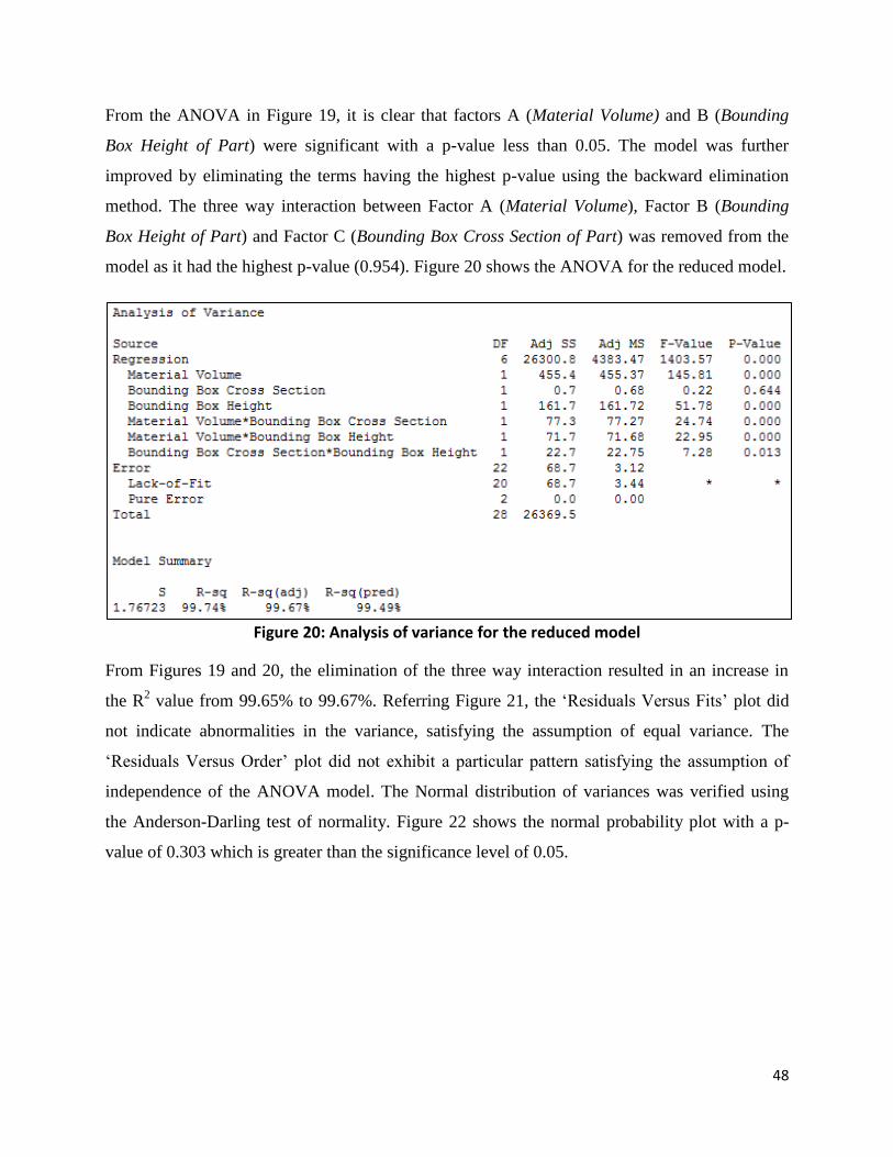
48
From the ANOVA in Figure 19, it is clear that factors A (Material Volume) and B (Bounding
Box Height of Part) were significant with a p-value less than 0.05. The model was further
improved by eliminating the terms having the highest p-value using the backward elimination
method. The three way interaction between Factor A (Material Volume), Factor B (Bounding
Box Height of Part) and Factor C (Bounding Box Cross Section of Part) was removed from the
model as it had the highest p-value (0.954). Figure 20 shows the ANOVA for the reduced model.
Figure 20: Analysis of variance for the reduced model
From Figures 19 and 20, the elimination of the three way interaction resulted in an increase in
the R2 value from 99.65% to 99.67%. Referring Figure 21, the ‘Residuals Versus Fits’ plot did
not indicate abnormalities in the variance, satisfying the assumption of equal variance. The
‘Residuals Versus Order’ plot did not exhibit a particular pattern satisfying the assumption of
independence of the ANOVA model. The Normal distribution of variances was verified using
the Anderson-Darling test of normality. Figure 22 shows the normal probability plot with a p-
value of 0.303 which is greater than the significance level of 0.05.
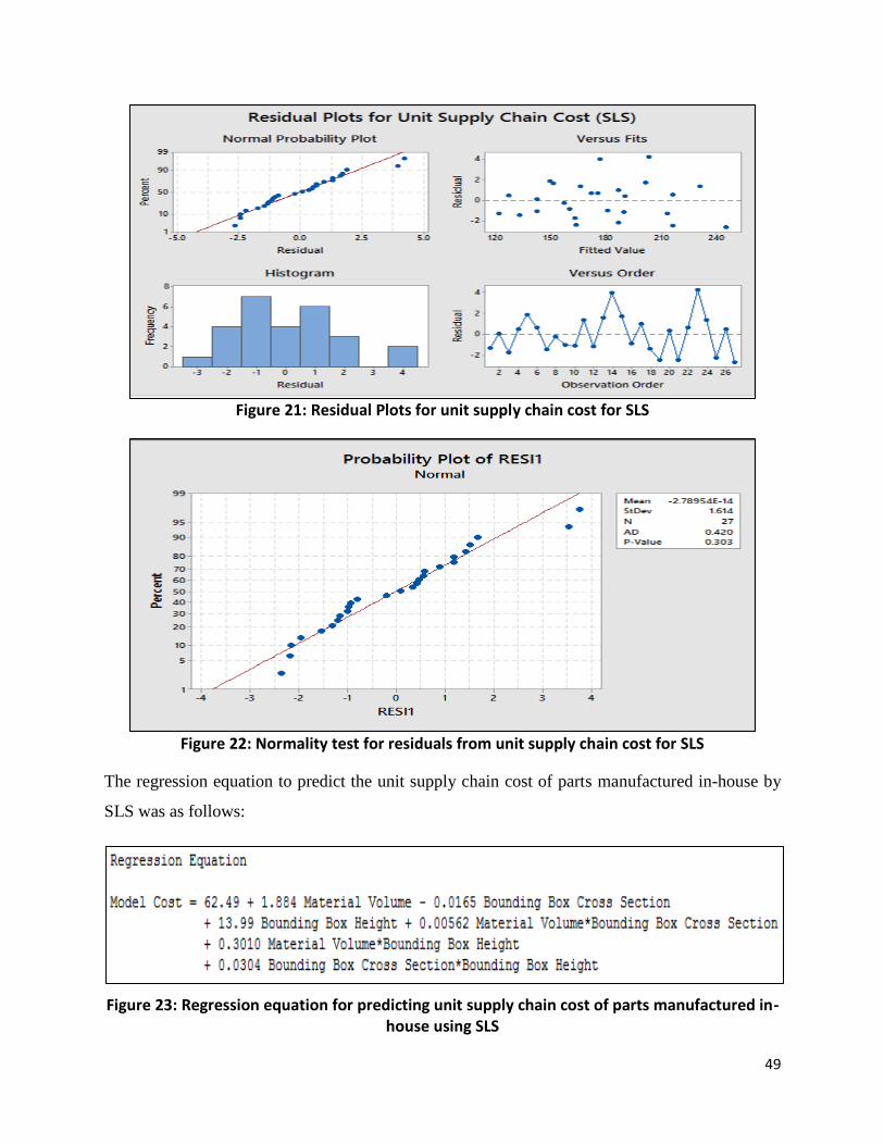
49
Figure 21: Residual Plots for unit supply chain cost for SLS
Figure 22: Normality test for residuals from unit supply chain cost for SLS
The regression equation to predict the unit supply chain cost of parts manufactured in-house by
SLS was as follows:
Figure 23: Regression equation for predicting unit supply chain cost of parts manufactured in-house using SLS
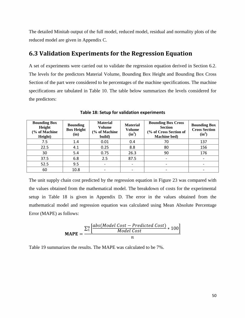
50
The detailed Minitab output of the full model, reduced model, residual and normality plots of the
reduced model are given in Appendix C.
6.3 Validation Experiments for the Regression Equation
A set of experiments were carried out to validate the regression equation derived in Section 6.2.
The levels for the predictors Material Volume, Bounding Box Height and Bounding Box Cross
Section of the part were considered to be percentages of the machine specifications. The machine
specifications are tabulated in Table 10. The table below summarizes the levels considered for
the predictors:
Table 18: Setup for validation experiments
Bounding Box
Height
(% of Machine
Height)
Bounding
Box Height
(in)
Material
Volume
(% of Machine
build)
Material
Volume
(in3)
Bounding Box Cross
Section
(% of Cross Section of
Machine bed)
Bounding Box
Cross Section
(in2)
7.5 1.4 0.01 0.4 70 137 22.5 4.1 0.25 8.8 80 156 30 5.4 0.75 26.3 90 176
37.5 6.8 2.5 87.5 - - 52.5 9.5 - - - - 60 10.8 - - - -
The unit supply chain cost predicted by the regression equation in Figure 23 was compared with
the values obtained from the mathematical model. The breakdown of costs for the experimental
setup in Table 18 is given in Appendix D. The error in the values obtained from the
mathematical model and regression equation was calculated using Mean Absolute Percentage
Error (MAPE) as follows:
Table 19 summarizes the results. The MAPE was calculated to be 7%.
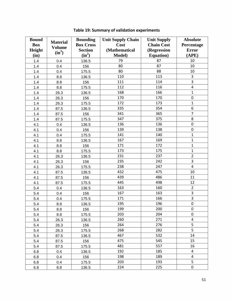
51
Table 19: Summary of validation experiments
Bound
Box
Height
(in)
Material
Volume
(in3)
Bounding
Box Cross
Section
(in2)
Unit Supply Chain
Cost
(Mathematical
Model)
Unit Supply
Chain Cost
(Regression
Equation)
Absolute
Percentage
Error
(APE)
1.4 0.4 136.5 79 87 10
1.4 0.4 156 80 87 10
1.4 0.4 175.5 80 88 10
1.4 8.8 136.5 110 113 3
1.4 8.8 156 111 114 3
1.4 8.8 175.5 112 116 4
1.4 26.3 136.5 168 166 1
1.4 26.3 156 170 170 0
1.4 26.3 175.5 172 173 1
1.4 87.5 136.5 335 354 6
1.4 87.5 156 341 365 7
1.4 87.5 175.5 347 375 8
4.1 0.4 136.5 136 136 0
4.1 0.4 156 139 138 0
4.1 0.4 175.5 141 140 1
4.1 8.8 136.5 167 169 1
4.1 8.8 156 171 172 1
4.1 8.8 175.5 173 175 1
4.1 26.3 136.5 231 237 2
4.1 26.3 156 235 242 3
4.1 26.3 175.5 238 247 4
4.1 87.5 136.5 432 475 10
4.1 87.5 156 439 486 11
4.1 87.5 175.5 445 498 12
5.4 0.4 136.5 163 160 2
5.4 0.4 156 167 163 3
5.4 0.4 175.5 171 166 3
5.4 8.8 136.5 195 196 0
5.4 8.8 156 199 200 0
5.4 8.8 175.5 203 204 0
5.4 26.3 136.5 260 271 4
5.4 26.3 156 264 276 5
5.4 26.3 175.5 268 282 5
5.4 87.5 136.5 467 532 14
5.4 87.5 156 475 545 15
5.4 87.5 175.5 481 557 16
6.8 0.4 136.5 192 185 4
6.8 0.4 156 198 189 4
6.8 0.4 175.5 203 193 5
6.8 8.8 136.5 224 225 0
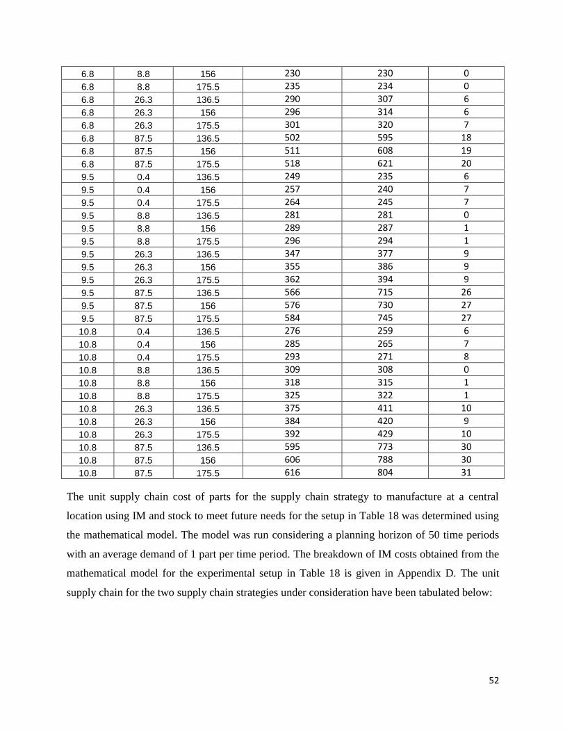
52
6.8 8.8 156 230 230 0
6.8 8.8 175.5 235 234 0
6.8 26.3 136.5 290 307 6
6.8 26.3 156 296 314 6
6.8 26.3 175.5 301 320 7
6.8 87.5 136.5 502 595 18
6.8 87.5 156 511 608 19
6.8 87.5 175.5 518 621 20
9.5 0.4 136.5 249 235 6
9.5 0.4 156 257 240 7
9.5 0.4 175.5 264 245 7
9.5 8.8 136.5 281 281 0
9.5 8.8 156 289 287 1
9.5 8.8 175.5 296 294 1
9.5 26.3 136.5 347 377 9
9.5 26.3 156 355 386 9
9.5 26.3 175.5 362 394 9
9.5 87.5 136.5 566 715 26
9.5 87.5 156 576 730 27
9.5 87.5 175.5 584 745 27
10.8 0.4 136.5 276 259 6
10.8 0.4 156 285 265 7
10.8 0.4 175.5 293 271 8
10.8 8.8 136.5 309 308 0
10.8 8.8 156 318 315 1
10.8 8.8 175.5 325 322 1
10.8 26.3 136.5 375 411 10
10.8 26.3 156 384 420 9
10.8 26.3 175.5 392 429 10
10.8 87.5 136.5 595 773 30
10.8 87.5 156 606 788 30
10.8 87.5 175.5 616 804 31
The unit supply chain cost of parts for the supply chain strategy to manufacture at a central
location using IM and stock to meet future needs for the setup in Table 18 was determined using
the mathematical model. The model was run considering a planning horizon of 50 time periods
with an average demand of 1 part per time period. The breakdown of IM costs obtained from the
mathematical model for the experimental setup in Table 18 is given in Appendix D. The unit
supply chain for the two supply chain strategies under consideration have been tabulated below:
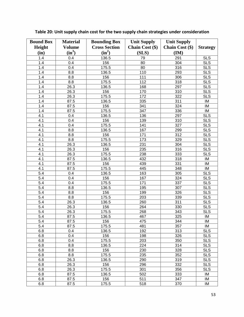
53
Table 20: Unit supply chain cost for the two supply chain strategies under consideration
Bound Box
Height
(in)
Material
Volume
(in3)
Bounding Box
Cross Section
(in2)
Unit Supply
Chain Cost ($)
(SLS)
Unit Supply
Chain Cost ($)
(IM)
Strategy
1.4 0.4 136.5 79 291 SLS
1.4 0.4 156 80 304 SLS
1.4 0.4 175.5 80 316 SLS
1.4 8.8 136.5 110 293 SLS
1.4 8.8 156 111 306 SLS
1.4 8.8 175.5 112 318 SLS
1.4 26.3 136.5 168 297 SLS
1.4 26.3 156 170 310 SLS
1.4 26.3 175.5 172 322 SLS
1.4 87.5 136.5 335 311 IM
1.4 87.5 156 341 324 IM
1.4 87.5 175.5 347 336 IM
4.1 0.4 136.5 136 297 SLS
4.1 0.4 156 139 310 SLS
4.1 0.4 175.5 141 327 SLS
4.1 8.8 136.5 167 299 SLS
4.1 8.8 156 171 312 SLS
4.1 8.8 175.5 173 329 SLS
4.1 26.3 136.5 231 304 SLS
4.1 26.3 156 235 316 SLS
4.1 26.3 175.5 238 333 SLS
4.1 87.5 136.5 432 318 IM
4.1 87.5 156 439 331 IM
4.1 87.5 175.5 445 348 IM
5.4 0.4 136.5 163 305 SLS
5.4 0.4 156 167 324 SLS
5.4 0.4 175.5 171 337 SLS
5.4 8.8 136.5 195 307 SLS
5.4 8.8 156 199 326 SLS
5.4 8.8 175.5 203 339 SLS
5.4 26.3 136.5 260 311 SLS
5.4 26.3 156 264 330 SLS
5.4 26.3 175.5 268 343 SLS
5.4 87.5 136.5 467 325 IM
5.4 87.5 156 475 344 IM
5.4 87.5 175.5 481 357 IM
6.8 0.4 136.5 192 313 SLS
6.8 0.4 156 198 326 SLS
6.8 0.4 175.5 203 350 SLS
6.8 8.8 136.5 224 314 SLS
6.8 8.8 156 230 328 SLS
6.8 8.8 175.5 235 352 SLS
6.8 26.3 136.5 290 319 SLS
6.8 26.3 156 296 332 SLS
6.8 26.3 175.5 301 356 SLS
6.8 87.5 136.5 502 333 IM
6.8 87.5 156 511 347 IM
6.8 87.5 175.5 518 370 IM
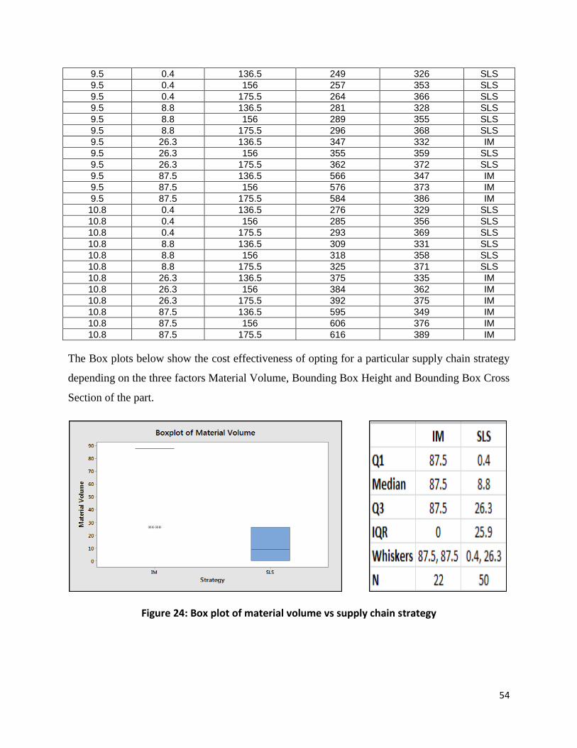
54
9.5 0.4 136.5 249 326 SLS
9.5 0.4 156 257 353 SLS
9.5 0.4 175.5 264 366 SLS
9.5 8.8 136.5 281 328 SLS
9.5 8.8 156 289 355 SLS
9.5 8.8 175.5 296 368 SLS
9.5 26.3 136.5 347 332 IM
9.5 26.3 156 355 359 SLS
9.5 26.3 175.5 362 372 SLS
9.5 87.5 136.5 566 347 IM
9.5 87.5 156 576 373 IM
9.5 87.5 175.5 584 386 IM
10.8 0.4 136.5 276 329 SLS
10.8 0.4 156 285 356 SLS
10.8 0.4 175.5 293 369 SLS
10.8 8.8 136.5 309 331 SLS
10.8 8.8 156 318 358 SLS
10.8 8.8 175.5 325 371 SLS
10.8 26.3 136.5 375 335 IM
10.8 26.3 156 384 362 IM
10.8 26.3 175.5 392 375 IM
10.8 87.5 136.5 595 349 IM
10.8 87.5 156 606 376 IM
10.8 87.5 175.5 616 389 IM
The Box plots below show the cost effectiveness of opting for a particular supply chain strategy
depending on the three factors Material Volume, Bounding Box Height and Bounding Box Cross
Section of the part.
Figure 24: Box plot of material volume vs supply chain strategy

55
Figure 25: Box plot of bounding box height vs supply chain strategy
Figure 26: Box plot of bounding box cross section vs supply chain strategy
From the Box plots in Figures 24, 25 and 26, it is evident that the supply chain strategy to
manufacture on demand site using SLS is cheaper compared to the supply chain strategy to
manufacture by IM except for parts with the highest level of material volume 87.5 in3 (2.5% of
the machine build). The Bounding Box Height and Bounding Box Cross Section of part do not
favor a particular supply chain strategy.
The effect of tool cost for IM on the supply chain strategy was carried out by varying the cost of
the tool by 25%. The Box plot in Figure 27 shows that if the tool cost is reduced by 25%, then
IM becomes the more economical supply chain strategy for parts with high material volume.
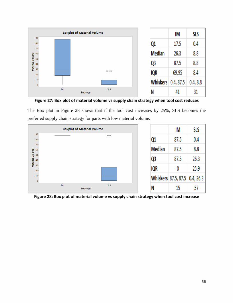
56
Figure 27: Box plot of material volume vs supply chain strategy when tool cost reduces
The Box plot in Figure 28 shows that if the tool cost increases by 25%, SLS becomes the
preferred supply chain strategy for parts with low material volume.
Figure 28: Box plot of material volume vs supply chain strategy when tool cost increase
57
Chapter 7. CONCLUSIONS & FUTURE WORK
A detailed model showing the conditions under which low part demands are economically
satisfied using on-demand SLS manufacturing rather than conventional injection molding was
developed. The part specification contributing significantly to the supply chain cost of parts
manufactured by SLS were determined using regression analysis. Material Volume, Part
Bounding Box Height, and the two way interactions between Material Volume, Bounding Box
Height, and Part Bounding Box Cross Section proved to be the significant factors. A regression
equation to predict the unit supply chain cost of parts manufactured in-house was derived and
validated with a MAPE of 7%. From the box plot in Figure 24, it can be said that parts having
low material volume relative to the machine build are cheaper to produce via SLS than
manufacturing by IM, particularly when part quantities are low. The tool cost for IM plays a
significant role in the decision making process and is illustrated in Figures 27 and 28.
In this research, the cost of molds was referenced from an online source (Custompart.net). An
equation to predict the unit supply chain cost of a part manufactured by IM can be derived
considering part specifications and complexities. An equation predicting the cheaper supply
chain strategy considering supply chain parameters such as lead time, part specifications and
demand quantity can be an interesting area of study. The mathematical model developed in this
research to estimate the economical supply chain strategy with respect to part parameters can be
used to optimize the supply chain as a future work.
58
REFERENCES
3D Printing Industry, Explore the Many Uses of FDM | Stratasys. (2014). Retrieved from http://www.stratasys.com/industries
Additive Fabrication Transforms Dental Labs. (2008, 2008-06-11). Retrieved from http://www.rapidtoday.com/dental.html
Atzeni, E., Iuliano, L., Minetola, P., & Salmi, A. (2010). Redesign and cost estimation of rapid manufactured plastic parts. Rapid Prototyping Journal, 16(5), 308-317.
Berman, B. (2012). 3-D printing: The new industrial revolution. Business horizons, 55(2), 155-162. Chandra, A., Watson, J., Rowson, J., Holland, J., Harris, R., & Williams, D. (2005). Application of rapid
manufacturing techniques in support of maxillofacial treatment: evidence of the requirements of clinical applications. Proceedings of the Institution of Mechanical Engineers, Part B: Journal of Engineering Manufacture, 219(6), 469-475.
Christopher, M. (2000). The agile supply chain: competing in volatile markets. Industrial marketing management, 29(1), 37-44.
Christopher, M., & Towill, D. (2001). An integrated model for the design of agile supply chains. International Journal of Physical Distribution & Logistics Management, 31(4), 235-246.
Corporation, P. (2010). 3D Systems Inc. Custompart.net. (2013a). Injection Molding. Capabilities. Retrieved from
http://www.custompartnet.com/wu/InjectionMolding Custompart.net. (2013b). Selective laser sintering. Capabilities. Retrieved from
http://www.custompartnet.com/wu/selective-laser-sintering Direct Digital Manufacturing AT BMW. (2015). Retrieved from
http://www.stratasys.com/~/media/Case%20Studies/Automotive/SSYS-CS-Fortus-BMW-07-13.pdf
Fisher, M. L. (1997). What is the right supply chain for your product? Harvard business review, 75, 105-117.
GRABCAD (Producer). (2013a). Bracket. Solidworks. Retrieved from https://grabcad.com/library/custom-bracket
GRABCAD (Producer). (2013b). Gear 20 tooth. Solidworks. Retrieved from https://grabcad.com/library/gear-20-tooth-modul-1mm-1
GRABCAD (Producer). (2013c). Horn. Solidworks. Retrieved from https://grabcad.com/library/daewoo-upper-part-of-plastic-horn-1
GRABCAD (Producer). (2013d). Impeller. Solidworks. Retrieved from https://grabcad.com/library/impeller--25
GRABCAD (Producer). (2013e). Plastic Impeller. Solidworks. Retrieved from https://grabcad.com/library/plastic-impeller
GRABCAD (Producer). (2013f). Spur Gear. Solidworks. Retrieved from https://grabcad.com/library/basic-spur-gear-1
Holmström, J., Louhiluoto, P., Vasara, A., & Hoover, W. E. (2001). The other end of the supply chain. Paper presented at the Supply Chain Forum: an International Journal.
Hopkinson, N., & Dickens, P. (2001). Rapid prototyping for direct manufacture. Rapid Prototyping Journal, 7(4), 197-202.
Hopkinson, N., & Dicknes, P. (2003). Analysis of rapid manufacturing—using layer manufacturing processes for production. Proceedings of the Institution of Mechanical Engineers, Part C: Journal of Mechanical Engineering Science, 217(1), 31-39.
59
Huiskonen, J. (2001a). Maintenance spare parts logistics: special characteristics and strategic choices. International journal of production economics, 71(1), 125-133.
Huiskonen, J. (2001b). Maintenance spare parts logistics: Special characteristics and strategic choices. International journal of Production Economics, 125 - 133.
Holmström, J., Partanen, J., Tuomi, J., & Walter, M. (2010). Rapid manufacturing in the spare parts supply chain: alternative approaches to capacity deployment. Journal of Manufacturing Technology Management, 21(6), 687-697.
Meadows, S. I. (1997). Electronic commerce technology spawns virtual supplier base for obsolete parts. National Defense, 19-22.
Paramount PDS Delivers Flight-Ready Parts for Commercial Aircraft with Rapid Manufacturing with EOS's Flame Retardant Laser-Sintering Material. (2007). Retrieved from http://www.paramountind.com/press_releases/Paramount_TCT_OCT07_EOS_FRPA.pdf
Pham, D., & Wang, X. (2000). Prediction and reduction of build times for the selective laser sintering process. Proceedings of the Institution of Mechanical Engineers, Part B: Journal of Engineering Manufacture, 214(6), 425-430.
Pérès, F., & Noyes, D. (2006). Envisioning e-logistics developments: making spare parts in situ and on demand: state of the art and guidelines for future developments. Computers in Industry, 57(6), 490-503.
Ruffo, M., & Hague, R. (2007). Cost estimation for rapid manufacturing—simultaneous production of mixed components using laser sintering. Proceedings of the Institution of Mechanical Engineers, Part B: Journal of Engineering Manufacture, 221(11), 1585-1591.
Ruffo, M., Tuck, C., & Hague, R. (2006). Cost estimation for rapid manufacturing-laser sintering production for low to medium volumes. Proceedings of the Institution of Mechanical Engineers, Part B: Journal of Engineering Manufacture, 220(9), 1417-1427.
Ruffo, M., Tuck, C., & Hague, R. (2007). Make or Buy analysis for Rapid Manufacturing. Rapid Prototyping Journal, 23 - 29.
Hasan, S., & Rennie, A. E. W. (2008). The application of rapid manufacturing technologies in the spare parts industry.
Systems, D. (2007). Sinterstation Pro SLS Systems. The solid future of rapid prototyping. (2001). Retrieved from http://www.economist.com/node/539798 Walter, M., Holmstrom, J., & Yrjola, H. (2004). Rapid Manufacturing and its impact on supply chain
management. Paper presented at the Logistics Research Network Annual Conference, Dublin, Ireland.
Wannarumon, S., & Bohez, E. L. (2004). Rapid prototyping and tooling technology in jewelry CAD. Computer-Aided Design and Applications, 1(1-4), 569-575.
William, L., Sebastian, F., & Shaun, J. (2010). Integrated Product Development (IPD) Product Costing Guidelines (pp. 69). Retrieved from http://www.andrew.cmu.edu/user/shc17/DesignI/UofM_IPD_Costing_Worksheet.pdf

60
Appendix A: Results from the mathematical model
for preliminary experiments
Part
Material
Cost
($)
Machine
Usage Cost
($)
Energy Consumption
Cost
($)
Labor
Cost
($)
Unit supply chain cost
of part for low demand
($)
Spur Gear 1 5 2 27 34
Horn 2 9 4 27 42
Impeller 13 14 5 27 59
Bracket 20 22 8 27 78
Gear 45 26 10 27 107
Plastic
Impeller 152 94 36 27 309
Costs of parts manufactured by SLS in-house (low demand)
Part
Material
Cost
($)
Machine
Usage Cost
($)
Energy Consumption
Cost
($)
Labor
Cost
($)
Unit supply chain cost of
part for medium demand
($)
Spur Gear 1 1 0 3 5
Horn 2 9 4 3 18
Impeller 13 12 4 3 32
Bracket 20 20 8 3 51
Gear 45 20 8 3 75
Plastic
Impeller 152 94 36 8 290
Costs of parts manufactured by SLS in-house (medium demand)
Part
Material
Cost
($)
Machine
Usage Cost
($)
Energy Consumption
Cost
($)
Labor
Cost
($)
Unit supply chain cost
of part for high demand
($)
Spur Gear 1 1 0 0 3
Horn 2 9 4 2 17
Impeller 13 12 4 1 30
Bracket 20 20 8 2 50
Gear 45 20 8 1 73
Plastic
Impeller 152 94 36 7 289
Costs of parts manufactured by SLS in-house (high demand)

61
Part
Mold
Cost
($)
Material
Cost
($)
Machine
Usage Cost
($)
Energy
Consumption
Cost
($)
Labor
Cost
($)
Inventory
Holding Cost
($)
Transportation
Cost
($)
Unit supply
chain cost of
part for low
demand
($)
Spur
Gear 44 0 0.06 0.02 0.28 0.06 0.05 44
Horn 87 0 0.06 0.02 0.28 0.07 0.11 87
Impeller 92 1 0.06 0.02 0.28 0.16 0.72 94
Bracket 88 1 0.06 0.02 0.28 0.22 1.10 90
Gear 97 2 0.06 0.02 0.28 0.41 2.42 102
Plastic
Impeller 119 6 0.06 0.02 0.28 1.26 8.21 135
Costs of parts manufactured by IM at central location (low demand)
Part
Mold
Cost
($)
Material
Cost
($)
Machine
Usage Cost
($)
Energy
Consumption
Cost
($)
Labor
Cost
($)
Inventory
Holding Cost
($)
Transportation
Cost
($)
Unit supply
chain cost of
part for
medium
demand
($)
Spur
Gear 4 0 0.06 0.02 0.28 0.06 0.05 5
Horn 9 0 0.06 0.02 0.28 0.07 0.11 9
Impeller 9 1 0.06 0.02 0.28 0.16 0.72 11
Bracket 9 1 0.06 0.02 0.28 0.22 1.10 11
Gear 10 2 0.06 0.02 0.28 0.41 2.42 15
Plastic
Impeller 12 6 0.06 0.02 0.28 1.26 8.21 28
Costs of parts manufactured by IM at central location (medium demand)
Part
Mold
Cost
($)
Material
Cost
($)
Machine
Usage Cost
($)
Energy
Consumption
Cost
($)
Labor
Cost
($)
Inventory
Holding Cost
($)
Transportation
Cost
($)
Unit supply
chain cost of
part for high
demand
($)
Spur
Gear 0.4 0.04 0.06 0.02 0.28 0.06 0.05 0.9
Horn 0.9 0.08 0.06 0.02 0.28 0.07 0.11 1.5
Impeller 0.9 0.52 0.06 0.02 0.28 0.16 0.72 2.7
Bracket 0.9 0.79 0.06 0.02 0.28 0.22 1.10 3.3
Gear 1.0 1.74 0.06 0.02 0.28 0.41 2.42 5.9
Plastic
Impeller 1.2 5.92 0.06 0.02 0.28 1.26 8.21 17
Costs of parts manufactured by IM at central location (high demand)
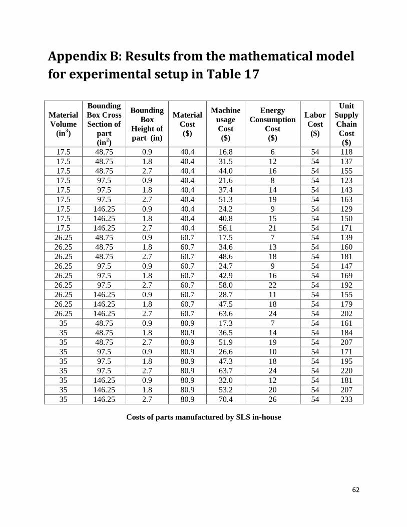
62
Appendix B: Results from the mathematical model
for experimental setup in Table 17
Material
Volume
(in3)
Bounding
Box Cross
Section of
part
(in2)
Bounding
Box
Height of
part (in)
Material
Cost
($)
Machine
usage
Cost
($)
Energy
Consumption
Cost
($)
Labor
Cost
($)
Unit
Supply
Chain
Cost
($)
17.5 48.75 0.9 40.4 16.8 6 54 118
17.5 48.75 1.8 40.4 31.5 12 54 137
17.5 48.75 2.7 40.4 44.0 16 54 155
17.5 97.5 0.9 40.4 21.6 8 54 123
17.5 97.5 1.8 40.4 37.4 14 54 143
17.5 97.5 2.7 40.4 51.3 19 54 163
17.5 146.25 0.9 40.4 24.2 9 54 129
17.5 146.25 1.8 40.4 40.8 15 54 150
17.5 146.25 2.7 40.4 56.1 21 54 171
26.25 48.75 0.9 60.7 17.5 7 54 139
26.25 48.75 1.8 60.7 34.6 13 54 160
26.25 48.75 2.7 60.7 48.6 18 54 181
26.25 97.5 0.9 60.7 24.7 9 54 147
26.25 97.5 1.8 60.7 42.9 16 54 169
26.25 97.5 2.7 60.7 58.0 22 54 192
26.25 146.25 0.9 60.7 28.7 11 54 155
26.25 146.25 1.8 60.7 47.5 18 54 179
26.25 146.25 2.7 60.7 63.6 24 54 202
35 48.75 0.9 80.9 17.3 7 54 161
35 48.75 1.8 80.9 36.5 14 54 184
35 48.75 2.7 80.9 51.9 19 54 207
35 97.5 0.9 80.9 26.6 10 54 171
35 97.5 1.8 80.9 47.3 18 54 195
35 97.5 2.7 80.9 63.7 24 54 220
35 146.25 0.9 80.9 32.0 12 54 181
35 146.25 1.8 80.9 53.2 20 54 207
35 146.25 2.7 80.9 70.4 26 54 233
Costs of parts manufactured by SLS in-house
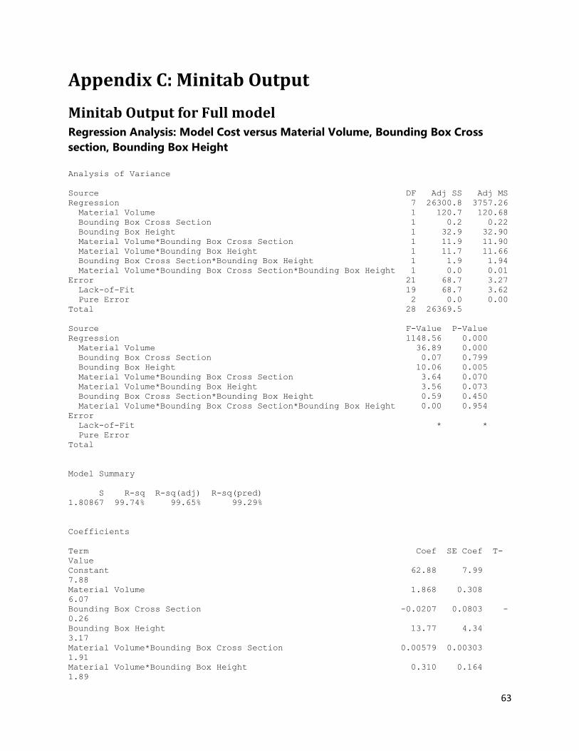
63
Appendix C: Minitab Output
Minitab Output for Full model Regression Analysis: Model Cost versus Material Volume, Bounding Box Cross
section, Bounding Box Height
Analysis of Variance
Source DF Adj SS Adj MS
Regression 7 26300.8 3757.26
Material Volume 1 120.7 120.68
Bounding Box Cross Section 1 0.2 0.22
Bounding Box Height 1 32.9 32.90
Material Volume*Bounding Box Cross Section 1 11.9 11.90
Material Volume*Bounding Box Height 1 11.7 11.66
Bounding Box Cross Section*Bounding Box Height 1 1.9 1.94
Material Volume*Bounding Box Cross Section*Bounding Box Height 1 0.0 0.01
Error 21 68.7 3.27
Lack-of-Fit 19 68.7 3.62
Pure Error 2 0.0 0.00
Total 28 26369.5
Source F-Value P-Value
Regression 1148.56 0.000
Material Volume 36.89 0.000
Bounding Box Cross Section 0.07 0.799
Bounding Box Height 10.06 0.005
Material Volume*Bounding Box Cross Section 3.64 0.070
Material Volume*Bounding Box Height 3.56 0.073
Bounding Box Cross Section*Bounding Box Height 0.59 0.450
Material Volume*Bounding Box Cross Section*Bounding Box Height 0.00 0.954
Error
Lack-of-Fit * *
Pure Error
Total
Model Summary
S R-sq R-sq(adj) R-sq(pred)
1.80867 99.74% 99.65% 99.29%
Coefficients
Term Coef SE Coef T-
Value
Constant 62.88 7.99
7.88
Material Volume 1.868 0.308
6.07
Bounding Box Cross Section -0.0207 0.0803 -
0.26
Bounding Box Height 13.77 4.34
3.17
Material Volume*Bounding Box Cross Section 0.00579 0.00303
1.91
Material Volume*Bounding Box Height 0.310 0.164
1.89

64
Bounding Box Cross Section*Bounding Box Height 0.0329 0.0427
0.77
Material Volume*Bounding Box Cross Section*Bounding Box Height -0.00009 0.00160 -
0.06
Term P-Value VIF
Constant 0.000
Material Volume 0.000 43.99
Bounding Box Cross Section 0.799 92.94
Bounding Box Height 0.005 88.49
Material Volume*Bounding Box Cross Section 0.070 141.20
Material Volume*Bounding Box Height 0.073 135.28
Bounding Box Cross Section*Bounding Box Height 0.450 180.16
Material Volume*Bounding Box Cross Section*Bounding Box Height 0.954 223.77
Regression Equation
Model Cost = 62.88 + 1.868 Material Volume - 0.0207 Bounding Box Cross Section
+ 13.77 Bounding Box Height
+ 0.00579 Material Volume*Bounding Box Cross Section
+ 0.310 Material Volume*Bounding Box Height
+ 0.0329 Bounding Box Cross Section*Bounding Box Height
- 0.00009 Material Volume*Bounding Box Cross Section*Bounding Box Height
Fits and Diagnostics for Unusual Observations
Std
Obs Model Cost Fit Resid Resid
14 173.048 169.483 3.565 2.01 R
23 199.259 195.506 3.753 2.18 R
R Large residual
Minitab Output for Reduced model Regression Analysis: Model Cost versus Material Volume, Bounding Box Cross
Section, Bounding Box Height
Analysis of Variance
Source DF Adj SS Adj MS F-Value P-
Value
Regression 6 26300.8 4383.47 1403.57
0.000
Material Volume 1 455.4 455.37 145.81
0.000
Bounding Box Cross Section 1 0.7 0.68 0.22
0.644
Bounding Box Height 1 161.7 161.72 51.78
0.000
Material Volume*Bounding Box Cross Section 1 77.3 77.27 24.74
0.000
Material Volume*Bounding Box Height 1 71.7 71.68 22.95
0.000
Bounding Box Cross Section*Bounding Box Height 1 22.7 22.75 7.28
0.013
Error 22 68.7 3.12
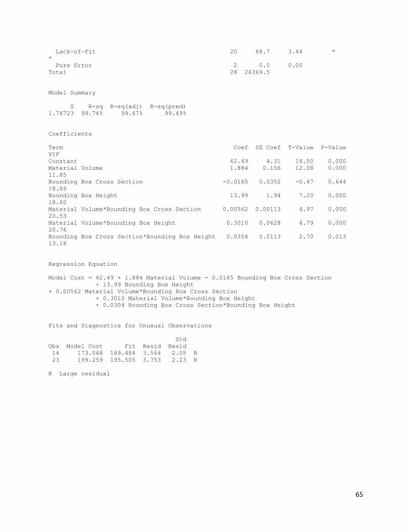
65
Lack-of-Fit 20 68.7 3.44 *
*
Pure Error 2 0.0 0.00
Total 28 26369.5
Model Summary
S R-sq R-sq(adj) R-sq(pred)
1.76723 99.74% 99.67% 99.49%
Coefficients
Term Coef SE Coef T-Value P-Value
VIF
Constant 62.49 4.31 14.50 0.000
Material Volume 1.884 0.156 12.08 0.000
11.85
Bounding Box Cross Section -0.0165 0.0352 -0.47 0.644
18.69
Bounding Box Height 13.99 1.94 7.20 0.000
18.60
Material Volume*Bounding Box Cross Section 0.00562 0.00113 4.97 0.000
20.53
Material Volume*Bounding Box Height 0.3010 0.0628 4.79 0.000
20.76
Bounding Box Cross Section*Bounding Box Height 0.0304 0.0113 2.70 0.013
13.18
Regression Equation
Model Cost = 62.49 + 1.884 Material Volume - 0.0165 Bounding Box Cross Section
+ 13.99 Bounding Box Height
+ 0.00562 Material Volume*Bounding Box Cross Section
+ 0.3010 Material Volume*Bounding Box Height
+ 0.0304 Bounding Box Cross Section*Bounding Box Height
Fits and Diagnostics for Unusual Observations
Std
Obs Model Cost Fit Resid Resid
14 173.048 169.484 3.564 2.05 R
23 199.259 195.505 3.753 2.23 R
R Large residual
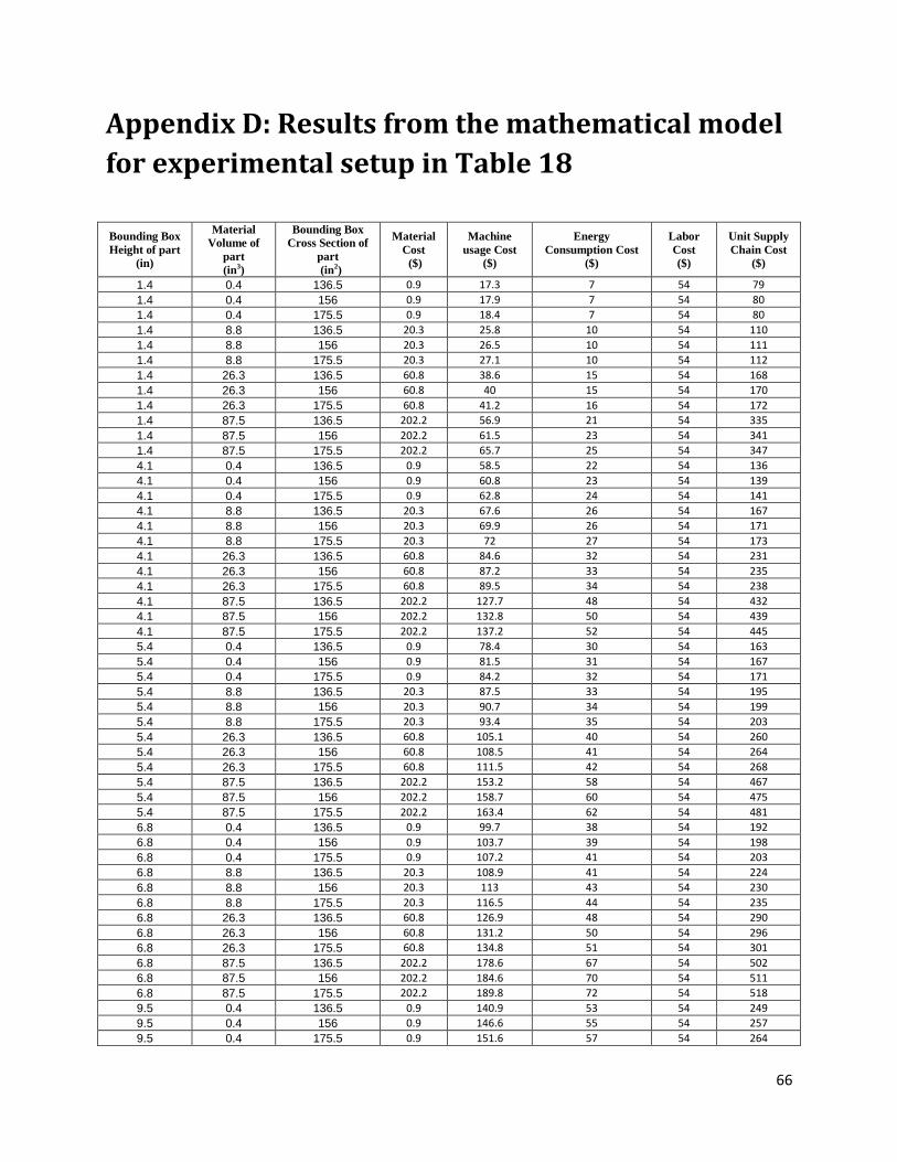
66
Appendix D: Results from the mathematical model
for experimental setup in Table 18
Bounding Box
Height of part
(in)
Material
Volume of
part
(in3)
Bounding Box
Cross Section of
part
(in2)
Material
Cost
($)
Machine
usage Cost
($)
Energy
Consumption Cost
($)
Labor
Cost
($)
Unit Supply
Chain Cost
($)
1.4 0.4 136.5 0.9 17.3 7 54 79
1.4 0.4 156 0.9 17.9 7 54 80
1.4 0.4 175.5 0.9 18.4 7 54 80
1.4 8.8 136.5 20.3 25.8 10 54 110
1.4 8.8 156 20.3 26.5 10 54 111
1.4 8.8 175.5 20.3 27.1 10 54 112
1.4 26.3 136.5 60.8 38.6 15 54 168
1.4 26.3 156 60.8 40 15 54 170
1.4 26.3 175.5 60.8 41.2 16 54 172
1.4 87.5 136.5 202.2 56.9 21 54 335
1.4 87.5 156 202.2 61.5 23 54 341
1.4 87.5 175.5 202.2 65.7 25 54 347
4.1 0.4 136.5 0.9 58.5 22 54 136
4.1 0.4 156 0.9 60.8 23 54 139
4.1 0.4 175.5 0.9 62.8 24 54 141
4.1 8.8 136.5 20.3 67.6 26 54 167
4.1 8.8 156 20.3 69.9 26 54 171
4.1 8.8 175.5 20.3 72 27 54 173
4.1 26.3 136.5 60.8 84.6 32 54 231
4.1 26.3 156 60.8 87.2 33 54 235
4.1 26.3 175.5 60.8 89.5 34 54 238
4.1 87.5 136.5 202.2 127.7 48 54 432
4.1 87.5 156 202.2 132.8 50 54 439
4.1 87.5 175.5 202.2 137.2 52 54 445
5.4 0.4 136.5 0.9 78.4 30 54 163
5.4 0.4 156 0.9 81.5 31 54 167
5.4 0.4 175.5 0.9 84.2 32 54 171
5.4 8.8 136.5 20.3 87.5 33 54 195
5.4 8.8 156 20.3 90.7 34 54 199
5.4 8.8 175.5 20.3 93.4 35 54 203
5.4 26.3 136.5 60.8 105.1 40 54 260
5.4 26.3 156 60.8 108.5 41 54 264
5.4 26.3 175.5 60.8 111.5 42 54 268
5.4 87.5 136.5 202.2 153.2 58 54 467
5.4 87.5 156 202.2 158.7 60 54 475
5.4 87.5 175.5 202.2 163.4 62 54 481
6.8 0.4 136.5 0.9 99.7 38 54 192
6.8 0.4 156 0.9 103.7 39 54 198
6.8 0.4 175.5 0.9 107.2 41 54 203
6.8 8.8 136.5 20.3 108.9 41 54 224
6.8 8.8 156 20.3 113 43 54 230
6.8 8.8 175.5 20.3 116.5 44 54 235
6.8 26.3 136.5 60.8 126.9 48 54 290
6.8 26.3 156 60.8 131.2 50 54 296
6.8 26.3 175.5 60.8 134.8 51 54 301
6.8 87.5 136.5 202.2 178.6 67 54 502
6.8 87.5 156 202.2 184.6 70 54 511
6.8 87.5 175.5 202.2 189.8 72 54 518
9.5 0.4 136.5 0.9 140.9 53 54 249
9.5 0.4 156 0.9 146.6 55 54 257
9.5 0.4 175.5 0.9 151.6 57 54 264
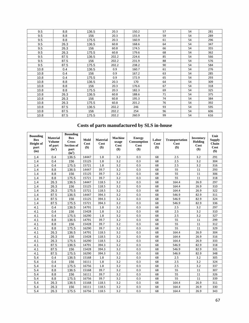
67
9.5 8.8 136.5 20.3 150.2 57 54 281
9.5 8.8 156 20.3 155.9 59 54 289
9.5 8.8 175.5 20.3 160.9 61 54 296
9.5 26.3 136.5 60.8 168.6 64 54 347
9.5 26.3 156 60.8 174.5 66 54 355
9.5 26.3 175.5 60.8 179.6 68 54 362
9.5 87.5 136.5 202.2 224.6 85 54 566
9.5 87.5 156 202.2 231.9 88 54 576
9.5 87.5 175.5 202.2 238.2 90 54 584
10.8 0.4 136.5 0.9 160.7 61 54 276
10.8 0.4 156 0.9 167.2 63 54 285
10.8 0.4 175.5 0.9 172.9 65 54 293
10.8 8.8 136.5 20.3 170 64 54 309
10.8 8.8 156 20.3 176.6 67 54 318
10.8 8.8 175.5 20.3 182.3 69 54 325
10.8 26.3 136.5 60.8 188.6 71 54 375
10.8 26.3 156 60.8 195.3 74 54 384
10.8 26.3 175.5 60.8 201.2 76 54 392
10.8 87.5 136.5 202.2 246 93 54 595
10.8 87.5 156 202.2 254 96 54 606
10.8 87.5 175.5 202.2 260.9 99 54 616
Costs of parts manufactured by SLS in-house
Bounding
Box
Height of
part
(in)
Material
Volume
of part
(in3)
Bounding
Box
Cross
Section of
part
(in2)
Mold
Cost
($)
Material
Cost
($)
Machine
usage
Cost
($)
Energy
Consumption
Cost
($)
Labor
Cost
($)
Transportation
Cost
($)
Inventory
Holding
Cost
($)
Unit
Supply
Chain
Cost
($)
1.4 0.4 136.5 14447 1.8 3.2 0.3 68 2.5 3.2 291
1.4 0.4 156 15125 1.8 3.2 0.3 68 2.5 3.2 304
1.4 0.4 175.5 15721 1.8 3.2 0.3 68 2.5 3.2 316
1.4 8.8 136.5 14447 39.7 3.2 0.3 68 55 11 293
1.4 8.8 156 15125 39.7 3.2 0.3 68 55 11 306
1.4 8.8 175.5 15721 39.7 3.2 0.3 68 55 11 318
1.4 26.3 136.5 14447 118.5 3.2 0.3 68 164.4 26.9 297
1.4 26.3 156 15125 118.5 3.2 0.3 68 164.4 26.9 310
1.4 26.3 175.5 15721 118.5 3.2 0.3 68 164.4 26.9 322
1.4 87.5 136.5 14447 394.3 3.2 0.3 68 546.9 82.9 311
1.4 87.5 156 15125 394.3 3.2 0.3 68 546.9 82.9 324
1.4 87.5 175.5 15721 394.3 3.2 0.3 68 546.9 82.9 336
4.1 0.4 136.5 14791 1.8 3.2 0.3 68 2.5 3.2 297
4.1 0.4 156 15428 1.8 3.2 0.3 68 2.5 3.2 310
4.1 0.4 175.5 16290 1.8 3.2 0.3 68 2.5 3.2 327
4.1 8.8 136.5 14791 39.7 3.2 0.3 68 55 11 299
4.1 8.8 156 15428 39.7 3.2 0.3 68 55 11 312
4.1 8.8 175.5 16290 39.7 3.2 0.3 68 55 11 329
4.1 26.3 136.5 14791 118.5 3.2 0.3 68 164.4 26.9 304
4.1 26.3 156 15428 118.5 3.2 0.3 68 164.4 26.9 316
4.1 26.3 175.5 16290 118.5 3.2 0.3 68 164.4 26.9 333
4.1 87.5 136.5 14791 394.3 3.2 0.3 68 546.9 82.9 318
4.1 87.5 156 15428 394.3 3.2 0.3 68 546.9 82.9 331
4.1 87.5 175.5 16290 394.3 3.2 0.3 68 546.9 82.9 348
5.4 0.4 136.5 15168 1.8 3.2 0.3 68 2.5 3.2 305
5.4 0.4 156 16111 1.8 3.2 0.3 68 2.5 3.2 324
5.4 0.4 175.5 16756 1.8 3.2 0.3 68 2.5 3.2 337
5.4 8.8 136.5 15168 39.7 3.2 0.3 68 55 11 307
5.4 8.8 156 16111 39.7 3.2 0.3 68 55 11 326
5.4 8.8 175.5 16756 39.7 3.2 0.3 68 55 11 339
5.4 26.3 136.5 15168 118.5 3.2 0.3 68 164.4 26.9 311
5.4 26.3 156 16111 118.5 3.2 0.3 68 164.4 26.9 330
5.4 26.3 175.5 16756 118.5 3.2 0.3 68 164.4 26.9 343

68
5.4 87.5 136.5 15168 394.3 3.2 0.3 68 546.9 82.9 325
5.4 87.5 156 16111 394.3 3.2 0.3 68 546.9 82.9 344
5.4 87.5 175.5 16756 394.3 3.2 0.3 68 546.9 82.9 357
6.8 0.4 136.5 15542 1.8 3.2 0.3 68 2.5 3.2 313
6.8 0.4 156 16237 1.8 3.2 0.3 68 2.5 3.2 326
6.8 0.4 175.5 17409 1.8 3.2 0.3 68 2.5 3.2 350
6.8 8.8 136.5 15542 39.7 3.2 0.3 68 55 11 314
6.8 8.8 156 16237 39.7 3.2 0.3 68 55 11 328
6.8 8.8 175.5 17409 39.7 3.2 0.3 68 55 11 352
6.8 26.3 136.5 15542 118.5 3.2 0.3 68 164.4 26.9 319
6.8 26.3 156 16237 118.5 3.2 0.3 68 164.4 26.9 332
6.8 26.3 175.5 17409 118.5 3.2 0.3 68 164.4 26.9 356
6.8 87.5 136.5 15542 394.3 3.2 0.3 68 546.9 82.9 333
6.8 87.5 156 16237 394.3 3.2 0.3 68 546.9 82.9 347
6.8 87.5 175.5 17409 394.3 3.2 0.3 68 546.9 82.9 370
9.5 0.4 136.5 16228 1.8 3.2 0.3 68 2.5 3.2 326
9.5 0.4 156 17550 1.8 3.2 0.3 68 2.5 3.2 353
9.5 0.4 175.5 18211 1.8 3.2 0.3 68 2.5 3.2 366
9.5 8.8 136.5 16228 39.7 3.2 0.3 68 55 11 328
9.5 8.8 156 17550 39.7 3.2 0.3 68 55 11 355
9.5 8.8 175.5 18211 39.7 3.2 0.3 68 55 11 368
9.5 26.3 136.5 16228 118.5 3.2 0.3 68 164.4 26.9 332
9.5 26.3 156 17550 118.5 3.2 0.3 68 164.4 26.9 359
9.5 26.3 175.5 18211 118.5 3.2 0.3 68 164.4 26.9 372
9.5 87.5 136.5 16228 394.3 3.2 0.3 68 546.9 82.9 347
9.5 87.5 156 17550 394.3 3.2 0.3 68 546.9 82.9 373
9.5 87.5 175.5 18211 394.3 3.2 0.3 68 546.9 82.9 386
10.8 0.4 136.5 16355 1.8 3.2 0.3 68 2.5 3.2 329
10.8 0.4 156 17705 1.8 3.2 0.3 68 2.5 3.2 356
10.8 0.4 175.5 18365 1.8 3.2 0.3 68 2.5 3.2 369
10.8 8.8 136.5 16355 39.7 3.2 0.3 68 55 11 331
10.8 8.8 156 17705 39.7 3.2 0.3 68 55 11 358
10.8 8.8 175.5 18365 39.7 3.2 0.3 68 55 11 371
10.8 26.3 136.5 16355 118.5 3.2 0.3 68 164.4 26.9 335
10.8 26.3 156 17705 118.5 3.2 0.3 68 164.4 26.9 362
10.8 26.3 175.5 18365 118.5 3.2 0.3 68 164.4 26.9 375
10.8 87.5 136.5 16355 394.3 3.2 0.3 68 546.9 82.9 349
10.8 87.5 156 17705 394.3 3.2 0.3 68 546.9 82.9 376
10.8 87.5 175.5 18365 394.3 3.2 0.3 68 546.9 82.9 389
Costs of parts manufactured by IM at central location