a method to control turbofan engine starting by varying
TRANSCRIPT

A METHOD TO CONTROL TURBOFAN ENGINE STARTING BY
VARYING COMPRESSOR SURGE VALVE BLEED
Wayne Randolph Sexton
Thesis submitted to the Graduate Faculty of the Virginia Polytechnic Institute and State University
in partial fulfillment of the requirements of the degree of
MASTER OF SCIENCE
In
Mechanical Engineering
Dr. Walter F. O'Brien Dr. Peter S. King Dr. Wing F. Ng
May 14, 2001 Blacksburg Virginia
Keywords: turbomachinery characteristic extrapolation, engine simulation, gas turbine engine starting, bleed valve

Acknowledgements “Good, better, best; never rest until your good is better than best.”
-author, unknown
The Mechanical Engineering Department at Virginia Tech is an excellent and
privileged institution. For mechanical engineering students and faculty, the corporate
sponsorship, funding, and involvement is second-to-none. The analytical and experimental
research tools that are at a graduate student’s and faculty member’s disposal are made
available by corporations who trust Virginia Tech’s reputation for being a renowned
engineering research center.
The work reported for this research was made possible by research tools donated by
NASA, and subsequently supported by Honeywell Corp. to the Mechanical Engineering
Department. They have given Virginia Tech a gas turbine turbofan engines with generous
technical support. I would like to thank Tom Cunningham, John Harvell, Phil Dury, Matt
Sandifur, and Ed Palmerueter for their considerable help on many areas during this
research. Honeywell has also entrusted the Mechanical Engineering Department with their
proprietary gas turbine engine performance program, FAST, for research and teaching
uses.
I would like to thank Major Dave Bossert and Jerry Stermer at the Air Force
Academy for selfless help to me in modifying their engine test stand data acquisition
system to collect low speed starting data.
I would like to thank my committee, Dr. W. F. O'Brien, Dr. P. S. King, and Dr. W.
F. Ng for their tireless guidance and wisdom.
Thank you Mike and Julia, Pauline, Mom and Dad, Grandma and Grandpa, for
being there for me. A special thanks to my father, who I believe genetically instilled a
strong disposition and love for mechanical engineering and turbomachinery.
ii

Contents
Acknowledgements………………………………………………………….…………….ii Contents………………………..………..……..…………………………………………iii Abstract…...……………………………………………………………………………….v List of Figures…………………….…………………………………………...……....…vi List of Symbols……………………………………………………………………..…....ix 1. Introduction…………………..………………………………..…..…….………...……..1 2. Literature Review………………………..……………………….……….……...….…...4
2.1 Engine Starting and Associated problems...………………………..……..…….4 Surge………………………………………………………………..…….……..6 Stall………………………………………………………………..…….………6
2.2 Component Characteristics for Low Speed Simulation…………….…….….…9
3. Research Tools………………………………………………………………….………12 .
3.1 The Turbofan Engine………………………………………………….………12
3.2 Computer Simulation Program……….……...……….……………..…………13 4. Map Extrapolation……..………..………………………………………………..……..14
4.1 Characteristic Map Formatting…………………………………………..…..14 4.2 Background to Developed Extrapolation Method……………….…………..18 4.3 Development of Extrapolation Method….……………………….………….21 Turbine Maps..…………………………………………………….………..21 Fan and Compressor Maps…………………………………………….……49
5. Comparison of Simulated Starting Results with Experimental Data…………….……..67 6. Surge Valve Variable Area Results……………………..……………...…..…..……….75
6.1 Equilibrium Running Lines for Varying Valve Area………...……………..…75
iii

6.2 Parametric Study of Varying Valve Area………………………………….….81 6.3 Surge Valve Area Schedule……………………………………………..….…84
7. Conclusions………..…………………..…………………………………………..……94 8. Recommendations……………………..…………………………………………..……95 References…..……………...……………………………………………..…………….....96 Appendices…………….………………………………………………….....…………….97
Appendix A. Discussion of Agrawal and Yunis Extrapolation Method………..…97 Appendix B. MatLab Script File Names and Availability..……………………...102
Vita……………………………………………………………………………………….103
iv
A METHOD TO CONTROL TURBOFAN ENGINE STARTING BY VARYING COMPRESSOR SURGE VALVE BLEED
Wayne R. Sexton
(ABSTRACT)
This thesis reports the results of a study of the starting conditions of a turbofan
engine. The research focused on ways to minimize turbine inlet temperature while maintaining an adequate compressor stall margin during engine start by varying the surge valve bleed. Varying the surge valve bleed was also shown to reduce compressor and fan required torque.
A new method of turbofan engine component characteristic map extrapolation was
developed. This novel method uses incompressible similarity laws, but compressibility effects of the flow are reflected by changing the exponent used in the similarity laws. These extrapolated component characteristic maps were tested in a simulation of the turbofan engine by stepping engine speed from close to ignition speed to idle speed. The simulation predictions were verified by comparing them to experimental engine performance data.
Lastly, a parametric study of starting surge valve flow area schedule was performed
to reduce turbine temperatures while maintaining adequate stall margin. Minimizing turbine inlet temperatures during start-up when turbine components are cold will minimize thermal shock and thereby extend turbine component life.
v

List of Figures Figure 3-1. Cut-away of the turbofan engine modeled for starting research.…………….13 Figure 4-1. Compressor Map with one beta line………………………………………….15 Figure 4-1A. Pressure Ratio Beta Map from Compressor Map………………………….16 Figure 4-1B. Corrected Mass Flow Beta Map from the Compressor Map……………….16 Figure 4-2. Low Pressure Compressor Referred Airflow Beta Map……………………..17 Figure 4-3. High Pressure Turbine Referred Airflow Beta Map…………………………22 Figure 4-4. High Pressure Turbine Referred Airflow Conventional Map……………….24 Figure 4-5. HP Turbine Corrected Torque Map with 50% & 60% map lines and 50% similar line…………………………………………………………………….35 Figure 4-6. HP Turbine Corrected Torque Map with Extrapolated Speed Lines..…..……36 Figure 4-7. HP Turbine Referred Airflow Map with Extrapolated Speed Lines..….…….37 Figure 4-8. LP Turbine Corrected Torque Map with Extrapolated Speed Lines………....38 Figure 4-9. LP Turbine Referred Airflow Map with Extrapolated Speed Lines………….39 Figure 4-10. HP Turbine Efficiency Map with Extrapolated Speed Lines...……………..41 Figure 4-11. LP Turbine Efficiency Map with Extrapolated Speed Lines………………..42 Figure 4-12. HP Turbine Referred Airflow Map with Extended Speed Lines……………43 Figure 4-13. HP Turbine Corrected Torque Map with Extended Speed Lines…………...44 Figure 4-14. LP Turbine Referred Airflow Map with Extended Speed Lines……….…...45 Figure 4-15. LP Turbine Corrected Map with Extended Speed Lines……………………46 Figure 4-16. HP Turbine Efficiency Map with Extended Speed Lines…………………..47 Figure 4-17. LP Turbine Efficiency Map with Extended Speed Lines.…………………..48 Figure 4-18. Fan Hub (Core) Pressure Ratio map with Extrapolated Speed Lines……….52
vi

Figure 4-19. Fan Tip (Bypass) Pressure Ratio map with Extrapolated Speed Lines……..53 Figure 4-20. Low Pressure Compressor Pressure Ratio map with Extrapolated Speed Lines………………………………………………………………….54 Figure 4-21. High Pressure Compressor Pressure Ratio map with Extrapolated Speed Lines………………………………………………………………….55 Figure 4-22. Fan Hub (Core) Efficiency map with Extrapolated Speed Lines…………..58 Figure 4-23. Fan Tip (Bypass) Efficiency map with Extrapolated Speed Lines………….59 Figure 4-24. Low Pressure Compressor Efficiency map with Extrapolated Speed Lines………………………………………………………………….60 Figure 4-25. High Pressure Compressor Efficiency map with Extrapolated Speed Lines………………………………………………………………….61 Figure 4-26. Demonstration of zero speed, flow greater than zero, and pressure ratio less than one………………………………………………………………….…62 Figure 4-27. Fan Hub (Core) Pressure Ratio map with Extended Speed Lines…………..63 Figure 4-28. Fan Tip (Bypass) Pressure Ratio map with Extended Speed Lines………...64 Figure 4-29. Low Pressure Compressor Pressure Ratio map with Extended Speed Lines………………………………………………………………….65 Figure 4-30. High Pressure Compressor Pressure Ratio map with Extended Speed Lines………………………………………………………………….66 Figure 5-1. Schematic of the turbofan engine modeled for starting research…………….68 Figure 5-2. PS3/Pamb as a function of percent of design high speed shaft..……………..69 Figure 5-3. PT3/Pamb as a function of percent of design high speed shaft..……………..70 Figure 5-4. θ45 as a function of percent of design high speed shaft...…………………….72 Figure 5-5. Design low speed shaft as a function of percent of design high speed shaft....74 Figure 6-1. Fan Hub Pressure Ratio map with 0.26in2 Valve Area Equilibrium running line.……..…………………….………………………………………….…...77 Figure 6-2. Fan Tip Pressure Ratio map with 0.26in2 Valve Area Equilibrium running line……………………………………………………………………….…...78
vii

Figure 6-3. Low Pressure Compressor Pressure Ratio map with 0.26in2 Surge Valve Area Equilibrium running line……….………………………………………….….79 Figure 6-4. Low Pressure Compressor Pressure Ratio map with various Surge Valve Area Equilibrium running lines……………………………………………….……80 Figure 6-5. Low Pressure Compressor Surge Margin as a function of percent of design high-speed shaft speed and valve area……………………………………….82 Figure 6-6. θ41 as a function of percent of design high-speed shaft speed and valve area..83 Figure 6-7. Low Pressure Compressor Power as a function of percent of design high-speed shaft speed and valve area….…………………………………………………85 Figure 6-8. High Pressure Compressor Power as a function of percent of design high- speed shaft speed and valve area…………..…………………………………86 Figure 6-9. Variable valve schedule surge margin superimposed on the parametric plot of the LP compressor surge margin……………………………………………..87 Figure 6-10. Variable valve area schedule comparison to fixed valve area………………88 Figure 6-11. Variable valve area schedule surge margin comparison to fixed valve area surge margin………………………………………………………………...90 Figure 6-12. Variable valve schedule θ41 superimposed on the parametric plot of θ41…...91 Figure 6-13. Variable valve area schedule θ41 comparison to fixed valve area θ41….…...92 Figure 6-14. Variable valve area schedule LP compressor power comparison to fixed valve area LP compressor power…………………………………………...93
viii

List of Symbols
CP constant pressure specific heat
CZ axial velocity m& mass flow rate N rotational speed N1 low-speed spool rotational
speed N2 high-speed spool
rotational speed NMAX component maximum
rotational speed %NRFRD percent referred N Pamb standard pressure P0 total pressure Pr pressure ratio PS static pressure Pwr power Rg gas constant for
combustion products Tamb standard temperature T0 total temperature Tq torque TS static temperature
U blade velocity W work δ P0/Pamb φ flow coefficient γ specific heat ratio
η efficiency ρ density θ T0/Tamb subscripts: C fan/compressor i inlet condition MAP engine manufacture's
component map
NEW extrapolated line
REF reference line
T turbine
ix

CHAPTER 1
Introduction
This thesis reports the results of a study of the starting conditions of a turbofan
engine. The engine modeled in this work was not a production engine and is not currently
used on any private, commercial, or government owned aircraft.
The starting procedure for a gas turbine engine usually only lasts a minute or two
depending on the size of the engine. However, during this starting time there are many
interactions occurring between the working fluid and the mechanical components of the
engine. There are many interesting topics in these component and fluid interactions for
research, which may result in overall engine performance improvements. Some of the
parameters of interest during engine starting are the turbine temperature, the compressor
stall margin, and the required torque.
The research reported here focused on minimizing the turbine temperature while
maintaining an adequate compressor stall margin during engine start by varying the surge
valve bleed. It is always important to consider the turbine temperature during the starting
and acceleration processes. Turbine blades are designed to operate at high temperatures,
but their life is limited by heat stress caused by rapid temperature increases, especially
when starting from cold initial conditions. The stress caused by steep temperature
gradients can lead to micro-cracks, fatigue, and ultimately failure. Another benefit of
varying surge valve bleed may be the reduction of compressor and fan torque. This
reduction in torque may reduce wear on the starter motor and mechanical systems
necessary to accelerate the engine to self-sustaining speeds.
This research was completed in three distinct phases. Phase one required the
extrapolation of the turbofan engine component maps into the low speed region. These
low speed maps were necessary for the engine simulation to be run at the low start-up
speeds. Phase two tested, adjusted, and verified that the new maps correctly simulated the
1

engine performance in the low speed range. The simulation predictions were verified by
comparing them to experimental engine performance data. Phase three was a parametric
study of starting surge valve bleed schedules to reduce turbine temperatures while
maintaining adequate stall margin.
Originally, an extrapolation method from the literature was thought to be useful for
the beta format of the component characteristic maps. This method, however, was not
applicable for the data provided with this turbofan engine. Next, consideration was given
to constructing an extrapolation method similar to that used by the engine manufacturer.
The engine manufacturer's method relies heavily on the experience of the analyst in
estimating component efficiencies. Without this experience and all of the details of the
engine manufacturer's method, the researcher did not feel comfortable applying this
method. Therefore, a new method of map extrapolation was developed. This new method,
which is somewhat novel when compared to the method found in the literature, uses
incompressible similarity laws (similar to the familiar pump laws) but compressibility
effects of the flow are reflected by changing the exponent of these similarity laws.
Contrary to the extrapolation method discussed in the literature, the method developed here
uses more conventional component map format as opposed to the beta format. After
extrapolation the maps were returned to the beta format for use in the current engine
model.
In phase two, these extrapolated component characteristic maps were tested in the
model by stepping engine speed down from idle speed to close to ignition speed. The
simulation model predicts a quasi-steady equilibrium running line, that is, a series of
steady state operating points. The equilibrium running line produced using the engine
performance code, and the new low speed component characteristic, showed that the
simulated start-up results compared favorably with experimentally measured start-up
conditions. There were two sets of experimental starting data available, one from the
engine manufacturer's initial tests and the second from the Air Force Academy. The
simulation showed very similar trends during start-up in combustion pressures, turbine
temperatures, shaft speeds, and thrust as compared to the experimental data. Since turbine
2

temperatures and stall margin were the main focus of the research, the simulation was run
up from near ignition speed (high-speed shaft 10,000 RPM, low-speed shaft less than 100
RPM). Prior to ignition the starter motor is primarily overcoming the shaft and component
inertias. Relative to the core flow, even just after ignition, the flow through the surge valve
is very small. Therefore, changing the surge valve bleed prior to ignition may have little
influence on turbine temperatures and stall margin.
Phase three was a parametric study of starting surge valve bleed schedules to
reduce turbine temperatures while maintaining adequate stall margin. This was
accomplished by varying surge valve flow area. The actual turbofan engine has a fixed
area surge valve. This surge valve was sized to insure an adequate stall margin at very low
speeds where there is little concern about turbine temperatures. However, at higher speeds
this fixed area surge valve will allow a larger bleed flow that will increase the stall margin
at the expense of increased turbine inlet temperatures. This investigation into a new surge
valve schedule showed that a sufficient stall margin could be maintained while limiting the
turbine inlet temperature by changing the area of the surge valve during the engine start-
up. Minimizing turbine inlet temperatures during start-up, when turbine components are
cold, will minimize thermal shock of turbine components and thereby extend turbine
component life.
3

CHAPTER 2
Literature Review
The research reported here was an analytical study of a twin-spool turbofan engine
start-up. The first section of this literature review describes engine starting and the
associated problems. The second section describes techniques to extrapolate low-speed
component characteristics from characteristics in the normal operating range.
2.1 Engine Starting and Associated Problems
What is involved in starting a gas turbine engine? Walsh and Fletcher [1]
described a sequence of steps that need to be strictly followed to ensure a successful engine
start. The steps are purging, dry cranking, combustor ignition, and engine acceleration.
Purging of the engine occurs as the starter begins to rotate the high-speed spool and
its components. As these components begin to rotate they draw air through the engine.
This initial airflow evacuates any combustible fumes that may have been trapped during
previous failed starts or from a flameout during engine operation. A premature
combustion due to trapped combustibles could damage engine components from the
sudden pressure and/or temperature rise.
For a short time during engine starting the starter motor rotates the gas generator
during a phase of dry cranking where fuel is not combusted. The term dry cranking is a
little misleading. Most often fuel is being added during this time to prime the combustor.
During dry cranking the starter motor accelerates the engine components. As the engine
begins to rotate faster the starter motor continues to accelerate the high-speed shaft until
the compressor pressure ratio and airflow are sufficient to sustain combustion in the
combustor.
4

Once fuel is being continuously added and the compressors are developing enough
boost and airflow, the combustor is ignited and the engine can continue to accelerate on its
own. However, the starter is not yet disengaged. The starter continues until the torque
supplied by the turbine stages is approximately equal to the torque supplied by the starter.
There are two reasons why the starter continues to run until the turbine and starter motor
torques are approximately equal. First, there is some time after ignition when the engine
can get trapped in “hung stall”. Hung stall is a phenomenon in which regardless of how
much fuel is added the engine will not accelerate on its own. The starter provides the
required torque to continue engine acceleration and avoid hung stall. Second, the starter
continues to run until it no longer adds torque. At this point the engine is self-sustaining
and can be accelerated by adding more fuel to the combustor.
Cohen, et al. [2] described how the two shafts of a twin-spool gas turbine engine
operate together during normal acceleration, deceleration, and steady state operation.
During engine starting the problems associated with low flow, low speed off-design
operation are compounded by engine acceleration. Walsh and Fletcher took the concepts
introduced by Cohen, et al. a step further and described this off-design acceleration and
twin-spool interaction at the very low speeds encountered during starting.
The problems associated with starting are mitigated by the use of variable guide
vanes or bleed valves in current gas turbine engine designs. Walsh and Fletcher examined
the interactions of the components of the two engine spools in order to determine what was
actually taking place in an engine when the pilot or operator starts the engine. They
explained that the low-speed spool would begin to rotate when there was sufficient
pressure drop and airflow. This flow results from the increasing suction due to the driven
high-speed shaft compressor. They found that since the components are linked only by
aerodynamics, the high-speed shaft and its components must be accelerated rapidly so as to
draw enough air though the low-pressure components so that the low-speed shaft can
overcome the static friction in its bearings and seals. When the low-speed shaft has
overcome its static friction, the shaft and its components will begin to rotate. Therefore,
during the initial phases of engine start-up, there is some time period where the high-speed
5

spool is rotating and the low-speed spool is not. There may be a pressure drop across the
low-pressure compressor, or fan depending on the design, even after it has started to rotate.
At very low-speed operation this pressure drop can be tolerated as the low-pressure
compressor and/or fan contributes little to the actual starting of the engine.
Several authors have described the problems related to the stall and surge of
compressors that may occur during engine start-up. The problems of stall and surge occur
in engines having axial-flow and/or centrifugal-flow compressors (Aungier [3] and Wilson
[4]). These authors also describe some techniques that are currently used to mitigate the
effects of stall and surge during engine start-up.
Surge. Surge is a flow disturbance that results in cyclic forward/reverse flow that can
blow out the combustor’s flame during engine operation. It may also inhibit the initiation
of combustion during engine start-up. In either case, severe component cyclic fatigue may
occur. For proper engine operation, surge must be avoided. In order to avoid the
possibility of surge, an adequate surge margin must be maintained both during engine
start-up and during normal operation.
Stall. Starting a gas turbine engine encompasses many unique features found only in off-
design performance. The conditions through which the engine passes as it accelerates to
normal operating conditions are far from design. When starting an engine compressor
blade, for axial-flow compressors, or impeller, for centrifugal compressors, stall is likely
due to the off-design conditions associated with low flows and low speeds. Stall, like
surge, is an undesired flow disturbance. But, unlike surge, stall does not have the same
detrimental effects. Any stalled region in the compressor will limit the airflow needed for
engine operation. If the flow through the compressor passages stalls, the mass flow rate of
air is restricted and the compressor will not be able to operate at its design pressure ratio.
Since some stall is usually unavoidable during starting, a rapid acceleration of the engine
through this stalled flow region is desirable.
Hill and Peterson [5] discuss two types of compressor stall. They showed that
compressors could stall due to either a large positive angle of attack or a large negative
6

angle of attack on the compressor blades or impeller. The pressure ratio obtained in the
compressor is limited the stalled region developed by either of these large angles of attack.
Hill and Peterson explained that the inability of a compressor to increase the pressure when
the front stages are stalled causes the density of the air in the latter stages to be too low,
and thus the stalled region progresses farther into the compressor. This low density air
results in an increase in axial velocity in order to move the same mass flow rate of air
through the latter stages. Increasing the axial velocity decreases the angle of attack and the
flow separates from the pressure side of the blade; this is known as negative stall. With
positive stall the same principle of mass flow conservation applies. However, for low axial
inlet velocities, the angle of attack is increased and the flow separates on the suction side
of the blade.
Wilson [4] addressed the problems of stall in multi-stage axial and series-
centrifugal compressors. Wilson stated that the particular compressor stages that stall are
determined by the inlet conditions, in particular the flow coefficient. The flow coefficient,
φ, is defined by Equation 2.1 where CZ is the axial velocity through the compressor and U
is the compressor blade velocity.
UCz=φ (2.1)
The flow coefficient determines the angle of attack on the compressor. A high flow
coefficient will result in a negative angle of attack. Conversely, a low flow coefficient will
result in a positive angle of attack.
Wilson discussed how changing the flow coefficient could shift the stalled stages
between the rear and the front of the compressor section. Wilson stated that if the inlet
design flow coefficient is achieved at low speeds, the front stages will have the design
angle of attack and the latter stages will have negative angles of attack. This is due to the
fact that the front stages are operating at low speeds and therefore these stages will not
7

produce their design pressure rise. This causes the density increase of these stages to be
reduced. This lower density causes the latter stages to have a higher flow coefficient. This
high flow coefficient may drive the latter stages into negative stall. Wilson continued by
explaining that while operating at low speeds a flow coefficient lower than design will
increase the angle of attack on the front stages and may drive these stages into positive
stall. Either of these low-speed flow conditions may occur during engine start-up.
Wilson continued his discussion by describing the effects of flow coefficients at
higher speeds. These high-speed flow conditions may occur during an in-flight engine re-
start. For flow coefficients higher than design, the latter stages may be driven into
negative stall. The difference between low and high-speed operation is that the front
stages at high speeds do not usually stall. When the flow coefficient is below the design
value, there is potential for the rear stages to develop a positive stall.
The mechanical components of the twin-spool gas turbine engine are coupled
aerodynamically and blade stall may determine if a successful start will occur. Though
some stalled regions are always present during engine starting, there are several techniques
used to minimize the detrimental effects of this stall. Walsh and Fletcher [1] proposed
three techniques for minimizing starting stall problems. One of these techniques is the use
of variable inlet guide vanes (VIGVs) at the entrance to the first compressor stage.
Mechanically similar to VIGV's, variable stators are used between stages. A third solution,
as an alternative to the complex mechanisms of variable guide vanes and stators, is the use
of bleed valves. Bleed valves can be divided into two categories, downstream bleed valves
and inter-stage bleed valves.
All three of these solutions differ as to their effects on compressor and engine
operation. Bleed valves downstream of the compressor do not change the characteristic
map of the compressor as occurs when variable stator or VIGV's are used. Because of the
inherent design feartures of centrifugal compressors, only the use of downstream bleeds is
practical. It is possible, however, to bleed between centrifugal compressors in a series-
centrifugal compressor engine such as the turbofan engine modeled in this work.
8

Although, a bleed valve is located between the centrifugal compressors in a series-
centrifugal compressor it is still acting as a downstream bleed valve for the upstream
compressor. Opening of the bleed valve increases the surge margin of the upstream
compressor. Opening the bleed valve moves the equilibrium running line down and away
from the surge line on the compressor characteristic map. However, the resulting reduced
airflow through the engine causes an increase in the turbine inlet temperature.
Unlike centrifugal compressors, axial-flow compressors can have inter-stage
bleeding, that is, a bleed valve located between blade rows. The use of VIGVs
accompanied with variable stators or the use of inter-stage bleed valves will alter the
compressor characteristics requiring a different compressor map to describe operation
during start-up.
Further discussion of gas turbine engine starting can be found in a paper by Wilkes
and O’Brien [6].
2.2 Component Characteristics for Low Speed Simulation
Authors Cohen, et al., Hill and Peterson, Wilson, and Walsh and Fletcher have
related stall and surge phenomena to the starting process. They have suggested solutions
to these starting problems and have described how the engine components behave at low
flow and speeds. However, characteristic maps of components rarely show the low speed
region. Because of the unsteady nature of low speed conditions, characteristic mapping is
difficult. There have been analytical methods proposed by some researchers that may be
used to simulate engine operation during the low speed, low flow conditions associated
with engine starting. The emphasis of the current research was to use these techniques to
develop necessary low speed, low flow fan, compressor, and turbine maps. For that
reason, a method to extrapolate turbomachinery component performance down to the
starting speed range was needed before a starting simulation could be performed.
9

Agrawal and Yunis [7] developed a mathematical model to simulate the start-up of
a gas turbine engine. They began by building the steady state component (compressor,
combustor, and turbine) characteristics. They accomplished this by using the fundamental
relationships of fluid mechanics and other empirical relationships.
Agrawal and Yunis used beta maps to describe component performance
characteristics more simply. These beta maps are similar to the ones that are used in the
proprietary code used in this work. Beta maps expand a single performance map into a
group of simpler maps that have only one parameter (efficiency, pressure ratio, mass flow,
etc.) as a function of speed. A beneficial advantage to having the simpler beta map format
is that when the simulation program is interpolating between points it does not encounter
the steep slopes and discontinuous areas that a conventional map may have.
The other advantage to the Agrawal and Yunis method is that the low speed
characteristics are derived from the well developed normal operation range of the
component characteristic maps. Free of complicated multi-ordered calculations, the
equations they used to derive the low speed characteristics came from the fundamental
definitions of mass flow, work, and efficiency. For a detailed discussion of the Agrawal
and Yunis method, see Appendix A.
A paper written by Kurzke [8] confirms the method of map extrapolation that
Agarwal and Yunis used for their starting simulation. Kurzke, however, showed how the
beta maps are supposed to look at very low speeds. Kurzke showed that when the maps
are correctly extrapolated, there is flow through a low-pressure compressor or fan before
these components start rotating. Walsh and Fletcher described the same results using
conventional compressor characteristic maps. Intuitively, to have a flow drawn through a
compressor or fan requires a low pressure on the backside of that component, hence a
pressure drop through that component. Kurzke’s work agrees with the work of Agarwal
and Yunis in map extrapolation and also confirms the low speed characteristics described
by Walsh and Fletcher.
10

The work of Agarwal and Yunis, Walsh and Fletcher, and Kurzke was used
extensively as a guide in the development of the extrapolation method used in this work.
11

CHAPTER 3
Research Tools
3.1 The Turbofan Engine
The turbofan engine modeled in the current research is shown in Figure 3-1. It is a
twin-spool axial-centrifugal turbofan engine. There are two centrifugal compressors on the
clockwise rotating high-speed spool; the first is designated as the low-pressure (LP)
compressor, and the second, as the high-pressure (HP) compressor. A two-stage axial-flow
HP turbine drives the high speed shaft. Like the high-speed shaft, a two-stage axial-flow
turbine drives the counter-clockwise rotating low speed shaft. The turbine stages on the
low-speed shaft operate at lower pressures. This LP turbine drives the fan at the front of
the engine that draws 52.3 lbs/sec (design) of air into the engine core and bypass duct with
a 5:1 bypass ratio. The combustor is of reverse flow design. The reverse flow design
helps to shorten the overall length of the engine by placing the combustor over the HP
turbine. This design arrangement consists of a length of duct from the exit of the HP
compressor and a 180o turn into the entrance of the combustor, so that the flow is reversed
with respect to the direction it came from the compressor. Then, from the exit of the
combustor there is another 180o turn duct that takes the hot combustion gases into the inlet
of the high-pressure turbine.
There are no variable geometry vanes on the turbofan engine compressors,
therefore, starting stall problems are addressed with a surge valve located between the LP
compressor and HP compressor. All of these design characteristics give the turbofan
engine a compact length of 45 inches with a minimal frontal diameter of 24 inches. The
turbofan engine produces 1330 lbf of thrust and has a specific fuel consumption of 0.396
lbm/hr/lbf at standard, sea-level, take-off conditions [9].
12

Figure 3-1. Cut-away of the turbofan engine modeled for starting research.
3.2 Computer Simulation Program
The basic operation of the gas turbine engine performance computer code requires
the user to prepare a model of the engine for simulation. The model is a component-by-
component list that describes the characteristics and mathematically links the engine
components as they are mechanically linked in the engine to be simulated. At the end of
the model the user define the operating conditions of the engine such as ambient
temperature, pressure, altitude, etc. The user also specifies an engine parameter, such as
speed, that is to be maintained. When the model has been prepared, the gas turbine engine
performance computer code is executed. The gas turbine engine performance computer
code reads the model and operating conditions, performs the gas turbine engine simulation
calculations, and then prints the performance parameters that the user defined in the model.
13

CHAPTER 4
Map Extrapolation
For realistic gas turbine engine starting and low speed performance simulation, it is
important that full component characteristic maps be available for the simulation.
Unfortunately, most characteristic maps do not show the characteristics for speeds below
engine idle. Generally, for gas turbine engines, idle speed is between 40% and 50% of
full design speed. Since the characteristic maps are typically incomplete in this low speed,
low flow area, performance predictions must be based on what can be deduced from
characteristic maps for the components in the normal operating range (idle to full power).
Calculations to predict low speed component performance characteristics must be made
using known physical relationships. Fortunately, the laws of thermodynamics and
conservation laws of fluid mechanics can be manipulated to estimate the steady state
characteristics of engine components at low operating speeds. Therefore, it is possible to
have a physics-based method to reliably predict component characteristics at low speeds
and low flows.
4.1 Characteristic Map Formatting
Before beginning the discussion of map extrapolation it is necessary to describe the
map format, called beta maps, used in the current computer simulation. Conventional
maps for gas turbine engine components are easily interpreted, however, these maps are
difficult to use in a computer simulation due to their steep gradients and multiple
independent variables. Beta maps were developed as a technique to reduce conventional
component characteristic maps into a number of simpler maps. More maps are required
for the beta format because they take the variables on a conventional map and split them
into maps that contain only one dependent variable as a function of one independent
variable. For fans, compressors, and turbines the independent variable used is generally
14
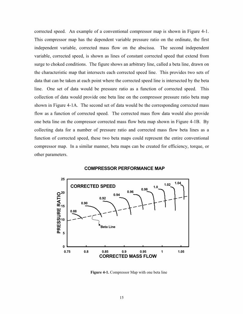
corrected speed. An example of a conventional compressor map is shown in Figure 4-1.
This compressor map has the dependent variable pressure ratio on the ordinate, the first
independent variable, corrected mass flow on the abscissa. The second independent
variable, corrected speed, is shown as lines of constant corrected speed that extend from
surge to choked conditions. The figure shows an arbitrary line, called a beta line, drawn on
the characteristic map that intersects each corrected speed line. This provides two sets of
data that can be taken at each point where the corrected speed line is intersected by the beta
line. One set of data would be pressure ratio as a function of corrected speed. This
collection of data would provide one beta line on the compressor pressure ratio beta map
shown in Figure 4-1A. The second set of data would be the corresponding corrected mass
flow as a function of corrected speed. The corrected mass flow data would also provide
one beta line on the compressor corrected mass flow beta map shown in Figure 4-1B. By
collecting data for a number of pressure ratio and corrected mass flow beta lines as a
function of corrected speed, these two beta maps could represent the entire conventional
compressor map. In a similar manner, beta maps can be created for efficiency, torque, or
other parameters.
COMPRESSOR PERFORMANCE MAP
0
5
10
15
20
25
0.75 0.8 0.85 0.9 0.95 1 1.05CORRECTED MASS FLOW
PRES
SUR
E R
ATI
O
1.00.980.960.94
0.920.90
0.88
1.02 1.04CORRECTED SPEED
Beta Line
Figure 4-1. Compressor Map with one beta line
15

PRESSURE RATIO BETA MAP
8
10
12
14
16
18
20
0.88 0.9 0.92 0.94 0.96 0.98 1 1.02 1.04
CORRECTED SPEED
PRES
SUR
E R
ATI
O
Figure 4-1A. Pressure Ratio Beta Map from the Compressor Map
AIRFLOW BETA MAP
0.7
0.8
0.9
1
1.1
0.88 0.9 0.92 0.94 0.96 0.98 1 1.02 1.04
CORRECTED SPEED
CO
RR
ECTE
D M
ASS
FLO
W
Figure 4-1B. Corrected Mass Flow Beta Map from the Compressor Map
Figure 4-2 shows the Referred Airflow beta map for the LP compressor as an
example of a typical collection of corrected mass flow beta lines necessary for the
computer simulation.
16

Figure 4-2. Low Pressure Compressor Referred Airflow Beta Map
50 60 70 80 90 100 1100.1
0.2
0.3
0.4
0.5
0.6
0.7
0.8
0.9
1
Percent Referred Speed
Ref
erre
d A
irflo
w
Low Pressure Compressor
Lines of Constant Beta
Beta 10
Beta 1
17

4.2 Background to Developed Extrapolation Method
Extrapolating component maps into the low speed operating range can be
considered an art, based on experience. The engineer has to adjust numerous factors until
the low speed, low flow area of the component map looks most correct, but this leaves a lot
of room for interpretation of what is ‘most correct’. Unfortunately, there has been little
research done in the low speed range, so there is little information, at least in the published
literature, on the operation of an engine and its components at low speeds. One thing that
must be considered in map extrapolation is the physics of the machine. Even when
engineering judgment is being used to determine what looks best or most correct, the
physics must come first. Most importantly, the first and second laws of thermodynamics
cannot be violated.
Several extrapolation methods were examined for possible use in this research. The
method that was ultimately developed was a combination and modification of the methods
examined. Agarwal and Yunis [7] used the similarity laws and showed that a constant
multiple could be deduced from a high-speed reference operating point on a beta line.
Using this constant multiple and the similarity laws, each beta line was extended to predict
into the low speed operating region. This method works well when adequate information
about each speed line and conditions throughout the engine is available. However, the
value of the constant multiple changes for each beta line. The determination of the
appropriate constant is quite arbitrary and not necessarily based on physics. Another
method, used by the engine manufacturer, uses extrapolated efficiency to back out the
necessary extrapolated mass flows, pressure ratios, etc. There was no published literature
found on this method for further study and the researcher had only limited knowledge of
how the engine manufacturer's method worked. For these reasons, some parts of the
engine manufacture's method were used only as verification that the newly developed
method produced similar results as the efficiency extrapolation method. However, it must
be recognized that the efficiency extrapolation method and beta line extrapolation method
have their own benefits. The one benefit that is unique to the efficiency extrapolation
method is that the efficiencies of each of the components are bounded. Calculating the
18

efficiency from extrapolated pressure ratios, mass flows, and other parameters may have
tendencies generate efficiencies of unreal values, for example, efficiency greater than
100%. The researcher’s uneasiness in extrapolating efficiencies came from the fact that
less is known about how efficiencies behave relative to how mass flow and pressure ratio
behave at low speeds. Therefore, the researcher felt that it was more reasonable to adjust
pressure ratios, mass flows, etc. then check to ensure that the efficiencies remained
reasonable.
The method developed in this research to extrapolate the engine component maps
into the low speed operating region uses the basic principles of the similarity laws, which
are often referred to as the pump laws. The similarity laws relate similar operating
characteristics as a function of a speed ratio raised to an exponent, n. The exponent, n, will
change depending on the characteristic being described. The most useful of these laws as
discussed by Munson, et al. [10] are:
the mass flow relationship,
1
2N1N
2m1m
=
&
& (4.1)
the work relationship,
2
2N1N
2W1W
= (4.2)
and the power relationship,
3
2N1N
2wr1wr
=
Ρ
Ρ (4.3)
19

These laws were developed for components that have incompressible fluids, as in a
pump, or where the pressure rise is small enough that the effects of compressibility can be
ignored, as in a fan. Similarity laws for incompressible machines have two criteria for
similar operating points. The first is that the efficiencies of similar operating point are the
same. The second and most useful criterion is that the velocity triangles of similar
operating points are themselves similar. In the fans, compressors, and turbines of a gas
turbine engine, the assumption of incompressible fluid for the similarity laws is not
satisfied. Air, the primary working fluid in a gas turbine engine, is a highly compressible
fluid and the components are operating with large pressure ratios and high velocities where
compressibility effects cannot be ignored.
The method for component map extrapolation that was developed for this research
uses an exponent relationship similar to those of the similarity laws. The method differs
from the other methods considered because it was developed to manipulate the exponent of
the similarity laws. The other method considered develops a constant multiple to the
similarity laws for each beta line to extrapolate the low speed, low flow characteristics.
The method developed in this research found a new exponent for each similarity law to
include the effects of compressibility that remained constant while extrapolating the
respective low flow, low speed characteristics. The value of the exponent was calculated
using known thermodynamic, fluid mechanic, and compressible fluid relationships. This
method was easy to use because the exponent found was assumed to remain the same for
each new speed line calculated.
A script file was written using MatLab5.3SE (The MathWorks, Inc.) to extrapolate
the engine component maps. MatLab was chosen primarily for its matrix manipulation
capabilities. This was important because the component maps had to be represented by
full and square matrices in order to be read by the engine performance program. The
complete script file name is in Appendix B.
20

4.3 Development of Extrapolation Method It must be kept in mind that these component maps are proprietary and have been
normalized in order to remain proprietary to the engine manufacturer. The original engine
model was written for speeds of operation from idle to full power. For a starting
simulation, the component maps in the original model would not suffice. The method
described in this section was developed to extrapolate low speed component characteristic
maps. The low speed maps were developed in the conventional map format and then
converted to the beta format for use in the model.
Turbine Maps. The following procedures were used to extrapolate the turbine corrected
mass flow and corrected torque for the new low speed lines by the method of exponent
manipulation. Figure 4-3 shows a typical normalized turbine beta map supplied by the
engine manufacturer. As opposed to selecting an arbitrary beta line, these maps used lines
of constant pressure ratio to determine operating conditions from the characteristic map.
That is, the lines of constant turbine pressure ratios were used as beta lines.
The turbine characteristics for the engine simulation were defined using two beta maps.
The first beta map, as described above, contained corrected mass flow as a function of
percent-referred speed, showing lines of constant pressure ratio as beta lines. The second
beta map supplied for each turbine was corrected torque as a function of percent-referred
speed, showing lines of constant pressure ratio as beta lines.
Note that in these discussions of map extrapolations, percent-referred speed is used
rather than corrected speed, and referred airflow rather than corrected mass flow. This was
done because the engine performance computer code used these terms to delineate these
parameters. The term percent-referred speed is defined by Equation 4.4 where θ
N is the
corrected speed and θ
MAXNis the maximum corrected speed for each component as
determined by the engine manufacturer.
21

Figure 4-3. High Pressure Turbine Referred Airflow Beta Map
50 60 70 80 90 100 1100.88
0.9
0.92
0.94
0.96
0.98
1
1.7505
2.0273
2.2567
2.5076
2.7472
3.02233.248
3.78664.2958 4.7357 5.1304 5.4783 5.6182
Percent Referred Speed
Ref
erre
d A
irflo
w
High Pressure Turbine
Lines of Constant Beta
22

θ
θMAX
RFRD N
N
N =% (4.4)
The extrapolation of the turbine maps began by changing the beta map format to the more
conventional map format shown in Figure 4-4. This was done primarily for uniformity
with the compressor maps. Rather than beta lines of constant pressure ratio and an
independent variable of percent-referred speed, the maps were changed to show lines of
constant percent-referred speed with pressure ratio as the other independent variable. The
airflow map became referred airflow, δ
θm& , as a function of pressure ratio, showing lines
of constant percent-referred speed. The torque map became corrected torque, δ
Τq , as a
function of pressure ratio with lines of constant percent-referred speed.
The method developed for this research began by selecting a set of percent-referred
speed values in the range from zero to idle, to which new characteristics were to be
extrapolated. The speed line values selected were on average in 10% referred speed
increments from idle to zero. It was then necessary to find a mathematical method to
extrapolate these values of the low speed characteristic from the existing maps. This new
extrapolation method, called exponent manipulation, was a two part method. Part one
involved finding similar operating points to include the compressibility effect on the
lowest two known speed lines. The second part involved using the similar operating points
on the different speeds to determine new exponents to replace those in the mass flow
relationship, Equation 4.1, and the power relationship, Equation 4.3.
A constant percent-referred speed line was chosen to be the reference speed from
which all low speed characteristics would be extrapolated. Selecting a quality reference
speed line on the map to be extrapolated was important for the exponent manipulation
method. Since conventional maps were used in this method, the extrapolated speed lines
follow the curvature of the reference speed line. Therefore, a low speed map line was
23

Figure 4-4. High Pressure Turbine Referred Airflow Conventional Map
2 2.5 3 3.5 4 4.5 5 5.50.89
0.9
0.91
0.92
0.93
0.94
0.95
0.96
0.97
0.98
0.99
50 60 70 8090100105
Pressure Ratio
Ref
erre
d A
irflo
w
High Pressure Turbine
Original Map Speed Lines
24

chosen because it had properties most similar to the lower speed lines that were to be
extrapolated. For the turbine map extrapolation, this selected reference speed line was
chosen to be the second lowest map speed line. This was done so that similar operating
could be found on the lowest speed line.
For the reference line selected, the two turbine maps provided referred airflow,
pressure ratio, percent-referred speed, and torque. From these parameters, the
corresponding turbine parameters of efficiency and work were calculated. Having
corrected torque as a parameter is a little unconventional. However, the engine
manufacturer designed its engine performance computer code to calculate turbine
efficiency from corrected torque, referred airflow, percent-referred speed, and pressure
ratio. Equation 4.5 was used to calculate the efficiencies for the reference speed line.
γ−γ
−⋅⋅⋅
δθ
δΤ
⋅⋅θ
⋅π=η
1
Pr11TCm
qmaxNN2
ambP
T
&
(4.5)
Although these values of efficiencies were not necessary for the engine model, they were,
however, necessary for the extrapolation method. Therefore, a third map was generated
showing efficiency as a function of pressure ratio with lines constant of percent-referred
speed. This map was also used to verify that turbine efficiencies maintained realistic
values.
With calculated efficiencies and given pressure ratios, values of work along the
reference speed line were calculated. An ideal work parameter defined by Equation 4.6
was calculated along the reference line. This ideal work parameter, oiP
ideal
TCW
, was used since
CP and Toi (turbine inlet temperature) vary with engine operating conditions. Using the
25
ideal work parameter in this fashion includes the temperature dependence in the values of
work for the new speed lines.
γγ 1
Pr11
−
−=
oip
ideal
TCW (4.6)
Using the calculated turbine efficiencies for the reference speed line, an actual work
parameter was calculated line using Equation 4.7.
100T
oip
ideal
oip
actual
TCW
TCW η
= (4.7)
The first parameter that was calculated for the new turbine speed lines was the
pressure ratio. These pressure ratio values were found by using the actual work parameter
and taking advantage of the similar efficiency and similar velocity triangles criteria of the
similarity laws. Euler’s equation for work, given in Equation 4.8, shows that the work
varies as function of blade velocities and fluid velocities.
θ∆⋅= CUW (4.8)
Since Euler’s equation is only a function of velocities, the use of the similarity law is
applicable to the compressible flows through the components of the turbofan engine. The
similarity law for work, Equation 4.2, shows that work is a function of the speed ratio
squared. Using Equation 4.9, a modification of Equation 4.2, new values of the actual
work parameter, 0iP
actualNEW
TCW
, were calculated for similar operating points along the new low
speed lines.
26

2
%%
=
REFRFRD
NEWRFRD
oip
actualREF
oip
actualNEW
NN
TCW
TCW
(4.9)
Equation 4.10 was used to find similar values of the ideal work parameter for the new
speed lines.
REFToip
actualNEW
oip
idealNEW
TCW
TCW
η100
= (4.10)
The efficiencies used in Equation 4.10 were the values of the efficiencies used to
calculate the actual work parameter for the reference speed line. Holding the efficiencies
constant allowed the work similarity law to be used without concern for compressibility
effects at this point, and to satisfy the criteria of similarity laws for similar operating
points. Equation 4.11 was used to generate pressure ratios for the new speed lines being
extrapolated.
γγ 1
0iP
idealNEWrNEW TC
W - 1 P
−
= (4.11)
Using the similarity laws to find pressure ratios along the new speed lines resulted
in pressure ratios lower than those in the turbine map. This was useful, as the turbine maps
were lacking pressure ratios approaching a pressure ratio of one.
After the pressure ratios for all new turbine speed lines had been determined, the
corrected torque and referred airflow could be calculated. However, it was found that
using the similarity laws, Equation 4.1 and 4.3, overestimated these turbine parameters
because the laws do not take into account compressibility effects. The exponent
27

manipulation method was developed to find an exponent for the speed ratio for these
similarity equations that would provide a more realistic value of the extrapolated
parameters. These new exponents were then used to calculate referred airflows and correct
torques for all extrapolated speeds.
As discussed above, the second to the lowest speed line was selected to be
reference speed line. A similar point on the lowest percent-referred speed line was
calculated from a point on the reference speed line. For this discussion the HP turbine will
be used as the example, where the lowest percent-referred speed line is 50% and the
second lowest is 60%. The following describes the procedure used to find the similar
values of referred airflow and corrected torque for a point on the 50% referred speed line.
For clarity, the reference speed line parameters will be subscripted 'REF' and the new 50%
referred speed line parameters will be subscripted '50%'.
Using the turbine inlet temperature and pressure determined by a simulation at idle
conditions an actual rotational speed in RPM for the reference line speed value was
calculated using Equation 4.12.
100% θ
θMAX
RFRDREFN
NNREF
⋅= (4.12)
where θ is defined as,
amb
oi
TT
=θ
Based off of this NREF and estimated turbine diameter, the blade velocity for the turbine
was found using Equation 4.13.
28

60dN
U REFREF
π= (4.13)
From the referred airflow definition, an actual mass flow was found by using Equation
4.14.
θδ
δθ
⋅= REFREF
mm&
& (4.14)
where δ is defined as,
amb
oi
PP
=δ
Static pressures and temperatures for the reference speed line were calculated by
relationships using Equations 4.15 and 4.16. Here the total inlet conditions used were the
same values in estimating θ and δ above.
( )P
2REF
oiREFs C2U2
TT −= (4.15)
1
oi
REFsoiREFs T
TPP
−γγ
= (4.16)
29

The static temperature should actually be calculated using the inlet absolute
velocity. However, the blade geometry and therefore the velocity triangles are proprietary,
thus the actual velocities are unknown. For axial flow turbine designs, the absolute
velocity is frequently set at approximately twice the blade velocity. The relationship of
inlet absolute velocity estimated to be two times the blade velocity is more accurate when
calculated closer to design conditions. However, it was found to give good results for this
extrapolation method. Therefore, the inlet absolute velocity was estimated to be two times
the blade velocity. The density of the combustion gases at these static conditions was
calculating using Equation 4.17.
REFsg
REFsREF TR
P=ρ (4.17)
The reference volume flow rate was calculated using Equation 4.18.
REF
REFREF
mQρ&
= (4.18)
After the operating characteristics, that is volume flow rate, blade velocity, and
rotational speed were known for a point on the reference speed line, these same
characteristics were calculated for a similar point on the 50% referred speed line. The new
similar volume flow rate, rotational speed, and blade velocity were calculated using
Equations 4.19, 4.20, and 4.21.
=
REFRFRD
%50RFRDREF%50 N%
N%QQ (4.19)
30

=
REFRFRD
%50RFRDREF%50 N%
N%NN (4.20)
=
REFRFRD
%50RFRDREF%50 N%
N%UU (4.21)
Using these values for a similar point on the new speed line, the associated mass
flow rate and torque were calculated. The static temperature and static pressure were
calculated for this point using Equations 4.22 and 4.23.
( )P
2%50
oi%50s C2U2
TT −= (4.22)
1
oi
%50soi%50s T
TPP
−γγ
= (4.23)
Using this static temperature and pressure, the density at the similar point on the 50%
referred speed line was calculated using Equation 4.24
%50sg
%50s%50 TR
P⋅
=ρ (4.24)
31

The mass flow rate at the similar point on the 50% referred speed line was calculated using
Equation 4.25
%50%50%50 Qm ρ=& (4.25)
Finally, the referred airflow at the similar point on the 50% referred speed line was
calculated using Equation 4.26.
δθ
= %50mairflowreferred
& (4.26)
Power was not solved on the reference speed line. However, torque for the similar
point on the 50% referred speed line was required. Power was the logical choice, because
it could be calculated from the pressure ratio, the mass flow rate, and the efficiency using
Equation 4.27.
γ−γ
−
η=
1
%50oi
REFTP%50%50 Pr
11T100
CmPwr & (4.27)
Corrected torque was then calculated using this power and the rotational speed using
Equation 4.28.
32
%50
%50%50
N2wrq
πδΡ
=δ
Τ (4.28)
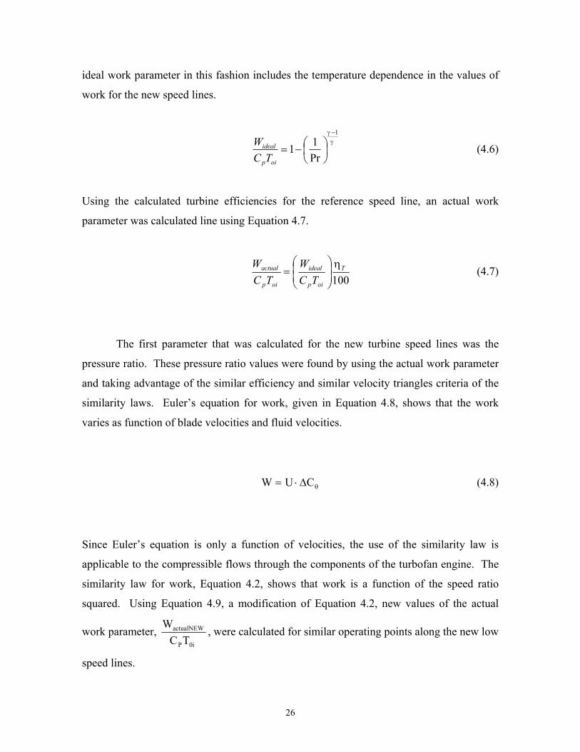
After these referred airflows and corrected torques were known for similar
operating points on the two percent-referred speed lines, these values were used to solve
for the exponents m and n in Equations 4.29 and 4.30.
m
REFRFRD
%50RFRD
REF
%50
N%N%
m
m
=
δθ
δθ
&
&
(4.29)
n
REFRFRD
%50RFRD
REF
%50
N%N%
q
q
=
δΤ
δΤ
(4.30)
Figure 4-5 shows three lines on a HP turbine corrected torque map. The two blue
lines are the lowest two speed lines from the normal operating speed map, 50% and 60%
referred speed. The red line is also a 50% referred speed line, however, it was constructed
using similar points to points on the reference speed line using Equation 4.30 with the
calculated exponent n. This was done to verify the quality of this exponent for
extrapolation showing that the lines for the two equal speeds were similar. This also
helped to show if some adjusting was needed.
These same exponents were then used in Equations 4.29 and 4.30 to extrapolate the
corrected torque and referred airflow parameters from idle to zero speed. The red lines
33

shown on Figure 4-6 are the extrapolated speed lines for corrected torque. The red lines
shown on Figure 4-7 are the extrapolated speed lines for referred airflow.
This characteristic map extrapolation method was performed for the LP turbine.
However, the method was not as successful with the LP turbine as with the HP turbine. It
was believed that the distance between the two lowest LP turbine speed lines was too great
to find an exponent value that would work well for stepping down in percent-referred
speed. From trial and error and by observing how the exponent affects the curves from the
HP turbine, exponents for the work, torque, and airflow similarity laws were slowly
changed until the curves appeared correct. This method was subjective, but was supported
by calculated LP turbine efficiencies not exceeding 100% efficiency.
These LP turbine exponents were used in Equations 4.9, 4.29, and 4.30 to
extrapolate the corrected torque and referred airflow parameters from idle to zero. The red
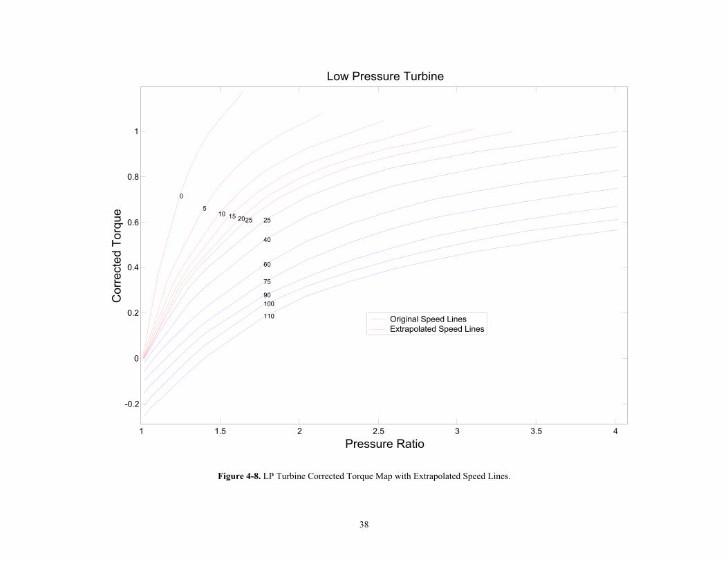
lines shown on Figure 4-8 are the extrapolated speed lines for corrected torque. The red
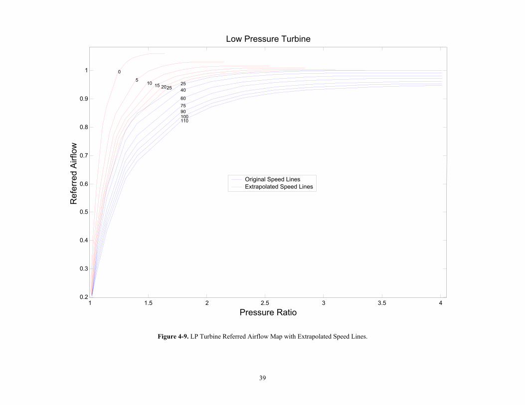
lines shown on Figure 4-9 are the extrapolated speed lines for referred airflow.
To this point in the extrapolation method, the efficiency values for the new speed
lines had been assumed the same as the reference speed line’s efficiency values. Since the
exponent had changed from the value from the similarity laws for the torque and mass flow
equations, the condition for similar efficiency was negated. New values of efficiency were
calculated for each of the new speed lines using their extrapolated parameters in Equation
4.5. Figures 4.10 and 4.11 show the new efficiency maps for the HP turbine and the LP
turbine respectively. Values and trends verify the correctness of the extrapolated
parameters.
Although these new turbine maps had speed lines of operation down to zero, the
maps were incomplete for use in the engine performance code. The computer simulation
required the model to provide map data in full and square matrices. In order to provide full
34

Figure 4-5. HP Turbine Corrected Torque Map with 50% & 60% map lines and 50% similar line.
10.2
High Pressure Turbine
Cor
rect
ed T
orqu
e
6 5.5 5 4.5 4 3.5 Pressure Ratio
3 2.5 2
0.3
0.4
0.5
0.6
0.7
0.8
50
Lowest Two Original Speed Lines Similar, Lowest Speed Line
50
60
1
0.9
1.5
35

Figure 4-6. HP Turbine Corrected Torque Map with Extrapolated Speed Lines.
Original Speed Lines Extrapolated Speed Lines
High Pressure Turbine
Cor
rect
ed T
orqu
e
10
15
20
25
30
35
40
45
50
100 105
90
80
70
60
50
1
0.9
0.8
0.7
0.6
0.5
0.4
0.3
0.2
0.1
6 5.5 5 4.5 4 3.5 Pressure Ratio
3 2.5 2 1.5 1 0 5
0
36

Figure 4-7. HP Turbine Referred Airflow Map with Extrapolated Speed Lines.
Original Speed Lines Extrapolated Speed Lines
High Pressure Turbine
Ref
erre
d Ai
rflow
0
5
10
15
20 25
30 35
40 45
50 105 100 90 80 70 60 50
0.95
0.9
0.85
0.8
0.75
5.5 5 4.5 4 3 3.5 Pressure Ratio
2.5 2 1.5 1
37
Original Speed Lines Extrapolated Speed Lines
Low Pressure Turbine
Cor
rect
ed T
orqu
e
0 5
10 220 15 5
110
90 100
75
60
40
25
1
0.8
0.6
0.4
0.2
0
-0.2
4 3.5 3 2.5 Pressure Ratio
2 1.5 1
Figure 4-8. LP Turbine Corrected Torque Map with Extrapolated Speed Lines.
38
Original Speed Lines Extrapolated Speed Lines
Low Pressure Turbine
Ref
erre
d Ai
rflow
0
5 10
220 15 5 25 40 60 75 90 100 110
1
0.9
0.8
0.7
0.6
0.5
0.4
0.3
4 3.5 3 2.5 Pressure Ratio
2 1.5 10.2
Figure 4-9. LP Turbine Referred Airflow Map with Extrapolated Speed Lines.
39

and square matrices each turbine speed line had to extend over the full range of pressure
ratios. However, having the full matrix maps caused the extension of some speed lines to
go into areas of their map where the engine would never operate. To extend all speed lines
to cover the full range of pressure ratios, a polynomial line fit was performed on every
speed line in each of the turbine maps. These polynomial fits were used to generate
complete maps for the HP turbine, shown in Figures 4-12 and 4-13, and LP turbine, shown
Figures 4-14 and 4-15, with speed lines that cover the full range of pressure ratios.
Though the turbine efficiency map were not a requirement for the model, it was
necessary to check that the maximum efficiency of each speed line never exceeded 100%.
With all speed lines extended to cover the full range of pressure ratios there was sufficient
information on both turbine maps to check all areas of the efficiency map. Figures 4-16
and 4-17 show the extended turbine efficiency for the HP and LP turbines respectively.
Having the plots of efficiency for the turbine as a check helped to verify the
extrapolated turbine parameters corrected torque and referred airflow were correct. There
were two things that were examined on the efficiency map to verify the turbine parameters.
First, that the turbine never exceeded 100% efficient, and second, that the efficiency lines
seemed consistent with efficiency maps discussed by Cohen et al. [2]. In the discussion by
Cohen et al. they stated that at low pressure ratios efficiency lines cross one another. For
both turbines, a spike of unreasonable efficiencies was located at the very lowest pressure
ratios. It was found that the referred airflow in the denominator of the efficiency
calculation was decreasing faster than the corrected torque and percent-referred speeds
were in the numerator. To compensate, the low end of the torque curves were adjusted
down enough to have the efficiency lines fall below 100%. The adjustment down in
turbine torque shows on Figure 4-13, the HP turbine corrected torque map, as an apparent
hole in the map between pressure ratios of 1.4 and 1.7. By adjusting the corrected torque
values rather than the referred airflow values, the efficiency lines shown in Figures 4-16
and 4-17 behaved more as Cohen, et al, had described. Additionally, smaller changes in
corrected torque were more influential on the efficiencies than adjusting the referred
airflow.
40

Figure 4-10. HP Turbine Efficiency Map with Extrapolated Speed Lines.
Original Speed Lines Extrapolated Speed Lines
High Pressure Turbine Ef
ficie
ncy
5
10
15
20
25
30
35
40 45
50
80 90 100 105
70
60
50
1
0.9
0.8
0.7
0.6
0.5
0.4
0.3
0.2
6 5.5 5 4.5 4 3.5 Pressure Ratio
3 2.5 2 1.5 10.1
0
41

Original Speed Lines Extrapolated Speed Lines
Low Pressure Turbine
Effic
ienc
y
0
5
10
15
20
110
60
75 90 100
40
25
1
0.9
0.8
0.7
0.6
0.5
0.4
0.3
0.2
0.1
4 3.5 3 2.5 Pressure Ratio
2 1.5 1 0
Figure 4-11. LP Turbine Efficiency Map with Extrapolated Speed Lines.
42

Figure 4-12. HP Turbine Referred Airflow Map with Extended Speed Lines.
1 1.5 2 2.5 3 3.5 4 4.5 5 5.50
0.1
0.2
0.3
0.4
0.5
0.6
0.7
0.8
0.9
1 0510152025
3035
4045
50
6070
80
90
100105
Pressure Ratio
Ref
erre
d A
irflo
wHigh Pressure Turbine
Percent Referred Speed Lines
43
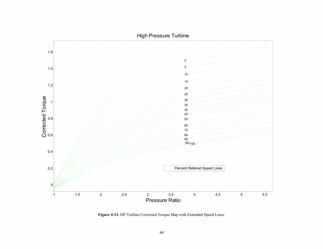
Figure 4-13. HP Turbine Corrected Torque Map with Extended Speed Lines.
1 1.5 2 2.5 3 3.5 4 4.5 5 5.5
0
0.2
0.4
0.6
0.8
1
1.2
1.4
1.6
0
5
10
15
20
25
3035404550
60708090100 105
Pressure Ratio
Cor
rect
ed T
orqu
eHigh Pressure Turbine
Percent Referred Speed Lines
44
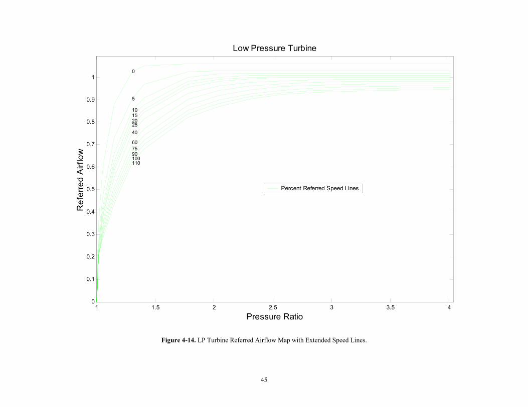
Figure 4-14. LP Turbine Referred Airflow Map with Extended Speed Lines.
1 1.5 2 2.5 3 3.5 40
0.1
0.2
0.3
0.4
0.5
0.6
0.7
0.8
0.9
10
5
1015202540
607590100110
Pressure Ratio
Ref
erre
d A
irflo
w
Low Pressure Turbine
Percent Referred Speed Lines
45

Figure 4-15. LP Turbine Corrected Map with Extended Speed Lines.
1 1.5 2 2.5 3 3.5 4
-0.2
0
0.2
0.4
0.6
0.8
1
1.2
0
5
10
1520
25
40
60
75
90100110
Pressure Ratio
Cor
rect
ed T
orqu
e
Low Pressure Turbine
Percent Referred Speed Lines
46

Figure 4-16. HP Turbine Efficiency Map with Extended Speed Lines.
1.5 2 2.5 3 3.5 4 4.5 5 5.5
0
0.2
0.4
0.6
0.8
1
1.2
0
5
10
15
20
25
30
35404550
60708090
100105
Pressure Ratio
Effi
cien
cy
High Pressure Turbine
Percent Referred Speed Lines
47

Figure 4-17. LP Turbine Efficiency Map with Extended Speed Lines.
1 1.5 2 2.5 3 3.5 40
0.1
0.2
0.3
0.4
0.5
0.6
0.7
0.8
0.9
1
0
5
10
15
20
25
40
6075
90100
110
Pressure Ratio
Effi
cien
cyLow Pressure Turbine
Percent Referred Speed Lines
48

Fan and Compressor Maps. The compressor characteristics for the engine simulation
were defined using three beta maps. The first beta map contained referred airflow as a
function of percent-referred speed for constant beta lines. The second beta map contained
pressure ratio as a function of percent-referred speed for constant beta lines. The third beta
map contained efficiency as a function of percent-referred speed for constant beta lines.
These three beta maps were converted into two conventional map formats. One of these
maps shows pressure ratio as a function of referred airflow, δ
θm& , with lines constant of
percent-referred speed. The other of these maps shows efficiency as a function of referred
airflow, δ
θm& , with lines constant of percent-referred speed.
The extrapolation method for the fan and compressors began by using the same
principles as for the turbines. The reference line selected was the lowest percent-referred
speed line on the map. First, the ideal work parameter along the reference speed line was
calculated using the compressor work equation, Equation 4.31.
( ) γγ 1
Pr1−
−= REFoip
idealREFC
TCW
(4.31)
Then the actual work parameter along the reference speed line was calculated using
Equation 4.32 and compressor efficiency.
REFCoip
idealREFC
oip
actualREFC
TCW
TCW
η100
= (4.32)
49

The work similarity law was used to extrapolate the actual work parameter to the new
speed lines using Equation 4.33.
2
%%
=
REFRFRD
NEWRFRD
oip
actualREFC
oip
actualNEWC
NN
TCW
TCW
(4.33)
The pressure ratios along the extrapolated speed lines were calculated using Equation 4.34.
1
1001Pr
−
−=
γγ
η REFC
oip
actualNEWCNEW TC
W (4.34)
It was found using the incompressible exponent (exponent equal to 1) for the airflow
similarity laws gave good results when extrapolating the fan and compressors' referred
airflow into the low speed region. The mass flow relationship is Equation 4.35.
=
δθ
δθ
REFRFRD
NEWRFRD
REF
NEW
N%N%
m
m
&
&
(4.35)
Using these extrapolated pressure ratio and referred airflow values, new pressure
ratio maps for the fan and compressors were developed as shown in Figures 4.18 through
4.21. The fan and compressors’ figures show the original map speed lines in blue,
extrapolated speed lines in red, and the surge line in green. Figures 4-18 and 4-19 are the
characteristic maps for the fan. Figures 4-18 shows fan hub (or core flow) pressure ratio as
50

a function of referred fan airflow for the entire frontal area of the fan, used for all maps, for
lines of constant percent-referred speed. Figures 4-19 shows fan tip (or by-pass flow)
pressure ratio as a function of referred fan airflow for lines of constant percent-referred
speed. However, since all of the core flow travels through the compressors, it was only
necessary to have one characteristic map for the compressors. For the fan, the flow is
divided in two parts, hub and tip. Figures 4-20 shows the characteristic map for the LP
compressor and Figures 4-21 show the characteristic map for the HP compressor. The
compressors, LP and HP, have similar maps to the fan in regard to their layout; referred
airflow as a function of pressure ratio for lines of constant percent-referred speed.
Using the mass flow and work similarity laws satisfied the criteria for constant
efficiencies. In general for fans and compressors, efficiency decreases as speed decreases.
To account for changing efficiencies for the components in this model, without losing the
quality low speed referred airflow and pressure ratio characteristics, the exponent of a
torque similarity law was changed. The next step for these components was to calculate
corrected torque along the reference speed line. The reference rotational speed in RPM
was calculated using Equation 4.36.
100% θ
θMAX
RFRDREFN
NNREF
⋅= (4.36)
The mass flow rate was calculated along the reference speed line using Equation 4.37.
θδ
δθ
⋅= REFREF
mm
&& (4.37)
51

Figure 4-18. Fan Hub (Core) Pressure Ratio map with Extrapolated Speed Lines.
Original Map Speed Lines Extrapolated Speed Lines
Fan
Hub
Pre
ssur
e R
atio
0 10
115
110
105
100
95
90
85
80
70
60
45
17.5
1.8
1.7
1.6
1.5
1.4
1.3
1.2
1.1
1 0.9 0.8 0.7 0.4 0.5 0.6 Referred Airflow
0.3 0.2 0.1 01
52

Figure 4-19. Fan Tip (Bypass) Pressure Ratio map with Extrapolated Speed Lines.
Original Map Speed Lines Extrapolated Speed Lines
Fan
Tip
Pres
sure
Rat
io
0 10
115
110
105
100
95
90
85
80
70
60
45
17.5
1.9
1.8
1.7
1.6
1.5
1.4
1.3
1.2
1.1
1 0.9 0.8 0.7 0.6 0.4 0.5 Referred Airflow
0.3 0.2 0.1 0 1
53

Original Map Speed Lines Extrapolated Speed Lines Surge Line
Low Pressure Compressor
Pres
sure
Rat
io
0 10 20 30
40
110 105
100
95
90
85
80
75
70
60
50
6
5.5
5
4.5
4
3.5
3
2.5
2
1.5
1 0.9 0.8 0.7 0.4 0.5 0.6 Referred Airflow
0.3 0.2 0.1 0 1
Figure 4-20. Low Pressure Compressor Pressure Ratio map with Extrapolated Speed Lines.
54

Original Map Speed Lines Extrapolated Speed Lines Surge Line
High Pressure Compressor
Pres
sure
Rat
io
0 10 20 30
40
50
108
103.9713
100 96.9032
93.128
89.4736
85.5432
81.4999
77.1562
68.3232
58.388
3
2.5
2
1.5
1 1 0.9 0.8 0.7 0.5 0.6
Referred Airflow 0.4 0.3 0.2 0.1 0
Figure 4-21. High Pressure Compressor Pressure Ratio map with Extrapolated Speed Lines.
55

Power was solved along the reference speed line because torque was needed.
Power was the logical choice because it could be calculated from the pressure ratio, the
mass flow rate, and the efficiency using Equation 4.38.
γ−γ
η
=1
REFoiREFC
PREFREF PrT100CmPwr & (4.38)
The corrected torque was calculated along the reference speed line using Equation 4.39.
REF
REFREF
N2wrq
πδΡ
=δ
Τ (4.39)
After values of corrected torque along the reference line were found, the similarity
law for power, which has a cubic power speed ratio, was reduced to find a similarity law
for torque. It was found that the speed ratio for a torque similarity law would need to be
squared. Again if this exponent were used, the efficiencies would have remained the same
as the reference values. However, by varying the exponent n used in the torque similarity
law, Equation 4.40, different efficiencies for the extrapolated lines were calculated.
n
REFRFRD
NEWRFRDREFNEW
N%N%qq
δ
Τ=
δΤ
where, n = 1.75 (4.40)
The fan and compressor efficiencies were calculated using Equation 4.41.
56

δΤ
⋅⋅θ
⋅π
−⋅⋅
δθ
=ηγ−γ
NEWNEW
1
NEWambPNEW
C qmaxN
N2
1PrTCm&
(4.41)
The efficiency maps generated show that these component characteristic maps are
in agreement with the engine manufacturer’s efficiency extrapolation method [11]. It is
important to note that a criteria for the efficiency extrapolation method was that the peaks
of each of the efficiency curve form a ‘backbone’ shape. The exponent for the torque
similarity law was adjusted until the efficiency curves formed the ‘backbone’ as shown in
Figures 4.22 through 4.25. The maps show that the calculated efficiencies fall to low
efficiencies at the low percent–referred speeds [12]. Figure 4-22 shows fan tip efficiency
as a function of referred fan airflow for lines of constant percent-referred speed. Figure 4-
23 shows fan hub efficiency as a function of referred fan airflow for lines of constant
percent-referred speed. The LP and HP compressor efficiencies are shown in Figures 4-24
and 4-25 respectively.
Most of the lowest extrapolated lines had to be extended to cover the area of
starting operation. Therefore, these lines were individually extended over a wider range of
pressure ratios to cover their area of starting operation. It was necessary to assume some
special operating conditions when the zero speed line was extended. Figure 4-26, a figure
from Walsh and Fletcher’s [1] discussion on starting dynamics, details these operating
conditions nicely. When a component is not rotating and there is no flow through the
component it has a pressure ratio equal to one. However, it is possible to have flow
through a stationary component, such as the fan prior to the low-speed shaft breaking its
seals and bearing static friction. When this happens there is a pressure drop across the
component, thus a pressure ratio less than one.
57

Original Speed Lines Extrapolated Speed Lines
Fan
Hub
Effi
cien
cy
0
10
110 115
105 100
95 90 85 80 70 60
45
17.5
1
0.9
0.8
0.7
0.6
0.5
0.4
1 0.9 0.8 0.7 0.4 0.5 0.6 Referred Airflow
0.3 0.2 0.1 0 0.3
Figure 4-22. Fan Hub (Core) Efficiency map with Extrapolated Speed Lines.
58

Original Speed Lines Extrapolated Speed Lines
Fan
Tip
Effic
ienc
y
0
10
110 115
105 100 95 90 85 80 70
60
45
17.5
1
0.9
0.8
0.7
0.6
0.5
0.4
0.3
1 0.9 0.8 0.7 0.4 0.5 0.6 Referred Airflow
0.3 0.2 0.1 00.2
Figure 4-23. Fan Tip (Bypass) Efficiency map with Extrapolated Speed Lines.
59

Original Speed Lines Extrapolated Speed Lines
Low Pressure Compressor
Effic
ienc
y
10
20
30
40
110 105
100 95 90 85
80
75 70
60
50
1
0.9
0.8
0.7
0.6
0.5
0.4
0.3 0
1 0.9 0.8 0.7 0.4 0.5 0.6 Referred Airflow
0.3 0.2 0.1 00.2
Figure 4-24. Low Pressure Compressor Efficiency map with Extrapolated Speed Lines.
60

Original Speed Lines Extrapolated Speed Lines
High Pressure Compressor
Effic
ienc
y 10
20
30
40
50
97 100 104 108
93 89 86 81 77 68 58
1
0.9
0.8
0.7
0.6
0.5
0.4
0.3 0
0.2
0.1
1 0.9 0.8 0.7 0.4 0.5 0.6 Referred Airflow
0.3 0.2 0.1 00
Figure 4-25. High Pressure Compressor Efficiency map with Extrapolated Speed Lines.
61

Figure 4-26. Demonstration of zero speed, flow greater than zero, and pressure ratio less than one.
When extending the zero percent referred speed line, these flow conditions were
accounted for on the fan and compressor maps. Figures 4-27 through 4-30 are the fan and
compressor maps showing the poly-fitted extended low speed lines.
62

Percent Referred Speed Lines Surge Line
Fan
Hub
Pre
ssur
e R
atio
0 10
115
110
105
100
95
90
85
80
70
60
45
17.5
1.7
1.6
1.5
1.4
1.3
1.2
1.1
1
1 0.9 0.8 0.7 0.4 0.5 0.6 Referred Airflow
0.3 0.2 0.1 0
Figure 4-27. Fan Hub (Core) Pressure Ratio map with Extended Speed Lines.
63

Percent Referred Speed Lines Surge Line
Fan
Tip
Pres
sure
Rat
io
0 10
115
110
105
100
95
90
85
80
70
60
45
17.5
1.9
1.8
1.7
1.6
1.5
1.4
1.3
1.2
1.1
1
0.9
1 0.9 0.8 0.7 0.6 0.4 0.5 Referred Airflow
0.3 0.2 0.1 0
Figure 4-28. Fan Tip (Bypass) Pressure Ratio map with Extended Speed Lines.
64

Figure 4-29. Low Pressure Compressor Pressure Ratio map with Extended Speed Lines.
Percent Referred Speed Lines Surge Line
Low Pressure Compressor
Pres
sure
Rat
io
0 10 20 30
40
110 105
100
95
90
85
80
75
70
60
50
6
5
4
3
2
1
1 0.9 0.8 0.7 0.4 0.5 0.6 Referred Airflow
0.3 0.2 0.1 0
65

Figure 4-30. High Pressure Compressor Pressure Ratio map with Extended Speed Lines.
Percent Referred Speed Lines Surge Line
High Pressure Compressor
Pres
sure
Rat
io
0 10 20 30
40
50
108
103.9713
100 96.9032
93.128
89.4736
85.5432 81.4999
77.1562
68.3232
58.388
3
2.5
2
1.5
1
1 0.9 0.8 0.7 0.5 0.6 Referred Airflow
0.4 0.3 0.2 0.1 0
66

CHAPTER 5
Comparison of Simulated Starting Results
with Experimental Data
The engine simulation program was used to predict the turbofan engine starting
operation using the extrapolated low speed characteristics from combustor ignition speed
through idle speed. When the simulation was completed, the predicted values were
compared against experimentally measured data from two sources. The comparison of the
simulated starting results with experimentally measured data is discussed in this chapter.
There is limited experimental data available for gas turbine engines during starting.
For the turbofan engine studied in this work two sets of starting data were obtained from
independent sources. One set of data was from the engine manufacturer's initial engine
trial tests. Although initial engine testing is primarily for normal engine operations and
meeting contract specifications, some engine starting tests are usually done. The second
set of experimental starting data was run by the United States Air Force Academy at the
request of this researcher. One of the Air Force Academy's test cells contains a fully
automated and instrumented turbofan engine; the same turbofan engine modeled in this
research. Despite different starting procedures, techniques, and initial conditions, it was
found that these two sets of test data showed similar engine pressures, temperatures, and
speed through 20,000 RPM of the high-speed shaft. Both sources ended the collection of
starting data at this speed. For this turbofan engine, 20,000 RPM is near idle speed,
~23,000 RPM. Above idle speed, the starter motor was disengaged and the pressures were
sufficient to close the surge value.
The engine manufacturer's turbofan performance model was written to match
normal operating speeds, idle to full power, and did not allow for simulation without
combustion. Therefore, the speeds used in the current engine starting simulation were
from ignition speed, 10,000 RPM, to idle speed. The parameters that were to be compared
67

to the experimental starting data were easily accessible from the simulation model.
Figures 5-1 through 5-4 shows the selected experimental starting data from zero to 20,000
RPM. On the figures, the engine manufacturer's data is shown in black and the Air Force
Academy data in blue. The values of these parameters, as predicted by the engine
simulation for values for speeds from 10,400 RPM through 20,000 RPM, are shown with
green stars. The red vertical line on these figures marks the ignition speed at 10,000 RPM.
These figures were produced using a script file written in MatLab5.3SE (The MathWorks,
Inc.). The script file name is in Appendix B.
Figure 5-1 shows the stations where the experimentally measured data was taken
on a schematic of the turbofan engine modeled in this research. Station 3 is the HP
compressor discharge, station 41 is the HP turbine inlet, and station 45 is intermediate
turbine.
FAN LP
C
HPC
HPT
LPT
3 41 45
Combustor
FAN LP
C
HPC
HPT
LPT
3 41 45
Combustor
Figure 5-1. Schematic of the turbofan engine modeled for starting research.
Figure 5-2 shows the HP compressor discharge static pressure, PS3, as a function of
percent of design high-speed shaft speed. Figure 5-3 shows HP compressor discharge total
pressure, PT3, as a function of percent of design high-speed shaft speed. The predicted
pressure at the HP compressor discharge was an important parameter to compare the
experimental data. If these pressures had not compared favorably it would have been an
indication of problems with the fan and compressors' pressure ratio characteristics. The
fact that the static and total pressures did compare favorably, indicates that the extrapolated
pressure ratio characteristics matched well for the fan and compressor working together.
68

Figure 5-2. PS3/Pamb as a function of percent of design high speed.
0 5 10 15 20 25 30 35 40 452
2.2
2.4
2.6
2.8
3
P e rce nt o f D e sig n H ig h-sp e e d S haft S p e e d
Ps3/P
amb
M anufacturers D ata Ignition S peed S im ulation P redictions
69

Figure 5-3. PT3/Pamb as a function of percent of design high speed shaft.
0 5 10 15 20 25 30 35 40 45 50
2
2.2
2.4
2.6
2.8
3
P e rce nt o f D e sig n H ig h-sp e e d S haft S p e e d
Pt3/P
amb
A cadem y A cadem y D ata Ignition S peed S im ulation P redictions
70

The next engine parameter that was compared was the intermediate turbine
temperature, T45. Figure 5-4 shows non-dimensional temperature, θ45, as a function of
percent of design high-speed shaft speed. Turbine temperature was another important
parameter for comparison because it showed that the mass flow, pressures, and
temperatures prior to the turbines were being accurately calculated from the extrapolated
areas of the component characteristic maps. It can be seen on Figure 5-4 that up to about
37% of design high- speed shaft speed the simulation did well in predicting θ45, however,
above that speed the temperatures begin to deviate from the engine manufacturer’s data.
Some experimenting with the simulation in an effort to eliminate this difference showed
that a steady state T45 at the higher temperatures would not converge because turbine inlet
temperature, T41, would exceed turbine material temperature limits set in the model. It is
believed that the higher temperatures in the experimental data are a result of transient
effects. That is, the experimental data shows the higher temperature as the engine settles
from the starting acceleration to a constant idle speed. The higher temperatures are not
predicted with a quasi-steady analysis. Some of the influences that may exacerbate the
higher temperature could be a result of the control of the throttle or the response of fuel
management program. Other than not predicting the higher temperature, the low-speed
simulation did well in matching the experimental data for the intermediate turbine
temperature. This indicates that the extrapolated turbine maps adequately predict turbine
performance.
The last simulated parameter selected for comparison with the experimental data
was percent of design low-speed shaft speed as a function of percent of design high-speed
shaft speed. Each engine and starting cycle will have its own unique path of acceleration.
It can be seen in Figure 5-5 that low-speed shaft can break its seal and bearing static
friction and begin to rotate at different times depending on the acceleration of high-speed
shaft. Although, the low-speed shaft in the two sets of experimental data clearly begin to
rotate at different speeds of the high-speed shaft, they end up at the same speed at engine
idle. The steady state simulation predicted similar values and trends from ignition to idle
when compared to the two sets of experimental data. However, the early predictions of
low-speed shaft speed were considerably higher than those presented here. An
71

0 5 10 15 20 25 30 35 40 45 501
1.5
2
2.5
3
3.5
4
P e rce nt o f D e sig n H ig h-sp e e d S haft S p e e d
T45/T
amb
M anufacturers D ata Ignition S peed S im ulation P redictionsA ir F orce A cadem y D ata
Figure 5-4. θ45 as a function of percent of design high speed shaft.
72

investigation led to the fan, a component on the low-speed shaft. After some investigation
by changing speed line values and observing the effects, it was determined that the lowest
known percent-referred speed line value (20%) on the manufacturer's map was actually
2.5% too high. This difference was over predicting the characteristics for the extrapolated
10% referred speed line. Lowering the 20% referred speed line to a value of 17.5%
brought the characteristics for the 10% referred speed line up. Without major effect on
other engine parameters, the change in the fan percent-referred speed line dropped the
predicted low-speed shaft speeds closer to the experimental data. With these changes, the
simulation was predicting selected engine parameters with reasonable accuracy. The
simulated engine equilibrium running line was then drawn on the fan and LP compressor
characteristic maps.
73

Figure 5-5. Design low speed shaft as a function of percent of design high speed shaft.
0 5 10 15 20 25 30 35 40 45 500
2
4
6
8
10
12
14
16
18
20
P e rce nt o f D e sig n H ig h-sp e e d S haft S p e e d
Percent of Design Low-speed S
haft S
peed
M anufacturers D ata Ignition S peed S im ulation P redictionsA ir F orce A cadem y D ata
74

CHAPTER 6
Surge Valve Variable Area Results
The objective of this research was to find a surge valve schedule that would
decrease the turbine inlet temperature as the engine comes up in speed, while maintaining
an adequate stall margin. Once it was shown that the engine simulation, using the
extrapolated characteristic maps, adequately predicted engine performance, the effect of
varying the surge valve area was investigated.
The first step in this investigation was to determine the engine equilibrium running
line with the fixed area surge valve (0.26 in2) currently installed in the engine. Figures 6-1
and 6-2 show the engine equilibrium running line on the characteristic maps for the fan tip
and hub, respectively. Figures 6-3 shows the engine equilibrium running line on the
characteristic map for the LP compressor.
6.1 Equilibrium Running Lines for Varying Valve Area
The equilibrium running lines for the fixed 0.26 in2 surge valve area, shown in
Figures 6-1 through 6-3, were then compared to additional engine equilibrium running
lines where the surge valve bleed area was changed. Figures 6-4 shows the engine
equilibrium running lines on the characteristic map for the LP compressors. This figure
shows the effects of changing the surge valve bleed area on the engine equilibrium running
lines. The equilibrium running lines shown on Figure 6-4 are for valve areas of 0.0 in2
(closed valve), 0.12 in2, 0.26 in2, and 0.4 in2. The equilibrium running line closest to the
surge line is for a valve area of 0.0 in2 and as the valve area increases in size, the
equilibrium running lines move down and away from the surge line.
75

Much of what is found in the literature concerning starting behavior can be seen in
the equilibrium running lines developed from the computer simulations. In particular,
Wilson’s [4] discussion of surge valve use to increase stall margin is clearly evident on the
LP compressor characteristic map. As the valve area, and thus the bleed flow, was
increased the equilibrium running lines moved to lower pressure ratios and away from the
surge line.
76

77
Figure 6-1. Fan Hub Pressure Ratio map with 0.26in2 Valve Area Equilibrium running line.
Fan
115
110
1.7 105
100 1.6
95
90 1.5
Hub
Pre
ssur
e R
atio
85
1.4 80
70 1.3
60 1.2
45 1.1
Percent Referred Speed Lines Surge Line Equilibrium Running Line
17.5 10
1 0
0 0.1 0.2 0.3 0.4 0.5 0.6 Referred Airflow
0.7 0.8 0.9 1

Figure 6-2. Fan Tip Pressure Ratio map with 0.26in2 Valve Area Equilibrium running line.
Percent Referred Speed Lines Surge Line Equilibrium Running Line
Fan
Tip
Pres
sure
Rat
io
10
115
110
105
100
95
90
85
80
70
60
45
17.5
1.9
1.8
1.7
1.6
1.5
1.4
1.3
1.2
1.1
1 0
1 0.9 0.8 0.7 0.4 0.5 0.6 Referred Airflow
0.3 0.2 0.1 0
78

Figure 6-3. Low Pressure Compressor Pressure Ratio map with 0.26in2 Valve Area Equilibrium running line.
Percent Referred Speed Lines Surge Line Equilibrium Running Line
Low Pressure Compressor
Pres
sure
Rat
io
10 20 30
40
110 105
100
95
90
85
80
75
70
60
50
6
5.5
5
4.5
4
3.5
3
2.5
2
1.5
1 0
1 0.9 0.8 0.7 0.4 0.5 0.6 Referred Airflow
0.3 0.2 0.1 0
79

Percent Referred Speed Lines Surge Line Equilibrium Running Lines
Low Pressure Compressor
Pres
sure
Rat
io
10 20 30
40
110 105
100
95
90
85
80
75
70
60
50
6
5
4
3
2
1 0
1 0.9 0.8 0.7 0.4 0.5 0.6 Referred Airflow
0.3 0.2 0.1 0
Figure 6-4. Low Pressure Compressor Pressure Ratio map with various Valve Area Equilibrium running lines.
80

6.2 Parametric Study of Varying Valve Area
In this simulation the bleed conditions, that is, temperature, pressure, and flow were
all calculated values. In order to change the bleed conditions, without major modification
to the model, was to simply change the bleed flow area. Changing the valve flow area for
each simulation created a family of curves for each predicted engine parameter. Figures 6-
5 through 6-9, show selected engine parameters as a function of surge valve bleed area and
percent design of high-speed shaft speed. A script file was written for MatLab5.3SE (The
MathWorks, Inc.) to plot the three-dimensional plots of the simulation's predictions for
various surge valve bleed areas. See Appendix B for the script file name.
During starting, the LP compressor surge margin is much smaller than the surge
margin of the HP compressor. Therefore, in this study the LP compressor surge margin
was used as the criteria for satisfactory engine performance. Surge margin was defined as
the percent difference between the pressure ratio at the surge line and the engine
equilibrium running line. As shown in Figure 6-5, as the surge valve area decreases the
surge margin approaches zero.
It was demonstrated in Chapter 5 that the simulation adequately predicted the
intermediate turbine temperature, T45. Temperature, T45, was selected for comparison
because of the very high temperatures and inaccessibility of the turbine inlet prevented the
measurement of the turbine inlet temperature, T41. Non-dimensional turbine inlet
temperature, θ41, as shown in Figure 6-6, was selected for the simulation study here
because it is more critical to engine performance. As shown in Figure 6-6 the turbine inlet
temperature decreases as the surge valve flow area is decreased. This is due to the
increased airflow through the engine core as the bypass airflow is reduced.
Figure 6-7 and 6-8 show the power required by the LP and HP compressors,
respectively. As seen in Figure 6-7, the power required by the LP compressor is reduced
as the surge valve flow area is decreased. Figure 6-8 shows that the HP compressor's
81

0
0.1
0.2
0.3
0.4
2025
3035
4045
50
-5
0
5
10
15
20
25
V alve A re a [inch2 ]
P e rce nt o f D e sig n H ig h-sp e e d S haft S p e e d
LPC S
urg
e M
arg
in [%
]
S urge V alve F ixed A rea
Figure 6-5. Low Pressure Compressor Surge Margin as a function of percent of design high-speed shaft speed and valve area.
82

Figure 6-6. θ41 as a function of percent of design high-speed shaft speed and valve area.
0
0.05
0.1
0.15
0.2
0.25
0.3
0.35
0.4
2025
3035
4045
50
1.6
1.8
2
2.2
2.4
2.6
2.8
3
3.2
3.4
3.6
V alve A re a [inch2 ]P e rce nt o f D e sig n H ig h-sp e e d S haft S p e e d
T41/T
amb
S urge V alve F ixed A rea
83

required power is also decreased as the surge valve flow area is decreased, although to a
lesser degree. Thus, the required power of the overall compressor section is reduced. This
reduced power means that the power and torque supplied by the HP turbine and/or starter
motor is reduced.
Additional engine parameters, such as PS3, PT3, and low-speed shaft speed were
also predicted in the simulation but not shown here, because they were not strongly
dependent on surge valve bleed area.
6.3 Surge Valve Area Schedule
The next step in this study was to select a surge valve area schedule that would maintain a
minimum adequate surge margin and thus maintain minimum turbine inlet temperatures.
The parametric study results discussed in the previous section were used to determine the
surge valve flow area as a function of percent of design high-speed shaft speed to meet this
goal. While this analysis could be done for any selected surge margin it was decided that a
minimum surge margin of 6% would be used. This is the minimum value that occurred
using the manufacturer's constant surge valve flow area of 0.26 in2. In Figure 6-9, the red
line superimposed on the parametric plot of the LP compressor surge margin shows the
locus of points that provide a minimum surge margin of 6% between approximately 30%
and 45% of design high-speed shaft speed. It was found that below approximately 30% of
design high-speed shaft speed, a minimum flow area of 0.26 in2 was required in order to
obtain a turbine/compressor match. It is believed that this is due to the fact that at these the
low pressure compressor is stalled. While it may be feasible to accelerate through this area
with the compressor stalled, it was decided for the purposes of this study to select surge
valve flow areas that would ensure that the low pressure compressor never stalled. Above
approximately 45% of design high-speed shaft speed the surge valve was completely
closed and surge margin continued to increase. Figure 6-10 shows this surge valve flow
area as a function of percent of design high-speed shaft speed.
84

Figure 6-7. Low Pressure Compressor Power of percent of design high-speed shaft speed and valve area.
0
0.05
0.1
0.15
0.2
0.25
0.3
0.35
0.4
2025
3035
4045
50
0
10
20
30
40
50
60
V alve A re a [inch2 ]P e rce nt o f D e sig n H ig h-sp e e d S haft S p e e d
LPC P
ower [hp]
S urge V alve F ixed A rea
85

0
0.05
0.1
0.15
0.2
0.25
0.3
0.35
0.4
2025
3035
4045
50
5
10
15
20
25
30
35
V alve A re a [inch2 ]P e rce nt o f D e sig n H ig h-sp e e d S haft S p e e d
HPC P
ower [hp]
S urge V alve F ixed A rea
Figure 6-8. High Pressure Compressor Power of percent of design high-speed shaft speed and valve area.
86

Figure 6-9. Variable valve schedule surge margin superimposed on the parametric plot of the LP compressor surge margin.
0
0.05
0.1
0.15
0.2
0.25
0.3
0.35
0.4
2025
3035
4045
50
-5
0
5
10
15
20
25
V alve A re a [inch2 ]P e rce nt o f D e sig n H ig h-sp e e d S haft S p e e d
LPC S
urg
e M
arg
in [%
]
S urge V alve V arible A reaS urge V alve F ixed A rea
87
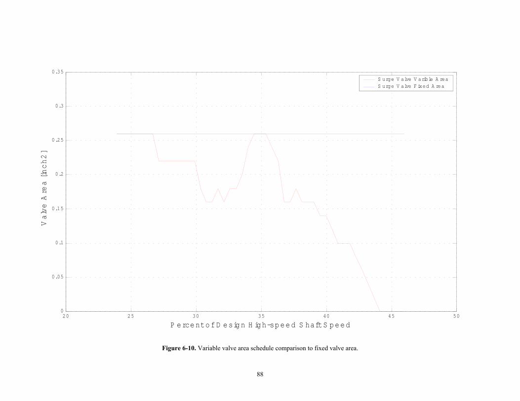
Figure 6-10. Variable valve area schedule comparison to fixed valve area.
20 25 30 35 40 45 500
0.05
0.1
0.15
0.2
0.25
0.3
0.35
P e rce nt o f D e sig n H ig h-sp e e d S haft S p e e d
Valve A
rea [inch2]
S urge V alve V arible A reaS urge V alve F ixed A rea
88

Figure 6-11 shows a comparison of the current fixed area valve surge margin (blue
line) and the new variable surge valve flow area surge margin (red line).
Figure 6-12 shows the locus of turbine inlet temperatures that would result by
maintaining a minimum surge margin of 6% superimposed on the parametric plot of the
turbine inlet temperature. Figure 6-13 shows a comparison of the current fixed area valve
turbine inlet temperature (blue line) and the new variable surge valve flow area turbine
inlet temperature (red line). The variable surge valve flow area schedule produces a lower
turbine inlet temperature over the entire speed range with two exceptions. These are in the
low speed range, where the 0.26 in2 area was used, and at approximately 35% of design
high-speed shaft speed where the variable and fixed areas both provided minimum surge
margin. The nearly fifty degree reduction in turbine inlet temperature at approximately
45% of design high-speed shaft speed is a result of the surge valve being fully closed when
using the variable surge valve flow area schedule.
Figure 6-14 shows a comparison of the current fixed area valve LP compressor
power (blue line) and the new variable surge valve flow area LP compressor power (red
line). The variable surge valve flow area schedule produces a lower LP compressor power
over the entire speed range with two exceptions. These are in the low speed range, where
the 0.26 in2 area was used, and at approximately 35% of design high-speed shaft speed
where the variable and fixed areas both provided minimum surge margin. The nearly five
horsepower reduction in turbine inlet temperature at approximately 45% of design high-
speed shaft speed is a result of the surge valve being fully closed when using the variable
surge valve flow area schedule.
Parameters such as turbine inlet temperature and LP compressor power could be
further reduced if a smaller surge margin was deemed feasible.
89

Figure 6-11. Variable valve area schedule surge margin comparison to fixed valve area surge margin.
20 25 30 35 40 45 505
10
15
20
LPC S
urg
e M
arg
in [%
]
P e rce nt o f D e sig n H ig h-sp e e d S haft S p e e d
S urge V alve V arible A reaS urge V alve F ixed A rea
90

Figure 6-12. Variable valve schedule θ41 superimposed on the parametric plot of θ41.
0
0.05
0.1
0.15
0.2
0.25
0.3
0.35
0.4
2025
3035
4045
50
1.6
1.8
2
2.2
2.4
2.6
2.8
3
3.2
3.4
3.6
V alve A re a [inch2 ]P e rce nt o f D e sig n H ig h-sp e e d S haft S p e e d
T41/T
amb
S urge V alve V arible A reaS urge V alve F ixed A rea
91

20 25 30 35 40 45 501.6
1.8
2
2.2
2.4
2.6
2.8
3
3.2
3.4
3.6
T41/T
amb
P e rce nt o f D e sig n H ig h-sp e e d S haft S p e e d
S urge V alve V arible A reaS urge V alve F ixed A rea
Figure 6-13. Variable valve area schedule θ41 comparison to fixed valve area θ41.
92

20 25 30 35 40 45 505
10
15
20
25
30
35
40
45
50
55LPC P
ower [hp]
P e rce nt of D esign H igh-speed S haft S peed
S urge V alve V arible A reaS urge V alve F ixed A rea
Figure 6-14. Variable valve area schedule LP compressor power comparison to fixed valve area LP compressor power.
93

Chapter 7
Conclusions
A new method for extrapolating low speed, low flow characteristics was developed
in this research. The method used conventional component characteristic map formats to
extrapolate the low speed, low flow characteristics. Using selected reference lines, new
exponents for the incompressible similarity laws incorporated compressibility effects based
on thermodynamic and fluid mechanic properties. The exponents remained the same for
extrapolating their respective parameters. The new low speed, low flow characteristics,
were used to calculate efficiencies and verify that efficiencies remained below 100%. The
extrapolation method for an axial fan, a centrifugal compressor, and an axial turbine
developed new characteristic speed lines with good agreement with the physical operation
of the turbofan engine components.
A simulation using the extrapolated component characteristics showed that the
steady-state equilibrium predictions matched reasonably well to measured starting data.
The simulations preformed in the parametric study show that, indeed, the use of a surge
valve variable flow area schedule could result in reduced turbine inlet temperatures during
the start-up process. This can be accomplished while maintaining a minimum adequate
surge margin. In addition, another beneficial result is a reduction in starting torque.
94

Chapter 8
Recommendations
The results and experience gained during this investigation suggest several areas
for additional study. The following are considered to be especially pertinent:
(1) Improve the model to include the dynamics of the rotors' inertia. This will
allow the simulation to include the effect on the surge margin due to
transient effects.
(2) Improve the model to simulate the pre-ignition conditions.
(3) Investigate compressor performance in the stall region. Currently, engine
simulations fail in the undefined regions of a stalled compressor map.
(4) Measure the low speed/low flow characteristic of fans, compressors and
turbines. This experimental data would provide a better basis for the
simulation of the engine start-up process.
95

References
[1] Walsh, P. P., and P. Fletcher, Gas Turbine Performance (Fairfield: Blackwell Science Ltd. And ASME, 1998). [2] Cohen, H., G. F. C. Rogers, and H. I. H. Saravanamuttoo, Gas Turbine Theory 2nd ed. (London: Longman Group Limited, 1972). [3] Aungier, R. H., Centrifugal Compressors: A Strategy for Aerodynamic Design and Analysis (New York: The American Society of Mechanical Engineers, 2000). [4] Wilson, D. G., The Design of High-Efficiency Turbomachinery and Gas Turbines (Cambridge: The MIT Press, 1984). [5] Hill, P. and C. Peterson, Mechanics and Thermodynamic of Propulsion 2nd ed. (Reading: Addison-Wesley Publishing Company, 1992). [6] Wilkes, K., and W. F. O’Brien, “Dynamic Modeling of Starting Aerodynamic and Stage Matching in an Axial-Centrifugal Compressor,” ASME 96-GT-278. [7] Agrawal, R. K., and M. Yunis, “A Generalized Mathematical Model to Estimate Gas Turbine Starting Characteristics,” Transactions of the ASME, vol. 104 (Jan. 1982), pp. 194-201. [8] Kurzke, J., “How to Get Component Maps for Aircraft Gas Turbine Performance Calculations,” ASME 96-GT-164 (1996). [9] TFE109-1 Turbofan Engine Installation Manual, Allied-Signal (Dec. 1992). [10] Munson, B. R., D. F. Young, and T. H. Okiishi, Fundamentals of Fluid Mechanics 3rd ed. update (New York: John Wiley & Sons, Inc., 1998). [11] Private discussion with M. Sandifur, Honeywell Corp. Performance and Operability Division, 24 September, 2000. [12] Private discussion with E. Palmreuter, Honeywell Corp. Engine and System Division, 16 April, 2001.
96

Appendix A.
Discussion of Agrawal and Yunis Extrapolation Method Compressor and Fan Maps. The equations Agarwal and Yunis [5] developed for
characteristic map extrapolation are not unique to beta maps, but, are most useful when
beta maps are being used. Normally, beta maps present variables in term of corrected
speed. However, the engine manufacturer designed engine performance program to use
percent-referred speed, defined by Equation 1, as opposed to corrected speed. The format
of percent-referred rotational speed posed no problem because the percent-referred speed is
defines in terms of the corrected speed and a referenced speed. The referenced speed
chosen by the developers of engine performance program is the design maximum speed
divided by a reference* corrected temperature ratio for the particular component of the
characteristic map. This is the maximum speed for the component, not for the engine. So,
for an engine, the maximum rotational speed used for the reference may vary from
component to component.
100%max
≡
R
referred N
NN
θ
θ (1)
Agarwal and Yunis [5] developed their map extrapolation for low-speed
performance prediction by manipulating the conservation of mass equation for a
compressor. Though they explicitly stated that the model was for a compressor, the same
principles are equally valid for a fan. Their approach was to non-dimensionalize the
pressure and temperature used in the density calculation with standard pressure and
temperature conditions to obtained corrected temperature (θ) and a corrected pressure (δ).
Agarwal and Yunis also defined the corrected axial velocity to be a function of rotational
speed (N), core diameter (D), and the flow coefficient (φ). At low speeds the normal
expansion of the casing, fan and turbine blades and other components can be ignored, due
97

to the low temperature variations, so the annulus area of the engine remains unchanged.
Dividing the corrected mass flow equation by a corrected mass equation for a referenced
mass flow, results in a corrected mass flow referenced ratio in terms of a flow coefficient
constant, Kφ, and corrected speed referenced ratio. Equation 2 is the resulting relationship.
⋅≡
•
•
R
R
N
NK
m
m
θ
θ
δθ
δθ
φ (2)
When Equation 1 is substituted into Equation 2, it is clear that the engine manufacturer
compressor and fan low-speed mass flow maps for the engine can be developed using the
Agarwal and Yunis method:
( )
⋅≡
•
•
Rreferred
referred
R
N%N%
Km
m
φ
δθ
δθ
However, the constant, Kφ, cannot be solved explicitly for each beta line using this
equation. To avoid having to estimate the Kφ constant for every beta line, a corrected mass
flow referenced ratio versus percent-referred speed referenced ratio plot of the data of the
normal operating speed characteristics was developed for each beta line. A best curve fit
and the corresponding equation were developed for each set of data points in the normal
operating speed regime from the engine manufacturer maps. Figure 3 shows a plot of the
ten curve-fitted beta lines developed from data supplied by the engine manufacturer for the
engine's low-pressure compressor. Using the resulting curve-fit equations, the predicted
values of the corrected mass flow for low percent-referred speed were determined.
*referenced values in equations are designated by a subR
98

The engine manufacturer compressor and fan beta efficiency maps were presented
in terms of efficiency versus percent-referred speed. Equation 3 shows the efficiency
referenced ratio, adjusted for percent-referred speed, developed by Agarwal and Yunis.
( ) ( )
⋅≡
Rreferred
referred
R N%N%
Kηηη (3)
The method for developing the low-speed compressor efficiency beta lines follows in a
manner similar to that described above for the corrected mass flow.
The remaining compressor and fan beta maps supplied by the engine manufacturer
presented pressure ratio versus percent-referred speed in the normal speed operating
region. The comparable equation developed by Agarwal and Yunis was, however, for a
corrected referenced work ratio adjusted for percent-referred speed is defined in Equation
4.
( )2
%%
⋅≡
∆
∆
∆
Rreferred
referredh
R
c
c
NN
Kh
h
c
θ
θ (4)
From a First Law of Thermodynamics analysis of a control volume about a compressor, for
an isentropic process, the work of a compressor can be expressed as:
( )
−⋅η⋅⋅θ⋅≡∆ −γ
γ1rPSTDc P1CTh
where Cp is the constant pressure specific heat , TSTD is standard air temperature (77oF),
and Pr is the compressor pressure ratio. When this compressor work equation is substituted
into Equation 4, and CP is assumed to be the same at the new speeds as it was at the
reference speed, the following equation results:
99

( )
( ) ( )2
1
1
%%
1
1
⋅⋅≡
−
−
∆
−
−
Rreferred
referredRh
Rr
r
NN
KP
P
c ηη
γγ
γγ
(5)
Extraploating the pressure ratio beta maps into the low-speed region was then
accomplished using Equation 5 in a manner similar to the mass flow and efficiency beta
maps.
Isentropic operation was assumed for these map extrapolations for two reasons.
The first reason for this assumpution was that for the low speeds at which starting occurs,
the relative Mach numbers are low. The total pressure loss for a given loss coefficient is a
function of the relative Mach number squared; therefore a low Mach number equates to a
small loss coefficient, thus making the compressor virtually frictionless. Secondly, the
data in the characteristic maps did not provide the information necessary to evaluate the
actual temperature increase through the compressors. The assumption of isentropic
compressor operation was used for the first runs through the engine performance program
engine simulations. The output from these engine performance program runs were
compared to data measured from the instrumented engine.
The assumption that the specific heat was the same as that at the referenced speed
is not an unreasonable assumption for two reasons. The first reason is that the specific heat
of air changes little with large changes in temperature (approximately a 6% increase from
0o to 4000oK). The second reason for assuming a constant specific heat is that the pressure
ratio at low speeds is small and therefore the associated temperature rise is also small;
since specific heat is temperature dependent, small temperature changes cause negligible
specific heat changes. These are plausible for the engine’s HPC, since at stationary sea
level standard conditions, compressor exit temperature is about 900oF (or approximately
755oK).
Turbine. Treating these lines of constant pressure ratio as beta lines allowed the Agarwal
and Yunis method to be applied to the turbine maps. However, some of the variable
100
definitions used in the Agarwal and Yunis method and those of the engine manufacturer
turbine maps did not directly equate. So, a few modifications were made to the Agarwal
and Yunis method in order for it to be most useful with the engine manufacturer
characteristic maps. Fortunately, these corrected mass flow maps could be handled in a
manner similar to the compressors’ mass flow maps. The Agarwal and Yunis method had
to be modified to fit the format of these the engine manufacturer turbine torque maps. In
their paper, Agarwal and Yunis presented a method for extrapolating turbine pressure ratio
maps using the product of the engine pressure rises and drops. This method could not be
directly applied to the torque map. When the turbine torque was expressed as efficiency,
the Agarwal and Yunis method for extrapolating compressor efficiency map (Equation (3))
was used for the turbine. After the turbine efficiency beta map was extrapolated into the
low-speed region, the values were changed back to torque using the engine manufacturer
definition. There was one problem with the turbine maps that could not be handled by
manipulating the data from the maps or changing the extrapolation method. The lines of
constant pressure ratio from the turbine torque and mass flow maps do not approach a
pressure ratio of one. A pressure ratio of one should be the limit for the turbine because at
a pressure ratio of one, the turbine should develop no torque and have no mass flow. For
any value of pressure ratio greater than one, some torque should be developed. However,
the lowest pressure ratio on any of the turbines characteristic maps was a pressure ratio of
1.2. With no way of extrapolating the beta maps to lower pressure ratios, it was decided
that the lowest pressure ratio available for each turbine map would have to suffice for the
simulation. In extrapolating the turbine characteristic map into the low-speed operating
regime, each of these lines of constant pressure ratio was treated as if it was a beta line.
101

Appendix B.
MatLab Script File Names and Availability
• extrap.m – used to extrapolate low speed, low flow map characteristics and plot equilibrium running line on characteristic maps. • start2.m – used to plot the two sets of measured starting data and the simulated equilibrium points. • bldplot.m – used to plot the parametric study of changing the fixed surge valve area and generate the surge valve schedule to maintain a minimum surge margin. These MatLab5.3SE (The MathWorks, Inc.) script files are available from the author or the Virginia Tech Turbomachinery Laboratory (540-231-6803) upon request.
102

Vita
Wayne R. Sexton
The author, Wayne Randolph Sexton, was born September 6, 1976, in Silver Spring,
Maryland.
In August, 1995, he entered Virginia Polytechnic Institute and State University as a
student in Engineering. During his sophomore year he chose Mechanical Engineering as
his discipline. In June, 1999, he was awarded the Bachelor of Science Degree in
Mechanical Engineering.
He began his graduate studies in Mechanical Engineering at V.P.I. & S.U. in August,
1999.
103