iii

The Pennsylvania State University

The Graduate School

College of Engineering

A METHOD FOR PRODUCT FAMILY REDESIGN

BASED ON COMPONENT COMMONALITY ANALYSIS

A Thesis in

Industrial Engineering

by

Henri J. Thevenot

© 2006 Henri J. Thevenot

Submitted in Partial Fulfillment of the Requirements

for the Degree of

Doctor of Philosophy

August 2006

iv

The thesis of Henri J. Thevenot was reviewed and approved* by the following:

Timothy W. Simpson Associate Professor of Mechanical and Industrial Engineering Thesis Adviser Chair of Committee

Soundar R. T. Kumara Distinguished Professor of Industrial Engineering

Robert C. Voigt

Professor of Industrial Engineering Madara M. Ogot

Associate Professor of Enginering Design Gül E. Okudan Kremer Assistant Professor of Engineering Design

Richard J. Koubek Professor of Industrial Engineering Head of the Harold and Inge Marcus Department of Industrial and Manufacturing Engineering

* Signatures are on file in the Graduate School.

iiiABSTRACT

The competitiveness in today’s market forces many companies to rethink the way they

design products. Instead of developing one product at a time, manufacturing companies

are developing families of products to provide enough variety for the marketplace while

keeping costs relatively low. Although the benefits of commonality are widely known,

many companies are still not taking full advantage of it when developing new products or

redesigning existing ones. One reason is the lack of appropriate methods and useful

metrics to assess a product family based on commonality and diversity. This research

introduces the first systematic and consistent method to give recommendations during

product family redesign using a new commonality index, the Comprehensive Metric for

Commonality (CMC). Unlike most of the research, in which the redesign of a product

family proceeds in an ad hoc manner, the proposed method improves accuracy,

repeatability and robustness of the results by minimizing user input. Moreover, the

assessment of the design of a product family using the proposed CMC helps designers

resolve the tradeoff between variety and commonality in a product family more

thoroughly than with any other existing commonality indices. To demonstrate and

validate the usefulness of the proposed method for product family redesign, it is applied

to two industry examples (staplers and valves). The proposed research (1) provides a

step toward achieving an understanding of the relationships between different platform

leveraging strategies and the resulting degree of commonality within a product family,

and (2) supplies a systematic and consistent method for product family redesign,

including product family dissection and recommendations on the redesign.

ivTABLE OF CONTENTS

Lists of Figures…………….........……………….....………………………………….vii Lists of Tables……………….........…………....……………………………………....viii Acknowledgements.............................................................................................................ix CHAPTER 1: INTRODUCTION.....................................................................................1 1.1 Introduction to Product Family Design........................................................................1

1.1.1. Motivation for Product Families and Product Platforms ......................................1 1.1.2. Examples of Successful Product Families ............................................................3 1.1.3. Approaches to Product Family Design and Redesign...........................................5

1.2 Motivation for the Research........................................................................................7 1.3 Research Objectives....................................................................................................8 1.4 Outline of Dissertation................................................................................................9 CHAPTER 2: LITERATURE REVIEW.......................................................................10 2.1. Product Dissection and Reverse Engineering ...........................................................10

2.1.1. Product Dissection and Reverse Engineering Methods for Single Products ......10 2.1.2. Product Family-based Analysis Methods ...........................................................14

2.2. Genetic Algorithms...................................................................................................24 2.3. Remarks on Group Technology................................................................................25 2.4. Summary ...................................................................................................................26 CHAPTER 3: METHOD FOR PRODUCT FAMILY REDESIGN.................................27 3.1 Introduction...............................................................................................................27 3.2 Phase 1: Data Collection...........................................................................................29 3.3 Phase 2: Commonality Assessment ..........................................................................30 3.4 Phase 3: Optimization and Phase 4: Redesign..........................................................30 3.5 Conclusions...............................................................................................................31 CHAPTER 4: USING DISSECTION TO COLLECT PRODUCT DATA: GUIDELINES TO MINIMIZE VARIATION.................................................................32 4.1 Introduction...............................................................................................................32 4.2 Experimental Method and Results from the First Experiment .................................33

4.2.1. Experimental Method..........................................................................................33 4.2.2. Results from the First Experiment ......................................................................36 4.2.3. Recommendations to Minimize Variation..........................................................45

4.3 Experimental Method and Results for the Second Experiment ................................46 4.3.1. Experimental Method..........................................................................................46 4.3.2. Results from the Second Experiment..................................................................49

4.4 Analysis of the sensitivity of the Product Line Commonality Index........................50 4.4.1. Analysis of the Variation Due to the Components Omitted ...............................51 4.4.2. Analysis of the Variation Due to Computation...................................................51 4.4.3. Remarks Regarding Factor f1i .............................................................................52

4.5 Closing Remarks.......................................................................................................52

vCHAPTER 5: COMMONALITY INDICES: ASSESSMENT OF EXISTING METRICS AND DEVELOPMENT OF A NEW INDEX.............................................54 5.1 Introduction...............................................................................................................54 5.2 A Detailed Comparison of Commonality Indices.....................................................56

5.2.1. Dissection of the Products in Each Family and Data Collection ........................56 5.2.2. Computation of the Commonality Indices..........................................................58 5.2.3. Analysis and Comparison of the Commonality Indices .....................................59 5.2.4. Limitation of the Current Indices........................................................................63

5.3 A New Commonality Metric: the Comprehensive Metric for Commonality ...........64 5.3.1. Definition of the CMC........................................................................................64 5.3.2. Comparison of the CMC with other Commonality Indices ................................70

5.4 Summary ...................................................................................................................74 CHAPTER 6: OPTIMIZATION AND REDESIGN RECOMMENDATIONS FOR PRODUCT FAMILY REDESIGN.................................................................................75 6.1. Introduction...............................................................................................................75 6.2. Phase 3: Optimization ...............................................................................................75 6.3. Phase 4: Data Output and Redesign Recommendations ...........................................79 6.4. Summary ...................................................................................................................83 CHAPTER 7: PRODUCT FAMILY REDESIGN: TWO EXAMPLES......................84 7.1. PaperPro Staplers Example.......................................................................................84

7.1.1. Introduction to the PaperPro Family...................................................................84 7.1.2. Phase 1: Data Collection for the PaperPro Family .............................................85 7.1.3. Phase 2: Computation of the CMC .....................................................................89 7.1.4. Phases 3 and 4: Optimization and Redesign Recommendations ........................92 7.1.5. Validation of the Results.....................................................................................98

7.2. Flowserve Valves Example.....................................................................................101 7.2.1. Introduction to the Flowserve Families ............................................................101 7.2.2. Phase 1: Data Collection for the Flowserve Families.......................................103 7.2.3. Phase 2: Computation of the CMC ...................................................................104 7.2.4. Phases 3 and 4: Optimization and Redesign Recommendations ......................106 7.2.5. Validation of the results ....................................................................................112

7.3. Scalability of the algorithm.....................................................................................112 7.4. Summary .................................................................................................................114 CHAPTER 8: CONCLUSIONS AND RECOMMENDATIONS...............................115 8.1. Contributions...........................................................................................................115

8.1.1. The Comprehensive Metric for Commonality..................................................115 8.1.2. Guidelines for Product Family Dissection........................................................116 8.1.3. GA-Based Formulation to Support Component Redesign................................116 8.1.4. Method for Product Family Redesign...............................................................117

8.2. Recommendations for Future Research ..................................................................118 8.3. Summary .................................................................................................................119 REFERENCES...............................................................................................................120

vi APPENDICES.................................................................................................................125Appendix A. List of possible materials, manufacturing processes, assembly and fastening schemes ........................................................................................................................... 125 Appendix B. Computation of the PCI for the first experiment...................................... 127 Appendix C. Summary of different fij factors for each team’s analysis ........................ 132 Appendix D. Computation of the PCI for the second experiment ................................. 134 Appendix E. Computation of the CMC for the five product families analyzed ............ 139

viiLISTS OF FIGURES

Figure 1 - Common components for Volkswagen platform [15] ....................................... 4 Figure 2 - Configurations for the Airbus A330/A340 family ............................................. 5 Figure 3 - SOP example device [28]................................................................................. 11 Figure 4 - Force flow diagram for a stapler [30] .............................................................. 12 Figure 5 - Redesign of a stapler - extreme case [30] ........................................................ 13 Figure 6 - Set of guidelines for DFA [31]......................................................................... 14 Figure 7 - Proposed method for product family redesign ................................................. 29 Figure 8 - Product dissection studio.................................................................................. 34 Figure 9 - Examples of dissected products laid out for analysis....................................... 38 Figure 10 - Three different sources of variation identified during the first experiment ... 39 Figure 11 - Example of analyzed components for the Kodak one-time-use cameras ...... 40 Figure 12 - Front covers for the Kodak one-time-use cameras ........................................ 44 Figure 13 - Example of a “similar” component in the Kodak one-time-use cameras ...... 44 Figure 14 - Comparison of the experiments ..................................................................... 50 Figure 15 - An overview of the chapter’s goals................................................................ 55 Figure 16 - Comparison for the computer mice................................................................ 59 Figure 17 - Comparison for the single-use cameras ......................................................... 59 Figure 18 - Comparison for the power tools..................................................................... 59 Figure 19 - Repeatability and ease of data collection of the indices ................................ 62 Figure 20 - Example of differentiating and non-differentiating components ................... 66 Figure 21 - Comparison of the commonality indices for four product families ............... 72 Figure 22 - Example of differentiating components ......................................................... 76 Figure 23 - PCI versus number of changes in Design Strategies 1 and 2......................... 81 Figure 24 - Dissected staplers ........................................................................................... 85 Figure 25 - Market segmentation grid for the staplers...................................................... 90 Figure 26 - Current design strategy and recommended redesign ..................................... 90 Figure 27 - Problem formulation – objective function ..................................................... 94 Figure 28 - Problem formulation – design variables ........................................................ 94 Figure 29 - Comparison of the runs .................................................................................. 96 Figure 30 - Maximum CMC versus maximum number of changes in both families ..... 110 Figure 31 - Numbers of parameters that can vary versus GA run-time.......................... 113

viiiLIST OF TABLES

Table 1 - Example SOP device worksheet [28] ................................................................ 12 Table 2 - Commonality indices for comparative study..................................................... 17 Table 3 - Products dissected and analyzed ....................................................................... 35 Table 4 - Team ordering for dissection and analysis ........................................................ 36 Table 5 - Example of completed spreadsheet for Kodak one-time-use product family ... 37 Table 6 - Initial PCI values .............................................................................................. 39 Table 7 - Summary of omitted components for each Kodak camera ............................... 41 Table 8 - “Corrected” PCI values .................................................................................... 42 Table 9 - Summary of different fij factors for each Kodak camera................................... 43 Table 10 - Variation in fji factors for the PCI calculation................................................. 43 Table 11 - Comparison of the two experiments conducted .............................................. 47 Table 12 - Product analyzed in the second experiment .................................................... 47 Table 13 - Team ordering for dissection and analysis during the second experiment...... 48 Table 14 - Example of spreadsheet for the Kodak family for the second experiment...... 49 Table 15 - Initial PCI values for the second experiment .................................................. 49 Table 16 - “Corrected” PCI values for the second experiment......................................... 50 Table 17 - Comparison between raw and “corrected” data for both experiments ............ 51 Table 18 - Comparison between the two experiments...................................................... 52 Table 19 - Products analyzed in each family .................................................................... 57 Table 20 - Summary of the commonality index values for each family........................... 58 Table 21 - Impact of different component types on the CMC.......................................... 70 Table 22 - Comparison of the commonality indices based on the information used........ 71 Table 23 - Commonality indices for five product families............................................... 72 Table 24 - Definition of the parameters for the GA.......................................................... 78 Table 25 - Three different design strategies for two components in a product family..... 80 Table 26 - The stapler family............................................................................................ 84 Table 27 - Example of data entered for the staplers family.............................................. 86 Table 28 - Products and production volume ..................................................................... 87 Table 29 - Component costs ............................................................................................. 88 Table 30 - Product costs table........................................................................................... 91 Table 31 - CMC computation table .................................................................................. 92 Table 32 - Commonly used constant settings of the mutation rate Pm in GAs ................. 93 Table 33 - Details of experimental runs of the GA........................................................... 95 Table 34 - Product costs for the stapler family ................................................................. 97 Table 35 - Comparison of five indices before and after improvement of the family ....... 99 Table 36 - Products analyzed.......................................................................................... 101 Table 37 - Data for the Regular family........................................................................... 103 Table 38 - Data for the Univalve family......................................................................... 104 Table 39 - CMC computation table for the Regular family............................................ 105 Table 40 - CMC computation table for the Univalve family.......................................... 106 Table 41 - Comparison of the components between the two valve families .................. 107 Table 42 - Recommendations with a number of changes equal to five .......................... 108 Table 43 - Recommendations with a number of changes equal to ten ........................... 109 Table 44 - GA run-time................................................................................................... 113

ixACKNOWLEDGEMENTS

I would like to thank Penn State for providing me the opportunity to pursue education

and conduct research in a field of my utmost interest. I also would like to thank the

National Science Foundation to support me for this study under the NSF Grant No. DMI-

0133923. I am also grateful to my thesis adviser, Dr. Timothy Simpson, Associate

Professor of Industrial Engineering and Mechanical Engineering, who was always here to

answer any of my questions, to advise me during my research, and to provide me with

many opportunities to strengthen my knowledge through numerous conferences. I would

not be at this stage today without his help throughout these years. I also would like to

thank Maya Atanasova, who was always on my side to support me. I am also grateful to

my parents, who were always caring and provided me with everything I always needed to

receive the best education. Acknowledgement would be incomplete without mentioning

Dr. Soundar R. T. Kumara, Distinguished Professor of Industrial Engineering, Dr. Robert

C. Voigt, Professor of Industrial Engineering, Dr. Madara M. Ogot, associate Professor of

Enginering Design, Dr. Gül E. Okudan Kremer, Assistant Professor of Engineering

Design and Dr. Richard J. Koubek, Professor of Industrial Engineering and Head of the

Harold and Inge Marcus Department of Industrial and Manufacturing Engineering, who

took the time to read and approve this thesis.

1

CHAPTER 1 INTRODUCTION

1.1 Introduction to Product Family Design

1.1.1. Motivation for Product Families and Product Platforms

Today’s marketplace is highly competitive, global, and volatile: customer demands

are constantly changing, and they seek wider varieties of products at the same price as

mass-produced goods. This new shift in the market has increased the need for product

variety, in which variety and customization replace standardized products [1]. This

emerging paradigm is called mass customization, which Pine [2] defines as “At its limit,

[the] mass production of individually customized good and services.” Nowadays,

manufacturing companies need to satisfy a wide range of customer needs while

maintaining manufacturing costs as low as possible, and many companies are faced with

the challenge of providing as much variety as possible for the market with as little variety

as possible between the products. Hence, instead of designing new products one at a

time, which results in poor commonality and standardization and increases costs, many

companies are now designing families of products, allowing cost-effective development

of a sufficient variety of products to meet customers’ diverse demands.

Simply stated, a product family is a group of related products that share common

characteristics, which can be features, components, and/or subsystems. The key to

designing a successful product family is the product platform. In general, a platform is

“the lowest level of relevant common technology within a set of products or a product

line” [3], but a slightly broader definition is “a set of subsystems and interfaces that form

2a common structure from which a stream of derivative products can be efficiently

developed and produced” [4].

There are many advantages of implementing platform commonality while developing

a new family of products, which all result in cost reduction. The use of common

components can decrease lead-time and risk in the product development stage since the

technology has already been proven in other products [5-7]. Inventory and handling

costs are also reduced due to the presence of fewer components in inventory. The

reduction of product line complexity, the reduction of set-up and retooling time, and the

increase of standardization and repeatability improve processing time and productivity,

and hence reduce costs [5,6,8]. Fewer components also need to be tested and qualified

[9,10].

While commonality can offer a competitive advantage for a company, too much

commonality within a product family can have major drawbacks. First, consumers can

be confused between each model if they lack distinctiveness (i.e., mass confusion, see

Ref. [14]). Commonality can also hinder innovation and creativity and compromise

product performance: it increases the possibility that common components possess excess

functionality in terms of increased weight, volume, power consumption, complexity,

resulting in unnecessary waste [11]. Finally, commonality can adversely impact a

company’s reputation, as it did at Chrysler, for example, in the late 1980s when engineers

were accused of having “fallen asleep at the typewriter with our finger stuck on the K

key” [12] because of over-usage of the K-car platform and lack of distinctive new

products.

3Consequently, there is a tradeoff between product performance and commonality

within any product family [13]. The optimal commonality is obtained by minimizing the

non-value added variations across the products within a family without limiting the

choices for customers in each market segment. From a more general view, the idea is to

make each product within a family distinctive in ways that customers notice and identical

in ways that customers cannot see.

1.1.2. Examples of Successful Product Families

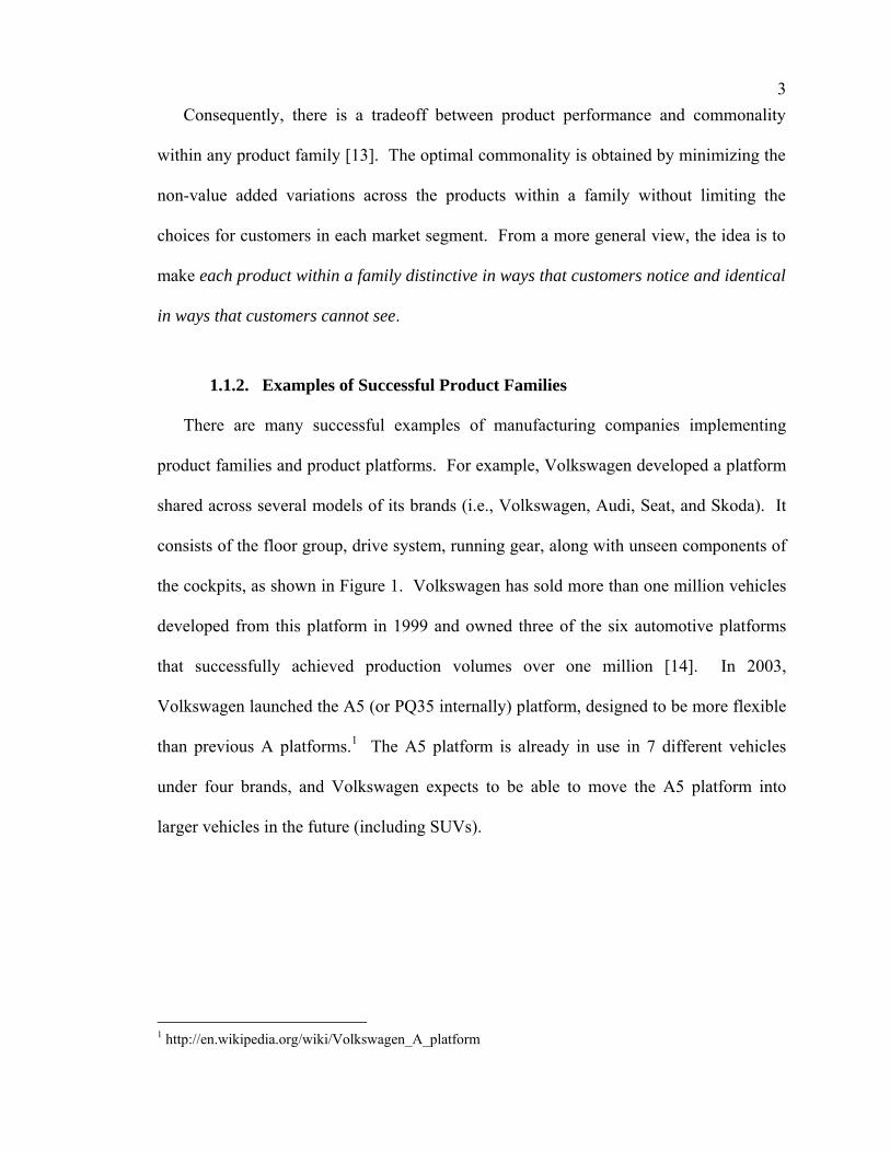
There are many successful examples of manufacturing companies implementing

product families and product platforms. For example, Volkswagen developed a platform

shared across several models of its brands (i.e., Volkswagen, Audi, Seat, and Skoda). It

consists of the floor group, drive system, running gear, along with unseen components of

the cockpits, as shown in Figure 1. Volkswagen has sold more than one million vehicles

developed from this platform in 1999 and owned three of the six automotive platforms

that successfully achieved production volumes over one million [14]. In 2003,

Volkswagen launched the A5 (or PQ35 internally) platform, designed to be more flexible

than previous A platforms.1 The A5 platform is already in use in 7 different vehicles

under four brands, and Volkswagen expects to be able to move the A5 platform into

larger vehicles in the future (including SUVs).

1 http://en.wikipedia.org/wiki/Volkswagen_A_platform

4

Figure 1 - Common components for Volkswagen platform [15]

Another example of a successful platform can be found in the Airbus A330/A340

family. It offers a choice of six models: two A330 versions plus four A340 versions. This

family covers capacities from 250 to 420 seats, as seen in Figure 2. All six aircraft share

common height, width and cockpit, but their fuselage lengths and the number of engines

(two or four) differ. The common cockpit has enabled the A330-200 to outsell the

Boeing 767-400ER [16].

5

Figure 2 - Configurations for the Airbus A330/A340 family2

1.1.3. Approaches to Product Family Design and Redesign

There are two recognized approaches to product family design [17]. The first is a

top-down (proactive platform) approach, wherein the company’s strategy is to develop a

family of products based on a product platform and its derivatives. There are many

examples of successful approaches such as Sony’s Walkmans [18] and Kodak’s one-

time-use cameras [19]. The second is a bottom-up (reactive redesign) approach, wherein

a company redesigns and/or consolidates a group of distinct products to standardize

components and thus reduce costs. For example, Black & Decker redesigned their

motors to reduce variety in their products [20]. Another successful example is Lutron

who redesigned its product line of lighting control around 15-20 standard components

that can be configured into more than 100 models specified by the customers [21].

Similar situations can be found when several companies merge, seeking to reduce

product proliferation by redesigning or consolidating one or more product lines.

2 http://www.airbus.com/product/a330_a340_commonality.asp

6Moreover, increased competition and globalization forces manufacturing companies to

benchmark their product lines against others versus benchmarking individual products,

particularly in the automotive industry [22]. John Deere [23] and Sunbeam [24] have

benefited from similar redesign efforts to reduce variety in their valve and food processor

lines respectively. Shirley [23] proposed a method to redesign a large product set to

improve product performances and to reduce manufacturing costs. The method consists

of two main steps: (1) core product selection and (2) cell selection. In the core product

selection, a set of core products (i.e., components that belong to a product platform) is

identified, based on similarities between the products and the time to (re)design the

variant products based on the core product. In cell selection, the products are allocated to

manufacturing cells to maximize throughput. While this method was proven to be

successful during manufacturing and redesign of product sets, the idea of product family

was not explicitly developed: the individual components (referred to products in Ref.

[23]) were grouped and redesigned to reduce manufacturing time, but the overall

commonality on the different instances of a product family was not considered. The

individual components were redesigned, rather than the products in a product family.

The effect of each component of the overall commonality was not considered. Moreover,

this method requires a lot of data that are not always readily available, and a lot of

estimates have to be proposed, such as the time to redesign a component based on

existing component. Meanwhile, the approach from Page [24], which is more customer-

centric, is to redesign an existing line of products using consumers’ evaluations of

possible new design with a marketing research technique (conjoint analysis). The first

step is to gather the consumers’ inputs that are used to redesign the products; several

7designs are then proposed, and the consumers choose their favorite ones. The next step is

to define market clusters to identify which design(s) fit(s) a specific market segment.

The clusters are then selected based on competition analysis (which products the

competition offer, for which segments) and based of projected profit analysis. While this

technique is very powerful to consider both consumers and competitions, it does not

address specifically how to redesign the products to increase commonality, but rather

chooses which product to manufacture. Moreover, the amount of data needed is

extensive, making this method very difficult, long and expensive to implement.

The few existing methods for product family redesign are very data-intensive or do

not focus on improving commonality; in this work, the focus is on supporting a bottom-

up approach to platform redesign, starting from an existing product family as discussed in

the next section.

1.2 Motivation for the Research

As more manufacturing companies seek to benchmark, redesign and consolidate their

product lines, there is an increased need for more systematic and consistent approaches to

product family redesign. While there are currently several studies regarding the measure

of product modularity and methods to achieve modularity during product redesign

[25,26], these studies focus on modularity within a single product. They do not focus on

product families or commonality directly. Moreover, there are currently no systematic

methods to analyze the degree of commonality in the design of a product family and

provide recommendations on how to improve it. Consequently, there is a need for less

information-intensive measures and methods that are useful during concept development

and layout design [13]. Developing such methods will provide product family designers

8with useful recommendations that could be implemented during product family redesign,

which will help reduce manufacturing costs.

1.3 Research Objectives

The main objective in this research is to develop a novel method for product family

redesign and demonstrate its use. While developing this method, three sub-objectives are

completed:

(1) Guidelines are proposed to reduce variation when collecting data during product

family dissection.

(2) Existing commonality metrics are reviewed and compared, and a new

commonality index is proposed.

(3) A genetic algorithm-based formulation to support component redesign within a

product family is introduced.

The proposed method uses data that are easy to collect or estimate as inputs: a list of

components in each product with related information (cost, material, manufacturing

process, etc.), as well as the redesign strategy (which components to keep unique, etc.).

The list of components is obtained from a Bill of Materials or if not available, the product

family is dissected using the guidelines provided to minimize variation when collecting

the data. A new commonality index then assesses the commonality in the entire family.

Using a genetic algorithm, the commonality index is then maximized, and

recommendations on how to improve the redesign of a product family are provided.

91.4 Outline of Dissertation

In the next chapter, a review of product family design strategies and analysis methods

is conducted. Chapter 3 introduces the proposed method, which is then detailed in

Chapter 4 (data collection for product family redesign), Chapter 5 (commonality indices

to assess the design of a product family), and Chapter 6 (optimization and redesign

recommendations). To demonstrate and validate this method, two example applications

are given in Chapter 7 (staplers from PaperPro, and valves from Flowserve), while

Chapter 8 gives closing remarks and future work.

10

CHAPTER 2 LITERATURE REVIEW

In this chapter, the following areas of research are investigated to lay the foundation

for the proposed method: product dissection and reverse engineering methods; product

family-based assessment methods, including modularity and commonality measurements;

and optimization algorithms (genetic algorithms in particular).

2.1. Product Dissection and Reverse Engineering

2.1.1. Product Dissection and Reverse Engineering Methods for Single

Products

This section reviews several methods that are commonly used in reverse engineering

of individual products. These include the Subtract and Operate Procedure [27], Force

Flow (Energy Field) Diagrams [27,28], and Design For Assembly [29]. The first

technique is a component elimination procedure, the second is a component combination

analysis, and the last one aims at minimizing unnecessary costs during manufacturing.

These methods help designers improve an existing design by eliminating redundant

components, simplifying component design and reducing assembly, etc. However, they

aim at improving the design of an individual product, rather than a family of products.

The Subtract and Operate Procedure (SOP) is a five-step procedure that aims at

eliminating redundant components in a product. The five steps are [27]:

(1) disassemble one component of the assembly,

(2) operate the system through its full range,

11(3) analyze the effect,

(4) deduce the sub-function of the missing component and,

(5) repeat the procedure for all the other components in the product.

SOP is a useful technique for understanding component functions during a reverse

engineering process. An example of SOP applied to a mechanism to oscillate an arm

through a designated angular range is shown in Figure 3 and Table 1. The arm is

connected to a rotary shaft that oscillates, but the range of rotation is constrained by two

pins and top-plate slots [28].

Figure 3 - SOP example device [28]

By looking at the effect of each part, the SOP highlights five parts that are redundant.

For example, the horizontal pin can be removed, as the arm will not slip against the shaft

because of the fixed vertical pins.

12Table 1 - Example SOP device worksheet [28]

Assembly/ Part No. Part description Effect of removal Deduced subfunction(s) &

affected customer needs

A-1 Shaft assembly 1 Top plate 360° rotary freedom Allow DOF regulate motion (arc) 2 Rotary shaft No torque transfer Transmit torque A-2 Arm assembly 1 Front rotary pin No effect Allow DOF support loads (durability) 2 Rear rotary pin No effect Allow DOF support loads (durability) 3 Rotary arm Transmit torque 4 Horizontal end pin No effect Support loads (safety) 5 Right vertical arm pin No effect Support loads 6 Left vertical arm pin No effect Support loads

Force Flow Diagrams are diagrams that represent the transfer of force through

product’s components [27,28]. The diagram created is used to identify the components

that have relative motion. This method aims at combining components, which leads to a

more integral architecture as opposed to a more modular architecture. Figure 4 shows an

example of application of the Force Flow Diagram for a stapler.

Figure 4 - Force flow diagram for a stapler [30]

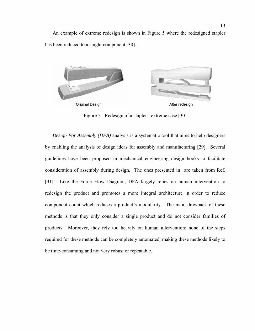
13An example of extreme redesign is shown in Figure 5 where the redesigned stapler

has been reduced to a single-component [30].

Original Design

After redesign

Figure 5 - Redesign of a stapler - extreme case [30]

Design For Assembly (DFA) analysis is a systematic tool that aims to help designers

by enabling the analysis of design ideas for assembly and manufacturing [29]. Several

guidelines have been proposed in mechanical engineering design books to facilitate

consideration of assembly during design. The ones presented in are taken from Ref.

[31]. Like the Force Flow Diagram, DFA largely relies on human intervention to

redesign the product and promotes a more integral architecture in order to reduce

component count which reduces a product’s modularity. The main drawback of these

methods is that they only consider a single product and do not consider families of

products. Moreover, they rely too heavily on human intervention: none of the steps

required for these methods can be completely automated, making these methods likely to

be time-consuming and not very robust or repeatable.

14

Figure 6 - Set of guidelines for DFA [31]

2.1.2. Product Family-based Analysis Methods

This section presents an overview of existing research on the evaluation of product

modularity and commonality and methods to achieve modularity and commonality in

product family redesign. These measures and methods vary considerably in purpose and

process: the nature of the data gathered (some are extensively quantitative while some are

more qualitative), the ease of use, and the focus of the analysis. However, they all share

the goal of helping designers resolve the tradeoff between too much commonality (i.e.,

lack of distinctiveness of the products) and not enough commonality (i.e., higher

production costs).

15

Modularity in Product Family Design

Modularity arises from the decomposition of a product into subassemblies and

components [26]. Ulrich [32] defines the product architecture as “(1) the arrangement of

functional elements; (2) the mapping from functional elements to physical components;

(3) the specification of the interfaces among interacting physical components”. This

division facilitates the standardization of components and increases product variety

[33,34]. Most of the methods to measure modularity in a product family are based on the

use of modularity matrices to show the relationships between the components in a family.

Some examples are the matrices from Sosale, et al. [22] that are filled with physical,

spatial and geometric interactions; the design structure matrix from Pimmler and

Eppinger [35]; and the interaction and suitability matrices developed by Huang and

Kusiak [36,37]. These matrices fit the need for component manipulation and

comparison. The evaluation of the degree of modularity of a product family enables

designers to find appropriate modules to improve a product’s design. A recent overview

of modularity and its benefits can be found in Ref. [25], and a comparison of existing

measures of product modularity is documented in Ref. [26]. What is important to note is

that all of these measurements are information-intensive and are therefore quite

cumbersome to compute. That is why few, if any, complex examples have been used in

the research on modular product design.

The modularity matrices and modularity measurements described previously can be

used to cluster components into modules for each product. Most of them are based on the

following steps:

16(1) measurement of the modularity,

(2) manipulation of the information using modularity matrices, and

(3) measurement of the new modularity and iteration.

A review of these modularity methods is given in Ref. [26]. One problem with all of

these methods is that they require a considerable amount of information that is not always

readily available. Moreover, these methods are applied to single products only, and

although they can be potentially used across products in a product family, no method

using modularity at the product family level can be found in the literature.

Commonality Indices

To measure the commonality within a family of products, several commonality

indices have been proposed. A commonality index is a metric to assess the degree of

commonality within a product family. It is based on different parameters such as the

number of common components, component costs, manufacturing processes, etc. These

indices are often the starting point when designing a new family of products or when

analyzing an existing family. They are intended to provide valuable information about

the degree of commonality achieved within a family and how to improve a product’s

design to increase commonality in the family and reduce costs; however, there have been

only limited comparisons between many of these commonality indices and their

usefulness for product family redesign [38,39]. Several component-based indices are

summarized in Table 2, followed by a short description of each index.

17Table 2 - Commonality indices for comparative study

Name Developed by Commonality measure for

No Commonality

Complete Commonality

DCI Degree of Commonality Index

Collier [6] The whole family 1 ∑+

+=

Φ=di

ijj

1

β

TCCI Total Constant Commonality Index

Wacker and Trelevan [40] The whole family 0 1

PCI Product Line Commonality Index

Kota, et al. [41] The whole family 0 100

%C Percent Commonality Index

Siddique, et. al [1] Individual products within a family 0 100

CI Commonality Index

Martin and Ishii [42,43] The whole family 0 1

CI(C) Component Part Commonality Jiao and Tseng [44] The whole family 1 ∑∑

= =

Φ=d

j

m

iij

1 1α

Degree of Commonality Index

The Degree of Commonality Index (DCI) is the most traditional measure of

component part standardization [6]. It reflects the average number of common parent

items per average distinct component:

dDCI

di

ijj∑

+

+=

Φ= 1

(1)

where:

Φj = number of immediate parents component j has over a set of end items or product structure level(s).

d = total number of distinct components in the set of end items or product structure level(s).

i = the total number of end items or the total number of highest level parent items for the product structure level(s).

Component item = any inventory item (including a raw material) other than an end item that goes into higher level items.

End item = finished product or major subassembly subject to a customer order or sales forecast.

Parent item = any inventory item that has component parts.

18

The DCI has no fixed boundaries, ranging between 1 and β, where β is defined in Table 2.

The main advantage of the DCI is its ease of computation. Its primary limitation is that it

is a cardinal measure without fixed boundaries; hence, it is difficult to estimate the

increase in commonality while redesigning a family and to compare different families of

products.

Total Constant Commonality Index

The Total Constant Commonality Index (TCCI) is a modified version of the DCI

[40]. Contrary to the DCI, which is a cardinal index (and hence an absolute increase in

commonality is not possible to measure), it is a relative index that has absolute

boundaries ranging from 0 to 1:

1

11

1−Φ

−−=

∑=

d

jj

dTCCI (2)

The absolute boundaries of TCCI facilitate comparisons between product families

and within a family of products during redesign.

The Product Line Commonality Index

Contrary to the indices that simply measure the percentage of components that are

common across a product family (and hence penalizing families with a broader feature

mix), the Product Line Commonality Index (PCI) measures and penalizes the differences

in the non-unique components, given the product mix [41]. The PCI has fixed boundaries

that range from 0 to 100. The PCI is given by:

19

100*

1 1

1 1

∑ ∑

∑ ∑

= =

= =

−

−= P

i

P

iii

P

i

P

iii

MinCCIMaxCCI

MinCCICCIPCI (3)

where:

CCi = Component Commonality Index for component i. = ni * f1i * f2i * f3i MaxCCIi = Maximum possible Component Commonality Index for component i. = N MinCCIi = Minimum possible Component Commonality Index for component i. = ni * 1/ni * 1/ni * 1/ni = 1/ni

2 P = Total number of non differentiating components that can potentially be

standardized across models. N = Number of products in the product family. ni = Number of products in the product family that have component i. f1i = Size and shape factor for component i. = Ratio of the greatest number of models that share component i with identical

size and shape to the greatest possible number of models that could have shared component i with identical size and shape (ni).

f2i = Materials and manufacturing processes factor for component i. = Ratio of the greatest number of models that share component i with identical

materials and manufacturing processes to the greatest possible number of models that could have shared component i with identical materials and manufacturing processes (ni).

f3i = Assembly and fastening schemes factor for component i. = Ratio of the greatest number of models that share component i with identical

assembly and fastening schemes to the greatest possible number of models that could have shared component i with identical assembly and fastening schemes (ni).

When PCI = 0, either none of the non-unique components are shared across models,

or if they are shared, their sizes/shapes, materials/manufacturing processes, and assembly

processes are all different. When PCI = 100, it indicates that all the non-unique

components are shared across models and that they are of identical size and shape, made

using the same material and manufacturing process, and the assembly and fastening

methods are identical. This index focuses on commonality that should exist between

products that share common or variant components rather than on the unique components

20that differentiate the products. It provides a single measure for the entire product family,

but it does not offer insight into the commonality of the individual products.

Percent Commonality Index

The Percent Commonality Index (%C) is based on three main viewpoints: (1)

component viewpoint, (2) component-component connections viewpoint, and (3)

assembly viewpoint. Each of these viewpoints results in a percentage of commonality,

which can then be combined to determine an overall measurement of commonality for a

platform by using appropriate weights for each item [1]. The component viewpoint

measures the percentage of components of a platform that are common to different

models and is the percent commonality of components Cc:

componentsuniquecomponentscommoncomponentscommonCc +

=*100

(4)

The component-component connections viewpoint measures the percentage of

common connections between components, Cn:

sconnectionuniquesconnectioncommonsconnectioncommonCn +

=*100

(5)

Similarly, the assembly viewpoint measures the percentage of common assembly

sequences. Two indices are used: (1) Cl, to measure the percentage of common assembly

sequences, and (2) Ca, to measure the percentage of common assembly workstations:

loadingcomponentassemblyuniqueloadingcomponentassemblycommonloadingcomponentassemblycommonCl +

=*100

(6)

nworkstatioassemblyuniquenworkstatioassemblycommonnworkstatioassemblycommonCa +

=*100

(7)

21These four values can then be combined into an overall platform commonality

measure; the weighted-sum formulation is the most popular [1]:

(8)

where: Ii = importance (weighting factors) where ΣIi = 1. Ci = % commonality as previously described.

The resulting %C ranges from 0 to 100. This index takes the manufacturing process

into consideration; moreover, it can be adapted to different strategies using weighting

factors. The disadvantage is that the measure is applied to each platform and not the

family as a whole, which increases the computational expense of this measure.

Commonality Index

Proposed by Martin and Ishii [42,43], the Commonality Index (CI) is a measure of

unique components that is similar to the DCI proposed by Collier. CI ranges from 0 to 1:

(9))

where: u = number of unique components. pj = number of components in model j. vn = final number of varieties offered.

A higher CI is better since it indicates that the different varieties within the product

family are being achieved with fewer unique components. The CI can be interpreted as

the ratio between the number of unique components in a product family and the total

number of components in the family.

22Component Part Commonality Index

Proposed by Jiao and Tseng [44], the Component Part Commonality Index (CI(C)) is

an extended version of the DCI that takes into account product volume, quantity per

operation, and the cost of each component:

(10))

where: d = total number of distinct component parts used in all the product structures of a

product family. j = index of each distinct component part. Pj = price of each type of purchased components or the estimated cost of each

internally made component part. m = total number of end products in a product family. i = index of each member product of a product family. Vi = volume of end product i in the family. Φij= number of immediate parents for each distinct component part dj over all the

products levels of product i of the family.

= total number of applications (repetitions) of a distinct component part dj

across all the member products in the family. Qij = quantity of distinct component part dj required by the product i.

The CI(C) has ‘moving’ boundaries that range from 1 to α. The CI(C) gives very useful

information, as it takes the cost of each component into consideration. For instance, a

very expensive component common throughout a family has more influence than a

component that is very cheap and different from one product to another. A disadvantage

in CI(C) is in estimating the quantity and cost information needed to compute the index. It

is also noteworthy that this index can be subject to errors in some specific cases; a

corrected version of the formula is proposed in Ref. [45].

23

Other Commonality indices

Other commonality indices can be found in the literature, but they are much more

information intensive and hence difficult to apply. Martin and Ishii [46] proposed a

Generational Variety Index to help identify which components are likely to change over

time in order to meet future market requirements and a Coupling Index to measure the

coupling between these components. A Functional Similarity Index was introduced by

McAdams and his co-authors [47,48] to assist in concept development and modular

product design. Finally, indices for measuring the Degree of Variation within a scale-

based product family have also been proposed [13,49,50].

Optimization-Based Approaches for Product Family Redesign

Several optimization approaches have been developed to help determine the best

design parameters for a product family; A summary of the existing optimization-based

approaches for product family redesign can be found in Ref. [51]. A problem with most

of the methods is that they require the specification of the platform a priori to the

optimization. This is not ideal, as a design team would prefer to use optimization to

explore varying levels of platform commonality to help identify which variables to make

common and unique within the family [52]. Various algorithms for product family

redesign are employed, from exhaustive search techniques (when the design space is

small), to linear and nonlinear programming and derivative-free methods such as genetic

algorithms, simulated annealing, pattern search. However, due to the complexity and

combinatorial nature of product family redesign problems, many researchers recommend

24and use genetic algorithm [52-56]. In this research, a genetic algorithm is employed;

more details are given in the next section.

2.2. Genetic Algorithms

Evolution-based algorithms such as genetic algorithms (GAs) [57,58] are flexible,

efficient and robust search algorithms [59]. Because of these properties, the use of

evolutionary search to optimize existing designs is widespread. GAs are adaptive

stochastic optimization algorithms involving search and optimization. Instead of working

with a single solution at each iteration, a GA works with a number of solutions

(collectively known as a population). GAs are based on the notion of “survival of the

fittest”, and they operate by searching for and choosing optimal solutions in much the

same way that natural selection occurs. GAs only use the objective function while

searching for optimized result and not the derivatives; therefore, it is a direct search

method. GAs work with a coding of the parameter set (set of strings/individual

chromosomes), not the parameters themselves and use probabilistic transition rules [59].

GA methods optimizing product family design utilize the stochastic search nature of

genetic algorithms to find combinatorial designs within the search space. GAs appear

well suited for solving combinatorial problems typical in product family [52,56].

Usually there are only two main components of most GAs that are problem-

dependent: (1) the problem encoding and (2) the evaluation function. When the GA is

implemented, it is usually done in a manner that involves the following cycle:

- Evaluate the fitness of all of the individuals in the population.

25- Create a new population by reproduction. The reproduction process for a pair of

chromosomes involves duplicating the two individual chromosomes (the “parents”)

and then choosing a place (site) on the chromosomes to crossover (or switch)

information between them. This results in two new “children” chromosomes in the

population, which could have higher fitness values than their “parents”. Mutation

can also occur when decision variable values in a chromosome are randomly

changed.

- The old population is then discarded, and a new iteration is started using the new

population.

Every iteration of the GA is referred to as a generation. The exchange of information

between chromosomes during crossover allows the algorithm to converge to a global,

rather than a local, optimum [59]. Even though the operators are simple, GAs are highly

nonlinear, massively multifaceted, stochastic, and complex.

While many optimization have been employed for product family design, many

researchers advocate the use of GAs for product family design; this research proposes the

use a genetic algorithm to optimize the design of an existing product family. More

details on the GA used in this work can be found in Chapter 6.

2.3. Remarks on Group Technology

Extensive literature can be found on the topic of Group Technology (GT). GT “is a

disciplined approach to identify things such as parts, processes, equipment, tools, people

or customer needs by their attributes, analyzing those attributes looking for similarities

between and among the things; grouping the things into families according to similarities;

26and finally increasing the efficiency and effectiveness of managing the things by taking

advantage of the similarities” [60]. GT is typically employed for two primary

applications in manufacturing companies. The most publicized of these applications if

the process of restructuring the shop floor to a cellular layout by identifying part families

and machine cells [61,62]. The second application of GT is the classification and coding

of parts. The most common usage of classification and coding systems is for the retrieval

of designs (from a design database) to be used as the basis for new designs and for

determining part families and cells [63]. The goal in this research is not to group

components or manufacturing processes based on their similarity, but rather redesign

components to increase commonality; hence, the proposed research does not focus on

using GT.

2.4. Summary

This chapter reviewed existing tools for product and product family redesign. While

methods have been developed to assess the commonality in a product family and to

redesign individual products, there are no systematic methods to support product family

redesign. In the next chapter, a method to support product family redesign is introduced

that reuses some of the tools introduced in this chapter to (1) assess the design of an

existing product family and (2) help redesign the product family.

27

CHAPTER 3 METHOD FOR PRODUCT FAMILY REDESIGN

The objective in this research is to develop and implement a systematic and consistent

method for product family redesign. In this chapter, the proposed method is introduced,

and its phases are explained.

3.1 Introduction

As discussed in Chapters 1 and 2, very few methods for product family redesign can

be found in the literature, and most of them are hard to implement and repeat. This work

proposes and implements a systematic and consistent method based on the use of a

commonality index to improve platform commonality during product family redesign by

giving specific recommendations for each component based on simple BOM data:

- Systematic and consistent computation: unlike most of the research, in which the

improvement of the commonality in a family is the result of many human computations,

hence applied to very small case studies, the method proposed minimizes human

intervention to only the input data phase, improving accuracy, repeatability and the

robustness of the results.

- Use of a commonality index: commonality indices are useful metrics to assess the

design of a product family (as discussed in Section 2.1.2).

- Specific recommendations for each component: most of the existing methods to

improve the design of a product family are based on grouping the components into

modules e.g., [26]; in the proposed method, the effect of each component on the level of

28commonality of the product family is also studied, and recommendations are made on

how to redesign specific parameters of the components.

- Use of simple BOM data: unlike most of the existing methods that require a

considerable amount of information that is not always readily available, the proposed

method is based on data that are relatively easy to acquire through dissection or a Bill of

Materials.

These aspects are achieved through the method shown in Figure 7. The first phase is

data collection. Information for each component in each product in the family is

collected, either directly using an existing Bill of Materials or by dissection (see Section

3.2 and Chapter 4). The second phase is commonality assessment of the family using

appropriate metrics (see Section 3.3 and Chapter 5). The third and fourth phases are the

generation of recommendations using optimization tools (see Section 3.4 and Chapter 6).

Each phase is described next.

29

Figure 7 - Proposed method for product family redesign

3.2 Phase 1: Data Collection

The first phase in this method is to obtain the necessary data for the product family

being analyzed. If the information is already available through a Bill of Materials, for

example, the user simply enters the appropriate data. If the information is not readily

available, a dissection of the products in the family is required. To ensure consistency

during dissection, each product within the family is dissected to the lowest level possible,

i.e., the components cannot be further divided into subassemblies. However, some

assemblies can be difficult, if not impossible, to dissect to that extent, such as electronic

printed circuit boards, which can be taken as a single component for analysis. To

minimize variation when data are collected, a list of possible choices for material,

manufacturing process and assembly scheme is given to the designer (see Appendix A.1

30for materials, Appendix A.2 for manufacturing processes, and Appendix A.3 for

assembly and fastening schemes) based on Ref. [64]. This list is not exhaustive, and the

designer can add additional data as needed. For the production volume and the unit cost,

the data can be either very easy to obtain directly from a company, but if not available,

costs should be estimated using appropriate methods (such those found in Ref. [65]). The

data collected during product dissection can vary greatly, depending on who is doing the

dissection. Chapter 4 describes guidelines developed as part of this research to minimize

variation during product family dissection.

3.3 Phase 2: Commonality Assessment

To measure the commonality within a product family, several commonality indices

have been proposed in the literature (see Section 2.2). The indices employed in this

research are component-based, and they can be easily computed with relatively limited

information, such as the components in the products, their materials, etc. The indices can

be computed using the data collected in Phase 1. The information that can be obtained

using these commonality indices is discussed in Chapter 5, and a new commonality index

is also proposed to address the limitations of the existing commonality indices.

3.4 Phase 3: Optimization and Phase 4: Redesign

In this research, a Genetic Algorithm (GA) is employed to redesign a product family.

The GA uses the new commonality index proposed in Chapter 5 to assess the design of

an existing product family and to maximize its commonality. Once the optimization is

complete, a redesign sequence is recommended that can be compared to the original

31design. Two main types of information are given using the GAs: (1) at the product

family level, if there exists more than one design for a particular family, then the

algorithm assesses each redesign suggestion and classifies them according to the initial

commonality and the ease of redesign; (2) at the component level, a list of components to

redesign is proposed to achieve the highest commonality with a minimum number of

changes. More details are given in Chapter 6.

3.5 Conclusions

The proposed method introduced in this chapter uniquely addresses the issue of

product family redesign using a commonality index to assess and help redesign a product

family at the component level. The next three chapters (Chapters 4, 5 and 6) detail this

method shown in Figure 7, which is fully implemented and validated in Chapter 7

through two example applications.

32

CHAPTER 4 USING DISSECTION TO COLLECT PRODUCT DATA:

GUIDELINES TO MINIMIZE VARIATION

In this chapter, a set of guidelines for dissecting a product family is developed,

aiming at minimizing variation due to involuntary input variation (“noise”) when

computing commonality indices in order to yield more accurate and repeatable results.

The guidelines are created by conducting two human experiments to study actual

dissection methods. The proposed guidelines are validated through these experiments.

4.1 Introduction

When product design information is not readily available, dissection needs to be

performed on the product family being redesigned to collect information to compute

commonality indices for product family redesign. The information needs to be consistent

so that the commonality assessment based on this data is robust. The problem with

product dissection is that it is a heavily human-based activity, and variation in the

information collected can occur, such as different levels of dissection, components

forgotten or skipped, and different interpretation of what is meant to be “common”. In

order to minimize this variation, guidelines are developed in this chapter and validated

using two human-based experiments, where different sets of people were asked to: (1)

dissect various product families, (2) collect data from the dissection, and (3) compute a

commonality index, namely, the Product Line Commonality Index (PCI [41]). In the first

experiment, no guidelines are given to the teams, and the sources of variation are

identified. Guidelines are then proposed to minimize this variation, and a second

33experiment is conducted, with the proposed guidelines given to the teams. In Section 4.2,

the first experiment is described, and Section 4.3 describes the second experiment.

Section 4.4 compares the results obtained in both experiments, and Section 4.5 gives

summary remarks.

4.2 Experimental Method and Results from the First Experiment

In this section, the experimental method as well as the results from the first

experiment are described. The first product dissection activity consisted of five teams

dissecting and analyzing three different families of products, each containing four

products. Based on their results, three main sources of the variation that occurred during

the dissection of the products and calculation of the PCI were identified: (1) different

levels of dissection, (2) components omitted from the analysis, and (3) different values

for the factors used to compute the PCI. Recommendations for reducing the variation are

then developed based on these findings.

4.2.1. Experimental Method

The experiment was conducted in the Design Studio and Product Dissection

Laboratory (314 Hammond Building) within the Center for Engineering Design and

Entrepreneurship3. The laboratory has basic tools for dissection (e.g., screwdrivers,

wrenches, pliers, etc.) while providing ample room for laying out the components for

analysis; the room also has several computers that were made available to each group to

complete an Excel spreadsheet to compute the PCI (see Chapter 2 for its formulation).

Figure 8 shows a picture of the students working in the lab during the experiment.

3 http://www.cede.psu.edu/

34

Figure 8 - Product dissection studio

While some commonality indices are based only on information from the Bill of

Materials, other indices, such as the PCI, are more subjective in nature with results

varying from user to user. For example, when computing the PCI, the values of f1i, f2i

and f3i for each component can vary depending upon the user’s knowledge and point of

view: what exactly is ‘same size’ or ‘same shape’?, what if two are components are

identical except in color?, etc. At the time of the experiment, the PCI was the index that

was the most data intensive; hence the PCI was chosen for the experiment. The

guidelines that are obtained after this experiment can also be applied to less information-

intensive commonality indices to minimize their variation.

In order to quantify the variation in the PCI, the product dissection activity was set up

such that the results from each group’s analysis could be pooled to examine the variation

within the estimates of platform commonality using the PCI. This was accomplished

using five teams of four to five people, and three families of products consisting of four

products each: Kodak and Fujifilm one-time-use cameras and Mr. Coffee coffeemakers

(see Table 3). These families were chosen so that comparisons could be made both

within a family and across similar families (i.e., the one-time-use cameras). The products

35are also readily available in the market and relatively inexpensive: the cameras cost $5-

$12 each while the coffeemakers cost $20-$50 each.

Table 3 - Products dissected and analyzed Family Product 1 Product 2 Product 3 Product 4

Kodak (2 sets)

MAX Outdoor

MAX Flash

Funsaver 35

MAX Water & Sport

Fujifilm

Quicksnap Outdoor

Quicksnap flash – old

Quicksnap flash - new

Quicksnap waterproof

Mr. Coffee (2 sets)

TFX20

TFX23

TF13

ESX33

Each team was instructed to perform the following tasks.

1. Read an overview of the experiment and sign informed consent form.

2. Dissect each product in the family to the lowest level possible, i.e., to the point when the components cannot be divided into further subassemblies.

3. Identify the different components as being either: common to each product within the family, variant of one another in each product within the product family, or unique to each product within the product family.

4. Take a picture of each product after it is dissected using the digital camera provided in the laboratory. This picture should show all the components for each product and should include captions that should be used when completing the Excel spreadsheet.

5. Complete the Excel spreadsheet template where the rows represent the components sorted by name, and the columns represent the different products in the family. An additional column was used to identify the commonality among components in each product.

6. Compute the PCI for one of the other product families that was dissected by another team using a new Excel spreadsheet template.

36The instructions were deliberately kept “vague” so that the variation due to different

understanding of the definitions between the different teams could be analyzed.

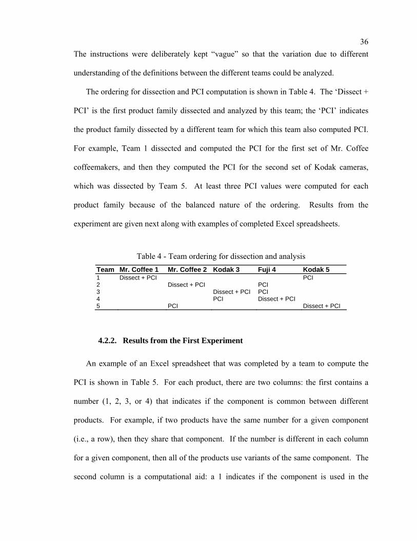
The ordering for dissection and PCI computation is shown in Table 4. The ‘Dissect +

PCI’ is the first product family dissected and analyzed by this team; the ‘PCI’ indicates

the product family dissected by a different team for which this team also computed PCI.

For example, Team 1 dissected and computed the PCI for the first set of Mr. Coffee

coffeemakers, and then they computed the PCI for the second set of Kodak cameras,

which was dissected by Team 5. At least three PCI values were computed for each

product family because of the balanced nature of the ordering. Results from the

experiment are given next along with examples of completed Excel spreadsheets.

Table 4 - Team ordering for dissection and analysis Team Mr. Coffee 1 Mr. Coffee 2 Kodak 3 Fuji 4 Kodak 5 1 Dissect + PCI PCI 2 Dissect + PCI PCI 3 Dissect + PCI PCI 4 PCI Dissect + PCI 5 PCI Dissect + PCI

4.2.2. Results from the First Experiment

An example of an Excel spreadsheet that was completed by a team to compute the

PCI is shown in Table 5. For each product, there are two columns: the first contains a

number (1, 2, 3, or 4) that indicates if the component is common between different

products. For example, if two products have the same number for a given component

(i.e., a row), then they share that component. If the number is different in each column

for a given component, then all of the products use variants of the same component. The

second column is a computational aid: a 1 indicates if the component is used in the

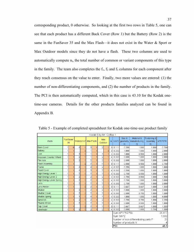
37corresponding product, 0 otherwise. So looking at the first two rows in Table 5, one can

see that each product has a different Back Cover (Row 1) but the Battery (Row 2) is the

same in the FunSaver 35 and the Max Flash—it does not exist in the Water & Sport or

Max Outdoor models since they do not have a flash. These two columns are used to

automatically compute ni, the total number of common or variant components of this type

in the family. The team also completes the f1, f2 and f3 columns for each component after

they reach consensus on the value to enter. Finally, two more values are entered: (1) the

number of non-differentiating components, and (2) the number of products in the family.

The PCI is then automatically computed, which in this case is 43.10 for the Kodak one-

time-use cameras. Details for the other products families analyzed can be found in

Appendix B.

Table 5 - Example of completed spreadsheet for Kodak one-time-use product family

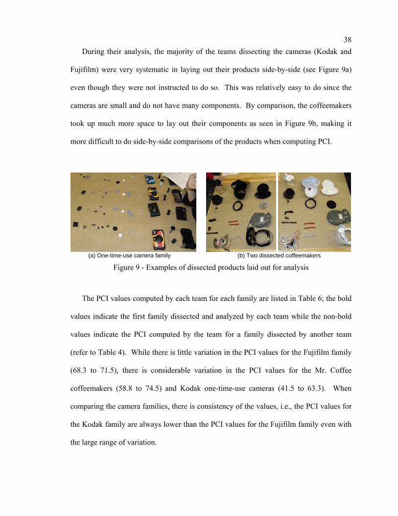
38During their analysis, the majority of the teams dissecting the cameras (Kodak and

Fujifilm) were very systematic in laying out their products side-by-side (see Figure 9a)

even though they were not instructed to do so. This was relatively easy to do since the

cameras are small and do not have many components. By comparison, the coffeemakers

took up much more space to lay out their components as seen in Figure 9b, making it

more difficult to do side-by-side comparisons of the products when computing PCI.

(a) One-time-use camera family (b) Two dissected coffeemakers

Figure 9 - Examples of dissected products laid out for analysis

The PCI values computed by each team for each family are listed in Table 6; the bold

values indicate the first family dissected and analyzed by each team while the non-bold

values indicate the PCI computed by the team for a family dissected by another team

(refer to Table 4). While there is little variation in the PCI values for the Fujifilm family

(68.3 to 71.5), there is considerable variation in the PCI values for the Mr. Coffee

coffeemakers (58.8 to 74.5) and Kodak one-time-use cameras (41.5 to 63.3). When

comparing the camera families, there is consistency of the values, i.e., the PCI values for

the Kodak family are always lower than the PCI values for the Fujifilm family even with

the large range of variation.

39Table 6 - Initial PCI values

Team Mr. Coffee 1 Mr. Coffee 2 Kodak 3 Fuji 4 Kodak 5 1 63.2 43.1 2 58.8 71.5 3 55.3 70.9 4 63.3 68.3 5 74.5 41.5

After the experiment, the results were analyzed in more detail to identify the sources

of these differences. The dissection portion of the experiment is first analyzed, followed

by the computation portion of the experiment. Three major contributors to the variation

in PCI was identified, as shown in Figure 10:

1. Different levels of dissection 2. Components omitted from analysis 3. Different values for fji factors

Discussion about the impact and extent of each of these contributors follows.

Figure 10 - Three different sources of variation identified during the first experiment

Different levels of dissection: Some teams dissected their products more thoroughly,

which lead to more components being identified and included in the PCI calculation. For

example, the flash in the one-time-use cameras was considered as one component by

several teams, while others dissected it more thoroughly to identify two distinct

components, namely, the flash cover and the flash printed circuit board (see Figure 11).

Similar variations existed among the coffeemakers, many of which included printed

circuit boards and lots of wiring; some teams dissected these to a greater level of detail

40than others. Finally, there were also some differences in naming components for

analysis, but this was not a major contributor to the differences in the PCI since it did not

change the number of components being analyzed.

Flash Cover

Flash Printed Circuit Board

Figure 11 - Example of analyzed components for the Kodak one-time-use cameras

Components omitted from analysis: A much larger contributor to the variation was

components being omitted from analysis, either voluntarily or involuntarily. First, some

teams forgot to include components in their analysis; for example, the camera film,

although obviously a major component, was (involuntarily) skipped in the analysis by

one team (see Table 7). Second, teams were instructed not to consider components such

as screws, electrical wires, etc. since they can be easily standardized; however, some

teams included these components in their analysis while others omitted them. Finally,

some components were omitted from the analysis if the team did not dissect a

subassembly to a sufficient level of detail as mentioned previously.

In order to determine the effect of the variation introduced during dissection, the

results from Table 6 were “corrected” to take into consideration the different levels of

dissection and omitted components. First, each component within each family was

renamed using a common name. Second, the unique components were removed along

with screws, fasteners, etc. While the unique components should not be considered when

calculating the PCI, it is also recommended not to include components that can be easily

41standardized in the analysis as it artificially inflates the value of PCI. Finally, any

omitted components from a team’s analysis were added using the arithmetic average of

the fji factors attributed by the other teams; a similar approach is used during the analysis

of experimental designs when data are missing [66]. The rightmost column in Table 7

indicates the omitted components from each team’s analysis for the four Kodak one-time-

use cameras.

Table 7 - Summary of omitted components for each Kodak camera

Using the “completed” data, each team’s PCI value was recalculated, and the

“corrected” PCI values are summarized in Table 8. This “corrected” PCI removed the

variation due to missing components in the analysis. The percent change in the PCI value

is noted to the right of the “corrected” PCI value in parentheses. Despite these

corrections, the trends remained the same. The PCI variation is still considerable for the

Mr. Coffee coffeemakers and Kodak one-time-use cameras (54.4 to 79.0 and 47.0 to

64.0, respectively), while the variation remains small in the Fujifilm one-time-use

42cameras (68.3 to 71.5). Using the “corrected” data, difference in values of fji factors

could now be analyzed.

Table 8 - “Corrected” PCI values Team Mr. Coffee 1 Mr. Coffee 2 Kodak 3 Fuji 4 Kodak 5 1 63.8 (+1.0%) 48.9 (+13.5%) 2 54.4 (-7.5%) 68.6 (-4.1%) 3 54.8 (-0.1%) 72.4 (+2.1%) 4 64.0 (+1.1%) 65.2 (-4.5%) 5 79.0 (+6.0%) 47.0 (+ 13.3%)

Differences in values for fji factors: For a given component, different teams attributed

different values to the fji factors, which is the major source of variation that was found

when computing PCI. Consider the summary of the analysis of each team for the Kodak

one-time-use cameras shown in Table 9. A ‘1’ in any of the last three columns indicates

that the value of that fji factor differs at least once among the four teams’ analyses. As

seen in the figure, factor f1i has a different value for 17 out of the 24 rows (components);

f2i varies 9 out of 24 rows, and f3i varies 7 out of 24 rows. Details for the other product

families analyzed can be found in Appendix C. Using these numbers, the ratio of the

“number of components where the factor fji is different” to the “total number of

components” is computed, e.g., for f1i the ratio is 1-(24-17)/24 = 70.8%. Table 10

summarizes these ratios for all three families. Based on these ratios, one can note that

there is much less variation in values assigned to the f3i factor than for either f1i or f2i. For

the “assembly and fastening scheme” factor, f3i, the teams were able to more consistently

identify the commonality of connections and the assembly of the components with less

variation. They were able to clearly compare the assembly method between two

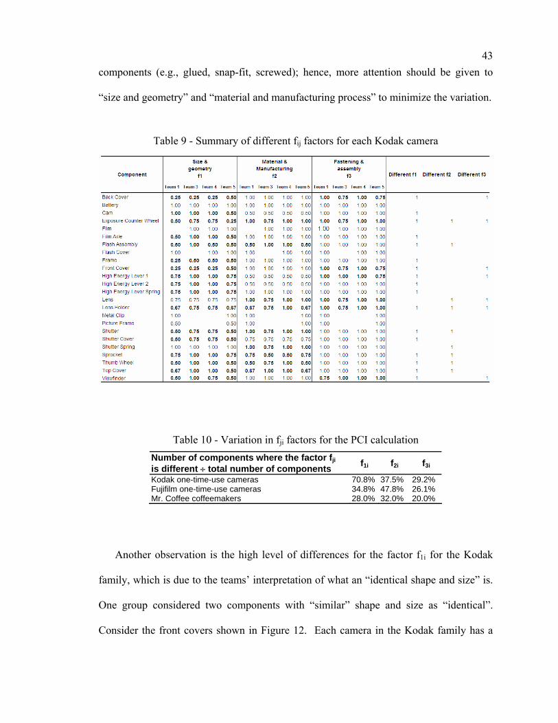
43components (e.g., glued, snap-fit, screwed); hence, more attention should be given to

“size and geometry” and “material and manufacturing process” to minimize the variation.

Table 9 - Summary of different fij factors for each Kodak camera

Table 10 - Variation in fji factors for the PCI calculation Number of components where the factor fji is different ÷ total number of components f1i f2i f3i

Kodak one-time-use cameras 70.8% 37.5% 29.2% Fujifilm one-time-use cameras 34.8% 47.8% 26.1% Mr. Coffee coffeemakers 28.0% 32.0% 20.0%

Another observation is the high level of differences for the factor f1i for the Kodak

family, which is due to the teams’ interpretation of what an “identical shape and size” is.

One group considered two components with “similar” shape and size as “identical”.

Consider the front covers shown in Figure 12. Each camera in the Kodak family has a

44front cover, and all the covers have a different shape. The corresponding f1i is 1/4;

however, one team considered that two of the covers were “identical” because they were

very similar in size and shape, and they assigned f1 a value of 1/2.

Figure 12 - Front covers for the Kodak one-time-use cameras

For the f2i factor, the differences are due to a misinterpretation of what an “identical

material” is. Some teams considered that two components made of the same material

(such as plastic) but with different colors (such as black for one and blue for the other)

are still “identical material”, while other teams considered these components different.

Such a component is illustrated in Figure 13.

Kodak Max Flash (black)

Kodak Max Outdoor (blue)

Figure 13 - Example of a “similar” component in the Kodak one-time-use cameras

In summary, the differences between the fji values arose primarily from a lack of

precise and accurate definitions of terms. The term “identical” was interpreted

differently by each group, resulting in large variation in the PCI values due to the values

assigned to the fji factors.

454.2.3. Recommendations to Minimize Variation

Three main sources of variation that occur during the dissection of the products and

calculation of the PCI were identified in this first experiment: (1) different levels of

dissection, (2) components omitted from the analysis, and (3) different values for the

factors used to compute the PCI. Examples of each were discussed using the results from

the four Kodak one-time-use cameras. The results for the other families can be found in

the appendices.

There are several implications based on these findings. First, variation that occurs

during dissection can be reduced by making sure that each team dissects their products to

the same level, and specific rules should be used to define this. For example, a

component could be considered one element if it is made of one material. For the

components that are hard to dissect, rules for leaving them as subassemblies should be

given, e.g., electronic printed circuit boards are always considered as one element.

Finally, a detailed component list would be helpful to ensure that components are named

properly and minimize the omission of components from the analysis. While this may

seem counter-intuitive (i.e., why proceed to a dissection if the list of parts is already

available?), in fact, while it is relatively easy to find a component list for each product,

the associated information required to compute the commonality indices may not be as

readily available.

During the calculation of PCI, detailed definitions should be included for the

different factors, and these rules should be systematically applied by each team. For

example, a list of possible manufacturing processes, materials, and assembly and

fastening schemes must be established for the f2 and f3 factors. Teams could then pick

46from this list when deciding how components were assembled and fastened together. By

creating specific rules, the variation of the PCI can be greatly reduced to provide a more

repeatable and consistent measure of platform commonality for use during product family

design. The second experiment described next takes into account these recommendations,

and the variation in the results are shown to be significantly reduced.

4.3 Experimental Method and Results for the Second Experiment

This section describes the second experiment conducted as well as the results, which

are compared to those obtained in the first experiment.

4.3.1. Experimental Method

As described in Section 4.2, three sources of variation were identified, as shown in

Figure 10. The second experiment aimed at removing variation due to different values

for the fji factors by completely automating the computation process. The calculation is

done automatically, using three databases of choices for the type of material, the

manufacturing process, and the assembly scheme (see Appendix A based on Ref. [64]).

This list is not exhaustive, and each team could add new data as desired. By making the

team choose the different attributes from a pre-defined list, the computation of the PCI fji

factors was automated, and the variation introduced previously during the computation

phase was minimized. A comparison between the first and second experiment is given

in Table 11. The experiments are given in rows, and the variation is in columns. For

example, in Experiment 1, working with the raw data, none of the three variation sources

are removed. The second experiment sought to evaluate the variation during computation

in more detail.

47Table 11 - Comparison of the two experiments conducted

Variation due to …

Components

omitted Different levels of

dissection Different values

for fji factors Raw data Yes Yes Yes Experiment 1 “Corrected” data Removed Yes Yes Raw data Yes Yes Removed Experiment 2 “Corrected” data Removed Yes Removed

The second product dissection experiment consisted of four teams dissecting and

analyzing the same product family, namely, the Kodak one-time-use cameras, containing

six products. This experiment contained more products per family (six instead of four

previously) as shown in Table 12 in an effort to increase potential sources for variation

between products.

Table 12 - Product analyzed in the second experiment

Family Product 1 Product 2 Product 3 Product 4 Product 5 Product 6

Kodak MAX Power

Flash

High

Definition

Black and

White

Plus Digital

Funsaver 35

MAX

Water & Sport

The experiment was conducted in the same laboratory as the first experiment with the

same tools available, but the teams were different. The teams comprised of four groups

of six graduate students. Each team was instructed to perform the following tasks.

1. Read an overview of the experiment and sign informed consent form.

2. Dissect each product in the family to the lowest level possible, i.e., to the point when the components cannot be divided into further subassemblies.

3. Take a picture of each product after it is dissected using the digital camera provided in the laboratory. This picture should show all the components for each product and should include captions that should be used when completing the Excel spreadsheet.

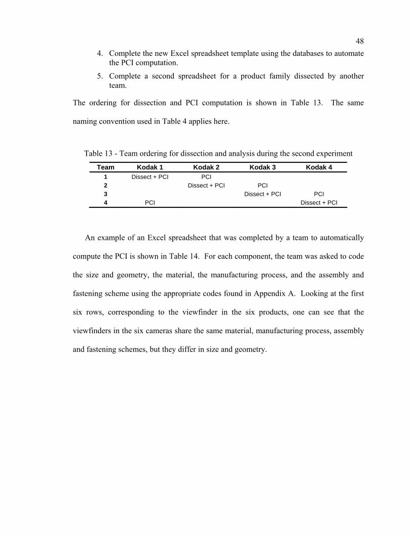
484. Complete the new Excel spreadsheet template using the databases to automate

the PCI computation.

5. Complete a second spreadsheet for a product family dissected by another team.

The ordering for dissection and PCI computation is shown in Table 13. The same

naming convention used in Table 4 applies here.

Table 13 - Team ordering for dissection and analysis during the second experiment

Team Kodak 1 Kodak 2 Kodak 3 Kodak 4 1 Dissect + PCI PCI 2 Dissect + PCI PCI 3 Dissect + PCI PCI 4 PCI Dissect + PCI

An example of an Excel spreadsheet that was completed by a team to automatically

compute the PCI is shown in Table 14. For each component, the team was asked to code

the size and geometry, the material, the manufacturing process, and the assembly and

fastening scheme using the appropriate codes found in Appendix A. Looking at the first

six rows, corresponding to the viewfinder in the six products, one can see that the

viewfinders in the six cameras share the same material, manufacturing process, assembly

and fastening schemes, but they differ in size and geometry.

49Table 14 - Example of spreadsheet for the Kodak family for the second experiment

Component Product Size and Geometry Material Mfg.Process Assembly and

fastening In High Definition 1 3 1 11 In MAX Power Flash 1 3 1 11 In Funsaver 2 3 1 11 In Plus Digital 3 3 1 11 In Waterproof 4 3 1 11

Viewfinder

In Black and White 1 3 1 11 In High Definition 1 3 1 13 In MAX Power Flash 1 3 1 13 In Funsaver 2 3 1 13 In Plus Digital 3 3 1 13 In Waterproof 4 3 1 13

Film Advance Wheel

In Black and White 1 3 1 13

4.3.2. Results from the Second Experiment

Similar to the previous experiment, the PCI values computed by each team for each

family were subject to variation during dissection (omitted or “forgotten” components);

the corresponding results are listed in Table 15. Results of the experiment can be found

in Appendix D.

Table 15 - Initial PCI values for the second experiment

Team Kodak 1 Kodak 2 Kodak 3 Kodak 4 1 62.2 58.5 2 50.2 53.7 3 64.4 63.1 4 50.6 53.4

To analyze the variation due to the components omitted in the analysis, the data were

“corrected” using the same process as in the first experiment. The “corrected” values are

given in Table 16. In the next section, these values are discussed and compared to the

ones obtained in the first experiment.

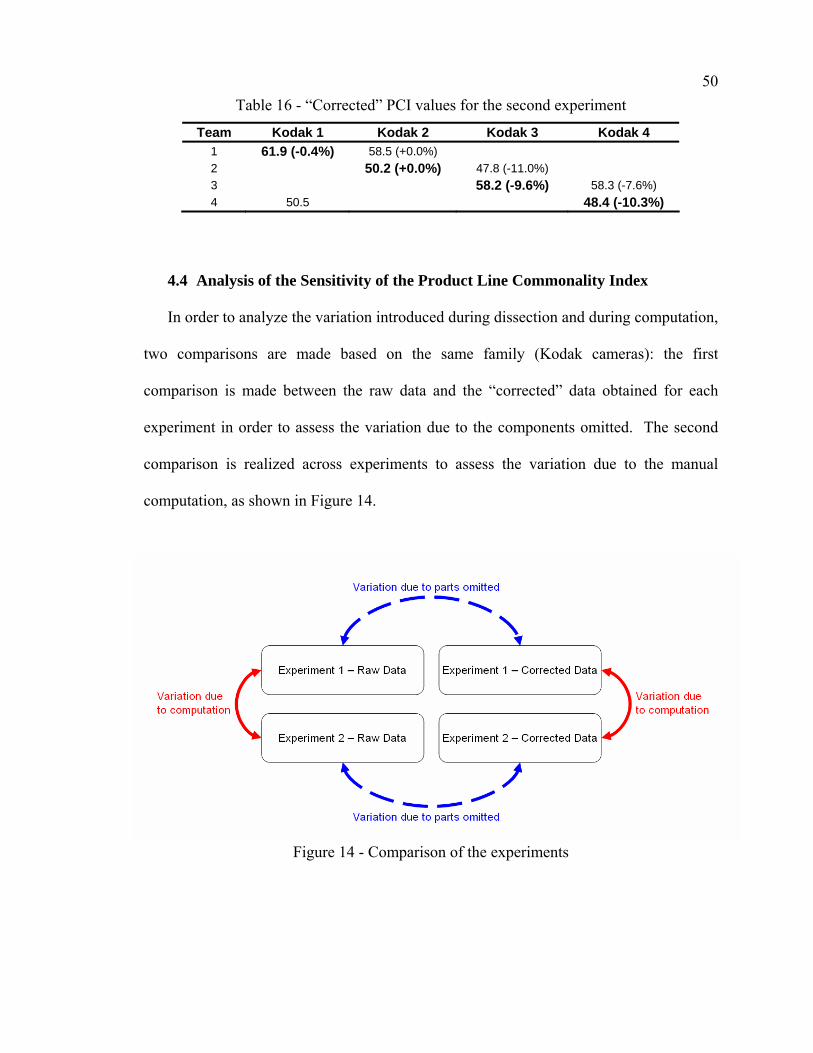
50Table 16 - “Corrected” PCI values for the second experiment

Team Kodak 1 Kodak 2 Kodak 3 Kodak 4 1 61.9 (-0.4%) 58.5 (+0.0%) 2 50.2 (+0.0%) 47.8 (-11.0%) 3 58.2 (-9.6%) 58.3 (-7.6%) 4 50.5 48.4 (-10.3%)

4.4 Analysis of the Sensitivity of the Product Line Commonality Index

In order to analyze the variation introduced during dissection and during computation,

two comparisons are made based on the same family (Kodak cameras): the first

comparison is made between the raw data and the “corrected” data obtained for each

experiment in order to assess the variation due to the components omitted. The second

comparison is realized across experiments to assess the variation due to the manual

computation, as shown in Figure 14.

Figure 14 - Comparison of the experiments

514.4.1. Analysis of the Variation Due to the Components Omitted

As shown in Section 4.2, variation was introduced between groups due to components

that were omitted from the analysis. By “correcting” the data, the components that have

been forgotten are added, hence removing this source of variation. The results can be

found in Table 15. For both experiments, the standard deviation is reduced, from 10.4 to

7.6 in the first experiment (-26.3%) and from 5.8 to 5.5 (-3.8%) in the second experiment.

This source of variation is quite significant and can be easily removed by providing a list

of all the current components during dissection (the dissection is still needed to collect

information regarding each of these components).

Table 17 - Comparison between raw and “corrected” data for both experiments

Raw data (there is variation due to

components omitted)

“Corrected” data (no variation due

to components omitted) Average PCI Standard Deviation Average PCI Standard Deviation Experiment 1 50.8 10.4 53.7 (+5.7%) 7.6 (-26.3%) Experiment 2 57.0 5.8 54.2 (-4.9%) 5.5 (-3.8%)

4.4.2. Analysis of the Variation Due to Computation

To reduce variation even further, the computation phase was automated in the second

experiment. As a result, the standard deviation was dramatically reduced, from 10.4 to

5.8 (-44.2%) when looking at the raw data, and from 7.6 to 5.5 (-28.0%) when looking at

the “corrected” data. This result is even more remarkable when looking at the number of

products and replications of the experiment: while the first experiment only considered 4

products and 4 PCI computations, the second experiment involved more products (6) and

twice as many repetitions (8 PCI computations).

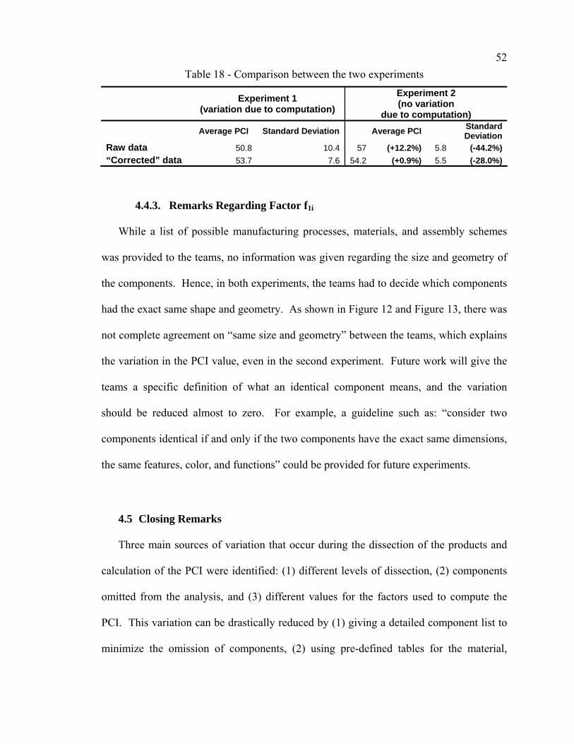
52Table 18 - Comparison between the two experiments

Experiment 1 (variation due to computation)

Experiment 2 (no variation

due to computation)

Average PCI Standard Deviation Average PCI Standard Deviation

Raw data 50.8 10.4 57 (+12.2%) 5.8 (-44.2%) “Corrected” data 53.7 7.6 54.2 (+0.9%) 5.5 (-28.0%)

4.4.3. Remarks Regarding Factor f1i

While a list of possible manufacturing processes, materials, and assembly schemes

was provided to the teams, no information was given regarding the size and geometry of

the components. Hence, in both experiments, the teams had to decide which components

had the exact same shape and geometry. As shown in Figure 12 and Figure 13, there was

not complete agreement on “same size and geometry” between the teams, which explains

the variation in the PCI value, even in the second experiment. Future work will give the

teams a specific definition of what an identical component means, and the variation

should be reduced almost to zero. For example, a guideline such as: “consider two

components identical if and only if the two components have the exact same dimensions,

the same features, color, and functions” could be provided for future experiments.

4.5 Closing Remarks

Three main sources of variation that occur during the dissection of the products and

calculation of the PCI were identified: (1) different levels of dissection, (2) components

omitted from the analysis, and (3) different values for the factors used to compute the

PCI. This variation can be drastically reduced by (1) giving a detailed component list to

minimize the omission of components, (2) using pre-defined tables for the material,

53manufacturing, and assembly schemes, and (3) giving an exact definition of what

identical size and geometry mean. This was validated through the second experiment,

where the standard deviation is reduced. By using these guidelines, the dissection can be

done in a more consistent way, and the collection of data for any component-based

commonality indices used is also more consistent, hence improving the robustness of the

method proposed in Chapter 3. This study was limited to one index, the PCI, which was

the most complex index at the time of the experiment; however, similar experiments can

be conducted for more complex indices that require more information. In the next

chapter, commonality indices to assess the degree of commonality in a product family are

reviewed, and a new index is proposed.

54

CHAPTER 5 COMMONALITY INDICES: ASSESSMENT OF EXISTING

METRICS AND DEVELOPMENT OF A NEW INDEX

5.1 Introduction

The heart of the proposed method is the assessment of the commonality in a product

family. Commonality is best obtained by minimizing the non-value added variation

across the products within a family without limiting the choices for the customers in each

market segment, i.e., make each product within a family distinct in ways customers

notice and identical in ways that customers cannot see. To measure the commonality

within a family of products, several commonality indices have been developed as

discussed in Section 2.1.2. These indices are often the starting point when designing a

new family of products or when analyzing an existing family. They are designed to give

valuable information as to the degree of commonality achieved within the family and

how to improve the design to achieve better commonality in the family and reduce costs.

The goal in this chapter is to develop an appropriate commonality index that can be used

in the proposed method. This is done by first looking at six component-based

commonality indices from the literature to analyze how to use them for product family

benchmarking and redesign. A new commonality index is then introduced to address the

limitations found in the six commonality indices studied. Figure 15 gives an overview of

the chapter.

55

Figure 15 - An overview of the chapter’s goals

First, the relationships between product design and the resulting degree of

commonality within a product family using the six commonality indices (described in

Section 2.1.2) are investigated. Eight different product families are selected and

dissected (see Section 5.2.1), and product information is collected. The commonality

indices are then computed (see Section 5.2.2) and contrasted (see Section 5.2.3) using

four experimental measures: consistency, sensitivity, repeatability and ease of data

collection. These measures are essential when developing the method to support product

family redesign using these indices, and similar criteria are employed by Gershenson, et

56al. [26] in developing their framework for modular product design. While these indices

can give useful recommendation for product family redesign, they have some limitations

(see Section 5.2.4). In order to address these limitations, a new commonality index is

introduced, the Comprehensive Metric for Commonality (see Section 5.3), that is

compared to the six previously described commonality indices (see Section 5.4). Finally,

conclusions are given in Section 5.5.

5.2 A Detailed Comparison of Commonality Indices

This section summarizes the work that has been extensively developed in Refs.

[38,39,67]. The six commonality indices described in Chapter 2 are analyzed.

5.2.1. Dissection of the Products in Each Family and Data Collection

Eight different families of products classified in four groups - one-time-use cameras,

computer mice, power tools, and coffeemakers - are dissected and analyzed for this study

(see Table 19).

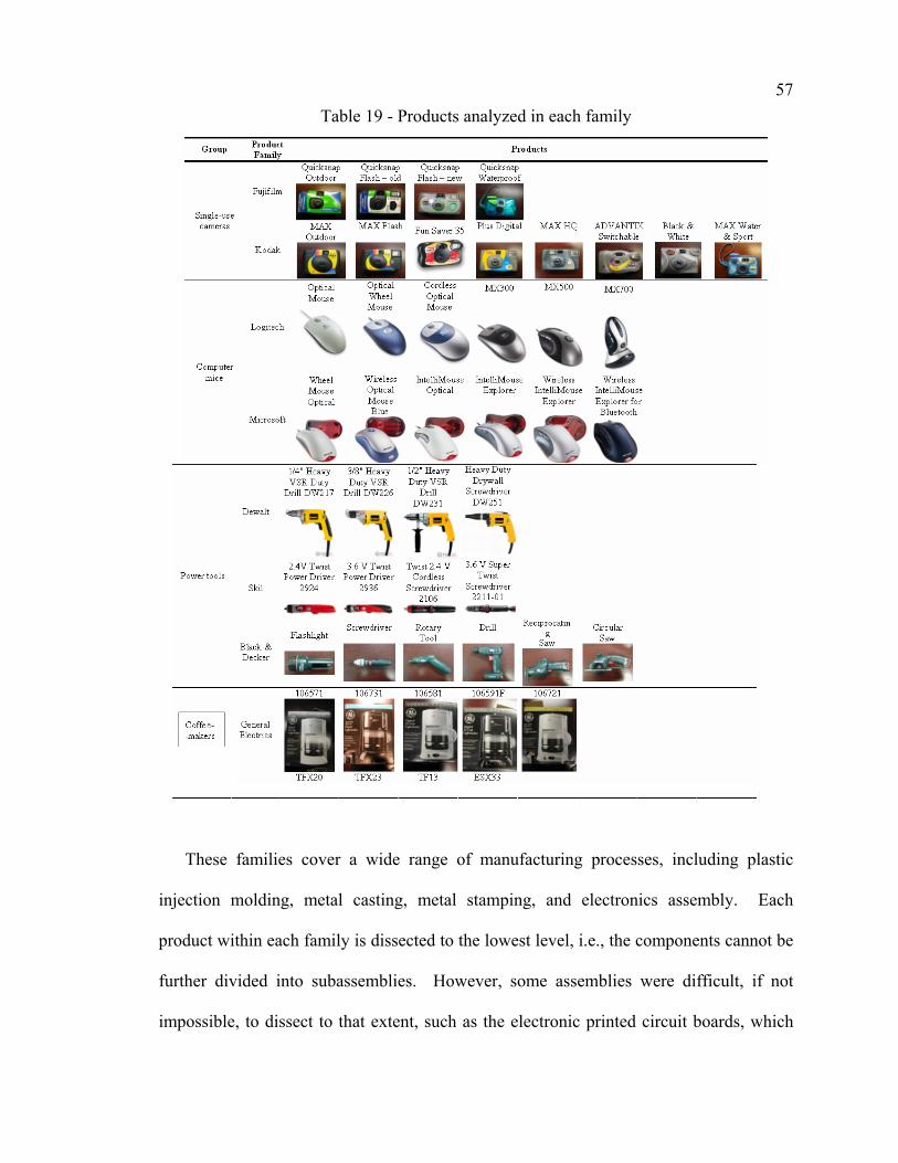
57Table 19 - Products analyzed in each family

These families cover a wide range of manufacturing processes, including plastic

injection molding, metal casting, metal stamping, and electronics assembly. Each

product within each family is dissected to the lowest level, i.e., the components cannot be

further divided into subassemblies. However, some assemblies were difficult, if not

impossible, to dissect to that extent, such as the electronic printed circuit boards, which

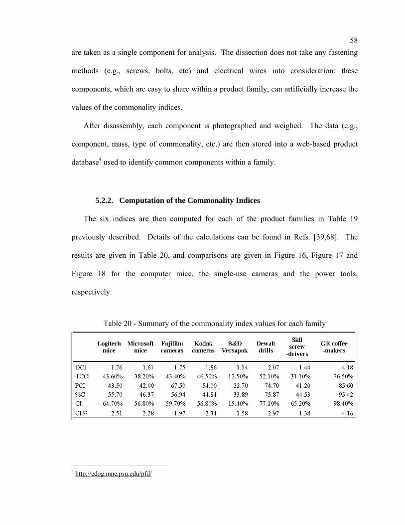
58are taken as a single component for analysis. The dissection does not take any fastening

methods (e.g., screws, bolts, etc) and electrical wires into consideration: these

components, which are easy to share within a product family, can artificially increase the

values of the commonality indices.

After disassembly, each component is photographed and weighed. The data (e.g.,

component, mass, type of commonality, etc.) are then stored into a web-based product

database4 used to identify common components within a family.

5.2.2. Computation of the Commonality Indices

The six indices are then computed for each of the product families in Table 19

previously described. Details of the calculations can be found in Refs. [39,68]. The

results are given in Table 20, and comparisons are given in Figure 16, Figure 17 and

Figure 18 for the computer mice, the single-use cameras and the power tools,

respectively.

Table 20 - Summary of the commonality index values for each family

4 http://edog.mne.psu.edu/pfd/

59

Figure 16 - Comparison for the computer mice

Figure 17 - Comparison for the single-use cameras

Figure 18 - Comparison for the power tools

5.2.3. Analysis and Comparison of the Commonality Indices

The six commonality indices are now compared based on their consistency (across

and within product families), sensitivity, repeatability and ease of data collection.

60

Consistency of the commonality indices

While the lowest values are for the Black & Decker Versapak family, the highest

values are obtained for the General Electrics (GE) Coffeemakers. These indices are

based on the component viewpoint, and the Black & Decker Versapak products share

almost no common components in the family while the GE coffeemakers share most of

their components. All the other families have commonality indices ranging between

these two extremes.

Although the same trend is observed for all of the indices, two important differences

are observed. First, the PCI for the Fujifilm, the Black & Decker, and the Dewalt

families are much higher than the TCCI and DCI values. In the Fujifilm family, the

commonality is affected by the Quicksnap Flash (new model), whose platform differs

from the three other cameras; in the Black & Decker family, most components are unique

due to the different design of each product; and in the Dewalt family, the commonality is

affected by the presence of one screwdriver, which differs from the other products (three

drills). While computing the PCI, most of the components of these products are not

considered (unique components are removed), and the resulting commonality measure

increases. The second interesting difference is the low CI(C) for the Skil family (1.38),

which is explained by the costs of the non-common components in this family: these

components are expensive to produce, lowering its CI(C) value. For more detail, refer to

Ref. [67].

61Sensitivity Analysis

The commonality indices are subject to two types of variation: (1) variation that is

voluntarily introduced by the user (such as a comparison of two slightly different designs

within a product family) and (2) variation that is involuntarily introduced in the

computation (referred to as “noise”). In order to perform well, the indices should have

two distinct and opposite behaviors regarding these variations: they should detect small

changes in the design voluntarily introduced by the user (accuracy), while not being

sensitive to noise (robustness). In the study conducted in Ref. [38], the effect of the noise

on two commonality indices (the PCI and the CI(C)) is investigated by using Monte Carlo

simulation.

The main conclusion of this analysis is that the commonality indices are insensitive to

small variation in the input factors (i.e., to noise). For example, while the fi factors have

distributions with a large standard deviation (20% of the mean and more), the

corresponding PCI values for all the families have a small standard deviation (between

2.2% and 3.8% of the corresponding mean). Similarly, with a standard deviation of the

inputs up to 25% of the corresponding values, the CI(C) keeps a low standard deviation,

namely less than 3% of the mean.

Repeatability Analysis and Ease of Data Collection

Based on the experiment described in Chapter 4, and on the extensive study found in

Refs. [38,39,67], the repeatability and the ease of data collection can be plotted for each

index, as shown in Figure 19.

62

Figure 19 - Repeatability and ease of data collection of the indices

The easiest indices to compute are the DCI, TCCI and CI as they require the same

amount of information: the components in each product as well as the quantity of each

component. These data can be readily obtained from a Bill of Materials, and the

computation can be easily automated, making these indices highly repeatable. The PCI

and the %C are more difficult to compute, making then less repeatable: they require more

‘subjective’ information, which can vary from one person to another (e.g., the factors fi

for the PCI, as described in Chapter 4). For example, when trying to compare two

components to see if they are common, are components with the same shape, size but a

different material still considered common? Moreover, the %C requires more

computation (one for each product in the family, as opposed to one for the whole family

for the other indices). Finally, the CI(C) computation can be straightforward and

repeatable (if cost data are available), but it can also be the most difficult to compute if

component costs have to be estimated.

635.2.4. Limitation of the Current Indices

While these indices were proven to provide valuable information during product

family redesign [67], they do not fully evaluate the impact of each component within a

product family on the degree of commonality within the family. For example, the CI,

TCCI, and DCI only consider the list of components of each product and compare them

to see if they are common, variant and/or unique. They do not consider critical

information such as component costs, production volume, materials, manufacturing

processes, and assembly, and hence do not completely capture the effect of each

component on the level of commonality in a product family. Another example, the CI(C),

does not look at material, manufacturing processes, or assembly. Another limitation of

theses indices is that they do not fully consider the desired variety in a product family. In

other words, these indices can only reach their “perfect” value for commonality when all

the parameters are common between all the components in all the products in a product

family, regardless of whether these components are adding desired variety to the product

family or not. Only the PCI does not penalize the unique components that provide

specific differentiating functions for a product, but it still penalizes the remaining

components, including the ones that should remain variant in a product or a particular set

of products. Consequently, there is a need for a new metric that assesses the effect of

each component of the overall level of commonality in the product family with more

accuracy. The Comprehensive Metric for Commonality (CMC) introduced in the next

section integrates various aspects of the aforementioned indices into a single measure to

capture more information for each component to assess the impact of each component on

the overall level of commonality and diversity in the product family.

645.3 A New Commonality Metric: the Comprehensive Metric for Commonality

The Comprehensive Metric of Commonality (CMC) can be considered as an

extension of the PCI [41] in order to include production volume and costs, and the

commonality/diversity aspect of each component. The required data and the details of its

computation are discussed next.

5.3.1. Definition of the CMC

Data for the CMC

The CMC is a component-based commonality index, and the following information is

needed for each component in each product in the product family being analyzed:

- manufacturing process;

- material;

- assembly scheme;

- production volume;

- initial cost (e.g., cost of producing a mold for an injection plastic process).

For each product, the information required is:

- a list of components and associated information described above;

- the number of components used in each product;

- the estimated number or products manufactured over the lifetime of the product.

Finally, a cost per unit volume is needed for the different materials that are used. To help

the designer choose the manufacturing process, materials, and assembly process, a list of

possible choices can be given to the designer (see Appendix A). The CMC may first

appear to be more information-intensive than other indices; however, its formulation

makes it more flexible, and if some of the previously mentioned data are not available,

the index can be adapted to use whatever is available. Moreover, the index can be used at

65different levels of granularity: in this dissertation, the CMC is computed at the

component level, but if the number of components becomes too large, the CMC can be

computed at the module level, where each module is considered as a single entity rather

than multiple components.

Differentiating components

Components can be classified as either being differentiating or non-differentiating [41].

Differentiating components are ones that are external (used to differentiate the products

aesthetically) or that provide unique functions for the product. For example, when

considering a family of one-time-use cameras, the identification label (aesthetic

differentiation, see Figure 20a) and the APS film (functional differentiation, see Figure

20b) are differentiating components. On the other hand, the non-differentiating

components are not used to differentiate products, neither aesthetically nor functionally.

As an example, the flash is a non-differentiating component in the one-time-use camera

family (see Figure 20c). All of the unique components are considered to be

differentiating; the common components are non-differentiating, and the variant

components could be either differentiating or non-differentiating. Before computing the

CMC, the first task is to define which components can be made common and/or variant

based on whether or not they are differentiating or non-differentiating components. This

is referred to later as the Redesign Strategy, and it is determined internally by the

company based on the products’ specifications. Each company may have a very specific

and different redesign strategy: some companies may want to focus on commonality and

minimize the differences between the products, while others may prefer to develop

66specific products for small market niches at the expense of commonality. In any case, the

specific redesign strategy is included in the computation of the CMC to accurately reflect

how well the product family is currently designed compared to the goal of the company.

(a) Identification label, differentiating component

(aesthetically)

(b) APS film, differentiating component

(functionally)

(c) Flash, non differentiating

component

Figure 20 - Example of differentiating and non-differentiating components

Formulation

The CMC is defined as:

∑

∑

=

=

−

−= P

iiiiiiii

P

iiiiiiii

CCffffn

CCffffnCMC

1

minmaxmax4

max3

max2

max1

1

max4321

)(****

)(*****

(11)

where:

P = Total number of components. ni = Number of products in the product family that have component i. f1i =Ratio of the greatest number of models that share component i with identical

size and shape to the number of models that have component i (ni). f2i = Ratio of the greatest number of models that share component i with identical

materials to the number of models that have component i (ni). f3i = Ratio of the greatest number of models that share component i with identical

manufacturing processes to the number of models that have component i (ni). f4i = Ratio of the greatest number of models that share component i with identical assembly and fastening schemes to the number of models that have

component i (ni).

67f1i

max = Ratio of the greatest number of models that share component i with identical size and shape to the greatest possible number of models that could have shared component i with identical size and shape schemes.

f2imax = Ratio of the greatest number of models that share component i with

identical materials to the greatest possible number of models that could have shared component i with identical materials.

f3imax = Ratio of the greatest number of models that share component i with

identical manufacturing processes to the greatest possible number of models that could have shared component i with identical manufacturing processes.

f4imax = Ratio of the greatest number of models that share component i with

identical assembly and fastening schemes to the greatest possible number of models that could have shared component i with identical assembly and fastening schemes.

Ci = Current total cost for component i.

∑=

=in

jiji CC

1

Cij = Total cost for component i variant j. ijijij cQC *=

Qij = Quantity of component i variant j. cij = Unit cost for component i variant j. Ci

min = Minimum total cost for component i (obtained when the component is common between all the products having component i).

∑=

=in

jiji CC

1

minmin

Cimax = Maximum total component cost (obtained when the component is variant

in each of the products having component i).

∑=

=in

jiji CC

1

maxmax (computed by taking the most expensive variant available and

the most expensive materials).

For cij, two costs estimates are used.

(1) For the components produced in-house, cij is given by:

ij

bija

ijij Qc

cc += (12)

where: aijc = Material and processing cost (further estimated using component volume *

material and processing cost per unit volume). bijc = Setup cost (for example, for plastic injection components, this will be the

cost to produce the mold).

68 (2) For the purchased components, an appropriate cost estimate should be used for

cij, with decreasing costs as quantity increases due to volume discounts.

The cost estimates used in the dissertation can be refined using more complex cost

models or the current component costs; theses values do not affect the computation of the

CMC. The CMC weights the components in the products depending upon their costs, as

well as their size and geometry, their material, their manufacturing process, and their

assembly process. The CMC ranges from 0 to 1. The highest value of the CMC (=1) is

obtained when all the non-differentiating components are common between all the

products, and they use the cheapest variant available. The lowest value of the index (=0)

is obtained when all the components are different (size, geometry, manufacturing process,

assembly, material) between all the products.

Impact of each component on the CMC

The CMC classifies the different components based on their costs Ci and their factors

fji. The total cost to produce a component i ranges from Cimin to Ci

max, with Cimin being

the lowest cost achievable (best commonality) and Cimax being the most expensive cost

possible (worst commonality).

Table 21 shows the effect of each component on the CMC based on its type

(common, variant, unique, non-differentiating, differentiating), illustrated by an example

from a one-time-use camera family. First, a component k that is common between all the

products using it is considered “ideal”, and there is no need for improvement. In Table

21, the cam is shared between the four cameras, and this is a non-differentiating element.

The corresponding cost Ck is the lowest that can be achieved (called Ckmin): the

69corresponding factors fjk take the highest value, i.e., 1. A variant component l that is

differentiating needs to remain variant, and hence, there is no need for improvement, e.g.,

the front identification label is made different between the four cameras to differentiate

them. The corresponding cost Cl is the lowest that can be achieved (called Clmin); the

factors take the highest value, i.e., fjlmax, but in this case they are less than one. A variant

component m that is non-differentiating between the products is not “ideal”, and hence

penalizes the CMC. As an example, the shutter base has two variants, but this component

does not differentiate the products. The current cost Cm is higher than the minimum cost

achievable Cmmin, and Cm can reach the highest value possible (Cm

max) when all the

products having this component are different (size, geometry, material, manufacturing

process, assembly schemes). In this case, the factors fjm are lower than fjmmax, indicating

that there is room for improvement. Finally, a component n that is unique is considered

non-differentiating and does not penalize the CMC. The waterproof housing is a function

specific to only one camera. The corresponding Cn takes the lowest value (Cnmin), while

the factors fjn takes the highest value (fjnmax). As a summary, the CMC penalizes only the

components that should ideally be common in a product family - the desired variety

added by differentiating components is not penalized.

70Table 21 - Impact of different component types on the CMC

5.3.2. Comparison of the CMC with other Commonality Indices

The different parameters considered in the CMC are listed in Table 22. The CMC

assesses each component of a product family more comprehensively. The component

costs are related to the production volume, the material used, the component volume, and

the initial costs. The different variants in geometry, in material, and in manufacturing

processes of each component are analyzed as well. While the other commonality indices

are also based on this information, they do not capture all of it: the DCI, TCCI, CI and

%C fails to capture the size, geometry, manufacturing processes and costs of each

component; the PCI fails to capture the component costs; and the CI(C) does not take the

size, geometry, manufacturing processes into consideration as shown in Table 22.

Moreover, the CMC is the only index that penalizes only non-differentiating components.

By doing so, the maximum value (in this case, 1) can potentially be obtained when all the

non-differentiating components are common, while in the other indices, the maximum

value is obtained when all the components are common between all the products in a

product family, including the differentiating components (except for the PCI that removes

71the unique components, but still penalizes the remaining differentiating components).

The CMC includes most of the data that are used in the six other indices; hence, it

provides a better assessment of the impact of each component on the level of

commonality, as demonstrated in Chapter 7. A detailed comparison of the CMC with

other commonality indices is given next.

Table 22 - Comparison of the commonality indices based on the information used

Computation of other commonality indices

Six commonality indices (DCI, TCCI, PCI, %C, CI, CI(C)) are computed for a stapler

family from PaperPro (see Section 7.1 for more details), as well as for four other product

families: 2 families of computer mice (Logitech and Microsoft, each containing 6

products), and 2 families of one-time-use cameras (Fujifilm with 4 products, and Kodak

with 7 products). Table 23 summarizes the results, which are analyzed following the

table. Additionally, these values are plotted for four families in Figure 21. Details on the

computation of these indices can be found in Ref. [38] and in Appendix E. Five indices

have fixed boundaries, either between 0 and 1 (TCCI, CI, CMC), or between 0 and 100

(PCI, %C), making it easy to compare the values across product families and across

commonality indices. The CI(C) and the DCI, with moving boundaries, are harder to

interpret.

72Table 23 - Commonality indices for five product families

Figure 21 - Comparison of the commonality indices for four product families

For the PaperPro family, the CMC (12.87%) is relatively low compared to the PCI

and %C (45.60 and 54.80, respectively). The reason is that, although some efforts were

made to make some components common between two of the three staplers, these

components are not the most expensive; hence, the costs can still be significantly reduced

(e.g., have the housing, the base and the anvil common between two of the three staplers;

see Section 7.1 for component details). On the other hand, the PCI and the %C are much

higher, as they focus on the material, manufacturing process, assembly, and connections,

which are mostly common across the three products, but these indices fail to capture the

effect of component costs on the commonality. The TCCI, the CI, the CI(C) and the DCI

are quite low as well, due to their focus only on the percentage of common/unique

components in the family.

73In the Logitech and Microsoft families of computer mice, the opposite trend is

observed: the CMC has a higher value than the other indices. Two reasons can be given:

first, both manufacturers did a good job at making expensive components common;

second, they managed to provide commonality in the non-differentiating components

while keeping the differentiating components different. While the same trend is observed

for the other indices, their information is incomplete, being based only on the number of

common components, connections, etc. They also penalize the desired variety, hence

making the ideal value of 1 (or 100) not an optimal commonality (otherwise components

that must remain variant are made common through all the products in the family). The

CI(C) is also lower for the Microsoft family than for the Logitech family (2.51 versus

2.90), while the opposite trend is observed for the CMC (70.90% vs. 65.77%). This is

However, making comparisons between two families using the CI(C) is irrelevant, as this

index does not have fixed boundaries.

For the Fujifilm and Kodak families, an interesting trend is observed: while the PCI,

%C, TCCI and CI are higher for the Fujifilm family than for the Kodak family, the CMC

is lower (53.75% versus 60.51%). In other words, the Fujifilm family may share more

common components, materials, etc., but the Kodak family focuses more on making the

expensive components and the non-differentiating components common. This is also

seen in the CI(C), which is higher for the family 2 (2.81) than for family 1 (1.94), although

a direct comparison is not possible as this index has moving boundaries.

In summary, the CMC gives more comprehensive results, incorporating both

component costs as well as materials, manufacturing process, assembly schemes, and

desired variety/commonality.

745.4 Summary

In this chapter, component-based commonality indices were reviewed, and a new

index was introduced to addresses some of the limitations found in the existing

commonality indices for a more comprehensive assessment of commonality in a product

family. In the next chapter, the optimization algorithm based on this metric is developed.

75

CHAPTER 6 OPTIMIZATION AND REDESIGN RECOMMENDATIONS

FOR PRODUCT FAMILY REDESIGN

6.1. Introduction

A systematic and consistent method for product family redesign using a genetic

algorithm (GA) is introduced in this research. The idea is to use the Comprehensive

Metric for Commonality (CMC) introduced in the previous chapter to (1) assess the level

of commonality in a given product family, and (2) provide recommendations for its

redesign by maximizing the value of the CMC. In this chapter, Phases 3 and 4 of the

method proposed in Chapter 3 are described, and a new GA-based formulation to support

component redesign within a product family is proposed. After collecting the appropriate

data (Phase 1, see Chapter 4), the assessment of the product family is done using the

Comprehensive Metric for Commonality (Phase 2, see Chapter 2). A GA is then

employed to maximize the CMC subject to specific constraints (Phase 3, see Section 6.2).

The results are then analyzed to provide recommendations (1) at the component-level and

(2) at the product family-level (Phase 4, see Section 6.3). Conclusions are given in

Section 6.4.

6.2. Phase 3: Optimization

In this work, a Genetic Algorithm (GA) is used to maximize the CMC. GAs are

adaptive stochastic optimization algorithms involving search and optimization (see

Section 2.2 for more detail). In this research, each attribute of a component is encoded as

an integer, which is later converted into a binary representation for the GA. The

76algorithm maximizes the CMC, subject to the following additional constraints to facilitate

the selection of components to be redesigned.

Constraint 1: External/differentiating components. The components that are external

on a product usually differentiate the product; these components should not be modified

during redesign. For example, in a family of computer mice, the button shown in Figure

22 should not be modified since it differentiates each mouse.

Figure 22 - Example of differentiating components

Constraint 2: The components that are unique to one product will not be modified.

The unique components provide a specific function that is present in only one product.

These components are used to keep each product different aesthetically and functionally.

Hence, it is desired not to modify these unique components.

Constraint 3: If a component is already common throughout the whole family, the

optimizer should not modify the component. The degree of commonality within a

product family only is considered here. Other parameters, such as the performance of

each product, are not considered. Hence, the components that are common through the

whole are considered ‘best’ for the commonality and should not be modified, although

the individual performance of each product may not be optimized.

77Constraint 4: Maximum number of attributes allowed to change. There is a

restriction on the number of parameters to change between the original design and the

redesigned family. If this constraint is not added, the optimizer will find the “best”

commonality when all the components are common. By adding this constraint, the

designer specifies a maximum number of allowable changes. Hence the algorithm

provides recommendations that most influence the commonality, helping the designer

focus on the critical components to redesign. There are currently no guidelines to choose

the appropriate value for this constraint; however, designers may want to specify a

percentage of the total number of parameters for this constraint.

Based on these four constraints, the design variables are chosen: only the non-

differentiating components are considered. Within this set of components, four attributes

are considered: (1) size and geometry, (2) material, (3) manufacturing process, and (4)

assembly. For a given component, if an attribute is common between all the products

using this component, then this attribute is not considered during optimization.

The mathematical formulation of the problem is shown in Eq. 13:

Maximize CMC

Subject to { }ijklijk VC ∈

i = 1..p j = 1..n k = 1..4

(13)

where: Cijk = value of parameter k for component i in product j.

initialijkC = initial value of parameter k for component i in product j.

Vl = possible value l. { }ijklV = set of possible values allowed for parameter k for component i in product j.

p = total number of components in all the products in the product family. n = total number of products in the product family.

78m = maximum number of parameters allowed to change.

if and 1 otherwise.

To understand the formulation, the parameters are represented in Table 24. For a

given product family with n products, a list of p components is established. For each

component i in each product j, four parameters are considered: Cij1, Cij2, Cij3 and Cij4,

respectively corresponding to the values for Size and Geometry, Manufacturing Process,

Materials and Assembly. The algorithm maximizes the CMC by modifying the values of

these Cijk under the constraint specified above (i.e., the Cijk can take a particular set of

values { }ijklV out of all the possible values Vl).

Table 24 - Definition of the parameters for the GA

Size and geometry ..... k ..... Assembly

in Product 1 C111 ..... ..... ..... C114 in Product 2 C121 ..... ..... ..... C124 .....

.....

.....

.....

.....

.....

in Product j C1j1 ..... ..... ..... C1j4 .....

.....

.....

.....

.....

.....

Component 1

in Product n C1n1 ..... ..... ..... C1n4 .....

.....

.....

.....

.....

.....

.....

in Product 1 Ci11 ..... ..... ..... Ci14 in Product 2 Ci21 ..... ..... ..... Ci24 .....

.....

.....

.....

.....

.....

in Product j Cij1 ..... Cijk ..... Cij4 .....

.....

.....

.....

.....

.....

Component i

in Product n Cin1 ..... ..... ..... Cin4 .....

.....

.....

.....

.....

.....

.....

in Product 1 Cp11 ..... ..... ..... Cp14 in Product 2 Cp21 ..... ..... ..... Cp24 .....

..... ..... ..... .....

.....

in Product j Cpj1 ..... ..... ..... Cpj4 .....

..... ..... ..... .....

.....

Component p

in Product n Cpn1 ..... ..... ..... Cpn4

79The implementation is done in Microsoft Excel, using a dedicated plug-in developed

by Pi Blue, namely, OptWorks Excel5.

6.3. Phase 4: Data Output and Redesign Recommendations

Once the optimization is complete, the optimizer proposes a redesign sequence that

can be compared to the original redesign. Two main types of information are given using

the algorithm: (1) at the product family level, if there exists more than one design for a

particular family, then the algorithm assesses each design and classifies it; (2) at the

component level, a list of components to redesign is proposed to achieve the highest

commonality for a given number of changes.

Recommendations at the product family level: If the designer wishes to assess more

than one design for a product family, the algorithm is also run without the fourth

constraint proposed in Section 6.2 (i.e, no limitation on the number of changes in the

parameters); hence, once the design is optimized, the “ideal” commonality is reached,

i.e., all non-differentiating components are made common in the product family. An

offline analysis of the values obtained after optimization enables the assessment of the

different design strategies. To do so, a graph similar to the ones shown in Figure 23 is

plotted. This graph aims at evaluating different design strategies for the given product

family, based on how the factors that are changed influence the commonality value. By

looking at a simple example (see Table 25), consider a product family consisting of three

products, each product having two components. In this particular example, the

commonality assessment is done using the PCI example for ease of understanding, and

5 http://www.piblue.com/products/optworks_ex.html

80only one parameter is represented. For a particular component, if two products have the

same number, then they share the same component. For example, Component 1 is

different in the three products of Design Strategy 1, while Component 1 has only two

variants in Design Strategy 2, one being shared between Product 1 and Product 2.

Table 25 - Three different design strategies for two components in a product family

Design

Strategy 1 Design

Strategy 2 Design

Strategy 3 in Product 1 1 1 1 in Product 2 2 1 1 Component 1 in Product 3 3 2 1 in Product 1 1 1 1 in Product 2 2 2 1 Component 2 in Product 3 3 1 1

Commonality

Each component is used in each product. Two different design strategies need to be

assessed. In Design Strategy 1 (DS1), the two components are variant in each product

(i.e., no commonality). This is represented by attributing three different numbers to each

component, one for each product (1, 2 and 3). In Design Strategy 2 (DS2), there are two

variants for each component, one variant being used by two products (some level of

commonality), represented by having the same number for Component 1 – Product 1 and

Component1Product 2, and Component2Product 1 and Component2Product 3. The best design

(relative to the concerned commonality indices, in this case the PCI) with the minimum

number of changes is achieved through Design Strategy 3 (DS3): the components are

common between all the products in the family (complete commonality; in fact, the three

81products are identical with regard to these two components). Figure 23 shows the graph

in five different cases: the initial commonality assessment of the two design strategies

(Figure 23a), as well as the maximum commonality value obtained with one, two, three

and four changes allowed (Figure 23b, Figure 23c, Figure 23d and Figure 23e,

respectively).

(a) Initial commonality assessment

(b) Maximum commonality after one change allowed

(c) Maximum commonality after two changes allowed

(d) Maximum commonality after three changes allowed

(e) Maximum commonality after four changes allowed

Figure 23 - PCI versus number of changes in Design Strategies 1 and 2

82By running the GA without the fourth constraint on DS1 and DS2, the optimal value

of the PCI is the one obtained in DS3 (complete commonality). This value will be

identical for both designs, as shown in Figure 23e; however, the minimum number of

changes to achieve this complete commonality is different. In DS1, a minimum of four

changes are necessary to achieve DS3, while only two changes are required in DS2, as

shown in Figure 23e and in Figure 23c, respectively. For any number of changes, the

PCI in DS2 is higher or equal to the one in DS1. Hence, DS1 is a “dominated” design

relative to the PCI: DS2 achieves higher PCI (hence higher commonality) than DS1, for

any given number of changes. The same graph can be plotted for any other commonality

metric previously described, including the CMC.

Recommendations at the component level: The algorithm provides a set of possible

changes that could be implemented to maximize the commonality of the product family

(maximization of the commonality index) for a given number of changes. In this case,

the fourth constraint explained in the previous section is implemented, and the best

combination of components to redesign is obtained. By looking at the example shown in

Table 25 for DS2, with a maximum number of changes set to two, the algorithm returns

the following recommendation:

(1) Change Component 1Product 3 from variant 2 to variant 1,

(2) Change Component 2Product 2 from variant 2 to variant 1.

This results in a PCI of 100. Although this example is trivial, the same method can be

applied on much larger-scale problems, helping the designer focus on the critical

parameters of the critical components to redesign.

836.4. Summary

In this chapter, a new GA-based formulation to support component redesign within a

product family was introduced. The combined use of a genetic algorithm and the

Comprehensive Metric for Commonality to support product family redesign provides

useful information for the redesign of a product family, both at the product family level

(assessment of the overall design of a product family) and at the component level (which

components to redesign, how to redesign them). The reduction of the redesign space by

providing a ranked list of components to modify during product family redesign helps the

designer focus on critical components that he/she may not have easily identified without

such a systematic approach. To validate the proposed method, two example applications

are presented in the next chapter.

84

CHAPTER 7 PRODUCT FAMILY REDESIGN: TWO EXAMPLES

In this chapter, the proposed method introduced in Chapter 3 is validated using two

example applications: a set of staplers from PaperPro (see Section 7.1), and a set of

valves from Flowserve (see Section 7.2). Each phase of the method is described in detail,

and a discussion on the validity of the results is given in Section 7.3.

7.1. PaperPro Staplers Example

7.1.1. Introduction to the PaperPro Family

The first example consists of a line of three staplers from PaperPro. PaperPro is a

new company that is dedicated to offering innovative solutions to improve desktop

productivity. The three staplers range from a 2-15-sheet capacity model to a 2-60-sheet

capacity model as shown in Table 26.

Table 26 - The stapler family Model 500 1000 2000 Capacity 2-15 sheets 2-20 sheets 2-60 sheets

The three staplers, although having similar designs, share almost no components. In

the future, the company would like to extend their product line; hence, to avoid

component proliferation, the company wishes to redesign their existing product line to

increase commonality in the products as much as possible. Using the method proposed in

85Chapter 3, recommendations are given to redesign the three existing products.

Implementation of the four phases of the method is described next.

7.1.2. Phase 1: Data Collection for the PaperPro Family

The three staplers shown in Table 26 are analyzed. No data were available for this

family; hence, dissection was conducted to gather the necessary data. The dissection was

realized in the Mechanical Engineering Department at Bucknell University as part of a

summer Research Experience for Undergraduate Program [69]. To ensure consistency in

dissection, each product within the family was dissected to the lowest possible level. The

dissected staplers are shown in Figure 24.

Figure 24 - Dissected staplers

86The data collected during dissection are stored in an Excel spreadsheet as shown in

Table 27. The first two columns list the name of the components and the corresponding

product. In the next column, Size and Geometry, the designer enters a number indicating

if the component has the same size and geometry between different products. For

example, for a given component, if two products have the same size and geometry, then

they have the same number. If they use different variants of the component with different

size and geometry, then the number is different in the Size and Geometry column

between different products. If a product does not contain a component, then there is no

number in the corresponding column. For the Material, Manufacturing process,

Assembly and Fastening, a code is entered based on values listed in Appendix A.

Table 27 - Example of data entered for the staplers family

87In Table 27, the Spring Pin is unique, and the Staple Track Advance is variant, with

two different variants, one being shared between the 500 and the 1000. In the last

column, the designer enters the quantity of components used per product.

Another table containing the quantity per product is created (see Table 28), based on

discussion with the stapler manufacturer. This number is an estimate for the production

of each stapler over its lifetime.

Table 28 - Products and production volume

Product Quantity 500 2,000,000

1000 3,750,000 2000 2,500,000

The third table created is for the component cost (see Table 29). The components are

either manufactured in-house, or purchased, using the costs given Section 5.3.1. For the

components manufactured in-house, the initial costs, the mass of the component and the

material cost are entered; for the purchased components, the purchasing price and the

volume discounts are entered, based on discussion with the PaperPro engineers.

The production level for each variant is determined automatically using Table 27 and

Table 28. The size and geometry factor affects the production level, and hence the initial

cost (setup price/total production for this component); the material factor, associated with

the component mass, gives an estimate of the material cost. It is obtained by comparing

with similar parts used in other products in conjunction with the expertise of Paperpro’s

engineers. PaperPro’s products and all associated tools and components are

manufactured in China.

88

Table 29 - Component costs

89

7.1.3. Phase 2: Computation of the CMC

This section details Phase 2, i.e., the computation of the CMC. Two tasks are

accomplished. First, a definition of what can be potentially made common and/or variant

between the products is proposed (redesign strategy). Second, the CMC is computed

based on the data collected during the dissection and on the redesign strategy.

Redesign Strategy

The first task is to define which components can be made common and/or variant

based on whether or not they are differentiating or non-differentiating components. This

is done by examining the current market segmentation grid for the stapler family [4]. As

shown in Figure 25, market segments are plotted horizontally in the grid while price tiers

are plotted vertically; each intersection of a market segment with a price tier constitutes a

market niche that is served by one or more of a company’s products. Based on the given

market segmentations, both the 500 and 1000 models target the same market segment,

and hence a different design is not necessarily required for the two staplers. In the

current design, two different platforms are used for the 500 and 1000 models, as shown in

Figure 26. Since the company still wants to offer two products for this particular market

segment (with different capacities and aesthetic properties), most of the components can

be made common between the 500 and the 1000, including the Anvil, the Base, the Staple

Track, the Left and Right Housing, the Striker, the Lever, the Absorber, and the Recoil

Spring. Currently, only six components are common (see Figure 24). To differentiate

the products, a variant Handle and Spring can be potentially used.

90

Figure 25 - Market segmentation grid for the staplers

Figure 26 - Current design strategy and recommended redesign

While the 2000 model requires a different architecture due to different sheet capacity,

some components can still be made common between the three staplers, namely, the

91

Track Back-Stop, the Track Spring, and the Staple Track Advance. If these potential

recommendations are implemented, then the staplers are produced at the lowest cost that

can be achieved, resulting in a CMC value of 1. On the other hand, if all the components

are variant in each product, then the commonality is the “worst”, resulting in the highest

production costs and a CMC value of 0.

CMC computation

Two tables are created automatically, based on the previous data: the product costs

table (see Table 30) and the CMC table (see Table 31). While the product costs table

summarizes the cost for each component in each product, the CMC table computes the

different terms fji and Ci for each component, as well as the resulting CMC. The process

is done automatically, limiting possible errors during computation and increasing its

repeatability.

Table 30 - Product costs table

For this product family, the computed CMC value is 0.1287, which is rather low on

the 0-1 scale. The reason is because the company’s designers opted to share many

components between the 500 and 1000 models but did not focus on sharing the most

92

expensive components; the costs can be significantly reduced. This is illustrated in Table

31, where the Ci is close to Cimax for most components. Note that for the unique

components (e.g., Housing Pin), Ci = Cimax = Ci

min.

Table 31 - CMC computation table

7.1.4. Phases 3 and 4: Optimization and Redesign Recommendations

Two sets of runs are made, one to evaluate the different parameters for the genetic

algorithm, and one for the analysis of the effect of the individual components on the

commonality of the family (i.e., optimization at the component level).

Determination of the parameters for the GA: Since the parameters for the GA are case-

dependent, the values that give the best results are not known a priori. Before optimizing

the design, the values for four parameters of the GA are determined: i.e., crossover (Pc),

mutation (Pm), maximum number of generations (Gen), and population (Pop). Sizing a

GA population to ensure maximum computational leverage and accurate sampling has

been considered empirically in several studies. Goldberg [59] shows how to set

93

population size in the context of recombinative mixing, disruption, deception, population

diversity, and selective pressure to maximize computational leverage. In the current

study, a low of 50 and a high of 200 as the population size is considered. Mutation

settings obtained from experimental investigation as discussed in the GA literature are

shown in Table 32. For the experiment, the lowest (0.001) and highest value (0.01) of the

recommended mutation rate Pm are chosen.

Table 32 - Commonly used constant settings of the mutation rate Pm in GAs Pm Reference 0.001 De Jong [70] 0.01 Grefensette [71] 0.005-0.01 Shaffer et al. [72]

In the GA literature, the crossover probability (Pc) is recommended to start around a

value of 0.5. The values of 0.4 and 0.6 are chosen as the low and high value for

crossover probability are chosen. After choosing the different values for the GA

(crossover, mutation, population, maximum number of generations), the implementation

is done in Microsoft Excel, using a the dedicated plug-in developed by Pi Blue,

OptWorks Excel. The crossover method is two-point: two points are selected on the

parent strings. Everything between the two points is swapped between the parents,

rendering two children. The problem is formulated choosing the CMC as objective

function, and the design variables are defined as shown in Figure 27 and Figure 28,

respectively.

94

Figure 27 - Problem formulation – objective function

Figure 28 - Problem formulation – design variables

The objective function is to maximize the CMC as shown in Eq. 13 in Chapter 6.

Only the first three constraints proposed in Section 6.4 are taken into account: the results

are used to determine the appropriate parameters for the GA. The sixteen possible

combinations of parameters are tested with different initial values; the highest CMCs

reached for these sixteen combinations are summarized in Table 33. The best results are

obtained with combination 5, 7, 8, 14 and 16, with a CMC value of 1, eight times more

than the original value (0.1287). This value is the ideal value, obtained only when all the

95

non-differentiating components that can be potentially common are shared between all

the products in the product family.

Table 33 - Details of experimental runs of the GA

In addition to the CMC value, two other parameters are considered in the comparison

of these sixteen combinations: the number of generations to converge, and the number of

function calls. Ideally, the highest value for the CMC is desired, while having the

number of function calls and the number of generations to converge be as low as

possible. The comparison of these three parameters (CMC, number of generations to

converge and number of function calls) is summarized in Figure 29. The values are

standardized between 0 and 1, a higher value indicating a better performance. The most

satisfying combination is run 16, which is the run where the highest CMC value is

obtained (=1) with the minimum computation time.

96

Figure 29 - Comparison of the runs

Analysis of the effect of the individual components on the commonality: The GA

parameters are now fixed using combination 16, i.e., Pc=0.6, Pm=0.01, Pop=200 and

Gen=5000. The fourth constraint, i.e., the maximum number of parameters allowed to

change, is now implemented. By specifying the maximum number of changes desired,

the optimizer returns the best CMC that is achieved with this particular number of

changes, as well as the corresponding changes.

For a maximum number of changes equal to six (chosen arbitrarily), the GA returns

the following recommendations for the stapler family:

- make the Anvil common between the 500 and the 1000;

- make the Track Back-Stop common between the three staplers;

- make the Staple Track common between the 500 and the 1000;

- make the Staple Track Advance common between the three staplers;

- make the Left Housing common between the 500 and the 1000; and

- finally, make the Right Housing common between the 500 and the 1000.

97

The feasibility of this solution is ensured by the fact that only feasible changes are

allowed during the optimization phase—the constraints entered take into account the

feasibility of the solutions. For example, the designer does not want to share the anvil

between the 500, 1000, and 2000 models; hence, by adding constraints, the anvil can only

be shared by the 500 and 1000. In a more generic case, these constraints may be relaxed,

but the feasibility of the solutions will not be guaranteed. By implementing the six

recommendations previously described, the CMC increases from 12.87% to 70.72% (an

improvement of 450%); regarding the product costs, they are also significantly reduced

as shown in Table 34 (from -1.90% for the 2000 to -8.38% for the 1000).

Table 34 - Product costs for the stapler family Model 500 1000 2000 Original costs $2.05 $2.46 $4.32 Optimized costs $1.97 $2.26 $4.24 Difference -4.06% -8.38% -1.90%

While the CMC value is increased by almost five times, the corresponding cost

savings are much smaller (at most 8.38%). The reason is because the CMC integrates not

only component costs but also similarity factors. In this case, the similarity factors (fji)

are significantly improved, but the corresponding cost savings do not follow the same

trend. For example, by making the Left Housing common between two of the three

staplers (the 500 and the 1000), the similarity factors (fji) jump from 1/3 to 2/3 (an

increase of 100%), while the corresponding decrease in cost is smaller (-2.10% for the

500 and -12.45% for the 1000).

98

7.1.5. Validation of the Results

To validate the results from the method, discussions with one of the cofounders of

PaperPro, Brian Melgaard, was established. The method was explained to him, as well as

the example previously described. The hypothesis (that he validated) was that the 500 and

the 1000 staplers can share most of their components, as they have similar designs. The

questions that were asked to him are the following:

- For this particular example, do the six recommendations generated by the

algorithm make sense? (i.e., if you have to redesign the three products to

improve commonality and still keep the same specific characteristics for each

stapler, would you start focusing on the six recommendations proposed?)

- If not, which recommendation(s) do(es) not make sense? Why?

- Would you propose any other recommendations to implement before the six

indicated? (i.e., are there any other points that are more critical than the ones

cited if you have to redesign the staplers?

His answers and comments are compiled next. While he agreed that “commonality

between components is very beneficial”, he reckoned that “when designing these staplers,

very little focus was placed on the commonality of the parts”, as “[they] were a 2 person

company, with 0 money, and speed to market was more important than part

commonality”. He agreed that the recommendations provided by the algorithm were

satisfying, as they would have focused on the same components if they had this particular

strategy in mind. Although they are currently trying to adopt another strategy (leverage

the 500, 1000, and 2000 to create high-end “premium” staplers with a different housing

to satisfy more market niches), according to him, the information provided by the

99

algorithm is “helpful as [they] move forward and develop new products”. By helping

them focus on the critical components to make/keep common and variant, the algorithm

also provides useful information for the designers when developing new products.

Having Brian Melgaard confirm the proposed recommendations validates that the

CMC assesses the commonality in the product family. What is important to notice is

that, in this example, the scale of the problem is rather limited (fewer than 15 components

per product and only three products); the use of optimization for such a simple family is

not necessary; however, the same method and metric can be applied to much larger

families with more complex products, which could help designers quickly identify the

components and parameters that most influence the commonality.

Another way to validate the proposed method and the CMC is to run the same method

with five of the previously described indices (the DCI, the TCCI, the PCI, the CI and the

CI(C)) and to compare the proposed recommendations. The same constraints were kept,

as well as the maximum number of changes was equal to six. Four of these indices

weight the components equally; hence, when maximizing their value using the algorithm,

thousands of solutions are returned, with the same maximum value. It is difficult to

identify on which components to focus. The maximum values returned for these four

indices are shown in Table 35.

Table 35 - Comparison of five indices before and after improvement of the family Initial Value Optimized Value Difference DCI 1.16 1.38 +18.53% TCCI 13.95% 27.91% +100.05% PCI 45.6 60.44 +32.54% CI 21.43% 42.86% +99.99%

100

The only direct comparison possible is between the CI(C) and the CMC, as these

indices weigh the components based mainly on component costs. The algorithm returns

the following recommendations for the stapler family when using the CI(C):

- make the Anvil common between the 500 and the 1000;

- make the Base common between the 500 and the 1000;

- make the Staple Track common between the 500 and the 1000;

- make the Handle common between the 500 and the 1000;

- make the Left Housing common between the 500 and the 1000;

- finally, make the Right Housing common between the 500 and the 1000.

Compared to the recommendations obtained with the CMC, only four out of six are

identical. By implementing these six recommendations, the CI(C) increases by 1.85%,

from 1.08 to 1.10. The reason why this increase is relatively low compared to the one

observed in the other indices is the way the index is formulated: first, the CI(C) does not

have fixed boundaries, making comparisons difficult; second, the original design is not

taken into account when computing it. Hence, even if the costs can be dramatically

reduced compared to the original design, the CI(C) does not take this difference into

account, but rather looks at the final cost of each component. By consulting PaperPro’s

cofounder, the recommendations given using the CI(C) are less satisfactory than the ones

returned when using the CMC. These two indices (CMC and CI(C)), focusing both on

costs, tend to put more emphasis on the expensive components. The differences are due

to the fact that the CMC includes more data in the analysis and may consider less

expensive components that are significantly different in shape, materials, etc. As a

conclusion, the CMC was proven to return only one set of recommendations (unlike the

DCI, the TCCI, the PCI and the CI), but also gives recommendations that are closer to

what designers would actually implement. Moreover, by having fixed boundaries, it is

101

easier for designers to understand how good the current design of a product family is and

to see the effect of commonality on cost reduction.

7.2. Flowserve Valves Example

7.2.1. Introduction to the Flowserve Families

The second example used to demonstrate and validate the proposed method is a case

study from Flowserve. The focus is on their valve division. Flowserve recently acquired

two valve manufacturers, namely, Anchor Darling and Edward. In this case study, two

product families from the former Edward company are studied, as shown in Table 36.

Table 36 - Products analyzed Family Piston Check Stop Stop Check

1” 2” 1” 2” 1” 2”

Regular

1” 2” 1” 2” 1” 2”

Univalve

102

Three types of valves were analyzed (Piston Check, Stop and Stop Check) in two

sizes (1” and 2”) from two families: the Regular and the Univalve families. One

particularity of these two families is that, although they offer similar functionalities, their

design and manufacturing processes differ greatly. The differences are due to the way

these product families were designed: the Regular family was developed without taking

commonality into consideration, while the Univalve family, more recent, was designed

with the idea of product family and component sharing in mind. Moreover, although

these two families offer similar functions, they are still both in production. The reason is

that they are not competing directly, as the market is very specific, and consumers want

to replace defective valves with the exact same models: if the consumers bought Regular

valves in the past, they do not want to switch to the Univalve products, and vice versa.

After discussions with engineers from Flowserve, they all agree that the Univalve product

family has a much higher commonality and better design than the Regular product

family, sharing more components. The method previously developed is hence applied to

both product families to analyze the two designs at the component level and as the

product family level. At the component level, the algorithm is applied to the Regular

family, and the recommendations from the algorithm are compared to the current design

of the Univalve family to see if the proposed recommendations for the Regular family

and what has been currently implemented in the Univalve family match. At the product

family level, the commonality is assessed for both families to compare both designs and

see how they can be improved.

103

7.2.2. Phase 1: Data Collection for the Flowserve Families

The data were collected on-site at the Raleigh factory, with the help of Flowserve

engineer Ron Farrell. For each of the twelve products analyzed, a Bill of Materials was

obtained, containing the part name, description, and costs. The additional information

required to compute the CMC was collected by hand. The data were then entered into an

Excel spreadsheet, as shown in Table 37 for the Regular family and in Table 38 for the

Univalve family. For a given component, in both families, the manufacturing process,

the material, and the assembly were identical; the size and geometry was the only factor

that varied. Hence, in both tables, only the “Size and Geometry” factor is represented,

along with the cost of each component.

Table 37 - Data for the Regular family

104

Table 38 - Data for the Univalve family

7.2.3. Phase 2: Computation of the CMC

Two tasks are accomplished during Phase 2, as previously with the stapler family.

First, a definition of what can be potentially made common and/or variant between the

products was proposed (redesign strategy); second, the CMC was computed based on the

data collected during the dissection, and on the redesign strategy.

Redesign Strategy

The first task was to define which components could be made common and/or

variant. After discussion with Flowserve engineers, the size difference between the 1”

and 2” valves were determined to be too different to make most parts common between

105

these two sizes; however, for a given size, components can be made common. Only four

components can be potentially made common between all the products in the family: the

Packing 1, the Packing 2, the Handwheel and the Nameplate. The aesthetical

differentiation is not critical here; hence the external components need not be different.

CMC Computation

Two tables were created automatically based on the data in Table 37 and Table 38.

Two CMC tables were generated, one for each family, as shown in Table 39 and Table

40. The process was done automatically, limiting possible errors during computation and

increasing its repeatability.

Table 39 - CMC computation table for the Regular family

106

Table 40 - CMC computation table for the Univalve family

The CMC for the Regular family is 0.5624, much lower than the value in the

Univalve family (0.8067). This result was anticipated, as the Univalve family has been

designed with more emphasis on component sharing.

7.2.4. Phases 3 and 4: Optimization and Redesign Recommendations

In this section, recommendations are given and validated, at the component level and

at the product family level.

Recommendations at the component level: The algorithm is applied to the Regular

family, and the recommendations from the algorithm are compared to the current design

of the Univalve family, to see if the proposed recommendations for the Regular family

107

and what has been currently implemented in the Univalve family match. The Regular

family has twenty-five components; the Univalve family has thirty components. Out of

these components, seventeen are present in both families, as shown in Table 41.

Table 41 - Comparison of the components between the two valve families

Out of these seventeen components present in both families, eleven have the same

type of variants shared between the products. The remaining six components have a

different “sequence”:

- For the Disk Casting, three variants are used in the Univalve family, compared to

four in the Regular family.

- The Handwheel is common between all the products in the Univalve family that

have the component, while two variants are used in the Regular family.

- The Nut Hex is common between all the products in the Univalve family, while

two variants are used in the Regular family.

108

- There are three Packings 1 in use in the Univalve family, compared to four

Packings 1 in the Regular family.

- There are three Packings 2 in use in the Univalve family, compared to four

Packings 1 in the Regular family.

- There are five Screw Hex in the Univalve family, compared to two Screw Hex in

the Regular family.

Except for the Screw Hex, the Univalve family shares more components between its

products than the Regular family. For each family, the parameters for the GA are

determined, similarly as in the PaperPro example. The same combination of parameters

was found for both families: Pc=0.6, Pm=0.01, Pop=200 and Gen=5000. The algorithm

is then run on the Regular family, using a maximum number of changes arbitrarily set to

five. The set of recommendations proposed by the method is shown in Table 42.

Table 42 - Recommendations with a number of changes equal to five

Component From Product Factor Recommendation Disk Casting Stop 1” f1 3 to 1 Disk Casting Stop 2” f1 4 to 1 Packing 1 Stop Check 1" f1 3 to 1 Packing 1 Stop Check 2" f1 4 to 1 Packing 2 Stop Check 1" f1 3 to 1

The five recommendations concern three components that are in use in both families

of products: the Disk Casting, the Packing 1 and the Packing 2. The algorithm

recommends using only two variants of the Disk Casting, one for the 1” diameter

products (Stop 1”, Stop Check 1” and Piston Check 1”), and one for the 2” diameter

products (Stop 2”, Stop Check 2” and Piston Check 2”), as already implemented in the

Univalve family. The algorithm also recommends reducing the number of variants for

109

Packing 1 and in Packing 2, as observed in the Univalve family. By implementing these

five recommendations, the CMC in the Regular family is improved by 45%, from .5624

to .8163. This value is comparable to the current CMC for the Univalve family (0.8067).

The maximum number of changes is then taken equal to ten. The proposed

recommendations are shown in Table 43.

Table 43 - Recommendations with a number of changes equal to ten

Component From product Factor Recommendation Disk Casting Stop 1” f1 3 to 1 Disk Casting Stop 2” f1 4 to 1 Packing 1 Stop Check 1" f1 3 to 1 Packing 1 Stop Check 2" f1 4 to 1 Packing 2 Stop Check 1" f1 3 to 1 Packing 2 Stop Check 2” f1 4 to 1 Gskt spl wnd Piston Check 1" f1 1 to 2 Gskt slp wnd Stop 1" f1 1 to 2 Handwheel Stop 2" f1 2 to 1 Handwheel Stop Check 2" f1 2 to 1

The first remark is that the five recommendations previously proposed are still

identified by the algorithm and five additional recommendations are given. In these five

additional recommendations, three concern two components that are used in both

families: the Packing 2 and the Handwheel. These three recommendations suggest

making common the Packing 2 among all the products, as well as the Handwheel. The

same strategy was adopted for the Univalve family that already shares a common

Handwheel between the products. Implementing these ten recommendations improves

the CMC for the Regular family from an initial value of .5624 to 0.8993, an

improvement of 60%. The method was validated through this case study, where the

recommendations given from the algorithm match the implementation in the Univalve

family.

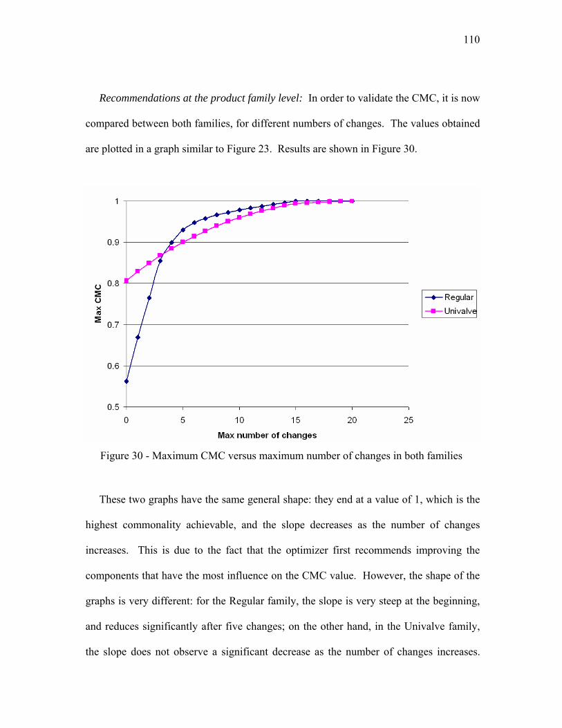
110

Recommendations at the product family level: In order to validate the CMC, it is now

compared between both families, for different numbers of changes. The values obtained

are plotted in a graph similar to Figure 23. Results are shown in Figure 30.

Figure 30 - Maximum CMC versus maximum number of changes in both families

These two graphs have the same general shape: they end at a value of 1, which is the

highest commonality achievable, and the slope decreases as the number of changes

increases. This is due to the fact that the optimizer first recommends improving the

components that have the most influence on the CMC value. However, the shape of the

graphs is very different: for the Regular family, the slope is very steep at the beginning,

and reduces significantly after five changes; on the other hand, in the Univalve family,

the slope does not observe a significant decrease as the number of changes increases.

111

Another main difference is the initial value, lower for the Regular family than for the

Univalve family. The explanation is that in the Univalve family, the components that are

critical for a commonality perspective are already shared between the products, unlike in

the Regular family. Hence, while the initial CMC is lower in the Regular family, the

potential for improvement is greater than for the Univalve family by focusing on

components that strongly affect the commonality. The slope is hence directly related to

the potential commonality improvement in the family. The magnitude of the slope can

be used in future research as a stopping criterion for the optimizer: if the slope is less

than a certain user-defined threshold value, then the optimizer stops as the potential for

improvement is too low for being beneficial to the redesign. Another remark is that,

although there was a common agreement from Flowserve designers on the fact that the

Univalve family had a better design (confirmed with a higher initial CMC value), the

graph shows that the ease of redesign (i.e., the potential gain in commonality) in the

Regular family is higher than in the Univalve family: with more than five changes, the

CMC for the regular family is higher than in the Univalve family. Moreover, the

minimum number of changes to achieve perfect commonality is higher for the Univalve

family than for the Regular family (20 versus 15). This can be explained by the fact that

although the Univalve family was designed with a focus on critical components to make

common (high initial CMC value), designers might have overlooked other components

that could have been easily made common (although they have less influence on the

global commonality), such as the Screw Hex, which has five variants when one would

have been enough for the six products.

112

In conclusion, this graph enables the visualization of the current commonality in a

product family, but also helps identify how easy it is to redesign a family to improve its

commonality. For this particular example, the graph also validates the method, showing

that the Univalve family has a better initial design, which is harder to improve (high

initial CMC, low initial slope) than the Regular family (low initial CMC, higher initial

slope).

7.2.5. Validation of the results

The method was validated through this case study. At the component level, the

recommendations provided by the algorithm on how to improve the Regular family

match what can be found in the Univalve family. At the product family level, the

algorithm provided significant information on not only the current value of the

commonality in both families, but also on how easy it is to redesign the families.

7.3. Scalability of the algorithm

To check the scalability of the algorithm, the run-time and the number of function

calls is also recorded for the optimization of three product families, namely, the

Microsoft mice, the PaperPro staplers and the Fujifilm single-use cameras. Each family

has a different number of parameters that can vary, ranging from 17 for the PaperPro

family to 56 for the Fujifilm family. For each optimization, the same computer was used,

running on an Intel Inside Pentium 4 Hyper Thread Processor at 3.2GHz with 1GB of

RAM. Depending on the maximum number of parameters allowed to change, the run-

time varied between 170s and 480s, as shown in Table 44.

113

Table 44 - GA run-time

The run-time is then plotted against the number of parameters that can vary (see

Figure 31).

Figure 31 - Numbers of parameters that can vary versus GA run-time

114

Notice that the run-time seems to be a linear function of the number of parameters

that can vary. As a consequence, the algorithm implemented may be used for larger-scale

problems with more parameters without significantly increasing the computational time.

7.4. Summary

This chapter demonstrated and validated the proposed method through two case

studies. In the first example, a set of staplers was analyzed, and recommendations were

given on how to redesign them. These recommendations were validated by talking to the

co-founder of the stapler manufacturing company. In a second example, the combined

use of a genetic algorithm and the Comprehensive Metric for Commonality to support

product family redesign provided useful information for the redesign of two families of

valves, both at the product family level (assessment of the overall design of a product

family) and at the component level (which components to redesign, how to redesign

them).

115

CHAPTER 8 CONCLUSIONS AND RECOMMENDATIONS

In this thesis, a systematic and consistent method to provide recommendations during

product family redesign was introduced, demonstrated and validated. This chapter

summarizes the proposed method, its capabilities and its limitations. The chapter

concludes with recommendations for further research involving additional development

and validation of the method.

8.1. Contributions

The main objective in this research was to develop a novel method for product family

redesign and to demonstrate its use. While developing this method, three sub-objectives

were completed. First, a comprehensive metric to assess the commonality in a product

family (Comprehensive Metric for Commonality, CMC) was proposed to address the

limitations of existing component-based commonality indices. Second, guidelines were

proposed to reduce variation when collecting data during product family dissection.

Third, a new GA-based formulation to support component redesign within a product

family was introduced and implemented. The CMC, the guidelines for product

dissection, the new GA-based formulation and the redesign method introduced in this

dissertation are summarized in Sections 8.1.1, 8.1.2, 8.1.3 and 8.1.4 respectively.

8.1.1. The Comprehensive Metric for Commonality

The proposed Comprehensive Metric for Commonality (CMC) is a component-based

commonality index. The CMC was proposed after extensively studying existing

116

component based commonality indices. The CMC helps the designer resolve the tradeoff

between too much variety and too much commonality by penalizing only the components

that should ideally be common, given the product mix. It includes the following

parameters at the component level: size, geometry, material, manufacturing process,

assembly, and costs. This index was proposed to address the limitations found in the

current component-based commonality indices. The CMC was applied to two case

studies in Chapter 7, and the method provided an effective assessment of the design of a

product family.

8.1.2. Guidelines for Product Family Dissection

A set of guidelines on how to dissect a product family was created, aiming at

minimizing variation due to involuntary input variation (“noise”) when computing

commonality indices in order to yield more consistent results. This variation can be

drastically reduced by (1) giving a detailed component list to minimize the omission of

components, (2) use pre-defined tables for the material, manufacturing, and assembly

schemes and (3) give an exact definition of the different terms used in the commonality

indices. The proposed guidelines were validated through two experiments. By using

these guidelines, the dissection can be done in a more consistent way, and the collection

of data for any component-based commonality indices used is also more consistent,

hence improving the robustness of the method summarized in Section 8.1.4.

8.1.3. GA-Based Formulation to Support Component Redesign

A new formulation to support component redesign using a genetic algorithm was

introduced. Four parameters (size and geometry, materials, manufacturing process, and

117

assembly) are used for each component in each product to assess the design of a product

family by computing and maximizing the CMC. This formulation also includes the

specifications of constraints on these parameters based on the redesign strategy for the

product family. This novel approach captures the commonality of a product family at the

component level as well as the desired commonality and variety in the family.

8.1.4. Method for Product Family Redesign

The proposed method provides systematic and consistent results and

recommendations to help redesign an existing product family. Using simple data as

inputs (a list of components in each product with related information, obtained directly

from a Bill of Materials and/or from the dissection of the product family using the

proposed guidelines), as well as the redesign strategy (which component to keep

common, variant, etc.), the method first assesses the design of a family using the

Comprehensive Metric for Commonality. A genetic algorithm is then employed to

maximize the commonality of the entire family without penalizing the desired variety.

The combined use of a genetic algorithm and the Comprehensive Metric for

Commonality provides useful information for the redesign of a product family, both at

the product family level (assessment of the overall design of a product family) and at the

component level (which components to redesign, how to redesign them). The method

was demonstrated and validated through two case studies in Chapter 7, providing

significant information for the designer during product family redesign.

118

8.2. Recommendations for Future Research

Regarding The Comprehensive Metric for Commonality: While the proposed CMC

captures more data than other indices, making the assessment of a product family more

thorough, it does not take into account component performance, and hence the tradeoff

between product performance and commonality is not captured. Future work suggests

including more data in the CMC, particularly related to the performance and the

functionalities of the components.

Regarding the Proposed Guidelines for Product Family Dissection: The work presented

in this dissertation concerns only one commonality index, the PCI, applied to products

with relatively few components (less than 40 components per product). Future work

suggests repeating the experiments on other commonality indices, including the

Comprehensive Metric for Commonality, as well as on a wider array of product families

with more complex products consisting of more components.

Regarding the Proposed Method: Another research direction is the use of multiple

indices to capture the commonality in a product family, but also other parameters, such as

the product performance, etc. The choice of indices should be related to a company’s

design strategy [38]. The proposed method can also be extended for product family

design (i.e., new product development) to support decision at every stage of the product

design process. In the long-term, the method should be included as part of a framework

to (1) capture existing information on a product family, (2) retrieve and (3) reuse this

information for product family and product platform design at every stage of a product

development.

119

Regarding Product Family Design and Redesign: This research addresses some issues

found today in product family redesign. Other research directions are, but not limited to:

- Product platforms: How to quantify the benefits of product platforming? How can a

platform be designed to accommodate future technologies? How to design a product

platform and manage uncertainties?

- Information management for product family: how to capture, retrieve and reuse

information for product family design? How to propagate changes in a product family?

- Product variety: what is the effect of product variety on the market? How to provide

variety? When does variety bring value?

8.3. Summary

As more manufacturing companies seek to benchmark, redesign and consolidate their

product lines, there is an increased need for more systematic and consistent approaches to

product family redesign that are useful during concept development and layout design.

To answer this need, this dissertation presented a systematic and consistent method to

help designers during product family redesign. Through two case studies, this method

has provided valuable recommendations to the designer, helping him/her focus on critical

components to provide enough variety to the customers without sacrificing commonality

between the products in a product family. Developing such methods will provide product

family designers with useful recommendations that could be implemented during product

family redesign, which will help reduce manufacturing costs.

120

REFERENCES [1] Siddique, Z., Rosen, D. W. and Wang, N., 1998, "On the Applicability of Product

Variety Design Concepts to Automotive Platform Commonality," ASME Design Engineering Technical Conferences - Design Theory and Methodology, Atlanta, GA, ASME, Paper No. 1998-DETC/DTM-5661.

[2] Pine, B. J., 1993, "Mass Customizing Products and Services," Planning Review, 22(4), pp. 6-13.

[3] McGrath, M. E., 1995, Product Strategy for High-Technology Companies, Irwin Professional Publishing, New York.

[4] Meyer, M. H. and Lehnerd, A. P., 1997, The Power of Product Platforms: Building Value and Cost Leadership, The Free Press, New York.

[5] Collier, D. A., 1980, "Justifying Component Part Standardization," Twelfth National AIDS Conference, Las Vegas, NV, pp. 405.

[6] Collier, D. A., 1981, "The Measurement and Operating Benefits of Component Part Commonality," Decision Sciences, 12(1), pp. 85-96.

[7] Collier, D. A., 1982, "Aggregate Safety Stock Levels and Component Part Commonality," Management Science, 28(11), pp. 1296-1303.

[8] Collier, D. A., 1979, "Planned Work Center Load in a Material Requirements Planning System," Eleventh National AIDS Meeting, New Orleans, LA.

[9] Fisher, M., Ramdas, K. and Ulrich, K., 1999, "Component Sharing in the Management of Product Variety: A Study of Automotive Braking Systems," Management Science, 45(3), pp. 297-315.

[10] Thonemann, U. W. and Brandeau, M. L., 2000, "Optimal Commonality in Component Design," Operation Research, 48(1), pp. 1-19.

[11] Krishnan, V. and Gupta, S., 2001, "Appropriateness and Impact of Platform-Based Product Development," Management Science, 47(1), pp. 52-68.

[12] Lutz, R. A., 1998, Guts: The Seven Laws of Business that Made Chrysler the World's Hottest Car Company, John Wiley, New York, NY.

[13] Simpson, T. W., Seepersad, C. C. and Mistree, F., 2001, "Balancing Commonality and Performance within the Concurrent Design of Multiple Products in a Product Family," Concurrent Engineering: Research and Applications, 9(3), pp. 177-190.

[14] Bremmer, R., 1999, "Cutting-Edge Platforms," Financial Times Automotive World,pp. 30-38.

[15] Wilhelm, B., 1997, "Platform and Modular Concepts at Volkswagen - Their effect on the Assembly Process," Transforming Automobile Assembly: Experience in Automation and Work Organization, Shimokawa, K., Jürgens, U. and Fujimoto, T. eds., Springer, New York, NY, pp. 146-156.

[16] Aboulafia, R., 2000, "Airbus Pulls closer to Boeing," Aerospace America, 38(4), pp. 16-18.

[17] Simpson, T. W., Maier, J. R. A. and Mistree, F., 2001, "Product Platform Design: Method and Application," Research in Engineering Design, 13(1), pp. 2-22.

[18] Sanderson, S. W. and Uzumeri, M., 1997, Managing Product Families, Irwin, Chicago, IL.

[19] Wheelwright, S. C. and Clark, K. B., 1995, Leading Product Development, Free Press, New York, NY.

121

[20] Lehnerd, A. P., 1987, "Revitalizing the Manufacture and Design of Mature Global Products," Technology and Global Industry: Companies and Nations in the World Economy, B. R. Guile and H. Brooks eds., National Academy Press, Washington, D.C., pp. 49-64.

[21] Pessina, M. W. and Renner, J. R., 1998, "Mass Customization at Lutron Electronics - A Total Company Process," Agility & Global Competition, 2(2), pp. 50-57.

[22] Sosale, S., Hashemian, M. and Gu, P., 1997, "Product Modularization for Reuse and Recycling," Concurrent Product Design and Environmentally Conscious Manufacturing, 94, pp. 195-206.

[23] Shirley, G. V., 1990, "Models for Managing the Redesign and Manufacture of Product Sets," Journal of Manufacturing and Operations Management, 3, pp. 85-104.

[24] Page, A. L. and Rosenbaum, H. F., 1987, "Redesigning Product Lines with Conjoint Analysis: How Sunbeam Does It," Journal of Production Innovation Management, 4 (2), pp. 120-137.

[25] Gershenson, J. K., Prasad, G. J. and Zhang, Y., 2003, "Product modularity: Definitions and Benefits," Journal of Engineering Design, 14(3), pp. 295-313.

[26] Gershenson, J. K., Prasad, G. J. and Zhang, Y., 2004, "Product Modularity: Measures and Design Methods," Journal of Engineering Design, 15(1), pp. 33-51.

[27] Lefever, D. D. and Wood, K. L., 1996, "Design for Assembly Techniques in Reverse Engineering and Redesign," 1996 ASME Design Engineering Technical Conferences and Design Theory and Methodology Conference, Irvine, CA, ASME, Paper No. 96-DETC/DTM-1507.

[28] Otto, K. and Wood, K. L., 2001, Product Design - Techniques in Reverse Engineering and New Product Development, Prentice Hall, Upper Saddle River, NJ.

[29] Boothroyd, G. and Dewhurst, P., 2002, Product Design for Manufacture and Assembly (2nd Edition, Revised and Expanded), New York, NY.

[30] Ananthasuresh, G. K. and Kota, S., 1995, "Design Compliant Mechanisms," Mechanical Engineering, 117(11), pp. 93-96.

[31] Pandit, A. G. and Siddique, Z., 2004, "A Tool to Integrate Design for Assembly During Product Platform Design," ASME International Mechanical Engineering Congress, California, ASME, Paper No. IMECE2004-61315.

[32] Ulrich, K., 1995, "The Role of Product Architecture in the Manufacturing Firm," Research Policy, 24(3), pp. 419-440.

[33] Gershenson, J. K. and Prasad, G. J., 1997, "Modularity in Product Design for Manufacturing," International Journal of Agile Manufacturing, 1(1), pp. 99-109.

[34] Gershenson, J. K. and Prasad, G. J., 1997, "Product Modularity and its Effect on Service and Maintenance," 1997 Maintenance and Reliability Conference, Knoxville, TN.

[35] Pimmler, T. U. and Eppinger, S. D., 1994, "Integration Analysis of Product Decompositions," ASME Design Engineering Technical Conferences Minneapolis, MN, ASME, pp. 343-351.

[36] Huang, C.-C. and Kusiak, A., 1998, "Modularity in Design of Products and Systems," IEEE Transactions on Systems, Man and Cybernetics, 28(1), pp. 66-77.

122

[37] Kusiak, A., 1999, Engineering Design: Product Processes and Systems, Academic Press, San Diego, CA.

[38] Thevenot, H. J. and Simpson, T. W., 2006, "Commonality Indices for Product Family Design: A Detailed Comparison," Journal of Engineering Design, 17(2), pp. 99-119.

[39] Thevenot, H. J. and Simpson, T. W., 2004, "A Comparison of Commonality Indices for Product family Design," ASME International Design Engineering Technical Conferences - Design Automation Conference, Salt Lake City, UT, ASME, Paper No. DETC2004/DAC-57141.

[40] Wacker, J. G. and Trelevan, M., 1986, "Component Part Standardization: An Analysis of Commonality Sources and Indices," Journal of Operations Management, 6(2), pp. 219-244.

[41] Kota, S., Sethuraman, K. and Miller, R., 2000, "A Metric for Evaluating Design Commonality in Product Families," Journal of Mechanical Design, 122(4), pp. 403-410.

[42] Martin, M. and Ishii, K., 1996, "Design for Variety: A Methodology for Understanding the Costs of Product Proliferation," 1996 ASME Design Engineering Technical Conferences and Computers in Engineering Conference - Design Theory and Methodology, Irvine, CA, ASME, Paper No. 96-DETC/DTM-1610.

[43] Martin, M. V. and Ishii, K., 1997, "Design for Variety: Development of Complexity Indices and Design Charts," 1997 ASME Design Engineering Technical Conferences - Design for Manufacturability, Sacramento, CA, ASME, Paper No. DETC97/DFM-4359.

[44] Jiao, J. and Tseng, M. M., 2000, "Understanding Product Family for Mass Customization by Developing Commonality Indices," Journal of Engineering Design, 11(3), pp. 225-243.

[45] Blecker, T., Friedrich, G., Kaluza, B., Abdelkafi, N. and Kreutler, G., 2005, "Chapter 9: Key Metrics System Based Management Tool for Variety Steering and Complexity Evaluation," Information and Management Systems for Product Customization, Springer’s Integrated Series in Information Systems, New York, NY, pp. 181-242.

[46] Martin, M. V. and Ishii, K., 2002, "Design for Variety: Developing Standardized and Modularized Product Platform Architectures," Research in Engineering Design, 13(4), pp. 213-235.

[47] McAdams, D. A., Stone, R. B. and Wood, K. L., 1999, "Functional Interdependence and Product Similarity Based on Customer Needs," Research in Engineering Design, 11, pp. 1-19.

[48] McAdams, D. A. and Wood, K. L., 2002, "A Quantitative Similarity Metric for Design-by-Analogy," Journal of Mechanical Design, 124(2), pp. 173-182.

[49] Nayak, R. U., Chen, W. and Simpson, T. W., 2000, "A Variation-Based Methodology for Product Family Design," 2000 ASME Design Engineering Technical Conferences - Design Automation Conference, Baltimore, MD, ASME, Paper No. DETC2000/DAC-14264.

123

[50] Mattson, C. A. and Messac, A., 2005, "Pareto Frontier Based Concept Selection Under Uncertainty, with Visualization," Optimization and Engineering - Special Issue on Multidisciplinary Design Optimization, 6(1), pp. 85-115.

[51] Simpson, T. W., 2004, "Product Platform Design and Customization: Status and Promise," Artificial Intelligence for Engineering Design, Analysis and Manufacturing, 18(1), pp. 3-20.

[52] Simpson, T. W. and D'Souza, B., 2004, "Assessing Variable Levels of Platform Commonality within a Product Family Using a Multiobjective Genetic Algorithm," Concurrent Engineering: Research and Applications, 12(2), pp. 119-129.

[53] Gonzalez-Zugasti, J. P., Otto, K. N. and Baker, J. D., 2000, "A Method for Architecting Product Platforms," Research in Engineering Design, 12(2), pp. 61-72.

[54] Fujita, K. and Yoshida, H., 2001, "Product Variety Optimization: Simultaneous Optimization of Module Combination and Module Attributes," ASME 2001 Design Engineering Technical Conferences, Pittsburgh, PA, ASME, DETC2001/DAC-21058.

[55] Li, H. and Azarm, S., 2002, "Approach for Product Line Design Selection Under Uncertainty and Competition," ASME Journal of Mechanical Design, 124(3), pp. 385-392.

[56] D'Souza, B. and Simpson, T. W., 2003, "A Genetic Algorithm Based Method for Product Family Design Optimization," Engineering Optimization, 35(1), pp. 1-18.

[57] Holland, J. H., 1992, "Genetic Algorithms," Scientific American, 267(1), pp. 66-72.

[58] Holland, J. H., 1975, Adaptation in Natural and Artificial Systems, University of Michigan Press, Ann Arbor, MI.

[59] Goldberg, D. E., 1989, Genetic Algorithm in Search, Optimization and Machine Learning, Addison-Wesley Publishing Company Inc., Reading, PA.

[60] Shunk, D., 1985, "Group Technology Provides Organized Apparoaches to Realizing Benefits of CIMS," Industrial Engineering, 17, pp. 74-81.

[61] Droy, J. B., 1984, "It's Time to "CELL" Your Factory," Production Engineering, 34, pp. 50-52.

[62] Allison, J. W. and Vapor, J. C., 1979, "GT Approach Proves Out," American Machinist, 123, pp. 197-200.

[63] Mosier, C. T. and Taube, L., 1985, "The Facets of Group Technology and Their Impacts on Implementation: A State-ot-the-Art Survey," OMEGA, 13, pp. 381-391.

[64] Swift, K. G. and Booker, J. D., 1997, Process Selection From Design to Manufacture, Arnold, London.

[65] Park, J. and Simpson, T. W., 2005, "Development of a Production Cost Estimation Framework to Support Product Family Design," International Journal of Product Research, 43(4), pp. 731-772.

[66] Montgomery, D. C., 2005, Design and Analysis of Experiments, Wiley, Hoboken, NJ.

124

[67] Thevenot, H. J., 2003, "A Comparison of Commonality Indices for Product Family Design," M.S. Thesis, Department of Industrial and Manufacturing Engineering, The Pennsylvania State University, University Park, PA.

[68] Thevenot, H. J. and Simpson, T. W., 2006, "A Comprehensive Metric for Evaluating Commonality in a Product Family," Journal of Engineering Design, 17(2), pp. 99-119.

[69] Lukman, H., Shooter, S., Terpenny, J. P., Simpson, T. W., Stone, R. B. and Kumara, S. R. T., 2006, "An Inter-University Collaborative Undergraduate Research/Learning Experience for Product Platform Planning: Year 2," ASEE Annual Conference & Exposition ASEE, ed., Chicago, IL.

[70] De Jong, K. A., 1975, "An Analysis of the Behavior of a Class of Genetic Adpative Systems," Ph.D. Thesis, Department of Computer and Communication Sciences, University Of Michigan, Ann Arbor, MI.

[71] Grefensette, J. J., 1986, "Optimization of Control Parameters for Genetic Algorithms," IEEE Transactions on Systems, Man and Cybernetics, 16(1), pp. 122-128.

[72] Schaffer, J. D., Caruana, R. A., Eshelman, L. J. and Das, R., 1989, "A Study of Control Parameters Affecting Online Performance of Genetic Algorithms for Function Optimization," 3rd International Conference on Genetic Algorithms, Fairfax, VA, pp. 51-60.

125

APPENDICES Appendix A.1. List of possible materials

Appendix A.2. List of possible manufacturing processes

126

Appendix A.3. List of possible assembly and fastening schemes

127

Appendix B. Computation of the PCI for the first experiment

128

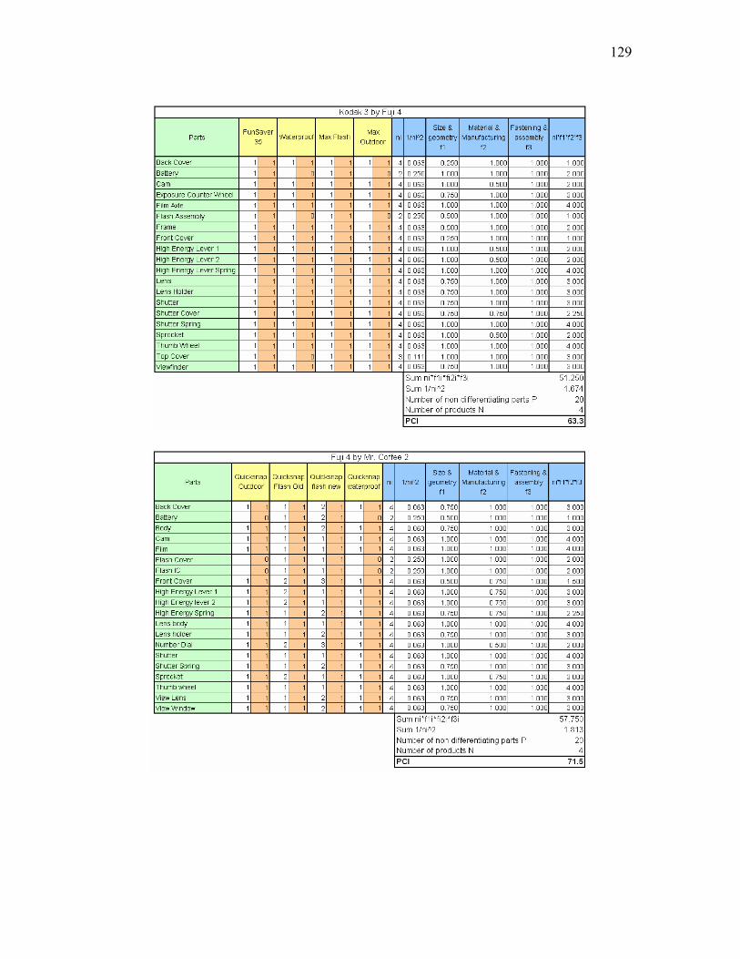
129

130

131

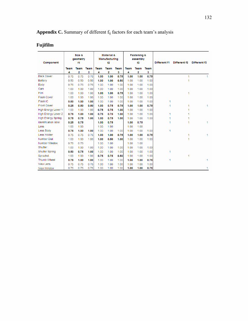
132

Appendix C. Summary of different fij factors for each team’s analysis

Fujifilm

133

Mr. Coffee

134

Appendix D. Computation of the PCI for the second experiment

135

136

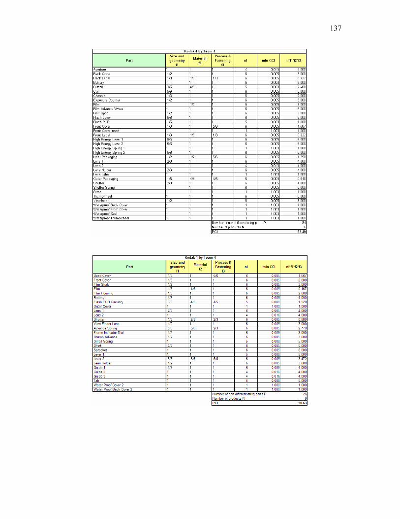
137

138

139

Appendix E. Computation of the CMC for the five product families analyzed

PaperPro

Logitech

140

Microsoft

Fujifilm

141

Kodak

142

VITA Henri Thevenot is a Graduate Research Assistant in the Harold and Inge Marcus Department of

Industrial and Manufacturing Engineering at The Pennsylvania State University working with Dr.

Timothy W. Simpson. He obtained two Master of Science degrees in Industrial and

Manufacturing Engineering in December 2003. The first one, also called Diplôme d’Ingénieur,

was obtained from the Ecole Centrale de Lyon (France), one of the top three French

multidisciplinary engineering schools (known as Grandes Ecoles d’Ingénieurs). The second one

was obtained from the Pennsylvania State University, ranked third in the United States. His

Master’s thesis, at the Pennsylvania State University, was titled, “A Comparison of Commonality

Indices for Product Family Design.”

Over the course of his studies at The Pennsylvania State University, Henri has been heavily

involved in research and teaching. He conducted his research in the Engineering Design and

Optimization Group (EDOG) Laboratory which is comprised of two faculty members and ten

students. He has written twenty three papers thus far in his last two years, and one book chapter.

Henri also helped teach two undergraduate level classes (in the Department of Engineering

Design and in the Department of Mechanical and Nuclear Engineering).