a meshless lbie/lrbf method for solving the nonlinear ... meshless lbie/lrbf method for solving the...

Copyright © 2015 Tech Science Press CMES, vol.105, no.2, pp.87-122, 2015

A Meshless LBIE/LRBF Method for Solving the NonlinearFisher Equation: Application to Bone Healing

K. N. Grivas1, M. G. Vavva1, E. J. Sellountos2, D. I. Fotiadis3

and D. Polyzos1,4

Abstract: A simple Local Boundary Integral Equation (LBIE) method for solv-ing the Fisher nonlinear transient diffusion equation in two dimensions (2D) is re-ported. The method utilizes, for its meshless implementation, randomly distributednodal points in the interior domain and nodal points corresponding to a Bound-ary Element Method (BEM) mesh, at the global boundary. The interpolation ofthe interior and boundary potentials is accomplished using a Local Radial BasisFunctions (LRBF) scheme. At the nodes of global boundary the potentials andtheir fluxes are treated as independent variables. On the local boundaries, potentialfluxes are avoided by using the Laplacian companion solution. Potential gradientsare accurately evaluated without RBFs via a LBIE, valid for gradient of poten-tials. Nonlinearity is treated using the Newton-Raphson scheme. The accuracy ofthe proposed methodology is demonstrated through representative numerical ex-amples. Fisher equation is solved here via the LBIE/LRBF method in order topredict cell proliferation during bone healing. Cell concentrations and their gradi-ents are numerically evaluated in a 2D model of fractured bone. The results aredemonstrated and discussed.

Keywords: Fisher equation, Local Boundary Integral Equation Method, LBIE,Local Radial Basis Functions, Bone healing.

1 Introduction

Linear and nonlinear transient diffusion is associated with problems dealing withheat conduction in materials, structures and tissues, mass transfer, surface anneal-ing, welding and drilling of metals, chloride diffusion in concrete, pattern formation

1 Department of Mechanical Engineering and Aeronautics, University of Patras, Patras, Greece.2 Instituto Seperior Tecnico CEMAT, Lisbon, Portugal.3 Department of Materials Science and Engineering, University of Ioannina.4 Corresponding author. E-mail: [email protected]; Tel: (0030) 2610969442

88 Copyright © 2015 Tech Science Press CMES, vol.105, no.2, pp.87-122, 2015

in population dynamics and solidification processes. In the context of biology andfor the difficult and complicated problem of cell proliferation and migration a math-ematical model that has been widely used for the simulation of those processes isthe nonlinear partial differential equation proposed by [Fisher (1937)]. Specifically,for the case of bone regeneration unforced and/or forced Fisher partial differentialequation has been employed in order to model the bone healing process and predictrelative experimental observations [Isaksson, Donkelaar, Huiskes and Ito (2008);Garcia-Aznar, Kuiper, Gomez-Benito, Doblare and Richardson (2007); Andreykiv,Van Keuler and Prendergast (2008); Gunzburger, Hou and Zhu (2005); Moreo,Gaffney, Garcia-Aznar and Doblare (2010); Sengers, Please, Oreffo (2007)].

Due to nonlinear form of Fisher’s equation, analytical solutions are very difficult tobe performed in two or three dimensions and when they exist are confined to specialcases and simple geometries [Petrovskii and Shigesada (2001)]. For this reason re-sort should be made to numerical methods, which are able to solve such problems.In the rich literature of the numerical methods that are able to treat nonlinear dif-fusion partial differential equations one can mention the Finite Element Method(FEM) [Garcia-Aznar, Kuiper, Gomez-Benito, Doblare and Richardson (2007)],the Finite Differences Method (FDM) [Khiari and Omrani (2011)], the Finite Vol-ume Method (FVM) [Prokharau, Vermolen and Garcia-Aznar (2013)], the DualReciprocity Boundary Element Method (DR-BEM) [Guo, Chen and Gao (2012)],the Domain-BEM [Mohammadi, Hematiyan and Marin (2010)] and the Analog-BEM [Katsikadelis and Nerantzaki (1999)]. The main problem with FEM, FDMand FVM is their requirement for domain discretization, which could be problem-atic or time consuming for complicated geometries, while the boundary methodssuch as DR-BEM and Analog-BEM are associated with very time consuming fullypopulated and non-symmetric matrices.

The last fifteen years, meshless methods have received considerable attention sincethey are able to treat efficiently nonlinear problems without meshing requirements.In the area of linear and nonlinear diffusion problems one has to mention theMeshless Local Petrov-Galerkin (MLPG) method [Lin and Atluri (2000); Sladek,Sladek, Tan and Atluri (2008); Chen and Liew (2011); Mirzaei and Dehgham(2011)] the Local Boundary Integral Equation (LBIE) method [Sladek, Sladek andZhang (2004)], [Shirzadi, Sladek, Sladek (2013); Popov and Bui (2010)], the Mesh-free Point Collocation Method (MPCM) [Bourantas and Burganos (2013); Sarlerand Vertnik (2006)], [Trobec, Kosec, Sterk and Sarler (2012)] and the Meshlesslocal radial point interpolation (MLRPI) method [Shivanian (2013)]. More detailson meshless methods one can find in the books of Atluri and Shen [Atluri and Shen(2002); Atluri (2004); Li and Liu (2007)] and in the very recent review work of[Sladek, Stanak, Han, Sladek, Atluri (2013); Atluri and Zhu (1998); Zhu, Zhang

A Meshless LBIE/LRBF Method for Solving the Nonlinear Fisher Equation 89

and Atluri (1998, 1999)] were the first who proposed the meshless MLPG andLBIE methods, respectively, as a simple and less-costly alternative to the FEM andBEM, respectively. Their methods are characterized as meshless methods becausethe interpolation is accomplished through randomly distributed points covering thedomain of interest and characterized by no-connectivity requirements. The fieldsat the local and global boundaries as well as in the interior of the subdomains areusually approximated by the Moving Least Squares (MLS) approximation scheme.The local nature of the sub-domains leads to a final linear system of equations thecoefficient matrix of which is sparse and not fully populated.

After the pioneering work of [Zhu, Zhang and Atluri (1998)], meshless LBIEmethod have received considerable attention due to its accuracy as integral equa-tion method and its flexibility to avoid any kind of mesh. Very recently [Sell-ountos, Sequeira and Polyzos (2009)] proposed a stable, accurate and very simplemeshless LBIE method for solving elastostatic problems, which utilizes an efficientLocal Radial Basis Functions (LRBF) interpolation scheme [Sellountos, Sequeiraand Polyzos (2010); Hardy (1990)] instead of MLS approximation and combinestechniques applying in both BEM and LBIE method. At the boundaries of localdomains tractions are eliminated with the aid of the companion solution of elasto-static equation [Li and Liu (2007)], while at the global boundary displacements andtractions are treated as independent variables. All the integrals at local and globalboundaries are evaluated as in the case of a BEM formulation and the displacementnodal values are interpolated through the LRBFs. In that way, the LBIE/LRBFmethod proposed by [Sellountos, Polyzos and Atluri (2012)] solves the elastostaticproblem very efficiently avoiding derivatives of LRBFs and concluding to a finalsystem of algebraic equations with banded coefficient matrix.

In the present work, that methodology is implemented for the case of two dimen-sional (2D) transient diffusion problems described by the nonlinear Fisher equation.Then the new LBIE/LRBF method is employed to provide numerical predictionsfor cell proliferation in a 2D model of fractured bone. As in [Sellountos, Sequeiraand Polyzos (2009)], at each internal or boundary point a circular support domainis centered and the LBIE valid for the potential field and its flux is assigned. BothLBIEs are derived with the aid of Laplace fundamental solution, thus containingvolume integrals coming from transient and nonlinear terms that act as internalsources. On the local circular boundaries, all the integrals that contain the fluxes ofthe potential field are eliminated via companion solutions derived for the needs ofthe present work. The circular local domains are sectored into subregions and theirboundary is discretized into line quadratic elements that in turn introduce a numberof “temporary” nodal points which, however, have not any relation with the ini-tially considered nodal points. Then, all the involved surface and volume integrals


are very accurately evaluated with the aid of the integration technique proposedby [Gao (2002, 2005)], while the potential fields defined at the “temporary” nodesare interpolated through the LRBF scheme illustrated in [Sellountos, Sequeira andPolyzos (2009)]. In that way, the final system of algebraic equations is derived veryefficiently without the use of derivatives of the LRBF interpolants. The treatmentof the nonlinearity is accomplished with the aid of the Newton-Raphson schemeand the problem is solved without the need of any derivative of the utilized LRBFs.It should be mentioned here that the idea of using “temporary” nodal points wasfirst proposed by [Popov and Bui (2010)] and that was unintended ignored in [Sell-ountos, Polyzos and Atluri (2012)]. However, the LBIE methodology of Popov andBui is completely different to the ones proposed in [Sellountos, Polyzos and Atluri(2012)] and here.

The paper is organized as follows: The LBIEs valid for potentials and their fluxesare explicitly derived in the next section. The LRBF interpolation scheme em-ployed in the present method is illustrated in section 3. The numerical implemen-tation of the proposed LBIE/LRBF methodology for solving the Fisher equation ispresented in section 4, while representative benchmark problems that demonstratethe accuracy of the method are provided in section 5. Finally, the LBIE/LRBFmethod is employed to solve the Fisher equation for a 2D model dealing with cellproliferation in a bone healing process. The obtained results are demonstrated anddiscussed in section 6.

2 LBIEs for Fisher’s non-linear transient diffusion equation

In this section the LBIEs used in the present method are illustrated. Consider a two-dimensional domain V surrounded by a surface S and a concentration or populationdensity function ϕ(x1,x2, t) at the spatial position (x1,x2) and time t. According toFisher equation, the field ϕ(x1,x2, t) satisfies the partial differential equation:

D1∂2i ϕ = ∂tϕ +D2ϕ (1−aϕ) (1)

where D1,D2,a are positive constants depending on the nature of the problem and∂i,∂t partial derivatives with respect to spatial coordinate xi, i = 1,2 and time, re-spectively.

The boundary conditions are assumed to be

ϕ (x) = ϕ0 (x) , x(x1,x2) ∈ Sϕ

q(x) =∂ϕ (x)

∂n= q0 (x) , x(x1,x2) ∈ Sq

(2)

with n denoting the unit vector normal to the global boundary, ϕ0,q0 prescribedfunctions and Sϕ ∪Sq ≡ S.


Making use of the finite-differences scheme

∂tϕp+1 =

ϕ p+1−ϕ p

∆t+O(∆t) (3)

and ignoring higher order terms, the governing equation (1) obtains the form

∂2i ϕ

p+1 =

[1

D1∆t+

D2

D1

]ϕ

p+1− 1D1∆t

ϕp− aD2

D1

(ϕ

p+1)2(4)

Utilizing the fundamental solution of Laplace equation and applying Green’s inte-gral identity one obtains the following integral equation

αϕp+1 (x)+

∫Γ

q∗ (x,y)ϕp+1 (y)dSy

=∫Γ

ϕ∗ (x,y)qp+1 (y)dSy

+∫V

ϕ∗ (x,y)

[− 1

D1∆t− D2

D1

]ϕ

p+1 (y)+1

D1∆tϕ

p (y)

dVy

+∫V

aD2

D1ϕ∗ (x,y)

(ϕ

p+1 (y))2

dVy

(5)

where the coefficient α takes the value 0.5 when x∈ S and S being a smooth bound-ary and the value 1 when x ∈V , while the kernels ϕ∗,q∗ have the form

ϕ∗ =− 1

2πlnr

q∗ =− 12πr

(ny, r)

r = |y−x| , r =y−x|y−x|

(6)

A group of N randomly distributed points x(k),k = 1, ..,N that cover the domain ofinterest V are considered, while the global boundary Sϕ ∪Sq ≡ S is defined througha BEM mesh with Z totally nodal points. At any point x(k) a circular domain Ω(k)

(with boundary ∂Ω(k)) is centered, called support domain of x(k) and illustrated inFigure 1.

Employing Green’s second identity for the domain being between the boundaries Sand ∂Ω(k), the integral representation (5) obtains the form:


Figure 1: Local domains and local boundaries used for the LBIE representation ofdensity function ϕ(x(k)).

αϕp+1(

x(k))+

∫Γ(k)∪∂Ω(k)

q∗(

x(k),y)

ϕp+1 (y)dSy

=∫

Γ(k)∪∂Ω(k)

ϕ∗(

x(k),y)

qp+1 (y)dSy

+∫

Ω(k)

ϕ∗(

x(k),y)[− 1

D1∆t− D2

D1

]ϕ

p+1 (y)+1

D1∆tϕ

p (y)

dVy

+∫

Ω(k)

aD2

D1ϕ∗(

x(k),y)[

ϕp+1 (y)

]2dVy

(7)

with Γ(k) being the part of the global boundary intersected by the circular supportdomain of point x(k) (Fig. 1).

The coefficient α is equal to 1 for internal points and 1/2 for points lying on theglobal boundary Γ with smooth tangent. As it has been already mentioned, in thepresent formulation, boundary points are imposed with the aid of a BEM mesh.Thus, in case of a non-smooth boundary partially discontinuous elements at bothsides of a corner are considered. Consequently, the coefficient α is always equal to


0.5 for all the boundary points x(k).In order to get rid of fluxes at the local boundary ∂Ω(k) the companion solution ofLaplace equation can be utilized [Atluri (2004)] and Eq. (7) becomes

αϕp+1(

x(k))+

∫Γ(k)∪∂Ω(k)

q∗(

x(k),y)

ϕp+1 (y)dSy

=∫

Γ(k)

[ϕ∗(

x(k),y)−ϕ

c(

x(k),y)]

qp+1 (y)dSy

+∫

Ω(k)

[ϕ∗(

x(k),y)−ϕ

c(

x(k),y)][

− 1D1∆t

− D2

D1

]ϕ

p+1 (y)+1

D1∆tϕ

p (y)

dVy

+∫

Ω(k)

aD2

D1

[ϕ∗(

x(k),y)−ϕ

c(

x(k),y)][

ϕp+1 (y)

]2dVy

(8)

where ϕc represents the companion solution ϕc = − 12π

lnrk with rk denoting theradius of the support domain of point x(k).An integral representation for the gradient of ϕ p+1 can be obtained by applying thegradient operator on Eq. (7), i.e.

α∂iϕp+1(

x(k))+

∫Γ(k)∪∂Ω(k)

Q∗(

x(k),y)

ϕp+1 (y)dSy

=∫

Γ(k)∪∂Ω(k)

Φ∗ι

(x(k),y

)qp+1 (y)dSy

+∫

Ω(k)

Φ∗ι

(x(k),y

)[− 1

D1∆t− D2

D1

]ϕ

p+1 (y)+1

D1∆tϕ

p (y)

dVy

+∫

Ω(k)

aD2

D1Φ∗ι

(x(k),y

)[ϕ

p+1 (y)]2

dVy

(9)

where the vectors Φ∗i ,Q∗i correspond to ∂iϕ

∗,∂iq∗, respectively.

The integral defined at the local boundary ∂Ω(k) and containing the fluxes qp+1 canbe eliminated with the aid of a new companion solution derived in Appendix A.


Thus, following the procedure described in Appendix A Eq. (9) can be written as

α∂iϕp+1(

x(k))+

∫Γ(k)∪∂Ω(k)

[Q∗i(

x(k),y)−Qi

(x(k),y

)]ϕ p+1 (y)dSy

=∫

Γ(k)

[Φ∗i

(x(k),y

)−Φ

ci

(x(k),y

)]qp+1 (y)dSy

+∫

Ω(k)

[Φ∗i

(x(k),y

)−Φ

ci

(x(k),y

)]

[− 1

D1∆t− D2

D1

]ϕ

p+1 (y)+1

D1∆tϕ

p (y)

dVy

+∫

Ω(k)

Gci

(x(k),y

)ϕ

p+1 (y)dSy

+∫

Ω(k)

aD2

D1[Φ∗i

(x(k),y

)−Φ

ci

(x(k),y

)][ϕ

p+1 (y)]2

dVy

(10)

where

Φ∗i =−

12πr

∂ir

Φci =−

12π

r2

r2k

∂ir

Q∗i =1

2πr2 [2(nm∂mr)∂ir−ni]

Qci =−

12π

rr3

k[(nm∂mr)∂ir+ni]

Gci =−

32π

1r3

k∂ir

(11)

The integral equations (8) and (10) represent the LBIEs for the (p+1) - step fieldsϕ p+1 and ∂iϕ

p+1, respectively at any interior and boundary point of the analyzeddomain.

3 The LRBF interpolation scheme

In the present section the LRBF interpolation scheme employed in the present workis illustrated. Consider a domain V surrounded by a boundary Γ covered by arbi-trarily distributed nodal points

x(k),k = 1,2, ..,N (12)


as shown in Fig. 1. Each nodal point x(k) is considered as the centre of a smallcircular domain Ωk of radius rk called support domain of x(k). All support domainsof a group of adjacent nodal points that satisfy the condition∣∣∣x(k)−x( j)

∣∣∣< rk + r j (13)

form a domain called domain of influence of point x(k) (Fig. 2). The supportdomains of all the considered internal and boundary points are overlapping circlesthat cover completely the domain of interest. The support domains of the nodalpoints that contain a point x form the domain of definition of point x, also illustratedin Fig. 2

Figure 2: Domain of influence of the point x( j) and domain of definition of point x.

At any point x of Ω, the interpolation of the unknown field ϕ(x), is accomplishedby the relation

ϕ (x) = BT (x) ·a(x)+PT (x) ·b(x) (14)

or

ϕ (x) =[

BT (x) PT (x)]·[

a(x)b(x)

](15)


where

x =[

x1 x2]T

a =[

a1 a2 · · · an]T

b =[

b1 b2 · · · bm]T

B(x) =[

W(x,x(1)

)W(x,x(2)

)· · · W

(x,x(n)

) ]TP(x) =

[P1 (x) P2 (x) · · · Pm (x)

](16)

with n representing the total number of nodal points belonging to the domain ofdefinition of point x and m the number of complete polynomials with m < n. Thevectors a and b stand for unknown coefficient vectors that depend on the locationof the nodal points belonging to the domain of definition of point x. P(x) is a vectorcontaining the monomial basis, i.e.

PT (x) =[

1 x1 x2]

for m = 3

PT (x) =[

1 x1 x2 x21 x1x2 x2

2]

for m = 6(17)

and W(x,x(n)

)are RBFs defined in the present work as multiquadric LRBFs (MQ-

LRBFs)

W(

x,x(n))=

√(x1− x(n)2

)2+(

x2− x(n)2

)2+C2 (18)

For the domain of definition of x, C is a constant the value of which is taken equalto [Hardy (1990)]

C (x) = 0.8151n

n

∑i=1

di (19)

with di being the distance between every nodal point of the domain of definition ofx and its closest nodal neighbor.

The definition of the unknown vectors a and b is accomplished by imposing aninterpolation passing of Eq. (15) through all nodal points x(n), i.e.

ϕ

(x(e))=[

BT(x(e))

PT(x(e)) ]·[

ab

], e = 1,2, . . . ,n (20)

and considering the extra system of algebraic equations

n

∑e=1

Pl

(x(e))

ae = 0, l = 1,2, . . . ,m (21)


Thus, the following system of equations is formed:[B0 P0PT

0 0

][ab

]=

[f(e)0

](22)

where

B0 =

W(x(1),x(1)

)W(x(1),x(2)

)· · · W

(x(1),x(n)

)W(x(2),x(1)

)W(x(2),x(2)

)· · · W

(x(2),x(n)

)· · · · · · · · · · · ·

W(x(n),x(1)

)W(x(n),x(2)

)· · · W

(x(n),x(n)

) (23)

P0 =

P1(x(1))

P2(x(1))· · · Pm

(x(1))

P1(x(2))

P2(x(2))· · · Pm

(x(2))

· · · · · · · · · · · ·P1(x(n))

P2(x(n))· · · Pm

(x(n)) (24)

and

f(e) =[

ϕ(1) ϕ(2) · · · ϕ(n)]T

(25)

In view of Eq. (22) the coefficient vector[

a b]T is equal to[

ab

]= A−1

[f(e)0

](26)

where A is the symmetric matrix

A =

[B0 P0PT

0 0

](27)

Finally, the interpolation Eq. (15) obtains the form

ϕ (x) =[

BT (x) PT (x)]·A−1 ·

[f(e)0

]= R

(x,x(e)

)· f(e) (28)

where

R(

x,x(e))=[

R(1) R(2) · · · R(n)]

R(e) =n

∑i=1

Bi (x)A−1ie +

m

∑j=1

Pj (x)A−1(n+ j)e,e = 1,2, . . . ,n

(29)

with A−1qr representing the (qr)-element of the matrix A−1.


The LRBF shape functions (29) depend uniquely on the distribution of scatterednodes belonging to the support domain of the point where the field is interpolated.The positive definitiveness of the just described LRBFs is accomplished with theuse of the additional polynomial term in Eq. (14) and the homogeneous constraintcondition (21). More details on the LRBFs one can find in the book of [Buh-mann (2004)] and in the representative works of [Sellountos and Sequeira (2008a,2008b); Wang and Liu (2002); Gilhooley, Xiao, Batra, McCarthy and Gillespie(2008)] and [Bourantas, Skouras, Loukopoulos, Nikiforidis (2010)].

4 Numerical implementation of the proposed LBIE/LRBF method

In this section the numerical implementation of the proposed LBIE/LRBF method-ology is reported.

As it has been explained in section 2, the function ϕ p+1(x(k)) defined at any internalpoint x(k) with support domain that does not intersect the global boundary, admitsa LBIE of the form

ϕp+1(x(k))+

∫∂Ω(k)

q∗(x(k),y)ϕ p+1(y)dSy

=∫

Ω(k)

[ϕ∗(x(k),y)−ϕ

c(x(k),y)][− 1

D1∆t− D2

D1

]φ

p+1(y)+1

D1∆tφ

p(y)

dVy

+∫

Ω(k)

aD2

D1

[ϕ∗(x(k),y)−ϕ

c(x(k),y)][

ϕp+1(y)

]2dVy

(30)

Since Ω(k) represents a circular domain, the above LBIE can be written in polarcoordinated as [Gao (2002, 2005)].

ϕp+1(x(k))+

∫∂Ω(k)

q∗(x(k),y)ϕ p+1(y)dSy

=∫

∂Ω(k)

F(1)(x(k),y)R(x(k),y)

dSy +∫

∂Ω(k)

F(2)(x(k),y)R(x(k),y)

dSy

(31)

where

F(1)(x(k),y)

=

R(x(k),y)∫0

[ϕ∗(x(k),x)−ϕ

c(x(k),x)]·[− 1

D1∆t− D2

D1

]ϕ

p+1(x)+1

D1∆tϕ

p(x)

rdr

(32)


F(2)(x(k),y) =R(x(k),y)∫

0

aD2

D1

[ϕ∗(x(k),x)−ϕ

c(x(k),x)][

ϕp+1(x)

]2rdr (33)

dSy = R(

x(k),y)

dϕ

x = x(k)+ rr

r =x(k)−y∣∣x(k)−y

∣∣R(

x(k),y)=∣∣∣x(k)−y

∣∣∣(34)

Considering, just for demonstration purposes, 4 quadratic line elements across thecircumferential direction and one quadratic element in radial direction, the LBIE(31) obtains the form

ϕp+1(x(k))+

4

∑b=1

3

∑n=1

1∫−1

q∗N(bn)Jbdξ

ϕp+1(x(3bn))

−

4

∑b=1

3

∑n=1

1∫−1

3

∑m=1

1∫−1

[ϕ∗−ϕc]

[− 1

D1∆t− D2

D1

]rN(m)Jmdξ

N(bn)Jbdξ

ϕp+1(x(mbn))

−

4

∑b=1

3

∑n=1

1∫−1

3

∑m=1

1∫−1

[ϕ∗−ϕc]

1D1∆t

rN(m)Jmdξ

N(bn)Jbdξ

ϕp(x(mbn))

−

4

∑b=1

3

∑n=1

1∫−1

3

∑m=1

1∫−1

[ϕ∗−ϕc]

aD2

D1rN(m)Jmdξ

N(bn)Jbdξ

[ϕ p(x(mbn))]2

= 0

(35)

where N(bn), N(m) are the shape functions corresponding to quadratic line elementsin the circumferential and radial direction, respectively, Jb and Jm are the corre-sponding Jacobians of the transformation from the global to the local coordinatesystems ξ and the vector x(mbn) represents all the radial and circumferential nodesindicated with open circles in Fig. 3.

It should be noticed here that those points x(mbn) have not any relation with theinitially considered nodal points, which in Fig. 3 are indicated with the full circles.Thus, in Fig. 3 the full circles represent the nodal points used for the meshlessprocedure while the open circles represent the “temporary” nodal points, which arethe same for any non-intersected support domain. Considering the 16 “temporary”


(a)

(b)

Figure 3: (a) The support domain of an internal point x(k) sectored and discetizedby line quadratic elements in the circumferential and radial direction. The fullcircles stand for the nodal points used for the meshless treatment of the structure,while the open circles represent the “temporary” nodal points. (b) The field at each“temporary” nodal point is interpolated via LRBFs defined via the nodal points (redpoints) belonging in the support domain (red circle) of the “temporary” nodal pointindicated by the arrow.


nodal points of Fig. 3(a), Eq. (33) obtains the form

16

∑l=1

ϕ(l)

ϕp+1(x(l))+

16

∑l=1

Ψ(l)

ϕp(x(l))+

16

∑l=1

Z(l)[ϕ

p+1(x(l))]2

= 0 (36)

where ϕ(l), Ψ(l), Z(l) represent all the integrals involved in (35) and evaluated oncesince they are the same for all non-intersected support.

For a boundary point x(k), the corresponding LBIE is given by equation (8) with a=12 . Considering the discretization shown in Fig. 3(b), adopting polar coordinatesand following the procedure described previously, equation (8) is finally written as

9

∑l=1

Q(l)ϕ

p+1(x(l))+5

∑c=1

Q(c)q qp+1(x(c))+

9

∑l=1

X (l)ϕ

p(x(l))+9

∑l=1

Ω(l)[ϕ

p+1(x(l))]2+b=0

(37)

where x(c) represents the five nodal points that define the portion of the globalboundary and b is scalar coming from the application of boundary conditions.

As in (36), all the integrals defined across the circumferential direction are alreadyknown. The only integrals that have to be evaluated here are those defined acrossthe global boundary.

The key idea of the present LBIE/LRBF method is that Eq. (36) is the same forall internal points with complete support domains and all the aforementioned “tem-porary” nodal fields are interpolated via the LRBF scheme illustrated in previoussection. Consequently, Eqs. (36) and (37) obtain the form, respectively

16

∑l=1

ϕ(l)

∑i

R(x(l),x(i))ϕ p+1(x(l))+16

∑l=1

Ψ(l)

∑i

R(x(l),x(i))ϕ p(x(l))

+16

∑l=1

Z(l)∑

iR(x(l),x(i))

[ϕ

p+1(x(l))]2

= 0

(38)

16

∑l=1

Q(l)ϕ ∑

iR(x(l),x(i))ϕ p+1(x(l))+

5

∑c=1

Q(c)ϕ qp+1(x(l))+

9

∑l=1

X (l)∑

iR(x(l),x(i))ϕ p(x(l))

+9

∑l=1

X (l)∑

iR(x(l),x(i))

[ϕ

p+1(x(l))]2

+b = 0

(39)

where x(i) represents all the nodal points belonging in the support domain of eachnodal or “temporary” point, shown in Fig. 4 by red full circles.


Both Eqs. (38) and (39) can be written in vector form as

H(1) · fp+1 +H(2) ·vp+1 = H(3) · fp (40)

(a)

(b)

Figure 4: (a) The support domain of a boundary point x(k) intersected by the globalboundary of the structure and discretized as in Figure 3. The full circles stand forthe nodal points used for the meshless treatment of the structure, while the opencircles represent the “temporary” nodal points. (b) The field at each “temporary”nodal point is interpolated via LRBFs defined via the nodal points (red points) be-longing in the support domain (red circle) of the “temporary” nodal point indicatedby the arrow.


P(1) · fp+1 +G(1) ·qp+1 +P(2) ·vp+1 = P(3) · fp +b (41)

where fp+1, qp+1, vp+1 are vectors comprising all the unknown values of ϕ p+1,qp+1,

(ϕ p+1

)2, respectively, while the vector fp contains all the nodal values of ϕ p

known from the previous time step.

Collocating Eqs. (40) and (41) at all internal and boundary nodal points one obtainsthe following non-linear system of algebraic equations

f (x) = A ·x−B = 0 (42)

where the vector x contains the unknown nodal values ϕ p+1,qp+1 and (ϕ p+1)2 andthe vector B is known from the previous time step and the boundary conditions.

The non-linear system (42) is solved according to standard Newton-Raphson algo-rithm adopting the following steps:

1. Make an initial guess for the unknown vector x, let x(0). In the present workthe initial guess was x(0)= 0.

2. Evaluate the Jacobian matrix ∇x f (x). Since the only non-linear term is thatcorresponding to the nodal values (ϕ p+1)2, it is apparent that the Jacobian isa linear matrix with respect to x.

3. Solve the linear system ∇x(0) f (x(0)) ·(x(1)−x(0)

)= − f (x(0)) and find the

new vector x(1).

Supposing that convergence is accomplished in the (k+1)-step, then the final vectorx(k+1) satisfies the linear system ∇x(k) f (x(k)) ·

(x(k+1)−x(k)

)=− f (x(k)).

As soon as the functions ϕ p+1 and qp+1 are known, the vector ∂iϕp+1 can be eval-

uated either by taking directly the gradient of the LRBF-interpolated ϕ p+1 or byconsidering the LBIE given by Eq. (10).

5 Benchmark problems

In the present section, the LBIE/BEM method illustrated in previous sections istested with two linear benchmark problems and one nonlinear problem with a so-lution taken by the FEM.

Consider the 1m×1m rectangular plate shown in Fig. 5(a). The upper side ofthe plate is subjected to a sudden thermal loading of unit temperature T=1.0 andremains at that temperature for the rest of time. The other three sides of the plateare isolated with zero temperature fluxes and all the material properties are assumed


to be equal to unity. The just described transient thermal diffusion boundary valueproblem is represented by the following equations:

∂2i T (x1,x2, t) = ∂tT (x1,x2, t)

T (x1, l, t) = l,

∂T (x1,x2, t)∂x1

∣∣∣∣x1=0

=∂T (x1,x2, t)

∂x1

∣∣∣∣x1=1

=∂T (x1,x2, t)

∂x1

∣∣∣∣x2=0

(43)

The analytical solution of (43) has the form [Carter, Beaupre, Giori and Helms(1998)]:

T (x1,x2, t) = 1− 4π

∞

∑n=0

(−1)n

n+1e−

(2n+1)2π2t4 cos

(2n+1)πx2

2(44)

For the LBIE/LRBF solution of the problem 81 uniformly distributed internal pointshave been considered, while the external boundary has been discretized with 16quadratic line elements. The support domains have been selected to be the samefor all nodes and equal to 0.566 m. The temperature at (x, y) = (0.5, 0.5) has beencalculated and compared to analytical ones provided by Eq. (44). As it is apparentin Fig. 5(b) the agreement is excellent.

The previous problem has also been solved utilizing 185 non-uniformly distributednodal points (Fig. 6a) with support domain of radius equal to 0.3456m. The tem-perature at (x, y) = (0.5, 0.5) as a function of time has been evaluated and comparedto the corresponding solution concerning uniformly distributed points in Fig. 6b.The comparison shows an excellent agreement.

The accuracy of the present method in calculating the gradient of the field at anypoint of the analyzed domain is also tested. Concerning the above diffusion prob-lem of the rectangular plate the analytical solution for the temperature gradient isgiven by

∇T =4π

∞

∑n=0

(−1)n

n+1e−

(2n+1)2π2t4

(2n+1)π

2sin

(2n+1)πx2

2x2 (45)

with x2 representing the unit vector at x2 direction.

The gradient of the temperature at the (x, y) = (0.5, 0.5) has been evaluated with theaid of the LBIE of Eq. (10) and it is compared with the analytical one provided byEq. (45). As it is shown in Fig. 7 the agreement between numerical and analyticalresults is excellent.

As it has been already mentioned in section 4, the gradient of the density functionϕ p+1 can be evaluated either by using the LBIE of Eq. (10) or via the derivatives of


(a)

(b)

Figure 5: (a) Internal and boundary nodal points considered for the LBIE/LRBFsolution of the problem described by Eq. (43). (b) Time history of temperature at(x, y) = (0.5, 0.5).


(a)

(b)

Figure 6: The problem of Fig. 5 with non-unform distribution of nodal points.(a) Internal and boundary nodal points considered for the LBIE/LRBF solution ofproblem described by Eq. (43). (b) Time history of temperature at (x, y) = (0.5,0.5).


Figure 7: Time history of the gradient of temperature and comparison with theanalytical solution (45).

the local radial basis interpolation functions. Comparing the accuracy provided bythe two methodologies, the general conclusion is that Eq. (10) is always superiorto derivatives of LRBFs especially at points lying near and on the global boundaryof the considered domain. For internal points far from the external boundary theprovided accuracy is comparable. For example, the numerical error appearing in theevaluation of ∂iϕ via the LBIE of Eq. (10) at points A(1.0, 1.0), B(0.5, 0.5), C(0.1,0.1) (Fig. 5(a)) is 0.08%, 0.1% and 0.07% respectively, while via the derivativesof LRBFs at the corresponding points ∂iϕ is 2.1%, 1.0% and 1.8%. Knowingthat the interpolation provided by the LRBFs near to the boundary points is betterthan that provided by their derivatives, the aforementioned behaviour is expectablesince the evaluation of ∂iϕ through Eq (10) is accomplished by avoiding the useof derivatives of LRBFs. In that sense, the evaluation of ∂iϕ through the LBIE ofEq. (10) could not be characterized as “expensive” because for points lying nearto the boundary provides better accuracy, while for internal points all the involvedintegrals in Eq. (10) are evaluated once as in the case of Eq. (9) explained in section4.

The nonlinear version of the above mentioned problem has been solved with thecoefficients D1, D2 and α of Eq. (1) being D1 = D2 = α=1. The obtained so-lution is compared to the corresponding one taken through the commercial FEMpackage COMSOL Multiphysics 4.0a and depicted in Fig. 8. As it is apparent, the


agreement is very good.

Figure 8: Temperature at (x, y) = (0.5, 0.5) as a function of time for the nonlinearversion of problem (43). Comparison between the results taken from COMSOLMultiphysics 4.0a and the present LBIE/LRBF.

In the sequel, the accuracy of the present LBIE/LRBF method in solving the afore-mentioned nonlinear problem with the non-uniformly point distribution of Fig. 6is checked. As it is shown in Fig. 9 the agreement between the numerical resultstaken through LBIE and those taken through the commercial FEM package COM-SOL Multiphysics 4.0a is excellent.

Finally, the convergence while making the mesh denser for the two cases (linearand non-linear Fisher equation) is examined. Both uniformly and non-uniformlydistributed nodal points have been considered. Three mesh cases correspondingto 49, 81 and 121 nodal points have been considered. Comparing to analyticaland FEM solutions, the convergence error for a nodal point in the center of therectangular plate (x, y) = (0.5, 0.5) and in the upper left corner near the boundary(x, y) = (0.9, 0.9), is calculated and reported in Tables 1 and 2.


Figure 9: Temperature at (x, y) = (0.5, 0.5) as a function of time for the nonlin-ear version of problem (43). Comparison on the obtained results when uniformlydistributed points and non- uniformly distributed points are considered.

Table 1: Mesh convergence error for the linear case (uniformly and non-uniformlydistributed nodes. Center and upper left node checked).

Linear CaseUniformly distributed nodes Non-uniformly distributed nodes

Nodes Center Node Upper-left Node Center Node Upper-left Node49 0.88% 0.90% 0.88% 0.90%81 0.82% 0.87% 0.82% 0.87%121 0.70% 0.75% 0.70% 0.75%

Table 2: Mesh convergence error for the non-linear case (uniformly and non-uniformly distributed nodes. Center and upper left node checked).

Non-linear CaseUniformly distributed nodes Non-uniformly distributed nodes

Nodes Center Node Upper-left Node Center Node Upper-left Node49 0.89% 0.94% 0.89% 0.94%81 0.84% 0.88% 0.84% 0.88%121 0.72% 0.79% 0.72% 0.79%


6 Application to bone healing

The process of bone fracture healing includes complex sequence of cellular eventswhich gradually restore the functional and mechanical bone properties, such asload-bearing capacity, stiffness and strength. Initially an inflammatory reactiontakes place and a hematoma is formed at the fracture gap forming an initial frac-ture callus that mainly consists of mesenchymal cells. Then along the bone mes-enchymal cells differentiate into osteoblasts which begin to synthesize bone. In theinterior of the initial callus and adjacent to the fracture mesenchymal cells differ-entiate into chondrocytes which synthesize cartilage. Subsequently blood vesselsare formed in the calcified cartilage which is then absorbed by osteoclasts. Thecartilage is replaced with ossified tissue and woven bone is formed via endochon-dral ossification of the callus. Finally the remodelling stage takes place in whichthe external callus is completely resorbed and in the fracture gap the disorganizedosteoclasts and osteoblasts are remodeled into cortical.

The determination of the underlying cellular mechanisms of bone healing remainsan open issue in the literature, despite the intensive work that has been conducted inthe field. To this end several mechanobiological computational models have beenproposed aiming to investigate and derive quantitative criteria that describe howmechanical stimulation affects tissue differentiation, growth, adaptation and main-tenance during bone healing [Gao (2002, 2005); Carter, Beaupre, Giori and Helms(1998); Claes and Heigele (1998); Prendergast (1997); Lacroix and Prendergast(2002)].

Most of the existing mechanobiology models incorporate bioregulatory modelswhich simulate the cellular processes such as dispersion and proliferation in bio-logic tissues via diffusion equations [Andreykiv, Van Keuler and Prendergast (2008);Claes and Heigele (1998); Prendergast (1997)]. [Lacroix and Prendergast (2002)]were the first to account for cell phenomena such as cell migration, proliferationand differentiation with the aid of diffusion equations. In this model progenitorcells were assumed to originate from different parts of healing bone i.e., perios-teum and bone marrow. [Bailon-Plaza and van der Meulen (2001)] also modeledmigration and proliferation of mesenchymal cells as well as chondrocyte and os-teoblast proliferation and differentiation via diffusive processes. In another study[Isaksson, Donkelaar, Huiskes and Ito (2008)] the cellular processes are directlyconnected with mechanical stimulation and act at cell-phenotype rates.

In all of the aforementioned studies numerical predictions of tissue differentiationand bone healing are derived using the Finite Element Method. Although FEMis a well-known and robust numerical method, when applied to problems dealingwith phase changes, suffers from global remeshing when new born surfaces or


material phases appear. On the other hand in meshless methods no backgroundcells are required for the numerical evaluation of the involved integrals [Sellountosand Sequeira (2008b); Wang and Liu (2002)]. This renders the present LBIE/LRBFmethod ideal for solving problems with moving or new-born boundaries since itavoids remeshing as new bone solidification regions appear.

In this subsection the LBIE/LRBF method is used for the first time for derivingpredictions of cell distribution in fractured bone during the healing process.

Although in most cases the description of cell activities is achieved by complicatedsystems of partial differential equations that correlate all the types of cells involvedin bone healing process, we adopt herein a simplified but rather effective model inwhich the concentration of all cell types is modeled as one parameter following theFisher Eq. (1) .

6.1 Geometrical model of healing bone

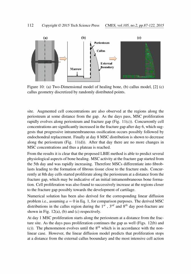
We considered a 2D model of callus based on previous mechanical models of heal-ing bone [Isaksson, Donkelaar, Huiskes and Ito (2008)] as shown in Fig. 10. Thecortical bone had inner and outer diameters of 14 mm and 20 mm [Isaksson, Donke-laar, Huiskes and Ito (2008); Claes and Heigele (1998)].

Cells were assumed to distribute according to Eq. (1) in which the field c(x1,x2, t)is the cell concentration within the callus region. Solution was derived for a = 1i.e., a non-linear diffusion equation. Cell parameters were considered equal tothose of mesenchymal stem cells (MSC) [Isaksson, Donkelaar, Huiskes and Ito(2008)].The diffusivity was equal to 0.65mm2/day [Isaksson, Donkelaar, Huiskesand Ito (2008)]. Initially fixed MSC concentrations were assumed at the perios-teum, the marrow interface and the interface between bone and callus at the fracturesite as depicted in Fig. 10. In addition, across the remainder external boundarieszero flux was assumed (Fig. 10(b)) i.e.,

dcdn

= 0 (46)

Numerical calculations were performed for 100 iterations which correspond to 40days post-fracture. The interior of the callus is fulfilled with 642 distributed nodes(Fig. 10c) with support domains of radius 0.4256.

6.2 Numerical Predictions of cell distribution during bone healing

The MSC distribution in the callus area during the process of bone healing is shownin Fig 11. The red colors correspond to maximum cell concentrations whereas blueones to minimum. As shown in Figs. 11(a), (b) MSCs initially (i.e., at the begin-ning and day 1) proliferate along the periosteum covering first the remote fracture


Figure 10: (a) Two-Dimensional model of healing bone, (b) callus model, [2] (c)callus geometry discretized by randomly distributed points.

site. Augmented cell concentrations are also observed at the regions along theperiosteum at some distance from the gap. As the days pass, MSC proliferationrapidly evolves along periosteum and fracture gap (Fig. 11(c)). Concurrently cellconcentrations are significantly increased in the fracture gap after day 6, which sug-gests that progressive intramembraneous ossification occurs possibly followed byendochondral replacement. Finally at day 8 MSC distribution is shown to decreasealong the periosteum (Fig. 11(d)). After that day there are no more changes inMSC concentrations and thus a plateau is reached.

From the results it is clear that the proposed LBIE method is able to predict severalphysiological aspects of bone healing. MSC activity at the fracture gap started fromthe 5th day and was rapidly increasing. Therefore MSCs differentiate into fibrob-lasts leading to the formation of fibrous tissue close to the fracture ends. Concur-rently at 8th day cells started proliferate along the periosteum at a distance from thefracture gap, which may be indicative of an initial intramembraneous bone forma-tion. Cell proliferation was also found to successively increase at the regions closerto the fracture gap possibly towards the development of cartilage.

Numerical solution has been also derived for the corresponding linear diffusionproblem i.e., assuming a = 0 in Eq. 1, for comparison purposes. The derived MSCdistributions in the callus region during the 1st , 3rd and 8th day post-fracture areshown in Fig. 12(a), (b) and (c) respectively.

At day 1 MSC proliferation starts along the periosteum at a distance from the frac-ture site. As the days pass proliferation continues the gap as well (Figs. 12(b) and(c)). The phenomenon evolves until the 8th which is in accordance with the non-linear case. However, the linear diffusion model predicts that proliferation stopsat a distance from the external callus booundary and the most intensive cell action


Figure 11: Predicted distributions of MSC in the callus during normal fracturehealing at (a) day 0 (beginning of the phenomenon), (b) day 1, (c) day 2, (d) day 5and (e) day 8.

Figure 12: MSC distributions in the callus during normal fracture healing at (a) day1, (b) day 3 and (c) day 8 derived from the linear diffusion equation.


is observed along the periosteun at a remote fracture site. On the other hand, inthe non-linear model the most increased cell activity is observed within the wholecallus region, which suggests that non-linear diffusion models can provide morerealistic decription of biological healing processes such as MSC proliferation.

Our findings make clear that meshless LBIE method seems promising in describ-ing complicated biological mechanisms that occur during bone healing. Thereforeenhanced bioregulatory models based on such computational methods could beproved effective for the quantitative evaluation of bone pahtologies.

7 Discussion - Conclusion

In this work a simple meshless LBIE/LRBF methodology for solving the 2D Fishernon-linear transient diffusion equation has been reported. The method utilizes acloud of randomly distributed and without any connectivity requirements pointscovering the domain of interest and a BEM mesh for the representation of the ex-ternal boundary. At each point a circular support domain is centered and a LBIEis assigned. The Laplace fundamental solution is employed and thus, each LBIEcontains surface integrals defined at the circular boundary of the support domainand volume integrals coming from the non-Laplacian terms of Fisher equation. Forintersected support domains by the global boundary, the corresponding LBIE com-prizes both integrals defined at the circular boundary of the support domain andintegrals defined at the portion of the global boundary intersected by the supportdomain of the considered point. A finite difference scheme is utilized for the timederivative of Fisher equation. In all the considered LBIEs, fluxes defined at thecircular boundaries are eliminated with the aid of companion solutions derived inthe framework of the present work. The accuracy of the addressed LBIE/LRBFmethod remains high as that provided by previous LBIE formulations proposed bySellountos, Polyzos and collaborators. As far as the efficiency of the method is con-cerned, the obvious improvement is the much faster formation of the final algebraicequations for all the internal points the support domain of which do not intersectthe global boundary. Because of that, the efficiency of the proposed LBIE/LRBFmethod is obviously better than that of our previous LBIE formulations and the for-mation of the algebraic equations of each internal point is at least ten times faster inthe present LBIE/LRBF formulation. That advantage becomes more pronouncedwhen uniform distributions of points are considered.

The novelty of the present meshless LBIE/LRBF formulation for solving nonlineartransient diffusion problems can be summarized as follows: (i) Utilizing the ideaproposed by [Popov and Bui (2010)] and [Sellountos, Polyzos and Atluri (2012)]and illustrated in section 4, all the points with non-intersected support domains havethe same LBIE given by Eq. (36). Thus, all the involved integrals are evaluated


once and the final system of algebraic equations is formed quickly and economi-cally. Making use of companion solutions derived in the present work, the proposedformulation is different than that of [Popov and Bui (2010)] since it employs, foreach point, only the regular LBIE and not the regular plus the hypersingular LBIEas the Popov-Bui methodology does. (ii) The volume integrals are implementedwith the aid of the integration technique proposed by [Gao (2002, 2005)], whichtransforms all the volume integrals to line ones avoiding thus time consuming do-main descritization techniques or the DR-BEM for converting the volume integralsto surface ones. (iii) The stability of the proposed LBIE/LRBF is excellent evenfor irregular distribution of nodal points. (iv) The convergence of the method isaccomplished with relatively coarse distribution of points and the final accuracy isless than 0.1% even for boundary and near to the boundary points. (v) The gradi-ent of density function at any point of the analyzed domain is evaluated after thesolution of the final system of algebraic equations and employing the hypersigu-lar LBIE of the considered point instead of the derivatives of RBFs. The higheraccuracy of that technique is confirmed in the benchmark problems and it is in ac-cordance with the well known advantage of BEM over FEM when the BEM utilizesthe hypersingular integral equation and the FEM derivatives of shape functions forthe evaluation of gradients of density functions at or near to the global boundary.

Thereafter the method was applied for investigating MSC proliferation and calcu-late cell concentration during bone healing. Numerical simulations were performedin a 2D model of callus. MSCs were assumed to distribute according to the Fisherequation and originate from the bone-callus interface, the bone marrow and theperiosteum. Predictions were performed for a linear and a non-linear diffusioncase. Although in both cases cell proliferation was completed within the sametime (i.e., at the 8th day) the non-linear model provided more realistic results sinceMSCs were predicted to progressively proliferate within the whole callus regionrather than along the periosteum (which was found in the linear model). Overall,meshless LBIE method can capture significant events that occur during bone heal-ing such as intramembraneous bone formation starting far from the fracture gap.Furthermore, it can be combined effectively with a corresponding technique forsolving poroelastic problems and thus to provide effective solutions in bone heal-ing processes, where new phases appear, without the need of rediscretization of theanalyzed domain.

Acknowledgement: The research project is implemented within the frameworkof the Action “Supporting Postdoctoral Researchers” of the Operational Program"Education and Lifelong Learning" (Action’s Beneficiary: General Secretariat forResearch and Technology), and is co-financed by the European Social Fund (ESF)


and the Greek State (PE8-3347)

References

Andreykiv, A.; Van Keulen, F.; Prendergast, P. J. (2008): Simulation of frac-ture healing incorporating mechanoregulation of tissue differentiation and disper-sal/proliferation of cells. Biomech. Model. Mechanobiol., vol. 7, no. 6, pp.443–461.

Atluri, S. N. (2004): The meshless method (MLPG) for domain & BIE discretiza-tions. Tech Science Press.

Atluri, S. N.; Shen, S. (2002): The Meshless Local Petrov-Galerkin (MLPG)Method. Tech. Science Press.

Atluri, S. N.; Zhu, T. (1998): A new meshless local Petrov-Galerkin (MLPG)approach to nonlinear problems in computer modeling and simulation. Comput.Model. Simul. Eng., vol. 3 pp. 187-196.

Bailon-Plaza, A.; Van der Meulen, M. C. (2001): A mathematical framework tostudy the effects of growth factor influences on fracture healing. J. Theor. Biol.,vol. 212, pp. 191-209.

Bourantas, G. C.; Burganos, V. N. (2013): An implicit meshless scheme for thesolution of transient non-linear Poisson-type equations. Eng. Anal. Bound. Elem.,vol. 37, pp. 1117–1126.

Bourantas, G. C.; Skouras, E. D.; Loukopoulos, V. C.; Nikiforidis, G. C.(2010): Numerical solution of non-isothermal fluid flows using Local Radial BasisFunctions (LRBF) interpolation and a velocity-correction method. CMES: CompMod Eng & Sci., vol. 64, no. 2, pp. 187–212.

Buhmann, M. D. (2004): Radial Basis Functions: Theory and Implementations.Cambridge University Press.

Carter, D. R.; Beaupre, G. S.; Giori, N. J.; Helms, J. A. (1998): Mechanobiol-ogy of skeletal regeneration, Clin. Orthop. 355S S41–S55.

Chen, L.; Liew, K. M. (2011): A local Petrov-Galerkin approach with mov-ing Kriging interpolation for solving transient heat conduction problems. Comp.Mech., vol. 47, no. 4, pp. 455-467.

Claes, L. E.; Heigele, C. A. (1998): Magnitudes of local stress and strain alongbony surfaces predict the course and type of fracture healing. J. Biomech., vol. 32,pp. 255–266.

Fisher, R. A. (1937): The wave of advantageous genes. Ann. Eugenics., vol. 7,pp. 353-369.


Gao, X-W. (2002): The radial integration method for evaluation of domain inte-grals with boundary-only discretization. Engin. Anal. Bound. Elem., vol. 26, pp.905–916.

Gao, X-W. (2005): Evaluation of regular and singular domain integrals with boundary-only discretization-theory and Fortran code. Journ. Comp. App. Math., vol. 175,pp. 265-290.

Garcia-Aznar, J. M.; Kuiper, J. H.; Gomez-Benito, M. J.; Doblare, M.; Richard-son, J. B. (2007): Computational simulation of fracture healing: influence of in-terfragmentary movement on the callus growth. Journ. Biomech., pp. 1467–1476.

Gilhooley, D. F.; Xiao, J. R.; Batra, M. A.; McCarthy, M. A.; Gillespie, J.W. J. (2008): Two dimensional stress analysis of functional graded solids usingthe MLPG method with radial basis functions. Comp. Mat. Scien., vol. 41, pp.467–481.

Gunzburger, M. D.; Hou, L. S.; Zhu, W. (2005): Modeling and analysis of theforced Fisher equation. Nonlin. Anal., vol. 62, pp. 19 – 40.

Guo, L.; Chen, T.; Gao, X. W. (2012): Transient meshless boundary elementmethod for prediction of chloride diffusion in concrete with time dependent non-linear coefficients. Engin. Anal. Bound. Elem., vol. 36 pp. 104–111.

Hardy, R. (1990): Theory and applications of the multiquadrics-biharmonic method(20 years of discovery 1968–1988). Comput. Math. Appl., vol. 19, pp. 163–208.

Isaksson, H.; Van Donkelaar, C. C.; Huiskes, R.; Ito, K. (2008): A mechano-regulatory bone-healing model incorporating cell-phenotype specific activity. Journ.Theor. Biol., vol. 252, pp. 230–246.

Katsikadelis, J. T.; Nerantzaki, M. S. (1999): The boundary element method fornonlinear problems. Eng Anal. Bound. Elem., vol. 23, no. 5-6, pp. 365-373.

Khiari, N.; Omrani, K. (2011): Finite difference discretization of the extendedFisher–Kolmogorov equation in two dimensions. Comp. and Mathem. Appl., vol.62, pp. 4151–4160.

Lacroix, D.; Prendergast, P. J. (2002): A mechano-regulation model for tis-sue differentiation during fracture healing: analysis of gap size and loading. J.Biomech., vol. 35, pp. 1163-1171.

Lin, H.; Atluri, S. N. (2000): Meshless Local Petrov-Galerkin (MLPG) Methodfor Convection-Diffusion Problems. CMES: Comp. Mod. Eng. Sci., vol. 1, no. 2,pp. 45-60.

Li, S.; Liu, W. K. (2007): Meshfree Particle Methods. Springer Verlag BerlinHeidelberg, New York.

Mirzaei, D.; Dehghan, M. (2011): MLPG method for transient heat conduction


problem with mls as trial approximation in both time and space domains. CMES:Comp. Model. Engin. Sci., vol. 72, no. 3, pp. 185-210.

Mohammadi, M.; Hematiyan, M. R.; Marin, L. (2010): Boundary element anal-ysis of nonlinear transient heat conduction problems involving non-homogenousand nonlinear heat sources using time-dependent fundamental solutions. Eng Anal.Bound. Elem., vol. 34, pp. 655–665.

Moreo, P.; Gaffney, E. A.; Garcia-Aznar, J. M.; Doblare M. (2010): On themodeling of biological patterns with mechanochemical models: insights from anal-ysis and computations. Bullet. Mathem. Biol., vol. 72, pp. 400-431.

Petrovskii, S.; Shigesada, N. (2001): Some exact solutions of a generalized Fisherequation related to the problem of biological invasion. Mathem. Biosc., vol. 172,pp. 73-94.

Popov, V.; Bui, T. T. (2010): A meshless solution to two-dimensional convection–diffusion problems. Eng. Anal. Bound. Elem., vol. 34, pp. 680–689.

Prendergast, P. J. (1997): Finite element models in tissue mechanics and or-thopaedic implants design. Clin. Biomech., vol. 12, pp. 343-366.

Prokharau, P. A.; Vermolen, F. J.; García-Aznar, J. M. (2013): Numericalmethod for the bone regeneration model, defined within the evolving 2D axisym-metric physical domain. Comput. Meth. Appl. Mech. Eng., vol. 253, pp. 117–145.

Sarler, B.; Vertnik, R. (2006): Meshfree explicit local radial basis function col-location method for diffusion problems. Comp. Math. and Appl., vol. 51, pp.1269-1282.

Sellountos, E. J.; Polyzos, D.; Atluri, S. N. (2012): A New and Simple MeshlessLBIE-RBF Numerical Scheme in Linear Elasticity. CMES: Comp. Model. EngSci., vol. 89, no. 6, pp. 513-551.

Sellountos, E. J.; Sequeira, A. (2008a): An advanced meshless LBIE/RBF methodfor solving two-dimensional incompressible fluid flows. Comp Mech., vol. 41, pp.617–631.

Sellountos, E. J.; Sequeira, A. (2008b): A Hybrid Multi-Region BEM / LBIE-RBF Velocity-Vorticity Scheme for the Two-Dimensional Navier-Stokes Equations.CMES: Comp. Model. Eng. Sci., vol. 23, no. 2, pp. 127-147.

Sellountos, E. J.; Sequeira, A.; Polyzos, D. (2009): Elastic transient analysiswith MLPG (LBIE) method and local RBFs. CMES: Comp. Model. Eng Sci., vol.41, no. 3, pp. 215-242.

Sellountos, E. J.; Sequeira, A.; Polyzos, D. (2010): Solving Elastic Problemswith Local Boundary Integral Equations (LBIE) and Radial Basis Functions (RBF)Cells. CMES: Comp Model Eng Sci., vol. 57, no. 2, pp. 109-135.


Sengers, G.; Please, C. P.; Oreffo, R. O. C. (2007): Experimental characteri-zation and computational modeling of two-dimensional cell spreading for skeletalregeneration. J. R. Soc Interface, vol. 4, pp. 1107-1117.

Shirzadi, A.; Sladek, V.; Sladek, J. (2013): A local integral equation formula-tion to solve coupled nonlinear reaction–diffusion equations by using moving leastsquare approximation. Engin. Anal. Bound. Elem., vol. 37, pp. 8-14.

Shivanian, E. (2013): Analysis of meshless local radial point interpolation (ML-RPI) on a nonlinear partial integro-differential equation arising in population dy-namics. Engin. Anal. Bound. Elem., vol. 37, pp. 1693–1702.

Sladek, J.; Sladek, V.; Tan, C. L.; Atluri, S. N. (2008): Analysis of Heat Conduc-tion in 3D Anisotropic Functionally Graded Solids, by the MLPG. CMES: Comp.Model. Engin. Sci., vol. 32, no. 3, pp. 161-174.

Sladek, J.; Sladek, V.; Zhang, Ch. (2004): A local BIEM for analysis of transientheat conduction with nonlinear source terms in FGMs. Engin. Anal. Bound. Elem.vol. 28, pp. 1–11.

Sladek, J.; Stanak, P.; Han, J. D.; Sladek, V.; Atluri, S. N. (2013): Applica-tions of the MLPG Method in Engineering & Sciences: A Review. CMES: Comp.Model. Engin. & Sci., vol. 92, no. 5, pp. 423-475.

Trobec, R.; Kosec, G.; Sterk, M.; Sarler, B. (2012): Comparison of loacal weakand strong form meshless for 2-D diffusion equation. Engin. Anal. Bound. Elem.,vol. 36, pp. 310-321.

Wang, J.; Liu, G. (2002): A point interpolation meshless method based on radialbasis functions. Intern. Journ. Num. Meth. Eng., vol. 54, pp. 1623–1648.

Wang, J.; Liu, G. (2002): On the optimal shape parameters of radial basis func-tions used for 2-D meshless methods. Comp. Meth. Appl. Mech. Eng., vol. 191,no. 23-24, pp. 2611–2630.

Zhu, T.; Zhang, J. D.; Atluri, S. N. (1998): A local boundary integral equa-tion (LBIE) method in computational mechanics and a meshless discretization ap-proach. Comput. Mech., vol. 21, pp. 223–235.

Zhu, T.; Zhang, J. D.; Atluri, S. N. (1999): A Meshless Numerical Method Basedon The Local Boundary Integral Equation (LBIE) to Solve Linear and NonlinearBoundary Value Problems. Eng. Anal. Bound. Elem., vol. 23, pp. 375-389.

Appendix A

In the present appendix the companion solution utilized in Eq. (10) is explicitlyderived.


We consider the Poisson equation

∇2ϕ = p (A.1)

and the corresponding LBIE

ϕ (x)+∫

∂Ωs

q∗ (x,y)ϕ (y)dSy +∫Ωs

ϕ∗ (x,y) p(y)dΩy =

∫∂Ωs

ϕ∗ (x,y)q(y)dSy (A.2)

where

ϕ∗ =− 1

2πlnr

q∗ =∂ϕ∗

∂ny= n ·∇yϕ

∗ = n ·∇rϕ∗ =− 1

2πr(ny · r)

(A.3)

Then the LBIE for the potential gradient is obtained by applying the gradient oper-ator on (A.2), i.e.

∇xϕ (x)+∫

∂Ω

Q∗ (x,y)ϕ (y)dSy +∫Ωs

Φ∗ (x,y) p(y)dΩy =

∫∂Ωs

Φ∗ (x,y)q(y)dSy

(A.4)

where

ϕ∗ = ∇xϕ

∗(x,y) =−∇rϕ∗(x,y) =

12πr

r

Q∗ = ∇xq∗(x,y) =−∇rq∗(x,y) =1

2πr2 [ny−2(ny · r)r](A.5)

Assuming the regular, radial function

ϕc =

12π

∑m

Amrm (A.6)

and applying Green’s Second identity for the function ϕ and ϕ∗ one obtains∫∂Ω

qc (x,y)ϕ (y)dSy+∫Ωs

[ϕc (x,y) p(y)− pc (x,y)ϕ (y)]dΩy =∫

∂Ω

ϕc (x,y)q(y)dSy

(A.7)

where

qc = ∇yϕc = ∇rϕ

c = (ny · r)1

2π∑m

mAmrm−1

pc = ∇2yϕ

c = ∇2r ϕ

c =1

2π∑m

m2Amrm−2(A.8)


Applying the gradient operator ∇x on (A.7) we get∫∂Ω

Qc (x,y)ϕ (y)dSy+∫Ωs

[Φc (x,y) p(y)−Pc (x,y)ϕ (y)]dΩy =∫

∂Ω

Φc (x,y)q(y)dSy

(A.9)

where

ϕc = ∇xϕ

c =−∇rϕc =− 1

2π

(∑m

mAmrm−1)

r

Qc =∇xqc =−∇rqc =−

12π

[∑m

m(m−2)Amrm−2]·(ny·r)r+

12π

[∑m

mAmrm−2]

Pc = ∇x pc =−∇r pc =− 12π

[∑m

m2(m−2)Amrm−3]

r (A.10)

Abstracting (A.7) and (A.9) from (A.2) and (A.4), respectively the following LBIEsare obtained.

ϕ +∫

∂Ωs

(q∗−qc)ϕdS+∫Ωs

(ϕ∗−ϕc) pdΩ+

∫Ωs

pcϕdΩ =

∫∂Ωs

(ϕ∗−ϕc)qdS (A.11)

∇ϕ +∫

∂Ωs

(Q∗−Qc)ϕdS+∫Ωs

(Φ∗−Φc) pdΩ+

∫Ωs

PcϕdΩ =

∫∂Ωs

(Φ∗−Φc)qdS

(A.12)

In order to get rid of q in (A.11) we consider that

ϕ∗(rk) = ϕ

c

or − 12π

lnrk =1

2π∑m

Amrm (A.13)

where rk is the radius of the circular domain Ωs. From (A.13) it is apparent that

A0 =− lnrk,A1 = A2 = . . .= 0

and

ϕc =− 1

2πlnrk


which is the well-known companion solution [23] utilized in Eq. (8).

Also, from (A.8) it is apparent that qc = 0 and pc = 0.

Similarly for the LBIE (A.12), flux q disappears when Φ∗(rk) = Φc, which via(A.5) and (A.10) reads

− 12πrk

r =− 12π

(∑m

mAmrm−1)

r (A.14)

In order to keep the regularity of Pc in Ωs we consider that m> 2 (see third equationof (A.10)). Thus (A.14) gives

A3 =1

3r3k,A1 = A2 = A4 = . . .= 0 (A.15)

and

ϕc =− 1

2π

r2

r3k

r (A.16)

Consequently, the LBIE (A.12) in view of (A.15) obtains the final form

∇ϕ +∫

∂Ωs

(Q∗−Qc)ϕdS+∫Ωs

(Φ∗−Φc) pdΩ+

∫Ωs

PcϕdΩ = 0 (A.17)

where ϕc is given by (A.15) and Qc,Pc are provided by (A.10) for m = 3 andny · r = 1 (since ∂Ωs is a circle), i.e.

Qc =− 12π

rr3

kr

Pc =− 12π

3r3

kr

(A.18)

Because of the multiplier (m-2) in the third equation of (A.10), the regularity of ϕc,Qc, Pc is also valid for m=2. In that case we obtain a more convenient form of theaforementioned auxiliary parameters, i.e

ϕc =− 1

2π

rr2

kr

Qc =− 12π

1r2

kr

Pc = 0

(A.19)

Any function proportional to rm, m ≥ 2 is a possible candidate as a companionsolution, since Eq. (A.2) is always satisfied. However, for m > 3 the vector ϕc of(A.16) becomes of third order with respect to r and thus it can not be interpolatedaccurately by one quadratic element in the radial direction.

a meshless lbie/lrbf method for solving the nonlinear ... meshless lbie/lrbf method for solving the...

Documents