Family Background, Ability and Student Achievement in Rural China

–Identifying the Effects of Unobservable Ability Using Famine-Generated Instruments

Qihui Chen

Department of Applied Economics

University of Minnesota

Key words student achievement; ability; Famine in China 1958-1961

JEL classification J24, I21, D13

Current Draft: July 2009

1

Family Background, Ability and Student Achievement in Rural China

Abstract

This paper investigates the effects of family background on academic achievement in basic

education (grade 1-9) in rural China, using information on a sample of children aged 9-12 in

2000 from Gansu, China. The instrumental variable method developed by Mason and Griliches

(1972), and Blackburn and Neumark (1992) is applied to control for unobserved child ability.

Scores of a cognitive ability tests are first used to proxy unobservable child innate ability. This

error-ridden measure of child innate ability is then instrumented by an instrumental variable

generated by the Great Famine in China, 1958-1961. Empirical results indicate that omission of

child innate ability leads to overestimation of income effects. Parental education is found to be

key determinants of student achievement, but the roles of father’s education and mother’s

education differ across child gender and levels of ability. For example, father’s education has

significantly positive effect on academic achievements for both boys and girls, while mother’s

education only matters for girls. The effect of father’s education matters for lower ability

children, while mother’s education matters for higher ability children.

1

1. Introduction

Education is widely seen as a key determinant of continuous and stable income growth in

developing countries (e.g., Duflo 2001). In the case of rural China, evidence suggests that

education has contributed to income growth in a number of ways during China’s transition from

a planned economy to a market economy since the early 1980s.1 Although less studied than the

quantity of education (i.e., years of schooling), the quality of education or acquired academic

skills, as measured by achievement test scores, has also been shown to contribute to household

income in developing countries (see e.g., Glewwe 1996; Jollife 1998).2 In China, one particular

way academic skills contribute to income is through their impacts on years of schooling, because

admission into high schools (grades 10-12) is based solely on students’ scores of their high

school entrance exams. Only students with adequate academic skills can score high enough to

enter high school and later enjoy higher returns to high school education3 in the labor markets

than their fellow students who fail the entrance exams. Unfortunately, despite the importance of

academic skills to boost future rural income growth and the commitment of China’s government

to continue to alleviate rural poverty, few studies have focused on investigating the determinants

of academic skills or student achievement in rural China.

This first goal of this paper is to fill this gap by examining the determinants of child

academic skills in rural China. Three sets of variables are often included as the determinants of

1 Education has raised farmers’ incomes by enhancing their managerial skills and labor productivity in agricultural production (Yang 1997a). More importantly, when restrictions on factor markets and non-farm economic activities were loosened during the transition, rural households with better-educated members acted more quickly in reallocating capital and labor to non-farm activities (e.g., food processing), capturing higher returns yielded by these activities (Yang 2004). Moreover, better-educated people have better access to and tend to specialize in non-farm and better-paid occupations (Yang 1997b). In particular, people who completed high school education are more likely to participate in non-farm employment than people with lower levels of education (Zhao 1997). 2 For example, mathematics and English skills have positive effects on household income in Ghana (Jollife 1998). 3 In a recent paper, de Brauw and Rozelle (2008) find that the returns to high school education exceed the returns to primary and low-secondary education in rural China.

2

student achievement in the literature: family background variables such as household income and

parental education; school quality variables such as teacher experience and physical facilities;

and child characteristics such as gender, age, and ability (see e.g., Haveman and Wolfe 1995).

The most common findings are the statistically significant effects of family background variables

(Behrman and Knowles 1999) and the statistically insignificant effects of school quality

variables (Hanushek 2003 and Glewwe 2002). The strong associations between family

background and child achievements are well documented. For example, the marginal benefits

from investing in child education may be positively correlated with household income, because

richer parents can afford educational inputs of higher quality (Behrman and Knowles 1999). Also,

better-educated parents might place high values on child education and be more capable and also

more willing to help their children. The findings of strong family background effects and

insignificant school quality effects suggest that the focus of academic research and governmental

intervention programs in developing countries might be put on the family side.

In the case of rural China, one would also expect family background variables to play

important roles in determining achievement of children. This is because the rural families have

long been responsible for funding rural children’s education, as a consequence of China’s

education reform. Since the middle 1980s, the decentralization of the financial structure of

China’s basic education has shifted the financial responsibilities for funding basic education

from the central government to local governments and rural communities. Local communities, in

turn, have being raising funds for schools by charging rural household considerable tuition and

numerous fees (Tsang 1996). Because most rural households do not have easy access to credit,

household income is the major resource rural parents have to pay for school education and other

educational inputs. Furthermore, the effects of family background have been found to be

3

different across child gender in China (Brown and Park 2002). Thus, the focus of the first goal of

this paper is on examining the effects of family background variables and their interactions with

child characteristics.

The second goal of this paper is to overcome some persistent problems in empirical

analysis while pursuing the first goal. The empirical studies using retrospective data often suffers

from estimation problems such as omitted variable bias and measurement error bias (Glewwe

2002). For example, the omission of child innate ability could bias the estimates of the effects of

household income and parental education. This is because children’s innate ability and parental

ability are genetically interlinked and thus children’s innate ability is also possibly correlated

with parental education or household income; the later two are obviously determined by parental

ability. Even though some measures of innate ability are available, they are at best imperfect

proxies in that they often have a certain amount of measurement error. This paper makes its main

contribution by developing an instrumental variable (IV) procedure to control for unobserved

innate ability. To explore exogenous variation in child ability, a “natural experiment” generated

by the famine in China, 1958-1961, is used to create an instrument variable for an error-ridden

measurement of innate ability. The famine-generated IV procedure helps identify the effect of

unobservable ability and hence estimate family background effects more consistently.

Another source of bias comes from the school side. One explanation of school

characteristics being statistically insignificant is the bias caused by the possible omission of

school variables (Glewwe and Kremer 2006). Unobserved school quality may not only bias

estimates of the effects of the observed school quality variables that are included in the

regression, but also lead to bias estimates of the effects of family background variables if

parents’ decision depend on unmeasured school quality such as reputation. Thus, empirical

4

methods to control for school quality are needed even when on focuses on the effects of family

background on student achievement. This paper applies school fixed effects method to control

for effects of school quality variables, both observed and unobserved.

The rest of the paper proceeds as follows. The next section lays out the conceptual

framework that is used to analyze the determinants of academic skills. Section 3 discusses

potential identification issues that may affect our empirical estimation. Section 4 develops the

strategies to resolve the identification issues. Section 5 describes the data. Section 6 reports

empirical findings. The final section concludes.

2. Estimation Framework

There are more than one relationship between family background and student

achievement that are of interests in empirical research. For example, this relationship could be an

input-output relation in which family background such as parental education affect directly the

student achievement in the production process. Or, this relationship could be a demand relation

in which family background variables also affect student achievement through their impacts on

educational inputs. This section sketches a simple framework for thinking about the

relationship(s) between family background and student achievement, and the empirical

specification that serves as the estimating equation of empirical analysis.

Many empirical studies have tried to estimate an education production function of student

achievement:

(1) H = H ( ; , , )P I k f q ,

5

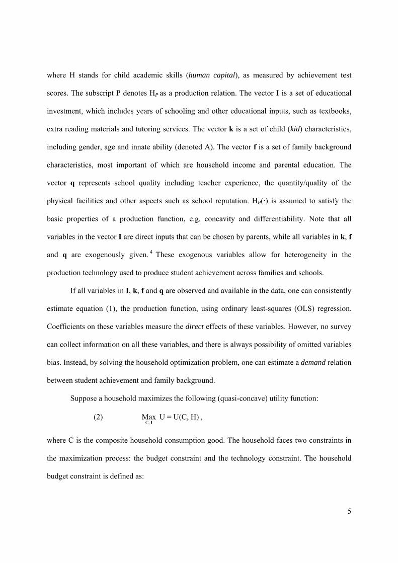
where H stands for child academic skills (human capital), as measured by achievement test

scores. The subscript P denotes HP as a production relation. The vector I is a set of educational

investment, which includes years of schooling and other educational inputs, such as textbooks,

extra reading materials and tutoring services. The vector k is a set of child (kid) characteristics,

including gender, age and innate ability (denoted A). The vector f is a set of family background

characteristics, most important of which are household income and parental education. The

vector q represents school quality including teacher experience, the quantity/quality of the

physical facilities and other aspects such as school reputation. HP(·) is assumed to satisfy the

basic properties of a production function, e.g. concavity and differentiability. Note that all

variables in the vector I are direct inputs that can be chosen by parents, while all variables in k, f

and q are exogenously given. 4 These exogenous variables allow for heterogeneity in the

production technology used to produce student achievement across families and schools.

If all variables in I, k, f and q are observed and available in the data, one can consistently

estimate equation (1), the production function, using ordinary least-squares (OLS) regression.

Coefficients on these variables measure the direct effects of these variables. However, no survey

can collect information on all these variables, and there is always possibility of omitted variables

bias. Instead, by solving the household optimization problem, one can estimate a demand relation

between student achievement and family background.

Suppose a household maximizes the following (quasi-concave) utility function:

(2) C,

Max U = U(C, H)I

,

where C is the composite household consumption good. The household faces two constraints in

the maximization process: the budget constraint and the technology constraint. The household

budget constraint is defined as:

6

(3) C p I mj jj

,

where Ij is the j-th element of the educational input vector, I, pj is the corresponding j-th element

in the price vector, p, and m is the total amount of monetary resources available to the

household. The technology constraint is defined by equation (1).

Solving problem (2) subject to constraints (1) and (3) yields the following demand

functions:

(4) C C ( , m; , , ) p k f q ,

(5) I I ( , m; , , )j j p k f q .

where equation (4) is the demand function for household consumption, and equation (5) is the

demand function for the j-th educational input. 5 Substituting (5) into equation (3), we obtain the

demand function for child achievement:

(6a) H H ( ( , m; , , )); , , )P I p k f q k f q .

Because elements in I are functions of the same set of exogenous variables, (k, f, q), equation

(6a) can be expressed as the following equation:

(6b) H H ( , m; , , )D p k f q .

Since equation (6b) expresses H as a function of only exogenous variables, it is a reduced-form

demand equation (as opposed to the structural relationship in equation (1)). The subscript D

denotes HD as a demand function. The reduced-form demand function is attractive for two

reasons. First, from the above derivation, one can see that the reduced-form relationship

characterized in equation (6b) takes into account the behavioral adjustments (through the

optimization process) to I in response to exogenous changes in any exogenous variable in (p, m,

5 A set of equation (5) has been estimated by Brown (2006) using the same data set used in this paper.

7

k, f, q), while holding others constant. To the extent that many governmental intervention

programs will lead to behavioral adjustments, equation (6b) is probably the most relevant for

policy makers (Blau 1999). Second, the data requirement for estimating a reduced-form demand

function is much less demanding for estimating a production function. Because all inputs I have

been substituted out, and thus the estimation is less likely to suffer from omitted variable bias.

Thus, equation (6b) is the key relationship of interest in this paper.

A simple linear approximation of equation (6b) can be written as:

(7) H αA ε xβ qη ,

where x = (p, m; k, f) is the matrix of all exogenous variables (except for ability A). A is child

ability and q is the vector of school quality. They are listed separately from x because they are

the sources of potential biases in estimation that will be discussed in more details in section 3

below. and ε is the error term that includes factors that have predictive power of H but are not

collected in data. One important example relevant to this paper is the measurement errors in A

and x variables. Equation (7) is the statistical model for the demand for student achievement that

will be estimated below. If equation (7) is a good approximation of equation (6b), and if we have

all data on variables on the right hand side of equation (7), we can consistently estimate the

effects of the right hand side variables in equation (7).

3. Identification Issues

Even when estimating a reduced form equation such as equation (7), careful econometric

analysis would be needed in order to consistently estimate the effects of the exogenous variables.

8

This section discusses identification issues that are raised by potential omitted variables and

measurement error. The next section presents our strategies to tackle these identification issues.

Unobserved school quality. Although they are often treated as inputs in education

production, school quality variables (q) cannot be substituted out in equation (6b) because they

are not choice variable for parents. Many empirical studies attempt to assess the effects of school

quality on student achievement, or simply to control for them, by including a list of school

characteristics that measure some dimensions of school quality. However, many dimensions of

school quality could affect student achievement. Hence it is likely that in most studies there are

always some school quality variables that are omitted, often because they are unobserved. By

comparing prospective estimates and retrospective estimates using data in Kenya, Glewwe et al

(2004) find evidence of omitted school quality variables bias, even when controlling for other

observed school quality variables.

The failure of controlling for omitted school quality variables will not only bias the

estimated effects of observed school quality variables, but could also lead to biased estimates of

the effects of variables in x. This is especially possible in the rural China case, given the

decentralization of funding structure of the basic education sector in rural areas. Schools in more

wealthy areas are probably of better qualities because local communities (consist of wealthy

households) in more wealthy areas probably have more capacity to invest in schools. Since

household income may be correlated with school quality, the omission of variables that measure

school quality may also bias the coefficient on variables that measure household income.

Unobserved Child Ability. Child innate ability can never be perfectly observed. The

omission of child innate ability could lead to upward biases on the estimated impacts of family

background characteristics (see e.g., Behrman and Rosenzweig 1999, among others). The

9

omitted variable bias arises because child innate ability A and family background f are often

correlated. For example, A is positively correlated with f through the genetic link between child

ability and parental ability and the effect of parental ability on f.

Measurement error in Ability measures. In attempts to control for unobserved child

ability, many studies have used some measures of the innate ability, most often intelligence test

scores, to proxy the true innate ability. For example, Kingdon (1996) used Raven’s Coloured

Progressive Matrices test score as a proxy of innate ability and replaced A directly with the

Raven’s score in the regression. However, none of the currently available measurements can

perfectly measure the true innate ability. In fact, any ability measures might reflect the influence

of environmental factors (American Psychological Association 1995). In other words, these

ability measures are at best imperfect proxies for the true innate ability. Although the use of the

imperfect proxies can, to some extent, reduce omitted variable bias, it will probably lead to

additional problems because they are error-ridden and the inclusion of them may contaminate the

estimates on other explanatory variables. This paper uses a cognitive development measure score

(CDM; see the data section below for a description) to measure child innate ability, and it will

also likely to have measurement error problems that need to be appropriately dealt with.

Suppose CMD measures the true ability A with measurement error e, as follows:

(8) CDM = A + e.

Simple algebra yields A = CDM e . Thus, using CDM as a proxy for A, the actual equation

being estimated is

(7a) H αA ε

+ α CMD α e + ε

xβ qη

xβ qη.

Whether measurement error e will cause problems in estimation depends on the

correlation between CDM and e (Wooldridge 2002). If e is correlated with the true ability A but

10

not its measure CDM, OLS will produce consistent (but not efficient) estimates of all the

coefficients in (7a). But if e is correlated with CMD, but the true ability, the existence of e will

likely cause bias in estimates of all coefficients. Unfortunately, in the context of this paper, e is

very likely to be correlated with CMD, i.e. Cov (CDM, e) ≠ 0. This leads us to the classical

error-in-variable (CEV) case. By standard econometric theory, in the CEV case, the ordinary

least squares regression of H on x, CMD and q generally gives inconsistent estimates of all

coefficients (Wooldridge 2002).6

4. Identification Strategy

4.1. The fixed-effects-instrumental-variable approach (FE-IV)

Since the focus of this paper in on the family side, a simple method to control for unobserved

school quality is simply to use the fixed effects estimator at school levels. Take equation (7) for

example, for the i-th student in the k-th school, the achievement demand function can be

rewritten as,

(7b) H αA ε

SC αA ε

ik ik k ik ik

ik k ik ik

x β q η

x β

The vector of school quality, qk, are constant across all students in school k. The entire set of qk,

together with its coefficient vector η, can be pooled into a school-specific constant, SCk (= qkη).

Then, the usual fixed effects estimation procedure applies. The fixed effect estimator is attractive

because it allows x to be correlated with unobserved q variables since the latter are included in

the regression through SCk. Note that the term SCk captures the effects of all school level

characteristics that do not vary within school k, both observed and unobserved.

11

One still needs to control for the unobserved child ability Aik in equation (7b) above, even

when unobserved school quality have been controlled for using school fixed effects. Since this

paper uses CDM to proxy the unobserved innate ability, the identification issues caused by

imperfect proxy for child ability discussed in the above section must be addressed here. Our

approach is to treat CDM as an indicator, instead of a proxy variable, of the true innate ability,

and then apply standard IV procedures to this indicator.7 This IV approach is proposed by

Griliches and Mason (1972) and also applied in Blackburn and Neumark (1992).

With school fixed effects being controlled, equation (7a) becomes:

(7c) ik ik ikH = SC α CDM α e + εik ik k x β

With unobserved school quality being controlled for, consistent estimates of the effects of x

variables can then be obtained if valid instrumental variables are available for CDMik. The set of

suitable IV used in this paper is described in the next subsection.

4.2. Famine in China, 1958-1961 and the Famine-Generated IVs

The Famine. Instrumental variables are usually difficult to find. But history helps. A

natural experiment generated by the Great Famine in China, 1958-1961, provides candidates for

the IV needed. The famine resulted from the agricultural crisis in 1958 and the following

political decisions regarding food allocation.8 The national grain production plunged by 15

possible approach can be found in the Ghana study by Glewwe and Jacoby (1994). The authors extracted an innate ability factor as a household fixed effect, using parental ability measures. In other words, the IQ score variable, i.e. the Raven score of the child, is instrumented by using father and mother’s Raven’s scores and other exogenous variables. Note that this approach is valid only if measurement errors in parental ability and child ability are uncorrelated. Also, because parental ability measures are not available in the data set used in this paper, other possibly suitable IVs are needed. 7 Detailed analysis of the causes of this famine can be found in Lin (1990), Lin and Yang (1998), Lin and Yang (2000), among others. 8 Indeed, Lin and Yang (2000) argue that food entitlement might be the fundamental cause of the famine.

12

percent in 1959 from its peak of 200 million tons in 1958. It declined by another 15 percent in

1960 and stayed flat in 1961 (State Statistical Bureau 1991). In order to deal with the food

shortage caused by the sharply decreased agricultural output, food allocation policies were

established during this period that gave urban grain supplies higher priority over rural localities.

To guarantee the success of the Great Leap Forward in 1958, Chairman Mao’s ‘One Chessboard’

speech in the spring of 1959 reaffirmed the urban-biased food allocation policy. This exacerbated

the shock of original output decline in the rural area (Lin and Yang 2000).9 .

The famine in 1958-1961 is now recognized as the worst in human history. It has been

estimated that the famine caused deaths of some 30 million of people and lost births of more than

30 million, mostly in rural areas (Ashton et al. 1984). Gansu province, the study area in this

paper, was seriously affected by the famine and the urban-biased policies that followed. The

administration extracted 361 thousand tons of grain from Gansu to support the urban food supply

between 1959 and 1960 despite the food shortage in the province (Walker 1984). At the same

time, the rigorously implemented residence registration (Hukou) system prevented rural residents

from migrating to urban areas where food shortage was not as dire. As a consequence, death

rates increased dramatically in Gansu from 11.1 ‰ in 1957 to 21.1‰ in 1958 and then peaked at

41.3 ‰ in 1960. The death rate in Gansu in 1958 was the third highest among all 28 provinces

for which data were available.

The Famine-Generated IV. It is clear that the famine cohort, people who were born

during or slightly before the famine period (i.e. people who spent their early childhoods during

the famine) and survived could be a very different cohort from the rest of the population in

Gansu. In particular, people in the famine cohort might have higher ability endowment than

13

those who did not survive and those who were born long after or long before the famine because

the famine “selected” out people with higher ability.10

In addition to the selection effect, the famine can also have a somewhat offset effect on

parents’ ability through poor prenatal nutrition intake. Recent studies on the long-term impacts of

the famine (e.g., Chen et al. 2007) indicates that people born during the famine period have

significantly lower heights than they would otherwise have had, which implies low nutrition

intakes during the famine. Early prenatal nutrition has been found to be essential in human brain

development. For example, Villar et al. (1984) found that infants whose head growth slowed due

to poor prenatal nutrition before 26 weeks of gestation (as measured by ultrasound) grew slower

than otherwise, and scored lower in mental performance in preschool years. Similarly, one would

expect the famine-born cohort to have lower ability than they would otherwise. This nutrition

effect could offset the selection effect the famine has on ability.

If a subset of the parents of the sample children belongs to the famine cohort, then famine

can serve as an IV for three reasons. First, there is a large literature showing that parents’ innate

ability is closely correlated with their children’s innate ability. Second, since the famine affects

parents’ ability, either through the selection effect or through the poor prenatal nutrition effect,

the famine is likely to be correlated with children’s ability. Third, because the famine can be

treated as a natural experiment, the variation in children’s innate ability that is associated with

the famine is exogenous and uncorrelated with the error term. Therefore, the famine can serve as

an instrumental variable for children’s innate ability. We create the instrumental variable using

that there is no contradiction between this argument and that in Chen et al. (2007). Famine could not only select out people with high endowment, but also affect their lives badly ever since. The idea here is that, their high endowment could have been masked by the long term negative impact of famine. Such endowment could still be transmitted to their children, however. 10Due to reasons such as migration out of Gansu province and child death, the total number of sampled children interviewed in 2004 is 1912.

14

parents’ birth year information: the total number of parents that were born and then survived

their early childhood during the famine.

5. Data

The data used in this paper come from the Gansu Survey of Children and Families

(GSCF). The survey follows 2000 sample children11 over years (2000, 2004 and 2007) in Gansu,

a poor province located in northwestern China. During the 2000 survey, a stratified sampling

strategy was first used to select 20 counties from all non-urban, non-Tibetan counties in the

province. Within each of the 20 counties, 5 villages were then selected. Within each of the 100

sample villages, 20 children were then randomly selected from the full cohort of nine to twelve

year-old children. Separate questionnaires were administered to the sample children, their

parents, local village leaders as well as to teachers and principals of the schools the sample

children enrolled in at the time of the survey.

Since the focus of this paper is academic achievement in basic education, a sub-sample of

children who were enrolled in grades 1-9 (excluding high school students in 2004) is used. One

reason is that basic education is compulsory while high school education is voluntary. Many

aspects of high school education, e.g., curriculum, cost12 and funding structure13 and motivation

hina, high school tuition is not free, while in many areas basic education is claimed to be free of tuition. 12 High schools in China are funded by county governments, while primary schools and middle schools are funded by township governments and local communities. 13 See Zhao and Glewwe (forthcoming) for an analysis of the determinants of the dropout decisions of these children.

15

of teachers and students, are different from that of basic education. In fact, about 250 children in

this sample have dropped out of school before they reach high school education.14

The dependent variable, child academic skill, is measured by math test scores. In 2004, a

math test was administrated to all sampled children. The tests were designed by experts at the

Gansu Educational Commission to cover the range of official primary school curriculum. To

ensure that the tests assessed an appropriate range of knowledge given the child’s education,

separate exams were given to children in different grades. Those sample children that were

interviewed in 2000 but dropped out before 2004 also took the tests in 2004. Tests that were

equivalent to the highest grade they have ever attained were given to them. The test scores are

then adjusted to be comparable. The inclusion of these children eliminates sample selection

biases caused by dropping out of school. Note that for the children who have dropped out of

schools, there will not be any information school available in the 2004 panel.15 Our strategy is to

replace school codes by the village codes for these children in our data. This strategy can control

for school fixed effect well because each village in rural Gansu usually have one primary school

and one lower-secondary school, and China’s policy on basic education enrollment is based on

locality of residence.

The most important family background variables are household income and parental

education. In household surveys, measures of household income are often collected by asking

respondents to report sources and amounts of income, which is subject to measurement error

caused by reporting error (Deaton 1997). Household expenditure would be a better measurement

of household income. However, since measurements of household expenditure often come from

her possible way is to replace school codes in 2004 by school codes in 2000. But one caveat of this approach is that many dropped out children have finished middle school education, which means the schools they attended in 2000 were their primary schools.

15 Inde

16

respondents’ recalling of expenses, they are also susceptible to measurement error unless

respondents keep a diary of daily consumption. To deal with measurement error in expenditure

data, the log value of durables per capita in 2000 is used as an instrumental variable. During the

survey, the enumerators conducted the interviews in the household residence calculated the value

of durables, and thus the measurement error in the value of durable is unlikely to be correlated

with the measurement error in household expenditure reported by household members.

Additionally, since educational investment is a medium or long term (probably 5-10 years)

decision, it is probably better explained by long term household resources instead of current

yearly household resources. Using the value of household durables in 2000 as an instrument for

household expenditure is similar to exacting a long term wealth component from the current

household resource measure. In most of the regressions below, household expenditure is

instrumented by the value of durables in 2000.

Parental education has been the focus in many empirical studies on child human capital

outcomes. In addition to ask the highest degree completed by the parents in most household

surveys in China, how many years were spent in pursuing the highest degree was collected. For

example, many parents spent two years, instead of three years, in middle schools, due to the

education policy in the 1970s. Hence, the years of schooling calculated in this sample will be

more precise than in most household surveys in China.

Child characteristics include gender and child age measured in month. Squared age is

also added in order to capture the nonlinear effect of age on academic skills. More importantly,

we also include child ability. A cognitive development test was administrated to each sample

child in 2000 when they aged 9 to 12. Scores of this cognitive test is used to measure child innate

ability.

17

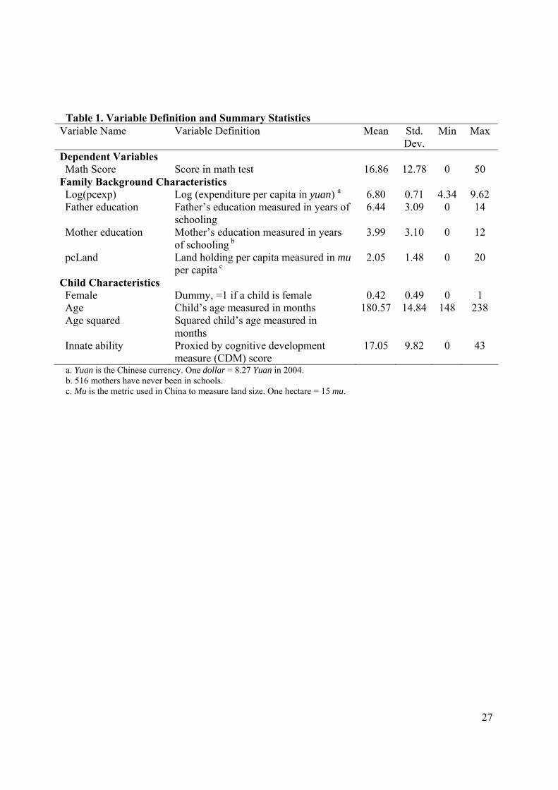
Table 1 summarizes definitions and summary statistics of variables used in the empirical

analysis.

6 Empirical Results

6.1. Potential bias: Omitted ability variable vs. Measurement error in CDM score.

Table 2 summarizes the empirical results for estimating a variety of equation (7), the reduced

form demand function for math achievement. At the same time, comparison across specifications

facilitates the investigation of potential bias caused by either the omitted innate ability or

measurement error contained in the ability measure CDM. Since this paper makes no attempt to

estimate the effect of school quality variables on math achievement, all specifications in table 2

control for school fixed effects. The main message in this sub-section is that although adding an

ability measure as a proxy for child ability reduces omitted ability bias to some extent,

measurement error in the ability measure causes new problems.

The first half of table 2 (column 1-2) does not control for child ability. The only

difference between these two specifications is that household expenditure in the second (column

2) is instrumented by the log value of durables in 2000, while in the first specification (column 1)

it is treated as exogenous, i.e., not containing any measurement error. The comparison of the

estimation results in these two specifications indicates the need to instrument household

expenditure. 16 Thus, in all other specifications (column 2-4), per capita household expenditure is

instrumented by the log value of durables per capita in 2000.

The second half of table 2, columns (3) and (4), controls for child innate ability, but with

different methods. The specification in column (3) uses CDM score as a proxy variable for

18

ability A and directly replaces A in the regression. In the last specification (column 4), the CDM

score is instrumented by the IV generated by the famine that indicates the number of birth

parents who were born and then survived the famine.17

The following analysis investigates the potential bias by comparing the coefficient

estimates from the baseline regression column (2) with those from column (3) and (4).

Consistent with the finding in Behrman and Rosenzweig (1999), among others, the omission of

child innate ability leads to upward ability-bias on the estimated impact of family income. For

example, the comparison of column (2) and column (4) indicates that household income effect is

overestimated. The coefficient estimate on the log value of expenditure per capita in column (1)

is 3 points higher than the consistent estimate in column (4). Interestingly, the effect of father’s

education is underestimated (by about one third of the size of the consistent estimate in column

(4)) in column (2). This suggests that there might be some interaction effects between child

ability and family background variables, which will be discussed below.

In attempts to remove omitted ability bias from omitting ability, CDM score is used to

proxy ability in the specification in column (3). The results clearly suggest that CDM score is

likely to measure ability A with a substantial amount of error. First and mostly significantly, the

results clearly indicate the existence of attenuation bias in the coefficient estimate on A when it

is proxied by CDM score. Compared to the result from the column (4), where CDM score is

instrumented by the famine-generated IV, the magnitude of the estimate in column (3) is less

than one third of size of the consistent estimate in column (4).

In summary, by comparing results from estimating different specifications that differ in

the approaches to deal with estimation problems, we show the biases could arise if one does not

17The significant predictive power of IV on the endogenous variables in the first-stage regressions (column 1 and 2 in Table 3) indicate the validity of our IV. In particular, the F-statistic of the famine-IV is close to 10, the rule of thumb for valid instrument variables.

19

control for child ability. In addition, if ability is not appropriately controlled for, problems persist.

Even if an ability measure, e.g., CDM score in this paper, is available, replacing A with CDM

score directly might cause other biases if CDM score contains a certain amount of error.

6.2. The main effects of family background and child characteristics

As expected, family background and child characteristics play important roles on student

math achievement (Table 2, column 4). However, not all their roles are consistent to common

findings in the literature. One striking finding from comparing income effects in column (2) and

(4) is that strong household income effects found in previous literature might be simply

reflecting the effects of child innate ability. Strong positive income effect is found in column (2)

where child innate ability is left in the error term. Since household expenditure is in log scale, a

ten percent increase in household expenditure is associated with 0.4 points increase in math

achievement, which is lager than the effects of increasing father’s education by one year. But

when child innate ability is appropriately controlled for in column (4), income effect drops

greatly and becomes insignificant at any conventional level. Meanwhile, a strong effect of innate

ability on math achievement is found. Also, even when an ability measure is used to proxy

unobserved child ability (column 3), income effect is still overestimated: although the income

effect decreased somewhat when CDM is added in column (3), it is still significant at 10% level.

The second interesting finding is that the most significant family background variable is

father’s education, but not mother’s education which has long been found to be a more

significant determinant than father’s education on many measures of child human capital

outcomes in the literature. In fact, mother’s education plays almost no role in child math

achievement (table 2, column 2-4) in the linear specifications of equation (7).

20

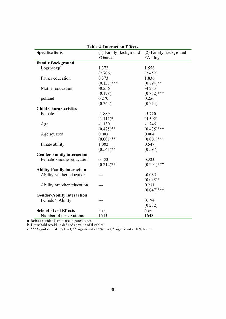
6.3. Interaction effects: Gender and Family Background

The above findings are plausible only when the specification in equation (7) is correct.

Table 4 explores more possibilities by introducing interaction terms between family background

variables and child characteristics. This sub-section considers the interaction between family

background and child gender, which is suggested by Brown and Park (2002)’s findings on

gender effect in China. Household expenditure and parental education are interacted with the

gender dummy. 18 No significant income effect or its interaction effect with child gender is found.

The interaction between father’s education and child gender are also never significant. Thus,

only the interaction between mother’s education and child gender is kept in the regression

reported in table 4.

The main finding is that although both father’s education and mother’s education have

significant impacts on child math achievement, the effects of father’s education and mother’s

education differ. Other things being equal, an additional year of father’s education is associated

with about 0.4 point increase in math achievement, for both boys and girls. In contrast, mother’s

education matters only for girls, and the effect of mother’s education is slightly higher than that

of father’s education.

As has been commonly documented in research on developing countries, gender gap is

also found in table 4 when interaction effects are considered. First, girls scored lower than boys

if their mothers’ years of schooling are lower than 4.3 years, which is higher than the mean level

of mothers’ education (i.e., four years; see table 1) in this sample.19 Second, mother’s education

18 The interaction between household expenditure and child gender is instrumented by the interaction between the value of durable in 2000 and child gender. 19 The marginal effect of being a girl is -1.89 + 0.43× mother’s education. So if mother’s education is more than 4.3 years, the marginal effect of being a girl is positive.

21

plays an important role in raising girls’ math achievement but not in raising boys. Along with

these two findings, the fact that more than 500 mothers in the sample have never been to school

suggests that females may have been discriminated against in education for more than one

generation. Given that family background, school quality and child ability have been controlled

for, one possible explanation for the differential effects of mother’s education on boys’ and girls’

math achievement is that more-educated mother might provide a household role model for girls.

In other words, more-educated mothers provide high motivation for their daughters, who would

be discriminated against otherwise, to study hard.

6.4 Interaction Effects: Ability and Family Background

Strong ability effect on math achievement has been found above (table 2, column 4; table

4, column 1): Children who with the ability to score one point higher in CDM than average will

score 1 point higher in math achievement, other ting being equal. However, this finding is not

helpful in providing evidence for government to design intervention programs.20 Therefore, it

might be more useful to investigate the interaction effects between child ability21 and family

background variables. The results are summarized in table 4, column 2.22

Again, no income effect (or its interaction effects with child characteristics) is found.

Also, the three way interaction, child gender-ability-family background has little predictive

power on student math achievement. Importantly, differential effects of parental education are

again found across innate ability levels. For example, the effect of father’s education decreases

20 It is helpful in the sense that it suggests the strong household income effect might be picking up the ability effect. 21 The fitted value from the first-stage regression of CDM in table 3 is used as the proxy for child ability. 22 The interaction between household expenditure and child ability and the three way interaction among household expenditure, child gender and child ability are not significant and are thus dropped from the regression.

22

as child ability increases. In other words, the effect of father’s education is higher for a child

with lower innate ability than a child with higher innate ability. On the contrary, the effect of

mother’s education has higher an impact for children with higher ability. These suggest different

educational investment strategies adapted by fathers and mothers. While fathers might adapt

compensating strategy, i.e., invest more in less able children, mothers do the opposite. Although

the arguments that fathers and mothers adapt different strategy seems strange, they do not lack of

empirical support. For example, for the same sample of children, Brown (2006) finds that

father’s education has a significantly negative effect on the amount of extra reading material

purchased for children with higher ability, while mother’s education has a small positive

impact.23 This pattern reverses in the number of times parents discuss their children’s

performance in school with their school teachers. These findings, i.e., the differential effects of

father’s and mother’s education across child gender and ability level, suggest the need for further

research on household structure in rural China.

7. Summary and Conclusions

This paper investigates the determinants of academic skills (as measured by math test

scores) acquired in basic education (i.e. grades 1-9) for a sample of rural children (aged 9-12 in

2000) from Gansu, a poor province in China. In order to obtain consistent estimates of the

effects of family background, we developed an instrumental variable approach to deal with the

potential econometric problems caused by the unobserved child ability variables. Unobserved

school quality is controlled by a set of school fixed effects. An error-ridden measure of child

ability, the score of a cognitive ability test, is available to (imperfectly) proxy child ability. To

23 Brown (2006) uses the same CDM as that in this paper. But he does not use the continuous measure of CDM, nor does he address the measurement error problem in it. Instead, he creates a dummy for children who scored higher than average.

23

deal with measurement error in this ability measure, a variables indicating the number of the

parents who were born around the Great Famine in China, 1958-1961, are used as our

instrumental variables.

This paper has two major findings, using the famine-IV approach. The first is the

possibility that the strong household income effect found in the literature might merely reflect

the effect of child ability. This paper shows clearly that income effect will be overestimated if

child ability is omitted or if an ability measure is available but it contains a certain amount of

measurement error.

The second finding is the significant effects of parental education, child characteristics

and their interactions on math achievement. Father’s education has significant impacts on both

boys’ and girls’ academic skills, while mother’s education is only significant for girls. Also,

child gender matters greatly. The gender effect, together with the fact that more 500 mothers do

not have any formal education, suggests that gender bias have long existed in formal education in

rural China. Furthermore, the effects of father’s education and mother’s education differ across

ability level. While father’s education has a bigger impact for children with lower ability,

mother’s education has a bigger impact for more able children. These findings suggest the need

for further research on household structure in rural China.

References

Ashton, Basil, Kenneth Hill, Alan Piazza, and Robin Zeitz. (1984). “Famine in China, 1958-61.”

Population and Development Review 10(4): 613-645

Behrman, Jere R., and Mark R. Rosenzweig. (1999). “‘Ability’ biases in schooling returns and

twins: a test and new estimates.” Economics of Education Review 18(2):159-67

Behrman, Jere R., and James, C. Knowles (1999). “Household Income and Child Schooling in

Vietnam.” World Bank Economic Review 13(2): 211-56

24

Blackburn, McKinley, and David Neumark. (1992). “Unobserved Ability, Efficiency

Wages, and Interindustry Wage Differentials.” Quarterly Journal of Economics

107(4):1421-36

Blau, David, M. (1999). “The Effect of Income on Child Development.” The Review of

Economics and Statistics, 81(2): 261-276

Brown, Philip H. (2006). “Parental Education and Investment in Children's Human Capital in

Rural China.” Economic Development and Cultural Change 54(4):759–89

Chen, Yuyu and Li-An Zhou. (2007). “The long-term health and economic consequences of the

1959–1961 famine in China”, Journal of Health Economics 26 (4): 659-81

de Brauw, and Scott Rozelle. (2008). “Reconciling the Returns to Education in Off-Farm Wage

Employment in Rural China”. Review of Development Economics 12(1): 57-71

Deaton, Angus. (1997). “The Analysis of Household Surveys.” The Johns Hopkins University

Press.

Duflo, Esther. (2001) “Schooling and Labor Market Consequences of School Construction in

Indonesia: Evidence from an Unusual Policy Experiment” American Economic Review

91(4): 795-813

Glewwe, Paul. (1996). “The relevance of standard estimates of rates of return to schooling for

education policy: A critical assessment” Journal of Development Economics 51(2):267-

90

Glewwe, Paul. (2002). “Schools and skills in developing countries: Education policies and

socioecomic outcomes”. Journal of Economic Literature 40(2):436-82

Glewwe, Paul, and Hanan G. Jacoby. (1994), “Student Achievement and Schooling Choice in

Low-Income Countries: Evidence from Ghana.” Journal of Human Resources 29(3):

843-64

Glewwe, Paul, Hanan G. Jacoby, and Elizabeth M. King. (2001). “Early childhood nutrition and

academic achievement: a longitudinal analysis.” Journal of Public Economics 81(3): 345-

68

Glewwe, Paul, and Elizabeth M. King. (2001). “The Impact of Early Childhood Nutritional

Status on Cognitive Development: Does the Timing of Malnutrition Matter?” World

Bank Economic Review 15(1): 81-113

Gleww, Paul, and Michael Kremer. (2006). “Schools, Teachers, and Education Outcomes in

25

Developing Countries” In Hanushek, Eric A., and Finis Wlech (Eds.), Handbook of the

Economics of Education, vol. 2. Elsevier

Glewwe, Paul, Michael Kremer, Sylvie Moulin, and Eric Zitzewitz. (2004). “Retrospective vs.

prospective analyses of school inputs: the case of flip charts in Kenya” Journal of

Development Economics 74:251-68

Griliches, Zvi and William M. Mason. (1972). “Education, Income, and Ability.” Journal of

Political Economy. 80, no. S3.

Griliches, Zvi. (1977). “Estimating the Returns to Schooling: Some Econometric Problems.”

Econometrica 45(1): 1-22

Hanushek, Eric A. (1997). “Assessing the Effects of School resources on Student Performance:

An Update.” Educational Evaluation and Policy Analysis 9(2): 141-64

________. (2003). “The Failure of Input-Based School Policies” Economic Journal 113: F64-98

Haveman, Robert, and Barbara Wolfe. (1995). “The Determinants of Children’s Attainments:

A Review of Methods and Findings.” Journal of Economic Literature 33(4):1829-78

Heckman, James J. (2003). “China’s Investment in Human Capital.” Economic Development and Cultural Change 51:795–804

Jolliffe, Dean. (1998). “Skills, Schooling, and Household Income in Ghana” World Bank

Economic Review 12 (1): 81-104

Kindon, G. (1996). “The quality and efficiency of public and private schools: A case

study of India.” Oxford Bulletin of Economics and Statistics 58(1): 55-80

Lin, Justin Yifu. (1990). “Collectivization and China's Agricultural Crisis in 1959-1961.” Journal of Political Economy 98(6):1228-52

Lin, Justin Yifu, and, Dennis Tao Yang. (1998). “On the causes of China's agricultural crisis and

the great leap famine.” China Economic Review 9(2): 125-40

_______. (2000). “Food Availability, Entitlements and the Chinese Famine of 1959-61”.

Economic Journal 110(460):136-58

Plug, Erik, and Wim Vijverberg. (2005). “Does Family Income Matter for Schooling Outcomes?

Using Adoptees as a Natural Experiment.” Economic Journal 115: 879-906

Psacharopoulos, G. (1985). “Returns to education: A further international update and

Implications.” Journal of Human Resources 20(4): 583-604

____________. (1994). “Returns to investment in education: A global update.” World

Development 22: 1325-1344

26

Tan, J.-P., Lane, J., and Coustere, P. (1997). “Putting inputs to work in elementary schools:

What can be done in the Philipines?” Economic Development and Cultural Chang 45(4):

857-79

Tsang, Mun C. (1996). “Financial Reform of Basic Education in China.” Economics of

Education Review 15(4):423-44.

Villar, J., V. Smeriglio, R. Martorell, C. H. Brown, and R. E. Klein. (1984). “Heterogeneous

Growth and Mental Development of Intrauterine Growth-Retarded Infants During the

First 3 Years of Life” Pediatrics 74(5): 783-91

Walker, Kenneth R. (1984). “Food grain procurement and consumption in China.” Cambridge

University Press. Cambridge and New York.

Wooldridge, Jeffery M. (2002). Econometric Analysis of Cross Section and Panel Data. The

MIT Press. Cambridge, Massachusetts.

Yang, D. Tao. (1997a). “Education in Production: Measuring Labor Quality and Management”

American Journal of Agricultural Economics 79(3): 764-72

Yang, D.Tao. (1997b). “Education and Off-Farm Work” Economic Development and Cultural

Change 45: 613–32

Yang, D. Tao. (2004). “Education and allocative efficiency: household income growth during

rural reforms in China.” Journal of Development Economics 74(1):137-62

Zhao, Meng, and Paul Glewwe. “Determinants of Education Attainment: Evidence from Rural

Area in Northwest China.” Economics of Education Review (forthcoming)

Zhao, Yaohui. (1997). “Labor Migration and Returns to Rural Education in China” American

Jouranal of Agricultural Economics 79: 1278-87

Zhao, Yaohui. (1999). “Labor Migration and Earnings Differences: The Case of Rural China.”

Economic Development and Cultural Change 47(4):767–82

27

Table 1. Variable Definition and Summary Statistics

Variable Name Variable Definition Mean Std. Dev.

Min Max

Dependent Variables Math Score Score in math test 16.86 12.78 0 50

Family Background Characteristics Log(pcexp) Log (expenditure per capita in yuan) a 6.80 0.71 4.34 9.62 Father education Father’s education measured in years of

schooling 6.44 3.09 0 14

Mother education Mother’s education measured in years of schooling b

3.99 3.10 0 12

pcLand Land holding per capita measured in mu per capita c

2.05 1.48 0 20

Child Characteristics Female Dummy, =1 if a child is female 0.42 0.49 0 1 Age Child’s age measured in months 180.57 14.84 148 238 Age squared Squared child’s age measured in

months

Innate ability Proxied by cognitive development measure (CDM) score

17.05 9.82 0 43

a. Yuan is the Chinese currency. One dollar = 8.27 Yuan in 2004. b. 516 mothers have never been in schools. c. Mu is the metric used in China to measure land size. One hectare = 15 mu.

28

Table 2. Results of Estimating Demand for Math Skills Dependent variable = Math test score

Specifications (1) (2) (3) (4) Ability Omitted Omitted CDM as proxy IV for CDMb

Estimator OLS 2SLSa 2SLS 2SLS Family Background

Log(pcexp) 0.964 (0.573)*

4.407 (2.121)**

3.443 (2.086)*

1.404 (2.683)

Father education 0.286 (0.110)***

0.241 (0.114)**

0.280 (0.111)**

0.363 (0.136)***

Mother education 0.130 (0.118)

0.025 (0.135)

0.005 (0.131)

-0.036 (0.146)

pcLand 0.438 (0.310)

0.329 (0.320)

0.315 (0.311)

0.288 (0.340)

Child Characteristics Female -0.821

(0.601) -0.693 (0.613)

-0.511 (0.596)

-0.126 (0.713)

Age -0.901 (0.430)**

-1.031 (0.443)**

-1.057 (0.430)**

-1.113 (0.471)**

Age squared 0.003 (0.001)***

0.003 (0.001)***

0.003 (0.001)***

0.003 (0.001)**

Innate ability --- --- 0.335 (0.043)***

1.044 (0.535)*

School fixed Effects Yes Yes Yes Yes R-squared 0.08 No of observations 1643 1643 1643 1643

a. Log expenditure per capital is instrumented by Log value of durables per capita in year 2000. b. CDM is instrumented by Famine-IV. c.* significant at 10%; ** significant at 5%; *** significant at 1%.

29

Table 3. First-Stage Regressions of Specification (5) in Table 2. Dependent variables (1)

CDM score in 2000 (2)

Log expenditure per capita

Instruments Log (durable per capita in 2000) 0.543

(0.224)** 0.169 (0.016)***

Number of Famine-born parents 2.319 (0.745)***

-0.018 (0.053)

Family Background Father education -0.087

(0.070) 0.007 (0.005)

Mother education 0.118 (0.075)

0.022 (0.005)***

pcLand 0.084 (0.196)

0.023 (0.014)*

Child Characteristics Female -0.548

(0.381) -0.033 (0.027)

Age 0.159 (0.272)

0.039 (0.019)**

Age squared -0.000 (0.001)

-0.000 (0.000)**

School Fixed Effects Yes Yes County Fixed Effects No No

R squared 0.08 0.11 Number of observations 1643 1643

a. Robust standard errors are in parentheses. b. Household wealth is defined as value of durables. c. *** Significant at 1% level; ** significant at 5% level; * significant at 10% level.

30

Table 4. Interaction Effects.

Specifications (1) Family Background ×Gender

(2) Family Background ×Ability

Family Background Log(pcexp) 1.372

(2.706) 1.556 (2.452)

Father education 0.373 (0.137)***

1.836 (0.794)**

Mother education -0.236 (0.178)

-4.283 (0.852)***

pcLand 0.270 (0.343)

0.256 (0.314)

Child Characteristics Female -1.889

(1.111)* -5.720 (4.592)

Age -1.130 (0.475)**

-1.245 (0.435)***

Age squared 0.003 (0.001)**

0.004 (0.001)***

Innate ability 1.082 (0.541)**

0.547 (0.597)

Gender-Family interaction Female ×mother education 0.433

(0.212)** 0.523 (0.201)***

Ability-Family interaction Ability ×father education --- -0.085

(0.045)* Ability ×mother education --- 0.231

(0.047)*** Gender-Ability interaction

Female × Ability --- 0.194 (0.272)

School Fixed Effects Yes Yes Number of observations 1643 1643

a. Robust standard errors are in parentheses. b. Household wealth is defined as value of durables. c. *** Significant at 1% level; ** significant at 5% level; * significant at 10% level.