A. Mathematical Tools

Most geodynamic processes are processes that change in space and time. One of the most important tools to describe such changing processes are differential equations. This chapter is therefore mainly concerned with the use and interpretation of differential equations. A few selected other important numerical tricks and basic rules are summarized towards the end of this chapter.

A.1 What is a Differential Equation?

The derivative (or: differential) dy/dx is a way to describe the change of y with respect to another variable x. It can be interpreted as the slope (or gradient) of the function y = f(x). If the slope of this function is constant between two points along the x axis, for example between x and x + Llx, then we need no derivative and we can write:

d. y(x + Llx) - y(x) gra lent = Llx . (A.1)

The numerator of the fraction on the right hand side of this equation is given by the difference between the y values of the function at the two points x and x + Llx. The denominator is given by the distance between the two points on the x axis between which the gradient is measured (Fig. A.1). Their ratio is the slope between the points x and x + Llx. If we consider a function where the slope is not constant between x and x+Llx, then eq. A.1 would give us only some mean of all the slopes of this function between the two points. However, the smaller we choose our Llx, the better will eq. A.1 describe the exact slope at point x. We can write:

y'(x) = dy = lim Llx -+ 0 (y(x + Llx) - y(x)) dx Llx

(A.2)

Eq. A.2 is the mathematical definition of a derivative. Note that we used a dash to indicate that y' is a derivative. This is a commonly used notation. The slope of a mountain road is a clear example to illustrate the meaning of slope. Assume that H describes the elevation of the road surface as a function

350

Figure A.I. Diagram illustrating the defini­tion of the first derivative of a function (thick curve) (eq. A.I and A.2). The slope of the thick drawn straight line may be accurately described by the ratio (y(x + .:1x) - y(x))/.:1x. The slope of the curved function at x is only moderately well approximated by this ratio. However, the smaller .:1x becomes, the better this approxi­mation will be to describe the slope at a single point

A . Mathematical Tools

of distance from the valley x: H = f(x). Then, the slope of the road is given by the first derivative of this function f~:

(A.3)

The units of this differential are mm- l . In short, it is dimensionless for this example. Familiar geological examples described by first derivatives (first differentials) of functions are the geothermal gradient, describing the change of temperature with depth (in °C m- I ), or cooling histories of metamorphic terrains that describe the change of temperature over time (in °C S-I).

The second derivative (or second differential) of a function describes how the slope changes. The familiar name of the second derivative is CUTvatuTe. It is often abbreviated with f:. In our example of a mountain road, the vertical curvature of the road is

" d(dH) d2H f = __ d_:r_ = --x dx dx2

(A.4)

and has the units of m/(m m-2 ), which is: m- I . It may be read as: "d two Hover dx squaTe". The scheme we have followed to go from first to second derivative may be followed to describe the third, fourth or higher derivatives of functions. Corresponding to the first two derivatives, the third derivative of a function describes the change of the curvature of the function and the fourth the curvature of the curvature and so on (Fig. A.2):

f~! and: f~"' (A.5)

In our example of a mountain road, the units of the third and fourth derivatives are m -2 and m -3, respectively. Be careful not to confuse these linear derivatives of the third and fourth order (in eq. A.5) with the non-linear first order deri vati ves (dH / dx ) 3 and (dH / dx) 4 (see below)!

A.l . What is a Differential Equation? 351

Figure A.2. A sine function as an example for the function Ix 0

and its first, second and third II

derivatives. At the maximum of 0

the function (point A), the slope

of the function is I~ = 0 and the curvature has a negative 0

" maximum: Ix = -1. Conversely, at the inflection point of the curve (point B), the slope has a minimum the curvature is zero 0 I: = O. At the minimum of the function (point C), the slope is also zero and the curvature has a maximum 0

0 2 3 4 5 6

A.I.1 Terminology Used in Differential Calculus

Order. The order of the highest derivative in a differential equation is called the order of the equation. For example, eq. 3.58 is a first order differential equation, eq. 3.6 or eq. 3.57 are second order differential equation eq. 4.42 is a fourth order differential equation. Fig. A.2 illustrates the meaning of derivatives of higher order using the example of a simple sine function.

Partial and Total Derivatives. A function may have several variables. For example, the elevation of a point H on the surface of the earth can be described as a function of two spatial coordinates in the horizontal directions x and y, but it may also be a function of time or any other variables that we deem of importance, say vegetation or lithology. If we consider the spatial dependence only, we may be in the situation to describe the elevation of our point as:

(A.6)

If we differentiate this function with respect to one of the variables only, then this is called a partial derivative. It describes the slope of the function in one spatial direction only. When forming a partial derivative with respect to one variable, then all other variables are kept constant during the process and are treated like any other constant of the equation. The symbol for the partial differential is 0 (say: "del''). However, "del" is no real Greek letter and should not be confused with o. The partial derivative of eq. A.6 after x is:

oH = 6x ox y=const.

(A.7)

352 A . Mathematical Tools

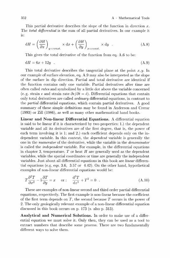
This partial derivative describes the slope of the function in direction x. The total differential is the sum of all partial derivatives. In our example it is:

(OH) (OH) dH = - x dx + - x dy . ax y=const. oy x=const.

(A.8)

This gives the total derivative of the function from eq. A.6 to be:

dH = 6x + 12y . (A.9)

This total derivative describes the tangential plane at the point x, y. In our example of surface elevation, eq. A.9 may also be interpreted as the slope of the surface in dip direction. Partial and total derivative are identical if the function contains only one variable. Partial derivatives after time are often called rates and symbolized by a little dot above the variable concerned (e. g. strain E and strain rate OE/Ot = i). Differential equations that contain only total derivatives are called ordinary differential equations, in contrast to the partial differential equations, which contain partial derivatives. A good summary of these simple definitions may be found in Anderson and Crerar (1993) or Zill (1986), as well as many other mathematical hand books.

Linear and Non-linear Differential Equations. A differential equation is said to be linear if it is characterized by two properties: 1.) the dependent variable and all its derivatives are of the first degree, that is, the power of each term involving it is 1; and 2.) each coefficient depends only on the in­dependent variable. In this context, the dependent variable is generally the one in the numerator of the derivative, while the variable in the denominator is called the independent variable. For example, in the differential equations in chapter 3, temperature, T or heat H are generally used as the dependent variables, while the spatial coordinates or time are generally the independent variables. Just about all differential equations in this book are linear differen­tial equations (e.g. eqs. 3.6, 3.57 or 4.42). On the other hand, hypothetical examples of non-linear differential equations would be:

or: (A.I0)

These are examples of non-linear second and third order partial differential equations, respectively. The first example is non-linear because the coefficient of the first term depends on T, the second because T occurs in the power of 2. The only geologically relevant example of a non-linear differential equation discussed in this book occurs on p. 173 (s. also p. 313).

Analytical and Numerical Solutions. In order to make use of a differ­ential equation we must solve it. Only then, they can be used as a tool to extract numbers that describe some process. There are two fundamentally different ways to solve them.

A.I . What is a Differential Equation? 353

• 1. Analytical solutions. Analytical or closed solutions of differential equa­tions may be found by integrating them. Let us consider as an example the description of a geotherm by

dT

dz 1.5 VZ· (A.ll)

There, T is temperature in °C and z is depth. This differential equation can be integrated without difficulty:

T = 3VZ+C . (A.12)

The integration constant C must be determined using boundary condi­tions. Eq. A.12 is said to be an "analytical solution of the differential equation eq. A.ll". If we assume (as our boundary condition) that the temperature at the earths surface is always zero and we assume a coordinate system where the surface is at z = 0, then this constant must be also zero: C = O. Now eq. A.12 can be used to calculate temperatures at any depth of our choice by inserting numbers for z. For example, for z = 100 000 m eq. A.12 gives T=949°C.

• 2. Numerical solutions. Numerical solutions of differential equations are used to extract numbers from differential equations without having to solve (integrate) them. With their aid we can arrive at the result that eq. A.ll describes a temperature of T = 949°C, at 100 km depth if the surface tem­perature is zero without having to solve the differential equation, i.e. without having to go from eq. A.ll to eq. A.12. However, numerical solutions are not exact. Numerical approximations are always only approximations and they are plagued by stability and accuracy problems (s. p. 358). The numerical so­lution of partial differential equations is a science on its own (sect. A.2, A.4). The two most important methods that are in use are the finite difference methods and the finite element methods.

The finite element method has the advantage that it is much more ele­gant to use it for the description of deformation on Lagrangian coordinates. The principal disadvantage of the finite element method is that it is quite a complicated method not amenable to the understanding of a field geologist.

The finite difference method has the enormous advantage that it is quite intuitive, easy to implement on a computer (even by inexperienced math­ematicians) and easily adaptable to many different problems. Its principal problems are those of instability, and that they are quite cumbersome when it comes to the treatment of discontinuous boundary conditions and deformed grids (sect. A.2).

• Advantages and disadvantages. Numerical and analytical solutions have both their advantages and disadvantages. The enormous advantage of nu­merical solutions is that they allow us to arrive at results without having to know enough differential calculus to be able to integrate the equation in

354 A . Mathematical Tools

question. In fact many geological problems can be simplified enough to be able to formulate them into an equation, but are too complicated so that an analytical solution even exists. In such cases, numerical solutions are the only way to obtain results.

Analytical solutions have the advantage that they are much more useful to understand the nature of a geological process. For example, eq. A.12 may be used directly to infer that the temperature in the crust rises with the square root of depth. If this model corresponds well with our observations in nature, then we can continue to think about the significance of this quadratic relationship. Such considerations are difficult with numerical solutions as they only deliver numbers.

Initial- and Boundary Conditions .

• Boundary conditions. When solving differential equations, boundary con­ditions are necessary in order to determine the integration constants. This is true for both numerical and analytical solutions. For differential equations of the first order we need one boundary condition, for those of the second order two and so on. The term boundary condition is exactly what it implies: it is a condition at the boundary of the model (s. sect. A.2.1). The most common types of boundary conditions are:

A prescribed value of the function at the model boundary (e. g. T = 0 at z = 0; s. eq. A.12), A prescribed gradient of the function at the model boundary (e. g. the heat flow boundary condition we used in sect. 3.4.1), A functional relationship between value and gradient at the model bound­ary (e. g. the constant heat content boundary condition used on p. 114).

Boundary conditions given by higher derivatives of functions are also pos­sible and play an important role when integrating differential equations of higher orders (s. sect. 4.2.2, eq. 4.42). In sect. A.2 we discuss how some of these boundary conditions may be implemented .

• Initial conditions. Initial conditions are necessary to determine the start­ing point of a model. For example, if we want to use the diffusion equation (eq. 3.6) to calculate the evolution of a diffusive zoning profile over time, then we must use a function T = J(z) at the time t = 0 from which we can start calculating. The nature of this function T = J(z) must be determined by a known initial condition.

A.2 The Finite Difference Method

The finite difference method makes use of the discretization of the derivative from eq. A.2. Instead of describing the differential dy/dx by the limiting value Llx -t 0, a finite value of Llx is used (i.e. eq. A.l is retained). For our

A.2 . The Finite Difference Method 355

explanation on the next pages we use Fig. A.3 showing the function T = f(x) and assume that this function is a temperature profile across a metamorphic terrain along the spatial axis x. Thus, we will use the variable T instead of the more abstract y that we have used up to now in this chapter. At the point Xi (labeled in Fig. A.3a by the dotted line) the function has the slope dT /dx. When using the method of finite differences, this slope is approximated by the discrete temperature difference at two different places with a finite distance to each other (a bit as we have already implicitly shown in Fig. A.I). There is many ways to formulate such a difference. In Fig. A.3b we can see that one way to formulate such a difference is:

dT Ti+1 - Ti Ti+1 - Ti dx ::::::i Xi+l - Xi = L1x .

(A.13)

The index i is just a description of the number of the grid point chosen here. Ti is the temperature at the "ith " point of a discrete grid of points. Ti+1 is the temperature at the next point of the grid, Ti - 1 at the previous point. The finite difference method used in eq. A.13 is called forward differencing method as we have calculated the temperature gradient at Xi using the temperature at Xi as well as the temperature at the next forward point on the grid (Fig. A.4). Some other simple examples of differencing schemes have the form:

dT Ti - Ti- 1 dT Ti+1 - Ti- 1

dx::::::i L1x or dx ::::::i 2L1x' (A.14)

For reasons that should now be obvious, these two methods are called backward differencing and central differencing schemes (Fig. A.4). • Differentiating with respect to time. All information we have discussed so far is generally applicable, regardless of what variable is described by x, y or T. However, the use of X has suggested that we imply spatial differentials. In order to discriminate between the numbering of grid nodes of spatial and temporal grids, the symbols "+" and "-" are common to describe the next

T T

------y(---------------: i ((x)

I "\ i

I

/'J.X

I ; x

Xi Xi-l Xi X'+l

a slope at a point b finite difference approximation

Figure A.3. Graphical illustration of the method of finite differences. In a the slope of the function f(x) at point Xi is accurately described by the touching tangent. Mathematically this slope is described by the differential dT /dx. In b the slope is approximated by the ratio of the differences of two temperature and two X values

356 A . Mathematical Tools

time step and the previous time step while i and i + 1 is used for the spatial grid stepping. Thus we can write:

dT T+ -T­ill ~ Llt (A.15)

In some books "j" and "j + I" are used to denote time steps. However , this should not be confused with spatially two-dimensional problems in which "i" subscripts are used for grid numbering in x direction and "j" numbering of grid steps in y direction .

• Approximations of derivatives of higher order. For the approximation of derivatives of the second or higher order we can use the same scheme as that for the first derivative (eq. A.13 , A.14) . For the second derivative we must form the ratio of the difference in slope at two different grid points with the distance Llx:

d2T d (~~) (Ti+~;Ti ) - ( Ti~;-l ) THI - 2Ti + Ti- 1 dx2 = ~ ~ Llx = Llx2 . (A.16)

From eq. A.16 we can see that, in order to formulate the difference between slopes at two point, the slope at point i was approximated once by forward differencing and once by backward differencing. This is necessary, as we want to calculate the curvature at point i from t he differences between the slopes of the curve as near as possible to it (i.e. in front of it and behind it). We can see that the curvature is described by the difference of slopes, just like we describe the slope by the differences between two function values .

• Solution of the diffusion equation using finite differences . If differential equations contain more than one variable (e. g. the diffusion equation (eq. 3.6), in which both spatial and temporal derivatives occur) it is necessary to com­bine several indices with each other. This may lead to apparently quite com­plicated formulations. Here we will follow the use of temporal and spatial

forward central backward

+ • • 1': + • ~ + • /I •

• • • • • <lI <lI <lI E • • • • E • • • • E • • • • .'" .'" .'" x x

.'I x space .J. space .J. .± space .± .±

F igure A .4. Schematic illustration of three simple methods of discretization in the finite difference method. The x axis of each diagram shows four discrete points of a one-dimensional spatial grid . Each dot is a temperature value at this point in space. The y-axis shows three different time steps of the calculation. In the three diagrams, the temperature at the third grid point (labeled by subscript i) is calculated by backward, forward and central differencing. In each diagram this calculation is for the values at the (as yet) unknown time step "+" from known information at time "-,,

A.2 . The Finite Difference Method 357

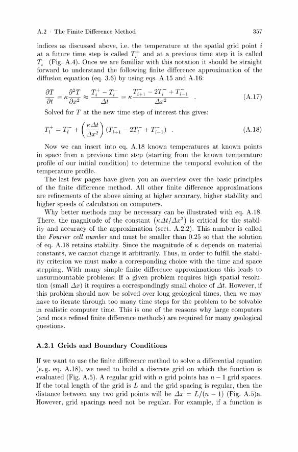
indices as discussed above, i.e. the temperature at the spatial grid point i at a future time step is called Ti+ and at a previous time step it is called Ti- (Fig. A.4). Once we are familiar with this notation it should be straight forward to understand the following finite difference approximation of the diffusion equation (eq. 3.6) by using eqs. A.I5 and A.I6:

(A.I7)

Solved for T at the new time step of interest this gives:

(A.I8)

Now we can insert into eq. A.I8 known temperatures at known points in space from a previous time step (starting from the known temperature profile of our initial condition) to determine the temporal evolution of the temperature profile.

The last few pages have given you an overview over the basic principles of the finite difference method. All other finite difference approximations are refinements of the above aiming at higher accuracy, higher stability and higher speeds of calculation on computers.

Why better methods may be necessary can be illustrated with eq. A.I8. There, the magnitude of the constant (",LltjLlx2 ) is critical for the stabil­ity and accuracy of the approximation (sect. A.2.2). This number is called the Fourier cell number and must be smaller than 0.25 so that the solution of eq. A.I8 retains stability. Since the magnitude of '" depends on material constants, we cannot change it arbitrarily. Thus, in order to fulfill the stabil­ity criterion we must make a corresponding choice with the time and space stepping. With many simple finite difference approximations this leads to unsurmountable problems: If a given problem requires high spatial resolu­tion (small Llx) it requires a correspondingly small choice of Llt. However, if this problem should now be solved over long geological times, then we may have to iterate through too many time steps for the problem to be solvable in realistic computer time. This is one of the reasons why large computers (and more refined finite difference methods) are required for many geological questions.

A.2.1 Grids and Boundary Conditions

If we want to use the finite difference method to solve a differential equation (e. g. eq. A.I8), we need to build a discrete grid on which the function is evaluated (Fig. A.5). A regular grid with n grid points has n -1 grid spaces. If the total length of the grid is L and the grid spacing is regular, then the distance between any two grid points will be Llx = Lj(n - 1) (Fig. A.5)a. However, grid spacings need not be regular. For example, if a function is

358 A . Mathematical Tools

of particular interest in a special region it may be useful to make the grid especially fine in this region. On the other hand, it may not be wise to make the grid everywhere this fine as this may enlarge the time of calculation enormously. A spatially variable grid is the best solution for this. On such spatially variable grids we must substitute Llx by (Xi+l - Xi) (see: eq. A.13) • Boundary conditions. Closer consideration of eq. A.18 indicates that this equation may not be evaluated at the points i = 1 and i = n, because no grid points "i - I" and "n + I " exist there for which we could insert the temperatures T i- 1 and Ti+l into the right hand side of the equation. These two temperatures must be determined by the boundary conditions. These boundary conditions are equivalent to the integration limits of a definite in­tegral that are required to determine the integration constants. Thus , it is no coincidence that there is two grid nodes in finite difference approxima­tions of second order derivatives, where the functional values can on only be determined with the aid of boundary conditions.

A.2.2 Stability and Accuracy

Finite difference solutions of differential equations have two important dis­advantages:

1. They are only approximations. 2. They are often unstable.

Criteria for accuracy and stability are extensively discussed in the litera­ture (e. g. Smith 1985, Fletcher 1991 , Anderson et al. 1984) . However , both problems can be reduced to a minimum by some very simple checks:

T a b

-----4~

y

• 1'1 x ~ x

T,

i=1 i=2 i=3

l:'-x3-1 L

i=n

>1 r x

Figure A.5. Two examples of discrete grids. a Discrete form of the function from Fig. A.3 on a regular one-dimensional spatial grid. Different points are numbered from i = 1 to i = n. b An irregular two-dimensional orthogonal grid. The grid serves the description of the dark shaded region. Thus , a finer grid spacing was used for the grid in the lower left hand portion of the grid

A.2 . The Finite Difference Method 359

a Explicit methods b Implicit methods c Crank Nicolson method

• • • • • • • • • • • • • • • + • ~ • + • ~ • + • 171':1 • • • • • • •

• • • • • • • • • • • • • • • x x x

. .1. .± . .1. .± . .1. .± Figure A.6. The finite differencing scheme in implicit and explicit methods. The vertical axis is time, the horizontal space. Time step "+" is the time step to be calculated. Time step "-" denotes the time for which information is already avail­able. The Crank Nicholson method is a mixed method. It consists of implicit and explicit parts

• Accuracy. The accuracy of finite difference approximations can easily be checked by successively decreasing the time or spatial stepping (for a discus­sion of accuracy versus precision s. p. 5). If the result does not change, the exact solution has probably been approximated well enough. A second test can be performed by simplifying the initial and boundary conditions of a giv­ing problem enough so that analytical integration of the descriptive equations is possible. Then the numerical solution may be compared directly with the analytical results. Time and space stepping can then be relaxed and finally the initial and boundary conditions readjusted to describe the problem in the required detail.

• Stability. A finite difference solution is called stable if it converges to the correct solution. Unstable solutions diverge with progressive calculation more and more. Most unstable solutions "explode" within a few time steps. Thus, stability problems are often relatively easy to recognize as all functional values trend towards infinity (s. Fig. A.S). Stability problems can often be brought under control by decreasing the discrete stepping in the approximation.

A.2.3 Implicit and Explicit Finite Difference Methods

There are two fundamentally different types of finite difference methods that may be used to solve (approximate) differential equations:

1. explicit methods, 2. implicit methods.

There is also mixed methods that are partially implicit and partially ex­plicit. Fig. A.6 illustrates what is meant with implicit and explicit. Both methods will be discussed briefly below using the example of temperature calculation with the diffusion equation. However, the principal difference be­tween implicit and explicit solutions are the same regardless of the variables or the equations.

360 A . Mathematical Tools

• Explicit methods. The idea behind explicit finite difference methods is illus­trated in Fig. A.6a. This figure corresponds to the way the diffusion equation was solved in eq. A.IS (Fig. A.4). It may be seen that the temperature at point i at the new time step Tt is calculated from the known temperatures (those from the previous time step) at the points i-I, i and i + 1. As these temperatures (Ti- , Ti-=-l and T i+ 1) are known, the application of eq. A.IS is no problem. All methods that use schemes where new information is calculated exclusively from known information are called explicit methods.

• Implicit methods. Implicit finite difference methods calculate the unknown temperatures Ti- from other unknown temperatures at the same time step (Fig. A.6b). This sounds a bit counter intuitive if not impossible, but is possible if all temperatures are calculated simultaneously. Remember that we have boundary conditions that tell us the new temperatures at the two ends of the grid. Thus, in a grid with n points, there is only n - 2 points where the temperature is unknown. It is therefore possible to formulate a set of n - 1 equations with n - 2 unknowns. This may be solved for all unknown variables. An example of an implicit approximation of eq. 3.6, (corresponding to Fig. A.6b) is:

Titl - 2Tt + Ti~l = K, .:1x2

(A.I9)

Solved for the temperature of interest this is:

T+ = Ti- + R(T;tl + Ti~l) l 1 +2R

where: (A.20)

• Mixed methods. Mixed methods use explicit as well as implicit information to calculate the new data (Fig. A.6c). Mixed methods have the best accuracy and stability characteristics and are therefore commonly used. The most fa­mous of all mixed methods is the Crank-Nicolson-method which is used to describe second order differentials, as they occur in the diffusion equation. The Crank Nicholson method describes this with:

Tt - Ti- =!5:. (Titl - 2Tt + Ti~l T i+1 - 2Ti- + Ti-=-l) .:1t 2 .:1x2 + .:1x2

(A.2I)

It may be seen that the expression inside the brackets is the sum of the right hand sides of eq. A.I7 and eq. A.20 and that the mean of these expressions is formed. Ways to implement eq. A.2I are discussed in most books on numerical mathematics. The Thomas algorithm is an elegant method that can be used to implement the simultaneous solution of equations as is necessary to solve eq. A.21.

A.2 . The Finite Difference Method 361

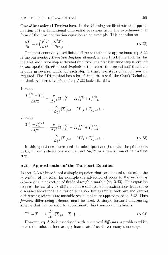
Two-dimensional Derivatives. In the following we illustrate the approx­imation of two-dimensional differential equations using the two-dimensional form of the heat conduction equation as an example. This equation is:

8T _ (82T 82T) 8t - '" 8x2 + 8y2 (A.22)

The most commonly used finite difference method to approximate eq. A.22 is the Alternating Direction Implicit Method, in short: ADI method. In this method, each time step is divided into two. The first half time step is explicit in one spatial direction and implicit in the other, the second half time step is done in reverse. Thus, for each step in time, two steps of calculation are required. The ADI method has a lot of similarities with the Crank Nicholson method. A discrete version of eq. A.22 looks like this:

1. step:

T+/2 - T-',) ',) - '" (T+/2 2T+/2 T+/2)

LJ.t/2 - LJ.x2 Hl,j - i,j + i-l,j

'" + LJ.y2 (TiJ+1 - 2TiJ + TiJ - 1 )

2. step:

T+ - T+/2 ',) ',) - '" (T+/2 2T+/2 T+/2)

LJ.t/2 - LJ.x2 Hl,j - i,j + i-l,j

'" ( + + +) + LJ.y2 Ti,)+1 - 2Ti,j + Ti,j-l (A.23)

In this equation we have used the subscripts i and j to label the grid points in the x- and y-directions and we used "+/2" as a description of half a time step.

A.2.4 Approximation of the Transport Equation

In sect. 3.3 we introduced a simple equation that can be used to describe the advection of material, for example the advection of rocks to the surface by erosion or the advection of fluids through a marble (eq. 3.43). This equation require the use of very different finite difference approximations from those discussed above for the diffusion equation. For example, backward and central differencing schemes are unstable when applied to approximate eq. 3.43. Thus forward differencing schemes must be used. A simple forward differencing scheme that can be used to approximate this transport equation is:

LJ.t T+ = T- + u- (T-+ 1 - T-)

LJ.x' , (A.24)

However, eq. A.24 is associated with numerical diffusion, a problem which makes the solution increasingly inaccurate if used over many time steps.

362 A . Mathematical Tools

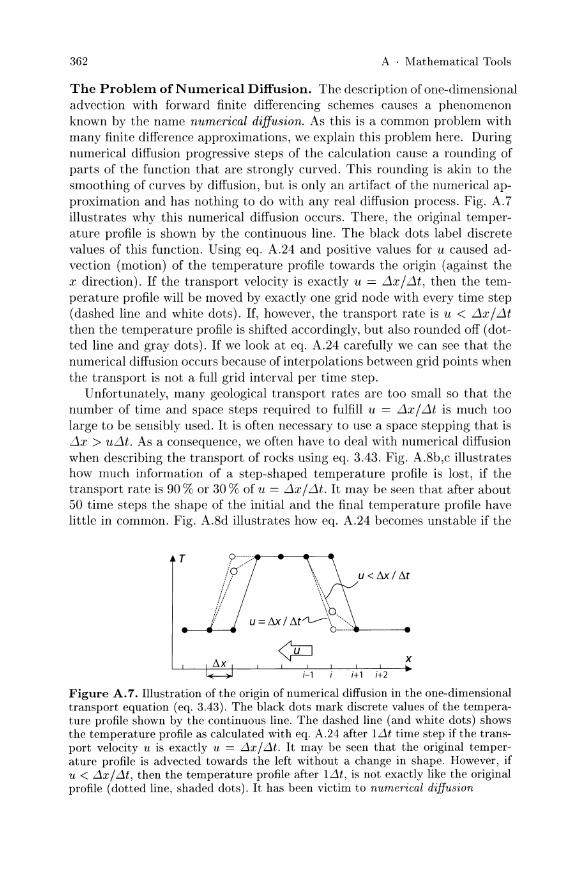
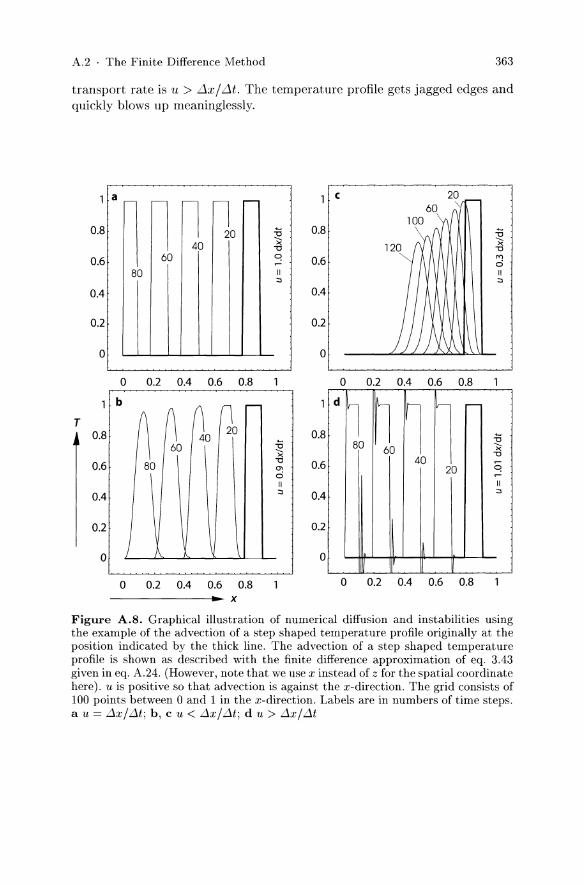
The Problem of Numerical Diffusion. The description of one-dimensional advection with forward finite differencing schemes causes a phenomenon known by the name numerical diffusion. As this is a common problem with many finite difference approximations, we explain this problem here. During numerical diffusion progressive steps of the calculation cause a rounding of parts of the function that are strongly curved. This rounding is akin to the smoothing of curves by diffusion, but is only an artifact of the numerical ap­proximation and has nothing to do with any real diffusion process. Fig. A.7 illustrates why this numerical diffusion occurs. There, the original temper­ature profile is shown by the continuous line. The black dots label discrete values of this function. Using eq. A.24 and positive values for u caused ad­vection (motion) of the temperature profile towards the origin (against the x direction). If the transport velocity is exactly u = iJ.x / iJ.t, then the tem­perature profile will be moved by exactly one grid node with every time step (dashed line and white dots). If, however, the transport rate is u < iJ.x / iJ.t then the temperature profile is shifted accordingly, but also rounded off (dot­ted line and gray dots). If we look at eq. A.24 carefully we can see that the numerical diffusion occurs because of interpolations between grid points when the transport is not a full grid interval per time step.

Unfortunately, many geological transport rates are too small so that the number of time and space steps required to fulfill u = iJ.x / iJ.t is much too large to be sensibly used. It is often necessary to use a space stepping that is iJ.x > uiJ.t. As a consequence, we often have to deal with numerical diffusion when describing the transport of rocks using eq. 3.43. Fig. A.8b,c illustrates how much information of a step-shaped temperature profile is lost, if the transport rate is 90 % or 30 % of u = iJ.x / iJ.t. It may be seen that after about 50 time steps the shape of the initial and the final temperature profile have little in common. Fig. A.8d illustrates how eq. A.24 becomes unstable if the

T u<I1xIM

I1x x ;-1 ;+1 ;+2

Figure A.7. Illustration of the origin of numerical diffusion in the one-dimensional transport equation (eq. 3.43). The black dots mark discrete values of the tempera­ture profile shown by the continuous line. The dashed line (and white dots) shows the temperature profile as calculated with eq. A.24 after L1t time step if the trans­port velocity u is exactly u = :1. x / :1.t. It may be seen that the original temper­ature profile is advected towards the left without a change in shape. However, if u < :1.x/:1.t, then the temperature profile after l:1.t, is not exactly like the original profile (dotted line, shaded dots). It has been victim to numerical diffusion

A.2 . The Finite Difference Method 363

transport rate is u > Llx / Llt. The temperature profile gets jagged edges and quickly blows up meaninglessly.

1 a - ,-- n ~o -0.8 -0 40 >< "0

1 c 20 60

100 0.8 -0

>< "0

0.6 60 q 0.6 ""' d 80 II II

'" '" 0.4 0.4

0.2 0.2

0 0

0 0.2 0.4 0.6 0.8 0 0.2 0.4 0.6 0.8

b

n. Qo .--

T n ~ 0.8 40 -0 ><

0.6 80 "0 0\

I d

d

l ~ Iii IIr- .--

-0 80 >< 40

"0

20 q ~

0.8

0.6

II II

0.4 '" 0.4 '"

0.2 0.2

0 / o I!

0 0.2 0.4 0.6 0.8 o 0.2 0.4 0.6 0.8 ~ x

Figure A.B. Graphical illustration of numerical diffusion and instabilities using the example of the advection of a step shaped temperature profile originally at the position indicated by the thick line. The advection of a step shaped temperature profile is shown as described with the finite difference approximation of eq. 3.43 given in eq. A.24. (However, note that we use x instead of z for the spatial coordinate here). u is positive so that advection is against the x-direction. The grid consists of 100 points between 0 and 1 in the x-direction. Labels are in numbers of time steps. au = f1x/f1t; b, c u < f1x/f1t; d u > f1x/f1t

364 A . Mathematical Tools

A.2.5 Dealing with Irregular Grid Boundaries

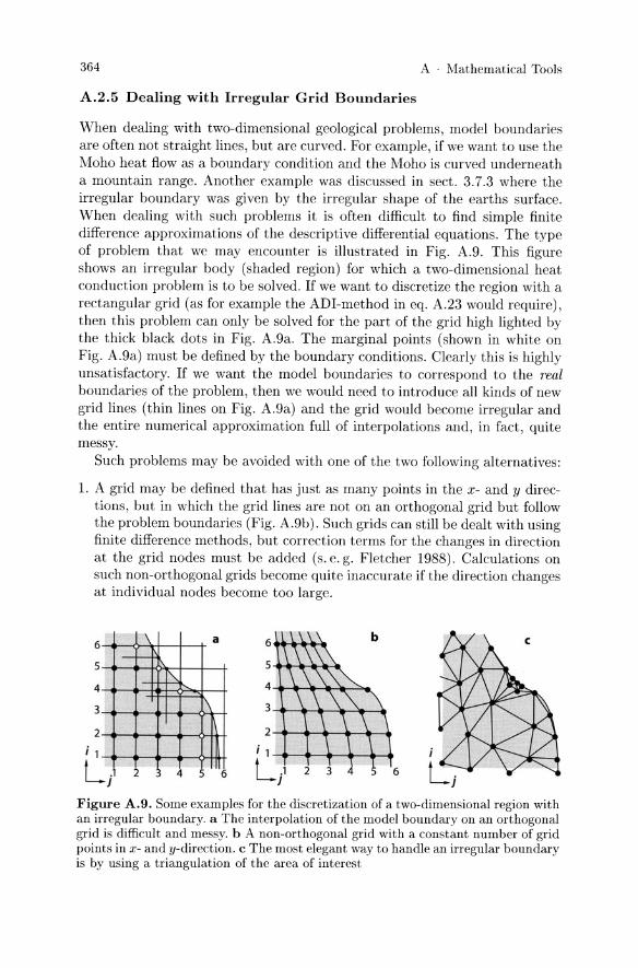
When dealing with two-dimensional geological problems, model boundaries are often not straight lines, but are curved. For example, if we want to use the Moho heat flow as a boundary condition and the Moho is curved underneath a mountain range. Another example was discussed in sect. 3.7.3 where the irregular boundary was given by the irregular shape of the earths surface. When dealing with such problems it is often difficult to find simple finite difference approximations of the descriptive differential equations. The type of problem that we may encounter is illustrated in Fig. A.9. This figure shows an irregular body (shaded region) for which a two-dimensional heat conduction problem is to be solved. If we want to discretize the region with a rectangular grid (as for example the ADI-method in eq. A.23 would require), then this problem can only be solved for the part of the grid high lighted by the thick black dots in Fig. A.9a. The marginal points (shown in white on Fig. A.9a) must be defined by the boundary conditions. Clearly this is highly unsatisfactory. If we want the model boundaries to correspond to the real boundaries of the problem, then we would need to introduce all kinds of new grid lines (thin lines on Fig. A.9a) and the grid would become irregular and the entire numerical approximation full of interpolations and, in fact, quite messy.

Such problems may be avoided with one of the two following alternatives:

1. A grid may be defined that has just as many points in the x- and y direc­tions, but in which the grid lines are not on an orthogonal grid but follow the problem boundaries (Fig. A.9b). Such grids can still be dealt with using finite difference methods, but correction terms for the changes in direction at the grid nodes must be added (s. e. g. Fletcher 1988). Calculations on such non-orthogonal grids become quite inaccurate if the direction changes at individual nodes become too large.

6

5

4

3

2

; 1

.1 LJ

-\

r--["-.,

\

4

a 6 b

5

4

3

2

II ; , n6 L/ 2

Figure A.9. Some examples for the discretization of a two-dimensional region with an irregular boundary. a The interpolation of the model boundary on an orthogonal grid is difficult and messy. b A non-orthogonal grid with a constant number of grid points in x- and y-direction. c The most elegant way to handle an irregular boundary is by using a triangulation of the area of interest

A.3 . Scalars, Vectors and Tensors 365

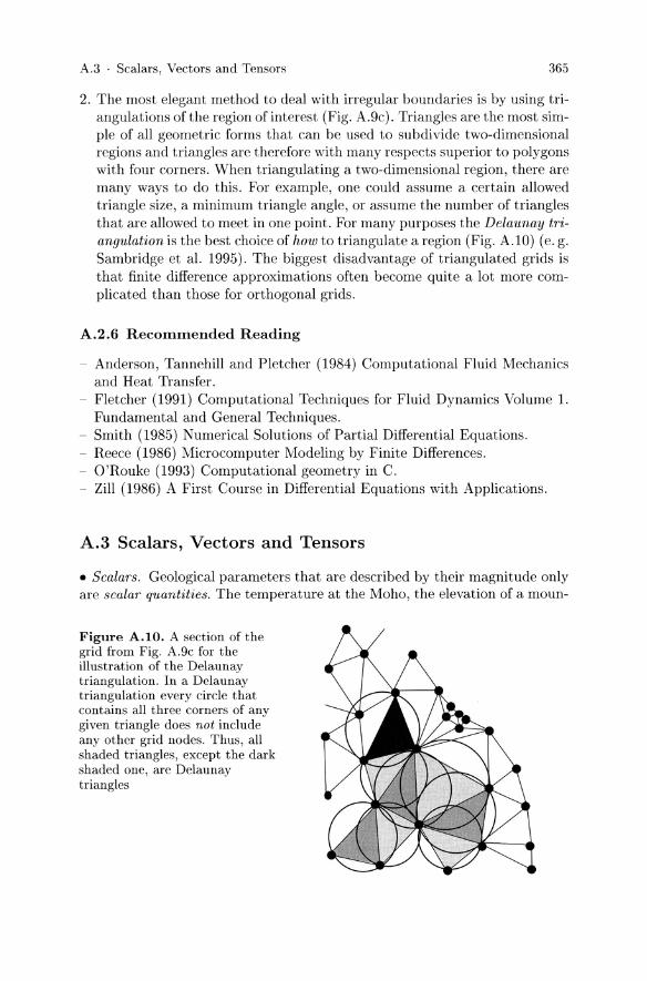
2. The most elegant method to deal with irregular boundaries is by using tri­angulations of the region of interest (Fig. A.9c). Triangles are the most sim­ple of all geometric forms that can be used to subdivide two-dimensional regions and triangles are therefore with many respects superior to polygons with four corners. When triangulating a two-dimensional region, there are many ways to do this. For example, one could assume a certain allowed triangle size, a minimum triangle angle, or assume the number of triangles that are allowed to meet in one point. For many purposes the Delaunay tri­angulation is the best choice of how to triangulate a region (Fig. A.10) (e. g. Sambridge et al. 1995). The biggest disadvantage of triangulated grids is that finite difference approximations often become quite a lot more com­plicated than those for orthogonal grids.

A.2.6 Recommended Reading

- Anderson, Tannehill and Pletcher (1984) Computational Fluid Mechanics and Heat Transfer.

- Fletcher (1991) Computational Techniques for Fluid Dynamics Volume l. Fundamental and General Techniques.

- Smith (1985) Numerical Solutions of Partial Differential Equations. - Reece (1986) Microcomputer Modeling by Finite Differences. - O'Rouke (1993) Computational geometry in C. - Zill (1986) A First Course in Differential Equations with Applications.

A.3 Scalars, Vectors and Tensors

• Scalars. Geological parameters that are described by their magnitude only are scalar quantities. The temperature at the Moho, the elevation of a moun-

Figure A.10. A section of the grid from Fig. A.9c for the illustration of the Delaunay triangulation. In a Delaunay triangulation every circle that contains all three corners of any given triangle does not include any other grid nodes. Thus, all shaded triangles, except the dark shaded one, are Delaunay triangles

366 A . Mathematical Tools

tain, density of a rock or pressure are examples. (According to Oertel 1996 pressure should be referred to as an isotropic tensor of second rank but for all intents and purposes of this book it is sufficient to treat it as a scalar). Variables that are scalar quantities are commonly denoted with italics, as most variables in this book.

• Vectors. Geological parameters that have both a magnitude and a direction are described by vectors. An example is the force with which India and Asia collide or the rate of intrusion of a magmatic body. The former is roughly 1013 N m- 1 and is directed northwards; the latter might be some meters per year and directed upwards in the crust. Vectors are commonly represented by bold roman letters, although we refrain from this use in this book.

• Tensors. Parameters that are characterized by not only their magnitude and their direction, but also by a spatial dependence of this direction are described by tensors (s. Twiss and Moores 1992; Oertel 1996). The state of stress at a point or strain rate are the most familiar examples of tensor quantities to a geologist. It is easy to see that magnitude and direction alone are insufficient to describe stress. For example, the tensor components a xx

and a yx both act in the x direction and they also may both be of the same magnitude. However, a xx is a normal stress and a xy is a shear stress, i.e. they are exerted onto planes of different orientation. Tensors are represented as matrices and are commonly abbreviated with italics. As for vectors, we do not use this notation in the present book as the tensorial quantities occurring herein (e.g. strain rate or stress) are usually simplified enough so that they reduce to simple scalar quantities (e.g by considering one-dimensional cases only).

Scalars, vectors and tensors are often called tensorial quantities of the 0., 1. and 2nd rank. In this book we treat many quantities that are actually described by vectors or tensors as if they were scalars (except in sect. 5.1.1). We have done so by making our problems so simple, so that they may be treated one-dimensionally. Only then we were able to treat many of these parameters as scalars. In fact, it is better to call them "pseudoscalars" because it is always implicit that their direction is known. Regardless, we introduce some of the basic principals of vector calculations on the following pages.

• Common confusions. Quantities described by scalars, vectors and tensors are often confused in the literature. Even in this book - while we try not to confuse them - we often treat tensorial quantities as if they were scalars. When doing so, we always need to remember that our considerations remain one-dimensional. For the correct consideration of two and three-dimensional problems, the full tensor quantities must be considered. Products and sums of tensors are not described by the sum of the one-dimensional descriptions in several spatial directions alone (e. g. Oertel 1996; Strang 1988) and it is therefore often not trivial to understand the results of two- and three­dimensional models in comparison to their one-dimensional equivalents.

A.3 . Scalars, Vectors and Tensors 367

• Vectors. Vectors describe direction and magnitude of a parameter. Thus, in Cartesian coordinates, they are described by three components:

(A.25)

U x , u y and U z are called the vector components of the vector u and i, j and k are called the unit vectors in the three orthogonal spatial directions. The unit vectors are often omitted and vectors are usually just written as a list of three scalar components. In the literature, these are variably named ux, uy, Uz or u, v, w or Ul, U2, U3' In the following we use the first of these three notation rules. Note that vectors are commonly represented with bold characters.

The sum of two vectors u and v is given by the sum of the vector compo­nents:

w = u + v = (ux + vx)i + (u y + vy)j + (u z + vz)k (A.26)

This sum is often written as:

w = (ux + vx , uy + vy, Uz + vz ) (A.27)

The magnitude (or length) of a vector is given by:

lui = Ju~ + u~ + u~ . (A.28)

Eqs A.25, A.26 and A.28 may be intuitively or graphically followed using the Pythagoras theorem.

The scalar- or dot product of two vectors is a scalar quantity which is defined as the sum of the products of two vector components:

u. v = UxVx + UyV y + UzVz . (A.29)

This is equivalent to the product of the magnitudes of the two vectors and the cos of the angle ¢ between them:

u. v = lullvl cos¢ . (A.30)

The scalar product has its name because the result is a scalar quantity. A nice example for a scalar product is the work required to move a plate with the force F (being a vector) for the distance 1 (having a length and a direction) .

The cross product or vector product is denoted with x or 1\. The result is a vector. It is defined as follows:

w = u x v = u 1\ v = (uyv z - uzvy, UzVx - UxVz, uxvy - uyvx) . (A.31)

The three values on the right hand side of eq. A.31 have the form of the determinants of matrices. Thus, vector products may be solved using the methods of matrix calculations which are not treated here. A good example for a vector product is the velocity vector. It is described by the product of the angular velocity vector wand the position vector r.

368 A . Mathematical Tools

• Grad, Div and Curl. The gradient of a scalar valued function (denoted with "Grad" or "Del" or: V; s. sect. 3.1.1) is a vector describing the spatial change of this function. It is defined as

(A.32)

Thus, the spatial change of temperature (as a function of x, y and z: T = T(x, y, z)), may be described as follows:

( 8T 8T 8T) Grad T == VT = 8x' 8y' 8z (A.33)

The vector "Grad T" is normal to surfaces of constant temperature just like the dip direction of a surface is always normal to the contour lines. "Grad" is a handy tool for the description of the topography of any potential surface.

The divergence of a vector is a scalar. In the earth sciences it often describes the transfer rate of mass or energy. The divergence of a vector is defined as follows:

DIV V = V • v = - + - + -. _ (8vx 8vy 8Vz) 8x 8y 8z

(A.34)

Let us illustrate the divergence of a vector valued function dependent on the spatial coordinates x, y and z with an example. Assume that v is the rate of mass or energy transfer. The flow of mass is qf = pv and the flow of energy is: q = Hv. There, p is density in kgm-3 and H is the volumetric energy content in Jm-3 . Thus, flow has the units ofkgm-2 s- I or Wm- 2 ,

respectively. The divergence of these flows is the sum of the change in flow in the three spatial directions (eq. A.34). If the flow of energy or mass into a unity cube is just as large as the flow out of it (general criterion for the conservation of mass), then Div v = 0 (s. also sect. 3.1.1,3.3).

The Curl or Rot of a vector field is a vector describing the rotation of a vector. A vector with Curl u = 0 is called non rotating. The Curl is defined by the relationship:

Curl v == Rot v == V x v

_ (8Vz 8vy 8vx 8vz 8vy 8Vx )

- 8y - 8z ' 8z - 8x' 8x - 8y (A.35)

AA An Example for Using Fourier Series

In sections 3.1.1, 3.6.1 and 3.4.1 we have been introduced to two different types of solutions of the diffusion equation (eq. 3.6). They are:

A.4 . Fourier Series 369

1. Solutions that may be found by integration. These include mainly problems for which the descriptive equations may be so much simplified so that it is straight forward to integrate them. Very often, these are steady state problems in which it is possible to assume dT jdt = o.

2. Solutions containing an error function. These may be found for problems that have their boundary condition at infinity. For example, when describ­ing the thermal evolution of intrusions that are much smaller than the thickness of the crust or their distance to the earths surface, it is possible to make this assumption (e.g. p. 102 or p. 174).

A third type of solution is necessary for time dependent problems with spa­tially fixed boundary conditions. We have encountered such examples when describing the erosion of mature landscapes between incising drainages with the diffusion equation, for example on p. 175. Such examples may be solved using Fourier series. As the diffusion equation is such a classic example where Fourier series find an important application, we will continue to use this equa­tion as an example. The now well familiar equation that we want to use again (eq. 3.6) is:

8T 82T at = K, 8x2 ' (A.36)

with T being a function of both space x and time t: T = T(x, t). Let us assume that this equation is subject to zero temperature boundary conditions at x = 0 and x = l which may be formulated as:

T = 0 at x = 0 at time t > O. T = 0 at x = l at time t 2': O.

With these boundary conditions, this problem corresponds to that dis­cussed on page 175. There, D and H correspond to what is here K, and T and the spatial extent of the problem was there measured between -l and l, while it is here only from 0 to l. On page 175 we just gave the solution of this problem in eq. 4.63 without detailing the methods of solution.

In order to understand the process of solution here in some more detail, consider the following: Eq. A.36 is satisfied if we find a term for which the first time derivative is directly proportional to the second spatial derivative. The proportionality constant is K,. A general function that satisfies this condition and the boundary conditions has the form:

(A.37)

There, an and bn are constants. Let us discuss why this solution satisfies eq. A.36 and how it may be derived:

370 A . Mathematical Tools

1. We can see that the solution above contains an exponential function of time and a sine-function of x. This can be understood as follows: Differen­tiating an exponential function will always return an exponential function. Correspondingly, the second derivation of a sine-function is a negative sine function. This negative will result in the exponential function also being negative (as shown below), which gives a function that decays with time. Thus, the first derivative of eq. A.37 with respect to t, will always be pro­portional to its second derivative with respect to x. Thus, the condition of the diffusion equation is met, if the correct constants are found.

2. It may be seen that the boundary conditions at x = 0 and x = Z are always satisfied as the sine-function is always zero at these two values of x. Thus, temperature there is also always zero.

3. The fact that the solution contains an infinite sum is a generalization. If a single term of the infinite sum satisfies eq. A.36, so will the infinite sum of a series of terms.

Let us check if eq. A.37 actually satisfies eq. A.36. For clarity, we perform this check only for a single term of the infinite sum. For our check we differ­entiate this term with respect to time as well as space. The time derivative gives:

aT b bt· (n7rx) - =a e sm --at Z

The spatial derivatives are:

aT = n7ra ebtcos (n7rx) ax Z Z

as well as:

a2T n27r2a bt. (n7rx) ax2 = - -Z-2-e sm -Z-

(A.38)

(A.39)

(A.40)

Comparing eq. A.38 and eq. A.40 shows that eq. A.36 is satisfied if the constant b has the following value:

(A.41)

If we insert b from eq. A.41 in eq. A.37, we have an equation that satisfies all conditions of eq. A.36. The values for the constants an can be determined from the initial conditions. At time t = 0, ebt = 1 and thus from eq. A.37 it is true that:

00

T(x, 0) = f(x) = L ansin (n;x) n=O

(A.42)

Eq. A.42 is an example of a Fourier senes. The coefficients an can be determined from the integral:

A.4 . Fourier Series 371

2 rl . (n7rx) an = I 10 f(x)sm -1- dx , (A.43)

the derivation of which does not follow directly from eq. A.42 and will not be discussed here. However, it may be found in any book on Fourier series. The coefficients may be evaluated from this integral if the initial condition T(x,O) = f(x) is known. However, this integral is only easily evaluated for certain functions of f(x). For more general functions, solutions to this integral may be obtained from either math tables or numerically.

T

2

o

o 2 4 6 8 x

T

2

o L 9 terms

b

o 2 4 6 8 x

Figure A.ll. a The function I(x) = 2 (thick line) and the first five terms of an infinite sum of sine functions from eq. A.42 at time t = O. b The sum of the first two, three and nine terms of the function shown in a. It may be seen that the sum of only few terms is sufficient to approximate the thick drawn function in a quite good

• Solving eq. A.36 for non-zero boundary conditions. We can take this ap­proach one step further to solve the diffusion equation eq. A.36 for non-zero boundary conditions:

T = Tl at x = 0 at time t 2: O. - T = T2 at x = 1 at time t 2: o.

and initial conditions T = f(x) at t = O. In this case, the temperature T should evolve with time to the steady-state solution that satisfies the bound­ary conditions. We will denote the steady-state solution as g(x). It can be shown that g(x) = Tl + (T2 - Tdx/l. The solution for T has the form:

00

T = g(x) + L anebntsin (n7x) n=O

(A.44)

where bn is given by equation eq. A.41 and an has the form

an = ~ 11 (f(x) - g(x)) sin (n7x) dx . (A.45)

372 A . i\Iathematical Tools

A.5 Selected Numerical Tricks

A.5.1 Integrating Differential Equations

For many differential equations there are mathematical reference books con­taining their solutions and it certainly goes beyond the scope of this book to go into details of complicated integration methods. However, one simple example which illustrates the type of thinking that lies behind integrations like the one we used in sect. 4.1.2 will be introduced here. Eq. 4.9 has the form

dy -1 = ay + b , ( :c

(A.46)

where a and b are constants. The equation states that the differential of the variable y is proportional to y. This information is sufficient to be able to guess that the solution will contain an exponential function of the form eX, because exponential functions always remain exponential functions when they are differentiated (s. Table B.2). Thus, we may guess that the solution ,vill have the form:

y = qr,(rx) + d

and thus:

dy = qce(c,l') dx

(A.47)

(A.48)

Inserting eq. A.47 and eq. A.48 in eq. A.46 shows that c = (L and d = -b/a. It follows that:

b y = qe (ax) _ _ , (A.49) a

for a fixed scalar q.

A.5.2 Analytically Unsolvable Equations

Many equations cannot be solved analytically. However, they often may be evaluated numerically by separating them into two parts. We illustrate this using the transcendental eq. 6.3 as an example. This equation has the form

r::1: = ae - bx + d . (A.50)

All other parameters that occur in eq. 6.3 are summarized in eq. A.50 into the constants (L, b, c and d. Eq. A.50 cannot be solved for x. In order to solve it numerically it is useful to split the right hand side and the left hand side of the equation into two new equations. For the left side we ,vrite:

z = cx (A.51)

A.5 . Selected Numerical Tricks 373

and for the right side we write:

In (z-d) x= a

-b z=ae-bx+d or: (A.52)

These two functions are plotted in Fig. A.12. With the constants a = 1, b = 2, c = 3 and d = 3, the steep linear curve is eq. A.51 and the curve with a negative slope is eq. A.52. Their intersection is the solution of eq. A.50. This point may be found by alternating solution of eq. A.51 and A.52. For this we guess a value for x, insert this into eq. A.51 to calculate z and then insert this value for z into eq. A.52 to obtain a new x. For the example illustrated in Fig. A.24 an initial guess of x = 0 leads to the series: z = 4, x = 1.333, z = 3.069, x = 1.023, z = 3.129, x = 1.043, z = 3.124 and so forth. The result converges to a solution of approximately x ::::;j 1.04 and z ::::;j 3.12. The exact solution may be approximated as closely as desired. While the method is very simple, it may also lead to wrong results, for example if one of the two functions has local minima or maxima.

A.5.3 The Least Squares Method

A common problem in science occurs when a curve should be fitted to a num­ber of data points and the fit of the data to this curve should be quantified. The most common method for this is to find the smallest sum of the squares of the deviations of the data from the curve, in short, the least squares. In the following section we explain how this is done with the example of a linear fit, i.e. the curve that is fitted to the data is a straight line. However, for more complicated choices of functions, the same rules apply. We assume that the data consist of n values for y and just as many for x. We label the data with Yi and Xi from i = 1 to n. The straight line we will to fit through the data cloud has the form y = ax + b where a and b are unknown. If we insert our data pair for x and y into this linear equation, we obtain:

Figure A.12. Illustration of the numerical solution of eq. A.50. The constants are a = 1, b = 2, c = 3 and d = 3. The straight line respresents eq. A.51, the curved line is eq. A.52. The dashed line shows the iterative approximation of their intersection

z

4

3

o x

374 A . Mathematical Tools

Yi = aXi + b - e , (A. 53)

where e is the deviation of a given data point from the fitted line. In order to minimize the sum of the squares of this deviation, the sum of all e must be minimized. This means that:

n n

(A.54)

must be minimized. In order to do so, eq. A.54 may be partially differentiated with respect to a and b, set to zero and solved for a or b. Using the simple differentiation rules from Table B.1 the derivative with respect to a may be found to be:

(A.55)

The derivative with respect to b is:

0= 8 (L~=l (axi + b - YY) = ~ 2(axi + b _ Yi)2 8b ~

i=l (A. 56)

Eqs. A.55 and A.56 may be simplified and solved simultaneously for a and b. We get:

n (L~=l XiYi) - (L~=l Xi) (L~=l Yi) a = --.:.::="'-( ",----'-n --'.....-2-') =(=",-n-'-'=):":::2 =..0....:.."':" ,

n L....i=l Xi - L....i=l Xi (A.57)

b = (L~=l Yi) (L:~l x7) - (L~=l Xi) (L;~l XiYi)

n (~~=l xT) - (~;~l xd 2 (A.58)

These are the coefficients of the best fitting straight line of eq. A.53. These two equations (eq. A.57 and eq. A.58) are straight forward to implement on a computer.

A.5 . Selected Numerical Tricks 375

The errors of these values, as given by their standard deviations are simply given by:

(A.59)

and:

(A.50)

A.5.4 Basic Statistical Parameters

A fundamental task of geologists is the characterization of the location and the variability of a data set, for example P-T data determined with ther­mobarometry, geochronological data, numbers from a whole rock analysis, digital data during image processing or dip and strike data measured in the field. Because such measurements may be very precise, but they are never perfectly accurate it is necessary to evaluate them statistically (s. p. 5). The most important parameters for such an evaluation are summarized here .

• Normal distribution. The statistical interpretation of many geological data is based on the assumption that the data have a normal (also called Gaussian) distribution around the exact value. A distribution is said to be normal if its probability density function is given by:

_ ( 1 ) (-('2-';/) f(x) - r.>= e .

(Jy27r (A.51)

This function is characterized by two parameters called the mean, fl, and the standard deviation (J. Eq. A.51 is plotted in Fig. A.13 and may be in­terpreted as the enveloping curve of a histogram. If the data are centered around a mean of fl = 0 and the standard deviation is (J = 1, then eq. A.51 simplifies to: f(x) = e-(x2 /2) /V2ir. The distribution is said to be a standard normal distribution .

• Mean. The mean of a data set indicates the most probable location of the exact value. For a data set S containing n data Si it is defined as:

(A.52)

the mean gives themost probable location of the exact value.

376

f(x) a normal distribution

A . Mathematical Tools

b

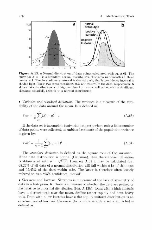
Figure A.13. a Normal distribution of data points calculated with eq. A.61. The curve for a = 1 is a standard normal distribution. The area underneath all three curves is 1. The 1a confidence interval is shaded dark, the 2a confidence interval is shaded light. These two areas contain 68.26% and 95.45% ofthe data, respectively. b shows data distributions with high and low kurtosis as well as one with a significant skewness (shaded), relative to a normal distribution

• Variance and standard deviation. The variance is a measure of the vari­ability of the data around the mean. It is defined as

1 n .) Var = - 2)Si - f.1)~ .

n (A.63)

i=l

If the data set is incomplete (univariat data set), where only a finite number of data points were collected , an unbiased estimate of the population variance is given by:

lIn .J

Var = -- '"(Si - f.1)~ n-1L..-

';=1

(A.64)

The standard deviation is defined as the square root of the variance. If the data distribution is normal (Gaussian), then the standard deviation is abbreviated with a = ,tVar. From eq. A.61 it may be calculated that 68.26% of all data of a normal distribution will fall within ±la of the mean and 95.45% of the data within ±2(J. The latter is therefore often loosely referred to as a "95% confidence interval" .

• Skewness and kurtosis . Skewness is a measure of the lack of symmetry of data in a histogram. Kurtosis is a measure of whether the data are peaked or flat relative to a normal distribution (Fig. A.13b). Data with a high kurtosis have a distinct peak near the mean, decline rather rapidly and have heavy tails. Data with a low kurtosis have a flat top. A uniform distribution is an extreme case of kurtosis. Skewness (for a univariate data set s. eq. A.64) is defined as:

A.6 . Problems 377

1 ~ 3 skew = (J3(n _ 1) L)5i - /1)

1=1

(A.65)

Kurtosis is defined as:

(A.66)

Many classical statistical tests depend on the assumption that the data have a normal distribution. Significant skewness and kurtosis indicate that the data are not normal. In fission track analysis the skewness and kurtosis of track length distributions bear significant information on the cooling history of the rocks.

A.6 Problems

Problem A.1. Fin'ite difference approximations (p. 855): Eq. 3.45 describes simultaneous diffusion and one-climensional mass trans­port. \Vrite an explicit finite difference approximation for this equation. Use a forward differencing scheme to approximate the transport term. Follow the schemes introduced in eq. A.14 and eq. A.15

Problem A.2. Finite difference approx'imations (p. 856): Eq. 4.46 describes the clastic bending of oceanic lithosphere under applied loads. There, w is the variable for which we want to solve the equation. It is the vertical deflection of the bent plate as a function of distance x. Write an explicit finite differmce approximation for this equation. Hint: it is easiest to just expand the scheme we have followed in cq. A.16

Problem A.3. Finite differ'ence approximations (p. 862): Redraw Fig. A.7 carefully to convince yourself why backward finite differenc­ing schemes will be unstable when describing the transport equation. For your considerations look at the scheme of eq. A.24, and a corresponding backward differencing scheme for tl = LJ.x / LJ.t.

Problem AA. Mean and standard deviation (p. 862): Determine the mean and the standard deviation of the following two data sets 51 = {10, 10, 10, 10,6,6,6, 6} and 52 = {I, 5, 10,20, 15,9,4, O}, assuming that both data sets are samples from a normal distibutioll.

B. Maths Refresher

Recommended Reading:

- Abramowitz and Stegun (1972) Handbook of Mathematical Functions. - Press, Flannery, Teukolsky and Vetterling (1989) Numerical Recipes. - Strang (1988) Linear Algebra and Applications.

Table B.I. General rules of differential calculus using the example of the function y = f(x). u and v are also functions of x. a is a constant. f'(x) or y' is the first derivative of y with respect to x

f(x)

y = au

y = x a

y = aX

y = XX

y=u+v

y = uv

y=;

y = U V

j'(x)

y' = a(du/dx)

y' = axa - 1

y' = aXln(a)

y' = (1 + In(x»x X

y' = (du/dx) + (dv/dx)

y' = u(dv/dx) + v(du/dx)

y' = (vdu/dx - udv/dx)/v 2

y' = U V ((v/u)(du/dx) + lnu(dv/dx»

380

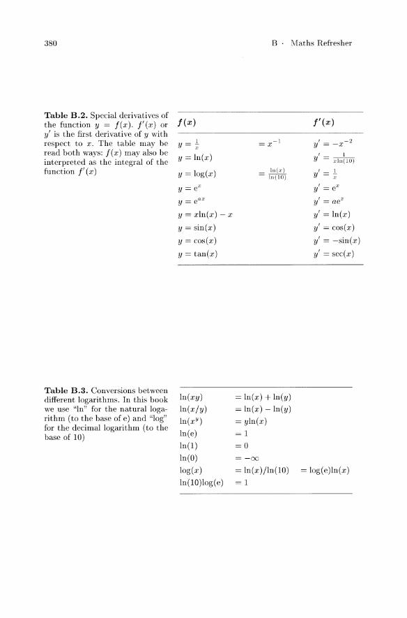
Table B.2. Special derivatives of the function y = f(x). f' (x) or y' is the first derivative of y with respect to x. The table may be read both ways: f(x) may also be interpreted as the integral of the function f' (x)

Table B.3. Conversions between different logarithms. In this book we use "In" for the natural loga­rithm (to the base of e) and "log" for the decimal logarithm (to the base of 10)

f(x)

y=~ y = In(x)

y=log(x)

y=xln(x)-x

y=sin(x)

y = cos(x)

y = tan(x)

In(xy)

In(x/y)

In(xY)

In(e)

In(l)

In(O)

log(x)

In(10)log( e)

B· Maths Refresher

-1 =x

_ In(x) - In(10)

= In(x) + In(y)

= In(x) -In(y)

=yln(x)

=1

=0 =-00

f'(x)

y' = _x- 2

, 1 Y = xln(10)

y' = ~ y' = eX

y' = aex

y'=ln(x)

y' = cos (x)

y' = -sin(x)

y' = sec(x)

= In(x)/ln(10) = log(e)ln(x)

=1

B· Maths Refresher

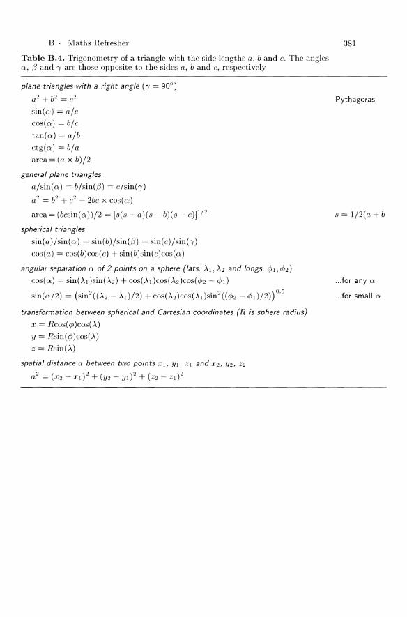
Table B.4. Trigonometry of a triangle with the side lengths a, band e. The angles 0:, (3 and '"Y are those opposite to the sides a, band e, respectively

plane triangles with a right angle ('"'( = 900 )

a2 + b2 = e2

sin(o:) = a/e

cos(o:) = b/e

tan(o:) = alb

ctg(o:) = b/a

area = (a x b)/2

general plane triangles

a/sin(o:) = b/sin((3) = e/sin('"'()

a2 = b2 + e2 - 2be x cos(o:)

area = (besin(0:))/2 = [8(8 - a)(s - b)(8 - e)p/2

spherical triangles

sin(a)/sin(o:) = sin(b)/sin((3) = sin(c)/sin('"'()

cos( a) = cos(b )cos( c) + sin(b )sin( e )cos( 0:)

angular separation 0: of 2 points on a sphere (fats. )\1, A2 and longs. (/JI, rjJ2)

cos(o:) = sin(Al)sin(A2) + cos(AdcoS(A2)COS(rjJ2 - rjJl)

sin(0:/2) = (sin2 ((A2 - Al)/2) + COS(A2)COs(Adsin2((rjJ2 - rjJl)/2))O.5

transformation between spherical and Cartesian coordinates (R is sphere radius)

x = Rcos(rjJ)COS(A)

y = Rsin(rjJ)cos(A)

z = Rsin(A)

spatial distance a between two points Xl, Yl, Zl and X2, Y2, Z2

a2 = (X2 - Xl? + (Y2 - yd 2 + (Z2 - zd 2

381

Pythagoras

8=1/2(a+b

... for any 0:

... for small 0:

382 B· Maths Refresher

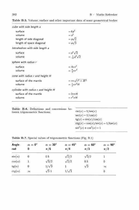
Table B.5. Volume, surface and other important data of some geometrical bodies

cube with side length a

surface

volume

length of side diagonal

length of space diagonal

tetrahedron with side length a

surface

volume

sphere with radius r

su rface

volume

cone with radius r and height H

surface of the mantle

volume

cylinder with radius r and height H

surface of the mantle

volume

=6a2

=a3

=aV2 =aV3

=a2 V3 = -&.iV2

= r7rv'r2 + H2 = ~7fr2H

Table B.6. Definitions and conversIOns be­tween trigonometric functions csc(x) = l/sin(x)

sec(x) = l/cos(x)

tg(x) = sin(x) /cos(x)

ctg(x) = cos(x)/sin(x) = l/tan(x)

sin2 (x) + cos2 (x) = 1

Table B.7. Special values of trigonometric functions (Fig. B.1)

Angle Q = 0° Q = 30° Q = 45° Q = 60° Q = 90° rad 0 7r /6 7r /4 7r /3 7r /2

sin (a) 0 0.5 V2/2 V3/2 1 cos (a) 1 V3/2 V2/2 0.5 0

tg(oo) 0 1/V3 1 V3 00

ctg(oo) 00 V31 1/V3 0

B· Maths Refresher

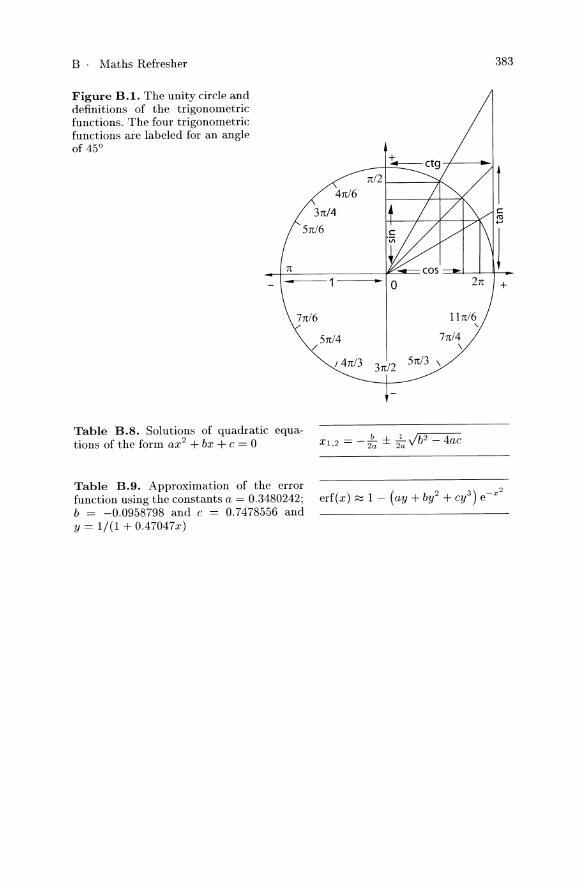
Figure B.1. The unity circle and definitions of the trigonometric functions. The four trigonometric functions are labeled for an angle of 45°

411:/6

311:/4

511:/6

11:/2 /-__ """*,-

711:/6

511:/4 /

711:/4 \

I 411:/3 311:/2 511:/3 \

Table B.S. Solutions of quadratic equa-tions of the form ax2 + bx + c = 0 X),2 = - 2: ± t;Jb2 - 4ac

383

+

Table B.9. Approximation of the error function using the constants a = 0.3480242; erf(x) ~ 1 - (ay + by2 + cy3) e- x2

b = -0.0958798 and c = 0.7478556 and y = 1/(1 + O.47047x)

c. Symbols and Units

386 C . Symbols and Units

Table C.l. Symbols and units of the variables used in this book. Physical constants of the earth are listed in Table C.3 and C.4. Variables abbreviated with Greek letters are explained in Table C.2. Variables used in the text are often specified in more detail by adding a subscript. For example q is used for heat flow, and qs for surface heat flow. The most commonly used subscripts in this book are l for lithosphere; c for crust; m for mantle; i, j and n for numbering; x, y and z for spatial directions and 0 for initial values

Symbol Variable Unit 1. Occurrence

Ar Argand number Eq.6.27 A area m2 Eq.3.2

A pre exponential constant MPa- ns- 1 Eq. 5.38

Aq · .. of quartz creep MPa- n S-l Table 5.3

Ao · .. of olivine creep MPa- n S-l Table 5.3 a general constant variable Eq. 3.20 b general constant variable Eq. 3.20

cp heat ca pacity (of rocks) ::::: 1000 J kg- 1 K- 1 Eq.3.4

Cpf · .. of fluids J kg- 1 K- 1 Eq. 3.50 C constant of integration variable Eq. 3.58 D angular momentum kg m2 S-l Sect. 2.2.4 D rigidity of elastic plates Nm Eq.4.41 D deformation Sect. 7

D diffusivity of mass m2 S-l Eq.4.54

Do pre exponential diffusivity m2 S-l Eq.7.4 e elongation Eq.5.1 e error Eq. A.53 E Young's Modul Pa Eq.4.43 E energy J

Ep potential energy (per area) J m- 2 Eq. 5.44 Ek kinetic energy J Eq. 5.58

f frequency S-l Eq. 3.103 f ellipsidity Eq.4.1 fc vertica I stra i n of crust Eq.4.3 ~ vertical strain of lithosphere Eq.4.3 F force N Sect. 2.2.4

Fb buoyancy force (per length) N m- 1 Eq. 5.44

Fd tectonic driving force (per length) N m- 1 Eq.6.22

Feff effective driving force (per length) N m- 1 Eq.6.22

~ integrated strength N m- 1 Eq. 5.43

g geothermal gradient °Cm- 1 Eq. 3.48

g acceleration (gravitational) ms-2 Eq.4.16

C . Symbols and Units 387

Table C.l. ... continuation

Symbol Variable Unit 1. Occurrence

G geometrical factor for Tc Eq.7.9 G Gibb's energy J Eq.7.5 h elastic thickness m Eq. 4.43 h dimensionless height Eq. 1.2 h, exponential drop off m Eq. 3.67 hs erodable thickness m Eq. 4.55

H heat content (vol u metric) J m- 3 Fig. 3.10; Eq. 3.99 H elevation, height m Eq. 1.2

momentum kg m S-1 Sect. 2.2.4 tensor invariant Eq.5.5

J moment of inertia kgm 2 Sect. 2.2.4

k thermal conductivity J S-1 m- 1 K- 1 Eq.3.1 K bulk modulus Pa Sect. 5.1.2 K equilibrium coefficient Eq.7.5 I thickness, length scale m Eq. 3.18

L latent heat of fusion J kg- 1 Eq. 3.34 L sediment thickness m Eq.6.2

La · .. of decompacted layer m Eq.6.2 L* · .. of decompacted pile m Eq.6.2

m mass kg Eq. 1.1 M bending moment N Eq. 4.41 N number, counter Eq. 3.93 n power law-exponent Eq. 5.39 n general counter Eq. 3.16 Pe Peclet number Eq. 3.51 P pressure Pa Eq.5.7 Q activation energy (diffusion) J mol- 1 Eq. 7.4 Q activation energy (creep) J mol- 1 Eq. 5.38

Qq · .. of quartz creep J mol- 1 Table 5.3

Qo · .. of olivine creep J mol- 1 Table 5.3

QD · .. of Dorn law creep J mol- 1 Eq. 5.42 q load on a plate Pa Eq. 4.42

q heat flow Wm- 2 Eq. 3.1

qs · .. at the surface Wm- 2 Eq. 3.61

qm ... at the Moho Wm- 2 Eq. 3.61

q,ad · .. caused by radioactivity Wm- 2 Eq.6.13

q, water flux ms- 1 Eq. 4.71

qf sediment flux in rivers ms- 1 Eq. 4.71 r radius m Eq. 1.1, 3.12 r distance in polar coordinates m Eq. 1.1, 3.12 R radius of earth m Eq.2.1

RA · .. at the eq uator 6378.139 km Eq.4.1 Rp · .. at the pole 6356.75 km Eq.4.1

388 C . Symbols and Units

Table C.l. continuation

Symbol Variable Unit 1. Occurrence

5 stretch Eq.5.1

5 cooling rate DC S-l Eq. 3.90

5 rate of heat production J S-l m-3 Eq. 3.24

5chem ... chemical J S-l m- 3 Eq. 3.23

5mec · .. mechanical J S-l m- 3 Eq. 3.23

5rad · .. radioactive J S-l m- 3 Eq. 3.23

50 · .. radioactive at surface J S-l m-3 Eq. 3.67

5 entropy J K- 1 Eq.3.33 5L sea level m Eq.6.5 t time s Eq.3.4

ta degradation coefficient m2 Eq. 4.66 tE erosional time constant s Eq. 4.10 T temperature DC; K Eq.3.1

TA · .. at the start DC; K Eq.7.8 Tb · .. of the host rock DC; K Eq.3.85 Tc · .. closu re tem peratu re DC; K Eq.7.9 h · .. at the end DC; K Eq.7.8 T; · .. intrusion temperature DC; K Eq.3.85 Ii · .. at base of lithosphere ~ 1200-1300 DC Eq.3.60 Ii ... liquidus DC; K Eq. 3.41 Ts ... solidus DC; K Eq.3.41 Ts · .. at the su rface DC; K Eq.3.81 To · .. in itia Item peratu re DC; K Eq. 3.103

u velocity (often: in x direction) m S-l Eq. 3.43 U ci rcu mference m Sect. 4.0.1 v velocity (often: in y direction) m S-l Eq.4.4

Vf · .. of fluids m S-l Eq. 3.50

Vex exhumation rate m S-l Eq.4.4

Ver erosion rate m S-l Eq.4.7 Vro uplift rate of rocks m S-l Eq.4.4

Vup uplift rate of the surface m S-l Eq.4.4 V volume m3 Eq.3.2

w angular velocity S-l Sect. 2.2.4 w water depth m Eq.4.30 w plate deflection m Eq. 4.41 x spatial coordinate (horizontal) m Sect. 1.2 X mole fraction Eq.7.6

Y spatial coordinate (horizontal) m Sect. 1.2 Z spatial coordinate (vertical) m Sect. 1.2

Zc thickness of crust m Sect. 2.4.1; Eq. 3.63 z, initial depth m Eq.3.49 ZI thickness of lithosphere m Sect. 2.4.1 Zrad thickness of radioactive crust ~7-10 km Eq.3.61

c . Symbols and "Cnits 389

Table C.2. Greek symbols

Symbol Variable Unit 1. Occurrence

a coefficient of therma I expa nsion ::::; 3 . 10-5 °(-1 Eq. 3.32 a general angle radian Eq. 3.101 a flexural parameter m Eq. 4.47

f'3 isothermal compressibility Pa- 1 Eq. 3.31; 5.24 (-J stretching factor (mantle lithosph.) Eq. 6.10 8 stretching factor (crust) Eq. 6.10 8 density ratio Eq. 4.25 1/ viscosity Pa s Eq. 5.37 E strain Eq. 5.20

E strain rate S-l Eq. 1.5

'" diffusivity m2 S-l Eq.3.6 A longitude degree Eq. 2.2; Fig. 2.7 A wave length m Eq. 3.105 A pore fl u id pressu re ratio Eq. 5.29

Ac · .. in the crust Fig. 5.17 Al · .. in the lithosphere Fig. 5.17

J1. coefficient of internal friction Eq. 5.25 v Poisson ratio Eq. 4.43 ¢ latitude degree Fig. 2.7 ¢ porosity Eq. 3.50

¢o · .. at the su rface Eq. 6.1 dJ friction angle radian Eq. 5.28

P density kg m- 3 Eq.3.4

pc · .. of the crust kgm- 3 Eq. 4.18

pg · .. of sediment grains kg m- 3 Fig. 6.3; Eq. 6.7

po · .. of the mantle at OO( ::::; 3300 kgm- 3 Eq. 4.22

{JL · .. of a sedimentary pile kg m- 3 Eq.6.5

pm · .. of the mantle at ~ ::::; 3200 kg m- 3 Eq.4.18

pw · .. of water ::::; 1000 kgm- 3 Eq. 4.30 (7 stress Pa Eq.5.2

(71, (72, (73 principal stress Pa Eq.5.4 (7d differential stress Pa Eq. 3.25 (7n norma I stress Pa Eq. 5.25 (70 · .. critical, Dorn law creep Pa Eq. 5.42

T thermal time constant s Eq. 3.18 T shear stress Pa Eq.5.3 () dimensionless temperature Eq. 1.3; 3.88 () angle of a failure surface to (71 radian Fig. 5.6

e expa nsion ratio Eq. 4.25

390

Table C.3. Important data of the earth

equatorial radius

polar radius

diameter of core

volume

mass

surface area

area of the continents

area of continental lithosphere

area of oceanic lithosphere

mean elevation of the continents

mean depth of the oceans

total length of mid oceanic ridges

mean continental surface heat flow

mean oceanic surface heat flow

Table CA. Important physical constants

Constant

gas constant

gravitational constant

speed of light

Symbol

R

G

c

C . Symbols and Units

6378.139 km

6356.750 km

3468 km

1.083 . 1021 m3

5.973.1024 kg

5.10.1014 m2

1.48 . 1014 m2

2.0.1014 m2

3.1.1014 m2

825 m

3770m

~ 60000 km

~ 0.056 W m- 2

~ 0.078 W m- 2

Value

8.3144 J mol- 1 K- 1

6.6732.10-11 N m2 kg- 2

2.99792.108 m S-l

C . Symbols and Units 391

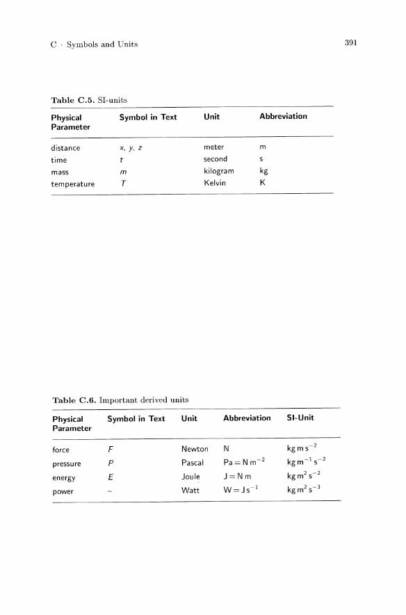
Table C.5. SI-units

Physical Symbol in Text Unit Abbreviation Parameter

distance x, y, z meter m

time second s

mass m kilogram kg

tem peratu re T Kelvin K

Table C.6. Important derived units

Physical Symbol in Text Unit Abbreviation 51-Unit Parameter

force F Newton N kg m S-2

pressure P Pascal Pa=Nm-2 kgm- 1 5- 2

energy E Joule J=Nm kg m2 5- 2

power Watt W = J 5- 1 kg m2 5-3

392 C . Symbols and Units

Table C.7. Conversions between derived units

Physical Parameter

force

pressure

energy

power

velocity

acceleration

Conversion

= mass x acceleration = pressure x distance = Pa m

=force per area = N m-2

= energy per vol u me = J m-3

= force x distance= Nm = mass x velocity2 = kg m2 S-2

= work per time = J S-l = W

= distance per time= m- 1

= velocity change per time = m s -2

C . Symbols and Units 393

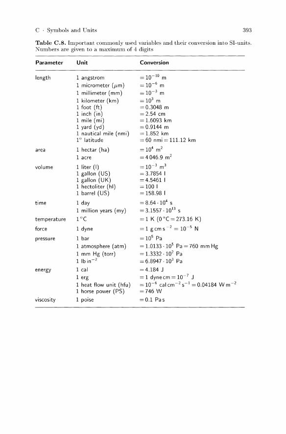
Table C.S. Important commonly used variables and their conversion into SI-units. Numbers are given to a maximum of 4 digits

Parameter

length

area

volume

time

temperature

force

pressure

energy

viscosity

Unit

1 angstrom

1 micrometer (pm)

1 millimeter (mm)

1 kilometer (km) 1 foot (ft) 1 inch (in) 1 mile (mi) 1 yard (yd) 1 nautical mile (nmi) 1 ° latitude

1 hectar (ha)

1 acre

1 liter (I) 1 gallon (US) 1 gallon (UK) 1 hectoliter (hi) 1 barrel (US)

1 day

1 million years (my)

1°C

1 dyne

1 bar

1 atmosphere (atm)

1 mm Hg (torr) 1 Ib in- 2

1 cal

1 erg 1 heat flow unit (hfu) 1 horse power (PS)

1 poise

Conversion

= 10-10 m = 10-6 m

= 10-3 m

=103 m =0.3048 m = 2.54 cm = 1.6093 km =0.9144 m = 1.852 km = 60 nmi = 111.12 km

= 104 m2

=4046.9 m2

= 10-3 m3

=3.7854 I =4.5461 I =100 I = 158.98 I

= 8.64 .104 s = 3.1557 .1Ol3 s

= 1 K (0 °C = 273.16 K)

= 1 g cm s -2 = 10-5 N

= 105 Pa = 1.0133 . 105 Pa = 760 mm Hg

= 1.3332 . 102 Pa = 6.8947.103 Pa

=4.184 J = 1 dynecm = 10-7 J = 10-6 cal cm- 2 S-l = 0.04184 W m- 2

=746 W

=0.1 Pas

D. Answers to Problems

Problem 2.1. According to Fig. 2.4, both the Aleute arc and the Java trench appear to have small circle radii corresponding to roughly 25° latitude which is ::::::: 2700 km. Thus, the ping pong ball model of eq. 2.1 predicts subduction angles of the order of 25°. The much steeper observed dip may be due to additional forces exerted onto the subducted slab by asthenospheric convection.

Problem 2.2. The experiment can be performed by starting at 1+(27rn)-1 km from the south pole, where n is an integer. Thus, there is not only a single point, but an infinite number of rings around the south pole from where this experiment can be started. 1 km south of each of these rings the circumference of the earth along a line going due east or west is l/n km.

Problem 2.3. (5/360)·24 hours = 20 minutes. Knowledge of the latitude is not necessary.

Problem 2.4. The difference in geographic longitude is 4° 42' = 282'. The improved solution of Problem 2.3 is then 282/ (360· 60) . 24 hours = 18.8 min­utes.

Figure D.1. Sketch of the solution of Problem 2.5

396 D . Answers to Problems

Problem 2.5. a) The difference in longitude between Munich and Vienna is: Li¢ = 5°. Therefore: we = COS A ~(6 2R'if = 371961.3 m. The small circle radius [ for the 48th degree of lat.it.ude is [ = RcosA = 4262.362 km. The great circle angular separation (using the formula in Table B.4) is: 3.34507°. Accordingly, the great circle distance is 371896 m. This is about 65 m shorter than the distance along the small circle. The direct (Euclidian) distance along a hypothetical tunnel is: x = 371843 m. It is only about 53 m shorter than t.he great. circle dist.ance.

Problem 2.6. At t.he given angular velocity, a full rotat.ion takes 2 'if / (10-15 S-1) ~ 200 my. The equatorial circumference of the earth is 2 R'if ~ 40000 km. Thus, the plate velocity at t.he equator is roughly 20 cm per year. At. 48° north t.he small circle circumference is only 26781 km (eq. 2.2). Thus, t.he relative plate velocity at. this latitude is only 13 cm per year.

Problem 2.7. The torque at t.he equator is: Ai = R· 1012 Nm. North and south ofthe equator we can write: Ai = [.1012 Nm. "csing T' = RcosA (e. 2.2) we get a latitude of: A ~ 51° either north or south.

Problem 2.8. x = C1 ¢ and y = C2 tgA. The constants C1 and C2 can have any value for example 1. They are not really necessary, but are introduced here in order to show that t.he Mercator projection can be scaled to rectangles of any aspect ratio.

Problem 2.9. In t.hermally st.abilized continent.al lithosphere, the base of the crust is at about z('= 30 - 40 km rippt.h, t.he base of the lit.hosphere is at. about ZI = 100 - 200 km depth. The t.emperature at the :l\1oho is about 500 ° C and at. the base of t.he lit.hosphere it. is about T1 ~ 1200 - 1300 °c. Thus, at least 100 - 200°C of the Moho-t.emperature may be attribut.ed to radioactive heat. The mean densit.y of crustal rocks is of the order of Pc= 2800kg rn-:l

and that. of mant.le rocks in the asthenosphere about PI = 3200 kg m-3 . The thermal expansion coefficient. of rocks is about a = 3 x 10-5 °C-1 so t.hat t.he densit.y changes by several percent wit.hin both t.he crust. and the mantle part. of the lithosphere.

Problem 2.10. a) The relative velocities may be read from Table 2.3. b) A llew plate boundaries is currently forming along the East African Rift system. However, hmv the world will look like in future is very much a trial and error game. Have a look at http://www.scotese.com. c) Ancient plate boundaries exist. just about anywhere where there is ancient mountain belts. Fig. 2.3 gives an overview over t.he last 170 my.

Problem 2.11. There is a total of 10 possible triple junctions: RRR, FFF, TTT, RRT, RRF, FFT, FFR, TTF, TTR, RTF. RRR-triplc junctions are always stable, FFF-triple junctions are always unstable. Most ot.her triple junct.ions may occur in stable or in unstable configuration. \Vhether t.hey

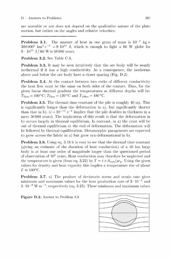
D . Answers to Problems 397

are unstable or not does not depend on the qualitative nature of the plate motion, but rather on the angles and relative velocities.

Problem 3.1. The amount of heat in one gram of mass is 10- 3 kg X

3000002 km2 s-z =9.1013 J , which is enough to light a 60 W globe for 9 · 1013 J /60 W ~ 48 000 years.

Problem 3.2. See Table C.8.

Problem 3.3. It may be seen intuitively that the ore body will be nearly isothermal if it has a high conductivity. As a consequence, the isotherms above and below the ore body have a closer spacing (Fig. D.2).

Problem 3.4. At the contact between two rocks of different conductivity the heat flow must be the same on both sides of the contact. Thus , for the given linear thermal gradient the temperatures at different depths will be: T5km = 100°C; T7km = 120°C and TlOkm = 180°C.

Problem 3.5. The thermal time constant of the pile is roughly 40 my. This is significantly longer than the deformation in a), but significantly shorter than that in b). (E = 10- 12 S- 1 implies that the pile doubles in thickness in a mere 30000 years). The implication of this result is that the deformation in b) occurs largely in thermal equilibrium. In contrast , in a) the crust will be out of thermal equilibrium at the end of deformation. The deformation will be followed by thermal equilibration. Metamorphic parageneses are expected to grow acTOSS the fabric in a) but grow syn-deformational in b) .

Problem 3.6. Using eq. 3.18 it is easy to see that the thermal time constant (giving an estimate of the duration of heat conduction) of a 10 km large body is at least one order of magnitude longer than the questioned period of observation of 105 years. Heat conduction may therefore be neglected and the temperature is given (from eq. 3.22) by T = t x Srad/ pCp. Using the given values for density and heat capacity this implies a temperature rise of about T ~ 100°C.

Problem 3.7. a) The product of deviatoric stress and strain rate gives minimum and maximum values for the heat production rate of 3· 10- 5 and 3.10- 8 W m -3 , respectively (eq. 3.25). These minimum and maximum values

Figure D.2. Answer to Problem 3.3

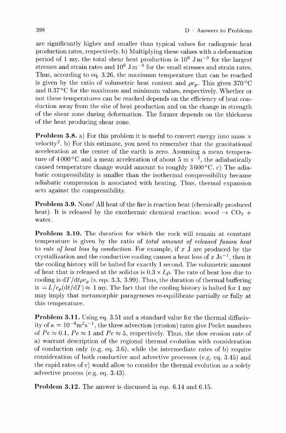
398 D . Answers to Problems

are significantly higher and smaller than typical values for radiogenic heat production rates, respectively. b) Multiplying these values with a deformation period of 1 my, the total shear heat production is 109 J m- 3 for the largest stresses and strain rates and 106 J m -3 for the small stresses and strain rates. Thus, according to eq. 3.26, the maximum temperature that can be reached is given by the ratio of volumetric heat content and pCp. This gives 370 DC and 0.37 D C for the maximum and minimum values, respectively. Whether or not these temperatures can be reached depends on the efficiency of heat con­duction away from the site of heat production and on the change in strength of the shear zone during deformation. The former depends on the thickness of the heat producing shear zone.

Problem 3.8. a) For this problem it is useful to convert energy into mass x velocity2. b) For this estimate, you need to remember that the gravitational acceleration at the center of the earth is zero. Assuming a mean tempera­ture of 4000 DC and a mean acceleration of about 5 m S-2, the adiabatically caused temperature change would amount to roughly 3600 D C. c) The adia­batic compressibility is smaller than the isothermal compressibility because adiabatic compression is associated with heating. Thus, thermal expansion acts against the compressibility.

Problem 3.9. None! All heat of the fire is reaction heat (chemically produced heat). It is released by the exothermic chemical reaction: wood -+ CO2 + water.

Problem 3.10. The duration for which the rock will remain at constant temperature is given by the ratio of total amount of released fusion heat to rate of heat loss by conduction. For example, if x .1 are produced by the crystallization and the conductive cooling causes a heat loss of x .1s-1 , then it the cooling history will be halted for exactly 1 second. The volumetric amount of heat that is released at the solidus is 0.3 x Lp. The rate of heat loss due to cooling is dT /dtpcp (s. eqs. 3.3, 3.99). Thus, the duration of thermal buffering is = L/cp(dt/dT) ~ 1 my. The fact that the cooling history is halted for 1 my may imply that metamorphic parageneses re-equilibrate partially or fully at this temperature.

Problem 3.11. Using eq. 3.51 and a standard value for the thermal diffusiv­ity of", = 1O-6m2s-1 , the three advection (erosion) rates give Peclet numbers of Pe ~ 0.1, Pe ~ 1 and Pe ~ 5, respectively. Thus, the slow erosion rate of a) warrant description of the regional thermal evolution with consideration of conduction only (e.g. eq. 3.6), while the intermediate rates of b) require consideration of both conductive and advective processes (e.g. cq. 3.45) and the rapid rates of c) would allow to consider the thermal evolution as a solely advective process (e.g. eq. 3.43).

Problem 3.12. The answer is discussed in eqs. 6.14 and 6.15.

D . Answers to Problems

Figure D.3. Answer to Problem 3.15b. Curves are labeled in mWm- 2

399

2

1.5

05 -----30

, ----0,5 1.5 2

fe

Problem 3.13. The total amount of heat produced by the crust in model b in Fig. 3.16 is: SOZrad. The question requires that the depth integrated heat production above the depth Zw in model c (eq. 3.67) corresponds to this value. Thus: SOZrad = J;w Soe- z / hr . Integration and inserting the boundaries gives: SOZrad = Sohr (1- e(-zw/hr)). Using hr = 2Zrad we arrive at: 0.5 = e- zw /(2Z rad) or: Zw = 1.38zrad·

Problem 3.14. After inserting the cosine-shaped distribution of heat sources in the crust into eq. 3.56 a first integration gives:

dT Sozc . k dz = -Soz + 41f sm (21fz/ zc) + C1

The first integration constant has the value C1 = qm + SOze, so that the boundary condition kdT / dz = qm at Z = Zc is fulfilled. A second integration gives the result:

T = Sozcz + qm z _ SOZ2 _ Soz~ cos (21fZ) + C2 2k k 4k 8k1f2 Zc

The second constant of integration has the value C2 = Soz~ /(8k1f2), so that T = 0 at Z = o. The given heat source distribution describes a maximum crustal heat production in the center of the crust. This situation could arise if a crust with a "normal" heat source distribution (decreasing with depth) is overthrust by a thick pile of rocks with little heat production ..

Problem 3.15. a) The derivative of eq. 3.76 with respect to Z is:

dT = TI + fchrSoe-z/Uchrl + {;h;So (e-~ _ 1) dz Ilzl fizi

The mantle heat flow may be found by multiplying this equation with k and evaluating it at Z = Zc. b) is solved in Fig. D.3. c) The mantle heat

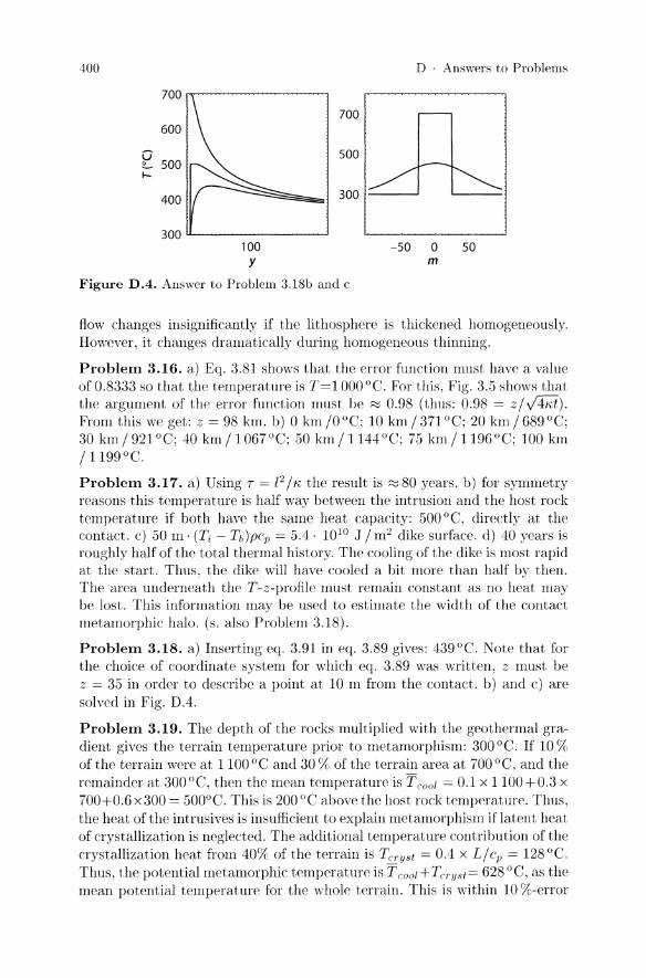
400

G e-I-

700

600

500

400

300 lL-______ ......-J

100 Y

700

500

300

Figure D.4. Answer to Problem 3.18b and c

D . Answers to Problems

-50 0 50 m

flow changes insignificantly if the lithosphere is thickened homogeneously. However, it changes dramatically during homogeneous thinning.

Problem 3.16. a) Eq. 3.81 shows that the error function must have a value of 0.8333 so that the temperature is T=l 000 DC. For this, Fig. 3.5 shows that the argument of the error function must be :::::: 0.98 (thus: 0.98 = z/y'![fd). From this we get: z = 98 km. b) 0 km /0 DC; 10 km / 371 DC; 20 km / 689 DC; 30 km / 921 DC; 40 km /1 067 DC; 50 km /1144 DC; 75 km /1196 DC; 100 km /1199 D C.

Pro blem 3.17 . a) Using T = l2 / '" the result is :::::: 80 years. b) for symmetry reasons this temperature is half way between the intrusion and the host rock temperature if both have the same heat capacity: 500 DC, directly at the contact. c) 50 m· (Ti - Tb)pCp = 5.4· lOlD J / m2 dike surface. d) 40 years is roughly half of the total thermal history. The cooling of the dike is most rapid at the start. Thus, the dike will have cooled a bit more than half by then. The area underneath the T-z-profile must remain constant as no heat may be lost. This information may be used to estimate the width of the contact metamorphic halo. (s. also Problem 3.18).

Problem 3.18. a) Inserting eq. 3.91 in eq. 3.89 gives: 439 D C. Note that for the choice of coordinate system for which eq. 3.89 was written, z must be z = 35 in order to describe a point at 10 m from the contact. b) and c) are solved in Fig. D.4.

Problem 3.19. The depth of the rocks multiplied with the geothermal gra­dient gives the terrain temperature prior to metamorphism: 300 DC. If 10 % of the terrain were at 1100 DC and 30 % of the terrain area at 700 DC, and the remainder at 300 D C, then the mean temperature is Teool = 0.1 x 1100+0.3 x 700+0.6 x 300 = 500DC. This is 200 DC above the host rock temperature. Thus, the heat of the intrusives is insufficient to explain metamorphism if latent heat of crystallization is neglected. The additional temperature contribution of the crystallization heat from 40% of the terrain is Terysf = 0.4 x L/cp = 128 D C. Thus, the potential metamorphic temperature is Tcool+ Teryst= 628 °C, as the mean potential temperature for the whole terrain. This is within 10 %-error

D . Answers to Problems

Figure D.5. Solution of Prob­lem 3.19

I-

~ 1000 ... III

~ ~ 800 ~

600

400

200

o

401

- Mafic / Intrusion

Granitic Heal content of terrain

Intrusion During metamorphis,m

/ / Moo" , ." '","' of intruSive!

I /

He,ll content prior to metamorphism

o 20 40 60 80 100 Areal proportion of terrain (%)

of the observed metamorphic temperature. Contact metamorphism is there­fore a plausible model explanation for the observations . Fig. D.5 illustrates the problem answer graphically.

Problem 3.20. The depths and temperatures of the starting condition are: z[I]=O, T [I ] =O; z [2]= 10 km, T[2]=125 DC; z[3]=20 km, T[3]=250 DC; z[4] = 30 km, T[4] = 375 DC; z[5] = 40 krn, T[5] = 500 DC ; Z[6] = 50 km, T[6] = 0 DC ; z[7] = 60 krn , T[7] = 125 DC ; z [8] = 70 km, T[8] = 250 DC; Z[9] = 80 km, T[9] = 375 DC; z[10] = 90 km, T[10] = 500 DC . The time stepping must be smaller than 0.7937 my. In order to perform the calculations wit.h a round number it is useful to use something like L1t = 0.5 my = 1.575· 101:3 s, i. e. R = 0.1575. After 1L1t the temperatures are: T[5] = 402 DC and T[6] = 98 DC. After 2L1t the temperatures are: T[4] = 360 DC, T[5] = 350 DC, T[6] = 150 DC and T[7] = 140°C. All other temperatures remain up to this time constant because there is no spatial curvature of the temperature profile around them (eq. 3.6) .

Problem 4.1. Using eq. 4.2 we get a distance of the summit of Mt Everest of 6382.207 km from the center of the eart.h and 6384.32 km for Chimborazzo. Thus, Chimborazzo is actually about 2 100 m higher than Everest , if measured from the enter of the earth.

Problem 4.2. In contrast to Fig. 4.5 this diagram is defined for all positive values of fc and fIllI. Homogeneous thickening of the lithosphere is represented by a diagonal line through the diagram. Thickening- of t.he mantle part of the lithosphere with no change of crust.al thickness is represent.ed by a line parallel to the fllll-axis. Crustal thickening at constant thickness of the entire lithosphere must be accompanied by a corresponding thinning of the mantle

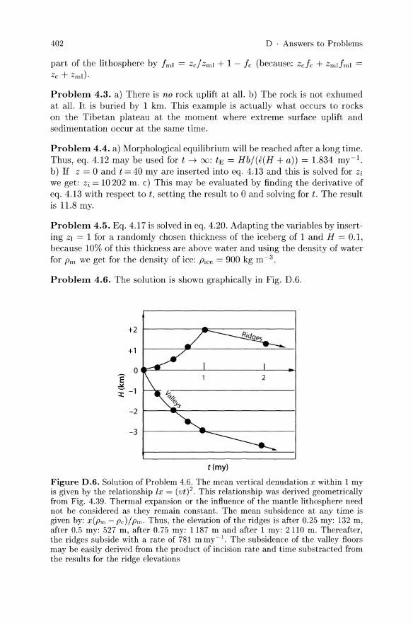
402 D . Answers to Problems

part of the lithosphere by Iml = ZclZml + 1 - Ie (because: zc!c + ZmJ/ml = Zc + Zml).

Problem 4.3. a) There is no rock uplift at all. b) The rock is not exhumed at all. It is buried by 1 km. This example is actually what occurs to rocks on the Tibetan plateau at the moment where extreme surface uplift and sedimentation occur at the same time.

Problem 4.4. a) Morphological equilibrium will be reached after a long time. Thus, eq. 4.12 may be used for t --7 00: tE = Hbj(f(H + a)) = 1.834 my-I. b) If Z = 0 and t=40 my are inserted into eq. 4.13 and this is solved for Zi

we get: Zi = 10202 m. c) This may be evaluated by finding the derivative of eq. 4.13 with respect to t, setting the result to 0 and solving for t. The result is 11.8 my.

Problem 4.5. Eq. 4.17 is solved in eq. 4.20. Adapting the variables by insert­ing Zl = 1 for a randomly chosen thickness of the iceberg of 1 and H = 0.1, because 10% of this thickness are above water and using the density of water for Pm we get for the density of ice: Pice = 900 kg m -3.

Problem 4.6. The solution is shown graphically in Fig. D.6.

+2

+1

O-==c.-.----1...--------'--~

-2

-3

t(my)

Figure D.6. Solution of Problem 4.6. The mean vertical denudation x within 1 my is given by the relationship lx = (vt? This relationship was derived geometrically from Fig. 4.39. Thermal expansion or the influence of the mantle lithosphere need not be considered as they remain constant. The mean subsidence at any time is given by: X(Pm - Pc)/ pm. Thus, the elevation of the ridges is after 0.25 my: 132 m, after 0.5 my: 527 m, after 0.75 my: 1187 m and after 1 my: 2110 m. Thereafter, the ridges subside with a rate of 781 mmy-l. The subsidence of the valley floors may be easily derived from the product of incision rate and time substracted from the results for the ridge elevations

D . Answers to Problems 403

Problem 4.7. a) iJ.H = 10 km (Pm - Pu) / Pm = 937 m. Density and thickness of the crust do not change and therefore need not be considered. b) iJ.H = 391 m. c) the thinning of the crust in b) causes a subsidence of (fe -l)(Pm -Pc) / PmZc = 2343 m. This is partially balanced by an uplift of 391 m by the basaltic underplate. Relative to a) there is a total elevation difference of 937 + (2343 - 391) = 2889 m.

Problem 4.8. The relative importance of thermal expansion and material differences is given directly by the parameters i5 and ~. With the given values these are: i5 = 0.1563 and ~ = 0.018. Thus thermal expansion accounts for roughly 12 % of the density contrast between lithosphere and asthenosphere. However, thermal expansion (or contraction) concerns the entire lithosphere, while the material difference to the asthenosphere exists only in the crust. Thus, because the lithosphere is roughly three times as thick as the crust, thermal contraction accounts for up to 40 % of the surface elevation of a mountain belts in isostatic equilibrium. In lithospheres with thin crust or very thick mantle lithosphere the importance of thermal contraction may even outweigh material differences.

Problem 4.9. a) The answer is: 2.5 cm y~1. From this and the given data the water depths are: 469, 878, 1049, 1483, 1 756, 1906,2392,2633,2795, 2930, 3318, 3709, 3855 and 3995 m for the given distances from the mid oceanic ridge. b) These model values correspond well with the observed values up to an age of roughly 100 my. From there on, sedimentary loading of the plate, its increasing strength and changes of the lower boundary condition by mantle convection cause the divergence between model and observation.

Problem 4.10. a) The units of Dare Nm. The fourth derivative has the units of m~4 and q has the units of stress or force per area. The load is the vertical stress. Fhas therefore the units of N m~ 1, or Newton per meter length of orogen. b) Dh=lOkm ~ 8.8 X 1021 Nm and D h =70km ~ 3 X 1024 Nm.

Problem 4.11. a) The given hints are required to determine the constants of integration. For the first and second integration they the constants must be: C1 = -qL/ D and: C2 = qL2 /(2D), respectively. For the third and fourth integration the constants must be: C3 = 0 and C4 = 0, respectively. Thus: w = qx2 /D(x2 /24-Lx/6+L2 /4). b) At x = L the deflection is: w = 3qL4/(24D). Using the parameters given in the problem we get: D = 0.0008 Nm.

Problem 4.12. a) For the lowest point where there is a density difference between the two columns we can write: column A: O"zz = Pcg(H + Zc + w); column B: O"zz = Pcgzc + pmgw. The buoyancy is given by the difference between these two values. This is the origin of eq. 4.44. b) If the load is qa is not considered, then we can write for the downward force per unit area: (Pc - Pw )wg,.and for the upward directed force: (Pm - Pc)wg. The net force per unit area is therefore: wg(pw - Pm). The total load is: q = qa + wg(pw - Pm).

404 D . Answers to Problems

Problem 4.13. a ~ 65 km.

Problem 4.14. At the highest point of the elastic bulge the slope of the plate is dw / dx = O. The slope of the plate as a function of distance is given by the first spatial derivative of eq. 4.48. If this is set to zero: o = -2wo/ae-x/Oisin(x/a), we get: x = wa. This is the highest point of the fore bulge. In 250 km distance from this point we get from eq. 4.47: D = 2.2· 1023 Nm, and eq. 4.43: h ~ 33 km. The value of Wo does not change the distance of the fore bulge from the load and its knowledge is therefore not required.

Problem 4.15. The problem is easiest solved by plotting the data and graph­ing eq. 4.61 iteratively for different times until a best fit for the data is found. For this a half height of the scarp a ~ 7m should be used, which is roughly half the elevation difference between base and top. It is also useful to subtract roughly 150m from all x values so that the inflection point of the scarp is at x = O. Then, a best fit gives an age of about 30000 years.

Problem 4.16. The two boulders have been exposed to weathering for the same time. This result is easiest arrived at by measuring l (for example in millimeters) off the photograph for the two different boulders and comparing the topographic shapes of the boulders with plots of eq. 4.63. Neither the magnitude of D, not the actual length of l need be known as we perform only a comparison between the two profiles.

Problem 4.17. In the steady state, eq. 4.64 simplifies to Dd2 H /dx2 =- vro . A first integration renders dH /dx=- vroxj D+C1 • C1 • As dH /dx=O at x = o. A second integration renders H = -vro x 2 /(2D)+C2 , where C2 is determined by the boundary condition H = 0 at x = l. The result is H = vro /(2D) x (l2_X2 )

which is actually the first term of eq. 4.65. Evaluating this at x = 0 for the parameter values in Fig. 4.30b we can see that the steady state elevation of the crest above the streams is about 800 m, so that the plotted age of 30000 years is already practically in steady state.

Problem 4.18. According to eq. 4.73 the fractal dimension of the object shown in Fig. 4.41 is: D = log3/log2 = 1.585.

Problem 5.1. The stretch is 2, the elongation is 1. The vertical strain is 100%.

Problem 5.2. Force = mass x acceleration. As weight is a force and the ac­celeration on the surface of the earth is g=9.81 m/ S2, a mass of 1 kg hat has the weight of: 1 kg· 9.81 m/s2 = 9.81 N.

Problem 5.3. Energy is given by the product of force times distance. Thus, the collision process releases 1013N x 105 m = 1018 J. The most important forms of energy into which this mechanical energy is transformed are frictional

D . Answers to Problems 405

heat and potential energy of the mountain belt that formed in response to the collision.

Problem 5.4. As there are no shear stresses and the problem is two di­mensional, we can assume that azz = a1 and axx = a2 (there is no a3). For the continent that is pulled apart by the subducting plate we can write: axx = a2 = -A and azz = a1 = o. From this, the mean stress (pressure) is: am = -A/2. According to eq. 5.11 the vertical and horizontal components of deviatoric stress are: + A/2 and - A/2, respectively. For the continent that collapses under the weight of a mountain range we can write: axx = a3 = 0 and azz = a1 = A. From this, the mean stress is given by: am = A/2. The vertical and horizontal components of deviatoric stress are also: + A/2 and - A/2. Thus, we can conclude that state of deviatoric stress is the same in both continents but the pressure is different.

Problem 5.5. As no shear stresses apply to the surfaces of the rock, all components of eq. 5.16 that describe shear stresses are zero. Eq. 5.16 sim­plifies to: dazz/dz = pg. The corresponding equations for the other two spatial directions in which there is no gravitational acceleration simplify to: daxx/dx = 0 and dayy/dy = O. Integration of these three equation gives: axx = G1, ayy = G2 and azz = pgz + G3. G1, G2 and G3 are the con­stants of integration. They are determined by the boundary conditions of the problem. The normal stresses can be assumed to be zero on each free surface (Fig. 5.34): azz = 0 at z = -H. From this we get: G3 = pgH and azz = pg(H +z). Furthermore, because there is no stresses on the sides it must be true that: G2 = G1 = 0; axx = ayy = o. The mean principal stress (pres­sure P) as a function of depth is: P = (axx + ayy + azz )/3 = pg(H + z)/3. The principal components of the deviatoric stress tensor are, according to eq. 5.9: axx - P = ayy - P = -pg(H + z)/3 and azz - P = 2pg(H + z)/3.

Problem 5.6. Similar to problem 5.5, integration of the stress balance equa­tions gives: axx = G1; ayy = C2 and azz = pgz + C3. As fluids support only negligible differential stresses it is true that: axx = ayy = azz . With the same boundary condition for the vertical component of stress as in Problem 5.5 we get: axx = ayy = azz = pg(z + H) = P. Thus, at any given depth, the pressure in the fluid is three times as high as it is in the rock of Problem 5.5. All components of the deviatoric stress tensor are zero.

Problem 5.7. If the rock can flow apart without resistance, then it must be true that: axx = O. Thus, axx=O, Txx = axx - P = -pg(H + z)/3 and according to eq. 5.37, the horizontal strain rate is: Exx = -pg(z + H)/(6rJ). The rock flows quickly at its base and not at all at its top surface (z = -H). The vertical strain rate is Ezz = pg(z + H)/(3rJ) as Tzz = azz - P = 2pg(H + z)/3.

Problem 5.8. If the side wall is fixed, then the stain rate is: E = 0 and azz = axx . The mean force per area is given by the vertically integrated

406 D . Answers to Problems

vertical stresses py (z + H) using the limits of integration - Hand 0 from Fb = pyH2/2. The mean horizontal stress u xx is therefore u xx = Fbi H = pyHl2.

Problem 5.9. In the fluid: O"xx = O"yy = O"zz = P = Pmyz. In the rock the horizontal stresses for z < 0 are: O"xx = O"yy = 0, and for z > 0 they are: O"xx = O"yy = Pmyz. The vertical stresses in the whole rock are: O"zz = Pcg(H + z). The pressure in the rock is given by the mean of the principal stresses. For z < 0 it is: P = (Pcy(H + z))/3. For z > 0 it is: P = (2pmYz + Pcg(H + z))/3. All principal components of the deviatoric stress tensor in the fluid are O. In the rock, for z < 0 they are: Txx = Tyy = O"xx - P = O"yy -P = -(Pcy(H +z))/3 and: T zz = O"zz -P = (2Pcy(H +z))/3. For z > 0 they are: Txx = Tyy = O"xx - P = O"yy - P = (PmYz - PcY(z + H))/3 and T zz = O"zz - P = -(2PmYz - 2pcY(z + H))/3.

Problem 5.10. From eq. 5.11 we get: E = 0"1 E = 5· 107 Pa/5· 1010Pa = 0.001 = 0.1 %.

Problem 5.11. The vertical stress at any given depth is: O"ZZ = pgz. The strain of a unity cube at depth z in the lithosphere is therefore: E = pyz IE. From this, the total strain integrated over the entire lithosphere is given by: Joz / pyz I Edz = pgz2/2E. Using the given numerical values for the parameters this is: 2500 m. Thus, the elastic thickness change of the total lithosphere due to its own weight is roughly 2.5 % of its total thickness.

Problem 5.12. The solution is graphically shown in Fig. D.7.

a,b c d

Figure D.7. Solution of Problem 5.12

Problem 5.13. For the quartz data the stresses are O"d = 117 MPa; O"d = 24 MPa and O"d = 11 MPa, for n = 2, n = 3 and n = 4, respectively. For olivine the stresses are O"d = 1.4 X 108 MPapd = 2.7 x 105 MPa and O"d = 1.2 X 104 MPa, for n = 2, n = 3 and n = 3, respectively.

Problem 5.14. When taking the logarithm of eq. 5.41 it becomes linear. It then has the form: log(E=nlog(O"d) + log(A)-Q I RT. Thus, if the experimental results are plotted in a diagram of log(f) against log(O"d) the slope of the data gives the power law exponent n and the intercept is (log( A )-Q I RT). Replotting the data from a constant stress on a diagram of log(E against liT

D . Answers to Problems

Figure D.B. Graphical solution of Problem 5.20

407

gives a line with the slope of -Q / R from which the activation energy may be determined.

Problem 5.15. It is because in oceanic lithosphere olivine dominates the lithospheric rheology at much shallower levels (and therefore colder temper­atures) than in continental lithosphere.

Problem 5.16. According to eq. 5.45 it is: Ep = JO-H azzdz = Jo- H pg(H +

z)dz = pgH2/2.

Problem 5.17. The solution is Fb ~ 10.5 X 1012 N m-1 . The result is the same as that from Problem 5.20 as can also be seen from Fig. D.8

Problem 5.18. Eq. 5.52 gives a buoyancy force of Fb ~ 6.6 X 1012 N m-1 .

Problem 5.19. Inserting the given values into eq. 5.54 give a horizontal buoyancy force of the mountain range of Fb ~ 7.71 X 1012 N m -1 . This result may also be read from Fig. 5.32. There, the point Ie = 2, II = 1 gives a value of about Fb ~8.3 X1012 N m -1 . The difference arises from slightly different assumptions of the densities and thicknesses. The result is larger than that from eq. 5.52 because the refined equation (eq. 5.54) also considers thermal contraction of the mantle part of the lithosphere.

Problem 5.20. The graphical solution of this problem is shown in Fig. D.8. The net force between the two columns corresponds to the shaded area on this figure (see also Problem 5.17). Calculating this area algebraically, gives a net force of 10.5. 1012 N m -1 towards the homogeneously thickened lithosphere. This is comparable to the magnitude of plate tectonic driving forces , even though there is no elevation difference between the two lithospheric columns.

Problem 5.21. The kinetic energy (Ekin = mv2 /2) of the plate is: E kin = 3· 102°kg· (0.03 mjy)2 = 271 J (or kg m2 S- I). The potential energy per cubic meter is: Ep = pgh. Thus, with a kinetic energy of 271 J we can lift one cubic meter of rock (using p = 2700 kgm- 3 and 9 = 10 ms- 2 ) merely by about

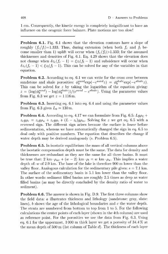
408 D . Answers to Problems

1 cm. Consequently, the kinetic energy is completely insignificant to have an influence on the orogenic force balance. Plate motions are too slow!

Problem 6.1. Fig. 6.1 shows that the elevation contours have a slope of roughly (fel 11)=1.333. Thus, during extension (when both Ie and II be­come smaller than 1) uplift will occur when (fe/II»1.333; for the assumed thicknesses and densities of Fig. 6.1. Eq. 4.29 shows that the elevation does not change when 8ze(fe - 1) = ~zl(f1 - 1) and subsidence will occur when 8ze(fe - 1) < ~zl(f1 - 1). This can be solved for any of the variables in that equation.

Problem 6.2. According to eq. 6.1 we can write for the cross over between sandstone and shale porosities: <Poandexp( _csand z) = <pohaleexp( _cshale z). This can be solved for z by taking the logarithm of the equation giving: z = (log(<poand ) - log(<pohale))/(csand - cshale). Using the parameter values from Fig. 6.3 we get z = 1116 m.

Problem 6.3. Inserting eq. 6.1 into eq. 6.4 and using the parameter values from Fig. 6.3 gives Lo = 130 m.

Problem 6.4. According to eq. 4.17 we can formulate from Fig. 6.5: LgpL + zegPe = zsgpw + zegPe + (L - zs)gPm. Solving for z we get eq. 6.5 with a reversed sign. The different sign arises because the surface is lower before sedimentation, whereas we have automatically changed the sign in eq. 6.5 to deal only with positive numbers. The equation that describes the change if water depth may be derived analogously (s. Problem 6.5).

Problem 6.5. In isostatic equilibrium the mass of all vertical columns above the isostatic compensation depth must be the same. The data for density and thicknesses are redundant as they are the same for all three basins. It must be true that: 2 km· Pair + (w - 2) km· PI = w km· Pw. This implies a water depth of: w of 2.9 km. The base of the lake is therefore 900 m lower than the valley floor. Analogous calculation for the sedimentary pile gives: s = 7.1 km. The surface of the sedimentary basin is 5.1 km lower than the valley floor. In other words: sediment filled basins are roughly 2.5 times as deep as water filled basins (as may be directly concluded by the density ratio of water to sediment).

Problem 6.6. The answer is shown in Fig. D.9. The first three columns show the field data: a illustrates thickness and lithology (sandstone: gray, slate: lines), b shows the age of the lithological boundaries and c the water depth. The strata are numbered from bottom to top from 1 to 5. For the following calculations the center points of each layer (shown in the 4th column) are used as reference point. For the porosities we use the data from Fig. 6.3. Using eq. 6.1 for the uppermost, 1000 m thick layer we get a porosity of 34.4 % at the mean depth of 500 m (1st column of Table d). The thickness of each layer

D . Answers to Problems 409

is based on field measurements and their densities are given by eq. 6.7. In the second column the data for porosity, thickness and density after removal of the uppermost layer (i = 5) are plotted. For the second layer from the top (i = 4) that has a mean depth of 1250 m, we begin with a determination of porosity. Its decompacted thickness is then calculated with eq. 6.4 using the porosities of the first column and the de compacted porosities. The porosity of the third layer after removing the first two strata is given by eq. 6.1 at a depth of 655 m + 500 m and so on. The same principle is repeated for all columns using always the data from the fist column so that no methodical errors are propagated. The sum of the thicknesses and densities if the profile (in the bottom row) are calculated with eq. 6.8 and 6.9. e is a graphical illustration of the data from Table d.

Problem 6.7. To determine the ratio we take the subsidence in eq. 6.10 to be zero, i.e.: H=O. Thus, after rearranging: zelzi = PlaTI/(2(PI - Pw)). For the given numerical values of the parameters: Ze/ZI = 13.7 km. At smaller starting ratios of the thicknesses, the contribution of the mantle part of the lithosphere is so large, so that homogeneous stretching of the lithosphere (when thinned) will lead to surface uplift.

Problem 6.S. Eq. 6.11 shows that the duration of the thermal sag period is only determined by the ratio t / T in the last term of the equation. The time scale of thermal equilibration T is the same we have discussed in eq.3.18 and Table 3.2. It differs from that only by the factor 11"2, but is in principle equivalent. We can see that when t = T, then Hsag has reached (1 - e- I ) x 100% completion. 90% of the thermal sag is completed when: (l_e- t / T ) = 0.9 or: t = -Tln(O.l). This is ~ 75 my for 100 km thick lithosphere and ~ 300 my for 200 km thick lithosphere.

Problem 6.9. For the thickened lithosphere we can use eq. 6.15. We get: qs = 0.06 Wm-2 ; qs = 0.075 Wm-2 and qs = 0.09 Wm- 2 , for the three heat source distributions, respectively. For the thinned lithosphere we must use qs = 2qm + qrad/2 and get: qs = 0.0525 Wm-2 ; qs = 0.075 Wm- 2 and qs = 0.0975 Wm-2 , respectively. We can see that the first distribution results in an increase of the surface heat flow with increasing thickness, while the last distribution results in a decrease of the surface heat flow with increasing thickness.

Problem 6.10. (a) Fig. 5.32 shows that the buoyancy force Fb balances the driving force roughly at Ie ~ 1.65 (while II = 1). Fig. 4.16 shows that this corresponds to a surface elevation of about H ~ 3.5 km. (b) In order to use eq. 5.52, the thickness of the root w must be substituted by w = H pel i1p. It then can be solved for to give H = 4400 m at a buoyancy force of Fb = Fd=5 .1012 N m- I . (c) Eq. 5.54 simplifies significantly for Ii = 1. It then can be used to derive Ie = 1.7 to give Fb = Fd = 5 . 1012 N m -1. From this, eq. 4.25 gives a surface elevation of H = 3800 m. The estimate from (b) is substantially higher than those from (a) and (c) because the thermal contraction in the mantle part of the lithosphere is not considered here.

410

a b c 0

i=5

1000 15 f-i=4-

30

2000 i=3

3000 ~i=2=

40

55

4000

i=l

5000

6000 60

60 50

D . Answers to Problems

d

SOQ..... 34.4 t 1000

2.08 p

12SQ.... 26.8 44.1 t 500 655 2.26 1.96 p

200Q.... 21.9 28.3 34.0 t 1000 1089 1183 2.29 2.18 2.09 p

27SQ.... 12.6 18.4 24.2 43.3 t 500 535 576 770 2.50 2.40 2.30 1.97 p

4S0Q.... 10.4 12.9 14.9 19.8 24.1 II 3000 3086 3156 3384 3577

2.48 2.44 2.40 2.32 2.14

6000 5365 4915 4154 3577 II 2.32 2.24 2.26 2.14 2.23

e

tectonic subsidence

40 30 my

t p

H pL

Figure D.9. Solution of Problem 6.6

Problem 6.11. Using the parameter values from Table 5.3 and eq. 6.28 gives: Ar(T=400) ~ 0.27 and Ar(T= 400) ~ 15. Thus, deformation in the "colder" oro­gen will be concentrated around the collision zone establishing substantial to­pography and potential energy contrasts, while deformation in the "warmer" orogen will be dissipated over a large region with little topography. However, note that the Argand number is used in geodynamics in order to avoid the use of ill-constrained material constants and temperatures in as much detail as we do here. Thus, it is not generally meaningful to use examples like this one for any quantitative consideration of a real orogen.

D . Answers to Problems 411

Problem 6.12. The lithostatic component of pressure in 10 and 15 km depth will be (Yzz = pgz = 275 and 321 MPa, respectively. The temperature at this depth is 300°C and 450 DC, respectively. The strain rate is: 1/5 my-i. From the power law we get differential stresses of 824 MPa and 40 MPa, respec­tively. According to eq. 6.30 the pressure component related to differential stress in 10 or 15 km depth 412 MPa or 20 MPa, respectively. This means that the non lithostatic component of pressure in 10 km depth may be larger than the stress exerted by burial. In 15 km depth pressure is roughly equal to the vertical normal stress.

Problem 7.1. a) We can insert into eq. 7.1 the values: z = 10000 m; P = 1 atm::::i 105 Pa und 9 ::::i 10 m S-2. This gives a mean density of p=l kgm- 3 .

b) 1 atm::::i 1 bar = 10-3 kbar.

Problem 7.2. One mole of almandine has the volume: Valrnandine = 11.5 J /105

Pa = 1.15.10-4 m3 = 115 cm3 .

Problem 7.3. The cation diffusivities at the 3 temperatures are: D300 ::::i 1.6.10-30 m2 S-1; D.500 ::::i 6.9.10-25 m2 S-1; DlOOO ::::i 1.5.10-18 m2 S-I. All these are many orders of magnitude smaller than the diffusivity of thermal energy. Thus, chemical zoning profiles in minerals will only develop because of the sluggishness of cation diffusion, but not because temperature gradients in a crystal.

Problem 7.4. Similar to problem 7.3 we can use the Arrhenius relationship to obtain a diffusivity of D600 ::::i 4.9.10-23 m2 S-I. Inserting this diffusivity and I =1 mm (being careful to use SI units!) we obtain a time scale of more than 600 million years. This is much longer than the duration of most metamorphic events. We can conclude that 1 mm sized garnets are unlikely to be equilibrated at 600°C by diffusion. Chemically equilibrated garnets of this size must have grown at this temperature.

Problem 7.5. The mean diffusivity between 700°C and 400°C is: D ::::i 1.1.10-22 m2 S-I.

Problem 7.6. a) The thermal maximum. b) Because the activation volume in eq. 7.4 is much smaller than the activation energy Q. c) The uppermost curve in Fig. 7.4a. d) Yes, for example if crustal shortening follows intrusion and contact metamorphism.

Problem 7.7. Inserting the given values into eq. 7.9 gives a cooling rate: S ::::i 42°C my-I.

Problem 7.8. a) The characteristic time sale of cooling (the thermal time constant) of the dike is: 4 . 1012 s. The diffusivities at Ti and Tb are D 1200 ::::i 1.3· 10-14 m2 S-1 and D500 ::::i 7.4· 10-20 m2 S-I. The diffusive time constants of mica are T1200 ::::i 1.9· 109 sand T500 ::::i 3.35· 1014 s. Thus,

412 D . Answers to Problems

the chemical equilibration of the micas is much more rapid than the cooling of the dike at 1 200 ° C but much slower than the cooling at 500 ° C. Thus, it may be - in principal - meaningful to use the micas to determine the in­trusion age geochronologically. However, 50 m from the intrusion contact the maximum contact metamorphic temperatures are much lower than 1200 DC. Thus it is necessary to obtain better information on the contact metamor­phic temperatures to investigate if the dating of these micas is meaningful. b) Eq. 3.91 shows that the maximum contact metamorphic temperature of the micas is reached 2.83· 1011 s after intrusion. Inserting this into eq. 3.89 we get the contact metamorphic peak temperature the micas experienced to be: T max = 829°C. Using this number as the starting temperature TA and 500°C as the final temperature TE , eq. 7.8 may be used to estimate the mean diffusivity to be: D ~ 1.91· 10-17 m2 S-l and T = 1.3· 1012 s. This value is only a bit shorter that the characteristic time scale of cooling of the dike. Thus, equilibration of the micas is likely to be at least affected by the contact metamorphism. Whether the micas are partially or fully equilibrated can not be answered and requires careful analysis.

Problem 7.11. The T-t-curve passes following points: 700°C; 0 my -+ 700°C; 3 my -+ 400 ° C; 6 my -+ 0 ° C; 26 my. However, the last point will not be reached as the cooling curve intersects the stable geotherm before that. The corner points of the z-t-curve are: 20 km; 0 my -+ 14 km; 5 my -+ 0 km; 40 my. The intersection of the cooling curve with the stable geotherm may be found by finding the intersection of the linear equations T =

z x 20°C /km and T = 280°C - z x 50°C /km. It is at: T = 187°C and z = 9333 m. According to these results, the P-T-path follows the following evo­lution: 5.4 kbar; 700°C -+ 4.43 kbar; 700°C -+ 3.78 kbar; 500°C -+ 3.67 kbar; 400°C-+2.52 kbar; 187°C-+0 kbar; O°C.

Problem A.I. The solution of this problem is simply the sum of the ap­proximations from eq. A.13 and eq. A.16:

Problem A.2. The answer is:

-D Wi = Ll 4( ) (Wi+1 - 4Wi+1 - 4Wi-1 + Wi-2)

6D + x Pm - Pc 9

This equation was derived by forming the difference between the curvature at neighboring grid points in an analogous way to the way eq. A.16 was formulated.

Problem A.3. Using u = Llx/Llt forward and backward finite differencing schemes give the following approximations: Ti+ = Ti+1 bzw. Tt = 2Ti- -

D . Answers to Problems 413

Ti-=-l. If you draw these equations according to the scheme of Fig. A.5, it becomes visible that backward differencing schemes become unstable.

Problem AA. Both data sets have a mean of p, = 8. The first data set hgas a variance of Var = 4, but an unbiased estimate of the population variance of Var' =4.57. For the second data set the variance is Var = 42, but the unbiased estimate of the population variance is Var' = 48.

E. Internet Addresses

On the next few pages there is a random selection of internet addresses that are in some way related to geodynamics. The list was not created according to any important selective criteria and obviously claims no completeness. It is merely a number of addresses that were encountered during the writing of this book.

Software and Online Tools:

ANSYS. Commercial FEM package • http://www.ansys.com/

DimensionMG. General purpose 3D mesh generator • http://www.ahpcrc.org/ johnson/SOFTWARE/MESHGEN/

ESRI. widely used GIS software and data depot • http://www.esri.com/

Geo Vu. Software to simplify access to diverse data • http://www.ngdc.noaa.gov/seg/geovu/

GMT. Software to produce maps from digital data (e.g. Fig. 1.2, 1.1) • http://gmt.soest.hawaii.edu/

MARC. Commercial FEM package • http://www.marc.com/

MATLAB. Software to do mathematics • http://www.mathworks.com/products/matlab/

MICRODEM. Software for imaging of digital elevation models • http://www.usna.edu/Users/oceano/pguth/website/microdemdown.htm

Online topographic map creation facility • http://www.aquarius.geomar.de/omc/

Online paleogeographic map creation (Fig. 2.3) • http://www.odsn.de/odsn/services/paleomap/paleomap.html

SCOTESE. Plate and climate reconstruction • http://www.scotese.com/

Spectral analysis of data toolkit • http://www.atmos.ucla.edu/tcd/ssa/

Data Centers, Downloads and Support:

416 E . Internet Addresses

Bathymetry, topography • http://www.ngdc.noaa.gov /mgg/bathymetry /relief.html

Bathymetric chart of the arctic ocean • http://www.ngdc.noaa.gov /mgg/bathymetry /arctic/ arctic.html

Bathymetric chart of the oceans • http://www.ngdc.noaa.gov /mgg/gebco/gebco.html

Digital elevation models for the US • http://mcmcweb.er.usgs.gov

Digital elevation model Etopo5 • http://www.ngdc.noaa.gov /mggfglobal/seltopo.html • http://www .ncgia. ucs b .edu / pu bs / spherekit / platforms.html

Digital elevation model Gtopo30 • http://edcdaac. usgs.gov / gtopo30 / gtopo30.html

Digital elevation model Global Topo 2min • ftp:/ /topex.ucsd.edu/pub/globaLtopo_2min/

Digital elevation model of the US • http://edcwww.cr.usgs.gov/Webglis/glisbin/guide.pl/glis/hyper /guide/7 ...min_de

Earth sciences websites • http://www. websites.noaa.gov / guide/sciences/ earth/ earth.html

Earthquake catalogue • http://quake.geo. berkeley.edu/ cnss /

Earthquake Database • http://www.ngdc.noaa.gov / seg/hazard/ sig...srch.shtml

Geographic data download of USGS. • http://edcwww.cr.usgs.gov/doc/edchome/ndcdb/ndcdb.html

Geological time table • http://www.dinosauria.com/dml/history.htm

Geological time table • http://www.ucmp.berkeley.edu/help/timeform.html

Geomagnetics • http://www.noaa.gov /geomagnetics.html

Geophysical data base of the USGS • http://crustal.cr.usgs.gov /crustal/geophysics/index.html

Geothermal heat flow data • http://www .noaa.gov / geothermal.html

G IS data depot • http://www.gisdatadepot.com/

Gravity land • http://www.noaa.gov /landgravity.html

Gravity data marine (Sandwell) • http://topex.ucsd.edu/marine_grav/maLgrav.html

Gravity data global • ftp:/ /topex.ucsd.edu/pub/globaLgrav_2min/

E . Internet Addresses

Gravimetric data base • http://bgi.cnesJr:8110/bgLservice-B..html

Heavens above cities • http://www.heavens-above.com/countries.asp

IERS. International earth rotation service • http://maia.usno.navy.mil/

IGS. International GPS service • http://tonga.unavco.ucar.edu/

International GPS support association • http://igscb.jpl.nasa.gov /

Landform atlas of the US • http://fermi.jhuapl.edu/states/states.html

Marine geology and geophysics data bases • http://www.ngdc.noaa.gov /mgg/mggonline.html

National geophysical data center of the US • http://www.ngdc.noaa.gov/ngdc.html

Natural hazards • http://www.noaa.gov/hazards.html

Satellite images • http://earth.jsc.nasa.gov / • http://visibleearth.nasa.gov / • http://nix.nasa.gov / • http://www.earthkam.ucsd.edu/ • http://www.spaceimaging.com/index_text.html

Seafloor topography from satellite

417

• http://www .ngdc.noaa.gov / mgg/ announcements / announce-predict .html Sediment thicknesses around the world

• http://www.ngdc.noaa.gov /mgg/sedthick/sedthick.html Seismologic data bases

• http://www.seismology.harvard.edu/CMTsearch.html Shoreline data base

• http://www.ngdc.noaa.gov/mgg/shorelines/gshhs.html Shoreline of the United States

• http://www.csc.noaa.gov/products/shorelines/digdata.htm Statistic data of the world

• http://www.un.org/Depts/unsd/ Topography analysis tools

• http://www.bell-labs.com/project/topo/ World stress map project (Fig. 2.2)

• http http://www-wsm.physik.uni-karlsruhe.de/ World fact book of the CIA

• http://www.odci.gov /cia/publications/factbook/index.html World maps

• http://ortelius.maproom.psu.edu/dcw/

418

Important Earth Science Journals:

Links to a range of journals • http://www.earth.monash.edu.au/Journals.html

Australian Journal of Earth Science (Blackwell)

E . Internet Addresses

• http://www.blacksci.co.uk/products/journals/xajcs.htm Computers and Geoscience (Elsevier)

• http://www.elsevier.com/inca/publications/store/3/9/8/ Earth and Planetary Science Letters (Elsevier)

• http://www.elsevier.nl:80 /inea/publications/store/ 5/0/3/3/2/8/ Earth Science Reviews (Elsevier)

• http://www.elsevier.com/inca/publications/store/ 5 /0 /3/3/2/9 / Electronic Geosciences

• http://link.springer.de/link/service/journals/10069 /index.htm EOS

• http://www.agu.org/pubs/eos.html Geochemistry, Geophysics, Geosystems (electronic journal)

• http://146.201.254.53/ Geophysical Journal International (Blackwell)

• http://www.blacksci.co.uk/products/journals/gji.htm Geophysical Research Letters

• http://www.agu.org/grl/ GSA Bulletin, Geology, GSA today

• http://www.geosociety.org/pubs/ Journal of Applied Geophysics (Elsevier)

• http://www.elsevier.com/inca/publications/store/5 /0 /3/3/3/3/ .I ournal of Geophysical Research

• http://www.agu.org/journals/jb/ Journal of Metamorphic Geology (Australian site)

• http://www.es.mq.edu.au/jmg/jmg.html Journal of African Earth Science (Elsevier)

• http://www.elscvier.com/inca/publications/store/6/9/1/ Journal of Geodynamics (Elsevier)

• http://www.elsevier.com/inca/publications/store/8/7 /4/ Journal of Petrology (Elsevier)

• http://petrology.oupjournals.org/ Journal of Structural Geology (Elsevier)

• http://www.elsevier.nl:80/inca/publications/store/5/3/9/ Journal of the Virtual Explorer (electronic journal)

• http://www.virtualexplorer.com.au/ Mineralogy and Petrology

• http://link.springer.de/link/service/journals/007l0 /indcx.htm Physics of the Earth and Planetrary Interiors

• http://www.elsevier.com/inca/publications/store/5 /0 /3/3/5 /6/

E . Internet Addresses

Precambiran Research (Elsevier) • http://www.elsevier.com/inca/publications/store/5/0/3/3/5/7 /

Reviews in Geophysics • http://www.agu.org/rog/

Tectonics • http://www.agu.org/journals/tc/

Important Geological Organisations:

American Geophysical Union (AGU) • http://www.agu.org/

Austrian Geological Survey • http://www.geolba.ac.at/

Austrian portal to academic institutions home pages • http://www.portal.ac.at/

Australian earth science departments • http://www.earth.monash.edu.au/aus_depts.html

Australian Geological Survey • http://www.agso.gov.au/

British Geological Society • http://www.geolsoc.org.uk

Geological Society of America • http://www.geosociety.org/

German portal to academic Institutions Home pages • http://www.bildungsserver.de/

International Earth Science Departments and Organsiations

419

• http://dir.yahoo.com/Science/Earth..sciences / Geology ..and_Geophysics /Institute~ NASA

• http://www.nasa.gov /NASAJl.Omepage.html/ Swiss portal to academic institutions home pages

• http://www.switch.ch/ European geoscience department listing

• http://www.uni-mainz.de/FB/Geo/Geologie/GeoInst/Europa.html

References

Abramowitz M, Stegun IA (1972) Handbook of mathematical functions with for­mulas, graphs mathematical tables. Dover Publications, New York, 1045 p

Ahnert F (1970) Functional relationships between denudation, relief and uplift in large mid-latitude drainage basins. Am J Sci 268:243-263

Ahnert F (1976) Brief description of a comprehensive three-dimensional process­response model of landform development. Z Geomorphol Suppl 25:29-49

Ahnert F (1984) Local relief and the height limits of mountain ranges. Am J Sci 284:1035-1055

Albers HC (1805) Beschreibung einer neuen Kegelprojektion. Zachs monatliche Korrespondenz zur Beforderung der Erd- und Himmelskunde, Nov:450-459

Allen PA, Allen JR (1990) Basin analysis. Principles and applications. Blackwell Scientific Publication, Oxford, 450 p

Anderson DA, Tannehill JC, Pletcher RH (1984) Computational fluid mechanics and heat transfer. Series in computational methods in mechanics and thermal sciences. McGraw Hill, New York, 599 p

Anderson EM (1951) The dynamics of faulting. Oliver and Boyd, Edinburgh, 206 p

Anderson GM, Crerar DA (1993) Thermodynamics in geochemistry, the equilibrium model. Oxford University Press, Oxford, 588 p

Andrews DJ, Bucknam RG (1987) Finite degradation of shoreline scarps by a non­linear diffusion model. J Geophys Res 92:12857-12867

Angelier J (1984) Tectonic analysis of fault slip data sets. J Geophys Res 89:5835-5848

Angelier J (1994) Fault slip analysis and palaeo-stress reconstruction. In: Hancock P (ed) Continental deformation. Pergamon Press, Oxford, pp 53-101

Angevine CL, Heller PL, Paola C (1990) Quantitative sedimentary basin modelling. AAPG Continuing Education Course Note Series 32, 133 p

Argus DF, Heflin MB (1995) Plate motion and crustal deformation estimated with geodetic data from the Global Positioning System. Geophys Res Lett 22:1973-1976

Armstrong AC (1980) Soils and slopes in a humid environment. Catena 7:327-338 Artyushkov EV (1973) Stresses in the lithosphere caused by crustal thickness inho­

mogenities. J Geophys Res 78:7675-7708 Atkins PW (1994) Physical chemistry, 5th edition. Oxford University Press, Oxford,

1031 p Avigard D (1992) On the exhumation of coesite-bearing rocks in the Dora-Maira

massif (Western Alps, Italy). Geology 18:466-469 Avouac JP (1993) Analysis of scarp profiles: evaluation of errors in morphological

dating. J Geophys Res 98:6745-6754

422 References

A vouac JP, Peltzer G (1993) Active tectopnics in southern Xinjiang, China: Anal­ysis of terrace riser and normal fault scarp degradation along the Hotan-Qira Fault System. J Geophys Res 98:21773-21807

Barr TD, Dahlen FA (1989) Brittle frictional mountain building 2nd thermal struc­ture and heat budget. J Geophys Res 94:3923-3947

Barr TD, Houseman GA (1996) Deformation fields around a fault embedded in a non-linear ductile medium. Geophys J Int 125:473-490

Barrell J (1914) The strength of the Earth's crust. J Geol 22:441-468 Barton CM, England PC (1979) Shear heating at the Olympos (Greece) thrust and

the deformation properties of carbonates at geological strain rates. Geol Soc Am Bull 90:483-492

Barton MD, Hanson RB (1989) Magmatism and the development of low pressure metamorphic belts: implications from the western United States and thermal modelling. Geol Soc Am Bull 101:1051-1065

Bassi G (1991) Factors controlling the style of continental rifting: insights from numerical modelling. Earth Planet Sci Lett 105:430-452

Bassi G, Keen CE, Potter P (1993) Contrasting styles of rifting: models and exam­ples from the eastern Canadian margin. Tectonics 12:639-655

Batt GE, Braun J (1997) On the thermomechanical evolution of compressional orogens. Gephys J Int 128:364-382

Beaumont C (1981) Foreland basins. Geophys J Roy Astron Soc 65:291-329 Beaumont C, Fullsack P, Hamilton J (1992) Erosional control of active compres­

sional orogens. In: McClay KR (ed) Thrust tectonics. Chapman and Hall, New York, pp 1-18

Beaumont C, Ellis S, Hamilton J, Fullsack P (1996) Mechanical model for subduct ion­collision tectonics of Alpine-type compressional orogens. Geology 24: 675-678

Begin SB, Meyer DF, Schumm SA (1981) Development of longitudinal profiles of alluvial channels in response to base level lowering. Earth Surface Processes and Landforms 6:49-68

Bell JS, Gough DI (1979) Northwest-southeast compressive stress in Alberta: evi­dence from oil wells. Earth Planet Sci Lett 45:475-482

Benfield AE (1949) The effect of uplift and denudation on underground tempera­tures. J Appl Phys 20: 66-70

Berman RG (1988) Internally-consistent thermodynamic data for minerals in the system Na20-K2 0-CaO-MgO-FeO-Fe203-Ah03-Si02 - Ti02-H20-C02 • J Pet 29: 445-522

Bickle MJ, McKenzie D (1987) The transport of heat and matter by fluids during metamorphism. Contrib Mineral Petrol 95:384-392

Bickle MJ, Hawkesworth CJ, England PC, Athey D (1975) A preliminary thermal model for regional metamorphism in the eastern Alps. Earth Planet Sci Lett 26:13-28

Bird P (1979) Continental delamination and the Colorado Plateau. J Gephys Res 84:7561-7571

Bird P, Piper K (1980) Plane stress finite element model of tectonic flow in southern California. Phys Earth Planet Int 21:158-195

Blanckenburg F von, Davies JH (1995) Slab breakoff: a model for syncollisional magmatism and tectonics in the Alps. Tectonics 14:120-131

Bohlen SR (1987) Pressure temperature time paths and a tectonic model for the evolution of granulites. J Geol 95:617-632

Bond GC, Kominz MA, Devlin WJ (1983) Thermal subsidence and eustasy in the lower Paleozoic miogeocline of western North America. Nature 306:775-779

Bons PD, Barr TD, ten Brink CE (1997) The development of delta-clasts in non­linear viscous materials: a numerical approach. Tectonophys 270:29-42

References 423

Bott MHP (1993) Modelling the plate-driving mechanism. J Geol Soc London 150:941-951

Bott MHP, Waghorn GD, Whittaker A (1989) Plate boundary forces at subduction zones and trench-arc compression. Tectonophys 170:1-15

Brace WF, Kohlstedt DL (1980) Limits on lithospheric stress imposed by laboratory experiments. J Geophys Res 94:3967-3990

Braun J (1992) Dynamics of compressional orogens; beyond thin sheet and plane strain approximations. EOS tranctions 73:292

Braun J, Beaumont C (1995) Three dimensional numerical experiments of strain partitioning at oblique plate boundaries: Implications for contrasting tectonic styles in the southern coast ranges, California central south island, New Zealand. J Geophys Res 100:18059-18074

Braun J, Sambridge M (1997) Modelling landscape evolution on geological time scales: a new method based on irregular spatial discretization. Basin Res. 9:27-52

Brown RW (1991) Backstacking apatite fission track "stratigraphy": a method for resolving the erosional and isostatic rebound components of tectonic uplift his­tories. Geology 19:74-77

Brun JP, Cobbold PR (1980) Strain heating and thermal softening in continental shear zones: a review. J Struct Geol 2:149-158

Buck WR (1991) Modes of continental lithosphere extension. J Geophys Res 96:20161-20178

Buck WR, Martinez F, Steckler MS, Cochran JR (1988) Thermal consequences of lithosphere extension: pure and simple. Tectonics 7:213-234

Burbank DW, Anderson RS (2001) Tectonic geomorphology. Blackwell Science, Malden, Mass 274 p

Byerlee JD (1968) Brittle ductile transition in rocks. J Geophys Res 73:4741-4750 Byerlee JD (1970) Friction of rocks. In: Everden JF (ed) Experimental studies

of rock friction with application to earthquake prediction. USGS, Menlo Park, pp 55-77

Carey SW (1976) The expanding Earth. Elsevier, Amsterdam, 488 p Carslaw HS, Jaeger JC (1959) Conduction of heat in solids. Oxford Science Publi­

cations, Oxford University Press, Oxford, 510 p Carson CJ, Powell R, Wilson CJL, Dirks PHMG (1997) Partial melting during

tectonic exhumation of a granulite terrain: an example from the Larsemann Hills, East Antarctica. J Met Geol 15:105-127

Carson MA, Kirkby MJ (1972) Hillslope form and processes, Cambridge University Press, Cambridge, 475 p

Chamberlain CP, Sonder LJ (1990) Heat-producing elements and the thermal and baric patterns of metamorphic belts. Science 250:763-769

Chapple WM (1978) Mechanics of thin-skinned fold-and-thrust belts. Geol Soc Am Bull 89:1189-1198

Chase CG (1992) Fluvial landsculpting and the fractal dimension of topography. Geomorphology 5:39-57

Chemenda A, Mattauer M, Bokun AN (1996) Continental subduction and a mech­anism for exhumation of high-pressure metamorphic rocks: new modelling and field data from Oman. Earth Planet Sci Lett 143:173-182

Christensen UR, Yuen DA (1984) The interaction of a subducting lithospheric slab with a chemical or phase boundary. J Geophys Res 89:4389-4402

Christie JM, Ord A (1980) Flow stress from microstructures of mylonites: example and current assessment. J Geophys Res 85:6253-6262

424 References

Cliff RA, Droop GTR, Rex DC (1985) Alpine metamorphism in the south-east Tauern Window, Austria: 2nd Rates of heating, cooling and uplift. J Met Geol 3:403-415

Cloetingh S, van Wees JD, van der Beek PA, Spadini G (1995) Role of pre-rift rheology in kinematics of extensional basin formation: constraints from thermo­mechanical models of Mediterranean and intracratonic basins. Mar Petrol Geol 12:793-807

Cloos M (1982) Flow melanges: numerical modelling and geologic constraints on their origin in the Franciscan subduction complex, California. Bull Geol Soc Am 93:330-345

Cloos M (1984) Flow melanges and the structural evolution of accretionary wedges. Geol Soc Am Spec Pap 198:71·79

Cloos M, Shreve RL (1988) Subduction channel model of accretion, melange forma­tion, sediment subduction and subduction erosion at convergent plate margins 1. Background and description. Pure and Applied Geophys 128:455-500

Coblentz D, Richardson RM, Sandiford M (1994) On the potential energy of the Earth's lithosphere. Tectonics 13:929-945

Coblentz D, Sandiford M (1994) Tectonic stress in the African plate: constraints on the ambient lithospheric stress state. Geology 22:831-834

Cochran JR (1982) The magnetic quite zone in the eastern gulf of Aden: implica­tions for the early development of the continental margin. Geophys J Roy Astron Soc 68:171-202

Cochran JR (1983) Effects of finite extension times on the development of sedimen­tary basins. Earth Planet Sci Lett 66:289-302

Coffin MF, Eldholm 0 (1994) Large igneous provinces: crustal strucutre, dimen­sions, and external consequences. Rev Geophys 32:1··36

Coffin MF (1997) Models for the emplacement of large igenous provinces; a review. In: International lithosphere program on volcanic margins, abstract volume, Ge­oforschungszentrum Potsdam.

Coffin MF, Eldholm 0 (1993a) Scratching the surface: Estimating dimensions of large igeneous provinces. Geology 21:515-518

Coffin MF, Eldholm 0 (1 993b) Large igneous provinces. Scientific American 269: 42-49

Connolly JAD, Thompson AB (1989) Fluid and enthalpy production during re­gional metamorphism. Contrib Mineral Petrol 102:347-366

Conrad CP, Molnar P (1999) Convective instability of a boundary layer with temperature- and strain-rate-dependent viscosity in terms of "abvailable buoy­ancy". Geophys J Int 139:51-68

Cooke RA, OBrian PJ, Carswell DA (2000) Garnet zoning and the identification of equilibrium mineral compositions in high pressure-temperature granulites from the Moldanubian zone, Austria. J Metam Geol 18:551-569

Coulomb CA (1773) Sur une application des n§gles de maximis et minimis a quelques problemes de statique relatifs a l'architecture. Acad Roy Sci Mem de Math et de Phys 7:343-382

Cowan DS, Silling RM (1978) A dynamic scaled model of accretion and trenches and its implications for the tectonic evolution of subduction complexes. J Geophys Res 83:5389-5396

Cox A (1972) Plate tectonics and geomagnetic reversals. Freeman and Company, San Francisco, 702 p

Crank J (1975) The mathematics of diffusion, 2nd edn. Oxford Science Publications. Clarendon Press, Oxford, 414 p

Creager KC, Jordan TH (1984) Slab penetration into the lower mantle. J Geophys Res 89:3031-3050

References 425

Crough ST (1983) Hot spot swells. Ann Rev Earth Planet Sci 11:165-193 Cull JP (1976) The measurement of thermal parameters at high pressures. Pageoph

114:301-307 Culling WEH (1960) Analytical theory of erosion. J Geol 68:336-344 Cygan RT, Lasaga AC (1985) Self-diffusion of magnesium in garnet at 750D C to

900D C. Am J Sci 285:328-350 Dahlen FA (1984) Non-cohesive critical Coulomb wedges: an exact solution. J Geo­

phys Res 89:10125-10133 Dahlen FA, Barr TD (1989) Brittle frictional mountain building 1st Deformation

and mechanical energy budget. J Geophys Res 94:3906-3922 Dahlen FA, Suppe J, Davis D (1984) Mechanics offold-and-thrust belts and accre­

tionary wedges: cohesive coulomb theory. J Geophys Res 89:10087-10101 Dalmayrac B, Molnar P (1981) Parallel thrust and normal faulting in Peru and

constraints on the state of stress. Earth Planet Sci Lett 55:473-481 Davis D, Suppe J, Dahlen FA (1983) Mechanics of fold-and-thrust belts and accre­

tionary wedges. J Geophys Res 88:1153-1172 DeMets C, Gordon RG, Argus DF, Stein S (1990) Current plate motions. Geophys

J Int 101:425-478 Dewey JF (1988) Extensional collapse of orogens. Tectonics 7:1123-1139 DeYoreo JJ, Lux DR, Guidotti CV (1991) Thermal modelling in low-pressure/high­

temperature metamorphic belts. Tectonophys 188:209-238 Dickinson WR (1976) Plate tectonic evolution of sedimentary basins. AAPG Con­

tinuing Education Course Note Series 1:1-62 Dodson MH (1973) Closure temperature in cooling geochronological and petrolog­

ical systems. Contrib Mineral Petrol 40:259-274 Doin, Fleitout (1996) Thermal evolution of the oceanic lithosphere: an alternative

view. Earth Planet Sci Lett 142:121-136 Doglioni C (1993) Some remarks on the origin of foredeeps. Tectonophys 228:1-20 Dunning GH, Etheridge MA, Hobbs BE (1982) On the stress dependence of sub­

grain size. Textures and Microstructures 5:127-152 Edmond JM, Damm K von (1983) HeiBe Quellen am Grund der Ozeane. Spektrum

der Wissenschaft 6:74-87 Ehlers K, Powell R (1994) An empirical modification of Dodson's equation for

closure temperature in binary systems. Geochim Cosmochim Acta 58:241-248 Ehlers K, Powell R, Stiiwe K (1994a) The determination of cooling histories from

garnet-biotite equilibrium. Am Min 79:737-744 Ehlers K, Stiiwe K, Powell R, Sandiford M, Frank W (1994b) Thermometrically

inferred cooling rates from the Plattengneiss, Koralm region, eastern Alps. Earth Planet Sci Lett 125:307-321

Elison MW (1991) Intracontinental contraction in western North America: conti­nuity and episodicity. Geol Soc Am Bull 103:1226-1238

Engelder T (1993) Stress regimes in the lithosphere. Princeton University Press, Princeton, 451 p

Engelder T (1994) Deviatoric stressitis: a virus infecting the Earth science commu­nity. EOS 75:18, 210-213

England PC (1981) Metamorphic pressure estimates and sediment volumes for the Alpine orogeny: an independent control on geobarometers? Earth Planet Sci Lett 56:387-397

England PC (1987) Diffusive continental deformation: length scales, rates and meta­morphic evolution. Phil Trans R Soc Lon 321:3-22

England PC (1996) The mountains will flow. Nature 381:23-24

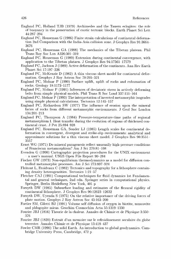
426 References

England PC, Holland TJB (1979) Archimedes and the Tauern eclogites: the role of buoyancy in the preservation of exotic tectonic blocks. Earth Planet Sci Lett 44:287-294

England PC, Houseman G (1986) Finite strain calculations of continental deforma­tion 2nd Comparison with the India-Asia collision zone. J Geophys Res 91:3664-3676

England PC, Houseman GA (1988) The mechanics of the Tibetan plateau. Phil Trans Roy Soc Lon A326:301-319

England PC, Houseman G (1989) Extension during continental convergence, with application to the Tibetan plataeu. J Geophys Res 94:17561-17579

England PC, Jackson J (1989) Active deformation of the continents. Ann Rev Earth Planet Sci 17:197·-226

England PC, McKenzie D (1982) A thin viscous sheet model for continental defor­mation. Geophys J Roy Astron Soc 70:295-321

England PC, Molnar P (1990) Surface uplift, uplift of rocks and exhumation of rocks. Geology 18: 1173-1177

England PC, Molnar P (1991) Inferences of deviatoric stress in actively deforming belts from simple physical models. Phil Trans R Soc Lond 337:151-164

England PC, Molnar P (1993) The interpretation of inverted metamorphic isogrades using simple physical calculations. Tectonics 12:145-157

England PC, Richardson SW (1977) The influence of erosion upon the mineral facies of rocks from different metamorphic environments. J Geol Soc London 134:201-213

England PC, Thompson A (1984) Pressure-temperature-time paths of regional metamorphism I. Heat transfer during the evolution of regions of thickened con­tinental crust. ol Pet 25:894-928

England PC, Houseman GA, Sonder Lol (1985) Length scales for continental de­formation in convergent, divergent and strike-slip environments: analytical and approximate solutions for a thin viscous sheet model. ol Geophys Res 90:3551-3557

Ernst WG (1971) Do mineral paragenesis reflect unusually high-pressure conditions of Franciscan metamorphism? Am ol Sci 270:81-108

Evenden G (1990) Cartographic projection procedures for the UNIX environment - a user's manual. USGS Open File Report 90- 284

Fischer GW (1973) Non-equilibrium thermodynamics as a model for diffusion con­trolled metamorphic processes. Am J Sci 273:897-924

Fleitout L, Froidvaux C (1982) Tectonics and topography for a lithosphere contain­ing density heterogeneities. Tectonics 1:21-57

Fletcher CAol (1991) Computational techniques for fluid dynamics 1st Fundamen­tal and general techniques, 2nd edn. Springer series in computational physics. Springer, Berlin Heidelberg New York, 401 p

Forsyth DW (1985) Subsurface loading and estimates of the flexural rigidity of continental lithosphere. J Geophys Res 90:12623-12632

Forsyth DW, Uyenda S (1975) On the relative importance of the driving forces of plate motion. Geophys ol Roy Astron Soc 43:163--200

Fortier SM, Giletti Bol (1991) Volume self diffusion of oxygen in biotite, muscovite and phlogopite micas. Geochim Cosmochim Acta 55:1319-1330

Fourier olBol (1816) Theorie de la chaleur. Ann ales de Chimie et de Physique 3:350-376

Fourier olBol (1820) Extrait d'un memoire sur Ie refroidissement seculaire du globe terrestre. Annales Chimie et de Physique 13:418-437

Fowler CMR (1990) The solid Earth. An introduction to global geodynamics. Cam­bridge University Press, Cambridge, 472 p

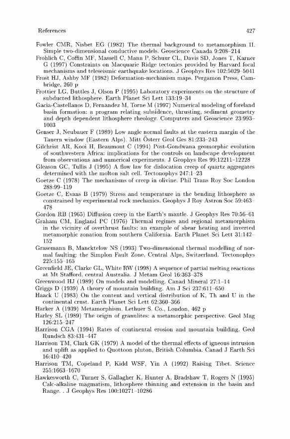
References 427

Fowler CMR, Nisbet EG (1982) The thermal background to metamorphism II. Simple two-dimensional conductive models. Geoscience Canada 9:208-214

Frohlich C, Coffin MF, Massell C, Mann P, Schuur CL, Davis SD, Jones T, Karner G (1997) Constraints on Macquarie Ridge tectonics provided by Harvard focal mechanisms and teleseismic earthquake locations. J Geophys Res 102:5029-5041

Frost HJ, Ashby MF (1982) Deformation-mechanism maps. Pergamon Press, Cam­bridge, 260 p

Frottier LG, Buttles J, Olson P (1995) Laboratory experiments on the structure of subducted lithosphere. Earth Planet Sci Lett 133:19-34

Gacia-Castellanos D, Fernandez M, Torne M (1997) Numerical modeling offoreland basin formation: a program relating subsidence, thrusting, sediment geometry and depth dependent lithosphere rheology. Computers and Geoscience 23:993-1003

Genser J, Neubauer F (1989) Low angle normal faults at the eastern margin of the Tauern window (Eastern Alps). Mitt Osterr Geol Ges 81:233-243

Gilchrist AR, Kooi H, Beaumont C (1994) Post-Gondwana geomorphic evolution of southwestern Africa: implications for the controls on landscape development from observations and numerical experiments. J Geophys Res 99:12211-12228

Gleason GC, Tullis J (1995) A flow law for dislocation creep of quartz aggregates determined with the molt on salt cell. Tectonophys 247:1-23

Goetze C (1978) The mechanisms of creep in olivine. Phil Trans Roy Soc London 288:99-119

Goetze C, Evans B (1979) Stress and temperature in the bending lithosphere as constrained by experimental rock mechanics. Geophys J Roy Astron Soc 59:463-478

Gordon RB (1965) Diffusion creep in the Earth's mantle. J Geophys Res 70:56-61 Graham CM, England PC (1976) Thermal regimes and regional metamorphism

in the vicinity of overthrust faults: an example of shear heating and inverted metamorphic zonation from southern California. Earth Planet Sci Lett 31:142-152

Grasemann B, Mancktelow NS (1993) Two-dimensional thermal modelling of nor­mal faulting: the Simplon Fault Zone, Central Alps, Switzerland. Tectonophys 225:155-165

Greenfield JE, Clarke GL, White RW (1998) A sequence of partial melting reactions at Mt Stafford, central Australia. J Metam Geol 16:363-378

Greenwood HJ (1989) On models and modelling. Canad Mineral 27:1-14 Griggs D (1939) A theory of mountain building. Am J Sci 237:611-650 Haack U (1983) On the content and vertical distribution of K, Th and U in the

continental crust. Earth Planet Sci Lett 62:360-366 Harker A (1939) Metamorphism. Lethuer S. Co., London, 462 p Harley SL (1989) The origin of granulites: a metamorphic perspective. Geol Mag

126:215-247 Harrison CGA (1994) Rates of continental erosion and mountain building. Geol

Rundsch 83:431-447 Harrison TM, Clark GK (1979) A model of the thermal effects of igneous intrusion

and uplift as applied to Quottoon pluton, British Columbia. Canad J Earth Sci 16:410-420

Harrison TM, Copeland P, Kidd WSF, Yin A (1992) Raising Tibet. Science 255:1663-1670

Hawkesworth C, Turner S, Gallagher K, Hunter A, Bradshaw T, Rogers N (1995) Calc-alkaline magmatism, lithosphere thinning and extension in the basin and Range .. J Geophys Res 100:10271-10286

428 References

Hawkins SW (1988) A brief history of time. Space Time Publications. Guild Pub­lishing, 213 p

Heezen BC (1962) The deep sea floor. In: Runcorn SK (ed) Continental drift. Aca­demic Publishers, New York, pp 235-268

Hess H (1961) History of ocean basins. In: Engle AEJ, Petrologic Studies. A volume in honour of AE Buddington, Geol Soc Am pp 599-620

Hilst R van der, Engdahl ER, Sparkman W, Nolet G (1991) Tomographic imaging of subducted lithosphere below north-west Pacific island arcs. Nature 357:37-43

Hodges KV (1996) Self-organization and the metamorphic evolution of mountain ranges. MSG meeting Kingston University abs

Hoffman PF, Grotzinger JP (1993) Orographic precipitation, erosional unloading and tectonic style. Geology, 21:195-198

Hoffman PF, Kaufman AJ, Halverson GP, Schrag P (1998) A Neoproterozoic snow­ball Earth. Science 281: 1342-1346

Hoke L, Hilton DR, Lamb SH, Hammerschmidt K, Friedrichsen H (1994) 3He evi­dence for a wide zone of active mantle melting beneath the Central Andes. Earth Planet Sci Lett 128:341-355

Holland TJB, Powell R (1990) An enlarged and updated internally consistent ther­modynamic dataset with uncertainties and correlations: the system K20-Na20-CaO-MgO-FeO-Fe203-Ab03-Ti02-Si02-C-H2-02. J Met Geol 8:89-124

Holmes A (1929) Radioactivity and Earth movements. Trans Geol Soc Glasgow 18:559-607

Horton RE (1945) Erosional development of streams and their drainage basins: hy­drophysical approach to quantitative geomorphology. Bull Geol Soc Am 56:275-370

House MA, Wernicke BP, Farley KA (1998) Dating topography of the Sierra Nevada, California, using apatite (U-Th)/He ages. Nature 396:66-69

House MA, Farley KA, Kohn BP (2000) an empirical test of helium diffusion in apatite:borehole data from the Otway basin, Australia. Earth Planet Sci Lett 170:463-474

Houseman G, England P (1986a) Finite strain calculations of continental defor­mation 1st method and general results for convergent zones. J Geophys Res 91:3651-3663

Houseman G, England P (1986b) A dynamical model of lithosphere extension and sedimentary basin formation. J Geophys Res 91:719-729

Houseman G, Gubbins D (1997) Deformation of subducted oceanic lithosphere. Geophys J Int 131:535-551

Houseman G, Molnar P (1997) Gravitational (Rayleigh-Taylor) instability of a layer with non-linear viscosity and convective thinning of continental lithosphere. Geo­phys J Int 128:125-150

Houseman G, McKenzie DP, Molnar P (1981) Convective instability of a thick­ened boundary layer and its relevance for the thermal evolution of continental convergent belts. J Geophys Res 86:6115-6132

Hubbert MK (1948) A line-integral method for computing the gravimetric effects of two-dimensional masses. Geophysics 13:215-225

Huppert HE, Sparks RSJ (1988) The generation of granitic magmas by intrusion of basalt into continental crust. J Pet 29:599-624

Isacks BL, Barazangi M (1977) Geometry of Benioff zones: lateral segmentation and downward bending of the subducted lithosphere. In: Talwani M, Pitman III WC (ed) Island Arcs, deap-sea trenches and back arc basins. Am Geophys U, Maurice Ewing Series Washington 1:99-114

Isacks BL, Oliver J, Sykes LR (1968) Seismology and the new global tectonics. J Geophys Res 73:5855-5899

References 429

Issler D, Mcqueen H, Beaumont C (1989) Thermal consequences of simple shear extension of the continental lithosphere. Earth Planet Sci Lett 91:341-358

Itayama K, Stiiwe HP (1974) Mittlere Reaktionsgeschwindigkeit bei zeitlich vedin­derter Temperatur. Zeitschr Metallk 65:70-72

Jackson ED, Shaw HR (1975) Stress fields in the central portions of the pacific plate:delineated in time by linear volcanic chains. J Geophys Res 80:1861-1874

Jackson JA, McKenzie DP (1988) The relationship between plate motions and seismic moment tensors, and the rates of active deformation in the Mediterranean and the Middle East. Geophys J Roy Astron Soc 93:45-73

Jaeger JC (1964) Thermal effects of intrusion·s. Rev Geophys 2:443-466 Jaeger JC, Cook NGW (1979) Fundamentals of rock mechanics, 3rd edn. Science

Paperbacks, Chapman and Hall, London, 585 p Jarvis GT, McKenzie DP (1980) Sedimentary basin formation with finite extension

rates. Earth Planet Sci Lett 48:42-52 Jaupart C, Provost A (1985) Heat focusing, granite genesis and inverted metamor­

phic gradients in continental collision zones. Earth Planet Sci Lett 73:385-397 Jeanloz R (1988) High-pressure experiments and the Earth's deep interior. Physics

Today 41:44-45 Jeanloz R, Richter FM (1979) Convection, composition and the thermal state of

the lower mantle. J Geophys Res 84:5497-5504 Jessel MW, Lister GS (1990) A simulation of the temperature dependence of quartz

fabrics. In: Knipe RJ, Rutter EH (eds) Deformation mechanisms, rheology and tectonics. Geol Soc Spec Publ 54:353-362

Joesten R (1977) Evolution of mineral assemblage zoning in diffusion metasoma­tism. Geochim Cosmochim Acta 41:649-670

Jones RR (1997) Lateral extrusion in transpression zones; the importance of bound­ary conditions. J Struct Geol19:1201-1217

Jordan TH (1981) Continents as a chemical boundary layer. Phil Trans Roy Soc Lond A301:359-373

Jordan TE (1981) Thrust loads and foreland basin evolution. Cretaceous, western United States. American Assoc Pet Geol 65:2506-2520

Jordan TH (1989) Chemical boundary layers of the mantle and core. Phil Trans Roy Soc Lond A328:441-442

Julien PY (1998) Erosion and Sedimentation Cambridge University Press, Cam­bridge UK, 298 p.

Jull M, Keleman PB (2001) On the conditions for lower crustal convective insta­bility. J Geophys Res 106:6423-6446

Karner GD, Watts AB (1983) Gravity anomalies and flexure of the lithosphere at mountain ranges. J Geophys Res 88:10449-10477

Keen CE (1980) The dynamics of rifting: deformation of the lithosphere by active and passive driving mechanisms, Geophys. J Roy Astron Soc 62:631-647

Keen C, Peddy C, de Voogd B, Mathew D (1989) Conjugate margins of Canada and Europe: results from deep reflection profiling. Geology 17:173-176

Keller EA, Pinter N (1996) Active Tectonics - Earthquakes, Uplift and Landscape. Prentice Hall, Upper Saddle River, 338 p.

Kelvin Lord (1864) The secular cooling of the Earth. Trans Roy Soc Edinburgh 23:157

Kincaid C, Silver P (1996) The Role of Viscous Dissipation in the Orogenic Process. Earth Planet Sci Lett 142:271-288

King LC (1953) Canons of landscape evolution. Geol Soc Am Bull 64:721-753 King LC (1983) Wandering continents and spreading sea floors on an expanding

Earth. John Wiley and Sons, Chichester, 232 p

430 References

King SD (1996) You don't need plumes to make flood basalts; receipes that don't require a plume. EOS 77:768

Kirchner JW (1993) Statistical inevitability of Horton's laws and the apparent randomness of stream channel networks. Geology 21:591-594

Kirkby MJ (ed.) (1994) Process Models and Theoretical Geomorphology. (British Geomorphological research group symposia) John Wiley and Sons. 432p.

Kooi J, Beaumont C (1994) Escarpment evolution on high-elevation rifted mar­gins insights derived from a surface processes model that combines diffusion, advection and reaction. J Geophys Res 99:12191-12209

Koons PO (1990) Two-sided orogen: Collision and erosion from the sandbox to the southern Alps, New Zealand. Geology 18:679-682

Kuznir NJ, Park RG (1986) Continental lithosphere strength: the critical role of lower crustal deformation. In: Dawson JB, Carswell DA, Hall J, Wedepohl KH (ed) The nature of the lower continental crust. Geol Soc Spec Pub 24:79-93

Lachenbruch AH (1968) Preliminary geothermal model for the Sierra Nevada. J Geophys Res 73:6977-6989

Lachenbruch AH (1970) Crusal temperature and heat production: implications of the linear heat flow relationship. J Geophys Res 75:3291-3300

Lachenbruch AH, Bunker CM (1971) Vertical gradients of heat production in the continental crust 2nd Some estimates from borehole data. J Geophys Res 76:3852-3860

Lachenbruch AH (1980) Frictional heating, fluid pressure and the resistance to fault motion. J Geophys Res 85:6097-6112

Lambeck K (1991) Glacial rebound and sea level change in the British Isles. Terra Nova 3:379-389

Lambeck K (1993) Glacial rebound and sea level change, an example of a relation­ship between mantle and surface processes. Tectonophys 223:15-37

Lambert JH (1772) Beitrage zum Gebrauch der Mathematik und deren Anwendung, Teil 111/ Abschn. 6: Anmerkungen und Zusatze zur Entwerfung der Land- und Himmelscharten. Berlin

Larson RL (1991) Geological consequences of superplumes. Geology 19:963-966 Lasaga AC (1983) Geospeedometry: an extension of geothermometry. In: Saxena SK

(ed) Kinetics and equilibrium in mineral reactions, Springer, Berlin Heidelberg New York, 82-114 p

Le Pichon X (1983) Land-locked oceanic basins and continental collision: the eastern Mediterranean as a case example. In: Hsu KJ (ed) Mountain building processes. Academic, Orlando USA, pp 201-211

Le Pichon X, Francheteau J, Bonnin J (1976) Plate tectonics. Developments in geotectonics (2nd edn. New York, Amsterdam, 311 p

Le Pichon X, Angelieru J, Sibuet JC (1982) Plate boundaries and extensional tec­tonics. Tectonophys 81:239-256

Lister GS, Etheridge MA (1989) Towards a general model. Detachment models for uplift and volcanism in the eastern highlands and their application to the origin of passive margin mountains. In: Johnson RW, Knutson J, Taylor SR (eds) Intraplate volcanism in eastern Australia and New Zealand. Cambridge Univ. Press. Cambridge, pp 297-313

Lister GA, Etheridge MA, Symonds PA (1986) Detachment faulting and the evo­lution of passive continental margins. Geology 14:246-250

Lister GA, Etheridge MA, Symonds PA (1991) Detachment models for the forma­tion of passive continental margins. Tectonics 10:1038-1064

Lux DR, DeYoreo JJ, Guidotti CV and Decker ER (1986) Role of plutonism in low pressure metamorphic belt formation. Nature 323:794-796

References 431

Lyon-Caen H, Molnar P (1983) Constraints on the structure of the Himalaya from an analysis of gravity anomalies and a fexural model of the lithosphere. J Geo­phys Res 88:8171-8191

Lyon-Caen H, Molnar P (1989) Constraints on the deep structure and dynamic processes beneath the Alps and adjacent regions from an analysis of gravity anomalies. Geophys J Int 99:1932

Mackin JH (1948) Concept of the graded river. Bull Geol Soc Am 59:463-512 Mahoney JJ, Coffin MF (1997) (eds) Large igneous provinces; continental oceanic,

and planetary flood volcanicsm. Geophysical Monograph 100: 438 p Malanson GP, Butler DR, Georgakakos KP (1992) Nonequilibrium geomorphic pro­

cesses and deterministic chaos. Geomorphology 5:311-322 Malniverno A, Pockalny RA (1990) Abyssal hill topography as an indicator of

episodicity in crustal accretion and deformation. Earth Planet Sci Lett 99:154-169

Mancktelow NS (1993) Tectonic overpressure in competent mafic layers and the development of isolated eclogites. J Met Geol 11:801--812

Mancktelow NS (1995) Nonlithostatic pressure during sediment subduction and the development and exhumation of high pressure metamorphic rocks. J Geophys Res 100:571-583

l\lancktelow NS, Grasemann B (1997) Time-dependent effects of heat advection and topography on cooling histories during erosion. Tectonophys 270:167-195

Mancktelow NS (1999) Finite-element modelling of single-layer folding in elasto­viscous materials: the effect of initial perturbation geometry. J Struct Geol 21:161177

Mandelbrot BB (1967) How long is the coast of Briotain'? Statisitcal self similarity and fractional dimension. Science 156:636-638

Mandclbrot B (1975) Stochastic models for the Earth's relief, the shape and fractal dimension of the coastlines and the number-area rule for islands. Proc Nat Acad Sci, USA 72:3825-3828

Mandelbrot B (1982) The fractal geometry of nature. Freeman, New York, 460 p Mastin L (1988) Effect of borehole deviation on breakout orientations. J Geophys

Res 93:9187-9195 McClay KR (1992) Thrust tectonics. Chapman and Hall, London, 447 p McDonough WF, Rudnick RL (1998) Mineralogy and composition of the upper

mantle. Reviews in Mineralogy 37:139-164 McKenzie DP (1967) Some remarks on heat-flow and gravity anomalies. J Geophys

Res 72:62616273 McKenzie DP (1969a) The relationship between fault plane solutions for earth­

quakes and the directions of the principle stresses. Bull Seismol Soc Am 59:591-601

McKenzie DP (1969b) Speculations on the consequences and causes of plate mo­tions. Geophys J Roy Astron Soc 18:1-32

McKenzie DP (1972) Active tectonics in the Mediterranean region. Geophys Roy Astron Soc 30: 109-185

McKenzie DP (1977a) Surface deformation, gravity anomalies and convection. Geo­phys J Roy Astron Soc 48:211-238

McKenzie DP (1977b) The initiation of trenches: a finite amplitude instability. In: Talwani M, Pitman III WC (eds) Island arcs, deap-sea trenches and back arc basins. Am Geophys U, Maurice Ewing Series 1:57-61

McKenzie DP (1978) Some remarks on the development of sedimentary basins. Earth Planet Sci Lett 40:25-32

McKenzie DP (1984) The generation and compaction of partially molten rock. J Pet 25:713-765

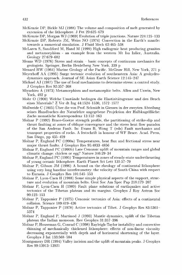
432 References

McKenzie DP, Bickle MJ (1988) The volume and composition of melt generated by extension of the lithosphere. J Pet 29:625-679

McKenzie DP, Morgan W J (1969) Evolution of triple junctions. Nature 224:125-133 McKenzie DP, Roberts JM, Weiss NO (1974) Convection in the Earth's mantle:

towards a numerical simulation. J Fluid Mech 62:465-538 McLaren S, Sandiford M, Hand M (1999) High radiogenic heat producing granites

and metamorphism - an example from the western Mt Isa Inlier, Australia. Geology 27:679-682

Means WD (1976) Stress and strain - basic concepts of continuum mechanics for geologists. Springer, Berlin Heidelberg New York, 339 p

Menard HW (1964) Marine Geology of the Pacific. McGraw Hill, New York, 271 p Meyerhoff AA (1995) Surge tectonic evolution of southeastern Asia: A geohydro­

dynamics approach. Journal of SE Asian Earth Science 12:145-247 Michael AJ (1987) The use of focal mechanisms to determine stress: a control study.

J Geophys Res 92:357-368 Miyashiro A (1973) Metamorphism and metamorphic belts. Allen and Unwin, New

York, 492 p Mohr 0 (1900) Welche Umstande bedingen die Elastizitatsgrenze und den Bruch

eines Materials? Z Ver dt Ing 44:1524-1530, 1572-1577 Mollweide C (1805) Uber die von Prof. Schmidt in Giessen in der zweyten Abteilung

seines Handbuches der Naturlehre angegebene Projektion der Halbkugelflache: Zachs monatliche Korrespondenz 13:152-163

Molnar P (1992) Brace-Goetze strength profile, the partitioning of strike-slip and thrust faulting at zones of oblique convergence and the stress heat flow paradox of the San Andreas Fault. In: Evans B, Wong T (eds) Fault mechanics and transport properties of rocks. A festschrift in honour of WF Brace. Acad. Press, San Diego, pp 435-459

Molnar P, England PC (1990a) Temperatures, heat flux and frictional stress near major thrust faults. J Geophys Res 95:4833-4856

Molnar P, England PC (1990b) Late Cenozoic uplift of mountain ranges and global climatic change: chicken or egg? Nature 346:29-34

Molnar P, England PC (1995) Temperatures in zones of steady-state underthrusting of young oceanic lithosphere. Earth Planet Sci Lett 131:57-70

Molnar P, Gibson JM (1996) A bound on the rheology of continental lithosphere using very long baseline interferometry: the velocity of South China with respect to Eurasia. J Geophys Res 101:545-553

Molnar P, Lyon-Caen H (1988) Some simple physical aspects of the support, struc­ture and evolution of mountain belts. Geol Soc Am Spec Pap 218:179-207

Molnar P, Lyon-Caen H (1989) Fault plane solutions of earthquakes and active tectonics of the Tibetan plateau and its margins. Geophys J Roy Astron Soc 99:123-153

Molnar P, Tapponier P (1975) Cenozoic tectonics of Asia: effects of a continental collision. Science 189:419-426

Molnar P, Tapponier P (1978) Active tectonics of Tibet. J Geophys Res 83:5361-5374

Molnar P, England P, Martinod J (1993) Mantle dynamics, uplift of the Tibetan plateau the Indian monsoon. Rev Geophys 31:357-396

Molnar P, Houseman G, Conrad C (1998) Rayleigh-Taylor instability and convective thinning of mechanically thickened lithosphere: effects of non-linear viscosity decreasing exponentially with depth and of horizontal shortening of the layer. Geophys J Int 133:568-584

Montgomery DR (1994) Valley incision and the uplift of mountain peaks. J Geophys Res 99:13913-13921

References 433

Morgan J (1968) Rises, trenches, great faults and crustal blocks. J Geophys Res 73:1959-1982

Morgan WJ (1971) Convection plumes in the lower mantle. Nature 230:42-42 Muller B, Reinecker J, Fuchs K (2000) The 2000 release of the world stress map

(available online at http://www-wsm.physik.uni-karlsruhe.de) Newman WI (1983) Nonlinear diffusion: Self-similarity and travelling waves. Pure

Appl Geophys 121:417-441 North GR, Cahalan RF, Coakley JA (1981) Energy balance climate models. Rev

Geophys Scace Phys 19:91-121 Oertel G (1996) Stress and deformation. A handbook on tensors in geology. Oxford

University Press, New York, 292 p Oilier CD (1985) Morphotectonics of continental margins with great escarpments.

In: Morrison M, Hack JT (eds) Tectonic geomorphology. Allan & Unwin, Boston, 390 p

Onsager L (1931) Reciprocal relations in irreversible processes. I Phys Rev 37:405-426

O'Rouke J (1993) Computational Geometry in C. Cambridge University Press, 346 p

Oxburgh ER (1980) Heat flow and magma genesis. In: Hargraves RB (eds) Physics of magmatic processes. Princeton University Press, Princeton NJ, pp 161-199

Oxburgh ER (1982) Heterogeneous lithospheric stretching in early history of oro­genic belts. In: Hsu K (ed) Mountain building processes. Academic Press, Lon­don, pp 85-94

Oxburgh ER, Turcotte DL (1974) Thermal gradients and regional metamorphism in overthrust terrains with special reference to the eastern Alps. Schweiz Mineral Petrograph Mitt 54:641-662

Parsons B, McKenzie D (1978) Mantle convection and the thermal structure of the plates. J Geophys Res 83:4485-4496

Parsons B, Richter FM (1980) A relationship between the driving force and the geoid anomaly associated with the mid-ocean ridges. Earth Planet Sci Lett 51:445-450

Parsons B, Sclater JG (1977) An analysis of the variation of ocean floor bathymetry with age. J Geophys Res 82:803-827

Passchier CW, Myers JS, Kroner A (1990) Field geology of high-grade gneiss ter­rains. Springer Verlag, Berlin 150p.

Pavlis TL (1986) The role of strain heating in the evolution of megathrusts. J Geo­phys Res 91:12407-12422

Peacock SM (1989) Numerical constraints on rates of metamorphism and fluid production fluid flux during regional metamorphism. Geol Soc Am Bull 101:476-485

Perry J (1895) On the age of the Earth. 51:224-227 & 341-342 & 582-585 Pfiffner OA, Lehner P, Heitzmann P, Mueller S, Steck A (eds) (1997) Deep structure

of the Swiss Alps. Results of NRP20. Birkhiiuser, Basel, 380 p Pierce KL, Coleman SM (1986) Effect of height and orientation (microclimate) on

geomorphic degradation rates and processes, late glacial terrace scarps in central Idaho. Geol Soc Am Bull 97:869-885

Pinter N, Brandon MT (1997) How erosion builds mountains. Scientific American, April 1997, pp 74-79

Pitman WC, Andrews JA (1985) Subsidence and thermal history of small pull­apart basins. In: Biddle K, Christie-Blick N (eds) Strike-slip deformation, basin formation and sedimentation. Spec Publ Soc Econ Palaeont Mineral 37:45-119

Platt JP (1990) Thrust mechanics in highly overpressured accretionary wedges. J Geophys Res 95:9025-9034

434 References

Platt .IP (1993a) Mechanics of oblique convergence . .I Geophys Res 98:16239-16256 Platt JP (1993b) Exhumation of high-pressure rocks: a review of concepts and

processes. Terra Nova 5:119-133 Platt JP, England PC (1994) Convective removal of lithosphere beneath mountain

belts: thermal and mechanical consequences. Am .I Sci 294:307 336 Pluijm B, Marshack S (1997) Earth structure - an introduction to structural geology

and tectonics. McGraw Hill, New York, 495 p Pollack HN, Chapman DS (1977) On the regional variation of heat flow, geotherms

and lithosphere thickness. Tectonophys 38:279-296 Powell R (1978) Equilibrium thermodynamics in petrology. Harper and Row, Lon­

don, 284 p Press WH, Flannery BP, Teukolsky SA, Vetterling WT (1989) Numerical receipes in

Pascal. The art of scientific computing. Cambridge University Press, Cambridge, 759 p

Price PH, Slack MR (1954) The effect of latent heat on numerical solutions of the heat flow equation. Br .I Appl Phys 3:379-384

Putnis A, McConnellJDC (1980) Principles of mineral behaviour. Geoscience Texts 1, Elsevier, New York, 257 p

Ramsay .IG, Huber M (1983) The techniques of modern structural geology, Strain analysis. Academic Press, San Diego, 1:1-300

Ramsay JG, Huber M (1987) The techniques of modern structural geology, Folds and fractures 2:301-700.

Ramsay .IG, Lisle RJ (2000) The techniques of modern structural geology, Applica­tions of continuum mechanics in structural geology. Academic Press, San Diego, 3:701-1061

Ranalli G (1987) Rheology of the Earth, 2nd edn. Chapman and Hall, London, 413 p

Ranalli G (1994) Nonlinear flexure and equivalent mechanical thickness of the litho­sphere. Tectonophys 240:107-114

Ratschbacher L, Frisch W, Linzer HG, Merle 0 (1991) Lateral extrusion in the Eastern Alps, part 2: structural analysis. Tectonics 10:245-256

Reece G (1986) Microcomputer modelling by finite differences. MacMillian. Bas-ingstoke UK, 125 p

Reiner M (1964) The Deborah number. Physics Today 17:62 Reiner M (1969) Deformation, strain and flow. HK Lewis, London, 360 p Richardson RM (1992) Ridge forces, absolute plate motions and the intra-plate

stress field . .I Geophys Res 97: 11 739-11 748 Ridley .I (1989) Vertical movement in orogenic belts and the timing of metamor­

phism relative to deformation. In: Daly .IS, Cliff RA, Yardley BWD (eds) Evo­lution of metamorphic belts. Geol Soc Lond Spec Pub 43: 103-115.

Ringwood (1988) Phase transformations and their bearing on the constitution and dynamics of the mantle. Geochim Cosmochim Acta 55:2083-2110

Robinson P (1990) The eye of the petrographer, the mind of the petrologist. Am Mineral 76:1781-1810

Robinson AH, Sale RD, Morrison JL, Muehrke PC (1984) Elements of Cartography, 5th edn. John Wiley and Sons, New York, 544 p

Roering JJ, Kirchner JW, Dietrich E (2001) Hillslope evolution by nonlinear, slope dependent transport: Steady state morphology and equilibrium adjustment time scales . .I Geophys Res 106:16499-16513

Roy RF, Decker ER, Blackwell DD, Birch F (1968) Heat flow in the United States . .I Geophys Res 73:5207-5221

References 435

Royden L, Keen CE (1980) Rifting processes and thermal evolution of the continen­tal margin of eastern Canada determined from subsidence curves. Earth Planet Sci Lett 51:343-361

Royden LH (1993a) The tectonic expression of slab pull at continental convergent boundaries. Tectonics 12:303-325

Royden LH (1993b) The steady-state thermal structure of eroding orogenic belts and accretionary prisms. J Geophys Res 98:4487-4507

Ruppel C (1995) Extensional processes in continental lithosphere. J Geophys Res 100:24187-24216

Rutland RWR (1965) Tectonic overpressures. In: Pitcher WS, Flinn GW (eds) Controls of metamorphism. Oliver and Boyd, New York, pp 119-139

Sabodini R, Lambeck K, Boschi E (eds) (1991) Glacial isostasy, sea level and mantle rheology. NATO ASI Series Serie C: Mathematical and physical sciences, 334 p

Sahagian DL, Holland SM (1993) On the thermomechanical evolution of continental lithosphere. J Geophys Res 98:8261-8274

Sambridge M, Braun J, Mcqueen H (1995) Geophysical parameterization and inter­polation of irregular data using natural neighbours. Geophys J Int 122:837-857

Sandiford M, Coblentz DD (1994) Plate-scale potential-energy distribution and the fragmentation of ageing plates. Earth Planet Sci Lett 126:143-159

Sandiford M, Powell, R (1990) Some isostatic and thermal consequences of the vertical strain geometry in convergent orogens. Earth and Planet Sci Lett 98:154-165

Sandiford M, Martin N, Zhou S, Fraser G (1991) Mechanical consequences of granite emplacement during high-T, low-P metamorphism and the origin of anticlock­wise PT paths. Earth Planet Sci Lett 107: 164-172

Sandiford M, Coblentz DD, Richardson RM (1995) Ridge-torques and continental collision in the Indo-Australian plate, Geology 23:653-656

Sandiford M, Hand M (1998a) Controls on the locus of intraplate deformation in central Australia. Earth Planet Sci Lett 162:97-110

Sandiford M, Hand M (1998b) Austalian Proterozoic high-temperature, low pres­sure metamorphism in the conductive limit. In: Treolar P, O'Brian P (eds.) What controls metamorphism. Gological Society of London special Publicaion 138: 103-114

Sandiford M, Hand M, McLaren S, (1998) High geothermal gradient metamorphism during thermal subsidence. Earth Planet Sci Lett 163:149-165

Sandiford M, McLaren S, Neumann N (2002) Long term thermal consequences of the redistribution of heat producing elements associated with large scale granitic complexes. J Metam Geol in press

Saunders AD, Tarney J, Kerr AC, Kent RW (1996) The formation and fate of large oceanic igneous provinces. Lithos 37:81-95

Sawyer DS (1985) Brittle failure in the upper mantle during extension of continental lithosphere. J Geophys Res 90:3021-3025

Schatz JF, Simmons G (1972) Thermal conductivity of Earth materials at high temperatures. J Geophys Res 77:6966-6983

Scheidegger AE (1961) Theoretical geomorphology. Prentice Hall, Englewood Cliffs, N. J., 333 P

Schmalholz SM, Podladchikov Y (1999) Buckling versus folding: Importance of Viscoelasticity. Geophys Res Lett 26:2641-2644

Scholz CH (1980) Shear heating and the state of stress on faults. J Geophys Res 85:6174-6184

Schumm SA (1956) The evolution of drainge basins and slopes in badlands at Perth Amboy, New Jersey. Bull Geol Soc Am 67:597-646

436 References

Schumm SA, Dumont JF, Holbrook JM (2000) Active Tectonics and Allivial Rivers. Cambridge University Press. 276p.

Sclater JG, Christie PA (1980) Continental stretching: an explanation of the post­mid Cretaceous subsidence of the central North Sea basin. J Geophys Res 85:3711-3739

Sclater JG, Jaupart C, Galson D (1980) The heat flow through oceanic and conti­nental crust and the heat loss of the Earth. Rev Geophys Space Phys 18:269-311

Selverstone J (1988) Evidence for east-west crustal extension in the Eastern Alps: implications for the unroofing history of the Tauern Window. Tectonics 7:87-105

Seth HC (1999) Flood basalts and large igneous provinces from deep mantle plumes: fact, fiction and fallacy. Tectonophysics 311:1-29

Shemenda AI (1994) Subduction: Insights from physical modelling. Kluwer Aca­demic Ser. Modern Approaches in Geophysics. Nethelands pp 215

Shreve RL (1967) Infinite topologically random networks. J Geol 75:178-186 Sleep NH (1971) Thermal effects of formation of Atlantic continental margins by

continental breakup. Geophys J Roy Astron Soc 24:325-350 Sleep NH (1979) A thermal constraint on the duration of folding with reference to

Acadian geology, New England (USA). J Geol 87:583-589 Sleep NJ (1992) Hotspot volcanism and mantle plumes. Annual Reviews of Earth

and Planetary Science 20:19-43 Smith GD (1985) Numerical solutions of partial differential equations: finite differ­

ence methods, 3rd edn. Oxford Applied Mathematics and Computing Science Series. Clarendon Press, Oxford, 337 p

Smoot NC (1997) Magma floods, micro plates and orthogonal intersections In Choi DR, Dickins JM (eds) New concepts in global tectonics Newsletter 5:8-13

Snyder JP (1987) Map projections - a working manual. USGS Prof Pap 1395, 383 p Snyder JP, Voxland RM (1989) An album of map projections: USGS Prof Pap 1453,

249 p Sonder LJ, Chamberlain CP (1992) Tectonic controls of metamorphic field gradi­

ents. Earth Planet Sci Lett 111:517-535 Sonder LJ, England P (1986) Vertical averages of rheology of the continental litho­

sphere: relation to "thin sheet"-parameters. Earth Planet Sci Lett 77:81-90 Spear FS (1993) Metamorphic phase equilibria and pressure-temperature-time

paths. Min Soc Am Monograph, Book Crafters, Chelsea, Michigan, 799 p Spear FS, Florence FP (1992) Thermobarometry in granulites: pitfalls and new

approaches. Precamb Res 55:209-241 Spear FS, Peacock SM (1989) Metamorphic pressure-temperature-time paths. Am

Geophys Union Short Course in Geology AGU press 7, 102 P Spiegel MR (1968) Mathematical handbook offormulas and tables. Schaums outline

series in mathematics. McGraw Hill, New York, 271 p Spiegelman M, McKenzie D (1987) Simple 2-D models for melt extraction at mid­

ocean ridges and island arcs. Earth Planet Sci Lett 83:137-152 Steckler MS, Watts AB (1978) Subsidence of Atlantik-type continental margin off

New York. Earth Planet Sci Lett 41:1-13 Steckler MS, Watts AB (1981) Subsidence history and tectonic evolution of Atlantic­

type continental margins. In: Scrutton, RA (ed) Dynamics of passive margins. Am Geophys U, Geodynamics Series 6:184-196

Stefan J (1891) Uber die Theorie der Eisbildung, insbesondere iiber die Eisbildung im Polarmeere. Annalen der Physik und Chemie 42:269-286

Stephansson 0 (1974) Stress-induced diffusion during folding. Tectonophys 22:233-251

Stockmal GS (1983) Modelling of large scale accretionary wedge deformation. J Geophys Res 88:8271-8287

References 437

Strahler AN (1964) Quantitative geomorphology of drainage basins and channel networks. In: Chow VT (ed) Handbook of applied hydrology, McGraw-Hill, New York Section 4-11

Strang G (1988) Linear algebra and its applications, 3rd edn. Harcourt Brace Jo­vanovich International Edition, 505 p

Stromgard KE (1973) Stress distribution during formation of boudinage and pres­sure shadows. Tectonophys 16:215-248

Stiiwe K (1991) Flexural constraints on the denudation of asymmetric mountain belts. J Geophys Res 96:10401-10408

Stiiwe K (1994) Process and age constraints for the formation of Ayers Rock / Aus­tralia - An example for two-dimensional mass diffusion with pinned boundaries. Z Geomorph 38:435-455

Stiiwe K (1995) The buffering effects of latent heat of fusion on the equilibration of partially melted metamorphic rocks. Tectonophys 248:39-51

Stiiwe K (1997) Effective bulk composition changes due to cooling: a model predict­ing complexities in retrograde reaction textures. Contrib Mineral Petrol 129:43-52

Stiiwe K (1998a) Heat sources for Eoalpine metamorphism in the Eastern Alps. A discussion. Tectonophys 287:251-269

Stiiwe K (1998b) Keyword: Diffusion. In: Marshall CP, Fairbridge RW (eds.) En­cyclopedia of Geochemistry. Chapman and Hall, London 133-140

Stiiwe K, Sandiford M (1994) On the contribution of deviatoric stresses to meta­morphic PT paths: an example appropriate to low-P, high-T metamorphism. J Met Geol 12:445-454

Stiiwe K, Sandiford M (1995) Mantle-lithospheric deformation and crustal meta­morphism with some speculations on the thermal and mechanical significance of the Tauern Event, Eastern Alps. Tectonophys 242:115-132

Stiiwe K, Sandiford M, Powell R (1993a) On the origin of repeated metamorphic­deformation events in low-P high-T terranes. Geology 21:829-832

Stiiwe K, Will TM, Zhou S (1993b) On the timing relationships between fluid production and metamorphism in metamorphic piles. Some implications for the origin of post-metamorphic gold mineralisation. Earth Planet Sci Lett 114:417-430

Stiiwe K, White L, Brown R (1994) The influence of eroding topography on steady­state isotherms. Application to fission track analysis. Earth Planet Sci Lett 124:63-74

Stiiwe K, Ehlers K (1997) Multiple metamorphic events at Broken Hill, Australia. Evidence from chloritoid-bearing parageneses in the Nine-Mile region. J Pet 38:1167-1186

Stiiwe K, Barr T (1998) On uplift and exhumation during convergence. Tectonics 17:80-88

Stiiwe K, Barr T (2000) On the relationship between surface uplift and gravitational extension. Tectonics 19:1056-1064

Stiiwe K, Hintermiiller M (2000) Topography and isotherms evisited: the influence of laterally migrating drainage divides. Earth Planet Sci Lett 184:287-303

Summerfield MA (1991) Global Geomorphology. Longman House, Burnt Mill, Eng­land, 537 p

Summerfield MA, Hutton NJ (1994) Natural controls of fluvial denudation rates in major world drainage basins. J Geophys Res 99:13871-13883

Suppe J (1981) Mechanics of mountain building and metamorphism in Taiwan. Mem Geol Soc China 4:67-89

Suppe J (1985) Principles of structural geology. Prentice Hall, Englewood Cliffs, N. J., 537 p

438 References

SuppeJ (1987) The active Taiwan mountain belt. In: Schaer JP, Rodgers .I (eds) The anatomy of mountain ranges. Princeton University Press, Princeton N. Y., pp 277-293

Talwani M, Worzel JL, Landisman M, (1959) Rapid gravity computations for two­dimensional bodies with application to the Mendocino Submarine fracture zone . .I Geophys Res 64:49-61

Tapponier P, Molnar P (1976) Slip-line field theory and large scale continental tectonics. Nature 264:319-324

Tapponier P, Peltzer G, Le Dain AY, Armijo R, Cobbolt P (1982) Propagating extrusion tectonics in Asia: new insights from simple experiments with plasticine. Geology 10:611-616

Tapponier P, Meyer B, Avouac JP Peltzer G, Gaudemer Y, Shulllnin G, Hongfa X, Kelun Y, Zhitai C, Shuahua C, Huagang D (1990) Active thrusting and folding in the Qilian Shan, and decoupling between upper crust and mantle in northeeastern Tibet. Earth Planet Sci Lett 97:382-403

Tarboton DG (1996) Fractal rivers networks, Horton's laws and Tokunga cyclicity . .I Hydrology 187:105-117

Taylor FB (1910) Bearing of the Tertiary mountain belt on the origin of the Earth's plan. Bull Geol Soc Am 21:179226

Telford WM, Geldart LP, Sheriff RE (1990) Applied geophysics, 2nd edn. Cam­bridge University Press, Cambridge, 770 p

Tex Eden (1963) A commentary on the correlation of metamorphism and defor­mation in space and time. Geol Mijnbouw 42:17176

Thompson AB, England PC (1984) Pressure-temperature-time paths of regional metamorphism Part II: some petrological constraints from mineral assemblages in metamorphic rocks . .I Pet 25:929-955

DuToit A (1937) Our wandering continents. Oliver and Boyd, Edinburgh, 366 p Tong H (1983) Threshold models in non-linear time series analysis. Lecture notes

in statistics, Springer, Berlin Heidelberg New York, 323 p Tucker GE, Slingerland R (1994) Erosional dynamics, flexural isostasy and long­

lived escarpments: A numerical modeling study . .I Geophys Res 99:1222912243 Tucker GE, Slingerland R (1996) Predicting sediment flux from fold and thrust

belts. Basin Res 8:329349 Turcotte DL (1979) Flexure. Advances in Geophys 21:51-86 Turcotte DL (1983) Mechanisms of crustal deformation. .I Geol Soc London

140:701-724 Turcotte DL (1997) Fractals and chaos in geology and geophysics, 2nd edn. Cam­

bridge University Press, Cambridge, 398 p Turcotte DL, Oxburgh ER (1973) Mid-plate tectonics. Nature, 244:337339 Turcotte DL, Schubert G (1982) Geodynamics. Applications of continuum physics

to geological problems. John Wiley and Sons, New York, 450 p Turcotte DL, Haxby WF, Ockendon JR (1977) Lithospheric instabilities. In: Tal­

wani M, Pitman III WC (eds) Island arcs, deep sea trenches and back-arc basins. Am Geophys U, Maurice Ewing Series Washington 1:63-69

Turner S, Arnaud N, Liu .I, Rogers N, Hawkesworth C, Harris N, Kelley S, Van Calsteren P, Deng W (1995) Post collision shoshonitic volcanism in the Tibetan plateau: Implications for convective thinning of the lithosphere and the source of ocean island basalts . .I Pet 37:45-71

Twiss RJ, Moores EM (1992) Structural geology. Freeman and Company, New York 532 p

Vilotte .1P, Daignieres M, Madariaga R (1982) Numerical modeling of intraplate deformation: simple mechanical models of continental collision . .1 Geophys Res 87:10709-10728

References 439

Vine F, Mathews D (1963) Magnetic anomalies over oceanic ridges, Nature 199:947~ 949

Voorhoeve H, Houseman G (1988) The thermal evolution of lithosphere extending on a low angle detachment zone. Basin Res 1:1~9

Waschbusch PJ, Royden LH (1992) Episodicity in for deep basins. Geology 20:915~ 918

Watts AB, Ryan WBF (1976) Flexure of the lithosphere and continental margin basins. Tectonophys 36: 24~44

Watts AB (1976) Gravity and bachymetry in the central Pacific ocean. J Geophys Res 81:1533~1553

Wees JD, Jong KC, Cloetingh S (1992) Two dimensional P-T-t-modelling and the dynamics of extension and inversion in the Beltic Zone (SE Spain). Tectonophys 302:305~324

Wegener A (1912a) Die Entstehung der Kontinente. Petermanns Geographische Mitteilungen 9127:185~308

Wegener A (1912b) Die Entstehung der Kontinente. Geol Rundsch 3:276~292 Wegener A (1915) Die Entstehung der Kontinente und Ozeane. Sammlung Vieweg

23, 94 p Weijermars R (1997) Principles of rock mechanics. Alboran Science Publishing,

Amsterdam, 359 p Wells PRA (1980) Thermal models for the magmatic accretion and subsequent

metamorphism of continental crust. Earth Planet Sci Lett 46:253~265 Wernicke B (1985) Uniform sense normal simple shear ofthe continental lithosphere.

Canad J Earth Sci 22:108~125 Wessel P, Smith WHF (1995) New version of the generic mapping tool released,

EOS, Amer. Geophys U 76, 329 Wheeler J (1991) Strucutral evolution of a subducted continental sliver: the north­

ern Dora Maira massif, Italian Alps. J Geol Soc London 148:1103~1113 White R, McKenzie D (1989) Magmatism at rift zones: the generation of volcanic

continental margins and flood basalts. J Geophys Res 94:7685~7729 Wickham SM (1987) The segregation and emplacement of granitic magmas. J Geol

Soc London 144:281~297 White RW, Powell R, Holland TJB (2001) Calculation of partial melting equilib­

ria in the system Na20-CaO-K20-FeO-MgO-Ab03-Si02-H20. J Metam Geol 19:139~153

Wignall PB (2001) Large igneous provinces and mass extinctions. Earth Science Reviews 53:1~33

Wilde M, Stock J (1997) Compression directions in southern California (from Santa Barbara to Los Angeles basin) obtained from borehole breakouts. J Geophys Res 102:4969~4983

Will TM (1998) Phase equilibrian in metamorphic rocks. Lecture notes in Earth Science, Springer 315 pp.

Willet S (1992) Dynamic and kinematic growth and change of a Coulomb wedge. In: McClay KR (ed) Thrust tectonics. Chapman and Hall, pp 19~31

Willet S, Beaumont C, Fullsack P (1993) Mechanical model for the tectonics of doubly vergent compressional orogens. Geology 21:371~374

Willgoose G, Bras RL, Rodriguez-Iturbe I (1991) Results from a new model ofriver basin evolution. Earth Surface Processes and Landforms 16:237~254

Wilson JT (1963) A possible origin of the Hawaiian islands. Canad J of Physics 41:863~868

Wilson JT (1972) Continents adrift. Readings from Scientific American Freeman WH and Company, San Francisco, 172 p

440 References

Wilson M (1993) Plate-moving mechanisms: constraints and controversies. J Geol Soc London 150:923-926

Winter J (2001) Introduction to igneous and metamorphic petrology. Prentice Hall, 699 pp.

Wintsch RP, Andrews MS (1988) Deformation induced growth of sillimanite: "stress"minerals revisited. J Geol 96:143-161

Won IJ, Bevis M (1987) Computing the gravitational and magnetic anomalies due to a polygon: algorithms and Fortram subroutines. Geophys 52:232-238

Xu G, Will TM, Powell R (1994) A calculated petrogenetic grid for the system K 2-

FeO-MgO-Ab03-Si02-H20, with particular refeence to contact metamorphosed pelites. J Metam Geol 12:99-119

Yale LB, Carpenter SJ (1998) Large igeneous provinces and giant dike swarms; proxies for supercontinent cyclicity and mantle convection. Earth Planet Sci Lett 163:109-122

Yardley BWD (1989) An introduction to metamorphic petrology. Longman Harlow UK, 248 p

Zen E-an (1966) Construction of pressure-temperature diagrams for multicompo­nent systems after the method of Schreinemakers: a geometric approach. USGS Bull 1225, 56 p

Zhou S, Sandiford M (1992) On the stability of isostatically compensated mountain belts. J Geophys Res 97:14207-14221

Zhou S, Stiiwe K (1994) Modeling of dynamic uplift, denudation rates thermome­chanical consequences of erosion in isostatically compensated mountain belts. J Geophys Res 99: 13923-13939

Ziegler PA (1992) Plate tectonics, plate moving mechanisms and rifting. Tectono­phys 215:9-34

Ziegler PA (1993) Plate-moving mechanisms: their relative importance. J Geol Soc London 150:927-940

Zill DG (1986) A first course in differential equations with applications (3rd edition). PWS-Kent Publishing, Boston, 520 p

Zoback ML (1992) First- and second-order patterns of stress in the lithosphere: the world stress map project. J Geophys Res 97:11703-11728

Zoback ML, Haimson BC (1983) Hydraulic fracturing stress measurements US Nat Comm for Rock Mechanics, Nat Acad Press, Washington D. C., 270 p

Index

A

Acceleration - angular, 23 - gravitational, 24, 70 - of plates, 24 Accretionary wedge, 98, 231, 294 Accuracy - definition, 5 -- numerical, 357, 359 Acoustic energy, 63 Activation - energy, 215, 325 - volume, 325 AD I-method, 361 Adiabatic - compressibility, 69 - gradient, 70

melting, 32 - processes, 69 Advection, 74 Africa - lithosphere, 33 - rift, 39 Airy, 153 Altiplano, 285 Amontons law, 210 Analytical solution, 352 Andersons theory, 210 Angle of friction, 210 Angular - acceleration, 23 - momentum, 25 - velocity, 23 - velocity of plates, 38 Arc - island, 99 - magmatic, 99 Argand number, 291 Arrhenius relationship, 215, 325

Asthenosphere - definition, 34 Atmosphere C02, 311 Australia, 166, 265 Ayers rock, 9

B

Back stripping, 259 Back thrust, 288 Back-arc basin, 40, 240, 255 Barometry, 327 Barrier reef, 166 Basin - back-arc, 40, 240 - fore-arc, 255 - foreland, 40, 255 - intra-continental, 255 - McKenzie model, 261 - molasse, 161 - origin, 252 - types, 254 Bending - of continental plates, 161 - of oceanic plates, 160 Benioff zone, 40, 100 Bifurcation ratio, 184 Black smokers, 40 Boundary condition - at infinity, 95, 101 -- definition, 354 - mechanical, 231

orogenic, 26 - thermal, 110 Boundary layer - mechanical, 34

thermal, 34, 302 Brace-Goetze lithosphere, 220 Brittle - deformation, 208

442

- ductile transition, 210, 219, 310 Bulk modulus, 208 Buoyancy force, 233, 281 Butterfly effect, 317 Byerlees law, 210

c

Chaos, 187, 312 Cheese tectonics, 19 Chemical boundary layer, 34 Clapeyron curve, 99 Coast line - fractal dimension, 189 Cohesion, 208 Collision

momentum, 244 - of continental plates, 40 - of oceanic plates, 41 - of plates generally, 40 Compaction, 256 Compensation depth, 151, 233 Complementary error function, 57 Compressibility

adiabatic, 69 Conductivity - changes, 52 - thermal, 49 Confidence interval, 376 Constitutive relationship, 205 Contact metamorphism, 52, 76, 104,

305, 333 Continent

mean elevation, 136 Continental - collision, 269

elevation, 390 - geotherm, 83 - lithosphere, 36 Convection, 74 Convergence - of plates, 41, 282 Cooling - of earth, 54 - of half space, 95 - of oceanic lithosphere, 95 Cooling rate, 105 Coordinates

cartesian, 21 - cylindrical, 54 - polar, 21 - reference frame, 136

spherical, 54

Core - of earth, 32 Corner flow model, 298 COST-drilling program, 252 Coulomb criterion, 208, 295 Crank-Nicolson, 360 Crust - continental, 36 - oceanic, 95, 238 Crystalli'lation - heat, 112 - of dikes, 112 Curvature - definition, 350

D

Deborah number, 292 Deccan, 237, 300 Declination, 22 Deformation

laws, 205 - maps, 215 - permanent, 208 Degradation - of scarps, 174 Delamination, 302 Density

of the crust, 34, 52, 155

Index

of the mantle lithosphere, 34, 155 Derivatives - order, 351 Dextral, 212 Differential - partial, 351 - total, 351 Differential equation, 349 - analytical solution, 353 - method of solution, 369, 372 - numerical solution, 353 - order, 351 - ordinary, 352 - partial, 352 Differential stress, 68, 200 Diffusion - cation, 330 - equation, 50 - mass, 171 - nonlinear, 173 - numerical, 75, 362 - radial, 54 Diffusion age, 179 Diffusivity, 215

Index

erosional, 172 - thermal, 51 Dike - swarms, 108 - thermal evolution, 103 Dimension - dimensionless, 10 - one-dimensional, 12 - spatial, 6 - three-dimensional, 9 - two-dimensional, 11 - units, 23 - zero-dimensional, 9 Dislocation energy, 63 Displacement, 280 Dissipative heat production, 63 Distribution - Gaussian, 375 - normal, 375 Divergence - definition, 368 Dorn law, 216 Driving force - plate tectonic, 226, 230, 280 Ductile deformation, 202 Ductile vs viscous, 206 Dynamic - collision, 279 - extension, 267 Dynamics - on a sphere, 24

E

Earth - age of, 54 - core, 32

layer structure of, 31 - radius, 134 - shape, 134

total heat loss, 81 Earthquake, 212 - distribution, 228 Eclogite, 308 Elastic - bulge, 161 - thickness, 161 Elasticity - law, 206 - of continents, 166 - of oceanic plates, 164 Elevation - of mountain belts, 154

Ellipticity, 135 Elongation, 64 - definition, 196 endogenic process, 167 Endothermic -- reaction, 71 Energy - acoustic, 63 - activation, 215 - equilibrium, 49 - Gibbs, 328 - kinetic, 245 - potential, 63, 265 Equator - radius, 135, 387 Equilibrium - coefficient, 328 - force, 204 - isostatic, 150 - steady state, 56, 83, 146, 186, 297 - thermodynamic, 328 - transient, 83 Erosion model, 146, 168, 169 Error function, 56, 383

derivative of, 97 Escarpment, 161 Euler - reference frame, 76 Eulerian - description, 75 - reference frame, 78, 136, 167 Exhumation, 140 - mechanism, 307 exogenic process, 167 Exothermic - reaction, 71 Expansion - thermal, 69, 154 Explicit methods, 359 Extension - active, 251, 266, 299 - brittle, 210

continental, 138 - force, 281 -- lateral, 289 - pasive, 299 - passive, 251, 266, 267 - rheology change, 221

self limiting, 267 - two-dimensional, 265 Extrusion - lateral, 289, 294 - vertical, 307

443

444

F

Fault - orientation, 211 - plane solution, 212 - temperatures, 125, 140 - transform, 42 Feedback, 311 Ficks law, 48, 173 Finite - difference method, 131, 354 - element method, 353 Finite difference method - stability, 358 Flexural - parameter, 165 - rigidity, 161 Flexure - of plates, 159 Flood basalt, 239 Flood basalts, 298 Flow - of heat, 48 - of mass, 48 - viscous, 215 - volumetric, 48 Flow law, 205 Fluid - flow, 80, 100 - heat transport, 79 - Newtonian, 216 - pressure, 210 Fold and thrust belt, 294 Folding - of isotherms, 118 - rate, 118 Force, 196 - applied to oceanic plates, 237 - driving plates, 232 - extension, 281 - transmission, 230 - units, 24 Force balance - extension, 267 - in orogens, 283 Fore-arc basin, 40, 240, 255 Foreland basin, 240, 255 Fourier - cell number, 357 - first law, 48, 172, 324 - second law, 49 - series, 370

Fractal, 312 - geometrical, 187 - statistical, 188 Friction coefficient, 208 Friction heat, 63, 125, 322, 341 Fusion heat, 71

G

Gas constant, 325 Gaussian distribution, 375 Geobarometer, 199 Geobarometry, 327 Geochrononology, 326 Geoid - anomaly, 135, 234 - definition, 134 Geometry - on a sphere, 21 Geosyncline, 43 Geotherm - continental, 83 - definition, 82 - oceanic, 95 Geothermometry, 327 Gondwana, 15 GPS, 212 Graded rivers, 184 Gradient, 54 - definition, 368 Granitic weathering, 175 Gravitational - acceleration, 70, 159, 204, 323 - constant, 5 - stress, 233 Great barrier reef, 166 Great circle, 22 Great Escarpment, 265 Great escarpment, 161, 171 Greenwich, 22

H

Index

Half-space cooling model, 95, 103, 158 Hawaii, 165, 193 Heat - capacity, 50 - conductivity, 49 - content, 72 - content of intrusions, 116 - content of terrains, 116 - dissipative, 125 - friction, 341

Index

- of fusion, 71 -- refraction, 52 Heat flow - at the surface, 93, 226 - definition, 49 - from mantle, 86 - from the manlte, 130 - mantle, 273, 276 - oceanic, 97 - surface, 273 - two-dimensional, 54, 109, 121 - unit, 49 Heat production - by friction, 63 - by radioactivity, 61, 85 - by reaction, 70 - distribution, 87 Heat transfer - by active transport, 74 - by diffusion, 48 - types of, 47 High pressure metamorphism, 307 Himalaya, 53, 182, 245, 314 Histogram, 375 Hooks law, 207 Hydrostatic isostasy, 150 Hydrostatic pressure, 151, 181, 204

I

Iceland, 239 Implicit methods, 359 Inclination, 22 Incompressibility, 207 Indenter, 293, 307 Initial condition - definition, 354 Interferometry, 212 Intra-continental basins, 255 Intrusion - cooling of, 105 - heat content, 116 - spherical, 109 - thermal evolution, 101 Invariant - tensor, 199 Island arc, 41, 99, 294 Isograds - stretching, 126 - telescoping, 126 Isostasy, 151 - Airy, 153 - equilibration rate, 150

- flexural, 159 - hydrostatic, 150 - Pratt, 153 Isotherms -- around faults, 125 - folding of, 118 - topography, 121

J

Julia set, 312

K

Karoo, 237 Kelvin model, 54 Kinematics - on a sphere, 23 - vertical, 140 Kinetic - energy, 245 Kinetics -- of reaction, 185 Kochs snow flake, 188 Kurtosis, 376

L

La Place equation, 56 Lagrangian - coordinates, 353 - description, 75, 178 - reference frame, 136 Landscape model, 186 Landslide, 187 Large igneous provinces, 298 Latent heat - of evaporation, 71 - of fusion, 71, 113 Laurasia, 15 Layers of earth, 32 Least squares, 373 Liquidus, 72 Lithosphere - definition, 34 - mantle part, 34, 89 - mechanical definition, 230 - subdivision, 33 - temperature at base, 34 - thermal definition, 81 - types of, 36 Lithosphere thickness - elastic, 154, 222

445

446

- mechanical, 35 - thermal, 35 Lithostatic pressure, 204 Load - external, 163, 222 - internal, 163, 222 Longitudinal wave, 212 Lorentz attractor, 312 Loxodrome, 22 LPHT-terrains, 304 Luzon, 294

M

Main Central Thrust, 53 Mantle - definition, 32 - density, 155 - discontinuity, 240 - heat flow, 86, 272 - lithosphere, 34, 89, 95, 220 - plume, 239, 243 - viscosity, 150, 151 - wedge convection, 100 Mantle lithosphere, 154, 251 Mantle plume, 267 Mantle plumes, 298 Map projection, 26 - azimuthal, 29 - conical, 29 - cylindrical, 28 - true to angle, 27 - true to area, 27 Mariana trench, 15 Mass extinctions, 301 Mass flux, 48, 172 Matrix, 198 Mean - depth, 136 - elevation, 136, 390 - surface heat flow, 390 Mercator projection, 28 Meridian, 22 Metamorphic field gradient - definition, 339 Metamorphic geotherm - definition, 340 Metamorphic gradient - contact, 107, 343 - inverted, 126 - regional, 275, 338 Metamorphism - Barrovian, 276, 304

Index

- contact, 52, 305 - high pressure, 307 - LPHT,304 - regional, 270, 275, 340 - space-time relations, 340 - space-time relationship, 275 Michigan basin, 266 Mid-oceanic ridge, 16, 95, 157, 237 - manometer, 34, 156 Model - concept, 2 - requirements, 6 Moho - definition, 32 - heat flow, 130 - temperature, 93 Mohr-Colulomb criterion, 208 Molasse, 161 Moment - of inertia, 25 Momentum, 24, 25, 244 - angular, 25 Mt Blanc, 10 Mt Everest, 10

N

Nabla operator, 54 Network law, 183 New degrees, 22 Newton - units, 24 Newtonian fluid, 215 Nodal plane, 214 Normal fault, 211 Normal stress, 197 Normalize, 10 Nucleation rate, 324 Numerical - diffusion, 75, 362 - solution, 352

o

Obduction, 40 Ocean - mean depth, 136 Oceanic - CHABLIS model, 98 - cooling, 95 - geotherms, 93 - water depth, 157, 390

Index

Olivine, 32, 66, 99, 217, 224, 239, 268, 386

Orogenic force balance, 283

p

P-wave, 212 Paired metamorphic belt, 99 Palaeopiezometry, 327 Palaeostress, 212 Pannonian basin, 266 Parametric diagram, 106, 322 Passive margin, 161, 254 Peclet number, 80 Periodic problems, 117 Petrology, 323 Phase ~ transition, 71 Phase rule, 328 Piezometry, 196 Piezothermal array, 342 Ping-pong ball model, 20 Plane strain, 11, 292 Plate ~ graveyards, 241 ~ tectonic driving force , 230 ~ tectonics, 15 Plate boundary ~ convergent, 40, 269 ~ diffuse, 19 ~ divergent, 39 ~ passive, 39, 254, 268 ~ transform, 41 Plume ~ mantle, 239 Poisson constant, 161, 207 Porosity, 80, 256 Post orogenic collapse, 293 Potential ~ surface, 8, 368 Potential energy, 63, 232, 265 ~ continents, 241 Power law ~ definition, 216 ~ exponent, 216 Pratt, 153 Pre-exponent constant, 215 Precision ~ definition, 5 Pressure, 345 ~ chemical, 199 ~ hydrostatic, 204 ~ mechanical, 199

~ tectonic, 204, 308 Pressure-depth relationship, 323 Projection ~ of maps, 26 Pseudotachylite, 64 PT-path, 321 ~ anticlockwise, 334 ~ interpretation, 276 ~ parts of, 326 ~ shape, 334 Pure shear, 143 Pythagoras, 367

Q

Quadratic equation, 383

R

Radioactive heat, 61 Radius ~ of earth, 134 Reaction ~ endotherm, 71 ~ exotherm, 71 ~ rate, 324 Reaction heat ~ dehydration, 71 ~ melting, 71 Red Sea, 43, 265 Reference frame, 136 ~ Eulerian, 78 ~ Lagrangian, 136 Reference levels, 133 Refraction ~ of heat, 52 Retro-arc foreland basin, 255 Rheology ~ definition, 218 ~ of continents, 218 ~ of oceans, 226 ~ olivine, 222 ~ quartz, 222 Rhumb line, 22 Ridge push, 237 Rift, 39 ~ basin, 254 Rifted margin sequence, 298 Rifting, 299 Roll back, 240 Rotation pole, 23

447

448

s

Scalar - definition, 365 Scarp - degradation, 174 Schmidt net, 27, 213 Sea level - mean, 136 Sea mount, 160 Sedimentary basin - origin, 252 Seismicity, 228 Shear - pure, 265 - simple, 143, 265 - strength, 68 - stress, 197 Shear strength - definition, 202 Shear zone, 66, 143, 265, 289 Shields, 142, 304 - continental, 89 Simple shear, 143 Skewness, 376 Skin depth, 89 Slab breakoff, 240 Slab pull, 239 Slope - of a function, 349 Snowball earth, 311 Solar system, 4 Solidus, 72 Solution - analytical, 353 - numerical, 352 South Georgia, 240 Specific heat, 50, 52 Speed - definition, 23 Sphere - latitude, 21 - longitude, 21 - meridian, 22 Spheroid, 135 Stability - numerical, 357, 359 Stable geotherm, 83 Standard deviation, 376 Steady state - equilibrium, 56 - geotherm, 83 - surface elevation, 146

Stefan problem, 112 Strain - definition, 196, 207 - hardening, 201 - longitudinal, 64 - plane, 11, 289, 292 - rate, 12 Strength - continents, 223 - definition, 202 - integrated, 225 - mean, 64, 285 - of the continents, 219 - of the oceans, 227 Stress - deviatoric, 63, 200 - differential, 68, 200 - mean, 199 - principal, 198 - shear, 197 - tensor, 196 Stress profile - quantitative, 223 Stretch - definition, 196 Strike slip fault, 211, 214 Subduction zone, 40, 98 - accretionary wedge, 294 - force balance, 40 - geometry, 8 - isotherms, 98 - roll back, 240 - shape, 160, 164 - slab break off, 240 Subsidence - analysis, 255 - isostatic, 253 - mechanisms, 253 - tectonic, 252 - total, 252 Surface - heat flow, 93, 97, 226, 273, 313 Surface elevation, 154 - evolution, 146 Surface heat flow - mean, 390

T

Taiwan, 294 Tectonic - driving force, 281, 283 - pressure, 205, 308

Index

Index

Temperature - absolute, 326 - dimensionless, 10 - fluctuations, 117 - steps, 102 Tensor - calculation, 366 - stress, 197 Thermal - boundary layer, 34, 59, 302 - conductivity, 49 - expansion, 69, 154 Thermodynamic - degree of freedom, 328 - equilibrium, 328 Thermomechanics, 279 Thermometry, 327 Thickness - elastic, 163 - of elastic lithosphere, 161 - of mechanical lithosphere, 35 - of thermal lithosphere, 35, 81 Thin sheet approximation, 12, 289 Thomas algorithm, 360 Threshold, 187 - mechanism, 316 Thrust, 211 Tien Shan, 231 Time constant - diffusive, 325 - thermal, 57 Topography - dynamic, 159 Torque, 24, 237 Traction - definition, 197 Transform - basin, 254 - plate boundary, 41 Trench, 164 - suction, 239 Triple junction, 42 Two-dimensional - deformation, 137 - force equilibrium, 279

u

Under plating, 76 Units - in this book, 385 - mistakes with, 23 Uplift, 140

- of rocks, 141 - surface, 146 UTM projection, 28

v

Variance, 376 Vector - calculation, 366 - definition, 366 Velocity - angular, 23 - definition, 23 Vertical - kinematics, 140 Viscosity - dynamic, 215 - effective, 216 - kinematic, 215 - mantle, 150 Volcano - shape, 181

w

Wegener, 15 Wilson cycle, 42, 265 Wulff net, 27

y

Young's modulus, 161, 207

449