a mathematical model for the transpiration and ... · a mathematical model for the transpiration...
TRANSCRIPT
A Mathematical Model for theTranspiration and Assimilation of
Early Devonian Land Plants with
Axially Symmetric Telomes
Diplomarbeit
an der
Geowissenschaftlichen Fakultat
der
Eberhard-Karls-Universitat Tubingen
vorgelegt von
Wilfried Konrad aus Zaisenhausen bei Bretten
Tubingen Marz 2002

Ich versichere, daß ich bei der Anfertigung der vorliegenden Arbeit lediglich die angegebenen Hilfs-
mittel benutzt habe.
Tubingen, den 8. Marz 2002
Abstract
Early terrestrial ancestors of the land flora are characterized by a simple, axially symmetric habit
and evolved in an atmosphere with much higher carbon dioxide concentrations than today.
In order to gain information about the ecophysiological interrelationships of these plants we intro-
duce a model which encompasses gas diffusion within plants, photosynthesis and gaseous exchanges
between plants and the atmosphere. Based on the mechanics of gas diffusion inside a porous medium
and on a well-established quantitative description of photosynthesis, the model allows for the math-
ematical simulation of the local gas fluxes through the various tissue layers of a plant axis.
Parameters entering the model consist of, (i) kinetical properties of the assimilation process and
other physiological parameters (which have to be taken from extant plants), (ii) physical constants of
nature, and, (iii) anatomical parameters which can be obtained from well-preserved fossil specimens.
The model system is applied to two Early Devonian land plants, Aglaophyton major and Rhy-
nia gwynne-vaughanii. The results demonstrate that, under an Early Devonian carbon dioxide
concentration, both Aglaophyton major and Rhynia gwynne-vaughanii show extremely low transpi-
ration rates and low, but probably sufficiently high assimilation rates. Variation of the atmospheric
carbon dioxide concentration shows that the assimilation of Aglaophyton major and Rhynia gwynne-
vaughanii is fully saturated even if the carbon dioxide content is decreased to about two thirds and
one third of the initial value, respectively. This result indicates that both plants were probably
able to exist under a wide range of atmospheric carbon dioxide concentrations.
Further applications of the model system to axially symmetric plants include the (sub-)systematic
variation of the physiological and anatomical parameters “defining” these plants and the responses
of the assimilation and transpiration rates to these variations. Examples are given, how such
sensitivity studies can be used to identify ecophysiological optima and to understand functional
morphological aspects of (extinct) land plants.
To the three therapsideswhich came from beyond the palaeozoic borderlineand kept me good company during my studies.

Contents
1. Introduction . . . . . . . . . . . . . . . . . . . . . . . . . . . . . . . . . . . . . . . . . . . . . . . . . . . . . . . . . . . . . . . . . . . . . . . . . . . . . 1
2. Characteristic Features of Rhyniophytic Plants . . . . . . . . . . . . . . . . . . . . . . . . . . . . . . . . . . 3
3. The Mathematical Model . . . . . . . . . . . . . . . . . . . . . . . . . . . . . . . . . . . . . . . . . . . . . . . . . . . . . . . . . . . . 8
3.1 The Process of Diffusion . . . . . . . . . . . . . . . . . . . . . . . . . . . . . . . . . . . . . . . . . . . . . . . . . . . . . . . . . . . . . . . . . . 8
3.2 Diffusion in Rhyniophytic Plants — Problems and Further Proceeding . . . . . . . . . . . . . . . . . . . . 10
3.3 Approximations . . . . . . . . . . . . . . . . . . . . . . . . . . . . . . . . . . . . . . . . . . . . . . . . . . . . . . . . . . . . . . . . . . . . . . . . . . 10
3.3.1 The porous medium approach . . . . . . . . . . . . . . . . . . . . . . . . . . . . . . . . . . . . . . . . . . . . . . . . . . . . . . . . 10
3.3.2 Translatorial symmetry . . . . . . . . . . . . . . . . . . . . . . . . . . . . . . . . . . . . . . . . . . . . . . . . . . . . . . . . . . . . . . 14
3.3.3 Stationarity . . . . . . . . . . . . . . . . . . . . . . . . . . . . . . . . . . . . . . . . . . . . . . . . . . . . . . . . . . . . . . . . . . . . . . . . . . 14
3.3.4 Constancy of effective conductance S . . . . . . . . . . . . . . . . . . . . . . . . . . . . . . . . . . . . . . . . . . . . . . . . . 15
3.4 Photosynthesis . . . . . . . . . . . . . . . . . . . . . . . . . . . . . . . . . . . . . . . . . . . . . . . . . . . . . . . . . . . . . . . . . . . . . . . . . . . 17
3.4.1 The Model of Photosynthesis — General Remarks . . . . . . . . . . . . . . . . . . . . . . . . . . . . . . . . . . . . 17
3.4.2 Connection between Diffusion and Photosynthesis . . . . . . . . . . . . . . . . . . . . . . . . . . . . . . . . . . . . 25
3.4.3 Linear Approximation of the Model of Photosynthesis . . . . . . . . . . . . . . . . . . . . . . . . . . . . . . . . 28
3.5 The solution procedure . . . . . . . . . . . . . . . . . . . . . . . . . . . . . . . . . . . . . . . . . . . . . . . . . . . . . . . . . . . . . . . . . . 32
4. Application of the Model to the Anatomies of Aglaophyton and Rhynia . . . . . . 41
4.1 Boundary layer . . . . . . . . . . . . . . . . . . . . . . . . . . . . . . . . . . . . . . . . . . . . . . . . . . . . . . . . . . . . . . . . . . . . . . . . . . 41
4.2 Stomatal layer . . . . . . . . . . . . . . . . . . . . . . . . . . . . . . . . . . . . . . . . . . . . . . . . . . . . . . . . . . . . . . . . . . . . . . . . . . . 42
4.3 Hypodermal channels . . . . . . . . . . . . . . . . . . . . . . . . . . . . . . . . . . . . . . . . . . . . . . . . . . . . . . . . . . . . . . . . . . . . 43
4.4 Assimilation layer . . . . . . . . . . . . . . . . . . . . . . . . . . . . . . . . . . . . . . . . . . . . . . . . . . . . . . . . . . . . . . . . . . . . . . . . 44
5. Plant Material and Methods for Obtaining Relevant Anatomical Data . . . . 47
5.1 General Approach . . . . . . . . . . . . . . . . . . . . . . . . . . . . . . . . . . . . . . . . . . . . . . . . . . . . . . . . . . . . . . . . . . . . . . . 47
5.2 Numerical Values . . . . . . . . . . . . . . . . . . . . . . . . . . . . . . . . . . . . . . . . . . . . . . . . . . . . . . . . . . . . . . . . . . . . . . . . 48
Table 1 — Anatomical Properties . . . . . . . . . . . . . . . . . . . . . . . . . . . . . . . . . . . . . . . . . . . . . . . . . . . . . . . . . 54
Table 2 — Environmental Parameters . . . . . . . . . . . . . . . . . . . . . . . . . . . . . . . . . . . . . . . . . . . . . . . . . . . . . 55
Table 3 — Biochemical and Physiological Parameters . . . . . . . . . . . . . . . . . . . . . . . . . . . . . . . . . . . . . . 55
6. Results . . . . . . . . . . . . . . . . . . . . . . . . . . . . . . . . . . . . . . . . . . . . . . . . . . . . . . . . . . . . . . . . . . . . . . . . . . . . . . . . . . 56
6.1 Local Fluxes and Local Concentrations of Carbon Dioxide and Water Vapour . . . . . . . . . . . . . 58
6.2 Transpiration and Assimilation Rates and their Dependance on Environmental Conditions 59
6.3 The Water Use Efficiency and its Dependance on Atmospheric Conditions . . . . . . . . . . . . . . . . 61
6.4 Dependance of Water Use Efficiency, Transpiration and Assimilation Rates on Plant Anatomy 62
6.5 Dependance of the Assimilation Rate on the Liquid Phase Conductance of Carbon Dioxide 64
6.6 Dependance of the Assimilation Rate on the Specificity Factor for Rubisco . . . . . . . . . . . . . . . . 65

6.7 Dependance of the Assimilation Rate on the Efficiency of Light Conversion . . . . . . . . . . . . . . . 65
6.8 Dependance of the Assimilation Rate on Vmax and Jmax . . . . . . . . . . . . . . . . . . . . . . . . . . . . . . . . . . 66
7. Discussion . . . . . . . . . . . . . . . . . . . . . . . . . . . . . . . . . . . . . . . . . . . . . . . . . . . . . . . . . . . . . . . . . . . . . . . . . . . . . . 67
7.1 Local Fluxes and Local Concentrations of Carbon Dioxide and Water Vapour . . . . . . . . . . . . . 67
7.2 Transpiration and Assimilation Rates and their Dependance on Environmental Conditions 68
7.3 The Water Use Efficiency and its Dependance on Atmospheric Conditions . . . . . . . . . . . . . . . . 70
7.4 Dependance of Water Use Efficiency, Transpiration and Assimilation Rates on Plant Anatomy 72
7.5 Dependance of the Assimilation Rate on the Liquid Phase Conductance of Carbon Dioxide 73
7.6 Dependance of the Assimilation Rate on the Specificity Factor for Rubisco . . . . . . . . . . . . . . . . 73
7.7 Dependance of the Assimilation Rate on the Efficiency of Light Conversion . . . . . . . . . . . . . . . 74
7.8 Dependance of the Assimilation Rate on Vmax and Jmax . . . . . . . . . . . . . . . . . . . . . . . . . . . . . . . . . . 74
7.9 Concluding Remarks on Physiological and Biochemical Parameters . . . . . . . . . . . . . . . . . . . . . . . 75
8. References . . . . . . . . . . . . . . . . . . . . . . . . . . . . . . . . . . . . . . . . . . . . . . . . . . . . . . . . . . . . . . . . . . . . . . . . . . . . . 78
9. Appendix I: Some Mathematical Definitions . . . . . . . . . . . . . . . . . . . . . . . . . . . . . . . . . . . . 81
10. Appendix II: MAPLE Code . . . . . . . . . . . . . . . . . . . . . . . . . . . . . . . . . . . . . . . . . . . . . . . . . . . . . . . 82
10.1 Solutions of the Basic Equations . . . . . . . . . . . . . . . . . . . . . . . . . . . . . . . . . . . . . . . . . . . . . . . . . . . . . . . . 82
10.2 Plant Morphology and Species-specific Parameters . . . . . . . . . . . . . . . . . . . . . . . . . . . . . . . . . . . . . . 93
10.3 Determination of rc . . . . . . . . . . . . . . . . . . . . . . . . . . . . . . . . . . . . . . . . . . . . . . . . . . . . . . . . . . . . . . . . . . . . 103
10.4 Generation of Plots for C(r) and j(r) . . . . . . . . . . . . . . . . . . . . . . . . . . . . . . . . . . . . . . . . . . . . . . . . . . 104
10.5 Calculation of the Water Use Efficiency (WUE) . . . . . . . . . . . . . . . . . . . . . . . . . . . . . . . . . . . . . . . . 105
10.6 Generation of Plots for the Assimilation Rate as a Function of Vmax and Jmax . . . . . . . . . . 106
11. Epilogue . . . . . . . . . . . . . . . . . . . . . . . . . . . . . . . . . . . . . . . . . . . . . . . . . . . . . . . . . . . . . . . . . . . . . . . . . . . . . 109
11.1 Danksagungen . . . . . . . . . . . . . . . . . . . . . . . . . . . . . . . . . . . . . . . . . . . . . . . . . . . . . . . . . . . . . . . . . . . . . . . . . 109
11.2 Mit dem Bergeinsiedel zechend . . . . . . . . . . . . . . . . . . . . . . . . . . . . . . . . . . . . . . . . . . . . . . . . . . . . . . . . . 111
11.3 Der Rabe ist angekommen . . . . . . . . . . . . . . . . . . . . . . . . . . . . . . . . . . . . . . . . . . . . . . . . . . . . . . . . . . . . . 112
The three therapsides are from Stanley, 1989. The raven, which hikes through the thesis, and the raven on
the bridge are taken from Waechter, 1981.
1
1. Introduction
The origin and early diversification of land plants marks an interval of unparalleled innovation
in the history of plant life. From a simple plant body consisting of only a few cells, land plants
(liverworts, hornworts, mosses and vascular plants) evolved an elaborate two-phase life cycle and an
extraordinary array of complex organs and tissue systems. Specialized sexual organs (gametangia),
stems with an intricate fluid transport mechanism (vascular tissue), structural tissues (such as
wood), epidermal structures for respiratory gas exchange (stomata), leaves and roots of various
kinds, diverse spore-bearing organs (sporangia), seeds and the tree habit had all evolved by the end
of the Devonian period. These and other innovations led to the initial assembly of plant-dominated
terrestrial ecosystems, and had a great effect on the global environment (see Kenrick & Crane,
1997).
Early land plants with a “rhyniophytic” habit (see Figures 1, 2 and 3) represent the evolutive
starting point of the extant terrestrial flora (Bateman et al., 1998). As documented by the fossil
record, they existed through the Silurian and Lower Devonian (about 420 to 380 million years ago).
The members of this constructionally primitive group with still unsolved systematic interrelation-
ships (Kenrick & Crane, 1997) such as Rhynia gwynne-vaughanii or Aglaophyton major existed in an
atmosphere with a carbon dioxide concentration which was much higher than today (Berner, 1997).
New data about the ecophysiological features of these plants do not only improve our knowledge of
land plant evolution and ancient ecosystems. More informations concerning the physiological be-
haviour of plants under high carbon dioxide concentrations are also valuable in attempts to consider
the consequences of the current increase of carbon dioxide concentration in the atmosphere.
It is thus of increasing interest (Raven, 1994) to understand in more detail the diffusional exchange
processes of water vapour and carbon dioxide within these plants, between these plants and the
surrounding atmosphere, and the coupling of these exchange processes to their “driving forces”
transpiration and assimilation. For relevant literature consult, for instance, Raven, 1977, 1993, who
estimated possible assimilation and transpiration rates of rhyniophytic plant axes and Beerling &
Woodward, 1997, who calculated gaseous exchange of numerous fossil plants by treating the gas
fluxes with the common approach of resistance models (analogous to electrical circuits, as explained,
for example, in Nobel, 1999).
In this thesis, we1 present an approach, which simulates the gas fluxes of rhyniophytic plants in
detail. With Aglaophyton major and Rhynia gwynne-vaughanii serving as examples, we show how
the local tracking of gas fluxes along the different tissues of the plant axis can be deduced from
(i) assumptions based on the mechanism of diffusion and physical constants that have obviously
not changed since Devonian times,
(ii) anatomical and morphological properties of the plants available from well preserved fossil
remains, and
(iii) assumptions concerning the mechanism of photosynthesis and the carbon dioxide conductance
1 ‘We’ in the sense of ‘I’.

2
within the cells of the assimilation tissue.
The kinetic properties of the assimilation process may have changed over the course of time. How-
ever, a radical difference between the kinetic properties of the key enzymes of extant C3 plants
and Devonian plants appear to be unlikely (Robinson, 1994). Thus, we may be confident that the
characteristic ranges of assimilation parameters of extant C3 plants overlap with those of Lower
Devonian plants.
Our approach is in two respects superior to the widely used concept of describing molecular fluxes
in analogy to networks of electric currents:
— the latter method works only, if such a high degree of symmetry is valid, that the pathways
of the molecules reduce to straight, parallel lines. (An example which fulfills this condition
is provided by a typical leaf: molecular currents diffuse in or out of its stomata in directions
perpendicular to the leaf’s principal plane.)
— the electric network analogy breaks down if mechanisms like carbon assimilation extract
molecules from the carbon dioxide flux along its path.
Our mathematical approach is an analytical one: we perform the solution of the diffusion equation
and subsequent manipulations of the mathematical structures of the model in an analytic way, by
using closed functions, and not by numerical techniques. By emphasizing the functional interdepen-
dencies of the perhaps 35 variables which define the morphology of the plant, the photosynthetic
mechanisms and the atmospheric boundary conditions, we keep the model very flexible. Thus the
behaviour of any parameter can be studied by systematic variation of any other parameter and
sensitivity studies can be performed very easily.
The organisation of the paper is as follows: First we sketch the morphologies of Aglaophyton major
and of Rhynia gwynne-vaughanii, two typical rhyniophytic plants, which will serve as examples
throughout the paper. Then we give a discussion of the physics behind diffusion and explain
how the mathematical complexity of the resulting differential equation is reduced by exploiting
symmetries and approximations. Subsequently, we describe the assimilation model which will be
used and the mathematical proceedings. Then the model is applied to the tissue organization
of Aglaophyton major and Rhynia gwynne-vaughanii. Finally we present the results and discuss
possible further applications of the method.
3
2. Characteristic Features of Rhyniophytic Plants
Early ideas on the origin of land plants were based on living groups, but since the discovery of
exceptionally well-preserved fossil plants in the Early Devonian Rhynie Cherts (408 Ma – 380 Ma),
research has focussed almost exclusively on the fossil record of vascular plants. Evidence on the
origin and diversification of land plants has come mainly from dispersed spores and megafossils like
those which have been found in the Rhynie Cherts. (Rhynie is the name of a scottish village about
60 kilometers northwest of Aberdeen, chert is a finely crystalline silica that commonly forms in
association with hot springs). Exactly how the Rhynie Cherts of Scotland formed is still question-
able, but it clearly represents an autochthonous deposition of plants in a swampy setting. Because
of apparent rapid preservation by pulses of silica-bearing water, the Rhynie Chert preserves Early
Devonian land plants in exquisite detail.
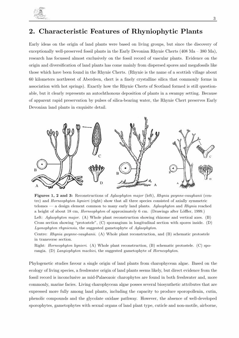
Figures 1, 2 and 3: Reconstructions of Aglaophyton major (left), Rhynia gwynne-vaughanii (cen-
tre) and Horneophyton lignieri (right) show that all three species consisted of axially symmetric
telomes — a design element common to many early land plants. Aglaophyton and Rhynia reached
a height of about 18 cm, Horneophyton of approximately 6 cm. (Drawings after Loffler, 1999.)
Left: Aglaophyton major. (A) Whole plant reconstruction showing rhizome and vertical axes. (B)
Cross section showing “protostele”, (C) sporangium in longitudinal section with spores inside. (D)
Lyonophyton rhyniensis, the suggested gametophyte of Aglaophyton.
Centre: Rhynia gwynne-vaughanii. (A) Whole plant reconstruction, and (B) schematic protostele
in transverse section.
Right: Horneophyton lignieri. (A) Whole plant reconstruction, (B) schematic protostele. (C) spo-
rangia. (D) Langiophyton mackiei, the suggested gametophyte of Horneophyton.
Phylogenetic studies favour a single origin of land plants from charophycean algae. Based on the
ecology of living species, a freshwater origin of land plants seems likely, but direct evidence from the
fossil record is inconclusive as mid-Palaeozoic charophytes are found in both freshwater and, more
commonly, marine facies. Living charophycean algae posses several biosynthetic attributes that are
expressed more fully among land plants, including the capacity to produce sporopollenin, cutin,
phenolic compounds and the glycolate oxidase pathway. However, the absence of well-developed
sporophytes, gametophytes with sexual organs of land plant type, cuticle and non-motile, airborne,

4
sporopollenin-walled spores suggests that these innovations evolved during the transition to the
land. In contrast to animal groups, the entire multicellular diploid phase of the plant life cycle
probably evolved in a terrestrial setting.
The transition from an aqueous to a gaseous medium exposed plants to new physical conditions that
resulted in key physiological and structural changes. Phylogenetic studies predict that early land
plants were small and morphologically simple, and this hypothesis is borne out by fossil evidence
(see Figures 1, 2 and 3). Early fossils bear a strong resemblance to the simple spore-producing
phase of living mosses and liverworts, and these similarities extend to the anatomical details of
the spore-bearing organs and the vascular system. The fossil record also documents significant
differences from living groups, particularly in life cycles and the early evolution of the sexual phase.
Figures 4, 5 and 6: Left: Several spore tetrades inside a sporangium of Aglaophyton major.
Centre: Germinating spore of Aglaophyton major with tongue-shaped young gametophytes.
Right: Lyonophyton rhyniensis, the suggested gametophyte of Aglaophyton. Section through the
longitudinal axes of two gametangiophores. (Photographies from Kerp & Hass, 1999.)
Land-plant life cycles are characterized by alternating multicellular sexual (haploid gametophyte, n)
and asexual phases (diploid sporophyte, 2n)(see Figures 4, 5 and 6). Phylogenetic studies indicate
that land plants inherited a multicellular gametophyte from their algal ancestors but that the
sporophyte evolved during the transition to the land. Most megafossils are sporophytes, and until
recently there was no direct early fossil evidence for the gametophyte phase. Recent discoveries of
gametophytes in the Rhynie Chert have shed new light on the evolution of land-plant life cycles.
Early gametophytes are more complex than in extant land plants and have branched stems bear-
ing sexual organs on terminal cup- or shield-like structures. Archegonia (female gametangia) are
flask-shaped with a neck canal and egg chamber, and are sunken as in hornworts and most vascular
plants. Antheridia (male gametangia) are roughly spherical, sessile or with a poorly-defined stalk,
and superficial. Gametophytes are very similar to associated sporophytes, and shared anatomi-
cal features (water-conducting tissues, epidermal patterns, and stomates) have been used to link
5
corresponding elements of the life cycle. Provisional reconstructions of the life cycle of an early
vascular plant are based on information from anatomically preserved plants and contemporaneous
compression fossils (see Kenrick & Crane, 1997).
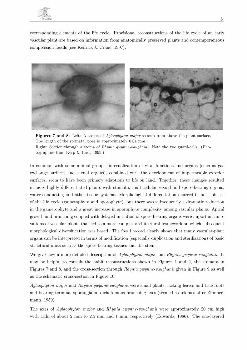
Figures 7 and 8: Left: A stoma of Aglaophyton major as seen from above the plant surface.
The length of the stomatal pore is approximately 0.04 mm.
Right: Section through a stoma of Rhynia gwynne-vaughanii. Note the two guard-cells. (Pho-
tographies from Kerp & Hass, 1999.)
In common with some animal groups, internalization of vital functions and organs (such as gas
exchange surfaces and sexual organs), combined with the development of impermeable exterior
surfaces, seem to have been primary adaptions to life on land. Together, these changes resulted
in more highly differentiated plants with stomata, multicellular sexual and spore-bearing organs,
water-conducting and other tissue systems. Morphological differentiation ocurred in both phases
of the life cycle (gametophyte and sporophyte), but there was subsequently a dramatic reduction
in the gametophyte and a great increase in sporophyte complexity among vascular plants. Apical
growth and branching coupled with delayed initiation of spore-bearing organs were important inno-
vations of vascular plants that led to a more complex architectural framework on which subsequent
morphological diversification was based. The fossil record clearly shows that many vascular-plant
organs can be interpreted in terms of modification (especially duplication and sterilization) of basic
structural units such as the spore-bearing tissues and the stem.
We give now a more detailed description of Aglaophyton major and Rhynia gwynne-vaughanii. It
may be helpful to consult the habit reconstructions shown in Figures 1 and 2, the stomata in
Figures 7 and 8, and the cross-section through Rhynia gwynne-vaughanii given in Figure 9 as well
as the schematic cross-section in Figure 10.
Aglaophyton major and Rhynia gwynne-vaughanii were small plants, lacking leaves and true roots
and bearing terminal sporangia on dichotomous branching axes (termed as telomes after Zimmer-
mann, 1959).
The axes of Aglaophyton major and Rhynia gwynne-vaughanii were approximately 20 cm high
with radii of about 2 mm to 2.5 mm and 1 mm, respectively (Edwards, 1986). The one-layered
6
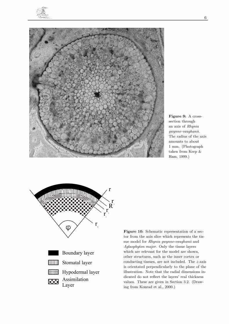
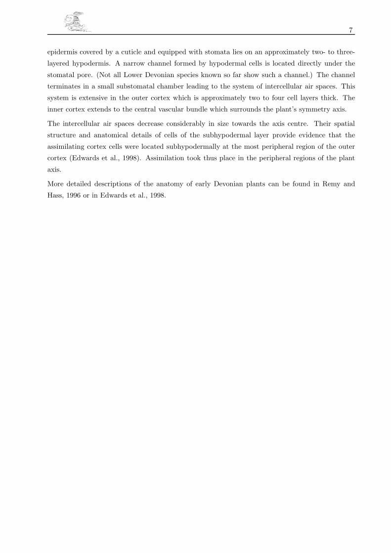
Figure 9: A cross-
section through
an axis of Rhynia
gwynne-vaughanii.
The radius of the axis
amounts to about
1 mm. (Photograph
taken from Kerp &
Hass, 1999.)
Figure 10: Schematic representation of a sec-
tor from the axis slice which represents the tis-
sue model for Rhynia gwynne-vaughanii and
Aglaophyton major. Only the tissue layers
which are relevant for the model are shown,
other structures, such as the inner cortex or
conducting tissues, are not included. The z-axis
is orientated perpendicularly to the plane of the
illustration. Note that the radial dimensions in-
dicated do not reflect the layers’ real thickness
values. These are given in Section 3.2. (Draw-
ing from Konrad et al., 2000.)
7
epidermis covered by a cuticle and equipped with stomata lies on an approximately two- to three-
layered hypodermis. A narrow channel formed by hypodermal cells is located directly under the
stomatal pore. (Not all Lower Devonian species known so far show such a channel.) The channel
terminates in a small substomatal chamber leading to the system of intercellular air spaces. This
system is extensive in the outer cortex which is approximately two to four cell layers thick. The
inner cortex extends to the central vascular bundle which surrounds the plant’s symmetry axis.
The intercellular air spaces decrease considerably in size towards the axis centre. Their spatial
structure and anatomical details of cells of the subhypodermal layer provide evidence that the
assimilating cortex cells were located subhypodermally at the most peripheral region of the outer
cortex (Edwards et al., 1998). Assimilation took thus place in the peripheral regions of the plant
axis.
More detailed descriptions of the anatomy of early Devonian plants can be found in Remy and
Hass, 1996 or in Edwards et al., 1998.

8
3. The Mathematical Model
3.1 The Process of Diffusion
The movement of water vapour and carbon dioxide in plants is governed by the process of dif-
fusion, i.e. the tendency of gases and fluids to equalize differences in molecular concentration by
establishing a molecular current from areas of high to areas of low concentration. Fick’s first law
�j = −S grad C (3.1)
([�j] = mol/m2/s, [S] = m2/s, [C] = mol/m3) states that the current density �j (number of molecules
diffusing in time through area normal to the direction of movement) should be proportional to (i)
the concentration gradient and (ii) an effective conductance S which depends on the properties of
the diffusing molecules and on the medium through which they propagate2.
The derivation of Fick’s first law uses the basic idea of kinetic theory: the molecules of a gas
(or a fluid) collide with one another and with the walls of their container. At room temperature
(T ≈ 300 ◦K) and atmospheric pressure (p = 1 atm) the collision frequency of a molecule is about
2× 10⁹ times per second. Energy and momentum among the molecules are hereby transferred and
the molecular current of (3.1) results. Detailed calculations (see, for instance, Reif, 1974) show
that the validity of equation (3.1) rests on two assumptions:
(i) not more than two molecules interact at the same time, which is equivalent to the statement
that the diameter d of a molecule is much smaller than its mean free path length lp (the mean
free path length is the average distance a molecule travels between two collisions),
d � lp (3.2)
(ii) the molecules collide predominantly with other molecules rather than with the walls of their
container, i.e. the mean free path length lp should be much smaller than a typical linear
dimension L of the container, that is
lp � L (3.3)
For “air molecules” moving at room temperature and atmospheric pressure through a stoma of
Aglaophyton major or Rhynia gwynne-vaughanii with a diameter L of the stomatal pore we have
d ≈ 2 × 10⁻¹⁰m, lp ≈ 3 × 10⁻⁷m and L ≈ 2 × 10⁻⁵m. (3.2) and (3.3) are thus fulfilled.
In order to derive the Diffusion Equation (also known as Fick’s second law) we need a second
component besides (3.1), the principle of mass conservation. It states the intuitively evident fact,
that a temporal change in the number of molecules within a given volume ∂C/∂t is due to (at most)
2 The gradient of a function is defined in the appendix.

9
two reasons: (i) molecules enter or leave the volume via the flux �j and/or (ii) molecules within the
volume disintegrate into or are built up from their constituents. These processes are summarized
in the source strength Q. In mathematical language, this reads
∂C
∂t= div�j + Q (3.4)
Insertion of (3.1) into (3.4) leads to3
∂C
∂t= Q − div (S grad C) = Q − S ∆C − grad S grad C (3.5)
In polar coordinates (r, ϕ, z), defined by
x = r cos ϕ
y = r sin ϕ (3.6)
z = z
and
0 ≤ r < ∞ 0 ≤ ϕ < 2π −∞ < z < ∞
equation (3.5) becomes
S1r
∂
∂r
(r∂C
∂r
)+
1r2
∂
∂ϕ
(S
∂C
∂ϕ
)+
∂
∂z
(S
∂C
∂z
)− ∂C
∂t+
∂S
∂r
∂C
∂r= −Q (3.7)
If the source (or sink) term Q = Q(r, ϕ, z, t, C) ([Q] = mol/m3/s) is a linear function of C and if
the effective conductance S = S(r, ϕ, z) ([S] =m2/s) and appropriate boundary conditions are pre-
scribed, the diffusion equation (3.7) has exactly one solution for the concentration C = C(r, ϕ, z, t)
of water vapour or carbon dioxide. C(r, ϕ, z, t) represents a function of space and time and it is
valid for the whole plant or plant parts4. Once C = C(r, ϕ, z, t) is calculated the current density�j(r, ϕ, z, t) follows from (3.1). This reads in polar coordinates
�j = −S(r, ϕ, z)(
∂C
∂r�er +
1r
∂C
∂ϕ�eϕ +
∂C
∂z�ez
)(3.8)
where �er, �eϕ and �ez are the system of orthonormal unit vectors in the directions r, ϕ and z,
respectively.
3 Definitions of the operators grad , div and ∆ can be found in the appendix.4 If Q(C) is a non-linear function, the boundary value problem may or may not have a well-defined
solution. This depends on the details of Q(C).
10
3.2 Diffusion in Rhyniophytic Plants — Problems and FurtherProceeding
It is impossible to solve (3.7) in all generality for realistic conditions, because the complex network
of voids and channels which form the intercellular air space (see Figure 9), the principal gateway for
carbon dioxide and water vapour, implies very complex boundary conditions for (3.7) (as long as we
insist on solutions that are valid down to the mean free path length lp of a molecule). If, however,
we claim that C and �j shall be correct only down to dimensions of a few diameters of a typical
cell, we can employ approximations which lead to symmetries that allow for drastic simplifications
in (3.7) and (3.8).
If we choose the second option, we can apply the porous medium approach, assume translatorial
symmetry along the plants symmetry axis and stationary conditions. Moreover, we can assume
that the effective conductance S remains constant within the functionally different tissue layers of
rhyniophytic plants. These approximations and some estimations of the possible errors caused by
their application will be discussed in the next section.
All terms with the exception of first on the left side of equation (3.7) disappear due to the afore-
mentioned assumptions and (3.7) transformes into the ordinary differential equation
1r
d
dr
(rdC
dr
)= −Q
SS = const. C = C(r) Q = Q(r,C(r)) (3.9)
which will be central to our approach. (3.8) reduces to
j(r) = −SdC(r)
dr(3.10)
where j is defined by �j = j �er.
The solution procedure will be as follows: After assigning appropriate values to S and specifying
Q(C) — after applying a quantitative model of photosynthesis — equation (3.9) must be solved
separately for each tissue layer. Because (3.9) is an ordinary differential equation of the second
order, each of the layer specific solutions contains two arbitrary constants. These constants will
be fixed in a second step by combining the layerspecific solutions in such a way that (i) C(r) and
j(r) become continuous functions of r, and, (ii) certain boundary conditions (which are explained
below) are satisfied.
3.3 Approximations
3.3.1 The porous medium approach
The overall structure of rhyniophytic plants with their concentric layers suggests axial symmetry.
If this would be true down to the dimensions of a cell, the orientation of the coordinate systems
z-axis along the plant’s symmetry axis would eliminate the ϕ-dependance of C and S (compare

11
Figure 11). As a consequence, the second term on the right hand side of (3.7) would disappear. A
closer look at Figure 9 reveals, however, that the internal structures of the concentric layers consist
of cells and voids which do not fit the mathematically favourable axial symmetry of the overall
structure.
r
z
Figure 11: The coordinate system is oriented in such a
way that its z-axis coincides with the plant’s symmetry axis.
The coordinate r measures the (orthogonal) distance from
the symmetry axis and ϕ revolves around the symmetry
axis in a plane z=const., attaining values between 0 and 2π.
In order to establish axial symmetry despite this difficulty, we apply the porous medium approxi-
mation.
The porous medium approach is widely used (but seldom stated explicitly) as a tool in Applied
Geology in order to describe the flow of water (via Darcy’s law) or the transport processes of
contaminants in soils and aquifers (via Fick’s laws) (see, for instance, Grathwohl, 1998). It was
developed by engineers who deal with industrial processes which take place in porous media (Aris,
1975). It was was applied to plant leaf tissue by Parkhurst & Mott (1990) in order to study the
gradients of intercellular carbon dioxide concentrations inside angiosperm leaves (see also the review
by Parkhurst, 1994 and literature cited therein).
The central idea of the porous medium approach is the replacement of the discontinuous arrange-
ment of cells and voids inside the real plant by a fictitious tissue whose continuous material proper-
ties are partly attributable to the cells and partly to the voids of the real plant. This is achieved by
an averaging process which reduces the complex geometrical details of the cell and void architecture
to just two quantities, the porosity n and the tortuosity τ , defined by
n :=Vp
V(3.11)
with Vp the pore volume and V the total volume of a volume element, and
τ :=lel
(3.12)
12
with le denoting the length of the actual path which a molecule has to follow in order to move from
one given point to another and l the (geometrically) shortest distance between these same points.
The effective conductance S is defined in terms of n, τ and the free air conductance D via
S := Dn
τ2(3.13)
The price of this simplification is obvious: Some information about the geometry of the cells and
voids of the plant tissue gets irrecoverably lost due to the averaging process. Other parts of the
knowledge on the plant geometry are condensed and shifted into the quantity S. S will turn
out later on to be a piecewise constant factor (and not even a non-trivial scalar function) in the
differential equation (3.7) itself. This simplifies the solution process considerably. Moreover, we
gain very simple boundary conditions for (3.7) in the geometrical shape of a circle, which are much
easier to handle than boundary conditions specified on the irregular boundaries between voids and
cells in Figure 9.
The porous medium approximation raises the lower limit of the validity of equation (3.7) and of its
solutions from the mean free path length lp of the carbon dioxide or water vapour molecules to a
few diameters of a typical plant cell.
The independence of C and S from the coordinate ϕ is now established: once the differences
between cells and voids have been eliminated by the averaging approach, the axial symmetry of the
“macroscopic” scale is no longer disturbed and the second term in equation (3.7) disappears.
C
C
A
A
x=l
x=le
le
lee
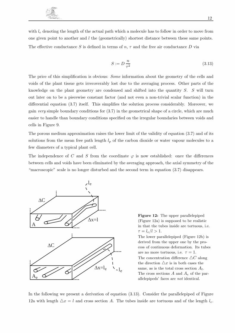
Figure 12: The upper parallelepiped
(Figure 12a) is supposed to be realistic
in that the tubes inside are tortuous, i.e.
τ = le/l > 1.
The lower parallelepiped (Figure 12b) is
derived from the upper one by the pro-
cess of continuous deformation. Its tubes
are no more tortuous, i.e. τ = 1.
The concentration difference �C along
the direction �x is in both cases the
same, as is the total cross section At.
The cross sections A and Ae of the par-
allelepipeds’ faces are not identical.
In the following we present a derivation of equation (3.13). Consider the parallelepiped of Figure
12a with length �x = l and cross section A. The tubes inside are tortuous and of the length le.
13
They point essentially into the x-direction. We denote the sum of the cross sections of all tubes by
At and the concentration difference along �x by �C.
The parallelepiped of Figure 12b has straight tubes, the length �x = le and the cross section
Ae. It is derived from the one in Figure 12a by continuous deformation, subject to the following
constraints:
(i) the deformation process affects neither the tube length �x = le nor the tubes’ total cross
section At ,
(ii) the volume V remains constant, i.e.
V = A l = Ae le (3.14)
(iii) the porosity n remains constant, i.e.
n =At leA l
=At leAe le
=At
Ae(3.15)
(iv) the concentration difference along �x varies in both cases by the amount �C,
(v) the deformation process does not affect the total current I, i.e.
I = −St At�C
l= −D At
�C
le(3.16)
Application of the “free air version” �j = −D grad C of equation (3.1) to the interior of the straight
tubes of Figure 12b and subsequent multiplication with At (under the assumption that the tubes
are much longer than their diameters) yields the last term of equation (3.16). Solving (3.16) for
the effective conductance St (which takes into account the tortuous nature of the tubes in Figure
12a) results in
St = Dl
le=
D
τ(3.17)
where (3.12) has been used.
In order to arrive at the version of Fick’s first law which is appropriate within the framework
of the porous medium approximation, we must “average out” the distinction between tubes and
impermeable parts of the parallelepiped. This is done by dividing the total current I by the cross
section A, thus giving rise to the (fictitious) current density
j =I
A(3.18)
Insertion of (3.16) into (3.18), (3.17), (3.15) and (3.12) leads to
j = −D
τ
At
A
�C
l= −D
n
τ2
�C
�x= −D
n
τ2grad C (3.19)
14
Comparison with (3.1) yields the desired result
S = Dn
τ2(3.20)
We emphasize that fluxes (i.e current densities in mol/m2/s) calculated by using the porous medium
approximation via (3.19) show other numerical values than real fluxes measured within the plant’s
voids (e.g. the intercellular airspace). Measured values of concentrations (in mol/m3), however,
should attain the same values as those calculated in the framework of the porous medium approx-
imation.
3.3.2 Translatorial symmetry
As the height of a rhyniophytic plant exceeds the plant radius considerably, we can assume that the
fluxes of carbon dioxide and water vapour are oriented mainly radially, i.e. perpendicular to the
plant’s symmetry axis. If we orientate the coordinate system in such a way that the z-axis coincides
with the plant’s symmetry axis, C and S do not depend on z and the third term in equation (3.7)
becomes zero.
This is not quite true near the top and the bottom of the plant. There the molecules do not move
strictly radially. To estimate the error caused by ignoring this fact we assume that the flux through
a given area of the plant’s surface is proportional to this area:
error ≈ flux through tipstotal flux
≈ area of tipstotal area
=2πR2
2πR2 + 2πRh=
RR + h
≈ Rh−(
Rh
)2
(3.21)
where we have used the assumption R � h. Typical values for Aglaophyton major (h ≈ 20
cm, R ≈ 2 mm) and Rhynia gwynne-vaughanii (h ≈ 20 cm, R ≈ 0.5 mm) result in errors of
approximately 1 % and 0.25 %, respectively. This appears to be in an acceptable range.
3.3.3 Stationarity
We focus on situations which do not change with time, i.e. C and S do not depend on t and the
term ∂C/∂t in (3.7) disappears.
This condition is not as restrictive as it appears at first sight: a concentration front of, for example,
water vapour needs a time t ≈ s2/4DairH2O
= 0.01 s to diffuse a distance s = 1mm through free air.
The information that a change of humidity outside a plant (as caused by a sudden shower) has
taken place needs roughly the same time to propagate to the plant’s center. Stationary conditions
— on a perhaps different level than before — should therefore reestablish very quickly.
Since carbon dioxide molecules are heavier than water molecules, they move slightly slower in air
than water vapour molecules, but at the same order of magnitude. For the distance s = 1mm they
would need a time t ≈ s2/4DairCO2
= 0.017 s. (The diffusion constant of carbon dioxide in air is
DairCO2
= 1.51 × 10⁻⁵m2/s, that of water vapour in air is DairH2O
= 2.42 × 10⁻⁵m2/s.)

15
As a rule of thumb, the diffusion constant for a substance diffusing through water is about 10−4
times its value in air. The carbon dioxide molecules travel the greater part of their journey from
the free atmosphere through the intercellular airspace to the chloroplasts in airfilled voids, but once
they have entered a cortex cell, they must diffuse for a distance of roughly s = 5× 10⁻⁶m through
an aqueous solution. With DwaterCO2
= 1.7 × 10⁻⁹m2/s this takes a time t ≈ 0.004 s. It is therefore
still justified, to assume stationary conditions.
It should be noted, that the “transport velocity”5 of diffusion decreases with increasing distance:
a water vapour front diffusing through air would require a time span t ≈ (100)2 × 0.01 s = 100 s in
order to cover a distance of s = 100mm. This result is contrary to our intuition which — according
to our experince with bicycles and cars — expects proportionality between time and distance.
In the case of diffusion, however, time is proportional to the square of distance and velocity is
proportional to the reciprocal of distance.
3.3.4 Constancy of effective conductance S
The axis of a rhyniophytic plant consists of various tissue layers (e.g. stomatal, hypodermal,
assimilation layers, see Section 2 and Figures 9 and 10). The geometric properties porosity n and
tortuosity τ which influence the effective conductance S = D n/τ2 change more or less abruptly
between adjacent layers, but vary only slightly within the individual layers. As we shall calculate
later on, the effective conductance S may increase abruptly between neighbouring layers by a factor
of 104. Small variations of S within the layers appear thus negligible and we can assume S = const.
within the layers. As a result, the last term on the left hand side of (3.7) becomes zero.
In order to refine this somewhat crude argument in a more quantitative way, we shall now solve
the differential equation (3.7) for C(r) on a layer bounded by r = ra and r = rb > ra outside the
assimilation region (i.e. Q = 0 is valid). Using the approximations introduced in Sections 3.3.1,
3.3.2 and 3.3.3 and Q = 0, we rewrite equation (3.7) in the form
S1r
∂
∂r
(r∂C
∂r
)+
∂S
∂r
∂C
∂r=
1r
∂
∂r
(S r
∂C
∂r
)(3.22)
Integration of (3.22) leads to
C(r) = A + B
∫dr
r S(r)(3.23)
where A and B are constants of integration. The integration in (3.23) cannot be performed unless
the r-dependance of S(r) is explicitly given, which is impossible, because we do not know it. A
way out of this dilemma consists in expanding S(r) into a Taylor series in r and to throw away all
terms of higher than linear order. This is certainly justified, since we assume from the outset, that
5 With diffusion the notion of transport velocity is not as clear-cut as for a point particle, because there
is no unequivocal way to define something tangible like a “diffusion front” for a cloud of statistically
independently moving molecules.

16
within the layer ra < r < rb the function S(r) varies only slowly (if at all). The ansatz for S(r) is
thus
S(r) = S0 + S1r − rs
�r(3.24)
with the proviso
S1
S0� 1 (3.25)
and the definitions
rs :=ra + rb
2and �r := rb − ra (3.26)
Insertion of (3.24) into (3.23), integration, application of the boundary conditions
C(ra) = Ca and C(rb) = Cb (3.27)
and expansion of the result according to (3.25) leads to
C(r) =Cb ln
r
ra− Ca ln
r
rb
lnrb
ra
+S1
S0
�C
�r
(ln
rb
ra
)2
(�r ln r − r ln
rb
ra+ ra ln rb − rb ln ra
)(3.28)
with �C := Cb − Ca
The first term in equation (3.28) stems from the constant term in equation (3.24), the second term
in (3.28) — we abbreviate it henceforth by δC —, is produced by the term proportional to S1 in
(3.24), which represents the slowly varying part in S(r) (that is, if there is any variation at all).
This can be seen by putting S1 = 0 in both equations.
Using ln r ≤ ln rb, −r ln (rb/ra) ≤ −ra ln (rb/ra) and ln (rb/ra) ≥ 1 (all of which follow from ra ≤ rb
and the isotony of the logarithm) we conclude the following chain of inequalities for the relative
error δC/�C
δC
�C=
S1
S0
(�r ln r − r ln
rb
ra+ ra ln rb − rb ln ra
)�r
(ln
rb
ra
)2 ≤ S1
S0
1
lnrb
ra
≤ S1
S0� 1 (3.29)
The result is an agreeable one: The relative error δC/�C caused in C(r) by neglecting a (possibly
existing) linear term S1 in S(r) is always smaller than the relative error S1/S0 in the function
S(r) = S0 + S1 (r − rs)/�r. In other words: small errors in S (as produced, for instance, whilst

17
measuring the porosity of a layer from thin sections like the one depicted in Figure 9) are not
“amplified” by the mathematics of our model, they rather tend to be averaged out in the result for
C(r).
In parentheses we remark, that S0 can be interpreted as the mean value S of the function S(r)
S :=
∫ rb
raS(r)dr∫ rb
radr
= S0 (3.30)
and S1 is proportional to the standard deviation ∆S of S(r)
∆S :=
√(S(r) − S
)2=
S1
2√
3(3.31)
Since mean value and standard deviation are the basic ingredients of linear regression analyses, it is
possible to analyze plots of the effective conductance S (or of the porosity n and/or the tortuosity
τ) against the variable r, in order to establish tight upper bounds on the relative error via (3.29)
δC
�C≤ S1
S0
1
lnrb
ra
≤ S1
S0(3.32)
The reduction of the equations (3.7) and (3.8) to equations (3.9) and (3.10), respectively, is thus
completed.
3.4 Photosynthesis
Before solving (3.9) for the assimilation layer we have to
— specify the model of photosynthesis which will be used to construct an explicit expression for
the carbon dioxide sink Q = Q(C) in equation (3.9), generated by assimilation and
— connect it to (3.9).
3.4.1 The Model of Photosynthesis — General Remarks
The mechanism of photosynthesis provides plants (and the animals feeding upon them) with struc-
tural materials and with the energy required for vital functions. Photosynthesis converts the
energy of electromagnetic radiation originating from the sun into chemical binding energy. First,
the radiation energy is absorbed and splits water into oxygen and hydrogen. Then, the hydrogen is
transferred along a long and complex chain of redox reactions to the carbon dioxide to form energy-
rich sugars that serve both as structural material and as energy store for metabolistic demands of
a plant6.
6 This is of course not the whole truth: The role of photosynthesis is also important for getting rid of the
entropy which is invariably produced when plants (and animals) build up and rebuild their structures
and when they transform chemical energy in order to sustain their life processes. If electromagnetic
radiation from the sun would not import negentropy into the food chains on earth (which means
exporting entropy), things would soon stand still.

18
As assimilation consumes (i) water, (ii) carbon dioxide and (iii) light, the assimilation rate (i.e
the release rate of assimilation products, like sugar or oxygen) should depend on the supply of
these three components. Plants, however, are able to close their stomata in order to minimize
water loss by transpiration. They also cut hereby their carbon dioxide supply which results in
— at least as far as C3-plants are concerned — more severe consequences for the assimilation
process than water shortage itself7. Therefore, with respect to photosynthesis, water shortage is
always “dominated” by carbon dioxide shortage and water supply as an independent variable can
be ignored in assimilation models.
Quantitative models of photosynthesis use the carbon dioxide consumption of chloroplasts per time
and chloroplast area Achl as a measure for the assimilation rate and describe it as a function of two
independent variables: (i) the carbon dioxide concentration (or, equivalently, the carbon dioxide
partial pressure q) and (ii) the irradiance I (i.e. the influx of photons per time and area of the
plant surface). Additional parameters describe either the physical environment of the chloroplasts
(e.g. temperature T , partial pressure of oxygen po), are derived from biochemistry (e.g. specificity
factor τ for Rubisco) or serve as fitting parameters (e.g. the Michaelis-Menten constants Kc and
Ko for carboxylation and oxygenation resp.). The parameters may vary from model to model.
We employ here the photosynthetic model of Harley & Sharkey, 1991 and Kirschbaum & Farquhar,
1984 (both based on an older model of Farquhar et al., 1980). The core of the model consists of
the equation
Achl(q, I) =(
1 − po
2τ q
)min{Wc(q),Wj(q, I)} (3.33)
with
Wc(q) : = Vmaxq
q + Kc
(1 +
po
Ko
) (3.34)
Wj(q, I) : = J(I) × q
4(q +
po
τ
) (3.35)
and
J(I) : =α I√
1 +(
α I
Jmax
)2(3.36)
The expression min{Wc(q),Wj(q, I)} denotes the smaller of Wc(q) and Wj(q, I) for given q and I.
The variables and parameters in (3.33) are defined as follows:
— Achl: carbon dioxide consumption per time and chloroplast area
— Wc(q): rate of carboxylation if limited by Rubisco activity
7 The amount of water consumed by photosynthesis is negligible compared with the water loss caused
by transpiration.

19
— Wj(q, I): rate of carboxylation if limited by electron transport
— po: partial pressure of oxygen in the chloroplasts
— τ := KoVc,max/(KcVo,max): specificity factor of Rubisco
— Ko: Michaelis-Menten constant of oxygenation
— Kc: Michaelis-Menten constant of carboxylation
— Vmax ≡ Vc,max: maximum rate of carboxylation
— Vo,max: maximum rate of oxygenation
— J : potential rate of electron transport
— I: irradiance
— Jmax: light-saturated rate of electron transport
— α: efficiency of light conversion
The functional form of Achl(q, I) does not represent the outcome of a conclusive biochemical theory
of photosynthesis that has been derived from first principles of biochemistry and reaction kinetics.
It is rather an attempt to describe certain qualitative aspects of C3-plant specific photosynthesis
in a heuristic way (Parkhurst, 1994).
We shall now discuss the structure of (3.33) in terms of its biochemical and kinetic background.
As stated above, the goal of photosynthesis is to produce energy-rich carbonhydrates which can be
used by the plant’s metabolism. An important intermediate step is the fixation of carbon dioxide
in the pentose (sugar) molecule ribulose-1,5-biphosphate (RuBP). This reaction is very sensitive
with respect to
(i) the supply with carbon dioxide, i.e. the carbon dioxide partial pressure q,
(ii) the supply with RuBP, whose regeneration within the Calvin cycle depends on a sufficient
number of electrons being transported along the redox chain from water to carbon dioxide,
a process which consumes necessarily radiation energy and thus depends ultimately on the
irradiance I, and
(iii) the supply with and the catalytic activity of the enzyme ribulose-1,5-biphosphate-carboxyl-
ase/oxygenase (Rubisco), which performs the actual binding between carbon dioxide and
RuBP.
The situation is considerably complicated by a feature of Rubisco: Rubisco is a bifunctional enzyme,
it catalyses not only the reaction of carbon dioxide with RuBP (“carboxylation”) but also the
reaction of molecular oxygen with RuBP (“oxygenation”) at the same catalytic site. Oxygen and
carbon dioxide are thus mutually competitive inhibitors with respect to the activity of Rubisco.
The assimilation model (3.33) incorporates the features (i), (ii) and (iii) in the following way.
(i) The min-operation in (3.33) reflects the fact that the assimilation rate is limited by either the
rate of the ribulose-1,5-biphosphate (RuBP) regeneration via electron transport, described by
Wj(q, I), equation (3.35), or the amount, activity and kinetic properties of the enzyme ribulose-
1,5-biphosphate-carboxylase/oxygenase (Rubisco), quantitatively described by the function
Wc(q), equation (3.34). For given values of q and I, only the smaller of Wc(q) and Wj(q, I) is

20
therefore to be used in (3.33).
(ii) The factor 1 − po/2τq in (3.33) becomes negative for q < po/2τ (because the parameters in
equations (3.33) to (3.36) can attain only positive values, the functions Wc(q) and Wj(q, I) are
always positive). This expresses the fact that the chloroplasts produce more carbon dioxide
by photorespiration than they consume by photosynthesis, whenever the partial pressure q
of carbon dioxide in the chloroplasts drops below the carbon dioxide compensation point
Γ∗ := po/2τ . The chloroplasts’ carbon dioxide net consumption per time and area Achl attains
accordingly negative values.
This behaviour is a direct consequence of Rubisco’s nature as a bifunctional enzyme. Whether
Rubisco processes carbon dioxide or rather oxygen depends on the quantity
ϕ :=po
q
Kc Vo,max
Ko Vc,max=
po
q
1τ
(3.37)
i.e. on the partial pressures q and po of both gases, on Rubisco’s maximum rates of carboxy-
lation Vc,max and oxygenation Vo,max, and on the Michaelis-Menten constants Kc and Ko for
both processes.
The specificity factor
τ :=Ko Vc,max
Kc Vo,max(3.38)
can be understood as follows: Imagine some volume which contains as many oxygen as carbon
dioxide molecules together with a large amount of Rubisco. If after some time Rubisco has
catalyzed the binding between N oxygen and RuBP molecules, the number of carbon dioxide
molecules appended to RuBP will be τ N . As τ attains (depending on temperature) some
value between τ = 6, 741 (for T = 0 ◦C) and τ = 1, 906 (for T = 30 ◦C), Rubisco’s oxygenation
function may appear to be negligible. However, as stated above in equation (3.37), the ratio
ϕ of oxygenation to carboxylation is not given by τ alone. It is weighted with the ratio of the
partial pressures of oxygen and carbon dioxide. Today’s atmosphere is composed of about 20.95
% (volume %) oxygen and 0.03 % carbon dioxide. With τ = 2, 822 at T = 20 ◦C this amounts
to a ϕ = 0.2474. That is, if the oxygen/carbon dioxide ratio at an assimilating site would be
the same as in the free atmosphere, while carboxylating 100 RuBP-molecules Rubisco would
also oxygenate about 25 RuBP-molecules. In other words, about 20 % of Rubisco’s catalyzing
power would be involved in oxygenation.
(iii) We will now discuss how the dualistic activity of Rubisco affects Wc(q) and Wj(q, I) (equations
(3.34) and (3.35)). We begin with Wc(q).
Whether Rubisco processes carbon dioxide or rather oxygen depends on the quantity ϕ =
po/qτ = poKcVo,max/qKoVc,max (i.e. on the partial pressures q and po of both gases), on Ru-
bisco’s maximum rates of carboxylation Vc,max and oxygenation Vo,max, and on the Michaelis-
Menten constants Kc and Ko for both processes.

21
The hyperbola
Wc(q) := Vmaxq
q + Kc(3.39)
would be a good choice for a function which shall describe carboxylation if Rubisco would not
process oxygen. For large q values it approaches Vmax asymptotically, i.e. it shows “saturation
behaviour” and, for a given q, smaller values of the Michaelis-Menten constant Kc imply steeper
gradients in Wc(q). By choosing appropriate values for Vmax and Kc, the function Wc(q) can
thus be adjusted to experimentally obtained data. The introduction of fitting parameters
like a Michaelis-Menten constant indicates the heuristic nature of a theory: the behaviour of
a quantity as a function of the parameters that define a system cannot (yet) be calculated
from first principles but is obtained by adjusting arbitrary parameters like Vmax and Kc in a
qualitatively plausible relation such as the hyperbola Wc(q) in such a way that measured data
are reproduced.
Considering competitive inhibition, the rate of the carboxylation of RuBP in the presence of
competitive inhibition by oxygen with saturating RuBP is modelled by
Wc(q) = Vmaxq
q + Kc
(1 +
po
Ko
) (3.40)
Equation (3.40) is also a hyperbola. It
(a) approaches zero for q → 0,
(b) approaches asymptotically the maximum carboxylation rate Vmax for q → ∞ (the Calvin
cycle shows saturation behaviour with respect to carbon dioxide also in the presence of
oxygen), and
(c) takes into account the competitive inhibition by oxygen via the term Kc (1 + po/Ko) in
the denominator, which can be considered as an effective Michaelis-Menten “constant” for
carbon dioxide. (Here, effective means that it is rather a function of the oxygen partial
pressure po than a true constant. As before, higher values for po result in smaller gradients
of the function Wc(q). For po → 0 the term reduces to the “pure” Michaelis-Menten
constant Kc and Wc(q) reduces to Wc(q) from equation (3.40).)
We note that the structure of Wc(q) is by no means fixed by the conditions (a) to (c). There
exists an infinite variety of functions which satisfy (a) to (c), for instance
Wc(q) := Vmax tanh(
q Ko
Kc (Ko + po)
)or ˜
Wc(q) :=q√
q2 +(
Ko Vmax
Kc (Ko + po)
)2(3.41)
would behave similarly as Wc(q)8.
8 Stated more explicitly, Wc(q), Wc(q) and˜Wc(q) behave for very large and for small values of q in

22
(iv) We will now reconsider Rubisco’s bifunctional nature. In order to describe the rate of oxy-
genation of RuBP in the presence of competitive inhibition by carbon dioxide we can use
the same mathematical structure as in the case of carboxylation. This is possible because in
the biochemical mechanism responsible for inhibition, the roles of carbon dioxide and oxygen
are equivalent — with the consequence that within the mathematical structure the respective
variables are interchangeable. In more mathematical terms, this means that we perform the
substitutions
q ↔ po Kc ↔ Ko Vmax ↔ Vo,max (3.42)
The application on the function Wc(q) (equation (3.40)) results in
q Vmax
q + Kc
(1 +
po
Ko
) ↔ po Vo,max
po + Ko
(1 +
q
Kc
) (3.43)
The term Ko (1 + q/Kc) in the denominator can again be viewed as an effective Michaelis-
Menten “constant”, but now for oxygen, taking into account the competitive inhibition by
carbon dioxide.
If we use the definition of τ (see (3.38)) in order to eliminate Vo,max in favour of Vmax from
(3.43), we obtain
po Vo,max
po + Ko
(1 +
q
Kc
) =po
τ q× q Vmax
q + Kc
(1 +
po
Ko
) =po
τ q× Wc(q) (3.44)
where the final step follows from the definition of Wc(q), equation (3.34).
The net effect of this twofold Rubisco activity is given by
Wc(q) −12
po
τ q× Wc(q) =
(1 − po
2τ q
)× Wc(q) = Achl(q, I) (3.45)
which describes the carboxylation rate (3.34) minus half of the oxygenation rate (3.44) of RuBP.
The factor 1/2 that is inserted before (3.44) reflects the fact that for each two oxygenations
performed by Rubisco one molecule of carbon dioxide is released in photorespiration. The result
the same way:
(a) limq→∞ Wc(q) = limq→∞ Wc(q) = limq→∞˜Wc(q) = Vmax
(b) Wc(0) = Wc(0) = ˜Wc(0) = 0
(c) dWc/dq(0) = dWc/dq(0) = d˜Wc/dq(0) = Vmax/Kc(1 + po/Ko)
(d) (b) and (c) imply for small values of q: Wc(q) = Wc(q) = ˜Wc(q) ≈ q Vmax/Kc(1 + po/Ko)
23
is the net carbon dioxide consumption (per time and area) Achl (3.33) of the assimilating plant
tissue in the case Wj(q, I) > Wc(q).
(v) We discuss now the function Wj(q, I), which dominates Achl(q, I) for Wj(q, I) < Wc(q). Again,
it will appear twice, first as representing carboxylation and then as a description of its com-
petitive process, oxygenation. As stated above, for Wj(q, I) < Wc(q), the carboxylation rate is
given by the rate of the ribulose-1,5-biphosphate (RuBP) regeneration via electron transport,
equation (3.35)
Wj(q, I) = J(I)q
4(q +
po
τ
) (3.46)
If we interpret Wj(q, I) merely as a function of the variable q (and treat I as a constant) it
behaves — similarly as Wc(q) — as a hyperbola which
(a) becomes zero for q → 0 and
(b) approaches for q → ∞ asymptotically J/4, which is one fourth of the potential rate of
electron transport. The factor 1/4 appears because the regeneration of one molecule RuBP
in the Calvin cycle requires four electrons.
(c) The second term in the denominator, po/τ , is also involved in competitive inhibition of
carboxylation by oxygen. Although the RuBP regeneration by electron transport is not
directly affected by Rubisco’s bifunctional behaviour, the RuBP molecules, which are
oxygenated by Rubisco instead of being carboxylated, are lost for assimilation. Therefore
the term po/τ is included in the denominator. Again, higher values for po/τ result in
smaller gradients of the function Wj(q, I). For po → 0, however, the function reduces to
Wj(q, I) = J/4.
(vi) In order to calculate the rate of oxygenation performed on RuBP molecules we follow the same
ideas as we did above for Wc(q): We retain the mathematical structure of Wj(q, I) and submit
it to the transformation (3.42). As the specificity factor τ is defined in terms of Ko, Vc,max,
Kc and Vo,max it transforms under (3.42) as
Ko Vc,max
Kc Vo,max= τ → 1
τ=
Kc Vo,max
Ko Vc,max(3.47)
and the oxygenation rate becomes
J(I)po
4 (po + qτ)= J(I)
po
τ
4(po
τ+ q) =
po
τq× J(I)
q
4(po
τ+ q) =
po
τq× Wj(q, I) (3.48)
The net effect is — as above — given by the carboxylation rate (3.35) minus half of the
oxygenation rate (3.48) of RuBP.

24
Wj(q, I) − 12
po
τ q× Wj(q, I) =
(1 − po
2τ q
)× Wj(q, I) = Achl(q, I) (3.49)
provided Wj(q, I) < Wc(q) is valid.
(vii) The rate of carboxylation, if limited by electron transport, Wj(q, I), has the asymptotic value
J/4 (for q → ∞), where J is the potential rate of electron transport. That is, the potential for
electron transport of Wj(q, I) is exhausted only if the supply with carbon dioxide is plentiful.
J is not a constant but depends via equation (3.36) on the irradiance I (the number of photons
arriving per time and surface(!) area of the plant), and on the efficiency of light conversion α.
As the source of energy gained by the process of photosynthesis is electromagnetic radiation
with a wavelength shorter than about 700 nm, it is of no surprise that the intensity I of this
radiation is of importance.
The majority of the photons — typically around 80 % — is absorbed by photosynthetically
inactive tissue (Wullschleger, 1993). They do thus not reach the acceptors of the photosystems,
because they are “lost” during their way through the plant tissue. The fraction of the remaining
photons is denoted by α. αI is thus the number of photosynthetically active photons reaching
the chloroplasts. Obviously, rising numbers of photons I will raise the potential rate of electron
transport J , but experimental evidence indicates a saturation relation for J(I) as given in
equation (3.36)
J(I) =α I√
1 +(
α I
Jmax
)2(3.36)
Jmax, the light-saturated rate of electron transport, denotes the asymptotic value.
In other words: If the supply with light and carbon dioxide is unrestricted, the function Wj(q, I)
is still bounded, attaining the value
limI→∞
limq→∞ Wj(q, I) = lim
I→∞lim
q→∞
α I√1 +
(α I
Jmax
)2× q
4(q +
po
τ
) =
Jmax
4(3.50)
(viii) The assimilation model (3.33) does not provide for a light compensation point. This follows
because (i) Wj(q, I) > 0 for I > 0, and (ii) the only factor in Achl(q, I) which can become
negative, 1 − po/2τ , does not depend on I.
In preparation of constructing a linearized version of (3.33) we get rid of the min{ . , . }-operation
in (3.33).
Wc(q) and Wj(q, I) are hyperbolas with asymptotes and poles Wc(∞) = Vmax, qpole = −Kc (1 + po/Ko)
and Wj(∞, I) = J(I)/4, qpole = po/τ respectively. Therefore Wc(q) and Wj(q, I) intersect at at

25
most two points. For positive values of Kc, po, τ and Ko — which is guaranteed in view of their
physical interpretation as pressures — the first intersection is invariably tied to the origin of the
coordinate system at q = 0. The q-value of the second intersection
qs :=τKcJ(Ko + po) − 4VmaxKopo
τKo(4Vmax − J)(3.51)
however depends on the specifics of photosynthesis and can attain positive or negative values.
The relation between Wc(q) and Wj(q, I) can be characterized as follows: If qs ≤ 0 is valid,
Wc(q) and Wj(q, I) intersect nowhere along the (strict) positive part of the q-axis. Consequently,
Wj(∞, I) > Wc(∞) implies Wj(q, I) > Wc(q) for all q > 0, and vice versa. If, on the other hand,
qs > 0 is true, Wj(∞, I) > Wc(∞) implies Wj(q, I) > Wc(q) only for q-values greater than qs.
Because Wc(q) and Wj(q, I) intersect at qs they exchange their roles of dominating one another
and for q-values between 0 and qs follows Wj(q, I) < Wc(q). We can therefore write (3.33) in the
form
Achl(q, I) :=
Vmax
q − po
2τ
q + Kc
(1 +
po
Ko
)
if qs ≤ 0 and J/4 > Vmax
if qs > 0 and J/4 > Vmax and qs < q
if qs > 0 and J/4 < Vmax and 0 < q < qs
J(I)4
×q − po
2τq +
po
τ
if qs ≤ 0 and J/4 < Vmax
if qs > 0 and J/4 < Vmax and qs < q
if qs > 0 and J/4 > Vmax and 0 < q < qs
(3.52)
with
J(I) =α I√
1 +(
α I
Jmax
)2(3.36)
It appears that (3.52) is more complex than (3.33). Its benefits, however, will become visible later
on.
3.4.2 Connection between Diffusion and Photosynthesis
The implementation of the photosynthesis model (3.33) into the diffusion equation (3.9) requires
the following tasks:
(i) Achl(q, I) is to be connected to Q by bookkeeping considerations which involve
— the porosity nas of the plant’s outer cortex,
— the surface aas of a typical cortex cell,
— the volume vas of a typical cortex cell and
— the sum of the surfaces of all chloroplasts within one cortex cell achl.

26
These parameters have to be considered, because photosynthesis takes place in the chloro-
plasts located at the peripherie of an assimilating cell and the carbon dioxide flux depends on
geometrical relations (see equation (3.54)).
Consider a volume V which encompasses several cortex cells and the intercellular air spaces
between them. The left hand side of the equation
−QV ={
V
vas(1 − nas)
} [achl Achl(q, I)
](3.53)
regardes the number of molecules which are extracted per time from the diffusion current
which flows through the volume V according to equation (3.10). It should be balanced by the
right hand side, which consists of two factors: The entity in brackets is the product of the
flux Achl(q, I) and the area achl. It describes therefore the number of molecules flowing per
time into one cortex cell. As nas stands for the porosity, V (1 − nas) is the volume within V
occupied by assimilating cells. vas denotes the volume of one cortex cell. The entity in braces
gives thus just the number of cortex cells within V . The product of bracket and brace indicates
the number of molecules disappearing per time from the volume V and being processed in the
biochemical assimilation machine represented by Achl(q, I).
Division by V and rearrangement of the factors lead to
−Q =(
achl
aas
) (aas
vas
)(1 − nas)Achl(q, I) (3.54)
The ratio (achl/aas) between the sum of the surfaces of all chloroplasts achl within one cortex
cell and the surface aas of this cell and the surface to volume ratio (aas/vas) of a typical cortex
cell have been introduced in the last step, because these ratios are easier to calculate than the
individual factors from which they are built up.
Insertion of (3.54) into equation (3.9) and the relation S = D n/τ2 lead to the following
(intermediate) form of the diffusion equation in the assimilation layer:
d2C
dr2+
1r
dC
dr=
1DCO2
× τas2
(achl
aas
)(aas
vas
)1 − nas
nas× Achl(q, I) (3.55)
(ii) There remain two problems — a minor one and a more serious one — in (3.55): the left hand
side is an expression in C(r), the carbon dioxide concentration in the intercellular airspaces
of the assimilation layer, whereas its right hand side depends on the carbon dioxide partial
pressure q inside the chloroplasts. That means comparing different quantities which are —
still more important — defined at different places.
The minor problem is solved with the help of the equation of state of an ideal gas (carbon
dioxide at atmospheric pressure and temperature is a quite ideal gas). It connects the (partial)
pressure p of ν moles of an ideal gas at temperature T inside a volume V via the well-known
27
relation p V = νRgasT . Using the definition C := ν/V of (molar) concentration, p = RgasT×C
follows immediately.
The more serious problem will now be considered. In order to turn (3.55) into a meaningful
equation, we have to quantify how the carbon dioxide pathway from the intercellular airspace
to the chloroplasts influences the diffusion rate. Cortex cells of rhyniophytic plants, like their
modern counterparts, consisted presumably of cell walls, plasmalemmata, cytosols, chloroplast
limiting membranes, and chloroplast stroma. As the anatomical knowledge of the assimilation
region of fossilized specimen is restricted due to taphonomic reasons and only size and number
density of cortex cells are known, it is impossible to calculate effective conductances for the
diffusional pathway of carbon dioxide molecules by using anatomical parameters.
Instead, we follow Parkhurst & Mott, 1990, Parkhurst, 1994 and Nobel, 1999, and use the
ansatz
Achl = gliq (RgasT C(r) − q) (3.56)
which is a spatially averaged analogue to Fick’s first law (3.1). The quantity RgasT C − q, the
difference between the carbon dioxide partial pressure in the intercellular airspace and in the
chloroplasts, plays the role of the “driving force” of diffusion (similar to grad C in equation
(3.1)). The quantity gliq ([gliq ] = mol/m2/s/Pa) is the analogue of the effective conductance
S = D n/τ2 in (3.1). It contains in compressed form all information on the interior structures
of the cortex cells which is relevant for the diffusion of the carbon dioxide molecules. Due to
taphonomic reasons the value of gliq must be estimated from extant plants (see Parkhurst &
Mott, 1990). Note that the diffusion inside the cortex cells — described by gliq — takes place
not in air but in an aqueous solution.
After connecnting C and q by (3.56) we equate (3.56) with (3.33) and solve for q as a function
of C, obtaining the result
q =
12
(RgasT C − J
4gliq− po
τ
+
√(RgasT C − J
4gliq+
po
4
)2
+32
po
τ
)if Wj(q, I) < Wc(q)
12
(RgasT C −
[Kc
(1 +
po
Ko
)+
Vmax
gliq
]
+
√(RgasT C +
[Kc
(1 +
po
Ko
)+
Vmax
gliq
])2
+ 4VmaxRgasT
(po
2τRgasT− C
) )
if Wj(q, I) > Wc(q)(3.57)
28
Insertion of this result back into (3.56) leads to an expression for Achl in terms of C, so that via
(3.55) the differential equation (3.9) for the carbon dioxide concentration in the assimilating
region attains the form
d2C
dr2+
1r
dC
dr= aC + b +
√αC2 + β C + γ (3.58)
which causes problems, because
— a, b, α, β and γ are involved combinations of the photosynthetic and morphological
parameters in equations (3.33) and (3.55), and
— (3.58) is a highly non-linear differential equation.
3.4.3 Linear Approximation of the Model of Photosynthesis
As equation (3.58) is a nonlinear differential equation in C(r), it cannot be solved in closed form9.
In order to circumvent this problem, we make use of the freedom granted by the fact that Achl(q, I)
is only of qualitative nature. That is, we shall replace Achl(q, I) as given by (3.33) by a linear
approximation Achllin(q, I), which retains the crucial features of (3.33) and casts (3.58) into a linear
differential equation in C. The features of (3.33) which we want the linear approximation to retain
are:
(i) Achllin(q, I) shall show saturation behaviour and approach the smaller of Wc(∞) = Vmax and
Wj(∞, I) = J(I)/4 for large values of q asymptotically.
(ii) If q, the partial pressure of carbon dioxide at the assimilating site, drops below the carbon
dioxide compensation point Γ∗ = po/2τ , photorespiration will outweigh photosynthesis and
the chloroplasts’ net consumption (per time and area) of carbon dioxide Achllin(q, I) becomes
negative.
In other words: we want Achllin(q, I) to behave like Achl(q, I) (i) for very large values of q, and, (ii) for
small values of q, i.e. in the neighbourhood of q = 0 and q = Γ∗. (Γ∗ was defined as Γ∗ := po/2τ .)
To this end we define the linear approximation Achllin(q, I) to (3.52) by
(i) the straight line through the points (q,Achl) = (0, Achl(0, I)) and (q,Achl) = (Γ∗, 0), and,
(ii) the straight line parallel to the q-axis with the asymptotic value Achl = min{Vmax, J/4}.
that is,
9 To be more precise: There do exist closed solutions for special numerical values of the parameters
a, b, α, β and γ or, if certain relations between them are valid (For a trivial example try β =2√
αγ.) Closed solutions may exist under even less restrictive conditions, but then they are beyond
our knowledge. The crucial point, however, is not the information as such. Due to the non-linearity
of (3.58), solutions cannot be calculated in a systematic, or semi-systematic fashion. This is quite
different with linear differential equations. As they obey the principle of linear superposition, it is
always possible to gain an at least qualitative understanding of the behaviour of their solutions.
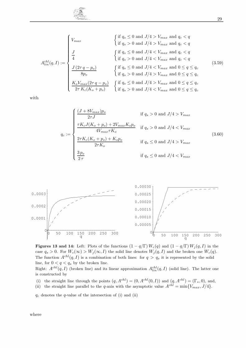
29
Achllin(q, I) :=
Vmax
{if qs ≤ 0 and J/4 > Vmax and qc < q
if qs > 0 and J/4 > Vmax and qc < q
J
4
{if qs ≤ 0 and J/4 < Vmax and qc < q
if qs > 0 and J/4 < Vmax and qc < q
J (2τ q − po)8po
{if qs ≤ 0 and J/4 < Vmax and 0 ≤ q ≤ qc
if qs > 0 and J/4 > Vmax and 0 ≤ q ≤ qc
KoVmax(2τ q − po)2τ Kc(Ko + po)
{if qs ≤ 0 and J/4 > Vmax and 0 ≤ q ≤ qc
if qs > 0 and J/4 < Vmax and 0 ≤ q ≤ qc
(3.59)
with
qc :=
(J + 8Vmax)po
2τJif qs > 0 and J/4 > Vmax
τKcJ(Ko + po) + 2VmaxKopo
4VmaxτKoif qs > 0 and J/4 < Vmax
2τKc(Ko + po) + Kopo
2τKoif qs ≤ 0 and J/4 > Vmax
3 po
2 τif qs ≤ 0 and J/4 < Vmax
(3.60)
0
0.0001
0.0002
0.0003
0 50 100 150 200 250 300q
0
0.00005
0.00010
0.00015
0.00020
0.00025
0.00030
0 50 100 150 200 250 300q
Figures 13 and 14: Left: Plots of the functions (1 − q/Γ)Wc(q) and (1 − q/Γ)Wj(q, I) in the
case qs > 0. For Wc(∞) > Wj(∞, I) the solid line denotes Wj(q, I) and the broken one Wc(q).The function Achl(q, I) is a combination of both lines: for q > qs it is represented by the solid
line, for 0 < q < qs by the broken line.
Right: Achl(q, I) (broken line) and its linear approximation Achllin(q, I) (solid line). The latter one
is constructed by
(i) the straight line through the points (q,Achl) = (0, Achl(0, I)) and (q,Achl) = (Γ∗, 0), and,
(ii) the straight line parallel to the q-axis with the asymptotic value Achl = min{Vmax, J/4}.
qc denotes the q-value of the intersection of (i) and (ii)
where

30
qs =τKcJ(Ko + po) − 4VmaxKopo
τKo(4Vmax − J)(3.51)
and
J(I) =α I√
1 +(
α I
Jmax
)2(3.36)
qc denotes the q-value of the intersection of (i) and (ii), qs was defined above as the q-value of the
second intersection point of Wc(q) and Wj(q, I) (the first one lies at q = 0). Figures 13 and 14
show plots of Achl(q, I) and Achllin(q, I) for the parameter values given in the appendix.
Next we repeat some steps from the non-linear case above, but now for Achllin(q, I) instead of
Achl(q, I): we equate (3.59) with
Achllin = gliq (RgasT C − q) (3.61)
and solve for q as a function of C. Instead of (3.57) we get
q =
RgasT C − Vmax
gliq
{if qs ≤ 0 and J/4 > Vmax and qc < q
if qs > 0 and J/4 > Vmax and qc ≤ q
RgasT C − J
4 gliq
{if qs ≤ 0 and J/4 < Vmax and qc < q
if qs > 0 and J/4 < Vmax and qc < q
8 gliqRgasTpo C + poJ
2 (4 gliqpo + τJ)
{if qs ≤ 0 and J/4 < Vmax and 0 ≤ q ≤ qc
if qs > 0 and J/4 > Vmax and 0 ≤ q ≤ qc
2τgliqRgasTKc(Ko + po)C + KoVmaxpo
2τ (gliqKc(Ko + po) + KoVmax)
{if qs ≤ 0 and J/4 > Vmax and 0 ≤ q ≤ qc
if qs > 0 and J/4 < Vmax and 0 ≤ q ≤ qc
(3.62)
We insert (3.62) back into (3.61) and obtain an expression for Achllin(C) which substitutes (3.52) (or
(3.33)):
Achllin(C) :=
Vmax
{if qs ≤ 0 and J/4 > Vmax and Cqc
≤ C
if qs > 0 and J/4 > Vmax and Cqc≤ C
J
4
{if qs ≤ 0 and J/4 < Vmax and Cqc
≤ C
if qs > 0 and J/4 < Vmax and Cqc< C
J gliq (2τ RgasT C − po)2(4gliqpo + τ J)
{if qs ≤ 0 and J/4 < Vmax and 0 ≤ C ≤ Cqc
if qs > 0 and J/4 > Vmax and 0 ≤ C ≤ Cqc
gliq KoVmax(2τ RgasT C − po)2τ [gliq Kc(Ko + po) + Ko Vmax]
{if qs ≤ 0 and J/4 > Vmax and 0 ≤ C ≤ Cqc
if qs > 0 and J/4 < Vmax and 0 ≤ C ≤ Cqc
(3.63)

31
The concentration Cqcin the intercellular airspace is the equivalent of the pressure qc in the
chloroplasts. It is obtained by setting q = qc and C = Cqcin (3.62) and solving for Cqc
. The
result is
Cqc:=
(J + 8Vmax)pogliq + 2VmaxτJ
2τJRgasTgliqif qs > 0 and J/4 > Vmax
gliqτKcJ(Ko + po) + VmaxKo(2gliqpo + τJ)4τVmaxKoRgasTgliq
if qs > 0 and J/4 < Vmax
2gliqτKc(Ko + po) + Ko(gliqpo + 2τVmax)2τKoRgasTgliq
if qs ≤ 0 and J/4 > Vmax
6gliqpo + τJ
4τRgasTgliqif qs ≤ 0 and J/4 < Vmax
(3.64)
By replacing Achl(q, I) in (3.55) by Achllin(C) (as given in (3.59)) we arrive at the linearized version
of the diffusion equation (3.9), valid for the assimilation layer:
d2C
dr2+
1r
dC
dr=
{χ if rc ≤ r ≤ r1
k2 C − κ if r0 ≤ r ≤ rc
(3.65)
χ, κ and k are defined by
χ :=1
DCO2
× τas2
(achl
aas
)(aas
vas
)1 − nas
nas×
Vmax if J/4 > Vmax
J
4if J/4 < Vmax
(3.66)
κ :=1
DCO2
× τas2
(achl
aas
)(aas
vas
)1 − nas
nas×
−Jgliqpo
(8 gliqpo + 2τJ)
{if qs ≤ 0 and J/4 < Vmax
if qs > 0 and J/4 > Vmax
−gliqVmaxKopo
2τ [gliqKc(Ko + po) + KoVmax]
{if qs ≤ 0 and J/4 > Vmax
if qs > 0 and J/4 < Vmax
(3.67)
k2 :=1
DCO2
× τas2
(achl
aas
)(aas
vas
)1 − nas
nas×
−Jτgliq RgasT
(4 gliqpo + τJ)
{if qs ≤ 0 and J/4 < Vmax
if qs > 0 and J/4 > Vmax
−gliqVmaxKo RgasT
gliqKc(Ko + po) + KoVmax
{if qs ≤ 0 and J/4 > Vmax
if qs > 0 and J/4 < Vmax
(3.68)
The parameter rc, which has been introduced into (3.65), is defined by

32
rc :=
r0 if C(r = r0, rc = r0) > Cqc
r1 if C(r = r1, rc = r1) < Cqc
r∗c if C(r = r0, rc = r0) < Cqcand C(r = r1, rc = r1) > Cqc
(3.69)
where r∗c is solution of the equation
C(r = r∗c , rc = r∗c ) = Cqc(3.70)
rc divides the assimilation area into two layers defined by r0 ≤ r ≤ rc and rc ≤ r ≤ r1, resp.. In the
outer part of the assimilation layer, photosynthesis then works in the “saturated mode” (i.e. the
case qc ≤ q in (3.59) or Cqc≤ C in (3.63)), and in the inner part of the layer in the “linear mode”
(i.e. 0 ≤ q ≤ qc in (3.59) or 0 ≤ C ≤ Cqcin (3.63)). Thus, the model allows the net production of
carbon dioxide only in the inner part of the assimilation layer. This is no real restriction, however,
because the extreme cases rc = r0 or rc = r1 — meaning that the complete layer assimilates either
in the saturated or in the linear mode, resp. — are covered by the mathematics of the model.
The splitting up of the assimilation layer into two sublayers deserves some justification. This will
be given in the next section, in which we will discuss details of the calculation of rc. Meanwhile,
we affirm sceptical readers, that (3.69) (with (3.70)) is not a definition in circles.
We note that the information contained in the right hand side of equation (3.65) divides into the
three categories of assumptions (and reliability) (according to (3.66), (3.67) and (3.68)) discussed
in Section 1: the first factor, 1/DCO2, is a time independent constant of nature, the second factor
contains — apart from (achl/aas) — measurable quantities obtained from the fossil record, and
the third factor reflects photosynthetic considerations for extant C3-plants. In contrast, the water
vapour flux depends only on the first two categories and is therefore not affected by evolutionary
changes of biochemical mechanisms which may have ocurred since the Lower Devonian.
3.5 The solution procedure
Before presenting explicit solutions of the Diffusion Equation we recapitulate in more mathematical
terms what alterations it experienced in the last few sections.
— We started with the most general form of the Diffusion Equation, (3.5). It was a second order
partial differential equation in the variable C, linear or non-linear, depending on the form
of the source strength Q(C). The introduction of polar coordinates transformed the outer
appearance of the equation into (3.7) but left its mathematical nature untouched.
— The symmetries and approximations of Section 3.3 turned (3.7) into an ordinary differential
equation of second order, given as equation (3.9). It is linear in the boundary, the stomatal
and the hypodermal layer, because these layers provide no sources for water vapour or carbon
dioxide, whereupon the term Q vanishes.
33
— In the assimilation area of the outer cortex equation (3.9) attains the nonlinear form (3.58),
because the mechanism of photosynthesis (see (3.33) or (3.52), Section 3.4.1) shows saturation
behaviour, which turns the source strength Q(C) into a non-linear function of the carbon
dioxide concentration C.
— In order to cope with the considerable mathematical difficulties caused by the non-linearities
in (3.58) we linearized the model of photosynthesis with the result represented by equation
(3.63) (Section 3.4.3), turning (3.58) into the linear ordinary second order differential equation
of (3.65).
Putting the layer specific versions together, we arrive at the following piecewise defined, linear
ordinary differential equation of second order:
d2Ci
dr2+
1r
dCi
dr=
0 if r1 ≤ r ≤ r3 (i.e. i = bl, st, hy)
χ if rc ≤ r ≤ r1 (i.e. i = as,“saturated mode” of photosynthesis)
k2 Ci − κ if r0 ≤ r ≤ rc (i.e. i = as,“linear mode” of photosynthesis)
(3.71)
with bl = boundary layer, st = stomata layer, hy = hypodermal layer, as = assimilation layer.
In the case of water vapour diffusion only the first line of (3.71) applies, because we assume that
the intercellular airspace of the outer cortex is constantly saturated with water vapour. The con-
centration of water vapour in this layer is therefore obtained from the Kelvin-Equation (see (3.76)
below).
In the case of carbon dioxide diffusion, the whole system of equations (3.71) is appropriate. χ, k,
and κ (equations (3.66) through (3.68)) are combinations of natural constants and of parameters
that characterize the model of photosynthesis and the plant’s morphology. rc (defined in equations
(3.69) and (3.70)) results from the application of the linear approximation to the photosynthesis
model. It divides the assimilation layer into two areas: an inner zone (r0 ≤ r ≤ rc), where
photosynthesis works in “linear mode” and carbon dioxide net production is allowed to take place,
and a peripheral zone (rc ≤ r ≤ r1), where photosynthesis is in “saturated mode” and carbon
dioxide is only consumed at a constant rate (constant in the sense of being independent from r).
In mathematical terms, (3.71) represents a boundary value problem for both gases. In order to
solve it, we have to match the layer specific solutions of (3.71) in such a way that the overall solution
C(r) becomes a continuously differentiable function of r such that C(r) (and — depending on the
circumstances — perhaps j(r)) assume arbitrarily prescribed values at the boundaries of the region
considered.
The standard procedure of solving second order differential equations which are piecewise defined,

34
such as (3.71) consists of the following steps:
(i) General solution of the diffusion equation.
General solutions of (3.71) can either be calculated or — more easily — found in text books
on Theoretical Physics (for example, Arfken, 1970 or Morse & Feshbach, 1953). For the case
of carbon dioxide diffusion, they are cited in (3.72) and for water vapour diffusion in (3.73).
In(x) and Kn(x) denote the modified Bessel functions of the first respective second kind of
order n according to the conventions of Abramowitz & Stegun, 1972.
The effective conductances are defined as Si := DairCO2
ni/τi2 and si := Dair
H2Oni/τi
2, resp..
Ai and Bi (resp. ai and bi) are arbitrary constants to which definite values will be assigned
during the course of the matching procedure.
r CCO2(r) jCO2(r)
r3
boundarylayer
Abl + Bbl ln( r
R
)−Sbl
Bbl
r
R
stomatallayer
Ast + Bst ln( r
R
)−Sst
Bst
r
r2
hypodermallayer
Ahy + Bhy ln( r
R
)−Shy
Bhy
r
r1
intracellularair space(outercortex)
A2 + B2 ln( r
R
)+
χ
4r2 −Sas
[B2
r+
χ
2r
]rc
A1 I0(kr) + B1 K0(kr) +κ
k2Sas k [−A1 I1(kr) + B1 K1(kr)]
r0
(3.72)
(ii) Conditions of continuity at inner boundaries. The solutions cited in (i) should be
matched at the (inner) boundaries between the plant’s layers such that C(r) and j(r) become
continuous functions of r.
The physical basis of the continuity requirement lies in the mobility of the molecules of a
gas (or a fluid), which prevents discontinuous concentrations and current densities. Within
the various layers, continuity is already guaranteed by the mathematical structure of (3.71).
Critical areas, for which continuity has to be explicitly ensured, are the boundaries which
separate the layers at r = R, r2, r1 and rc10. An analogous requirement for the fluxes stems
10 This can be traced to the fact that the differential equation (3.71) is piecewise — one layer, one piece
— defined. As pointed out in Section 3.3.4, the effective conductance S changes quite abruptly at
the layer boundaries at r = R, r2 and r1. Additionally, the right hand side of equation (3.71) is
discontinuous at r = r1 and r = rc.

35
r CH2O(r) jH2O(r)
r3
boundarylayer
abl + bbl ln( r
R
)−sbl
bbl
r
R
stomatallayer
ast + bst ln( r
R
)−sst
bst
r
r2
hypodermallayer
ahy + bhy ln( r
R
)−shy
bhy
r
r1
(3.73)
from the fact, that — with the sole exception of the assimilating outer cortex — molecules
should nowhere disappear or spontaneously appear. The boundaries between the radial layers
are again critical areas (compare Figure 10). The conditions of continuity are explicitly given
in equations (3.78) for the case of carbon dioxide and in equations (3.80) for water vapour.
(iii) Boundary conditions. The solutions given in (i) and processed in (ii) should be continuously
connected to prescribed boundary values for C(r) (and perhaps j(r)).
For carbon dioxide diffusion we make the following assumptions:
— The carbon dioxide current shall cease at the inner edge of the photosynthetic active
region, that is, jCO2(r) should fulfill
jCO2(r0) = 0 (3.74)
— We assign the value CCO2atm to the carbon dioxide concentration in the free atmosphere
outside the boundary layer . The boundary condition at r = r3 reads then
CCO2(r3) = CCO2atm (3.75)
In the case of water vapour diffusion we assume:
— The inner cortex of rhyniophytic plants is saturated with liquid water, that is supplied by
the central vascular bundle and evaporates in the intercellular voids of the outer cortex.
The water vapour concentration in the intercellular air space is therefore in equilibrium
with the liquid water in the cortex cells. If temperature T and pressure p are given, the
water vapour concentration can be calculated from tabulated saturation values CH2Osat of
water vapour in air above a plane water surface via the Kelvin equation (sometimes called
Thomson equation after Lord Kelvins civic name), which considers the pressure drop of
water vapour due to capillary effects in the cortex cells (for details see Nobel, 1999, p.
36
312). With σ denoting the radius of a typical cortex cell, V ml the molar volume of water
and γ the surface tension in a boundary surface which separates air and liquid water, the
boundary condition at r = r1 reads
CH2O(r1) = CH2Osat exp
(2V m
l γ
RgasT σ
)(3.76)
— The water vapour concentration CH2Oatm in the free atmosphere outside the boundary layer
may be arbitrarily chosen, according to our assumptions on the prevailing climate, i.e. the
boundary condition at r = r3 is
CH2O(r3) = CH2Oatm (3.77)
More explicit statements of the boundary conditions can be found in equations (3.79) for
the case of carbon dioxide and in equations (3.81) for water vapour.
As part of the matching procedure the hitherto unspecified arbitrary constants Ai, Bi, ai and bi
are given definite values, because otherwise continuity of CCO2(r), jCO2(r), CH2O(r) and jH2O(r)
cannot be achieved. In other words, the (total) number of arbitrary constants which are present in
the general solutions (3.72) and (3.73) have to be equal to the number of conditions of continuity at
r = R, r2, r1 and rc, plus the number of boundary conditions given by equations (3.74) to (3.77).
Insertion of the general solutions (3.72) into the continuity and boundary conditions results
in the case of carbon dioxide in the following system of ten linear equations for the ten un-
knowns Ai and Bi:
Abl = Ast
Ast + Bst ln(r2
R
)= Ahy + Bhy ln
(r2
R
)Ahy + Bhy ln
(r1
R
)= A2 + B2 ln
(r1
R
)+
χ
4r1
2
A2 + B2 ln(rc
R
)+
χ
4rc
2 = A1I0(krc) + B1K0(krc) +κ
k2
SblBbl = SstBst
SstBst = ShyBhy
ShyBhy
r1= Sas
[B2
r1+
χ
2r1
]B2
rc+
χ
2rc = k [A1I1(krc) − B1K1(krc)] (3.78)
0 = k [A1I1(kr0) − B1K1(kr0)]
CCO2atm = Abl + Bbl ln
(r3
R
)(3.79)

37
Equations (3.78) represent the eight conditions of continuity. The two equations (3.79) represent
the two boundary conditions.
The system of equations (3.78) and (3.79) can be solved for the Ai and Bi by mathematical standard
procedures like matrix inversion. By this step, Ai and Bi become functions of the parameters which
describe the anatomy and the photosynthesis apparatus of the plant, and the particulars of the
boundary conditions. Note, that quantities like χ, k, and κ or the Si are just shorthand expressions
for complex combinations concerning parameters of anatomy and photosynthesis. Reinsertion of
the Ai and Bi back into the solutions (3.72) will almost complete the solution process: CCO2 and
jCO2 depend afterwards on anatomical and photosynthetical parameters, the variable r and the
parameter rc which has been defined in (3.69) and (3.70).
What remains to be done (in the case of carbon dioxide diffusion) is to calculate rc and to explain
its significance. Figures 15, 16 and 17 depict typical shapes of the concentration CCO2 in the
assimilation layer and a part of the hypodermal layer under qualitatively different conditions.
Cqc
C
C(r)
rr0 1rrc
1
4
2
3
5
Figure 15: The “standard situations” of
assimilation:
— Curve 1: CCO2 > Cqcin the whole
assimilation layer, photosynthesis is
running everywhere in the saturated
mode.
— Curve 2: CCO2 < Cqcin the whole
assimilation layer, photosynthesis is
running in the linear mode in the
whole layer.
— Curve 3: CCO2 < Cqcand CCO2 <
CΓ∗ , photosynthesis is running in
the linear mode in the whole layer,
net production of carbon dioxide in
the area with CCO2 < CΓ∗ .
— Curve 4: CCO2 > Cqcfor rc ≤
r ≤ r1, CCO2 < Cqcfor r0 ≤
r ≤ rc. Photosynthesis is running in
saturated mode in the outer zone of
the assimilation layer, in the linear
mode in the inner sublayer.
— Curve 5: Modification of Curve 4
with net production of carbon diox-
ide in the area with CCO2 < CΓ∗ .
Figure 15 illustrates several “standard situations” when assimilation runs and the carbon dioxide
concentration decreases steadily from its highest value in the atmosphere to the inner border of the
assimilation layer at r = r0. Three typical situations (plus two “subsituations”) can develop:
— The carbon dioxide concentration is higher than its “threshold-value” Cqcin the whole assim-
ilation layer, i.e. plenty of carbon dioxide is available, photosynthesis runs everywhere in the

38
saturated mode (Curve 1, Figure 15).
— The carbon dioxide concentration is lower than its “threshold-value” Cqcin the entire assimi-
lation layer, i.e. carbon dioxide is scarce, photosynthesis runs in the linear mode in the whole
layer. The less carbon dioxide is available, the less is consumed (Curve 2, Figure 15).
Wherever in the assimilation layer the carbon dioxide concentration drops below the carbon
dioxide compensation point CΓ∗ net production of carbon dioxide takes place (Curve 3, Figure
15).
— The carbon dioxide concentration in the outer zone of the assimilation layer is higher than
Cqc, but lower in its inner zone. In this case, net production of carbon dioxide is allowed to
take place only in the inner sublayer with r0 ≤ r ≤ rc (rc denotes the border surface between
both sublayers.) (Curve 4, Figure 15).
Similarly as above, the carbon dioxide concentration can drop beyond CΓ∗ (Curve 5, Figure 15).
Cqc
C
C(r)
rr0 1r
6
7
Figure 16: “Non-standard situations” of
assimilation:
— Curve 6: CCO2 = CΓ∗ in the whole
plant, carboxylation and oxygena-
tion are performed at identical rates.
This situation may develop when the
stomata are fully closed.
— Curve 7: CCO2 < CΓ∗ in the whole
plant, CCO2 is produced by photo-
synthesis (and transported away).
Figure 16 illustrates two “non-standard situations”.
— If there is no connection between the free atmosphere and the plant’s interior (e.g. when the
stomata are fully closed) a situation like the one depicted in Curve 6 of Figure 16 should
develop: carboxylation and oxygenation are performed at identical rates, the carbon dioxide
concentration attains the constant value CΓ after some time.
— If the carbon dioxide content of the atmosphere is smaller than CΓ, we may expect Curve 7 of
Figure 16: a continously growing carbon dioxide concentration for decreasing r.

39
Cqc
C
C(r)
rr0 1r
9
8
10
11
Figure 17: “Hypothetical situations” of
assimilation:
— Curve 8: Carbon dioxide is con-
sumed in the interior part of the
assimilation layer but produced in
the exterior part. This is unrealistic
under stationary conditions.
— Curve 9: Carbon dioxide is con-
sumed in the whole assimilation
layer, CCO2 increases for decreasing
r. This is unrealistic under station-
ary conditions.
— Curve 10: CCO2 increases for de-
creasing r. This is unrealistic under
stationary conditions.
— Curve 11: Photosynthesis works al-
ternately in saturated and linear
modes. This is unrealistic under sta-
tionary conditions.
Figure 17, after all, illustrates “hypothetical situations”, that should never develop due to physio-
logical reasons — at least not under stationary circumstances.
— Two of them (Curves 8 and 9) are covered by our mathematical model (with rc = r1).
— However, the situations depicted in Curves 10 and 11 cannot be described within the framework
of the model. Curve 10 cannot develop, because the inner zone would work in saturated
photosynthesis mode and the outer one in linear mode, whereas the assumption underlying
our model is just to the contrary. The situation of Curve 11 would require that the assimilation
layer has to split up not only into two — as is assumed in our model — but into six layers,
that work alternately in saturated and linear modes11.
We were forced to postpone the calculation of rc until now, because the “constants” Ai and Bi
became functions of rc only after the application of the conditions of continuity (3.78). Before this
step, it makes no sense to apply and solve the equations
rc :=
r0 if CCO2(r = r0, rc = r0) > Cqc
r1 if CCO2(r = r1, rc = r1) < Cqc
r∗c if CCO2(r = r0, rc = r0) < Cqcand CCO2(r = r1, rc = r1) > Cqc
(3.69)
and
CCO2(r = r∗c , rc = r∗c ) = Cqc(3.70)
11 If desired, our model can be extended to encompass the situations of Curves 10 and 11.

40
But meanwhile the functional dependance of Ai and Bi from rc is known and the calculation of the
parameter rc from (3.69) and (3.70) is possible. Insertion of rc into CCO2(r) and jCO2(r) obtained
from (3.72) completes the solution process.
The mathematics of the process of water vapour diffusion is less complex: The six constants ai and
bi and the expressions for CH2O(r) and jH2O(r) are calculated by insertion of the general solutions
(3.73) into the continuity and boundary conditions. This leads to a system of six linear equations
for the six unknowns ai and bi:
abl = ast
ast + bst ln(r2
R
)= ahy + bhy ln
(r2
R
)sblbbl = sstbst
sstbst = shybhy (3.80)
CH2Oatm = abl + bbl ln
(r3
R
)ahy + bhy ln
(r1
R
)= CH2O
sat exp(
2V ml γ
RgasT σ
)(3.81)
The first and the fourth equation represent the two boundary conditions, the other equations the
four conditions of continuity.
The system (3.80) has to be solved for the ai and bi which become hereby functions of anatomical
parameters of the stomatal and hypodermal layers and of the appropriate boundary conditions.
Reinsertion of the ai and bi back into the solutions (3.73) will result in the final form of the
solutions CH2O(r) and jH2O(r).
It should be noted at this point that the use of a computer code, such as MAPLE, is strongly advised
for all calculations. Faced with the task of inverting a 10× 10-matrix — as presented by equations
(3.78) and (3.79) — by traditional pencil-and-paper methods even mathematical hardcore purists
resort gratefully to computer codes, which are capable of doing symbolic algebraic manipulations.
Even then, the expressions for C(r) and j(r) look frightful and have therefore been shifted to the
appendix. It has proven to be economical to transform — whenever possible — arithmetic results
obtained with the aid of the computer already in statu nascendi into the easier digestable form of
a plot.
41
4. Application of the Model to Aglaophyton major andRhynia gwynne-vaughanii
The model as outlined above applies to every axially symmetric plant which qualifies for the ap-
proximations stated in Section 3.3. We have to show yet, how the model and data which were
obtained from fossilized specimen are connected. The quantities which relate data and model to
each other are mainly the effective conductivities for carbon dioxide and water vapour and the
radii of the various layers. As the effective conductivities are essentially composed of porosity n
and tortuosity τ ,
Si
DCO2
=si
DH2O=
ni
τi2
(4.1)
We explain now, how the ni and the τi can be calculated in a general way from measurements
carried out with thin sections of fossilized plants. The data are obtained from material which was
prepared at the Institute of Geology and Palaeontology of the University of Munster. The methods
of preparation will be presented in Section 5. After insertion of data from specimen of Aglaophyton
major and Rhynia gwynne-vaughanii we shall be able to derive actual results.
4.1 Boundary layer
The first barrier encountered by a diffusing molecule is the boundary layer of air which envelopes
the plant. If air (or, in general, a fluid) flows around an object, a velocity gradient develops due
to the adhesion of the innermost air layer to the object (see, for example, Vogel, 1994). Thickness
dbl and kind of the boundary layer (laminar or turbulent) influence its conductance with respect
to diffusion. For the present case, we choose the approximation given in Nobel (1999, p. 274) for
a cylindrical body of radius R immersed in air with a (free air) wind velocity v:
dbl = 5.8 × 10⁻³m
√2Rv
1s
(4.2)
With R as the plants radius we define the outer edge of the boundary layer as
r3 := R + dbl (4.3)
As molecules move in air unhindered by any obstacles, porosity and tortuosity take the values
nbl = 1 and τbl = 1 (4.4) (4.5)
leading to
Sbl
DCO2
=sbl
DH2O=
nbl
τbl2
= 1 (4.6)

42
4.2 Stomatal layer
The effective conductance of the stomatal layer depends on the density of the stomata, their pore
size and the diffusivity of the gas. We consider only the case of fully opened stomata, due to two
reasons:
(i) stomatal closure requires a corresponding regulation function which is not readily available for
Devonian plants, and,
(ii) during the closing process the size of the stomatal pore may drop below a threshold value
below which interactions between the diffusing molecules and the cell walls become important.
Condition (3.3) is no longer fulfilled and Fick’s first law ought to be modified (Jarman, 1974,
Leuning, 1983, Reif, 1974).
r2 denotes the inner edge of the stomatal layer, dst the depth of stomatal pores and thus
r2 := R − dst (4.7)
Fossilized specimen will provide values for the number of stomata per unit surface area, νst, and
for the average area of stomatal pores, ast, of Aglaophyton major and Rhynia gwynne-vaughanii
(see Section 5).
As the pores are shaped like ellipses, numerical values of ast are obtained by measuring the shortest
diameter wst and the longest diameter hst of a pore. The pore area is calculated via the equation
for the area of an ellipse
ast =π
4wsthst (4.8)
In order to calculate the porosity we concentrate on a “slice” of length L along the symmetry axis
(see Figure ). We approximate the stomatal layer between R and r2 by a thin rectangular plate of
thickness dst and side lenghts L and π(R + r2), where the latter is the arithmetic mean between
the circumferences of the outer surface (at r = R) and the inner surface (at r = r2) of the stomatal
layer.
The volume of one stoma is approximately astdst = π4 wsthstdst, the number of stomata on
the slice of length L is νstLπ(R + r2), and therefore the pore volume Vp is given by Vp =π2
4 wsthstdst νstLπ(R + r2). Because the total volume of the slice is V = dstLπ(R + r2) and
nst = Vp/V we obtain
nst = ast νst =π
4wsthstνst (4.9)
In the case of the stomatal layer, tortuosity results not from obstacles inside the stomata, but from
the following effect (see Figure ): within the boundary layer, the surfaces of equal concentration of
water vapour (or carbon dioxide) are not exactly concentric cylinders (whose centres coincide with
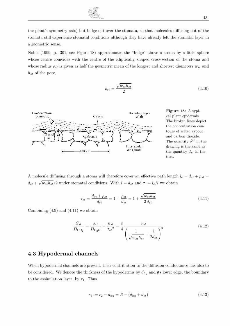
43
the plant’s symmetry axis) but bulge out over the stomata, so that molecules diffusing out of the
stomata still experience stomatal conditions although they have already left the stomatal layer in
a geometric sense.
Nobel (1999, p. 301, see Figure 18) approximates the “bulge” above a stoma by a little sphere
whose centre coincides with the centre of the elliptically shaped cross-section of the stoma and
whose radius ρst is given as half the geometric mean of the longest and shortest diameters wst and
hst of the pore,
ρst =√
wsthst
2(4.10)
Figure 18: A typi-
cal plant epidermis.
The broken lines depict
the concentration con-
tours of water vapour
and carbon dioxide.
The quantity δst in the
drawing is the same as
the quantity dst in the
text.
A molecule diffusing through a stoma will therefore cover an effective path length le = dst + ρst =
dst +√
wsthst/2 under stomatal conditions. With l = dst and τ := le/l we obtain
τst =dst + ρst
dst= 1 +
ρst
dst= 1 +
√wsthst
2 dst(4.11)
Combining (4.9) and (4.11) we obtain
Sst
DCO2
=sst
DH2O=
nst
τst2
=π
4νst(
1√wsthst
+1
2dst
)2 (4.12)
4.3 Hypodermal channels
When hypodermal channels are present, their contribution to the diffusion conductance has also to
be considered. We denote the thickness of the hypodermis by dhy and its lower edge, the boundary
to the assimilation layer, by r1. Thus
r1 := r2 − dhy = R − (dhy + dst) (4.13)
44
The same ideas as above are used in the derivation of porosity. Hypodermal channels, like stomata,
usually show an elliptic cross-sectional shape with a longer axis, hhy, and a shorter axis, why. Thus
their area is ahy = (π/4)hhywhy. Because every hypodermal channel is attached to exactly one
stoma, the number of hypodermal channels on a slice of length L equals the number of stomata,
νstLπ(R + r2). As the volume of one hypodermal channel is ahydhy = π4 whyhhydhy the total pore
volume of all channels reads Vp = π2
4whyhhydhy νstLπ(R+r2). The total volume of the hypodermal
“slice” is V = dhyLπ(r1 + r2), thus
nhy =Vp
V=
π
4hhywhy νst
2R − dst
2R − (2dst + dhy)(4.14)
where we have used (4.7) and (4.13).
Hypodermal channels contain no obstacles for diffusing molecules. Their tortuosity is therefore
τhy = 1 (4.15)
and the effective conductances become
Shy
DCO2
=shy
DH2O=
nhy
τhy2
=π
4hhywhy νst
2R − dst
2R − (2dst + dhy)(4.16)
4.4 Assimilation layer
The thickness of the assimilation layer is denoted as das and
r0 := r1 − das = R − (das + dhy + dst) (4.17)
represents its inner edge.
The outer cortex consists of cells whose shape is approximately cylindric. As the longitudinal axis
of these cells is parallel to the longitudinal axis of the plant, in cross-sectional view, the shape of
these cells is similar to circular disks. If we assume, that the cortex cells are either infintely long or
that their “end disks” are randomly distributed along the plant axis, rather than lying on common
cross-sections, the measurement of the (three-dimensional) porosity reduces two the evaluation of
(two-dimensional) cross-sections.
In Section 3.4.2 the specific surface (aas/vas) of a cortex cell was introduced. We denote the length
of a cell by L and its radius by σ. The disclike ends are cupped by half spheres with radius σ. The
expressions aas = 2πσL + 4πσ2 and vas = πσ2L + (4/3)πσ3 for the total surface and the volume
of the cylinder imply
(aas
vas
)=
2πσL + 4πσ2
πσ2L + (4/3)πσ3=
2σ×
1 + 2σ
L
1 +43
σ
L
(4.18)
45
For the limit of an infinite long cylindrical cell (L → ∞) this reduces to
(aas
vas
)=
2σ
(4.19)
For the sake of simplicity we will assume further on that this expression is valid.
In order to calculate the tortuosity of the outer cortex, we use a rough approximation: a molecule
which diffuses around such a cell has to move along a half circular path with a distance r from the
cell centre. The pathlength le amounts to le = πr, the direct distance is l = 2r, and the following
average value results:
τas =lel
=πr
2r=
π
2≈ 1.57 (4.20)
Once nas is explicitly known, the effective conductances can be calculated via
Sas
DCO2
=sas
DH2O=
nas
τas2
(4.21)
Another quantity of interest is the ratio (achl/aas) of the sum of the surfaces of all chloroplasts achl
within one cortex cell to the surface aas of this cell. It was introduced in (3.54) (Section 3.4.2) in
the light of the fact that this ratio can easier be calculated than the individual values achl and aas.
(achl/aas) is determined by two factors:
(i) Typical chloroplasts tend to look like oblate spheroids, whose shorter axes are about half as
long as their two (equally long) longer axes. Inside the cortex cells the chloroplasts seem to be
oriented in such a way, that their “equatorial planes” (defined by their longer axes) lie parallel
to the surfaces of the cortex cells. Therefore, if we denote the half-length of the longer axes
of a cortex cell by Rc, one chloroplast “covers” an area π Rc2 of the cortex cell’s surface area
aas. In other words, if the surface of a cortex cell would be entirely packed with chloroplasts,
each chloroplast’s supply of carbon dioxide would have to diffuse through an area π Rc2 of the
cortex cell’s surface, quite irrespective of the chloroplast’s surface.
The surface of a chloroplast showing the shape of an oblate spheroid is given by
Aη = 2πRc2 + πRc
2 η2√1 − η2
ln
(1 +
√1 − η2
1 −√
1 − η2
)(0 ≤ η ≤ 1) (4.22)
where Rc is the length of the spheroid’s longer and ηRc the length of its shorter half axis.
Therefore the ratio
Aη
πRc2 = 2 +
η2√1 − η2
ln
(1 +
√1 − η2
1 −√
1 − η2
)(4.23)
46
is one of the two factors, that cause the “area increase” (achl/aas) experienced by the carbon
dioxide diffusion current.
In the degenerate case η = 0 (the spheroid shrinks to a flat disk of radius Rc) we get A0/π Rc2 =
2 (the factor 2 stems from the fact, that even a degenerate, flat spheroid has two sides). η = 1
(the spheroid becomes a sphere of radius Rc) implies A1/πRc2 = 4 (as was to be expected).
For η = 1/2 (the spheroid’s shorter axis length is Rc/2) we arrive at A0.5/πRc2 = 2.760.
Values from the literature for the sizes of chloroplasts differ somewhat: Nultsch, 1996, gives as
chloroplast diameter the range 4 µm – 8 µm and as chloroplast depth 2 µm – 3 µm. Moore et.
al., 1998, give 5 µm – 10 µm and 3 µm – 4 µm, respectively. Calculating η from the averages
over the minima and maxima of these intervals we arrive at η = 3/7 = 0.429, which implies
A0.429/πRc2 = 2.606.
(ii) The second factor contributing to (achl/aas) is due to the fact that the (inner) surface of a
cortex cell is only partially lined with chloroplasts. Following Parkhurst & Mott, 1990, we
assume a value of 90 %.
Taking both factors into account the ratio is in the range 1.8 ≤ (achl/aas) ≤ 3.6, where the lower
value represents a flat chloroplast and the higher value a sphere-shaped chloroplast. We shall use
the value
(achl/aas) = 2.3454 (4.24)
as a consequence of the chloroplast sizes just cited from the literature.
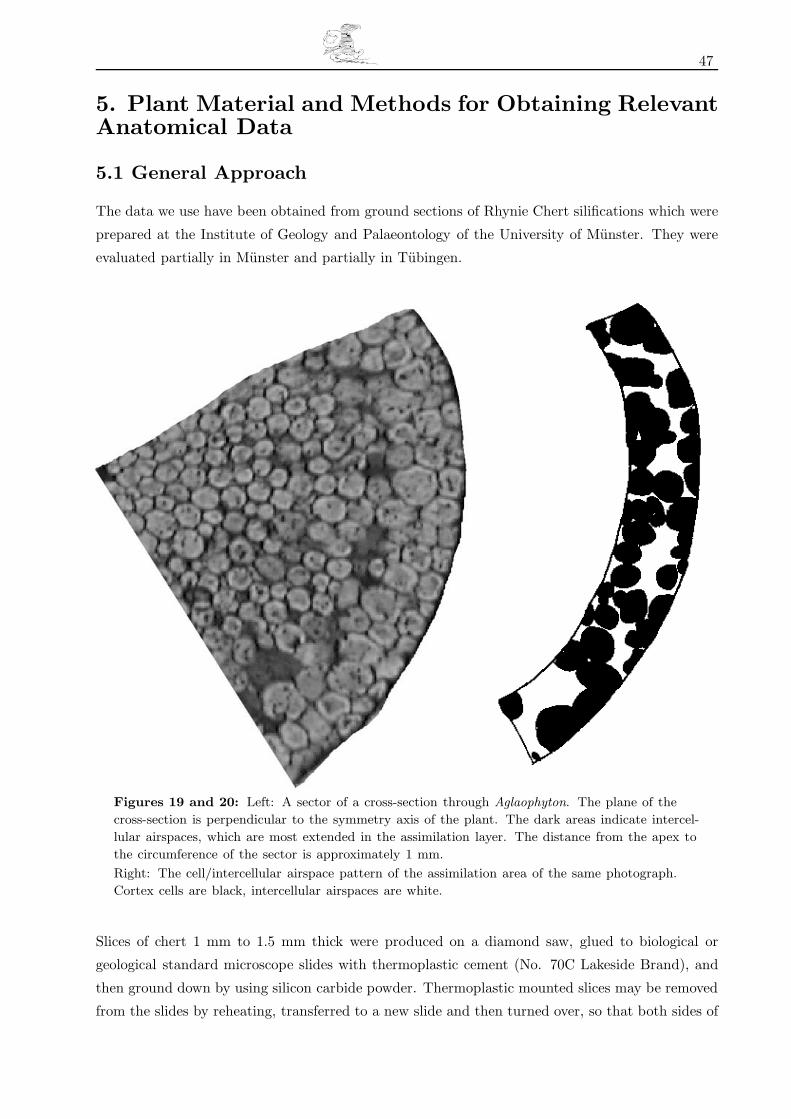
47
5. Plant Material and Methods for Obtaining RelevantAnatomical Data
5.1 General Approach
The data we use have been obtained from ground sections of Rhynie Chert silifications which were
prepared at the Institute of Geology and Palaeontology of the University of Munster. They were
evaluated partially in Munster and partially in Tubingen.
Figures 19 and 20: Left: A sector of a cross-section through Aglaophyton. The plane of the
cross-section is perpendicular to the symmetry axis of the plant. The dark areas indicate intercel-
lular airspaces, which are most extended in the assimilation layer. The distance from the apex to
the circumference of the sector is approximately 1 mm.
Right: The cell/intercellular airspace pattern of the assimilation area of the same photograph.
Cortex cells are black, intercellular airspaces are white.
Slices of chert 1 mm to 1.5 mm thick were produced on a diamond saw, glued to biological or
geological standard microscope slides with thermoplastic cement (No. 70C Lakeside Brand), and
then ground down by using silicon carbide powder. Thermoplastic mounted slices may be removed
from the slides by reheating, transferred to a new slide and then turned over, so that both sides of

48
the slices may be ground down to the plane desired. The ultimate thickness of the slices depends
on the nature of the material (50 µm to 100 µm for higher magnifications and several 100 µm for
overviews, e.g. of epidermal patterns). They are viewed by transmitted or reflected light without
a cover slip, but with a film of oil for all objectives.
Measurements of linear dimensions like the depth of stomatal pores, the length of their long and
short axes, and similar quantities for the hypodermal layer were carried out either with an ocular
micrometer or from photographs. The thicknesses of the layers were determined from photographs
like the one in Figure 9 (in Section 2) or in Figure 19, which allow a clear identification of stomata,
hypodermal channels, cells and intercellular airspaces.
Porosities were obtained by copying the cell/intercellular airspace pattern of the assimilation area
from photographs as in Figure 19 onto transparent overlays. A typical result is depicted as Figure
20. These overlays were scanned and evaluated with the image processing software OPTIMAS,
which determines the total area of the figure and the percentage of its black and white portions.
The white areas in Figure 20 represent the intercellular airspaces. Therefore, in the case of Figure
19, the porosity nas is given as the fraction of the white areas of the total area. The justification
for this method was outlined in Section 4.4.
5.2 Numerical Values
The numerical values of the parameters which were calculated in a general way in Section 4 are
listed in the Tables below. They include
(i) anatomical properties (Table 1),
(ii) environmental parameters (Table 2) and
(iii) biochemical and physiological parameters (Table 3).
The anatomical properties are derived from thin sections of fossilized specimen of Aglaophyton
major and Rhynia gwynne-vaughanii (see Section 5.1).
The environmental parameters represent a Lower Devonian atmosphere as described in the liter-
ature (Berner, 1997), an arbitrary chosen atmospheric humidity and wind velocity and a typical
value for the irradiance I for moderate latitudes.
In the case of the biochemical and physiological parameters, values from extant C3 plants are
applied (data compiled from Harley & Sharkey, 1991, Harley et al., 1992 and Wullschleger, 1993).
The value for gliq is from Parkhurst & Mott, 1990. The chosen parameters for Vmax and Jmax are
at the lower range for modern plants (Wullschleger, 1993). Corresponding values can be found in,
for example, fern leaves or conifer needles.
Two remarks concerning the photosynthetic parameters Vmax and Jmax and the irradiation I are
appropriate:
(i) Values for Vmax and Jmax found in the literature cannot be used in our model without pre-
caution, because we do not adopt the widespread convention to relate the fluxes Vmax and

49
Jmax to a (in our case particularly) fictitious “leaf area” far away from the chloroplasts, where
the carbon dioxide molecules are actually processed. Although it is standard in the field of
plant physiology, it is nonetheless a puzzling measure12. This is made worse by the fact, that
by relating Vmax and Jmax to the leaf surface area these biochemical constants become in-
termingled with the anatomical ratio (Ames/A) of the (total) surface of all mesophyll cells to
the (total) leaf area. (In modern leaves, mesophyll cells are the equivalent of the outer cortex
cells of rhyniophytic plants.)13. Thus, biochemical constants, which should not vary very much
among species, get mixed up with the species-specific morphology. In our case this is especially
unfortunate, because (i), (Ames/A)-values for extant mesophytic plants, which are the prin-
cipal source of (modern) data, differ considerably from the (Ames/A)-values of rhyniophytic
plants, and, (ii) we use photosynthetic data from extant conifer needles 14.
In order to make values from the literature applicable to rhyniophytic plants we redefine Vmax
and Jmax according to the following “local” definition: a flux (or a current density) is (i),
the number of particles, which cross a small surface element during a small temporal interval,
divided by (ii), the area of the surface element they are actually crossing, and divided by (iii),
the time interval which actually elapsed during their passage.
Now we connect the usual convention with this “local” definition: Consider a (total) current
Itot [mol/s] of molecules streaming into (or out of) the chloroplasts of one leaf under stationary
conditions. Achl, Ames and A shall denote the total areas of all chloroplasts, of all mesophyll
cells and of the total leaf surface (i.e. area of upper side of leaf plus area of lower side),
respectively. If the corresponding fluxes — the symbol j stands for either Vmax or Jmax — are
defined by
jchl :=Itot
Achljmes :=
Itot
Amesj :=
Itot
A(5.2)
elimination of Itot from (5.2) results in
12 The usual convention is of course convenient for experimentalists performing measurements with plants
showing foliage leaves. But from the viewpoint of a theorist, it is absurd. Consider a mid-european
cookery-book, which makes extensive use of hen’s eggs, but gives the number of hen’s eggs used in the
recipes not in numbers of hen’s eggs but rather as fractions of ostrich eggs or multiples of colibri eggs.
Even if the book provides an appendix with conversion tables between typical volumes and typical
percentages of white and yellow of the three egg species, it is predictable that many dishes will end
up as mathematical and culinary desasters.13 Still worse, some authors relate Vmax and Jmax to the “projected leaf area”, which implies in the
case of conifer needles that the specific shape of the needles, the details of the projection procedure
and perhaps even contributions from statistics enter the values of Vmax and Jmax, too.14 In our model, the ratio (Ames/A) is not explicitly used, it is rather hidden in other morphological
parameters. If desired, it can be calculated from values in Table 1 via the equation
Ames
A=(
aas
vas
)(1 − nas)
r12 − r0
2
2R(5.1)
with the results (Ames/A) = 5.3 (Aglaophyton) and (Ames/A) = 2.2 (Rhynia).
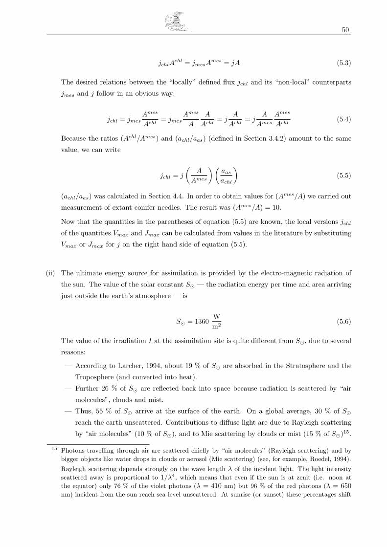
50
jchlAchl = jmesA
mes = jA (5.3)
The desired relations between the “locally” defined flux jchl and its “non-local” counterparts
jmes and j follow in an obvious way:
jchl = jmesAmes
Achl= jmes
Ames
A
A
Achl= j
A
Achl= j
A
Ames
Ames
Achl(5.4)
Because the ratios (Achl/Ames) and (achl/aas) (defined in Section 3.4.2) amount to the same
value, we can write
jchl = j
(A
Ames
)(aas
achl
)(5.5)
(achl/aas) was calculated in Section 4.4. In order to obtain values for (Ames/A) we carried out
measurement of extant conifer needles. The result was (Ames/A) = 10.
Now that the quantities in the parentheses of equation (5.5) are known, the local versions jchl
of the quantities Vmax and Jmax can be calculated from values in the literature by substituting
Vmax or Jmax for j on the right hand side of equation (5.5).
(ii) The ultimate energy source for assimilation is provided by the electro-magnetic radiation of
the sun. The value of the solar constant S� — the radiation energy per time and area arriving
just outside the earth’s atmosphere — is
S� = 1360Wm2
(5.6)
The value of the irradiation I at the assimilation site is quite different from S�, due to several
reasons:
— According to Larcher, 1994, about 19 % of S� are absorbed in the Stratosphere and the
Troposphere (and converted into heat).
— Further 26 % of S� are reflected back into space because radiation is scattered by “air
molecules”, clouds and mist.
— Thus, 55 % of S� arrive at the surface of the earth. On a global average, 30 % of S�reach the earth unscattered. Contributions to diffuse light are due to Rayleigh scattering
by “air molecules” (10 % of S�), and to Mie scattering by clouds or mist (15 % of S�)15.
15 Photons travelling through air are scattered chiefly by “air molecules” (Rayleigh scattering) and by
bigger objects like water drops in clouds or aerosol (Mie scattering) (see, for example, Roedel, 1994).
Rayleigh scattering depends strongly on the wave length λ of the incident light. The light intensity
scattered away is proportional to 1/λ4, which means that even if the sun is at zenit (i.e. noon at
the equator) only 76 % of the violet photons (λ = 410 nm) but 96 % of the red photons (λ = 650nm) incident from the sun reach sea level unscattered. At sunrise (or sunset) these percentages shift

51
It should be noted, that these percentages are valid only on a global scale. Locally, they
are apt to wide variations, depending on local weather conditions and air pollution.
— The hitherto given radiation rates encompass the entire electro-magnetic spectrum. Pho-
tosynthesis, however, uses only radiation with wavelengths in the range 380 nm ≤ λ ≤710 nm. On an average, 45 % – 50 % of the radiation from the sun fall into that range.
Here, we use the value 45 %.
— Thus, if the sun is in the zenit (i.e. vertically above a horizontally oriented area on
the surface of the earth), the photosynthetically active radiation impinging on this area
consists of a term Idirect⊕ , describing the direct (unscattered) radiation, and of a term
Idiffuse⊕ , describing the diffuse radiation, which has been scattered by air molecules, clouds
and mist and was not reflected back into space:
Idirect⊕ = 0.2454S� = 334
Wm2
� 1502µmolm2s
(5.7)
Idiffuse⊕ = 0.2045S� = 278
Wm2
� 1251µmolm2s
(5.8)
where we have used the relation 1 W/m2 � 4.5 µmol/m2s to convert radiation energy to
number of photons16.
— Due to their axially symmetric shape rhyniophytic plants can exploit radiation coming
from the sun only partially. The plant tissue of an upright standing telome of radius R
and length (i.e. height) L absorbs all photons which impinge on the rectangle resulting
from projecting the telome onto a plane situated perpendicular to the direction of the
incoming light rays. If the sun is elevated above the horizon by an angle Θ, the area of
this rectangle is given by 2R × L × cos Θ. Therefore, the number of unscattered photons
which are absorbed per unit time by the whole telome is 2R L cos Θ × Idirect⊕ .
The rate of photons which were originally (i.e. outside the atmosphere) directed onto the
telome but became scattered away from their straight path while traversing the atmosphere
to 0.0065 % (violet photons) and 21 % (red photons). Reflecting upon these ratios for a moment, it
should become clear, that the blueness of the sky, the redness of the sunset, the waneness of the winter
sun, and the ease of sunburning at midday in summer are all consequences of the 1/λ4 dependance
of Rayleigh scattering in the atmosphere (Jackson, 1975).
Mie scattering is proportional only to 1/λ. Nonetheless, in clear weather, it extracts about the same
percentage of blue photons from incident light as Rayleigh scattering, but high humidity or clouds
increase the amount of diffuse light considerably.16 This conversion is necessarily an approximate one, since it depends on the energy distribution among
the photons, which form the radiation. For photons of a fixed wavelength (i.e. fixed energy) the
following relations hold:
1 mol photons � 1.8 × 10⁵ J (for red photons, λ = 650 nm)
1 mol photons � 2.7 × 10⁵ J (for violet photons, λ = 450 nm)
The value 1 W/m2 � 4.5 µmol/m2s is obtained by taking the (unweighted) average over red and
violet photons.

52
is given by 2R L cos Θ × Idiffuse⊕ . Since they represent, by assumption, diffuse light, we
have to distribute them uniformly onto the entire telome surface area 2πR L. The result
is
IdiffuseΘ :=
2R L cos Θ2πR L
Idiffuse⊕ =
cos Θπ
Idiffuse⊕ = cos Θ × 398
µmolm2s
(5.9)
Note, that at noon local time the angle Θ is connected with the geographic latitude B of
a location via Θ = 90 ◦ − B.
— A correct desription of the situation ought to take into account that the irradiance is
constant (and equal to IdiffuseΘ ) on the shadow side of a telome, but varies on the sunny
side of the telome according to IdiffuseΘ + Idirect
⊕ sin ϕ. (ϕ denotes the angle between (i) the
plane spanned by the telome axis and the straight line connecting the sun and any point on
the telome axis, and (ii) the plane spanned by the telome axis and one of the terminators on
the telome surface. The terminators lie at ϕ = 0 ◦ and ϕ = 180 ◦, the brightest (vertical)
line on the telome surface lies at ϕ = 90 ◦.) Driving accuracy that far would complicate
computations considerably, since it would be tempting to include also effects such as the
movement of chloroplasts in response to varying levels and wavelenghts of the incident
light. (Chloroplasts seem to distribute themselves uniformly across the (inner) surface of
a mesophyll cell, if the incident light is not too intensive. In intense light, however, they
lump together at the bright end of the mesophyll cells. See Augustynowicz & Gabrys,
1999.)
Therefore, and because the cited ratio between direct and diffuse irradiation is valid only
on a global scale (global in a spatial and temporal sense), we ignore these effects and
proceed with the averaging process one step further. That is, we distribute also the
unscattered component Idirect⊕ of the impinging light evenly onto the telome surface. The
result is similar to the one derived for the diffuse light
IdirectΘ :=
2R L cos Θ2πR L
Idirect⊕ =
cos Θπ
Idirect⊕ = cos Θ × 478
µmolm2s
(5.10)
It should be noted, that the averaging procedure for Idirect⊕ leads to erraneous results even
without the effect of chloroplast movement, because assimilation depends either not at all
(if limited by Rubisco activity, equation (3.34)) or in a non-linear manner (if limited by
electron transport, equations (3.35) and (3.36)) on the irradiance. Consider a situation
in which the chloroplasts on the sunny side of the telome act in saturated photosynthesis
mode, while their counterparts on the shadow side are idle. The combined assimilation rate
of all chloroplasts in this situation will, in general, be different from the total assimilation
rate of all chloroplasts of the whole telome, if they act under an averaged irradiance and
are photosynthesizing in linear mode.
— Combining equations (5.9) and (5.10) we arrive at
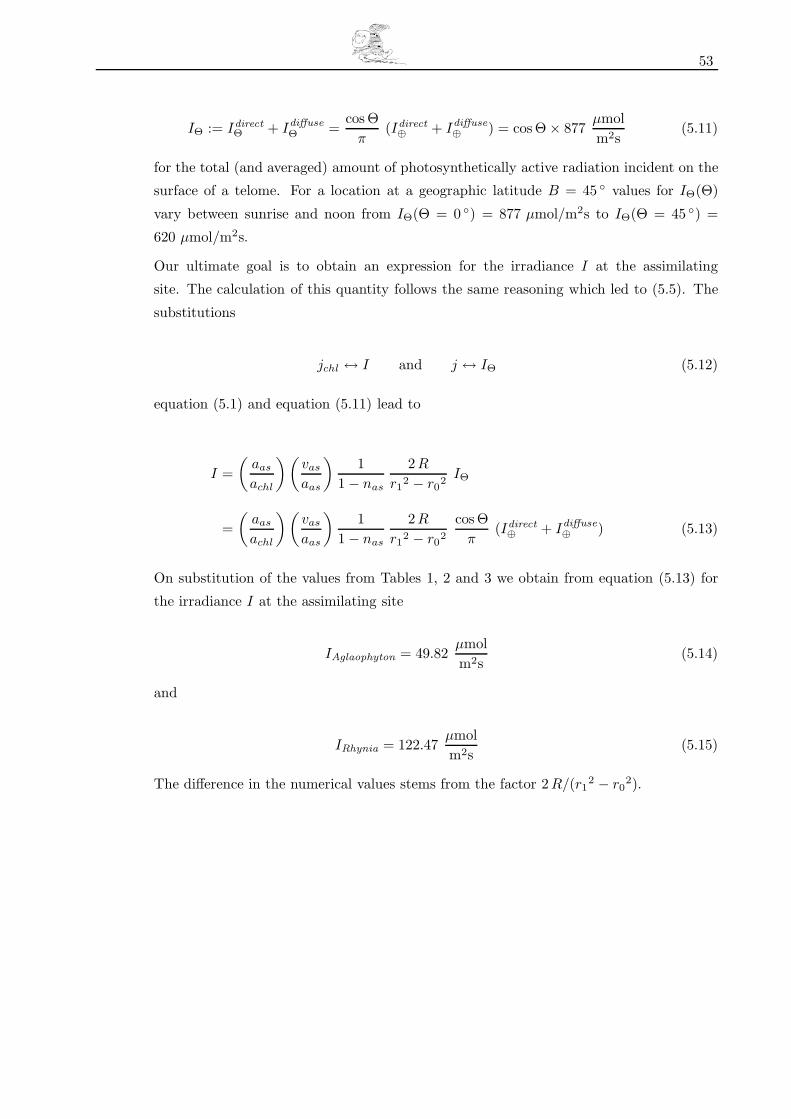
53
IΘ := IdirectΘ + Idiffuse
Θ =cos Θ
π(Idirect
⊕ + Idiffuse⊕ ) = cos Θ × 877
µmolm2s
(5.11)
for the total (and averaged) amount of photosynthetically active radiation incident on the
surface of a telome. For a location at a geographic latitude B = 45 ◦ values for IΘ(Θ)
vary between sunrise and noon from IΘ(Θ = 0 ◦) = 877 µmol/m2s to IΘ(Θ = 45 ◦) =
620 µmol/m2s.
Our ultimate goal is to obtain an expression for the irradiance I at the assimilating
site. The calculation of this quantity follows the same reasoning which led to (5.5). The
substitutions
jchl ↔ I and j ↔ IΘ (5.12)
equation (5.1) and equation (5.11) lead to
I =(
aas
achl
)(vas
aas
)1
1 − nas
2R
r12 − r0
2IΘ
=(
aas
achl
)(vas
aas
)1
1 − nas
2R
r12 − r0
2
cos Θπ
(Idirect⊕ + Idiffuse
⊕ ) (5.13)
On substitution of the values from Tables 1, 2 and 3 we obtain from equation (5.13) for
the irradiance I at the assimilating site
IAglaophyton = 49.82µmolm2s
(5.14)
and
IRhynia = 122.47µmolm2s
(5.15)
The difference in the numerical values stems from the factor 2 R/(r12 − r0
2).
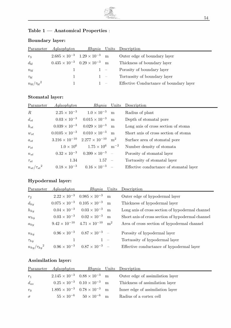
54
Table 1 — Anatomical Properties :
Boundary layer:
Parameter Aglaophyton Rhynia Units Description
r3 2.685 × 10⁻³ 1.29 × 10⁻³ m Outer edge of boundary layer
dbl 0.435 × 10⁻³ 0.29 × 10⁻³ m Thickness of boundary layer
nbl 1 1 – Porosity of boundary layer
τbl 1 1 – Tortuosity of boundary layer
nbl/τbl2 1 1 – Effective Conductance of boundary layer
Stomatal layer:
Parameter Aglaophyton Rhynia Units Description
R 2.25 × 10⁻³ 1.0 × 10⁻³ m Radius of plant
dst 0.03 × 10⁻³ 0.015 × 10⁻³ m Depth of stomatal pore
hst 0.039 × 10⁻³ 0.029 × 10⁻³ m Long axis of cross section of stoma
wst 0.0105 × 10⁻³ 0.010 × 10⁻³ m Short axis of cross section of stoma
ast 3.216 × 10⁻¹⁰ 2.277 × 10⁻¹⁰ m2 Surface area of stomatal pore
νst 1.0 × 10⁶ 1.75 × 10⁶ m−2 Number density of stomata
nst 0.32 × 10⁻³ 0.399 × 10⁻³ – Porosity of stomatal layer
τst 1.34 1.57 – Tortuosity of stomatal layer
nst/τst2 0.18 × 10⁻³ 0.16 × 10⁻³ – Effective conductance of stomatal layer
Hypodermal layer:
Parameter Aglaophyton Rhynia Units Description
r2 2.22 × 10⁻³ 0.985 × 10⁻³ m Outer edge of hypodermal layer
dhy 0.075 × 10⁻³ 0.105 × 10⁻³ m Thickness of hypodermal layer
hhy 0.04 × 10⁻³ 0.03 × 10⁻³ m Long axis of cross section of hypodermal channel
why 0.03 × 10⁻³ 0.02 × 10⁻³ m Short axis of cross section of hypodermal channel
ahy 9.42 × 10⁻¹⁰ 4.71 × 10⁻¹⁰ m2 Area of cross section of hypodermal channel
nhy 0.96 × 10⁻³ 0.87 × 10⁻³ – Porosity of hypodermal layer
τhy 1 1 – Tortuosity of hypodermal layer
nhy/τhy2 0.96 × 10⁻³ 0.87 × 10⁻³ – Effective conductance of hypodermal layer
Assimilation layer:
Parameter Aglaophyton Rhynia Units Description
r1 2.145 × 10⁻³ 0.88 × 10⁻³ m Outer edge of assimilation layer
das 0.25 × 10⁻³ 0.10 × 10⁻³ m Thickness of assimilation layer
r0 1.895 × 10⁻³ 0.78 × 10⁻³ m Inner edge of assimilation layer
σ 55 × 10−6 50 × 10−6 m Radius of a cortex cell
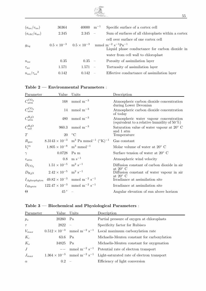
55
(aas/vas) 36364 40000 m−1 Specific surface of a cortex cell
(achl/aas) 2.345 2.345 – Sum of surfaces of all chloroplasts within a cortex
cell over surface of one cortex cellgliq 0.5 × 10⁻³ 0.5 × 10⁻³ mmol m−2 s−1Pa−1
Liquid phase conductance for carbon dioxide in
water from cell wall to chloroplast
nas 0.35 0.35 – Porosity of assimilation layer
τas 1.571 1.571 – Tortuosity of assimilation layer
nas/τas2 0.142 0.142 – Effective conductance of assimilation layer
Table 2 — Environmental Parameters :
Parameter Value Units Description
CCO2atm 168 mmol m−3 Atmospheric carbon dioxide concentration
during Lower DevonianCCO2
atm 14 mmol m−3 Atmospheric carbon dioxide concentrationof today
CH2Oatm 480 mmol m−3 Atmospheric water vapour concentration
(equivalent to a relative humidity of 50 %)CH2O
sat 960.3 mmol m−3 Saturation value of water vapour at 20◦ Cand 1 atm
T 20 ◦C Temperature
Rgas 8.3143 × 10⁻³ m3 Pa mmol−1 (◦K)−1 Gas constant
V ml 1.805 × 10⁻⁸ m3 mmol−1 Molar volume of water at 20◦ C
γ 0.0728 Pa m Surface tension of water at 20◦ C
vatm 0.8 m s−1 Atmospheric wind velocity
DCO21.51 × 10−5 m2 s−1 Diffusion constant of carbon dioxide in air
at 20◦ CDH2O 2.42 × 10⁻⁵ m2 s−1 Diffusion constant of water vapour in air
at 20◦ CIAglaophyton 49.82 × 10⁻³ mmol m−2 s−1 Irradiance at assimilation site
IRhynia 122.47 × 10⁻³ mmol m−2 s−1 Irradiance at assimilation site
Θ 45 ◦ – Angular elevation of sun above horizon
Table 3 — Biochemical and Physiological Parameters :
Parameter Value Units Description
po 20260 Pa Partial pressure of oxygen at chloroplasts
τ 2822 – Specificity factor for Rubisco
Vmax 0.512 × 10⁻³ mmol m−2 s−1 Local maximum carboxylation rate
Kc 63.6 Pa Michaelis-Menten constant for carboxylation
Ko 34825 Pa Michaelis-Menten constant for oxygenation
J −− mmol m−2 s−1 Potential rate of electron transport
Jmax 1.364 × 10⁻³ mmol m−2 s−1 Light-saturated rate of electron transport
α 0.2 – Efficiency of light conversion

56
6. Results
The most direct results of our calculations are the solutions (3.72) and (3.73) of the differential
equation (3.71) and of Fick’s first law (3.1) — the local concentrations of carbon dioxide and of
water vapour, and the corresponding fluxes.
Most interesting for application in fields as plant physiology, ecophysiology or climatology are the
assimilation rate jCO2(R) and the transpiration rate jH2O(R), and especially the dependance of
these rates from the variables, which “define” the plant and its environment. These can be grouped
into three categories:
(i) Five variables defining the environmental conditions, i.e. the atmospheric carbon dioxide
and water vapour concentrations CCO2atm and CH2O
atm , the atmospheric wind velocity vatm, the
irradiance I of photosynthetic active electromagnetic radiation and the temperature T 17.
(ii) Twenty variables defining the plant anatomy, i.e. the axis radius R, the thicknesses dst, dhy
and das of the various layers18, the porosities dbl, dst, dhy and das and the tortuosities nbl, nst,
nhy and nas, the number density of stomata νst, the long and short axes of the cross sections
of the stomata and the hypodermal channels hst, hhy, wst and why, respectively, the radius of
a cortex cell σ, the sum of surfaces of all chloroplasts within a cortex cell over the surface of
one cortex cell (achl/aas) and the liquid phase conductance for carbon dioxide in water from
cell wall to chloroplast gliq.
(iii) Eight variables describing the physiological and biochemical behaviour, i.e. the partial pres-
sure of oxygen at chloroplasts po, the specificity factor for Rubisco τ , the local maximum
carboxylation rate Vmax, the light-saturated rate of electron transport Jmax, the Michaelis-
Menten constants for carboxylation Kc and for oxygenation Ko, the potential rate of electron
transport J and the efficiency of light conversion α.
The most straightforward (and most reliable) approach to investigate the behaviour of the assimila-
tion and transpiration rates under variation of the 33 variables19 cited in (i), (ii) and (iii), would be
to write down jCO2(R) and jH2O(R) as functions of these variables and to determine their extrema,
17 Although the temperature T emerges in various formulas, in its present state, our model does not
simulate a true temperature dependance, because
— “constants” like the diffusion constants, the Michaelis-Menten constants or the molar volume of
water are in reality — but not in the framework of our model — functions of T . They are, at
least as fitted curves, available from the literature,
— a worthwhile extension of the model should incorporate the temperature not only as an “external
parameter”, but as a “dynamic variable”. This is a necessary prerequisite for a realistic description
of thermodynamic feedback effects like transpiration. (Transpiration rate is a function of plant
temperature, plant temperature is influenced by the amount of heat needed for transpiration,
etc..)
18 Note that dbl is not an independent parameter, it is rather a function of the atmospheric wind velocity
vatm.19 To be more precise, the assimilation rate depends only on 32 variables (not on CH2O
atm ), the transpiration
rate merely on 17 of the 33 variables mentioned, chiefly because it is not involved in photosynthesis.
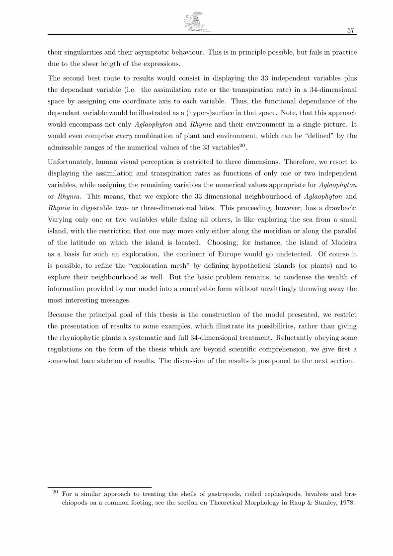
57
their singularities and their asymptotic behaviour. This is in principle possible, but fails in practice
due to the sheer length of the expressions.
The second best route to results would consist in displaying the 33 independent variables plus
the dependant variable (i.e. the assimilation rate or the transpiration rate) in a 34-dimensional
space by assigning one coordinate axis to each variable. Thus, the functional dependance of the
dependant variable would be illustrated as a (hyper-)surface in that space. Note, that this approach
would encompass not only Aglaophyton and Rhynia and their environment in a single picture. It
would even comprise every combination of plant and environment, which can be “defined” by the
admissable ranges of the numerical values of the 33 variables20.
Unfortunately, human visual perception is restricted to three dimensions. Therefore, we resort to
displaying the assimilation and transpiration rates as functions of only one or two independent
variables, while assigning the remaining variables the numerical values appropriate for Aglaophyton
or Rhynia. This means, that we explore the 33-dimensional neighbourhood of Aglaophyton and
Rhynia in digestable two- or three-dimensional bites. This proceeding, however, has a drawback:
Varying only one or two variables while fixing all others, is like exploring the sea from a small
island, with the restriction that one may move only either along the meridian or along the parallel
of the latitude on which the island is located. Choosing, for instance, the island of Madeira
as a basis for such an exploration, the continent of Europe would go undetected. Of course it
is possible, to refine the “exploration mesh” by defining hypothetical islands (or plants) and to
explore their neighbourhood as well. But the basic problem remains, to condense the wealth of
information provided by our model into a conceivable form without unwittingly throwing away the
most interesting messages.
Because the principal goal of this thesis is the construction of the model presented, we restrict
the presentation of results to some examples, which illustrate its possibilities, rather than giving
the rhyniophytic plants a systematic and full 34-dimensional treatment. Reluctantly obeying some
regulations on the form of the thesis which are beyond scientific comprehension, we give first a
somewhat bare skeleton of results. The discussion of the results is postponed to the next section.
20 For a similar approach to treating the shells of gastropods, coiled cephalopods, bivalves and bra-
chiopods on a common footing, see the section on Theoretical Morphology in Raup & Stanley, 1978.
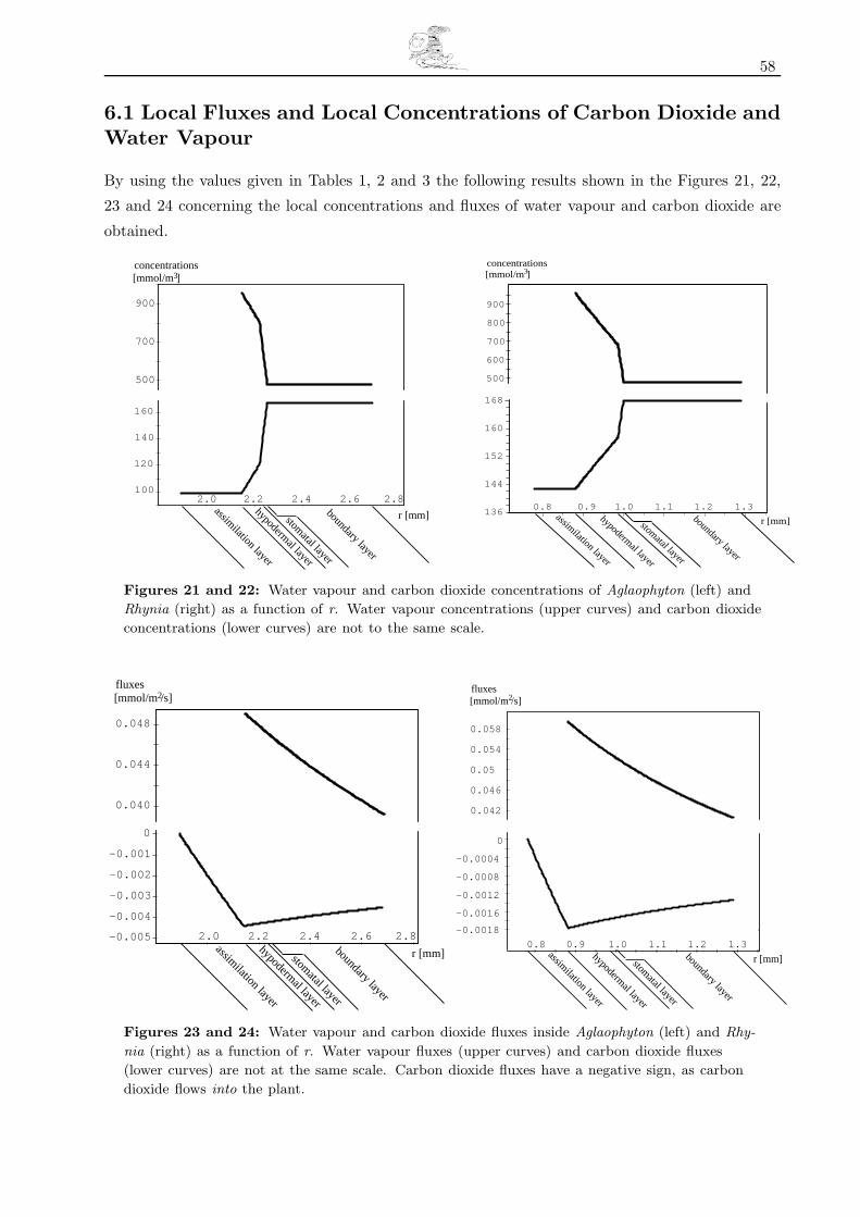
58
6.1 Local Fluxes and Local Concentrations of Carbon Dioxide andWater Vapour
By using the values given in Tables 1, 2 and 3 the following results shown in the Figures 21, 22,
23 and 24 concerning the local concentrations and fluxes of water vapour and carbon dioxide are
obtained.
500
700
900
2.0 2.2 2.4 2.6 2.8
concentrations[mmol/m ]3
r [mm]assimilation layer
hypodermal layer
stomatal layer
boundary layer
100
120
140
160
concentrations[mmol/m ]3
r [mm]assimilation layer
hypodermal layer
stomatal layer
boundary layer
0.8 0.9 1.0 1.1 1.2 1.3
500
600
700
800
900
144
152
160
168
136
Figures 21 and 22: Water vapour and carbon dioxide concentrations of Aglaophyton (left) and
Rhynia (right) as a function of r. Water vapour concentrations (upper curves) and carbon dioxide
concentrations (lower curves) are not to the same scale.
0.040
0.044
0.048
2.0 2.2 2.4 2.6 2.8
r [mm]assimilation layer
hypodermal layer
stomatal layer
boundary layer
fluxes[mmol/m /s]2
-0.004
-0.003
-0.002
-0.001
0
-0.005
fluxes[mmol/m /s]2
r [mm]assimilation layer
hypodermal layer
stomatal layer
boundary layer
0.8 0.9 1.0 1.1 1.2 1.3
0.042
0.046
0.05
0.054
0.058
-0.0018
-0.0016
-0.0012
-0.0008
-0.0004
0
Figures 23 and 24: Water vapour and carbon dioxide fluxes inside Aglaophyton (left) and Rhy-
nia (right) as a function of r. Water vapour fluxes (upper curves) and carbon dioxide fluxes
(lower curves) are not at the same scale. Carbon dioxide fluxes have a negative sign, as carbon
dioxide flows into the plant.
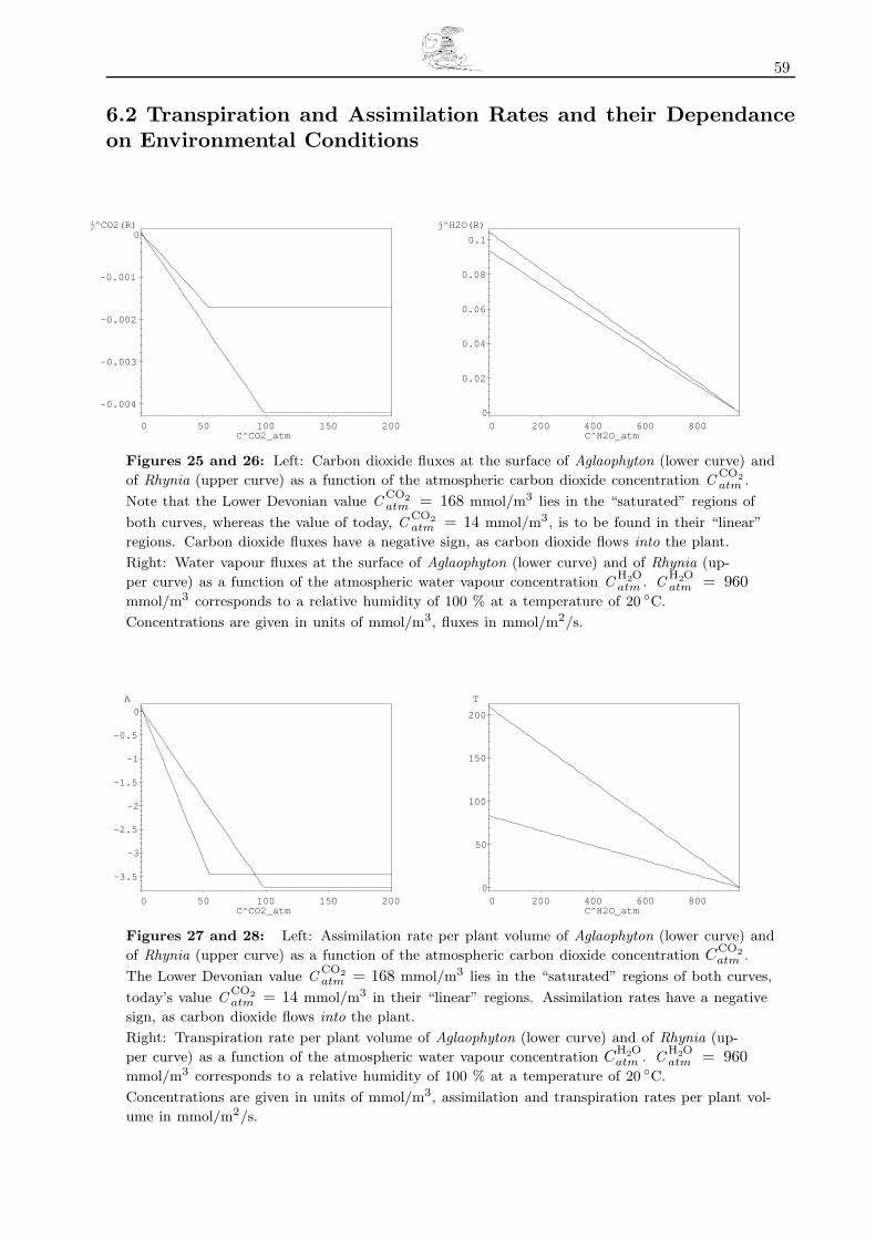
59
6.2 Transpiration and Assimilation Rates and their Dependanceon Environmental Conditions
-0.004
-0.003
-0.002
-0.001
j^CO2(R)0
0 50 100 150 200C^CO2_atm
0
0.02
0.04
0.06
0.08
0.1
j^H2O(R)
0 200 400 600 800C^H2O_atm
Figures 25 and 26: Left: Carbon dioxide fluxes at the surface of Aglaophyton (lower curve) and
of Rhynia (upper curve) as a function of the atmospheric carbon dioxide concentration CCO2atm .
Note that the Lower Devonian value CCO2atm = 168 mmol/m3 lies in the “saturated” regions of
both curves, whereas the value of today, CCO2atm = 14 mmol/m3, is to be found in their “linear”
regions. Carbon dioxide fluxes have a negative sign, as carbon dioxide flows into the plant.
Right: Water vapour fluxes at the surface of Aglaophyton (lower curve) and of Rhynia (up-
per curve) as a function of the atmospheric water vapour concentration CH2Oatm . C
H2Oatm = 960
mmol/m3 corresponds to a relative humidity of 100 % at a temperature of 20 ◦C.
Concentrations are given in units of mmol/m3, fluxes in mmol/m2/s.
-3.5
-3
-2.5
-2
-1.5
-1
-0.5
0A
0 50 100 150 200C^CO2_atm
0
50
100
150
200
T
0 200 400 600 800C^H2O_atm
Figures 27 and 28: Left: Assimilation rate per plant volume of Aglaophyton (lower curve) and
of Rhynia (upper curve) as a function of the atmospheric carbon dioxide concentration CCO2atm .
The Lower Devonian value CCO2atm = 168 mmol/m3 lies in the “saturated” regions of both curves,
today’s value CCO2atm = 14 mmol/m3 in their “linear” regions. Assimilation rates have a negative
sign, as carbon dioxide flows into the plant.
Right: Transpiration rate per plant volume of Aglaophyton (lower curve) and of Rhynia (up-
per curve) as a function of the atmospheric water vapour concentration CH2Oatm . C
H2Oatm = 960
mmol/m3 corresponds to a relative humidity of 100 % at a temperature of 20 ◦C.
Concentrations are given in units of mmol/m3, assimilation and transpiration rates per plant vol-
ume in mmol/m2/s.
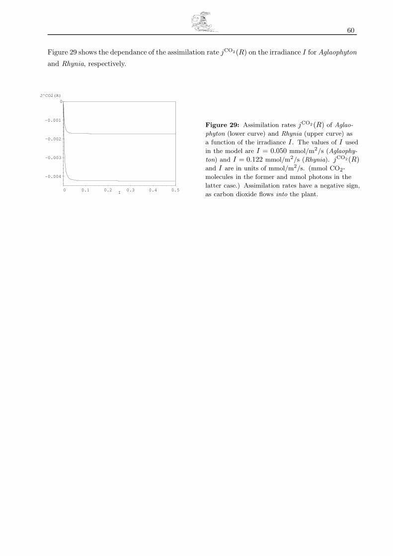
60
Figure 29 shows the dependance of the assimilation rate jCO2(R) on the irradiance I for Aglaophyton
and Rhynia, respectively.
-0.004
-0.003
-0.002
-0.001
0J^CO2(R)
0 0.1 0.2 0.3 0.4 0.5I
Figure 29: Assimilation rates jCO2(R) of Aglao-
phyton (lower curve) and Rhynia (upper curve) as
a function of the irradiance I . The values of I used
in the model are I = 0.050 mmol/m2/s (Aglaophy-
ton) and I = 0.122 mmol/m2/s (Rhynia). jCO2(R)and I are in units of mmol/m2/s. (mmol CO2-
molecules in the former and mmol photons in the
latter case.) Assimilation rates have a negative sign,
as carbon dioxide flows into the plant.

61
6.3 The Water Use Efficiency and its Dependance on AtmosphericConditions
The water use efficiency (WUE) is defined by
WUE :=number of CO2 molecules fixed per time
number of H2O molecules transpired per time=
|A|T =
|jCO2(R)|jH2O(R)
(6.1)
With the numerical values of Tables 1, 2 and 3 we obtain
WUEAglaophyton = 0.0899 ≈ 45 × WUEextant (6.2)
WUERhynia = 0.0329 ≈ 16 × WUEextant (6.3)
where WUEextant = 0.0020 is a typical average value for extant C3 plants (see, for example, Kramer,
1983).
0200
400600
800C^H2O_atm
20 40 60 80100120140160180200C^CO2_atm
0
0.05
0.10
0.15
0.20
0.25
WUE
Figure 30: Water use effi-
ciency WUE of Aglaophyton (up-
per surface) and Rhynia (lower
surface) as a function of the at-
mospheric carbon dioxide CCO2atm
and water vapour CH2Oatm con-
centrations. Concentrations are
given in units of mmol/m3. In
the scale of the figure, the plane
WUEextant = 0.0020 is identical
to the bottom of the cube.
0
0.02
0.04
0.06
0.08
WUE
0 50 100 150 200C^CO2_atm
Figure 31: Water use efficiency WUE of Aglao-
phyton (upper curve) and Rhynia (lower curve) as
a function of the atmospheric carbon dioxide con-
centration CCO2atm at a water vapour concentration of
CH2Oatm = 480 mmol/m3 (equivalent to a relative hu-
midity of 50 %). Concentrations are given in units
of mmol/m3. During the Lower Devonian, the at-
mospheric carbon dioxide concentration amounted
to about 168 mmol/m3, nowadays it has the value
14 mmol/m3.
Figure 30 displays the water use efficiency as a function of the atmospheric carbon dioxide and of
the water vapour concentrations. Figure 31 is a (vertical) section through Figure 30 at a water
vapour concentration CH2Oatm = 480 mmol/m3 (equivalent to a relative humidity of 50 %).

62
6.4 Dependance of Water Use Efficiency, Transpiration and As-similation Rates on Plant Anatomy
Figure 32 displays the water use efficiency of Aglaophyton (upper surface) and Rhynia (lower surface)
as a function of the stomatal density νst and the thickness dhy of the hypodermal layer.
Figures 33 and 34 show carbon dioxide fluxes jCO2(R) and the water vapour fluxes jH2O(R) at the
surface of Aglaophyton (lower surface) and of Rhynia (upper surface), respectively, as a function of
the stomatal density νst and the thickness dhy of the hypodermal layer.
Figure 35 is the counterpart of Figure 33 for the recent atmospheric carbon dioxide content.
0 5e+006 1e+007 1.5e+007 2e+007
nu_st0.20.40.60.81.0
d_hy
0
0.05
0.10
0.15
0.20
WUE
Figure 32: Water use efficiency
(WUE) of Aglaophyton (upper
surface) and Rhynia (lower sur-
face) as a function of the stom-
atal density νst and the thick-
ness dhy of the hypodermal layer.
The stomatal density is given in
1/m2, the thickness of the hy-
podermal layer in mm. Aglao-
phyton’s actual position in the
(νst, dhy)-plane is at (νst, dhy) =(106/m2, 0.075 mm) Rhynia’s po-
sition is at (νst, dhy) = (1.75 ×10⁶/m2, 0.105 mm)
5e+006 1e+007 1.5e+007 2e+007
nu_st0.20.40.60.81.0
d_hyp
-0.004
-0.003
-0.002
-0.001
0
j^CO2(R)
Figure 33: Carbon dioxide
fluxes j CO2(R) at the surface
of Aglaophyton (lower surface)
and of Rhynia (upper surface)
as a function of the stomatal
density νst and the thickness
dhy of the hypodermal layer.
The stomatal density is given in
1/m2, the thickness of the hy-
podermal layer in mm. j CO2(R)
has units mmol/m3. Aglao-
phyton’s actual position in the
(νst, dhy)-plane is at (νst, dhy) =(106/m2, 0.075 mm) Rhynia’s
position is at (νst, dhy) =(1.75 × 10⁶/m2, 0.105 mm)Note, that carbon dioxide fluxes
have a negative sign.

63
0 5e+006 1e+007 1.5e+007 2e+007
nu_st0.20.40.60.81.0
dhyp
0
0.2
0.4
0.6
0.8
1
j^H2O(R)
Figure 34: Water vapour
fluxes j H2O(R) at the surface
of Aglaophyton (lower surface)
and of Rhynia (upper surface)
as a function of the stomatal
density νst and the thickness
dhy of the hypodermal layer.
The stomatal density is given in
1/m2, the thickness of the hy-
podermal layer in mm. j H2O(R)
has units mmol/m3. Aglao-
phyton’s actual position in the
(νst, dhy)-plane is at (νst, dhy) =(106/m2, 0.075 mm) Rhynia’s
position is at (νst, dhy) =(1.75 × 10⁶/m2, 0.105 mm)
0 5e+006 1e+007 1.5e+007 2e+007
nu_st0.20.40.60.81.0
d_hyp
-0.0016
-0.0014
-0.0012
-0.001
-0.0008
-0.0006
-0.0004
-0.0002
0
j^CO2(R)Figure 35: Carbon dioxide
fluxes j CO2(R) at the surface of
Aglaophyton (lower surface) and of
Rhynia (upper surface) in today’s
atmosphere with CCO2atm = 14
mmol/m3. j CO2(R) is — as in
Figure 33 — a function of the
stomatal density νst and the
thickness dhy of the hypodermal
layer. Values of all other parame-
ters are as in Figure 33.
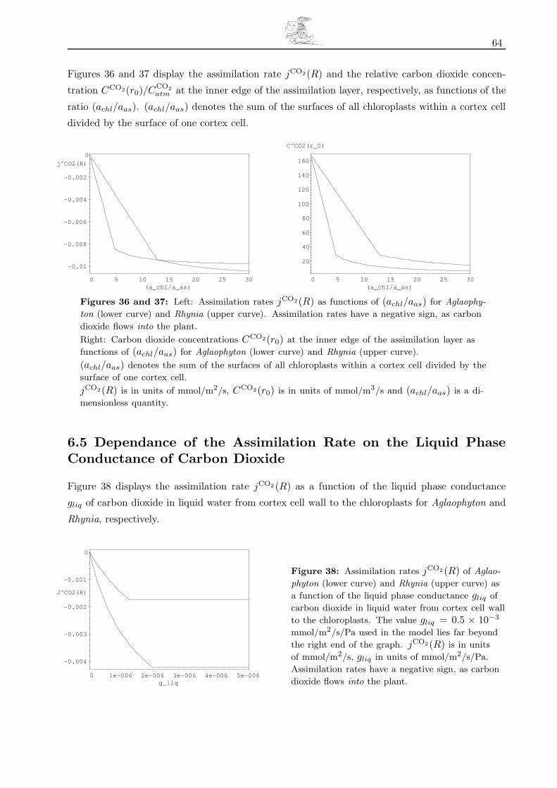
64
Figures 36 and 37 display the assimilation rate jCO2(R) and the relative carbon dioxide concen-
tration CCO2(r0)/CCO2atm at the inner edge of the assimilation layer, respectively, as functions of the
ratio (achl/aas). (achl/aas) denotes the sum of the surfaces of all chloroplasts within a cortex cell
divided by the surface of one cortex cell.
-0.01
-0.008
-0.006
-0.004
-0.002
j^CO2(R)0
0 5 10 15 20 25 30(a_chl/a_as)
C^CO2(r_0)
20
40
60
80
100
120
140
160
0 5 10 15 20 25 30(a_chl/a_as)
Figures 36 and 37: Left: Assimilation rates jCO2(R) as functions of (achl/aas) for Aglaophy-
ton (lower curve) and Rhynia (upper curve). Assimilation rates have a negative sign, as carbon
dioxide flows into the plant.
Right: Carbon dioxide concentrations CCO2(r0) at the inner edge of the assimilation layer as
functions of (achl/aas) for Aglaophyton (lower curve) and Rhynia (upper curve).
(achl/aas) denotes the sum of the surfaces of all chloroplasts within a cortex cell divided by the
surface of one cortex cell.
jCO2(R) is in units of mmol/m2/s, CCO2(r0) is in units of mmol/m3/s and (achl/aas) is a di-
mensionless quantity.
6.5 Dependance of the Assimilation Rate on the Liquid PhaseConductance of Carbon Dioxide
Figure 38 displays the assimilation rate jCO2(R) as a function of the liquid phase conductance
gliq of carbon dioxide in liquid water from cortex cell wall to the chloroplasts for Aglaophyton and
Rhynia, respectively.
-0.004
-0.003
-0.002
-0.001
0
J^CO2(R)
0 1e-006 2e-006 3e-006 4e-006 5e-006g_liq
Figure 38: Assimilation rates jCO2(R) of Aglao-
phyton (lower curve) and Rhynia (upper curve) as
a function of the liquid phase conductance gliq of
carbon dioxide in liquid water from cortex cell wall
to the chloroplasts. The value gliq = 0.5 × 10⁻³
mmol/m2/s/Pa used in the model lies far beyond
the right end of the graph. jCO2(R) is in units
of mmol/m2/s, gliq in units of mmol/m2/s/Pa.
Assimilation rates have a negative sign, as carbon
dioxide flows into the plant.

65
6.6 Dependance of the Assimilation Rate on the Specificity Factorfor Rubisco
Figures 39 and 40 display the assimilation rate jCO2(R) and the carbon dioxide concentration
CCO2(r0) at the inner edge of the assimilation layer, respectively, as functions of the specificity
factor τ for Rubisco for Aglaophyton and Rhynia, respectively. For the definition of τ recall equation
(3.38), Section 3.4.1.
-0.004
-0.003
-0.002
-0.001
0
J^CO2(R)
0.001
0 50 100 150 200 250 300τ
100
120
140
160
180
200
C^CO2(r0)
0 50 100 150 200 250 300τ
Figures 39 and 40: Left: Assimilation rates jCO2(R) of Aglaophyton (lower curve) and Rhy-
nia (upper curve) as a function of the specificity factor τ for Rubisco. jCO2(R) is in units of
mmol/m2/s, τ is without dimension. Assimilation rates have a negative sign, as carbon dioxide
flows into the plant.
Right: Carbon dioxide concentration CCO2(r0) at the inner edge of the assimilation layer as func-
tion of the specificity factor τ for Rubisco for Aglaophyton (lower curve) and Rhynia (upper
curve). CCO2(r0) is in units of mmol/m3, τ is without dimension.
The value τ = 2822 used in the model lies far beyond the right end of both graphs.
6.7 Dependance of the Assimilation Rate on the Efficiency of LightConversion
Figure 41 displays the assimilation rate jCO2(R) as a function of the efficiency of light conversion
α for Aglaophyton and Rhynia, respectively.
-0.0040
-0.0035
-0.0030
-0.0025
-0.0020
-0.0015
-0.0010
J^CO2(R)
0 0.2 0.4 0.6 0.8 1α
Figure 41: Assimilation rates jCO2(R) of Aglao-
phyton (lower curve) and Rhynia (upper curve) as
a function of the efficiency of light conversion α.
jCO2(R) is in units of mmol/m2/s, α is without
dimension. The model employs the value α = 0.2.
Assimilation rates have a negative sign, as carbon
dioxide flows into the plant.

66
6.8 Dependance of the Assimilation Rate on Vmax and Jmax
Figures 42 to 45 display the the assimilation rate jCO2(R) as a function of the local maximum
carboxylation rate Vmax and the light-saturated rate of electron transport Jmax for Aglaophyton
and Rhynia, respectively.
00.002
0.0040.006
0.0080.010
0.012
J_max00.001
0.0020.003
0.0040.005V_max
-0.009
-0.007
-0.005
-0.003
-0.001
J^CO2(R)
Ag
0
0.002
0.004
0.006
0.008
0.010
0.012
J_max
00.001 0.002 0.003 0.004 0.005
V_max
00.002
0.0040.006
0.0080.010
0.012J_max
00.001
0.0020.003
0.0040.005V_max
-0.010
-0.008
-0.006
-0.004
-0.002
J^CO2(R)
Rh
0
0.002
0.004
0.006
0.008
0.010
0.012
J_max
00.001 0.002 0.003 0.004 0.005
V_max
Figures 42, 43, 44 and 45: Assimilation rates jCO2(R) of Aglaophyton (upper pictures) and
Rhynia (lower pictures) as functions of the local maximum carboxylation rate Vmax and the light-
saturated rate of electron transport Jmax. All quantities are in units of mmol/m2/s. Assimilation
rates have a negative sign, as carbon dioxide flows into the plant.
Left: Three-dimensional views.
Right: The same pictures displayed as contour plots. The positions of Aglaophyton and Rhynia on
the (Vmax, Jmax)-plane are marked by ‘Ag’ and ‘Rh’, respectively.
Points lying “northeast” of the crossed line fulfill the condition Vmax < J/4, that is, photosynthe-
sis is limited by the maximum rate of carboxylation. On the other hand, for points “southwest”
of the crossed line the condition Vmax > J/4 is valid, that is, photosynthesis is limited by the
light-saturated rate of electron transport.
Intervals between adjacent contour lines amount to �jCO2(R) = 0.0005 mmol/m2/s.
Upper, right picture: The contour line close to ‘Ag’ corresponds to jCO2(R) = −0.00425mmol/m2/s, the one at the top to jCO2(R) = −0.0015 mmol/m2/s, and the one encircling
the “south-east”-corner to jCO2(R) = −0.0095 mmol/m2/s.
Lower, right picture: The contour line close to ‘Rh’ corresponds to jCO2(R) = −0.00175mmol/m2/s, the one at the top to jCO2(R) = −0.0005 mmol/m2/s, and the one encircling
the “south-east”-corner to jCO2(R) = −0.01 mmol/m2/s.

67
7. Discussion
7.1 Local Fluxes and Local Concentrations of Carbon Dioxide andWater Vapour
By using the values given in Tables 1, 2 and 3 the results shown in Figures 23 and 24 concerning
the local fluxes of water vapour and carbon dioxide are obtained.
It is apparent that the fluxes are quite smooth functions of r outside the assimilation layer. This is
to be expected from the plants’ axial symmetry and from the principle of mass conservation, which
forces the fluxes to vary inversely proportional to r wherever sources or sinks are absent. Formally
this result can be derived from the principle of mass conservation (equation (3.4)): In the absence
of sources (i.e. Q = 0) and under stationary conditions (i.e. ∂C/∂t = 0), axial and translatorial
symmetry with respect to the z-axis imply
0 = div�j + Q − ∂C
∂t=
1r
∂(r jr)∂r
(7.1)
where the definition of the divergence, equation (9.6), has been used, too. The last equation is
equivalent to
r jr = const. (7.2)
from which follows
jr =const.
r(7.3)
The local concentrations of water vapour and carbon dioxide plotted in Figures 21 and 22 against r
behave less smoothly than the fluxes, because their gradients dC(r)/dr = −(1/S) j(r) (see equation
(3.5)) are dominated by the factor 1/S which leaps considerably from layer to layer, exhibiting the
following ratios, which are valid both for carbon dioxide and water vapour diffusion:
1/Sbl : 1/Sst : 1/Shy : 1/Sas ≈ 1 : 5560 : 1036 : 7 (Aglaophyton) (7.4)
1/Sbl : 1/Sst : 1/Shy : 1/Sas ≈ 1 : 6166 : 1144 : 7 (Rhynia) (7.5)
This causes steep gradients of both carbon dioxide and water vapour in the stomatal and hypoder-
mal layers, whereas in the boundary layer and — in the case of carbon dioxide — in the assimilation
layer, the concentrations of both gases remain almost constant.
In a Lower Devonian atmosphere with CCO2atm = 168 mmol/m3 and CH2O
atm = 480 mmol/m3, the inter-
cellular carbon dioxide concentrations inside the assimilating tissue amount to about 99 mmol/m3
(Aglaophyton) and 143 mmol/m3 (Rhynia), which are roughly 59 % and 85 % of the external values.
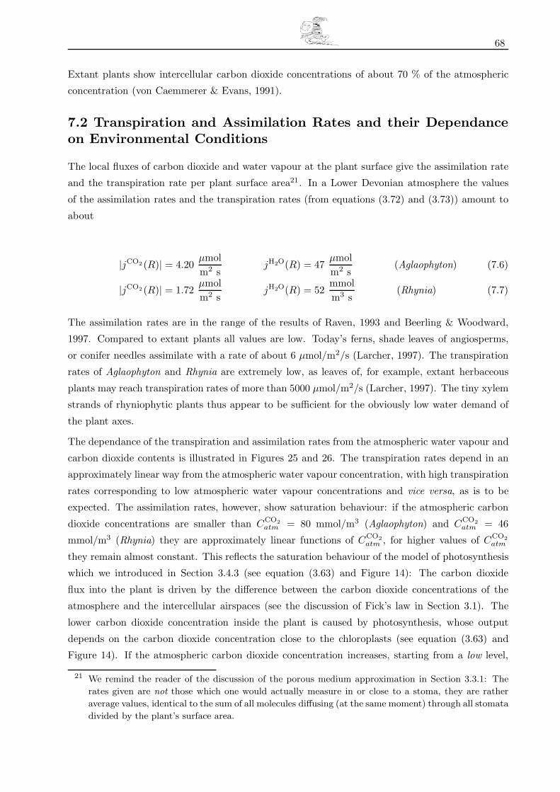
68
Extant plants show intercellular carbon dioxide concentrations of about 70 % of the atmospheric
concentration (von Caemmerer & Evans, 1991).
7.2 Transpiration and Assimilation Rates and their Dependanceon Environmental Conditions
The local fluxes of carbon dioxide and water vapour at the plant surface give the assimilation rate
and the transpiration rate per plant surface area21. In a Lower Devonian atmosphere the values
of the assimilation rates and the transpiration rates (from equations (3.72) and (3.73)) amount to
about
|jCO2(R)| = 4.20µmolm2 s
jH2O(R) = 47µmolm2 s
(Aglaophyton) (7.6)
|jCO2(R)| = 1.72µmolm2 s
jH2O(R) = 52mmolm3 s
(Rhynia) (7.7)
The assimilation rates are in the range of the results of Raven, 1993 and Beerling & Woodward,
1997. Compared to extant plants all values are low. Today’s ferns, shade leaves of angiosperms,
or conifer needles assimilate with a rate of about 6 µmol/m2/s (Larcher, 1997). The transpiration
rates of Aglaophyton and Rhynia are extremely low, as leaves of, for example, extant herbaceous
plants may reach transpiration rates of more than 5000 µmol/m2/s (Larcher, 1997). The tiny xylem
strands of rhyniophytic plants thus appear to be sufficient for the obviously low water demand of
the plant axes.
The dependance of the transpiration and assimilation rates from the atmospheric water vapour and
carbon dioxide contents is illustrated in Figures 25 and 26. The transpiration rates depend in an
approximately linear way from the atmospheric water vapour concentration, with high transpiration
rates corresponding to low atmospheric water vapour concentrations and vice versa, as is to be
expected. The assimilation rates, however, show saturation behaviour: if the atmospheric carbon
dioxide concentrations are smaller than CCO2atm = 80 mmol/m3 (Aglaophyton) and CCO2
atm = 46
mmol/m3 (Rhynia) they are approximately linear functions of CCO2atm , for higher values of CCO2
atm
they remain almost constant. This reflects the saturation behaviour of the model of photosynthesis
which we introduced in Section 3.4.3 (see equation (3.63) and Figure 14): The carbon dioxide
flux into the plant is driven by the difference between the carbon dioxide concentrations of the
atmosphere and the intercellular airspaces (see the discussion of Fick’s law in Section 3.1). The
lower carbon dioxide concentration inside the plant is caused by photosynthesis, whose output
depends on the carbon dioxide concentration close to the chloroplasts (see equation (3.63) and
Figure 14). If the atmospheric carbon dioxide concentration increases, starting from a low level,
21 We remind the reader of the discussion of the porous medium approximation in Section 3.3.1: The
rates given are not those which one would actually measure in or close to a stoma, they are rather
average values, identical to the sum of all molecules diffusing (at the same moment) through all stomata
divided by the plant’s surface area.
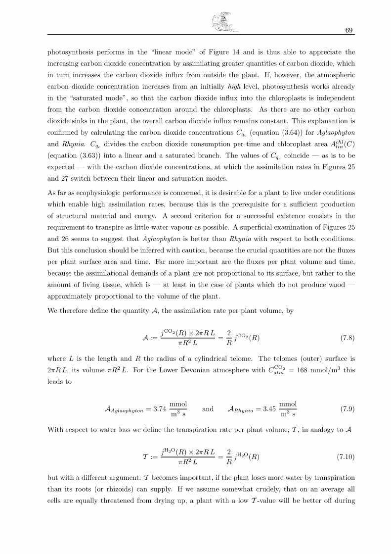
69
photosynthesis performs in the “linear mode” of Figure 14 and is thus able to appreciate the
increasing carbon dioxide concentration by assimilating greater quantities of carbon dioxide, which
in turn increases the carbon dioxide influx from outside the plant. If, however, the atmospheric
carbon dioxide concentration increases from an initially high level, photosynthesis works already
in the “saturated mode”, so that the carbon dioxide influx into the chloroplasts is independent
from the carbon dioxide concentration around the chloroplasts. As there are no other carbon
dioxide sinks in the plant, the overall carbon dioxide influx remains constant. This explanantion is
confirmed by calculating the carbon dioxide concentrations Cqc(equation (3.64)) for Aglaophyton
and Rhynia. Cqcdivides the carbon dioxide consumption per time and chloroplast area Achl
lin(C)
(equation (3.63)) into a linear and a saturated branch. The values of Cqccoincide — as is to be
expected — with the carbon dioxide concentrations, at which the assimilation rates in Figures 25
and 27 switch between their linear and saturation modes.
As far as ecophysiologic performance is concerned, it is desirable for a plant to live under conditions
which enable high assimilation rates, because this is the prerequisite for a sufficient production
of structural material and energy. A second criterion for a successful existence consists in the
requirement to transpire as little water vapour as possible. A superficial examination of Figures 25
and 26 seems to suggest that Aglaophyton is better than Rhynia with respect to both conditions.
But this conclusion should be inferred with caution, because the crucial quantities are not the fluxes
per plant surface area and time. Far more important are the fluxes per plant volume and time,
because the assimilational demands of a plant are not proportional to its surface, but rather to the
amount of living tissue, which is — at least in the case of plants which do not produce wood —
approximately proportional to the volume of the plant.
We therefore define the quantity A, the assimilation rate per plant volume, by
A :=jCO2(R) × 2πR L
πR2 L=
2R
jCO2(R) (7.8)
where L is the length and R the radius of a cylindrical telome. The telomes (outer) surface is
2πR L, its volume πR2 L. For the Lower Devonian atmosphere with CCO2atm = 168 mmol/m3 this
leads to
AAglaophyton = 3.74mmolm3 s
and ARhynia = 3.45mmolm3 s
(7.9)
With respect to water loss we define the transpiration rate per plant volume, T , in analogy to A
T :=jH2O(R) × 2πR L
πR2 L=
2R
jH2O(R) (7.10)
but with a different argument: T becomes important, if the plant loses more water by transpiration
than its roots (or rhizoids) can supply. If we assume somewhat crudely, that on an average all
cells are equally threatened from drying up, a plant with a low T -value will be better off during
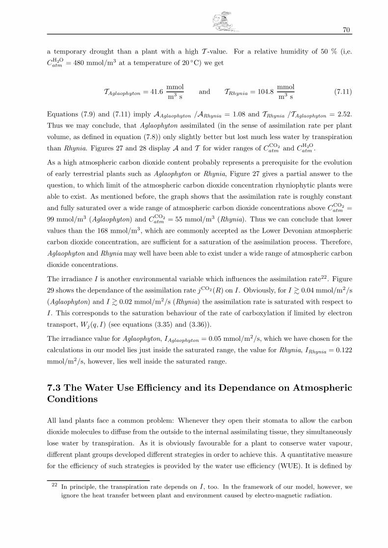
70
a temporary drought than a plant with a high T -value. For a relative humidity of 50 % (i,e.
CH2Oatm = 480 mmol/m3 at a temperature of 20 ◦C) we get
TAglaophyton = 41.6mmolm3 s
and TRhynia = 104.8mmolm3 s
(7.11)
Equations (7.9) and (7.11) imply AAglaophyton /ARhynia = 1.08 and TRhynia /TAglaophyton = 2.52.
Thus we may conclude, that Aglaophyton assimilated (in the sense of assimilation rate per plant
volume, as defined in equation (7.8)) only slightly better but lost much less water by transpiration
than Rhynia. Figures 27 and 28 display A and T for wider ranges of CCO2atm and CH2O
atm .
As a high atmospheric carbon dioxide content probably represents a prerequisite for the evolution
of early terrestrial plants such as Aglaophyton or Rhynia, Figure 27 gives a partial answer to the
question, to which limit of the atmospheric carbon dioxide concentration rhyniophytic plants were
able to exist. As mentioned before, the graph shows that the assimilation rate is roughly constant
and fully saturated over a wide range of atmospheric carbon dioxide concentrations above CCO2atm =
99 mmol/m3 (Aglaophyton) and CCO2atm = 55 mmol/m3 (Rhynia). Thus we can conclude that lower
values than the 168 mmol/m3, which are commonly accepted as the Lower Devonian atmospheric
carbon dioxide concentration, are sufficient for a saturation of the assimilation process. Therefore,
Aglaophyton and Rhynia may well have been able to exist under a wide range of atmospheric carbon
dioxide concentrations.
The irradiance I is another environmental variable which influences the assimilation rate22. Figure
29 shows the dependance of the assimilation rate jCO2(R) on I. Obviously, for I � 0.04 mmol/m2/s
(Aglaophyton) and I � 0.02 mmol/m2/s (Rhynia) the assimilation rate is saturated with respect to
I. This corresponds to the saturation behaviour of the rate of carboxylation if limited by electron
transport, Wj(q, I) (see equations (3.35) and (3.36)).
The irradiance value for Aglaophyton, IAglaophyton = 0.05 mmol/m2/s, which we have chosen for the
calculations in our model lies just inside the saturated range, the value for Rhynia, IRhynia = 0.122
mmol/m2/s, however, lies well inside the saturated range.
7.3 The Water Use Efficiency and its Dependance on AtmosphericConditions
All land plants face a common problem: Whenever they open their stomata to allow the carbon
dioxide molecules to diffuse from the outside to the internal assimilating tissue, they simultaneously
lose water by transpiration. As it is obviously favourable for a plant to conserve water vapour,
different plant groups developed different strategies in order to achieve this. A quantitative measure
for the efficiency of such strategies is provided by the water use efficiency (WUE). It is defined by
22 In principle, the transpiration rate depends on I , too. In the framework of our model, however, we
ignore the heat transfer between plant and environment caused by electro-magnetic radiation.

71
WUE :=number of CO2 molecules fixed per time
number of H2O molecules transpired per time=
|A|T =
|jCO2(R)|jH2O(R)
(7.12)
Taking the water use efficiency as the sole measure for the performance of a plant can be misleading
due to several reasons:
(i) If the transpiration rate T in the denominator of (7.11) becomes close to zero, the fraction
WUE will attain very high values, even if the plants assimilation rate A becomes so small,
that it cannot sustain the plant’s energetic requirements.
(ii) In a real plant, the value of the water use efficiency varies strongly due to temporal stomatal
closure or variations in environmental conditions.
In order to avoid these drawbacks, other long-term parameters — such as the amount of water used
per vegetational period divided by the dry matter produced during that time — are often used.
With the numerical values of Tables 1, 2 and 3 we obtain
WUEAglaophyton = 0.0899 ≈ 45 × WUEextant (7.13)
WUERhynia = 0.0329 ≈ 16 × WUEextant (7.14)
where WUEextant = 0.0020 is a typical average value for extant C3 plants (see, for example, Kramer,
1983). The question arises, whether these relatively high values are due to environmental conditions
— during the Lower Devonian the atmospheric carbon dioxide concentration was twelve times as
high as it is today —, or if the high water use efficiencies calculated in equations (7.13) and (7.14)
are based on the morphological design of rhyniophytic plant axes. A partial answer can be obtained
by consulting Figures 30 and 31. Figure 30 displays the water use efficiency as a function of the
atmospheric carbon dioxide and of the water vapour concentrations. Figure 31 is a (vertical) section
through Figure 30 at a water vapour concentration CH2Oatm = 480 mmol/m3 (equivalent to a relative
humidity of 50 %). The figures show, that for a given water vapour concentration the water use
efficiency is almost constant for a wide range of carbon dioxide concentrations around the Lower
Devonian value of CCO2atm = 168 mmol/m3. It approaches zero more or less linearly, if the carbon
dioxide concentration drops below the values CCO2atm = 99 mmol/m3 (Aglaophyton) and CCO2
atm = 55
mmol/m3 (Rhynia). Under recent atmospheric conditions, Aglaophyton’s and Rhynia’s water use
efficiencies would be
WUEAglaophyton, today = 0.0116 ≈ 5.8 × WUEextant (7.15)
WUERhynia, today = 0.0078 ≈ 3.9 × WUEextant (7.16)
This means that under present day conditions both plants would perform below their respective
optima of water use efficiency, but still more efficient than extant plants. However, we should not

72
ignore the possibility that although the fraction WUE attains high values, the plants assimilation
rate A becomes so small under present day conditions, that it cannot sustain the plant’s energetic
requirements.
Nonetheless, we may conclude from Figure 30 that the water use efficiencies are not independent
from the atmospheric carbon dioxide and water vapour content, because in this case the surfaces
in Figure 30 would be planes with WUE=const..
7.4 Dependance of Water Use Efficiency, Transpiration and As-similation Rates on Plant Anatomy
There remains the question, to what extent the morphology of rhyniophytic plants is responsible
for their high water use efficiency. Their low water losses perhaps matched the probably low water
absorbing capacity of these plants, which is suggested by the absence of true roots in rhyniophytic
plants. Although mycorrhizal fungi were present in rhyniophytic plants, it is assumed that the
plants’ water consumption was supplied by the plants’ own underground rhizoids. Edwards et al.,
1998 suggested that rhyniophytic plants achieved low water losses by a low stomatal density and
the presence of a hypodermal layer in the plant axes. Figure 32 displays the water use efficiency of
Aglaophyton (upper surface) and Rhynia (lower surface) as a function of the stomatal density νst
and the thickness dhy of the hypodermal layer.
It is apparent from Figure 32, that the water use efficiencies show “threshold behaviour” with
respect to the variable νst: if νst is varied below a value of νst ≈ 0.8×10⁷, the water use efficiencies
change drastically, whereas for greater values of νst the water use efficiencies vary only slowly. The
dhy-dependance of the water use efficiencies is not very distinct in comparison with the effect which
is exerted by νst.
Both Aglaophyton and Rhynia occupy positions on the lower flanks of the strongly varying sectors
of the WUE-surfaces above the (νst, dhy)-planes. Figures 33 and 34 show, that the plants have
good reason to do so: From Figure 33 it is apparent that the best positions for good assimilation
performance are to be found on a strip of the (νst, dhy)-plane with small dhy-values above the carbon
dioxide νst-thresholds, the latter being at about νst ≈ 0.5 × 10⁶ (Aglaophyton) and νst ≈ 1.5 × 10⁶
(Rhynia). Why the positions of Aglaophyton and Rhynia are located close to (but above) the
carbon dioxide νst-thresholds becomes obvious from Figure 34: The transpiration rates are smooth
functions and show the behaviour one would intuitively expect: They are small for small values
of νst and high values of dhy, they increase for increasing νst- and decreasing dhy-values and they
have their maxima where νst and dhy attain their respective maxima and minima. Therefore, the
actual νst and dhy values of Aglaophyton and Rhynia represent good compromise solutions.
We may pursue this line of reasoning still further: Figure 35 is the counterpart of Figure 33 for the
recent atmospheric carbon dioxide content: the surfaces in Figure 35 are much smoother than the
ones in Figure 33, the carbon dioxide νst-threshold is much less conspicuous. Thus it is obvious
that Aglaophyton and Rhynia were best adapted to the Lower Devonian atmosphere, or, as was
73
stated by Edwards, 1998, “it could be argued that high carbon dioxide concentration ‘permitted’
the minimizing of numbers of stomata (. . .)”.
Figures 36 and 37 depict the assimilation rate jCO2(R) and the carbon dioxide concentration
CCO2(r0) at the inner edge of the assimilation layer, respectively, as functions of the ratio (achl/aas).
(achl/aas) denotes the sum of the surfaces of all chloroplasts within a cortex cell divided by the
surface of one cortex cell. The shape of both curves is no surprise:
— (achl/aas) → 0 means that all chloroplasts disappear, with the consequence that assimilation
ceases, which implies a uniform carbon dioxide level equal to CCO2atm throughout the plant.
— (achl/aas) → ∞ stands for a growing assimilation capacity which exceeds beyond a certain
(achl/aas)-ratio the carbon dioxide supply, the latter being limited by the effective conductances
Si = D ni/τ2 (see Section 3.3.1) within the plants various layers. This implies saturation
behaviour for both curves.
In Section 4.4. we used geometric arguments to confine the ratio (achl/aas) to the interval 1.8 ≤(achl/aas) ≤ 3.6. The values 1.8 and 3.6 correspond to completely flat and to sphere-shaped
chloroplasts, respectively. A depth/diameter ratio of η = 3/7 (the value of modern chloroplasts)
implies (achl/aas) = 2.345, which is near the midpoint of that interval. In view of the fact that
assimilation rate and carbon dioxide concentration show their highest variation within the interval
1.8 ≤ (achl/aas) ≤ 3.6 (the assimilation rates of both Aglaophyton and Rhynia vary by a factor
of two between the endpoints of the interval), it is quite unfortunate that (achl/aas) cannot be
measured from fossilized material.
7.5 Dependance of the Assimilation Rate on the Liquid PhaseConductance of Carbon Dioxide
Figure 38 displays the assimilation rate jCO2(R) as a function of gliq for Aglaophyton and Rhynia,
respectively. gliq denotes the liquid phase conductance of carbon dioxide in liquid water from the
cortex cell wall to the chloroplasts. The message of the picture is an agreeable one, since for
gliq � 1.4 × 10⁻⁶ mmolm2 s Pa
(7.17)
the assimilation rate is nearly constant and the value gliq = 0.5× 10⁻³ mmol/m2/s/Pa used in the
model lies far beyond this threshold. In other words, we need not bother about an accurate value
for gliq as long as we can be sure that the inequality (7.17) holds.
7.6 Dependance of the Assimilation Rate on the Specificity Factorfor Rubisco
Figure 39 displays the assimilation rates jCO2(R) of Aglaophyton and Rhynia as functions of the
specificity factor τ for Rubisco. Figure 40 displays the carbon dioxide concentrations CCO2(r0) at
74
the inner edge of the assimilation layer as functions of τ , again for Aglaophyton and Rhynia. For
the definition of τ recall equation (3.38), Section 3.4.1.
The abscissae of both pictures end at τ = 300, since both function pairs attain for τ � 130 constant
values, which remain constant even beyond the value τ = 2822 used in the model. That is, for
τ � 130 (Aglaophyton) and τ � 90 (Rhynia) the assimilation rates and the carbon dioxide levels
inside the respective plants are effectively independent of τ .
On the other hand, decreasing values of τ make the concentration
CΓ∗ =1
RgasT× po
2 τ(7.18)
which is equivalent to the carbon dioxide compensation point
Γ∗ =po
2 τ(7.19)
increase. Eventually, for τ � 28, CΓ∗ increases even beyond CCO2atm . Then carbon dioxide is produced
and the carbon dioxide flux is directed outwards.
7.7 Dependance of the Assimilation Rate on the Efficiency of LightConversion
Figure 41 shows that for α � 0.16 the assimilation rates of both Aglaophyton and Rhynia are more
or less saturated. For 0 ≤ α � 0.16, however, they respond very strongly to a variation of α. The
value α = 0.2 we chose for our model lies thus just outside this “critical” area.
7.8 Dependance of the Assimilation Rate on Vmax and Jmax
Figures 42 and 43 display the assimilation rate of Aglaophyton as functions of the local maximum
carboxylation rate Vmax and the light-saturated rate of electron transport Jmax. The left picture
displays a three-dimensional view of the situation, the right one displays it as a contour plot.
Figures 44 and 45 are the equivalent pictures in the case of Rhynia. Points lying “northeast” of
the crossed lines in the contour plots fulfill the condition
Vmax < J/4 (7.20)
that is, photosynthesis is limited by the maximum rate of carboxylation. On the other hand, for
points “southwest” of the crossed line the condition
Vmax > J/4 (7.21)
is valid, and photosynthesis is limited by the light-saturated rate of electron transport. Note, that
the ordinates in Figures 43 and 45 display not J but Jmax which is connected to J (see Section
3.4.1) via the definition

75
J :=α I√
1 +(
α I
Jmax
)2(7.22)
Assimilation rates which obey the equation Vmax = J/4 (i.e. they lie on the crossed lines in Figures
43 and 45) show a peculiar behaviour: if we want to change the assimilation rate connected with
any of these points, we must change Vmax and Jmax simultaneously. Variation of only one of the
two variables does not change the assimilation rate, the new (Vmax, Jmax)-pair lies on the same
isohypse as the old one. Note that the (Vmax, Jmax)-pairs we have chosen for Aglaophyton and
Rhynia are very close to the crossed lines.
The positions of both Aglaophyton and Rhynia correspond to comparatively low values of the
assimilation rate. As the values of Vmax and Jmax bear no influence on the water vapour fluxes,
both plants would be better off with higher values of Vmax and Jmax — at least with respect to
water use efficiency and to their general assimilation ability. This would place them closer to the
bottom of the “assimilation plane” and to higher assimilation rates. As the fossil record tells us
nothing about the Lower Devonian values of the biochemical parameters of photosynthesis, the
outcome of our calculation might be interpreted as a clue that higher values of Vmax and Jmax
should be chosen.
The high intercellular carbon dioxide concentration of Rhynia — in Section 7.1 the value 85 % was
calculated — is perhaps a hint into the same direction: Beerling & Woodward, 1997, concluded
from stable carbon isotope measurements (δ13C) of fossilized plant material that the intercellular
carbon dioxide concentration amounted to about 70 % of the external value in all phanerozoic land
plants. Recalculation of Rhynia shows, that this value is produced by our model, if we double the
values of Vmax and Jmax given in Table 3 and leave all other parameters as before. (The doubling
of Vmax and Jmax leads, by the way, to a doubling of both Rhynia’s assimilation rate and of its
water use efficiency.)
On may wonder, whether this line of thought is really convincing, as it obviously applies only for
Rhynia and not for Aglaophyton. But, first, it cannot be excluded, that the biochemical parameters
Vmax and Jmax were different for the different rhyniophytic species Aglaophyton and Rhynia. A
second argument in favour of this interpretation will be given in the next section.
7.9 Concluding Remarks on Physiological and Biochemical Pa-rameters
As we have emphasized before, some uncertainties exist for our approach. This concerns mainly the
biochemical parameters of photosynthesis. Since it is obviously impossible to conduct physiological
measurements on fossil plants, many quantities must be estimated, or taken from results obtained
with extant plants. However, the uncertainties in the biochemical parameters do not all have the
same quality, as can be seen from the way, in which they influence the assimilation rate: Increasing
or decreasing of input values may or may not have an effect on the simulation results, depending

76
on the parameters. The validity of the results must then be checked by using additional criteria.
To see this more clearly, we shortly reexamine a few results calculated above.
— The specificity factor for Rubisco, τ , was found to exert influence on the assimilation rate only
for small values very far away from its modern value. These values are so small, that there
exists only a remote possibility that they had ever any influence at all.
— The dependance of the assimilation rate on the efficiency of light conversion, α, allows state-
ments, which could be characterized as being “confident towards one side” of the α-interval:
if α is shifted to higher values than α = 0.16 (which is not much below the value α = 0.2 we
chose for the model) the assimilation rate remains unchanged, but for values below α = 0.16
the assimilation rate changes drastically. That is, if during the Lower Devonian, by some rea-
son we do not know (or cannot imagine), more than 16 % of the irradiating photons escaped
absorption on their way from the plant surfaces to the assimilating sites, our results do not
change. But if the absorbing tissue of the Lower Devonian rhyniophytes was slightly more
opaque than we assume it to have been, the predictions of our model are misleading.
— Now to the question, which values should be used for Vmax and Jmax. If we insist on the
(Vmax, Jmax)-pairs we have chosen, the accompanying assimilation rate is in a “critical” range,
in the sense that simultaneous variation of both variables produces massive changes of the
assimilation rate, even if the variations in Vmax and Jmax are only small.
On the other hand, the situation could be still more critical: As we pointed out in Section 7.8,
the (Vmax, Jmax)-values we have chosen for Aglaophyton and Rhynia are very close to the
crossed lines in Figures 43 and 45 (representing the equality Vmax = J/4), with the consequence
that in order to change the assimilation rate, Vmax and Jmax must be changed simultaneously.
Perhaps this behaviour can be understood as a selection criterion on the (Vmax, Jmax)-pairs
in terms of stability: Fluctuations around (Vmax, Jmax)-pairs lying on the crossed lines, and
concerning only one of the two variables, do not change the assimilation rate, whereas fluc-
tuations around (Vmax, Jmax)-pairs lying off the crossed lines do affect the assimilation rate
irrespective of the fact, whether only one or both variables fluctuate. Note, however, that the
(Vmax, Jmax)-pairs producing the most “stable” assimilation rates lie on the “bottom planes”
of Figures 42 and 44, which correspond to saturation states of the assimilation, as can be seen
from pictures (not included here) spanning still larger (Vmax, Jmax)-intervals.
— The dependance of the assimilation rate on the ratio (achl/aas) illustrates a situation in which
model-immanent criteria lead nowhere: The fact that the curves in Figures 36 and 37 show
saturation behaviour for (achl/aas) � 13 certainly represents a model-immanent criterion, but
this knowledge is of little value, because it is quite improbable that the ratio (achl/aas) (the
sum of the surfaces of all chloroplasts within a cortex cell divided by the surface of one cortex
cell) ever reached such high values.
We may draw the following conclusions from these examples:
(i) The internal mathematical machinery of the model indicates quite clearly whether a biochem-
77
ical or physiological parameter must be known with high accuracy, or whether its exact knowl-
edge is less crucial, if the model is supposed to produce reliable results. (achl/aas) falls into
the first, τ and α fall into the second of these categories, and Vmax and Jmax are somewhere
in between.
(ii) It is necessary to supplement the information obtainable from criteria inherent to the model
with arguments and/or data from “outside” the model.
Apart from these considerations, our results demonstrate that the design of rhyniophytic plants
is well-adapted to Lower Devonian conditions. Taking into account the probably poor water ab-
sorption capability of rhyniophytic plants, the high values of their water use efficiency were on the
one hand absolutely necessary in order to avoid water stress. On the other hand, the high car-
bon dioxide concentration of the Lower Devonian atmosphere guaranteed sufficient carbon dioxide
influx.
The results furthermore appear to confirm a suggestion of Kerp and Hass (personal communication)
that Aglaophyton and Rhynia occupied different ecological niches in the sense that Aglaophyton
represented a longer-lived species than Rhynia. It seems plausible that a fast-growing species with
a short individual life-span like Rhynia showed higher assimilation rates (and accordingly higher
values of the biochemical parameters Vmax and Jmax, as discussed at the end of Section 7.8) than
a slower-growing species like Aglaophyton.
More research is required, however, in order to confirm specific suggestions like these, and to yield
more detailed information about ecophysiological ranges of the rhyniophytic plant group in general.

78
8. References
Abramowitz, M. Stegun, I. (1972) Handbook of Mathematical Functions, New York: Dover Publi-
cations.
Arfken, G. (1970) Mathematical Methods for Physicists, New York: Academic Press.
Aris, R. (1975) The mathematical theory of diffusion and reaction in permeable catalysts. The
theory of the steady state., London: Oxford University Press.
Augustinowicz, J. & Gabrys, H. (1999) Chloroplast movements in fern leaves: correlation of move-
ment dynamics and environmental flexibility of the species. Plant, Cell and Environment 22,
1239-1248.
Bateman, R.M., Crane, P.R., DiMichele, W.A., Kenrick, P.R., Rowe, N.P., Speck, T. & Stein,
W. (1998) Early evolution of land plants: phylogeny, physiology, and ecology of the primary
terrestrial radiation. Annual Review of Ecology and Systematics 29, 263-292.
Beerling, D.J. & Woodward, F.L.S. (1997) Changes in land plant function over the Phanerozoic:
reconstructions based on the fossil record. Botanical Journal of the Linnean Society 124, 137-
153.
Berner, R.A. (1997) The rise of plants and their effect on weathering and atmospheric CO2. Science
276, 544–545.
von Caemmerer, S. & Evans, J.R. (1991) Determination of the average partial pressure of CO2 in
chloroplasts from leaves of several C3 plants. Australian Journal of Plant Physiology 18, 287-306.
Edwards, D. (1986) Aglaophyton major, a non-vascular land plant from the Devonian Rhynie Chert.
Bot. J. Linn. Soc. 93, 173–204.
Edwards, D. (1998) Climate signals in Paleozoic land plants. Philosophical Transactions of the
Royal Society of London, Series B 353, 141–157.
Edwards, D., Kerp, H. & Hass, H. (1998) Stomata in early land plants: an anatomical and eco-
physiological approach. Journal of Experimental Botany 49, 255–278.
Farquhar, G.D., von Caemmerer, S. & Berry, J.A. (1980) A Biochemical Model of Photosynthetic
CO2 Assimilation in Leaves of C3 Species. Planta 149, 78–90.
Farquhar, G.D., Ehleringer, J.R. & Hubick, K.T. (1989) Carbon isotope discrimination and photo-
synthesis. Annual Review of Plant Physiology and Plant Molecular Biology 40, 503–537.
Grathwohl, P. (1998) Diffusion in natural media: Contaminant Transport, Sorption/Desorption
and Dissolution Kinetics, Boston: Kluwer Academic Publishers.
Harley, J.L & Smith, S.S. (1983) Mycorrhizal symbiosis, New York: Academic Press.
Harley, P.C. & Sharkey, T.D. (1991) An improved model of C3 photosynthesis at high CO2: Re-
versed O2 sensitivity explained the lack of glycerate re-entry into the chloroplast. Photosynthesis
Research 27, 169-178.
79
Harley, P.C., Thomas, R.B., Reynolds, J.F. & Strain, B.R. (1992) Modelling the photosynthesis of
cotton grown in elevated CO2. Plant, Cell and Environment 15, 271-282.
Jackson, J.D. (1975) Classical Electrodynamics, New York: John Wiley & Sons.
Jarman, P.D. (1974) The diffusion of carbon dioxide and water vapour through stomata. J. Exp.
Bot. 25, 927–936.
Kenrick, P. & Crane, P.R. (1997) The origin and early evolution of plants on land. Nature 389,
33-39.
Kirschbaum, M.U.F. & Farquhar, G.D. (1984) Temperature dependance of whole leaf photosyn-
thesis in Eucalyptus pauciflora Sieb. ex Spreng.. Aust. J. Plant Physiol. 11, 519–538.
Konrad, W., Roth-Nebelsick, A., Kerp, H., Hass, H. (2000) Transpiration and Assimilation of
Early Devonian Land Plants with Axially Symmetric Telomes — Simulations on the Tissue
Level. Journal of Theoretical Biology (in the press)
Kramer, P.J. (1983) Water relations of plants, New York: Academic Press.
Larcher, W. (1997) Physiological Plant Ecology, 3rd ed., New York: Springer-Verlag.
Leuning, R. (1983) Transport of gases into leaves. Plant, Cell and Environment 6, 181–194.
Li Tai-Bo (1962) Gedichte, Stuttgart: Philipp Reclam Jun..
Longstreth, D.J., Hartsock & T.L., Nobel, P.S. (1980) Mesophyll cell properties for some C3 and
C4 species with high photosynthetic rates. Physiol. Plant. 48, 494–498.
Moore, R., Clark, W.D. & Vodopich, D.S. (1998) Botany, Boston: McGraw-Hill Book Company.
Morse, P.M., Feshbach, H. (1953) Methods of Theoretical Physics, New York: McGraw-Hill Book
Company.
Nobel, P.S. (1999) Physicochemical and Environmental Plant Physiology, San Diego, Academic
Press .
Nultsch, W. (1996) Allgemeine Botanik, Stuttgart: Georg Thieme Verlag .
Parkhurst, D.F. (1994) Diffusion of CO2 and other gases inside leaves. Phytol. 126, 449–479.
Parkhurst, D.F. & Mott, K.A. (1990) Intercellular Diffusion Limits to CO2 Uptake in Leaves. Plant
Physiol. 94, 1024–1032.
Raup, D.M. & Stanley, S.M. (1978) Principals of Paleontology, New York: W. H. Freeman and
Company.
Raven, J.A. (1977) The evolution of vascular land plants in relation to supracellular transport
processes. Advances in Botanical Research 5, 153-219.
Raven, J.A. (1993) The evolution of vascular plants in relation to quantitative functioning of dead
water-conducting cells and stomata. Biological Review 68, 337-363.
Raven, J.A. (1994) The significance of the distance from photosynthesizing cells to vascular tissue
in extant and early vascular plants. Botanical Journal of Scotland 47, 65-81.

80
Reif, F. (1974) Fundamentals of statistical and thermal physics, Boston: McGraw-Hill.
Remy, W. & Hass, H. (1996) New information on gametophytes and sporophytes of Aglaophyton
major and inferences about possible environmental adaptations. Review of Palaeobotany and
Palynology 90, 175-193.
Robinson, J.M. (1994) Speculations on carbon dioxide starvation, Late Tertiary evolution of stom-
atal regulation and floristic modernization. Plant, Cell and Environment 17, 345-354.
Roedel, W. (1994) Physik unserer Umwelt: Die Atmosphare, Berlin, Heidelberg, New York:
Springer.
Stanley, M.S. (1989) Earth and Life through Time, New York: W. H. Freeman and Company.
Taylor, T.N. & Taylor, E.L. (1997) The distribution and interactions of some Paleozoic fungi.
Review of Palaeobotany and Palynology 95, 83-94.
Vogel, S. (1994) Life in Moving Fluids, Princeton: Princeton University Press.
Waechter, F.K. (1981) Es lebe die Freihei, Zurich: Diogenes-Verlag.
Wullschleger, S.D. (1993) Biochemical Limitations to Carbon Assimilation in C3 Plants — A Ret-
rospective Analysis of the A/Ci Curves from 109 Species. J. Exp. Bot. 14, 907–920.
Zimmermann, W. (1959) Die Phylogenie der Pflanzen, Stuttgart: Fischer

81
9. Appendix I: Some Mathematical Definitions
In cartesian coordinates x, y and z the differential operators gradient grad , divergence div and the
Laplace-operator ∆ are defined by
grad f(x, y, z) :=∂f
∂x�ex +
∂f
∂y�ey +
∂f
∂z�ez (9.1)
div �F (x, y, z) :=∂Fx
∂x+
∂Fy
∂y+
∂Fz
∂z(9.2)
∆f(x, y, z) :=∂2f
∂x2+
∂2f
∂y2+
∂2f
∂z2(9.3)
f(x, y, z) denotes a (scalar) function, �F (x, y, z) = Fx(x, y, z)�ex + Fy(x, y, z)�ey + Fz(x, y, z)�ez a
vector field, and �ex, �ey and �ez is the system of orthonormal unit vectors related to the cartesian
coordinates x, y and z.
In polar coordinates (r, ϕ, z), defined by
x = r cos ϕ
y = r sin ϕ (9.4)
z = z
0 ≤ r < ∞ 0 ≤ ϕ < 2π −∞ < z < ∞
and with �er, �eϕ and �ez the system of orthonormal unit vectors in the directions r, ϕ and z,
respectively, the expressions (9.1) through (9.3) become
grad f(r, ϕ, z) =∂f
∂r�er +
1r
∂f
∂ϕ�eϕ +
∂f
∂z�ez (9.5)
div �F (r, ϕ, z) =1r
∂(r Fr)∂r
+1r
∂Fϕ
∂ϕ+
∂Fz
∂z(9.6)
and
∆f(x, y, z) =1r
∂
∂r
(r∂f
∂r
)+
1r2
∂2f
∂ϕ2+
∂2f
∂z2(9.7)

(Ravens prefere paper and pencil!) 82
10. Appendix II: MAPLE Code
10.1 Solutions of the Basic Equations
The code in the file diffgl corresponds to the content of Section 3. The continuity and boundary
conditions from Section 3.5 are applied on the general solutions of the differential equation given
in Section 3.5 and solved for the integration constants Ai, Bi, ai and bi, as described in Section
3.5. They are stored in the files diffsol and diffsol.m23 24.
File diffgl:#alias(sim=simplify,ev=evalf);## *******************************************************************# berechnung der CO2-konzentration, des CO2-flusses, der# wasserdampf-konzentration und des wasserdampf-flusses fuer eine# axialsymmetrische pflanze aus der stationaeren# diffusionsgleichung## die CO2-konzentration ausserhalb der pflanze und der CO2-verbrauch# durch die photosynthese sind vorgegeben (neumannsche randbedingungen)## die wasserdampf-konzentration ausserhalb der pflanze und die# wasserdampf-konzentration im mesophyll sind vorgegeben# (dirichletsche randbedingungen)# *******************************************************************# zu berechnende groessen:## C(r) CO2-konzentration als funktion von r (mol/m^3)# J(r) CO2-stromdichte als funktion von r (mol/m^2/s)## c(r) wasserdampf-konzentration als funktion von r (mol/m^3)# j(r) wasserdampf-stromdichte als funktion von r (mol/m^2/s)## *******************************************************************# sonstige groessen:## Ai,Bi,ai,bi integrationskonstanten# BesselI(n,k*r) modifizierte Besselfunktion der ersten art der ordnung n# BesselK(n,k*r) modifizierte Besselfunktion der zweiten art der ordnung n## *******************************************************************# die loesungen der diffusionsgleichung in den radialen abschnitten:# !!! wasserdampf !!!## | c_r3# |----------------------------------------------------| r=r3# | boundary layer |# | |cbl:=r -> abl+bbl*ln(r/R);jbl:=unapply(-sbl*D(cbl)(r),r);# | |# |----------------------------------------------------| r=R# | stomata |
23 The content of diffsol and diffsol.m is identical, the latter one is written in internal MAPLE
format.24 The “commentary symbol” in MAPLE is #. MAPLE ignores anything in a line after an #.

(Ravens prefere paper and pencil!) 83
# | |cst:=r -> ast+bst*ln(r/R);jst:=unapply(-sst*D(cst)(r),r);# | |# |---------------------------- | r=r2# | hypodermis |# | |chyp:=r -> ahyp+bhyp*ln(r/R);jhyp:=unapply(-shyp*D(chyp)(r),r);# | |# |----------------------------------------------------| r=r1# | mesophyll |# | c_r1 |# | |# |----------------------------------------------------| r=r0# | |# | |# |----------- symmetrieachse -------------------------| r=0#### die loesungen der diffusionsgleichung in den radialen abschnitten:# !!! kohlendioxid !!!## | C_r3# |----------------------------------------------------| r=r3# | boundary layer |# | |Cbl:=r -> Abl+Bbl*ln(r/R);Jbl:=unapply(-Sbl*D(Cbl)(r),r);# | |# |----------------------------------------------------| r=R# | stomata |# | |Cst:=r -> Ast+Bst*ln(r/R);Jst:=unapply(-Sst*D(Cst)(r),r);# | |# |---------------------------- | r=r2# | hypodermis |# | |Chyp:=r -> Ahyp+Bhyp*ln(r/R);Jhyp:=unapply(-Shyp*D(Chyp)(r),r);# | |# |----------------------------------------------------| r=r1# | mesophyll |# | |C2:=r -> A2+B2*ln(r/R)+chi/4*r^2;J2:=unapply(-Sias*D(C2)(r),r);# | |# | |C1:=r -> A1*BesselI(0,k*r)+B1*BesselK(0,k*r)+kappa/k^2;J1:=unapply(-Sias*D(C1)(r),r);# | |# |----------------------------------------------------| r=r0# | |# | |# |----------- symmetrieachse -------------------------| r=0### die oben aufgefuehrten physikalischen, morphologischen und# pflanzenphysiologischen parameter stecken alle in den "effektiven# leitfaehigkeiten" Si und si sowie in den konstanten k,# kappa und chi drinnen

(Ravens prefere paper and pencil!) 84
## die nun folgenden rand- und stetigkeitsbedingungen dienen dazu, die# integrationskonstanten Ai,ai,bi und Bi durch Si, si, k, kappa, chi und r0,# rc, r1, r2, R und r3 auszudruecken# *******************************************************************# randbedingungen:## die konzentrationen an der aussenkante des boundary layers (bei r=r3)# sind vorgegeben:## wasserdampf:#e1:=cbl(r3)=c_r3;## ebenso an der aussenkante des mesophylls (bei r=r1)#e2:=chyp(r1)=c_r1;## kohlendioxid:#e3:=Cbl(r3)=C_r3;## an der innenkante des mesophylls (bei r=r0) soll der (radial zur# symmetrieachse hin gerichtete) CO2-strom gegen null gehen:#e4:=J1(r0)=0;## *******************************************************************# stetigkeitsbedingungen an den inneren grenzflaechen:## wasserdampf-konzentrationen:## grenze hypodermis/stomata (bei r=r2):e5:=chyp(r2)=cst(r2);## grenze stomata/boundary layer (bei r=R):e6:=cst(R)=cbl(R);## CO2-konzentrationen:## grenze mesophyll 1 / mesophyll 2 (bei r=rc):e7:=C1(rc)=C2(rc);## grenze mesophyll 2 / hypodermis (bei r=r1):e9:=C2(r1)=Chyp(r1);## grenze hypodermis/epidermis (bei r=r2):e10:=Chyp(r2)=Cst(r2);## grenze epidermis/boundary layer (bei r=R):e11:=Cst(R)=Cbl(R);## -------------------------------------------------------------------# stetigkeitsbedingungen fuer die stromdichten an den inneren grenzflaechen:## wasserdampf:## grenze hypodermis/stomata (bei r=r2):e12:=jhyp(r2)=jst(r2);## grenze stomata/boundary layer (bei r=R):e13:=jst(R)=jbl(R);#
(Ravens prefere paper and pencil!) 85
# CO2:## grenze mesophyll 1 / mesophyll 2 (bei r=rc):e14:=J1(rc)=J2(rc);## grenze mesophyll 2 / hypodermis-cuticula (bei r=r1):e16:=J2(r1)=Jhyp(r1);## grenze hypodermis/stomata (bei r=r2):e17:=Jhyp(r2)=Jst(r2);## grenze stomata/boundary layer (bei r=R):e18:=Jst(R)=Jbl(R);## *******************************************************************# das sind 16 gleichungen:eq:={e1,e2,e3,e4,e5,e6,e7,e9,e10,e11,e12,e13,e14,e16,e17,e18};## fuer 16 unbekannte groessen:leq:={ahyp,ast,abl,bhyp,bst,bbl,A1,A2,Ahyp,Ast,Abl,B1,B2,Bhyp,Bst,Bbl};## maple bekommt den befehl, das gleichungssystem eq nach leq aufzuloesen:sol:=solve(eq,leq);#assign(sol); # programmiertechnischer befehl## -------------------------------------------------------------------# jetzt muss maple die loesungen der einzelnen radialen abschnitte# zu einer gesamtloesung fuer die konzentrationen durch die pflanze# hindurch zusammensetzen.## wasserdampf:#cr1:=r -> c_r1;cr3:=r -> c_r3;#c:=r -> piecewise(r>r3,undefined,r>R,cbl(r),r>r2,cst(r),\r>r1,chyp(r),r=r1,cr1(r));#cn:=r -> evalf(simplify(c(r)));## CO2:#Cr0:=r -> evalf(C1(r0));Cr3:=r -> C_r3;##C:=r -> C1(r0)*Hl(r,r0)+C1(r)*H(r,r0,rc)+C2(r)*H(r,rc,r1)\#+Chyp(r)*H(r,r1,r2)+Cst(r)*H(r,r2,R)+Cbl(r)*H(r,R,r3)+C_r3*Hr(r,r3);#C:=r -> piecewise(r>r3,undefined,r>R,Cbl(r),r>r2,Cst(r),\r>r1,Chyp(r),r>rc,C2(r),r>r0,C1(r),r=r0,Cr0(r));#Cn:=r -> evalf(simplify(C(r)));## -------------------------------------------------------------------# sowie die stroeme durch boundary layer, stomata, hypodermis und mesophyll:## wasserdampf:#j:=r -> piecewise(r>r3,undefined,r>R,jbl(r),r>r2,jst(r),r>r1,jhyp(r));#jn:=r -> evalf(simplify(j(r)));#
(Ravens prefere paper and pencil!) 86
# CO2:#Jr0:=r -> evalf(J1(r0));#J:=r -> piecewise(r>r3,undefined,r>R,Jbl(r),r>r2,Jst(r),r>r1,Jhyp(r),\r>rc,J2(r),r>r0,J1(r),r=r0,Jr0(r));#Jn:=r -> evalf(simplify(J(r)));## -------------------------------------------------------------------save c,cn,cr1,cr3,chyp,cst,cbl,j,jn,jhyp,jst,jbl,C,Cn,Cr0,Cr3,\C1,C2,Chyp,Cst,Cbl,J,Jn,Jr0,J1,J2,Jhyp,Jst,Jbl,ahyp,ast,abl,bhyp,bst,bbl,\A1,A2,Ahyp,Ast,Abl,B1,B2,Bhyp,Bst,Bbl,diffsol;#save c,cn,cr1,cr3,chyp,cst,cbl,j,jn,jhyp,jst,jbl,C,Cn,Cr0,Cr3,\C1,C2,Chyp,Cst,Cbl,J,Jn,Jr0,J1,J2,Jhyp,Jst,Jbl,ahyp,ast,abl,bhyp,bst,bbl,\A1,A2,Ahyp,Ast,Abl,B1,B2,Bhyp,Bst,Bbl,‘diffsol.m‘;## *******************************************************************#
File diffsol:c := proc (r) options operator, arrow; piecewise(r3 < r,undefined,R < r,cbl(r),r2 < r,cst(r),r1 < r,chyp(r),r = r1,cr1(r)) end;cn := proc (r) options operator, arrow; evalf(simplify(c(r))) end;cr1 := proc (r) options operator, arrow; c_r1 end;cr3 := proc (r) options operator, arrow; c_r3 end;chyp := proc (r) options operator, arrow; ahyp+bhyp*ln(r/R) end;cst := proc (r) options operator, arrow; ast+bst*ln(r/R) end;cbl := proc (r) options operator, arrow; abl+bbl*ln(r/R) end;j := proc (r) options operator, arrow; piecewise(r3 < r,undefined,R < r,jbl(r),r2 < r,jst(r),r1 < r,jhyp(r)) end;jn := proc (r) options operator, arrow; evalf(simplify(j(r))) end;jhyp := proc (r) options operator, arrow; -shyp*bhyp/r end;jst := proc (r) options operator, arrow; -sst*bst/r end;jbl := proc (r) options operator, arrow; -sbl*bbl/r end;H := proc (x, a, b) options operator, arrow; Heaviside((x-a)/R)-Heaviside((x-b)/R) end;Hl := proc (x, a) options operator, arrow; 1-Heaviside((x-a)/R) end;Hr := proc (x, b) options operator, arrow; Heaviside((x-b)/R) end;C := proc (r) options operator, arrow; piecewise(r3 < r,undefined,R < r,Cbl(r),r2 < r,Cst(r),r1 < r,Chyp(r),rc < r,C2(r),r0 < r,C1(r),r = r0,Cr0(r)) end;Cn := proc (r) options operator, arrow; evalf(simplify(C(r))) end;Cr0 := proc (r) options operator, arrow; evalf(C1(r0)) end;Cr3 := proc (r) options operator, arrow; C_r3 end;C1 := proc (r) options operator, arrow; A1*BesselI(0,k*r)+B1*BesselK(0,k*r)+kappa/k^2 end;C2 := proc (r) options operator, arrow; A2+B2*ln(r/R)+1/4*chi*r^2 end;Chyp := proc (r) options operator, arrow; Ahyp+Bhyp*ln(r/R) end;Cst := proc (r) options operator, arrow; Ast+Bst*ln(r/R) end;Cbl := proc (r) options operator, arrow; Abl+Bbl*ln(r/R) end;J := proc (r) options operator, arrow; piecewise(r3 < r,undefined,R < r,Jbl(r),r2 < r,Jst(r),r1 < r,Jhyp(r),rc < r,J2(r),r0 < r,J1(r),r = r0,Jr0(r)) end;Jn := proc (r) options operator, arrow; evalf(simplify(J(r))) end;Jr0 := proc (r) options operator, arrow; evalf(J1(r0)) end;J1 := proc (r) options operator, arrow; -Sias*(A1*BesselI(1,k*r)*k-B1*BesselK(1,k*r)*k) end;J2 := proc (r) options operator, arrow; -Sias*(B2/r+1/2*chi*r) end;Jhyp := proc (r) options operator, arrow; -Shyp*Bhyp/r end;
(Ravens prefere paper and pencil!) 87
Jst := proc (r) options operator, arrow; -Sst*Bst/r end;Jbl := proc (r) options operator, arrow; -Sbl*Bbl/r end;ahyp := (c_r3*sbl*ln(r1/R)*sst-shyp*ln(r3/R)*sst*c_r1-c_r1*sbl*ln(r2/R)*sst+c_r1*sbl*shyp*ln(r2/R))/(-shyp*ln(r3/R)*sst+sbl*ln(r1/R)*sst-sbl*ln(r2/R)*sst+sbl*shyp*ln(r2/R));ast := (-shyp*ln(r3/R)*sst*c_r1+c_r3*sbl*ln(r1/R)*sst-c_r3*sbl*ln(r2/R)*sst+c_r3*sbl*shyp*ln(r2/R))/(-shyp*ln(r3/R)*sst+sbl*ln(r1/R)*sst-sbl*ln(r2/R)*sst+sbl*shyp*ln(r2/R));abl := (-shyp*ln(r3/R)*sst*c_r1+c_r3*sbl*ln(r1/R)*sst-c_r3*sbl*ln(r2/R)*sst+c_r3*sbl*shyp*ln(r2/R))/(-shyp*ln(r3/R)*sst+sbl*ln(r1/R)*sst-sbl*ln(r2/R)*sst+sbl*shyp*ln(r2/R));bhyp := -sbl*sst*(c_r3-c_r1)/(-shyp*ln(r3/R)*sst+sbl*ln(r1/R)*sst-sbl*ln(r2/R)*sst+sbl*shyp*ln(r2/R));bst := -shyp*sbl*(c_r3-c_r1)/(-shyp*ln(r3/R)*sst+sbl*ln(r1/R)*sst-sbl*ln(r2/R)*sst+sbl*shyp*ln(r2/R));bbl := -sst*shyp*(c_r3-c_r1)/(-shyp*ln(r3/R)*sst+sbl*ln(r1/R)*sst-sbl*ln(r2/R)*sst+sbl*shyp*ln(r2/R));A1 := -1/4/(-Sst*Sbl*k*rc*ln(rc/R)*Shyp*BesselK(1,k*rc)*BesselI(1,k*r0)+Sst*Sbl*k*rc*ln(rc/R)*Shyp*BesselK(1,k*r0)*BesselI(1,k*rc)-Sst*Sbl*k*rc*Sias*ln(r1/R)*BesselK(1,k*rc)*BesselI(1,k*r0)+Sst*Sbl*k*rc*Sias*ln(r1/R)*BesselK(1,k*r0)*BesselI(1,k*rc)+Sst*Sbl*k*rc*ln(r1/R)*Shyp*BesselK(1,k*rc)*BesselI(1,k*r0)-Sst*Sbl*k*rc*ln(r1/R)*Shyp*BesselK(1,k*r0)*BesselI(1,k*rc)-Sst*Sbl*Shyp*BesselK(0,k*rc)*BesselI(1,k*r0)-Sst*Sbl*Shyp*BesselK(1,k*r0)*BesselI(0,k*rc)+Sias*rc*k*ln(r2/R)*Sbl*Sst*BesselK(1,k*rc)*BesselI(1,k*r0)-Sias*rc*k*ln(r2/R)*Sbl*Sst*BesselK(1,k*r0)*BesselI(1,k*rc)-Sias*rc*k*ln(r2/R)*Sbl*Shyp*BesselK(1,k*rc)*BesselI(1,k*r0)+Sias*rc*k*ln(r2/R)*Sbl*Shyp*BesselK(1,k*r0)*BesselI(1,k*rc)+Sias*rc*k*Shyp*ln(r3/R)*Sst*BesselK(1,k*rc)*BesselI(1,k*r0)-Sias*rc*k*Shyp*ln(r3/R)*Sst*BesselK(1,k*r0)*BesselI(1,k*rc))*(2*k^2*Sias*chi*rc^2*ln(r2/R)*Sbl*Sst-2*k^2*Sias*chi*rc^2*ln(r2/R)*Sbl*Shyp+2*k^2*Sias*chi*rc^2*Shyp*ln(r3/R)*Sst-2*k^2*r1^2*Sias*chi*ln(r2/R)*Sbl*Sst+2*k^2*r1^2*Sias*chi*ln(r2/R)*Sbl*Shyp-2*k^2*r1^2*Sias*chi*Shyp*ln(r3/R)*Sst+4*k^2*C_r3*Sst*Sbl*Shyp-2*Sst*Sbl*chi*rc^2*k^2*ln(rc/R)*Shyp-2*Sst*Sbl*chi*rc^2*k^2*Sias*ln(r1/R)+2*Sst*Sbl*chi*rc^2*k^2*ln(r1/R)*Shyp+2*Sst*Sbl*chi*r1^2*k^2*Sias*ln(r1/R)-Sst*Sbl*chi*r1^2*k^2*Shyp+Sst*Sbl*Shyp*chi*rc^2*k^2-4*Sst*Sbl*Shyp*kappa)/k^2*BesselK(1,k*r0);A2 := 1/4*(-4*C_r3*Sst*Sbl*Shyp*k^2*rc*ln(rc/R)*BesselK(1,k*rc)*BesselI(1,k*r0)+2*k*r1^2*Sias*chi*ln(r2/R)*Sbl*Sst*BesselK(0,k*rc)*BesselI(1,k*r0)+2*k*r1^2*Sias*chi*ln(r2/R)*Sbl*Sst*BesselK(1,k*r0)*BesselI(0,k*rc)-2*k*r1^2*Sias*chi*ln(r2/R)*Sbl*Shyp*BesselK(0,k*rc)*BesselI(1,k*r0)-2*k*Sias*chi*rc^2*Shyp*ln(r3/R)*Sst*BesselK(0,k*rc)*BesselI(1,k*r0)-2*k*Sias*chi*rc^2*Shyp*ln(r3/R)*Sst*BesselK(1,k*r0)*BesselI(0,k*rc)+2*k*Sias*chi*rc^2*ln(r2/R)*Sbl*Shyp*BesselK(0,k*rc)*BesselI(1,k*r0)+2*k*Sias*chi*rc^2*ln(r2/R)*Sbl*Shyp*BesselK(1,k*r0)*BesselI(0,k*rc)-2*k*Sias*chi*rc^2*ln(r2/R)*Sbl*Sst*BesselK(0,k*rc)*BesselI(1,k*r0)-2*k*Sias*chi*rc^2*ln(r2/R)*Sbl*Sst*BesselK(1,k*r0)*BesselI(0,k*rc)-2*r1^2*Sias*chi*ln(r2/R)*Sbl*Shyp*k^2*rc*ln(rc/R)*BesselK(1,k*rc)*BesselI(1,k*r0)-4*Sias*rc*Shyp*ln(r3/R)*Sst*BesselK(1,k*r0)*BesselI(1,k*rc)*kappa+2*r1^2*Sias*chi*ln(r2/R)*Sbl*Sst*k^2*rc*ln(rc/R)*BesselK(1,k*rc)*BesselI(1,k*r0)-2*r1^2*Sias*chi*ln(r2/R)*Sbl*Sst*k^2*rc*ln(rc/R)*BesselK(1,k*r0)*BesselI(1,k*rc)-4*k*C_r3*Sst*Sbl*Shyp*BesselK(1,k*r0)*BesselI(0,k*rc)+2*r1^2*Sias*chi*Shyp*ln(r3/R)*Sst*k^2*rc*ln(rc/R)*BesselK(1,k*rc)*BesselI(1,k*r0)-2*r1^2*Sias*chi*Shyp*ln(r3/R)*Sst*k^2*rc*ln(rc/R)*BesselK(1,k*r0)*BesselI(1,k*rc)-4*k*C_r3*Sst*Sbl*Shyp*BesselK(0,k*rc)*BesselI(1,k*r0)-Sias*rc^3*ln(r2/R)*Sbl*Shyp*BesselK(1,k*r0)*BesselI(1,k*rc)*chi*k^2+2*k*r1^2*Sias*chi*Shyp*ln(r3/R)*Sst*BesselK(1,k*r0)*BesselI(0,k*rc)-2*k*r1^2*Sias*chi*ln(r2/R)*Sbl*Shyp*BesselK(1,k*r0)*BesselI(0,k*rc)+Sias*rc^3*ln(r2/R)*Sbl*Shyp*BesselK(1,k*rc)*BesselI(1,k*r0)*chi*k^2-Sias*rc^3*ln(r2/R)*Sbl*Sst*BesselK(1,k*rc)*BesselI(1,k*r0)*chi*k^2+4*Sias*rc*ln(r2/R)*Sbl*Sst*BesselK(1,k*rc)*BesselI(1,k*r0)*kappa+4*Sias*rc*ln(r2/R)*Sbl*Shyp*BesselK(1,k*r0)*BesselI(1,k*rc)*kappa+Sias*rc^3*ln(r2/R)*Sbl*Sst*BesselK(1,k*r0)*BesselI(1,k*rc)*chi*k^2-4*Sias*rc*ln(r2/R)*Sbl*Sst*BesselK(1,k*r0)*BesselI(1,k*rc)*kappa-4*Sias*rc*ln(r2/R)*Sbl*Shyp*BesselK(1,k*rc)*BesselI(1,k*r0)*kappa+2*k*r1^2*Sias*chi*Shyp*ln(r3/R)*Sst*BesselK(0,k*rc)*BesselI(1,k*r0)+2*r1^2*Sias*chi*ln(r2/R)*Sbl*Shyp*k^2*rc*ln(rc/R)*BesselK(1,k*r0)*BesselI(1,k*rc)+4*C_r3*Sst*Sbl*Shyp
(Ravens prefere paper and pencil!) 88
*k^2*rc*ln(rc/R)*BesselK(1,k*r0)*BesselI(1,k*rc)-Sias*rc^3*Shyp*ln(r3/R)*Sst*BesselK(1,k*rc)*BesselI(1,k*r0)*chi*k^2+4*Sias*rc*Shyp*ln(r3/R)*Sst*BesselK(1,k*rc)*BesselI(1,k*r0)*kappa+Sias*rc^3*Shyp*ln(r3/R)*Sst*BesselK(1,k*r0)*BesselI(1,k*rc)*chi*k^2-ln(r1/R)*rc^3*BesselK(1,k*rc)*BesselI(1,k*r0)*Sst*Sbl*Shyp*chi*k^2+4*ln(r1/R)*rc*BesselK(1,k*rc)*BesselI(1,k*r0)*Sst*Sbl*Shyp*kappa+ln(r1/R)*rc^3*BesselK(1,k*r0)*BesselI(1,k*rc)*Sst*Sbl*Shyp*chi*k^2-4*ln(r1/R)*rc*BesselK(1,k*r0)*BesselI(1,k*rc)*Sst*Sbl*Shyp*kappa-2*ln(r1/R)*rc^2*chi*k*Sst*Sbl*Shyp*BesselK(0,k*rc)*BesselI(1,k*r0)-2*ln(r1/R)*rc^2*chi*k*Sst*Sbl*Shyp*BesselK(1,k*r0)*BesselI(0,k*rc)+ln(r1/R)*rc^3*Sias*BesselK(1,k*rc)*BesselI(1,k*r0)*Sst*Sbl*chi*k^2-4*ln(r1/R)*rc*Sias*BesselK(1,k*rc)*BesselI(1,k*r0)*Sst*Sbl*kappa-ln(r1/R)*rc^3*Sias*BesselK(1,k*r0)*BesselI(1,k*rc)*Sst*Sbl*chi*k^2+4*ln(r1/R)*rc*Sias*BesselK(1,k*r0)*BesselI(1,k*rc)*Sst*Sbl*kappa+2*ln(r1/R)*rc^2*Sias*chi*k*Sst*Sbl*BesselK(0,k*rc)*BesselI(1,k*r0)+2*ln(r1/R)*rc^2*Sias*chi*k*Sst*Sbl*BesselK(1,k*r0)*BesselI(0,k*rc)-2*chi*r1^2*k^2*Sias*ln(r1/R)*Sst*Sbl*rc*ln(rc/R)*BesselK(1,k*rc)*BesselI(1,k*r0)+2*chi*r1^2*k^2*Sias*ln(r1/R)*Sst*Sbl*rc*ln(rc/R)*BesselK(1,k*r0)*BesselI(1,k*rc)-2*chi*r1^2*k*Sias*ln(r1/R)*Sst*Sbl*BesselK(0,k*rc)*BesselI(1,k*r0)-2*chi*r1^2*k*Sias*ln(r1/R)*Sst*Sbl*BesselK(1,k*r0)*BesselI(0,k*rc)+chi*r1^2*k^2*Sst*Sbl*rc*ln(rc/R)*Shyp*BesselK(1,k*rc)*BesselI(1,k*r0)-chi*r1^2*k^2*Sst*Sbl*rc*ln(rc/R)*Shyp*BesselK(1,k*r0)*BesselI(1,k*rc)+chi*r1^2*k*Sst*Sbl*Shyp*BesselK(0,k*rc)*BesselI(1,k*r0)+chi*r1^2*k*Sst*Sbl*Shyp*BesselK(1,k*r0)*BesselI(0,k*rc))/k/(-Sst*Sbl*k*rc*ln(rc/R)*Shyp*BesselK(1,k*rc)*BesselI(1,k*r0)+Sst*Sbl*k*rc*ln(rc/R)*Shyp*BesselK(1,k*r0)*BesselI(1,k*rc)-Sst*Sbl*k*rc*Sias*ln(r1/R)*BesselK(1,k*rc)*BesselI(1,k*r0)+Sst*Sbl*k*rc*Sias*ln(r1/R)*BesselK(1,k*r0)*BesselI(1,k*rc)+Sst*Sbl*k*rc*ln(r1/R)*Shyp*BesselK(1,k*rc)*BesselI(1,k*r0)-Sst*Sbl*k*rc*ln(r1/R)*Shyp*BesselK(1,k*r0)*BesselI(1,k*rc)-Sst*Sbl*Shyp*BesselK(0,k*rc)*BesselI(1,k*r0)-Sst*Sbl*Shyp*BesselK(1,k*r0)*BesselI(0,k*rc)+Sias*rc*k*ln(r2/R)*Sbl*Sst*BesselK(1,k*rc)*BesselI(1,k*r0)-Sias*rc*k*ln(r2/R)*Sbl*Sst*BesselK(1,k*r0)*BesselI(1,k*rc)-Sias*rc*k*ln(r2/R)*Sbl*Shyp*BesselK(1,k*rc)*BesselI(1,k*r0)+Sias*rc*k*ln(r2/R)*Sbl*Shyp*BesselK(1,k*r0)*BesselI(1,k*rc)+Sias*rc*k*Shyp*ln(r3/R)*Sst*BesselK(1,k*rc)*BesselI(1,k*r0)-Sias*rc*k*Shyp*ln(r3/R)*Sst*BesselK(1,k*r0)*BesselI(1,k*rc));Ahyp := 1/4*(-4*C_r3*Sst*Sbl*Shyp*k^2*rc*ln(rc/R)*BesselK(1,k*rc)*BesselI(1,k*r0)+2*k*r1^2*Sias*chi*ln(r2/R)*Sbl*Sst*BesselK(0,k*rc)*BesselI(1,k*r0)+2*k*r1^2*Sias*chi*ln(r2/R)*Sbl*Sst*BesselK(1,k*r0)*BesselI(0,k*rc)-2*k*r1^2*Sias*chi*ln(r2/R)*Sbl*Shyp*BesselK(0,k*rc)*BesselI(1,k*r0)-2*k*Sias*chi*rc^2*Shyp*ln(r3/R)*Sst*BesselK(0,k*rc)*BesselI(1,k*r0)-2*k*Sias*chi*rc^2*Shyp*ln(r3/R)*Sst*BesselK(1,k*r0)*BesselI(0,k*rc)+2*k*Sias*chi*rc^2*ln(r2/R)*Sbl*Shyp*BesselK(0,k*rc)*BesselI(1,k*r0)+2*k*Sias*chi*rc^2*ln(r2/R)*Sbl*Shyp*BesselK(1,k*r0)*BesselI(0,k*rc)-2*k*Sias*chi*rc^2*ln(r2/R)*Sbl*Sst*BesselK(0,k*rc)*BesselI(1,k*r0)-2*k*Sias*chi*rc^2*ln(r2/R)*Sbl*Sst*BesselK(1,k*r0)*BesselI(0,k*rc)-2*r1^2*Sias*chi*ln(r2/R)*Sbl*Shyp*k^2*rc*ln(rc/R)*BesselK(1,k*rc)*BesselI(1,k*r0)-4*Sias*rc*Shyp*ln(r3/R)*Sst*BesselK(1,k*r0)*BesselI(1,k*rc)*kappa+2*r1^2*Sias*chi*ln(r2/R)*Sbl*Sst*k^2*rc*ln(rc/R)*BesselK(1,k*rc)*BesselI(1,k*r0)-2*r1^2*Sias*chi*ln(r2/R)*Sbl*Sst*k^2*rc*ln(rc/R)*BesselK(1,k*r0)*BesselI(1,k*rc)-4*k*C_r3*Sst*Sbl*Shyp*BesselK(1,k*r0)*BesselI(0,k*rc)+2*r1^2*Sias*chi*ln(r2/R)*Sbl*Shyp*k^2*rc*ln(r1/R)*BesselK(1,k*rc)*BesselI(1,k*r0)-2*r1^2*Sias*chi*ln(r2/R)*Sbl*Shyp*k^2*rc*ln(r1/R)*BesselK(1,k*r0)*BesselI(1,k*rc)+2*r1^2*Sias*chi*Shyp*ln(r3/R)*Sst*k^2*rc*ln(rc/R)*BesselK(1,k*rc)*BesselI(1,k*r0)-2*r1^2*Sias*chi*Shyp*ln(r3/R)*Sst*k^2*rc*ln(rc/R)*BesselK(1,k*r0)*BesselI(1,k*rc)-2*r1^2*Sias*chi*ln(r2/R)*Sbl*Sst*k^2*rc*ln(r1/R)*BesselK(1,k*rc)*BesselI(1,k*r0)+2*r1^2*Sias*chi*ln(r2/R)*Sbl*Sst*k^2*rc*ln(r1/R)*BesselK(1,k*r0)*BesselI(1,k*rc)-2*r1^2*Sias*chi*Shyp*ln(r3/R)*Sst*k^2*rc*ln(r1/R)*BesselK(1,k*rc)*BesselI(1,k*r0)-4*k*C_r3*Sst*Sbl*Shyp*BesselK(0,k*rc)*BesselI(1,k*r0)-Sias*rc^3*ln(r2/R)*Sbl*Shyp*BesselK(1,k*r0)*BesselI(1,k*rc)*chi*k^2+2*k*r1^2*Sias*chi*Shyp*ln(r3/R)*Sst*BesselK(1,k*r0)*BesselI(0,k*rc)-2*k*r1^2*Sias*chi*ln(r2/R)*Sbl*Shyp*BesselK(1,k*r0)*BesselI(0,k*rc)-4*C_r3*Sst*Sbl*k^2*rc*Sias*ln(r1/R)*BesselK(1,k*rc)*BesselI(1,k*r0)+4*C_r3*Sst*Sbl*k^2*rc*Sias*ln(r1/R)*BesselK(1,k*r0)*BesselI(1,k*rc)+4*C_r3*Sst*Sbl*Shyp*k^2*rc*ln(r1/R)*BesselK(1,k*rc)*BesselI(1,k*r0)-4*C_r3*Sst*Sbl*Shyp*k^2*rc*ln(r1/R)*BesselK(1,k*r0)*BesselI(1,k*rc)-Sias*rc*ln(r2/R)*Sbl*Shyp*BesselK(1,k*rc)*BesselI(1,k*r0)*chi*r1^2*k^2+Sias*rc^3*ln(r2/R)*Sbl*
(Ravens prefere paper and pencil!) 89
Shyp*BesselK(1,k*rc)*BesselI(1,k*r0)*chi*k^2+Sias*rc*ln(r2/R)*Sbl*Sst*BesselK(1,k*rc)*BesselI(1,k*r0)*chi*r1^2*k^2-Sias*rc^3*ln(r2/R)*Sbl*Sst*BesselK(1,k*rc)*BesselI(1,k*r0)*chi*k^2+4*Sias*rc*ln(r2/R)*Sbl*Sst*BesselK(1,k*rc)*BesselI(1,k*r0)*kappa+4*Sias*rc*ln(r2/R)*Sbl*Shyp*BesselK(1,k*r0)*BesselI(1,k*rc)*kappa-Sias*rc*ln(r2/R)*Sbl*Sst*BesselK(1,k*r0)*BesselI(1,k*rc)*chi*r1^2*k^2+Sias*rc^3*ln(r2/R)*Sbl*Sst*BesselK(1,k*r0)*BesselI(1,k*rc)*chi*k^2-4*Sias*rc*ln(r2/R)*Sbl*Sst*BesselK(1,k*r0)*BesselI(1,k*rc)*kappa-4*Sias*rc*ln(r2/R)*Sbl*Shyp*BesselK(1,k*rc)*BesselI(1,k*r0)*kappa+Sias*rc*ln(r2/R)*Sbl*Shyp*BesselK(1,k*r0)*BesselI(1,k*rc)*chi*r1^2*k^2+Sias*rc*Shyp*ln(r3/R)*Sst*BesselK(1,k*rc)*BesselI(1,k*r0)*chi*r1^2*k^2-Sias*rc*Shyp*ln(r3/R)*Sst*BesselK(1,k*r0)*BesselI(1,k*rc)*chi*r1^2*k^2+2*k*r1^2*Sias*chi*Shyp*ln(r3/R)*Sst*BesselK(0,k*rc)*BesselI(1,k*r0)+2*r1^2*Sias*chi*ln(r2/R)*Sbl*Shyp*k^2*rc*ln(rc/R)*BesselK(1,k*r0)*BesselI(1,k*rc)+4*C_r3*Sst*Sbl*Shyp*k^2*rc*ln(rc/R)*BesselK(1,k*r0)*BesselI(1,k*rc)-Sias*rc^3*Shyp*ln(r3/R)*Sst*BesselK(1,k*rc)*BesselI(1,k*r0)*chi*k^2+4*Sias*rc*Shyp*ln(r3/R)*Sst*BesselK(1,k*rc)*BesselI(1,k*r0)*kappa+Sias*rc^3*Shyp*ln(r3/R)*Sst*BesselK(1,k*r0)*BesselI(1,k*rc)*chi*k^2+2*r1^2*Sias*chi*Shyp*ln(r3/R)*Sst*k^2*rc*ln(r1/R)*BesselK(1,k*r0)*BesselI(1,k*rc))/k/(-Sst*Sbl*k*rc*ln(rc/R)*Shyp*BesselK(1,k*rc)*BesselI(1,k*r0)+Sst*Sbl*k*rc*ln(rc/R)*Shyp*BesselK(1,k*r0)*BesselI(1,k*rc)-Sst*Sbl*k*rc*Sias*ln(r1/R)*BesselK(1,k*rc)*BesselI(1,k*r0)+Sst*Sbl*k*rc*Sias*ln(r1/R)*BesselK(1,k*r0)*BesselI(1,k*rc)+Sst*Sbl*k*rc*ln(r1/R)*Shyp*BesselK(1,k*rc)*BesselI(1,k*r0)-Sst*Sbl*k*rc*ln(r1/R)*Shyp*BesselK(1,k*r0)*BesselI(1,k*rc)-Sst*Sbl*Shyp*BesselK(0,k*rc)*BesselI(1,k*r0)-Sst*Sbl*Shyp*BesselK(1,k*r0)*BesselI(0,k*rc)+Sias*rc*k*ln(r2/R)*Sbl*Sst*BesselK(1,k*rc)*BesselI(1,k*r0)-Sias*rc*k*ln(r2/R)*Sbl*Sst*BesselK(1,k*r0)*BesselI(1,k*rc)-Sias*rc*k*ln(r2/R)*Sbl*Shyp*BesselK(1,k*rc)*BesselI(1,k*r0)+Sias*rc*k*ln(r2/R)*Sbl*Shyp*BesselK(1,k*r0)*BesselI(1,k*rc)+Sias*rc*k*Shyp*ln(r3/R)*Sst*BesselK(1,k*rc)*BesselI(1,k*r0)-Sias*rc*k*Shyp*ln(r3/R)*Sst*BesselK(1,k*r0)*BesselI(1,k*rc));Ast := 1/4*(4*C_r3*k^2*Sias*rc*ln(r2/R)*Sbl*Sst*BesselK(1,k*rc)*BesselI(1,k*r0)-4*C_r3*k^2*Sias*rc*ln(r2/R)*Sbl*Shyp*BesselK(1,k*rc)*BesselI(1,k*r0)+4*C_r3*k^2*Sias*rc*ln(r2/R)*Sbl*Shyp*BesselK(1,k*r0)*BesselI(1,k*rc)-4*C_r3*k^2*Sias*rc*ln(r2/R)*Sbl*Sst*BesselK(1,k*r0)*BesselI(1,k*rc)-4*C_r3*Sst*Sbl*Shyp*k^2*rc*ln(rc/R)*BesselK(1,k*rc)*BesselI(1,k*r0)-2*k*Sias*chi*rc^2*Shyp*ln(r3/R)*Sst*BesselK(0,k*rc)*BesselI(1,k*r0)-2*k*Sias*chi*rc^2*Shyp*ln(r3/R)*Sst*BesselK(1,k*r0)*BesselI(0,k*rc)-4*Sias*rc*Shyp*ln(r3/R)*Sst*BesselK(1,k*r0)*BesselI(1,k*rc)*kappa-4*k*C_r3*Sst*Sbl*Shyp*BesselK(1,k*r0)*BesselI(0,k*rc)+2*r1^2*Sias*chi*Shyp*ln(r3/R)*Sst*k^2*rc*ln(rc/R)*BesselK(1,k*rc)*BesselI(1,k*r0)-2*r1^2*Sias*chi*Shyp*ln(r3/R)*Sst*k^2*rc*ln(rc/R)*BesselK(1,k*r0)*BesselI(1,k*rc)-2*r1^2*Sias*chi*Shyp*ln(r3/R)*Sst*k^2*rc*ln(r1/R)*BesselK(1,k*rc)*BesselI(1,k*r0)-4*k*C_r3*Sst*Sbl*Shyp*BesselK(0,k*rc)*BesselI(1,k*r0)+2*k*r1^2*Sias*chi*Shyp*ln(r3/R)*Sst*BesselK(1,k*r0)*BesselI(0,k*rc)-4*C_r3*Sst*Sbl*k^2*rc*Sias*ln(r1/R)*BesselK(1,k*rc)*BesselI(1,k*r0)+4*C_r3*Sst*Sbl*k^2*rc*Sias*ln(r1/R)*BesselK(1,k*r0)*BesselI(1,k*rc)+4*C_r3*Sst*Sbl*Shyp*k^2*rc*ln(r1/R)*BesselK(1,k*rc)*BesselI(1,k*r0)-4*C_r3*Sst*Sbl*Shyp*k^2*rc*ln(r1/R)*BesselK(1,k*r0)*BesselI(1,k*rc)+Sias*rc*Shyp*ln(r3/R)*Sst*BesselK(1,k*rc)*BesselI(1,k*r0)*chi*r1^2*k^2-Sias*rc*Shyp*ln(r3/R)*Sst*BesselK(1,k*r0)*BesselI(1,k*rc)*chi*r1^2*k^2+2*k*r1^2*Sias*chi*Shyp*ln(r3/R)*Sst*BesselK(0,k*rc)*BesselI(1,k*r0)+4*C_r3*Sst*Sbl*Shyp*k^2*rc*ln(rc/R)*BesselK(1,k*r0)*BesselI(1,k*rc)-Sias*rc^3*Shyp*ln(r3/R)*Sst*BesselK(1,k*rc)*BesselI(1,k*r0)*chi*k^2+4*Sias*rc*Shyp*ln(r3/R)*Sst*BesselK(1,k*rc)*BesselI(1,k*r0)*kappa+Sias*rc^3*Shyp*ln(r3/R)*Sst*BesselK(1,k*r0)*BesselI(1,k*rc)*chi*k^2+2*r1^2*Sias*chi*Shyp*ln(r3/R)*Sst*k^2*rc*ln(r1/R)*BesselK(1,k*r0)*BesselI(1,k*rc))/k/(-Sst*Sbl*k*rc*ln(rc/R)*Shyp*BesselK(1,k*rc)*BesselI(1,k*r0)+Sst*Sbl*k*rc*ln(rc/R)*Shyp*BesselK(1,k*r0)*BesselI(1,k*rc)-Sst*Sbl*k*rc*Sias*ln(r1/R)*BesselK(1,k*rc)*BesselI(1,k*r0)+Sst*Sbl*k*rc*Sias*ln(r1/R)*BesselK(1,k*r0)*BesselI(1,k*rc)+Sst*Sbl*k*rc*ln(r1/R)*Shyp*BesselK(1,k*rc)*BesselI(1,k*r0)-Sst*Sbl*k*rc*ln(r1/R)*Shyp*BesselK(1,k*r0)*BesselI(1,k*rc)-Sst*Sbl*Shyp*BesselK(0,k*rc)*BesselI(1,k*r0)-Sst*Sbl*Shyp*BesselK(1,k*r0)*BesselI(0,k*rc)+Sias*rc*k*ln(r2/R)*Sbl*Sst*BesselK(1,k*rc)*BesselI(1,k*r0)-Sias*rc*k*ln(r2/R)*Sbl*Sst*BesselK(1,k*r0)*BesselI(1,k*rc)-Sias*rc*k*ln(r2/R)*Sbl*Shyp*BesselK(1,k*rc)*BesselI(1,k*r0)+Sias*rc*k*ln(r2/R)*Sbl*Shyp*BesselK(1,k*r0)*BesselI(1,k*rc)+Sias*rc*k*Shyp*ln(r3/R)*Sst*BesselK(1,k*rc)*

(Ravens prefere paper and pencil!) 90
BesselI(1,k*r0)-Sias*rc*k*Shyp*ln(r3/R)*Sst*BesselK(1,k*r0)*BesselI(1,k*rc));Abl := 1/4*(4*C_r3*k^2*Sias*rc*ln(r2/R)*Sbl*Sst*BesselK(1,k*rc)*BesselI(1,k*r0)-4*C_r3*k^2*Sias*rc*ln(r2/R)*Sbl*Shyp*BesselK(1,k*rc)*BesselI(1,k*r0)+4*C_r3*k^2*Sias*rc*ln(r2/R)*Sbl*Shyp*BesselK(1,k*r0)*BesselI(1,k*rc)-4*C_r3*k^2*Sias*rc*ln(r2/R)*Sbl*Sst*BesselK(1,k*r0)*BesselI(1,k*rc)-4*C_r3*Sst*Sbl*Shyp*k^2*rc*ln(rc/R)*BesselK(1,k*rc)*BesselI(1,k*r0)-2*k*Sias*chi*rc^2*Shyp*ln(r3/R)*Sst*BesselK(0,k*rc)*BesselI(1,k*r0)-2*k*Sias*chi*rc^2*Shyp*ln(r3/R)*Sst*BesselK(1,k*r0)*BesselI(0,k*rc)-4*Sias*rc*Shyp*ln(r3/R)*Sst*BesselK(1,k*r0)*BesselI(1,k*rc)*kappa-4*k*C_r3*Sst*Sbl*Shyp*BesselK(1,k*r0)*BesselI(0,k*rc)+2*r1^2*Sias*chi*Shyp*ln(r3/R)*Sst*k^2*rc*ln(rc/R)*BesselK(1,k*rc)*BesselI(1,k*r0)-2*r1^2*Sias*chi*Shyp*ln(r3/R)*Sst*k^2*rc*ln(rc/R)*BesselK(1,k*r0)*BesselI(1,k*rc)-2*r1^2*Sias*chi*Shyp*ln(r3/R)*Sst*k^2*rc*ln(r1/R)*BesselK(1,k*rc)*BesselI(1,k*r0)-4*k*C_r3*Sst*Sbl*Shyp*BesselK(0,k*rc)*BesselI(1,k*r0)+2*k*r1^2*Sias*chi*Shyp*ln(r3/R)*Sst*BesselK(1,k*r0)*BesselI(0,k*rc)-4*C_r3*Sst*Sbl*k^2*rc*Sias*ln(r1/R)*BesselK(1,k*rc)*BesselI(1,k*r0)+4*C_r3*Sst*Sbl*k^2*rc*Sias*ln(r1/R)*BesselK(1,k*r0)*BesselI(1,k*rc)+4*C_r3*Sst*Sbl*Shyp*k^2*rc*ln(r1/R)*BesselK(1,k*rc)*BesselI(1,k*r0)-4*C_r3*Sst*Sbl*Shyp*k^2*rc*ln(r1/R)*BesselK(1,k*r0)*BesselI(1,k*rc)+Sias*rc*Shyp*ln(r3/R)*Sst*BesselK(1,k*rc)*BesselI(1,k*r0)*chi*r1^2*k^2-Sias*rc*Shyp*ln(r3/R)*Sst*BesselK(1,k*r0)*BesselI(1,k*rc)*chi*r1^2*k^2+2*k*r1^2*Sias*chi*Shyp*ln(r3/R)*Sst*BesselK(0,k*rc)*BesselI(1,k*r0)+4*C_r3*Sst*Sbl*Shyp*k^2*rc*ln(rc/R)*BesselK(1,k*r0)*BesselI(1,k*rc)-Sias*rc^3*Shyp*ln(r3/R)*Sst*BesselK(1,k*rc)*BesselI(1,k*r0)*chi*k^2+4*Sias*rc*Shyp*ln(r3/R)*Sst*BesselK(1,k*rc)*BesselI(1,k*r0)*kappa+Sias*rc^3*Shyp*ln(r3/R)*Sst*BesselK(1,k*r0)*BesselI(1,k*rc)*chi*k^2+2*r1^2*Sias*chi*Shyp*ln(r3/R)*Sst*k^2*rc*ln(r1/R)*BesselK(1,k*r0)*BesselI(1,k*rc))/k/(-Sst*Sbl*k*rc*ln(rc/R)*Shyp*BesselK(1,k*rc)*BesselI(1,k*r0)+Sst*Sbl*k*rc*ln(rc/R)*Shyp*BesselK(1,k*r0)*BesselI(1,k*rc)-Sst*Sbl*k*rc*Sias*ln(r1/R)*BesselK(1,k*rc)*BesselI(1,k*r0)+Sst*Sbl*k*rc*Sias*ln(r1/R)*BesselK(1,k*r0)*BesselI(1,k*rc)+Sst*Sbl*k*rc*ln(r1/R)*Shyp*BesselK(1,k*rc)*BesselI(1,k*r0)-Sst*Sbl*k*rc*ln(r1/R)*Shyp*BesselK(1,k*r0)*BesselI(1,k*rc)-Sst*Sbl*Shyp*BesselK(0,k*rc)*BesselI(1,k*r0)-Sst*Sbl*Shyp*BesselK(1,k*r0)*BesselI(0,k*rc)+Sias*rc*k*ln(r2/R)*Sbl*Sst*BesselK(1,k*rc)*BesselI(1,k*r0)-Sias*rc*k*ln(r2/R)*Sbl*Sst*BesselK(1,k*r0)*BesselI(1,k*rc)-Sias*rc*k*ln(r2/R)*Sbl*Shyp*BesselK(1,k*rc)*BesselI(1,k*r0)+Sias*rc*k*ln(r2/R)*Sbl*Shyp*BesselK(1,k*r0)*BesselI(1,k*rc)+Sias*rc*k*Shyp*ln(r3/R)*Sst*BesselK(1,k*rc)*BesselI(1,k*r0)-Sias*rc*k*Shyp*ln(r3/R)*Sst*BesselK(1,k*r0)*BesselI(1,k*rc));B1 := -1/4/(-Sst*Sbl*k*rc*ln(rc/R)*Shyp*BesselK(1,k*rc)*BesselI(1,k*r0)+Sst*Sbl*k*rc*ln(rc/R)*Shyp*BesselK(1,k*r0)*BesselI(1,k*rc)-Sst*Sbl*k*rc*Sias*ln(r1/R)*BesselK(1,k*rc)*BesselI(1,k*r0)+Sst*Sbl*k*rc*Sias*ln(r1/R)*BesselK(1,k*r0)*BesselI(1,k*rc)+Sst*Sbl*k*rc*ln(r1/R)*Shyp*BesselK(1,k*rc)*BesselI(1,k*r0)-Sst*Sbl*k*rc*ln(r1/R)*Shyp*BesselK(1,k*r0)*BesselI(1,k*rc)-Sst*Sbl*Shyp*BesselK(0,k*rc)*BesselI(1,k*r0)-Sst*Sbl*Shyp*BesselK(1,k*r0)*BesselI(0,k*rc)+Sias*rc*k*ln(r2/R)*Sbl*Sst*BesselK(1,k*rc)*BesselI(1,k*r0)-Sias*rc*k*ln(r2/R)*Sbl*Sst*BesselK(1,k*r0)*BesselI(1,k*rc)-Sias*rc*k*ln(r2/R)*Sbl*Shyp*BesselK(1,k*rc)*BesselI(1,k*r0)+Sias*rc*k*ln(r2/R)*Sbl*Shyp*BesselK(1,k*r0)*BesselI(1,k*rc)+Sias*rc*k*Shyp*ln(r3/R)*Sst*BesselK(1,k*rc)*BesselI(1,k*r0)-Sias*rc*k*Shyp*ln(r3/R)*Sst*BesselK(1,k*r0)*BesselI(1,k*rc))*BesselI(1,k*r0)*(2*k^2*Sias*chi*rc^2*ln(r2/R)*Sbl*Sst-2*k^2*Sias*chi*rc^2*ln(r2/R)*Sbl*Shyp+2*k^2*Sias*chi*rc^2*Shyp*ln(r3/R)*Sst-2*k^2*r1^2*Sias*chi*ln(r2/R)*Sbl*Sst+2*k^2*r1^2*Sias*chi*ln(r2/R)*Sbl*Shyp-2*k^2*r1^2*Sias*chi*Shyp*ln(r3/R)*Sst+4*k^2*C_r3*Sst*Sbl*Shyp-2*Sst*Sbl*chi*rc^2*k^2*ln(rc/R)*Shyp-2*Sst*Sbl*chi*rc^2*k^2*Sias*ln(r1/R)+2*Sst*Sbl*chi*rc^2*k^2*ln(r1/R)*Shyp+2*Sst*Sbl*chi*r1^2*k^2*Sias*ln(r1/R)-Sst*Sbl*chi*r1^2*k^2*Shyp+Sst*Sbl*Shyp*chi*rc^2*k^2-4*Sst*Sbl*Shyp*kappa)/k^2;B2 := -1/4*rc*(2*BesselK(1,k*rc)*BesselI(1,k*r0)*k^2*r1^2*Sias*chi*ln(r2/R)*Sbl*Sst-2*BesselK(1,k*rc)*BesselI(1,k*r0)*k^2*r1^2*Sias*chi*ln(r2/R)*Sbl*Shyp+2*BesselK(1,k*rc)*BesselI(1,k*r0)*k^2*r1^2*Sias*chi*Shyp*ln(r3/R)*Sst-4*BesselK(1,k*rc)*BesselI(1,k*r0)*k^2*C_r3*Sst*Sbl*Shyp-2*BesselK(1,k*rc)*BesselI(1,k*r0)*Sst*Sbl*chi*r1^2*k^2*Sias*ln(r1/R)+BesselK(1,k*rc)*BesselI(1,k*r0)*Sst*Sbl*chi*r1^2*k^2*Shyp-BesselK(1,k*rc)*BesselI(1,k*r0)*Sst*Sbl*Shyp*chi*rc^2*k^2+4*BesselK(1,k*rc)*BesselI(1,k*r0)*Sst*Sbl*Shyp*kappa-2*
(Ravens prefere paper and pencil!) 91
BesselK(1,k*r0)*BesselI(1,k*rc)*k^2*r1^2*Sias*chi*ln(r2/R)*Sbl*Sst+2*BesselK(1,k*r0)*BesselI(1,k*rc)*k^2*r1^2*Sias*chi*ln(r2/R)*Sbl*Shyp-2*BesselK(1,k*r0)*BesselI(1,k*rc)*k^2*r1^2*Sias*chi*Shyp*ln(r3/R)*Sst+4*BesselK(1,k*r0)*BesselI(1,k*rc)*k^2*C_r3*Sst*Sbl*Shyp+2*BesselK(1,k*r0)*BesselI(1,k*rc)*Sst*Sbl*chi*r1^2*k^2*Sias*ln(r1/R)-BesselK(1,k*r0)*BesselI(1,k*rc)*Sst*Sbl*chi*r1^2*k^2*Shyp+BesselK(1,k*r0)*BesselI(1,k*rc)*Sst*Sbl*Shyp*chi*rc^2*k^2-4*BesselK(1,k*r0)*BesselI(1,k*rc)*Sst*Sbl*Shyp*kappa-2*chi*rc*k*Sst*Sbl*Shyp*BesselK(0,k*rc)*BesselI(1,k*r0)-2*chi*rc*k*Sst*Sbl*Shyp*BesselK(1,k*r0)*BesselI(0,k*rc))/k/(-Sst*Sbl*k*rc*ln(rc/R)*Shyp*BesselK(1,k*rc)*BesselI(1,k*r0)+Sst*Sbl*k*rc*ln(rc/R)*Shyp*BesselK(1,k*r0)*BesselI(1,k*rc)-Sst*Sbl*k*rc*Sias*ln(r1/R)*BesselK(1,k*rc)*BesselI(1,k*r0)+Sst*Sbl*k*rc*Sias*ln(r1/R)*BesselK(1,k*r0)*BesselI(1,k*rc)+Sst*Sbl*k*rc*ln(r1/R)*Shyp*BesselK(1,k*rc)*BesselI(1,k*r0)-Sst*Sbl*k*rc*ln(r1/R)*Shyp*BesselK(1,k*r0)*BesselI(1,k*rc)-Sst*Sbl*Shyp*BesselK(0,k*rc)*BesselI(1,k*r0)-Sst*Sbl*Shyp*BesselK(1,k*r0)*BesselI(0,k*rc)+Sias*rc*k*ln(r2/R)*Sbl*Sst*BesselK(1,k*rc)*BesselI(1,k*r0)-Sias*rc*k*ln(r2/R)*Sbl*Sst*BesselK(1,k*r0)*BesselI(1,k*rc)-Sias*rc*k*ln(r2/R)*Sbl*Shyp*BesselK(1,k*rc)*BesselI(1,k*r0)+Sias*rc*k*ln(r2/R)*Sbl*Shyp*BesselK(1,k*r0)*BesselI(1,k*rc)+Sias*rc*k*Shyp*ln(r3/R)*Sst*BesselK(1,k*rc)*BesselI(1,k*r0)-Sias*rc*k*Shyp*ln(r3/R)*Sst*BesselK(1,k*r0)*BesselI(1,k*rc));Bhyp := -1/4*Sias*Sst*Sbl*(4*C_r3*k^2*rc*BesselK(1,k*r0)*BesselI(1,k*rc)-4*C_r3*k^2*rc*BesselK(1,k*rc)*BesselI(1,k*r0)+2*chi*r1^2*k^2*rc*ln(rc/R)*BesselK(1,k*rc)*BesselI(1,k*r0)-2*chi*r1^2*k^2*rc*ln(rc/R)*BesselK(1,k*r0)*BesselI(1,k*rc)+2*chi*r1^2*k*BesselK(0,k*rc)*BesselI(1,k*r0)+2*chi*r1^2*k*BesselK(1,k*r0)*BesselI(0,k*rc)+chi*r1^2*k^2*rc*BesselK(1,k*rc)*BesselI(1,k*r0)-chi*r1^2*k^2*rc*BesselK(1,k*r0)*BesselI(1,k*rc)-rc^3*BesselK(1,k*rc)*BesselI(1,k*r0)*chi*k^2+4*rc*BesselK(1,k*rc)*BesselI(1,k*r0)*kappa+rc^3*BesselK(1,k*r0)*BesselI(1,k*rc)*chi*k^2-4*rc*BesselK(1,k*r0)*BesselI(1,k*rc)*kappa-2*rc^2*chi*k*BesselK(1,k*r0)*BesselI(0,k*rc)-2*rc^2*chi*k*BesselK(0,k*rc)*BesselI(1,k*r0)-2*chi*r1^2*k^2*rc*ln(r1/R)*BesselK(1,k*rc)*BesselI(1,k*r0)+2*chi*r1^2*k^2*rc*ln(r1/R)*BesselK(1,k*r0)*BesselI(1,k*rc))/k/(-Sst*Sbl*k*rc*ln(rc/R)*Shyp*BesselK(1,k*rc)*BesselI(1,k*r0)+Sst*Sbl*k*rc*ln(rc/R)*Shyp*BesselK(1,k*r0)*BesselI(1,k*rc)-Sst*Sbl*k*rc*Sias*ln(r1/R)*BesselK(1,k*rc)*BesselI(1,k*r0)+Sst*Sbl*k*rc*Sias*ln(r1/R)*BesselK(1,k*r0)*BesselI(1,k*rc)+Sst*Sbl*k*rc*ln(r1/R)*Shyp*BesselK(1,k*rc)*BesselI(1,k*r0)-Sst*Sbl*k*rc*ln(r1/R)*Shyp*BesselK(1,k*r0)*BesselI(1,k*rc)-Sst*Sbl*Shyp*BesselK(0,k*rc)*BesselI(1,k*r0)-Sst*Sbl*Shyp*BesselK(1,k*r0)*BesselI(0,k*rc)+Sias*rc*k*ln(r2/R)*Sbl*Sst*BesselK(1,k*rc)*BesselI(1,k*r0)-Sias*rc*k*ln(r2/R)*Sbl*Sst*BesselK(1,k*r0)*BesselI(1,k*rc)-Sias*rc*k*ln(r2/R)*Sbl*Shyp*BesselK(1,k*rc)*BesselI(1,k*r0)+Sias*rc*k*ln(r2/R)*Sbl*Shyp*BesselK(1,k*r0)*BesselI(1,k*rc)+Sias*rc*k*Shyp*ln(r3/R)*Sst*BesselK(1,k*rc)*BesselI(1,k*r0)-Sias*rc*k*Shyp*ln(r3/R)*Sst*BesselK(1,k*r0)*BesselI(1,k*rc));Bst := -1/4*Shyp*Sias*Sbl*(4*C_r3*k^2*rc*BesselK(1,k*r0)*BesselI(1,k*rc)-4*C_r3*k^2*rc*BesselK(1,k*rc)*BesselI(1,k*r0)+2*chi*r1^2*k^2*rc*ln(rc/R)*BesselK(1,k*rc)*BesselI(1,k*r0)-2*chi*r1^2*k^2*rc*ln(rc/R)*BesselK(1,k*r0)*BesselI(1,k*rc)+2*chi*r1^2*k*BesselK(0,k*rc)*BesselI(1,k*r0)+2*chi*r1^2*k*BesselK(1,k*r0)*BesselI(0,k*rc)+chi*r1^2*k^2*rc*BesselK(1,k*rc)*BesselI(1,k*r0)-chi*r1^2*k^2*rc*BesselK(1,k*r0)*BesselI(1,k*rc)-rc^3*BesselK(1,k*rc)*BesselI(1,k*r0)*chi*k^2+4*rc*BesselK(1,k*rc)*BesselI(1,k*r0)*kappa+rc^3*BesselK(1,k*r0)*BesselI(1,k*rc)*chi*k^2-4*rc*BesselK(1,k*r0)*BesselI(1,k*rc)*kappa-2*rc^2*chi*k*BesselK(1,k*r0)*BesselI(0,k*rc)-2*rc^2*chi*k*BesselK(0,k*rc)*BesselI(1,k*r0)-2*chi*r1^2*k^2*rc*ln(r1/R)*BesselK(1,k*rc)*BesselI(1,k*r0)+2*chi*r1^2*k^2*rc*ln(r1/R)*BesselK(1,k*r0)*BesselI(1,k*rc))/k/(-Sst*Sbl*k*rc*ln(rc/R)*Shyp*BesselK(1,k*rc)*BesselI(1,k*r0)+Sst*Sbl*k*rc*ln(rc/R)*Shyp*BesselK(1,k*r0)*BesselI(1,k*rc)-Sst*Sbl*k*rc*Sias*ln(r1/R)*BesselK(1,k*rc)*BesselI(1,k*r0)+Sst*Sbl*k*rc*Sias*ln(r1/R)*BesselK(1,k*r0)*BesselI(1,k*rc)+Sst*Sbl*k*rc*ln(r1/R)*Shyp*BesselK(1,k*rc)*BesselI(1,k*r0)-Sst*Sbl*k*rc*ln(r1/R)*Shyp*BesselK(1,k*r0)*BesselI(1,k*rc)-Sst*Sbl*Shyp*BesselK(0,k*rc)*BesselI(1,k*r0)-Sst*Sbl*Shyp*BesselK(1,k*r0)*BesselI(0,k*rc)+Sias*rc*k*ln(r2/R)*Sbl*Sst*BesselK(1,k*rc)*BesselI(1,k*r0)-Sias*rc*k*ln(r2/R)*Sbl*Sst*BesselK(1,k*r0)*BesselI(1,k*rc)-Sias*rc*k*ln(r2/R)*Sbl*Shyp*BesselK(1,k*rc)*BesselI(1,k*r0)+Sias*rc*k*ln(r2/R)*Sbl*Shyp*BesselK(1,k*r0)*BesselI(1,k*rc)+Sias*rc*k*Shyp*ln(r3/R)*Sst*BesselK(1,k*rc)*BesselI(1,k*r0)-Sias*rc*k*Shyp*
(Ravens prefere paper and pencil!) 92
ln(r3/R)*Sst*BesselK(1,k*r0)*BesselI(1,k*rc));Bbl := -1/4*Sst*Shyp*Sias*(4*C_r3*k^2*rc*BesselK(1,k*r0)*BesselI(1,k*rc)-4*C_r3*k^2*rc*BesselK(1,k*rc)*BesselI(1,k*r0)+2*chi*r1^2*k^2*rc*ln(rc/R)*BesselK(1,k*rc)*BesselI(1,k*r0)-2*chi*r1^2*k^2*rc*ln(rc/R)*BesselK(1,k*r0)*BesselI(1,k*rc)+2*chi*r1^2*k*BesselK(0,k*rc)*BesselI(1,k*r0)+2*chi*r1^2*k*BesselK(1,k*r0)*BesselI(0,k*rc)+chi*r1^2*k^2*rc*BesselK(1,k*rc)*BesselI(1,k*r0)-chi*r1^2*k^2*rc*BesselK(1,k*r0)*BesselI(1,k*rc)-rc^3*BesselK(1,k*rc)*BesselI(1,k*r0)*chi*k^2+4*rc*BesselK(1,k*rc)*BesselI(1,k*r0)*kappa+rc^3*BesselK(1,k*r0)*BesselI(1,k*rc)*chi*k^2-4*rc*BesselK(1,k*r0)*BesselI(1,k*rc)*kappa-2*rc^2*chi*k*BesselK(1,k*r0)*BesselI(0,k*rc)-2*rc^2*chi*k*BesselK(0,k*rc)*BesselI(1,k*r0)-2*chi*r1^2*k^2*rc*ln(r1/R)*BesselK(1,k*rc)*BesselI(1,k*r0)+2*chi*r1^2*k^2*rc*ln(r1/R)*BesselK(1,k*r0)*BesselI(1,k*rc))/k/(-Sst*Sbl*k*rc*ln(rc/R)*Shyp*BesselK(1,k*rc)*BesselI(1,k*r0)+Sst*Sbl*k*rc*ln(rc/R)*Shyp*BesselK(1,k*r0)*BesselI(1,k*rc)-Sst*Sbl*k*rc*Sias*ln(r1/R)*BesselK(1,k*rc)*BesselI(1,k*r0)+Sst*Sbl*k*rc*Sias*ln(r1/R)*BesselK(1,k*r0)*BesselI(1,k*rc)+Sst*Sbl*k*rc*ln(r1/R)*Shyp*BesselK(1,k*rc)*BesselI(1,k*r0)-Sst*Sbl*k*rc*ln(r1/R)*Shyp*BesselK(1,k*r0)*BesselI(1,k*rc)-Sst*Sbl*Shyp*BesselK(0,k*rc)*BesselI(1,k*r0)-Sst*Sbl*Shyp*BesselK(1,k*r0)*BesselI(0,k*rc)+Sias*rc*k*ln(r2/R)*Sbl*Sst*BesselK(1,k*rc)*BesselI(1,k*r0)-Sias*rc*k*ln(r2/R)*Sbl*Sst*BesselK(1,k*r0)*BesselI(1,k*rc)-Sias*rc*k*ln(r2/R)*Sbl*Shyp*BesselK(1,k*rc)*BesselI(1,k*r0)+Sias*rc*k*ln(r2/R)*Sbl*Shyp*BesselK(1,k*r0)*BesselI(1,k*rc)+Sias*rc*k*Shyp*ln(r3/R)*Sst*BesselK(1,k*rc)*BesselI(1,k*r0)-Sias*rc*k*Shyp*ln(r3/R)*Sst*BesselK(1,k*r0)*BesselI(1,k*rc));

(Ravens prefere paper and pencil!) 93
10.2 Plant Morphology and Species-specific Parameters
The code in the files morph is equivalent to the general calculations of the affective conductance
in terms of anatomical parameters given in Section 4. The files agpar and rhypar contain the
(numerical) anatomical information on Aglaophyton major and Rhynia gwynne-vaughanii given in
Section 5, respectively.
File morph:read ‘diffsol.m‘;##Digits:=20;##Pa:=1; m:=1; s:=1; mmol:=1; deg:=1;#alias(sim=simplify,ev=evalf);## *******************************************************************# berechnung der CO2-konzentration, des CO2-flusses, der# wasserdampf-konzentration und des wasserdampf-flusses fuer eine# axialsymmetrische pflanze aus der stationaeren# diffusionsgleichung## die CO2-konzentration ausserhalb der pflanze und der CO2-verbrauch# durch die photosynthese sind vorgegeben (neumannsche randbedingungen)## die wasserdampf-konzentration ausserhalb der pflanze und die# wasserdampf-konzentration im mesophyll sind vorgegeben# (dirichletsche randbedingungen)# *******************************************************************## (im prinzip) vorgegebene groessen:# -------------------------------------------------------------------# aus der pflanzenmorphologie ableitbare groessen:## Ni porositaeten (dimensionslos)# T := Le/L tortuositaeten (dimensionslos)# Le effektive laenge einer stromlinie (m)# L (gerader) abstand zwischen anfangs- und endpunkt# derselben stromlinie (m)## r3 abstand symmetrieachse - aussenkante boundary layer (m)# R radius der pflanze (m)# r2 abstand symmetrieachse - aussenkante hypodermis (m)# r1 abstand symmetrieachse - aussenkante mesophyll (m)# r0 abstand symmetrieachse - innenkante mesophyll (m)## AVmes "spezifische oberflaeche" (d.h. oberflaeche/volumen) einer# mesophyllzelle mit radius sigma (1/m)# fcm verhaeltnis der (gesamt-)oberflaeche aller chloroplasten zur# oberflaeche der mesophyllzelle, in der sie drinnen sind# -------------------------------------------------------------------# aus der pflanzenphysiologie (photosynthese) ableitbare groessen:## gliq leitfaehigkeit fuer waessrig geloestes CO2 zwischen# aussenkante mesophyllzelle und chloroplasten im inneren der# mesophyllzelle (mol/m^2/s/Pa)# Vj lokale potentielle karboxylationsrate, limitiert durch# elektronentransport und photophosphorylation (mol/m^2/s)# Gamma CO2 kompensationspunkt (Pa)#
(Ravens prefere paper and pencil!) 94
# -------------------------------------------------------------------# sonstige groessen:## Si:=Dco2*Ni/Ti^2; effektive "leitfaehigkeiten" (m^2/s)# si:=Dwv*Ni/Ti^2; # effektive "leitfaehigkeiten" (m^2/s)## C_r3:=14*12*mmol/m^3; # entspricht 340 ppm CO2 * 12
# CO2-konzentration ausserhalb der pflanze (mol/m^3)# c_r3:=0.48*10^3*mmol/m^3;
# wasserdampf-konzentration ausserhalb der pflanze (mol/m^3)# c_r1:=1.27*10^3*mmol/m^3; # wasserdampf-konzentration im mesophyll (mol/m^3)## Dwv := 2.42*10^(-5)*m^2/s; # diffusionskonstante von wasserdampf in luft# bei T = 20 deg C (m^2/s) und p = 1,013*10^5 Pa# *******************************************************************# zu berechnende groessen:## C(r) CO2-konzentration als funktion von r (mol/m^3)# J(r) CO2-stromdichte als funktion von r (mol/m^2/s)## c(r) wasserdampf-konzentration als funktion von r (mol/m^3)# j(r) wasserdampf-stromdichte als funktion von r (mol/m^2/s)## *******************************************************************# sonstige groessen:## Ai,Bi,ai,bi integrationskonstanten# BesselI(n,k*r) modifizierte Besselfunktion der ersten art der ordnung n# BesselK(n,k*r) modifizierte Besselfunktion der zweiten art der ordnung n# *******************************************************************# um maple nicht unnoetig zu belasten, wurde ihm bislang nur gesagt, es# koenne die effektiven leitfaehigkeiten si und Si als gegeben betrachten.# deshalb enthalten c(r),C(r),J(r) und j(r) bislang nur die Parameter si, Si# sowie r0, r1, r2, R und r3. jetzt erfaehrt maple die details:#sbl:=Dwv*Nbl/Tbl^2;sst:=Dwv*Nst/Tst^2;shyp:=Dwv*Nhyp/Thyp^2;#Sbl:=Dco2*Nbl/Tbl^2;Sst:=Dco2*Nst/Tst^2;Shyp:=Dco2*Nhyp/Thyp^2;Sias:=’Dco2*Nias/Tias^2’;## -------------------------------------------------------------------# physikalische "konstanten":##Rgas:=8.3143*10^(-3)*m^3*Pa/mmol/deg; # gaskonstante (J/mol/deg K)#T:=293.15*deg; # absolute temperatur (deg K), entspricht 20 deg C##Dco2 := 1.51*10^(-5)*m^2/s; # diffusionskonstante von CO2 in luft (m^2/s)#Dwv := 2.42*10^(-5)*m^2/s; # diffusionskonstante von wasserdampf in luft# -------------------------------------------------------------------# aussenrand:## Wasserdampf-konzentration ausserhalb der pflanze (mol/m^3):##c_r3:=480*mmol/m^3;## CO2-konzentration ausserhalb der pflanze (mol/m^3)##C_r3:=14*12*mmol/m^3; # entspricht 340 ppm CO2 * 12, quelle: anita#C_r3:=14*mmol/m^3; # entspricht 340 ppm CO2 (heute!), quelle: anita

(Ravens prefere paper and pencil!) 95
# -------------------------------------------------------------------# boundary layer:## fuer die maechtigkeit dbl des boundary layer gilt# dbl (in mm)=5.8*sqrt(durchmesser (in m)/windgeschwindigkeit (in m/s))#dbl:=evalf(’5.8*10^(-3)*m*sqrt((2*R)/(vatm*s))’);#vatm:=0.8*m/s; # 0.8 m/s typische windgeschwindigkeit##r3:=’R’+’dbl’; # abstand symmetrieachse - aussenkante boundary layer (m)r3:=’R+dbl’; # abstand symmetrieachse - aussenkante boundary layer (m)##Nbl:=1; # die porositaet von luft in luft betraegt 100%#Tbl:=1; # in luft brauchen sich die molekuele nicht zu winden# -------------------------------------------------------------------# stomata:#asto:=Pi/4*hst*wst; # flaeche eines stoma## wst/2 und hst/2 sind die halbachsen einer ellipsen, hst || symmetrieachse,# dst radial nach innen, daher#Nst:=’Pi/4*hst*wst*nust’;Tst:=’1+sqrt((Pi/4*hst*wst/(Pi*dst^2)))’; # dst: (radiale) "tiefe" der stomata
# (quelle: Nobel, p.396)# -------------------------------------------------------------------# hypodermis:##r2:=’R’-’dst’; # abstand symmetrieachse - aussenkante hypodermis (m)r2:=’R-dst’; # abstand symmetrieachse - aussenkante hypodermis (m)## whyp/2 und hhyp/2 sind die halbachsen einer ellipsen, hhyp || symmetrieachse,# dhyp radial nach innen, daher## V(hypodermis) = hhyp*Pi*(r2^2/2-r1^2/2)# V(stomakanal) = Pi*bhyp/2*hhyp/2*dhyp# anzahldichte der stomata (und der stomakanaele): 1.5*10^6/m^2# V(alle stomakanaele) = Pi*bhyp/2*hhyp/2*dhyp*1.5*10^6/m^2*hhyp*2*Pi*r2;# Nhyp:= V(alle stomakanaele)/V(hypodermis)#Nhyp:=’Pi/4*hhyp*whyp*nust*((2*R-dst)/(2*R-2*dst-dhyp))’;#Thyp:=1; # stomakanaele in der hypodermis sind wie autobahnschneisen## -------------------------------------------------------------------# innerer "wasserdampf-rand":## Wasserdampf-konzentration an der mesophyll-aussenkante (mol/m^3):#cc_r1:=1.27*10^3*mmol/m^3;c_r1:=’csat*exp(-(2*Vml*gam)/(Rgas*T*sigma))’; # Kelvin-Gleichung##csat:=1.279*10^3*mmol/m^3; # saettigungskonzentration von wasserdampf bei
# T = 25 deg C#csat:=0.9603*10^3*mmol/m^3; # saettigungskonzentration von wasserdampf bei
# T = 20 deg C#Vml:=1.805*10^(-8)*m^3/mmol; # molvolumen des wassers bei T = 20 deg C#gam:=0.0728*Pa*m; # oberflaechenspannung des wassers bei T = 20 deg C# -------------------------------------------------------------------# mesophyll allgemein#r1:=’R-(dhyp+dst)’;#r1:=R-(dhyp+dst); # abstand symmetrieachse - aussenkante mesophyll (m)#r0:=’R’-(’dhyp’+’dst’+’dias’); # abstand symmetrieachse - innenkante mesophyll (m)r0:=’R-(dhyp+dst+dias)’; # abstand symmetrieachse - innenkante mesophyll (m)

(Ravens prefere paper and pencil!) 96
#--------------------------------------------------------------------# photosynthese#Rd:=0;##Jph:=’alpha*i/sqrt(1+(alpha*i/Jmax)^2)’;# i ist der photonenfluss (mmol/m^2/s) am ort der chloroplasten#Wc := q -> Vcmax*q/(q+Kc*(1+pO/Ko));Wj := q -> Jph*q/(4*(q+pO/tau));#Ac := q -> (1-pO/(2*tau*q))*Wc(q); #Aj := q -> (1-pO/(2*tau*q))*Wj(q); ##A := proc(q) global Wj,Wc;if Wj(q) < Wc(q) then Aj(q) else Ac(q) fi;end;# qs: der eine schnittpunkt von Wc und Wj, der andere ist bei q=0.#qs := -(4*Vcmax*Ko*pO-Jph*Kc*tau*Ko-Jph*Kc*tau*pO)\/(4*tau*Ko*Vcmax-Jph*tau*Ko);## Ac(q) und Aj(q) haben dieselbe nullstelle bei q=qn:qn := 1/2*pO/tau;## funktionswerte von Ac(0) und Aj(0):Ac0 := -1/2*Vcmax*Ko*pO/tau/Kc/(Ko+pO);Aj0 := -1/8*Jph;#Gamma:=pO/2/tau;Cgamma:=Gamma/Rgas/T;#-------------------------------------# wir naehern A durch zwei geradenstuecke: g1c und g1j,# dann noch die zur q-Achse parallelen geraden g2c und g2j## g1c geht durch (q=0,Ac0) und durch die nullstelle von Ac bei (qn,0):g1c := q -> 1/2*(-Vcmax*Ko*pO+2*q*tau*Ko*Vcmax)/(Ko+pO)/Kc/tau;## g1j geht durch (q=0,Aj0) und durch die nullstelle von Aj bei (qn,0)g1j := q -> -1/8*Jph*(1-2*q/pO*tau);## g2c ist die asymptote an Ac fuer q->infg2c := q -> Vcmax;## g2j ist die asymptote an Aj fuer q->infg2j := q -> Jph/4;#g1:=proc(q) global qs,g1c,g1j,Jph,Vcmax;if qs>0 and Jph>4*Vcmax then g1j(q)elif qs>0 and Jph<4*Vcmax then g1c(q)elif qs<=0 and Jph<4*Vcmax then g1j(q)elif qs<=0 and Jph>4*Vcmax then g1c(q)fi; end;#g2:=proc(q) global qs,g2c,g2j,Jph,Vcmax;if qs>0 and Jph>4*Vcmax then g2c(q)elif qs>0 and Jph<4*Vcmax then g2j(q)elif qs<=0 and Jph>4*Vcmax then g2c(q)elif qs<=0 and Jph<4*Vcmax then g2j(q)fi; end;##-------------------------------------

(Ravens prefere paper and pencil!) 97
# schnittpunkt von g1c mit g2j:qc_cj := 1/4*(2*Vcmax*Ko*pO+Jph*Kc*tau*Ko+Jph*Kc*tau*pO)/Vcmax/tau/Ko;## schnittpunkt von g1j mit g2j:qc_jj := 3/2*pO/tau;## schnittpunkt von g1c mit g2c:qc_cc := 1/2*(Ko*pO+2*tau*Kc*Ko+2*tau*Kc*pO)/tau/Ko;## schnittpunkt von g1j mit g2c:qc_jc := 1/2*(Jph+8*Vcmax)*pO/tau/Jph;#-------------------------------------glue:=proc() global qs,qc_cj,qc_jj,qc_cc,qc_jc,Jph,Vcmax;if qs>0 and Jph<4*Vcmax then eval(qc_cj)elif qs>0 and Jph>4*Vcmax then eval(qc_jc)elif qs<=0 and Jph>4*Vcmax then eval(qc_cc)elif qs<=0 and Jph<4*Vcmax then eval(qc_jj)fi; end;#qc:=glue();#An:=proc(q) global qc,g1,g2;if q>=0 and qc>=q then g1(q) elif q>qc then g2(q) fi; end;## schnittpunkte von g1 und g2 von q auf C umgeschriebenCc_cj := 1/4*(Ko*Jph*Kc*tau*gliq+2*Ko*Vcmax*pO*gliq+Ko*Jph*tau*Vcmax+Jph*Kc*tau*gliq*pO)/tau/Rgas/T/gliq/Ko/Vcmax;Cc_jj := 1/4*(tau*Jph+6*gliq*pO)/T/Rgas/gliq/tau;Cc_cc := 1/2*(Ko*pO*gliq+2*tau*gliq*Kc*Ko+2*tau*gliq*Kc*pO+2*tau*Ko*Vcmax)/T/Rgas/tau/gliq/Ko;Cc_jc := 1/2*(Jph*gliq*pO+8*Vcmax*gliq*pO+2*Vcmax*tau*Jph)/T/Rgas/gliq/tau/Jph;#Glue:=proc() global qs,Cc_cj,Cc_jj,Cc_cc,Cc_jc,Jph,Vcmax;if qs>0 and Jph<4*Vcmax then eval(Cc_cj)elif qs>0 and Jph>4*Vcmax then eval(Cc_jc)elif qs<=0 and Jph>4*Vcmax then eval(Cc_cc)elif qs<=0 and Jph<4*Vcmax then eval(Cc_jj)fi; end;#Cqc:=Glue();## g1 und g2 auf von q auf C umgeschrieben:#G1c := C -> gliq*Ko*Vcmax/(gliq*Kc*Ko+gliq*Kc*pO+Ko*Vcmax)*C*Rgas*T-\1/2*gliq*Vcmax*Ko*pO/(gliq*Kc*Ko+gliq*Kc*pO+Ko*Vcmax)/tau;# G1c=G1c0+G1c1*C:G1c0 := -1/2*gliq*Vcmax*Ko*pO/(gliq*Kc*Ko+gliq*Kc*pO+Ko*Vcmax)/tau;G1c1 := gliq*Ko*Vcmax*Rgas*T/(gliq*Kc*Ko+gliq*Kc*pO+Ko*Vcmax);#G1j := C -> Jph*tau*gliq/(4*gliq*pO+tau*Jph)*C*Rgas*T-1/2*Jph*gliq*pO/\(4*gliq*pO+tau*Jph);# G1j=G1j0+G1j1*C:G1j0 := -1/2*Jph*gliq*pO/(4*gliq*pO+tau*Jph);G1j1 := Jph*tau*gliq*Rgas*T/(4*gliq*pO+tau*Jph);#G2c := C -> Vcmax;G2j := C -> Jph/4;#G1:=proc(C) global qs,G1c,G1j,Jph,Vcmax;if qs>0 and Jph>4*Vcmax then G1j(C)elif qs>0 and Jph<4*Vcmax then G1c(C)elif qs<=0 and Jph<4*Vcmax then G1j(C)
(Ravens prefere paper and pencil!) 98
elif qs<=0 and Jph>4*Vcmax then G1c(C)fi; end;#G2:=proc(C) global qs,G2c,G2j,Jph,Vcmax;if qs>0 and Jph>4*Vcmax then G2c(C)elif qs>0 and Jph<4*Vcmax then G2j(C)elif qs<=0 and Jph>4*Vcmax then G2c(C)elif qs<=0 and Jph<4*Vcmax then G2j(C)fi; end;###fQ:=Tias^2/Dco2*fcm*AVmes*(1-Nass)/Nias; # blosse abkuerzungfQ:=’Tias^2/Dco2*fcm*AVmes*(1-Nias)/Nias’; # blosse abkuerzung## -------------------------------------------------------------------# mesophyll 2#fchi:=proc() global qs,fQ,G2c,G2j,Jph,Vcmax;if qs>0 and Jph>4*Vcmax then fQ*G2c(C)elif qs>0 and Jph<4*Vcmax then fQ*G2j(C)elif qs<=0 and Jph>4*Vcmax then fQ*G2c(C)elif qs<=0 and Jph<4*Vcmax then fQ*G2j(C)fi; end;chi:=fchi();# -------------------------------------------------------------------# mesophyll 1#fkappa:=proc() global qs,fQ,G1c0,G1j0,Jph,Vcmax;if qs>0 and Jph>4*Vcmax then fQ*G1j0elif qs>0 and Jph<4*Vcmax then fQ*G1c0elif qs<=0 and Jph<4*Vcmax then fQ*G1j0elif qs<=0 and Jph>4*Vcmax then fQ*G1c0fi; end;kappa:=-fkappa();#fk:=proc() global qs,fQ,G1c1,G1j1,Jph,Vcmax;if qs>0 and Jph>4*Vcmax then sqrt(fQ*G1j1)elif qs>0 and Jph<4*Vcmax then sqrt(fQ*G1c1)elif qs<=0 and Jph<4*Vcmax then sqrt(fQ*G1j1)elif qs<=0 and Jph>4*Vcmax then sqrt(fQ*G1c1)fi; end;k:=fk();##*******************************************************************

(Ravens prefere paper and pencil!) 99
File agpar:#Pa:=1; m:=1; s:=1; mmol:=1; deg:=1;# -------------------------------------------------------------------# physikalische "konstanten":#Rgas:=8.3143*10^(-3)*m^3*Pa/mmol/deg; # gaskonstante (J/mol/deg K)T:=293.15*deg; # absolute temperatur (deg K), entspricht 20 deg CDco2 := 1.51*10^(-5)*m^2/s; # diffusionskonstante von CO2 in luft (m^2/s)Dwv := 2.42*10^(-5)*m^2/s; # diffusionskonstante von wasserdampf in luft# -------------------------------------------------------------------# aussenrand:## Wasserdampf-konzentration ausserhalb der pflanze (mol/m^3):##c_r3:=720*mmol/m^3;c_r3:=480*mmol/m^3; # entspricht einer relativen luftfeuchte von 50%#c_r3:=240*mmol/m^3;## CO2-konzentration ausserhalb der pflanze (mol/m^3)#C_r3:=14.0*12*mmol/m^3; # entspricht 340 ppm CO2 * 12 (devon), quelle: anita#C_r3:=14*mmol/m^3; # entspricht 340 ppm CO2 (heute!), quelle: anita# -------------------------------------------------------------------# boundary layer:#vatm:=0.8*m/s; # 0.8 m/s typische windgeschwindigkeitNbl:=1; # die porositaet von luft in luft betraegt 100%Tbl:=1; # in luft brauchen sich die molekuele nicht zu winden# -------------------------------------------------------------------# stomata:#R:=4500.0/2*10^(-6)*m; # radius der pflanze (m), quelle: anita## breite, hoehe und tiefe von stomaporen (ellipsenfoermig) in der epidermis:wst:=10.5*10^(-6)*m; # quelle: anitahst:=39.0*10^(-6)*m;dst:=30.0*10^(-6)*m;nust:=1*10^6/m^2; # anzahldichte der stomata quelle: anita# -------------------------------------------------------------------# hypodermis:#whyp:=30.0*10^(-6)*m; # quelle: anitahhyp:=40.0*10^(-6)*m;dhyp:=75.0*10^(-6)*m;Thyp:=1; # stomakanaele in der hypodermis sind wie autobahnschneisen# -------------------------------------------------------------------# innerer "wasserdampf-rand":## Wasserdampf-konzentration an der mesophyll-aussenkante (mol/m^3):##csat:=1.279*10^3*mmol/m^3; # saettigungskonz. von wasserdampf
# bei T = 25 deg Ccsat:=0.9603*10^3*mmol/m^3; # dito bei T = 20 deg CVml:=1.805*10^(-8)*m^3/mmol; # molvolumen des wassers bei T = 20 deg Cgam:=0.0728*Pa*m; # oberflaechenspannung des wassers bei T = 20 deg C# -------------------------------------------------------------------# mesophyll allgemein#dias:=250.0*10^(-6)*m; # mesophyll-dicke#Tias:=evalf(Pi/2); # einfache naeherung: halber kreisumfang/kreisdurchmesserNias:=0.35; # quelle: anita

(Ravens prefere paper and pencil!) 100
Nass:=Nias;## "spezifische oberflaeche" einer kugelfoermigen mesophyllzelle (radius sigma):#AVmes := 3/sigma; # quelle: euklidsigma:=55.0*10^(-6)*m; # quelle: anitaAVmes:=2/sigma; # dito fuer eine saeule ohne deckel, quelle: euklid## verhaeltnis der (gesamt-)oberflaeche aller chloroplasten# zur oberflaeche einer mesophyllzelle, in der sie enthalten sind:#fcm:=0.9*2.606; # fuer eta=3/7## leitfaehigkeit fuer waessrig geloestes CO2:gliq:=0.5*10^(-3)*mmol/m^2/s/Pa; # quelle: parkhurst and mott#--------------------------------------------------------------------# photosynthese# verschiedene groessen aus dem beerling modell der photosynthese:#Rd:=0;T:=293.15*deg;Rgas:=8.3143*10^(-3)*Pa*m^3/mmol/deg; # gaskonstante (Pa*m^3/mol/deg K)alpha:=0.2;#AmesA:=10; # verhaeltnis mesophyllflaeche zu blatt(ober)flaeche bei fichte#amesa:=AVmes*(1-Nias)*(r1^2-r0^2)/2/R;#Vcmax:=12.0/AmesA/fcm*10^(-3)*mmol/m^2/s;Jmax:=32.0/AmesA/fcm*10^(-3)*mmol/m^2/s;#Theta:=45/180*Pi; # sonne steht 45 Grad ueber dem horizontS_0:=1360*4.5*10^(-3)*mmol/m^2/s;I_0_scattered:=25/55*45/100*S_0;I_0_direct:=30/55*45/100*S_0;I_theta:=evalf((I_0_scattered+I_0_direct)*cos(Theta)/Pi);#i:=evalf(I_theta/fcm/AVmes/(1-Nias)*2*R/(r1^2-r0^2));#pO:=0.2*1.013*10^5*Pa;#Kc:=exp(35.79-80.47*Pa*m^3/mmol/Rgas/T)*Pa;#Ko:=exp(9.59-14.51*Pa*m^3/mmol/Rgas/T)*Pa;Kc:=63.6*Pa;Ko:=34825*Pa;tau:=exp(-3.949+28.99*Pa*m^3/mmol/Rgas/T);#read morph;#
(Ravens prefere paper and pencil!) 101
File rhypar:##Digits:=20;#Pa:=1; m:=1; s:=1; mmol:=1; deg:=1;# -------------------------------------------------------------------# physikalische "konstanten":#Rgas:=8.3143*10^(-3)*m^3*Pa/mmol/deg; # gaskonstante (J/mol/deg K)T:=293.15*deg; # absolute temperatur (deg K), entspricht 20 deg CDco2 := 1.51*10^(-5)*m^2/s; # diffusionskonstante von CO2 in luft (m^2/s)Dwv := 2.42*10^(-5)*m^2/s; # diffusionskonstante von wasserdampf in luft# -------------------------------------------------------------------# aussenrand:## Wasserdampf-konzentration ausserhalb der pflanze (mol/m^3):##c_r3:=720*mmol/m^3;#c_r3:=480*mmol/m^3; # entspricht einer relativen luftfeuchte von 50%#c_r3:=240*mmol/m^3;## CO2-konzentration ausserhalb der pflanze (mol/m^3)#C_r3:=14.0*12*mmol/m^3; # entspricht 340 ppm CO2 * 12 (devon), quelle: anita#C_r3:=14*mmol/m^3; # entspricht 340 ppm CO2 (heute!), quelle: anita# -------------------------------------------------------------------# boundary layer:#vatm:=0.8*m/s; # 0.8 m/s typische windgeschwindigkeitNbl:=1; # die porositaet von luft in luft betraegt 100%Tbl:=1; # in luft brauchen sich die molekuele nicht zu winden# -------------------------------------------------------------------# stomata:#R:=1.0*10^(-3)*m; # radius der pflanze (m), quelle: anita## breite, hoehe und tiefe von stomaporen (ellipsenfoermig) in der epidermis:wst:=10.0*10^(-6)*m; # quelle: anitahst:=29.0*10^(-6)*m;dst:=15.0*10^(-6)*m;nust:=1.75*10^6/m^2; # anzahldichte der stomata quelle: anita# -------------------------------------------------------------------# hypodermis:#whyp:=20.0*10^(-6)*m; # quelle: anitahhyp:=30.0*10^(-6)*m;dhyp:=105.0*10^(-6)*m;Thyp:=1; # stomakanaele in der hypodermis sind wie autobahnschneisen# -------------------------------------------------------------------# innerer "wasserdampf-rand":## Wasserdampf-konzentration an der mesophyll-aussenkante (mol/m^3):##csat:=1.279*10^3*mmol/m^3; # saettigungskonz. von wasserdampf bei T = 25 deg Ccsat:=0.9603*10^3*mmol/m^3; # dito bei T = 20 deg CVml:=1.805*10^(-8)*m^3/mmol; # molvolumen des wassers bei T = 20 deg Cgam:=0.0728*Pa*m; # oberflaechenspannung des wassers bei T = 20 deg C# -------------------------------------------------------------------# mesophyll allgemein#dias:=100.0*10^(-6)*m; # mesophyll-dicke#Tias:=evalf(Pi/2); # einfache naeherung: halber kreisumfang/kreisdurchmesserNias:=0.35; # quelle: anita

(Ravens prefere paper and pencil!) 102
Nass:=Nias;## "spezifische oberflaeche" einer kugelfoermigen mesophyllzelle (radius sigma):#AVmes := 3/sigma; # quelle: euklidsigma:=50.0*10^(-6)*m; # quelle: anitaAVmes:=2/sigma; # # dito fuer eine saeule ohne deckel, quelle: euklid## verhaeltnis der (gesamt-)oberflaeche aller chloroplasten# zur oberflaeche einer mesophyllzelle,# in der sie enthalten sind:#fcm:=0.9*2.606; # fuer eta=3/7## leitfaehigkeit fuer waessrig geloestes CO2:gliq:=0.5*10^(-3)*mmol/m^2/s/Pa; # quelle: parkhurst and mott#--------------------------------------------------------------------# photosynthese# verschiedene groessen aus dem beerling modell der photosynthese:#Rd:=0;T:=293.15*deg;Rgas:=8.3143*10^(-3)*Pa*m^3/mmol/deg; # gaskonstante (Pa*m^3/mol/deg K)alpha:=0.2;#AmesA:=10; # verhaeltnis mesophyllflaeche zu blatt(ober)flaeche bei fichte#amesa:=AVmes*(1-Nias)*(r1^2-r0^2)/2/R;#Vcmax:=12.0/AmesA/fcm*10^(-3)*mmol/m^2/s;Jmax:=32.0/AmesA/fcm*10^(-3)*mmol/m^2/s;#Theta:=45/180*Pi; # sonne steht 45 Grad ueber dem horizontS_0:=1360*4.5*10^(-3)*mmol/m^2/s;I_0_scattered:=25/55*45/100*S_0;I_0_direct:=30/55*45/100*S_0;I_theta:=evalf((I_0_scattered+I_0_direct)*cos(Theta)/Pi);#i:=evalf(I_theta/fcm/AVmes/(1-Nias)*2*R/(r1^2-r0^2));#pO:=0.2*1.013*10^5*Pa;#Kc:=exp(35.79-80.47*Pa*m^3/mmol/Rgas/T)*Pa;#Ko:=exp(9.59-14.51*Pa*m^3/mmol/Rgas/T)*Pa;Kc:=63.6*Pa;Ko:=34825*Pa;tau:=exp(-3.949+28.99*Pa*m^3/mmol/Rgas/T);#read morph;#

(Ravens prefere paper and pencil!) 103
10.3 Determination of rc
In the file a rc tests are performed, whether rc (as defined in Section 3.4.3 and explained in
Section 3.5) takes on one of the values r0 or r1, or whether it must be calculated (by floating point
arithmetics) explicitly from equation (3.70). a rc employs data for Aglaophyton major (as can be
seen from the read agpar statement in the first line). Similar calculations in the case of Rhynia
gwynne-vaughanii should use the statement read rhypar instead.
File a rc:#Pa:=1; m:=1; s:=1; mmol:=1; deg:=1;#read agpar;read morph;#unassign(’rc’);read morph;#C2t:=unapply(evalf(C2(r)),r,rc);C1t:=unapply(evalf(C1(r)),r,rc);#---------------------------------------bed1:=proc() # rc=r0evalf(C2t(r0,r0)) > Cqc and evalf(C2t(r1,r0)) > Cqc;end;
act1:=proc() global rc;rc:=r0; print(evaln(rc)=rc);end;#---------------------------------------bed2:=proc() # rc=r1evalf(C1t(r0,r1)) < Cqc and evalf(C1t(r1,r1)) < Cqc ;end;
act2:=proc() global rc;rc:=r1; print(evaln(rc)=rc);end;#---------------------------------------act3:=proc() global rc; local ec;unassign(’rc’);ec:=evalf(C2t(rc,rc))-Cqc;rc:=fsolve(ec,rc,r0..r1);print(evaln(rc)=rc);end;#---------------------------------------rrr:=proc()if bed1() then act1() \elif bed2() then act2() \else act3() \fi;end;#---------------------------------------rrr();##read a_plcj;#
(Ravens prefere paper and pencil!) 104
10.4 Generation of Plots for C(r) and j(r)
The file a plcj generates plots for CCO2(r), jCO2(r), CH2O(r) and jH2O(r).
File a plcj:## nun programmiertechnische vorbereitungen zur graphischen darstellung:#dr0:=simplify(evalf(r0/m));drc:=simplify(evalf(rc/m));dr1:=simplify(evalf(r1/m));dr2:=simplify(evalf(r2/m));dR:=simplify(evalf(R/m));dr3:=simplify(evalf(r3/m));##paC:=plot(subs(m=1,m^3/mmol*Cn(r)),r=0.95*dr0..1.05*dr3,\title=‘Carbon dioxide concentration‘,labels=[‘r in m‘,‘mmol/m^3‘],\axes=boxed,resolution=500,xtickmarks=7,ytickmarks=7,numpoints=500,thickness=3);paC;#paJ:=plot(subs(m=1,m^2*s/mmol*Jn(r)),r=0.95*dr0..1.05*dr3,\title=‘Carbon dioxide flux‘,labels=[‘r in m‘,‘mmol/m^2/s‘],\axes=boxed,resolution=500,xtickmarks=7,ytickmarks=7,numpoints=500,thickness=3);paJ;#pac:=plot(subs(m=1,m^3/mmol*cn(r)),r=0.95*dr0..1.05*dr3,\title=‘Water vapour concentration‘,labels=[‘r in m‘,‘mmol/m^3‘],\axes=boxed,resolution=500,xtickmarks=7,ytickmarks=7,numpoints=500,thickness=3);pac;#paj:=plot(subs(m=1,m^2*s/mmol*jn(r)),r=0.95*dr0..1.05*dr3,\title=‘Water vapour flux‘,labels=[‘r in m‘,‘mmol/m^2/s‘],\axes=boxed,resolution=500,xtickmarks=7,ytickmarks=7,numpoints=500,thickness=3);paj;#save paJ,paj,paC,pac,‘pa_cj.m‘;#
(Ravens prefere paper and pencil!) 105
10.5 Calculation of the Water Use Efficiency (WUE)
In the file wuf the water use efficiency (WUE) is calculated and compared with typical present day
values.
File wuf:print(‘--------------------------------------------------------------------‘);print(‘diverse radien: ‘);print(evaln(r0)=r0,‘ ‘,evaln(rc)=rc,‘ ‘,evaln(r1)=r1);print(evaln(r2)=r2,‘ ‘,evaln(R)=R,‘ ‘,evaln(r3)=r3);#Digits:=10;#print(‘--------------------------------------------------------------------‘);print(‘CO2-konzentration ausserhalb der pflanze: ‘,evaln(C_r3)=C_r3);print(‘14 mmol/m^3 entspricht 340 ppm CO2 ,dem heutigen wert,‘);print(‘168 mmol/m^3 entspricht 4080 ppm CO2, dem wert im devon‘);#print(‘--------------------------------------------------------------------‘);print(‘wasserdampf-konzentration ausserhalb der pflanze: ‘,evaln(c_r3)=c_r3);print(‘480 mmol/m^3 entspricht 50% luftfeuchte‘);#print(‘--------------------------------------------------------------------‘);print(‘absolute temperatur (deg K): ‘,evaln(T)=T);print(‘celsius temperatur (deg C): ‘,theta=T-273.15*deg);#print(‘--------------------------------------------------------------------‘);print(evaln(Ko)=Ko,‘ ‘,evaln(Kc)=Kc,‘ ‘,evaln(Gamma)=Gamma);print(evaln(gliq)=gliq,‘ ‘,evaln(Vcmax)=Vcmax,‘ ‘,evaln(Jmax)=Jmax);print(evaln(pO)=pO,‘ ‘,evaln(tau)=tau,‘ ‘,evaln(i)=i);print(evaln(alpha)=alpha,‘ ‘,evaln(sigma)=sigma,‘ ‘,evaln(fcm)=fcm);#print(‘‘);print(‘--------------------------------------------------------------------‘);print(‘transpirations- und assimilationsrate pro volumen‘);print(evaln(T)=2/R*jn(R),‘ ‘,evaln(A)=2/R*abs(Jn(R)));#print(‘‘);print(‘--------------------------------------------------------------------‘);print(‘wasserdampf und co2-stroeme bei ‘,evaln(R)=R);print(evaln(jwv(evaln(R)))=jn(R),‘ ‘,evaln(jco2(evaln(R)))=Jn(R));#print(‘‘);print(‘--------------------------------------------------------------------‘);print(‘co2-verhaeltnis assimilationsgewebe/atmosphaere ‘);print(‘_C(_r0)/_C(_R)‘=Cn(r0)/Cn(R));#print(‘--------------------------------------------------------------------‘);print(‘water use efficiency: WUE = |Jco2(R)/jwv(R)|‘);#WUE:=abs(simplify(evalf(Jbl(R)/jbl(R))));#WUEheute:=0.0020; # quelle: anita#WUEheute := .4720174327e-4; # psilotum#print(‘--------------------------------------------------------------------‘);print(‘dev_rez := (WUE im devon)/(WUE heute)‘);#dev_rez:=WUE/WUEheute;#print(‘--------------------------------------------------------------------‘);
(Ravens prefere paper and pencil!) 106
10.6 Generation of Plots for the Assimilation Rate as a Functionof Vmax and Jmax
The dependance of the assimilation rate of Aglaophyton on the variables Vmax and Jmax is calcu-
lated and displayed as a three-dimensional and a contour line plot in the file a jmavma. Similar
calculations in the case of Rhynia are performed in the file r jmavma.
File a jmavma:#Digits:=20;#read agpar;alias(sim=simplify);jmax:=Jmax;vcmax:=Vcmax;#unassign(’rc’,’Jmax’,’chi’,’kappa’,’k’,’Vcmax’);read morph;unassign(’rc’,’Jmax’,’chi’,’kappa’,’k’,’Vcmax’);#JJ:=unapply(evalf(J(R)),rc,Jmax,chi,kappa,k,Vcmax);#CC2 := unapply(evalf(C2(r)),r,rc,Jmax,chi,kappa,k,Vcmax);CC1 := unapply(evalf(C1(r)),r,rc,Jmax,chi,kappa,k,Vcmax);#qqs:=unapply(qs,Jmax,Vcmax);#JJph:=unapply(Jph,Jmax);#chic:=unapply(fQ*Vcmax,Jmax,Vcmax);chij:=unapply(fQ*Jph/4,Jmax,Vcmax);cchi:=proc(Jmax,Vcmax) global qqs,chic,chij;if qqs(Jmax,Vcmax)>0 and JJph(Jmax)>4*Vcmax then eval(chic(Jmax,Vcmax))elif qqs(Jmax,Vcmax)>0 and JJph(Jmax)<4*Vcmax then eval(chij(Jmax,Vcmax))elif qqs(Jmax,Vcmax)<=0 and JJph(Jmax)>4*Vcmax then eval(chic(Jmax,Vcmax))elif qqs(Jmax,Vcmax)<=0 and JJph(Jmax)<4*Vcmax then eval(chij(Jmax,Vcmax))fi; end;#kappac:=unapply(fQ*G1c0,Jmax,Vcmax);kappaj:=unapply(fQ*G1j0,Jmax,Vcmax);kkappa:=-proc(Jmax,Vcmax) global qqs,kappac,kappaj;if qqs(Jmax,Vcmax)>0 and JJph(Jmax)>4*Vcmax then eval(kappaj(Jmax,Vcmax))elif qqs(Jmax,Vcmax)>0 and JJph(Jmax)<4*Vcmax then eval(kappac(Jmax,Vcmax))elif qqs(Jmax,Vcmax)<=0 and JJph(Jmax)>4*Vcmax then eval(kappac(Jmax,Vcmax))elif qqs(Jmax,Vcmax)<=0 and JJph(Jmax)<4*Vcmax then eval(kappaj(Jmax,Vcmax))fi; end;#kc:=unapply(sqrt(fQ*G1c1),Jmax,Vcmax);kj:=unapply(sqrt(fQ*G1j1),Jmax,Vcmax);kk:=proc(Jmax,Vcmax) global qqs,kc,kj;if qqs(Jmax,Vcmax)>0 and JJph(Jmax)>4*Vcmax then eval(kj(Jmax,Vcmax))elif qqs(Jmax,Vcmax)>0 and JJph(Jmax)<4*Vcmax then eval(kc(Jmax,Vcmax))elif qqs(Jmax,Vcmax)<=0 and JJph(Jmax)>4*Vcmax then eval(kc(Jmax,Vcmax))elif qqs(Jmax,Vcmax)<=0 and JJph(Jmax)<4*Vcmax then eval(kj(Jmax,Vcmax))fi; end;##CCc_cj:=unapply(Cc_cj,Jmax,Vcmax);CCc_jj:=unapply(Cc_jj,Jmax,Vcmax);CCc_cc:=unapply(Cc_cc,Jmax,Vcmax);CCc_jc:=unapply(Cc_jc,Jmax,Vcmax);

(Ravens prefere paper and pencil!) 107
#CCqc:=proc(Jmax,Vcmax) global qqs,CCc_cj,CCc_jj,CCc_cc,CCc_jc;if qqs(Jmax,Vcmax)>0 and JJph(Jmax)<4*Vcmax then eval(CCc_cj(Jmax,Vcmax))elif qqs(Jmax,Vcmax)>0 and JJph(Jmax)>4*Vcmax then eval(CCc_jc(Jmax,Vcmax))elif qqs(Jmax,Vcmax)<=0 and JJph(Jmax)>4*Vcmax then eval(CCc_cc(Jmax,Vcmax))elif qqs(Jmax,Vcmax)<=0 and JJph(Jmax)<4*Vcmax then eval(CCc_jj(Jmax,Vcmax))fi; end;#Pa:=1; m:=1; s:=1; mmol:=1; deg:=1;#---------------------------------------------------------------------------bed1:=proc(Jmax,Vcmax) # rc=r0evalf(CC2(r0,r0,Jmax,cchi(Jmax,Vcmax),kkappa(Jmax,Vcmax),\kk(Jmax,Vcmax),Vcmax)) > CCqc(Jmax,Vcmax) and \evalf(CC2(r1,r0,Jmax,cchi(Jmax,Vcmax),kkappa(Jmax,Vcmax),\kk(Jmax,Vcmax),Vcmax)) > CCqc(Jmax,Vcmax) end;
act1:=proc(Jmax,Vcmax) global rc;rc:=r0; end;#---------------------------------------------------------------------------bed2:=proc(Jmax,Vcmax) # rc=r1evalf(CC1(r0,r1,Jmax,cchi(Jmax,Vcmax),kkappa(Jmax,Vcmax),\kk(Jmax,Vcmax),Vcmax)) < CCqc(Jmax,Vcmax) and \evalf(CC1(r1,r1,Jmax,cchi(Jmax,Vcmax),kkappa(Jmax,Vcmax),\kk(Jmax,Vcmax),Vcmax)) < CCqc(Jmax,Vcmax) end;
act2:=proc(Jmax,Vcmax) global rc;rc:=r1; end;#---------------------------------------------------------------------------act3:=proc(Jmax,Vcmax) global rc; local ec;unassign(’rc’);ec:=evalf(CC2(rc,rc,Jmax,cchi(Jmax,Vcmax),kkappa(Jmax,Vcmax),\kk(Jmax,Vcmax),Vcmax))- CCqc(Jmax,Vcmax);rc:=fsolve(ec,rc,r0..r1);end;##---------------------------------------------------------------------------#p:=proc(Jmax,Vcmax) global rc;if bed1(Jmax,Vcmax) then act1(Jmax,Vcmax) \elif bed2(Jmax,Vcmax) then act2(Jmax,Vcmax) \else act3(Jmax,Vcmax) \fi;rc;end;#---------------------------------------------------------------------------J_Jmax_Vcmax:=proc(Jmax,Vcmax) global p,cchi,kkappa,kk;evalf(JJ(p(Jmax,Vcmax),Jmax,cchi(Jmax,Vcmax),kkappa(Jmax,Vcmax),\kk(Jmax,Vcmax),Vcmax));\end;#---------------------------------------------------------------------------J_JV:=proc(Jmax,Vcmax) global p,cchi,kkappa,kk;if (JJph(Jmax) - 4*Vcmax)^2 < 0.00000001 then -0.01 else 0.5 fi; end;#---------------------------------------------------------------------------#pa:=plot3d(’evalf(J_Jmax_Vcmax(Jmax,Vcmax))’,’Jmax’=0..10*jmax,\’Vcmax’=0..10*vcmax,axes=boxed,labels=[‘Jmax‘,‘Vcmax‘,‘J‘],numpoints=1600,\shading=none,orientation=[25,50]);#pa;##with(plots);#

(Ravens prefere paper and pencil!) 108
ta:=textplot3d([jmax,vcmax,1.001*J_Jmax_Vcmax(jmax,vcmax),‘Ag‘],\color=black);#sa:=display([pa,ta]);sa;#pajv:=plot3d(’evalf(J_JV(Jmax,Vcmax))’,’Jmax’=0..10*jmax,\’Vcmax’=0..10*vcmax,axes=boxed,labels=[‘Jmax‘,‘Vcmax‘,‘J/V‘],numpoints=16000,\shading=none,orientation=[0,0.1],style=point);#pajv;#parc:=plot3d(’-p(Jmax,Vcmax)’,’Jmax’=0..10*jmax,\’Vcmax’=0..10*vcmax,axes=boxed,labels=[‘Jmax‘,‘Vcmax‘,‘_rc‘],numpoints=1600,\shading=none,orientation=[25,50]);#parc;#save pa,ta,sa,pajv,parc,‘pa_jmavma.m‘;#
109
11. Epilogue
11.1 Danksagungen
Einige Danksagungen liegen mir am Herzen:
— Manchmal nehmen gute Feen die Gestalt von Lehrstuhlinhabern an: Volker Mosbrugger hat
mir als Diplomarbeit ein Thema gestellt, welches mir erlaubte, die mir noch einigermaßen
neuen Felder der Palaontologie und der Geologie auf dem Rucken meines liebsten Steckenpfer-
des, der Theoretischen Physik, zu erforschen und darin nach Herzenslust herumzugaloppieren.
— Anita Roth-Nebelsick, gelernte Biologin und fur die Betreuung meiner Arbeit zustandig, hat
sich an meinem Steckenpferd uberhaupt nicht gestort (was wiederum mich sehr gefreut hat).
Sie hat immer Zeit fur mich gehabt, und war insgesamt eine sehr angenehme, quasi nicht-
lineare Chefin, denn die vorliegende Arbeit ist ein schoner Beleg fur die alte Weisheit, daß
das Ganze mehr sein kann als die Summe seiner Teile: Ruhrt man Biologie und Theoretis-
che Physik im richtigen Mischungsverhaltnis zusammen und murmelt dabei die passenden
Beschworungsformeln, so entsteht Palaontologie.
— Im Institutsgebaude in der Herrenberger Straße herrscht eine sehr freundliche Atmosphare:
Zum einen sind die Raumlichkeiten sehr schon — lange Jahre relativistischer Einzelhaft in der
Zelle D 8 A 02 im wissenschaftlichen Bollwerk auf der Morgenstelle haben mich gelehrt das
Zimmer im dritten Stockwerk der Herrenberger Straße mit Jimmy, den vielen toten Tieren,
den Unmengen Papier und dem generellen Durcheinander zu lieben, auch wenn meine An-
wesenheitsfrequenz anderes anzudeuten scheint. Zum zweiten ist die im Hause herrschende
Palaontologenmentalitat — (vergangene) Wirklichkeiten werden nicht nur beschrieben son-
dern auch offensiv konstruiert — sehr nach meinem Geschmack, auch wenn Angehorige anderer
Naturwissenschaften — speziell Mathematiker und Theoretische Physiker — ob derartiger Un-
befangenheit gern ins Grubeln geraten. Schließlich bin auch ich nie den Verdacht los geworden,
am Ende konnten die Solipsisten recht behalten mit ihrer Ansicht, die Welt sei lediglich der
bose Traum eines von Verdauungsbeschwerden geplagten schlafenden Hundes. Zum dritten
sitzen dort sehr angenehme (siehe zweitens) ZeitgenossInnen, deren Gesellschaft ich immer
wieder gerne suche: Anita, Anke, Christopher, Dieter, Hanna, James, Luci, Sonja, Stefan, Ute
und Volker.
— Es ist mir ein tiefinnerstes Bedurfnis auch den Kolleginnen und Kollegen im Gemeinderat — ich
habe diesem Gremium wahrend der Wahlperiode 1994 – 1999 angehort — und der Verwaltung
der Universitatsstadt Tubingen zu danken, denn ihr Beitrag zum Gelingen dieser Arbeit ist
kein geringer: Da Arbeits- und Umgangsstil dieser Institutionen bestens geeignet sind, einen
Menschen, der inhaltliche Arbeit liebt und taktischer Spielchen abhold ist, in abgrundtiefe
Trostlosigkeit zu sturzen, stand ich nach anderthalb Jahren Zugehorigkeit zum Gemeinderat
vor der Wahl, entweder meinen beginnenden geistigen Verfall als den Preis anzusehen, den

110
der mundige Burger der real existierenden Demokratie schuldet, oder aber ein Zweit- (bzw.
Dritt-)studium an der Universitat eben dieser Universitatsstadt aufzunehmen. Es spricht
fur Weisheit und Weitsicht von Gemeinderat und Stadverwaltung, daß sie meinen Leidens-
druck mittels der “Pfrondorfer Beschlusse” so zu steigern vermochten, dass mir nur die zweite
Moglichkeit blieb.
Ab Oktober 1996 — dem Beginn des Studiums — gerieten die endlosen Sitzungen dann zu
interessanten Lesestunden in Mineralogie, Geologie und Palaontologie, die mich fur mancherlei
im Rathaus erlittene Unbill entschadigten.
In angenehmer und wirklich dankbarer Erinnerung bleiben mir aus dieser Zeit meine Frak-
tionskollegInnen Bruno, Claudia, Evi, Gitta und Ina, die mir das Studieren gonnten und mich
wahrend studienbedingter Abwesenheiten oft und bereitwillig in diversen Sitzungen vertraten.
— Manchmal nehmen gute Feen auch die Gestalt von
Lebensgefahrtinnen an. Ich jedenfalls hatte das Gluck,
vor einigen Jahren an Birgit Binder und ihren Hund
Gruyere zu geraten.
Mit dem Bergeinsiedel zechend
Selbander sitzen wir beim Trunk;im Berge bluht der Hain.
Ein Becher und ein Becher undnoch einmal ein Becher Wein.
Ich bin berauscht und mochte schlafen.Hochwurden, geht auch Ihr!
Seid morgen fruh, wenn‘s Euch gefallt,mit eurer Zimbel hier.
Li Tai-Bo
