a mathematical model for designing group layout of …

CIE42 Proceedings, 16-18 July 2012, Cape Town, South Africa © 2012 CIE & SAIIE

264-1

A MATHEMATICAL MODEL FOR DESIGNING GROUP LAYOUT OF A DYNAMIC CELLULAR MANUFACTURING SYSTEM WITH VARIABLE NUMBER OF CELLS

R. Kia1*, N. Javadian2, R. Tavakkoli-Moghaddam3, A. Aghajani2

1Department of Industrial Engineering,

Firoozkooh Branch, Islamic Azad University, Firoozkooh, Iran [email protected]

2Department of Industrial Engineering,

Mazandaran University of Science & Technology, Babol, Iran [email protected]

[email protected]

3Department of Industrial Engineering, College of Engineering, University of Tehran, Tehran, Iran

[email protected]

ABSTRACT

This paper presents a mixed-integer non-linear mathematical model for designing group layout of a cellular manufacturing system in a dynamic environment with variable number of cells. Decision making of cell formation (CF) and group layout (GL), two major and interrelated decisions involved in the design of a CMS, are concurrently made under a dynamic environment in this study. Another compromising aspect of this model is finding the optimal number of cells which should be formed in each period to bring flexibility for the model to reduce forming cell costs. The proposed model incorporates several design features including alternate process routings, operation sequence, processing time, production volume of parts, purchasing machines, duplicate machines, machine capacity, lot splitting, intra-cell layout, inter-cell layout, multi-rows layout of equal area facilities, flexible reconfiguration of cells and variable number of cells. The objective function of the integrated model is to minimize the total costs of intra and inter-cell material handling, machine relocation, purchasing new machines, machine overhead, machine processing and forming cells. A numerical example taken from the literature is solved by the Gams software to illustrate the features of this model.

* Corresponding Author


264-2

1 INTRODUCTION

Some benefits of Cellular manufacturing (CM) implementation are setup time reduction, work-in-process inventory reduction, material handling cost reduction, machine utilization improvement, and quality improvement. The design steps of a cellular manufacturing system (CMS) involves in 1) cell formation (CF) (i.e., grouping parts with similar processing requirements into part families and corresponding machines into machine cells), 2) group layout (GL) (i.e., laying out machines within each cell, called intra-cell layout, and cells with regard to one another, called inter-cell layout), 3) group scheduling (GS) (i.e., scheduling part families), and 4) resource allocation (i.e., assigning tools and human and material resources) (Wemmerlov and Hyer, [12]).

Solimanpur et al., [9] presented the inter-cell layout problem by mathematical formulation of the problem as a quadratic assignment problem (QAP). Afterwards, the formulated problem was solved by an ant algorithm. Wu et al., [11] developed a hierarchical GA to simultaneously identify manufacturing cells and the group layout. Two important cell design decisions were encoded with a proposed hierarchical chromosome structure, and also a new selection scheme and a group mutation operator were introduced. Tavakkoli-Moghaddam et al., [10] presented a mathematical model to solve a facility layout problem in CMSs with stochastic demands that minimizes inter and intra-cell material handling costs in both inter and intra-cell layout problems simultaneously. Jolai et al., [3] considered CMS formation and layout problems and developed an Electromagnetism like (EM-like) algorithm to minimize the cost of handling and number of exceptional elements.

This paper focuses on the first and second stages of the CM design (i.e., cell formation and group layout problems) under a dynamic environment.

In a dynamic environment, the product mix and part demands vary during a multi-period planning horizon and necessitate reconfigurations of cells to form cells efficiently for successive periods. This type of model is called the dynamic cellular manufacturing system (DCMS) (Rheault et al., [6]).

Saidi-Mehrabad and Safaei [7] presented the dynamic cell formation model, in which the number of formed cells at each period can be different that minimizes the machine cost, relocation, and inter-cell movement costs. Safaei et al., [8] developed a mixed-integer programming model considering the batch inter and intra-cell material handling by assuming the sequence of operations, alternative process plans, and machine replication to design the CMS under a dynamic environment.

Defersha and Chen [2] proposed a comprehensive mathematical model incorporating dynamic cell configuration, alternative routings, lot splitting, sequence of operations, multiple units of identical machines, machine capacity, workload balancing among cells, operation cost, subcontracting cost, tool consumption cost, setup cost, cell size limits, and machine adjacency constraints. Ahkioon et al., [1] presented a problem of designing CMSs with multi-period production planning, cell reconfiguration, operation sequence, duplicate machines, machine capacity, machine procurement and routing flexibility. Mahdavi et al., [5] presented an integer nonlinear mathematical programming model for the design of DCMSs by considering multi-period production planning, dynamic system reconfiguration, operation time, production volume of parts, machine capacity, alternative workers, available time of workers, hiring and firing of workers, and worker assignment.

For the first time, group layout design of a DCMS was presented by Kia et al., [4] with a novel mixed-integer non-linear programming model. The disadvantage of their work was that the number of cells which should be formed in each period was predetermined by system designer. In the current study, a model which could find the optimal number of cells is formulated. The advantage of the proposed model in compare to the previous study by Kia et al., (2012) is illustrated in the numerical example.


264-3

The aim of this paper is to present a mathematical model with an extensive coverage of important manufacturing features consisting of alternate process routings, operation sequence, processing time, production volume of parts, purchasing machine, duplicate machines, machine capacity, lot splitting, intra-cell layout, inter-cell layout, multi-rows layout of equal area facilities, flexible reconfiguration of cells and variable number of cells.

The remainder of this paper is organized as follows. In Section 2, a mathematical model integrating DCMS and GL is presented to find the optimal number of formed cells. Section 3 illustrates the features of the presented model by solving a numerical example. Finally, conclusion is given in Section 4.

2 MATHEMATICAL MODEL AND PROBLEM DESCRIPTIONS

2.1 Model Assumptions

The problem is formulated under the following assumptions:

1. Each part type has a number of operations that must be processed based on its operation sequence.

2. The demand for each part type in each period is known. 3. The capabilities of part-operations processing and processing time of part-operations

for each machine type are known. 4. Each machine type has a limited capacity expressed in hours during each time period. 5. Machines can have one or more identical duplicates to satisfy capacity requirements. 6. The overhead cost of each machine type is known and implies maintenance and other

overhead costs such as energy cost and general service. 7. It is assumed that in the first period, there is no machine available to utilize. Hence,

in the first period it would be needed to purchase some machines to meet part demands. In the next periods, if the present time capacity of machines could not satisfy the part demand, some other machines would be purchased and added to the current utilized machines.

8. The variable cost of each machine type implying the operating cost of that machine is depended on the workload assigned to the machine and is known.

9. Cell reconfiguration involves transferring of the existing machines between different locations of a same cell or different cells and purchasing and adding new machines to cells.

10. There is no physical partition among cells, and all of the cells utilize from a shared foundation and service. Consequently, to reconfigure the cells, there is no need to altering the foundations or modifying the buildings. By considering this assumption, reassigning machines to cells will not impose any reconfiguration cost unless the machines are relocated between different locations.

11. The transferring cost of each machine type between two periods is known. This cost is paid for two situations: 1) to install a new purchased machine and 2) to transfer a machine between two locations of a same cell or different cells. Also, it is assumed that the unit cost of adding or removing a machine to/from the cells is half of machine transferring cost.

12. Material handling devices moving the parts are assumed to carry only one part at a time.

13. Inter and intra-cell movements related to the part types have different costs. The novelty of the presented model is that the material handling cost of inter and intra-cell movements is related to the distance travelled. In other words, it is assumed that the distance between each pair of machines is dependent on locations assigned to those machines. Machines should be placed in the locations whose distance from each other is known in advance, and therefore the distance matrix, 𝐷𝐷 = 𝑑𝑑 ′ , is known where 𝑑𝑑 ′ represents the distance between locations 𝑙𝑙 and 𝑙𝑙 ′ (𝑙𝑙, 𝑙𝑙 ′ = 1,… , 𝐿𝐿). All


264-4

machine types have same dimensions and are placed in the locations with same dimensions. 14. The maximum number of cells which can be formed in each period must be specified

in advance. However, the number of cells which should be formed in each period is considered as a decision variable and the model seek to optimal number of formed cells.

15. The maximum and minimum of the cell size is known in advance. 16. All machine types are assumed to be multi-purposed ones, which are capable to

perform one or more operations without imposing a reinstalling cost. In the same manner, each operation of a part type can be performed on different machine types with different processing times.

17. A part operation can be distributed between several machines which are capable to process that operation within the same cell or even in different cells (lot splitting).

18. The number of locations is known in advance.

The following notation is used in the model:

Sets:

P = 1,2,… ,𝑃𝑃 index set of part types K(p) = 1,2,… ,𝐾𝐾 index set of operations indices for part type p

M = 1,2,… ,𝑀𝑀 index set of machine types C = 1,2,… ,𝐶𝐶 index set of cells L = 1,2,… , 𝐿𝐿 index set of locations T = 1,2,… ,𝑇𝑇 index set of time periods

Model parameters:

𝐼𝐼𝐼𝐼 inter-cell material handling cost per part type p per unit of distance 𝐼𝐼𝐼𝐼 intra-cell material handling cost per part type p per unit of distance 𝛿𝛿 transferring cost per machine type m 𝐷𝐷 demand for part type p in period t 𝑇𝑇 capacity of one unit of machine type m 𝐶𝐶 maximum number of cells that can be formed in each period

𝐹𝐹𝐹𝐹 cost of forming a cell in period t 𝐵𝐵 upper cell size limit 𝐵𝐵 lower cell size limit

𝑡𝑡 processing time of operation k on machine m per part p 𝑑𝑑 ′ distance between two locations l and l’ 𝛼𝛼 overhead cost of machine type m in each period 𝛽𝛽 variable cost of machine type m for each unit time 𝛾𝛾 purchase cost of machine type m

𝑎𝑎 = 10 if operation 𝑘𝑘 of part 𝑝𝑝 can be processed on machine type 𝑚𝑚;otherwise

decision variables:

𝑋𝑋 number of parts of type p processed by operation k on machine type m located in location l in period t

𝑊𝑊 1 if one unit of machine type m is located in location l and assigned to cell c in period t; 0, otherwise

𝑌𝑌 ′ ′ number of parts of type p processed by operation k on machine type m located in location l and moved to the machine type m’ located in location l’ in period t

𝑌𝑌 1 if cell c formed in period t; 0 otherwise 𝑁𝑁 number of machine type m purchased in period t


264-5

2.2 Mathematical Model

The developed DCMS model is now formulated as a non-linear mixed-integer programming:

min 𝑍𝑍 = 𝑊𝑊 ×𝑊𝑊 ×𝑌𝑌 ×𝑑𝑑

×𝐼𝐼𝐼𝐼 (1.1)

+ 𝑊𝑊 ×𝑊𝑊 ′ ′ ′

′′′

×𝑌𝑌 ′ ′ ×𝑑𝑑 ′×𝐼𝐼𝐼𝐼 (1.2)

+12

𝛿𝛿 ×𝑊𝑊 , +12

𝛿𝛿 × 𝑊𝑊 − 𝑊𝑊 , (1.3)

+ 𝛾𝛾 .𝑁𝑁 (1.4)

+ 𝛼𝛼 × 𝑊𝑊 (1.5)

+ 𝛽𝛽 × 𝑡𝑡 ×𝑋𝑋 (1.6)

𝐹𝐹𝐹𝐹 .𝑌𝑌 (1.7)

s.t.

𝑋𝑋 ≤ 𝑀𝑀. 𝑎𝑎 ∀𝑘𝑘 ∈ 𝐾𝐾𝐾𝐾,∀𝑝𝑝 ∈ 𝑃𝑃,∀𝑚𝑚 ∈ 𝑀𝑀,∀ 𝑙𝑙 ∈ 𝐿𝐿,∀𝑡𝑡 ∈ 𝑇𝑇 (2)

𝐷𝐷 = 𝑋𝑋 , ∀𝑝𝑝 ∈ 𝑃𝑃,∀𝑡𝑡 ∈ 𝑇𝑇 (3)

𝑊𝑊 = 𝑊𝑊 + 𝑁𝑁 ∀𝑚𝑚 ∈ 𝑀𝑀,∀𝑡𝑡 ∈ 𝑇𝑇 (4)

𝑊𝑊 ≤ 𝐿𝐿 ∀𝑡𝑡 ∈ 𝑇𝑇 (5)

𝑊𝑊 ≤ 𝐵𝐵 .𝑌𝑌 ∀𝑐𝑐 ∈ 𝐶𝐶,∀𝑡𝑡 ∈ 𝑇𝑇 (6)


264-6

𝐵𝐵 .𝑌𝑌 ≤ 𝑊𝑊 ∀𝑐𝑐 ∈ 𝐶𝐶,∀𝑡𝑡 ∈ 𝑇𝑇 (7)

𝑌𝑌( ) ≤ 𝑌𝑌 ∀𝑐𝑐 ∈ 𝐶𝐶 − 1,∀𝑡𝑡 ∈ 𝑇𝑇 (8)

𝑋𝑋 ×𝑡𝑡 ≤ 𝑇𝑇 𝑊𝑊 ∀𝑚𝑚 ∈ 𝑀𝑀,∀ 𝑙𝑙 ∈ 𝐿𝐿 ,∀𝑡𝑡 ∈ 𝑇𝑇 (9)

𝑋𝑋 = 𝑌𝑌 ′ ′

′′

∀𝑘𝑘 ∈ 𝐾𝐾𝐾𝐾,∀𝑝𝑝 ∈ 𝑃𝑃,∀𝑚𝑚 ∈ 𝑀𝑀,∀ 𝑙𝑙 ∈ 𝐿𝐿,∀𝑡𝑡 ∈ 𝑇𝑇 (10)

𝑋𝑋 ′ ′ = 𝑌𝑌 ′ ′ ∀𝑘𝑘 ∈ 𝐾𝐾𝐾𝐾,∀𝑝𝑝 ∈ 𝑃𝑃,∀𝑚𝑚′ ∈ 𝑀𝑀,∀ 𝑙𝑙′ ∈ 𝐿𝐿,∀𝑡𝑡 ∈ 𝑇𝑇 (11)

𝑊𝑊 ≤ 1 ∀𝑙𝑙 ∈ 𝐿𝐿,∀𝑡𝑡 ∈ 𝑇𝑇 (12)

𝑋𝑋 ≥ 0,𝑌𝑌 ′ ′ ≥ 0 and integer ∀𝑘𝑘 ∈ 𝐾𝐾𝐾𝐾,∀𝑝𝑝 ∈ 𝑃𝑃,∀𝑚𝑚,𝑚𝑚′ ∈ 𝑀𝑀,∀ 𝑙𝑙, 𝑙𝑙′ ∈ 𝐿𝐿,∀𝑡𝑡

∈ 𝑇𝑇 (13)

𝑊𝑊 ,𝑌𝑌 ,∈ 0, 1 ∀𝑚𝑚 ∈ 𝑀𝑀,∀𝑐𝑐 ∈ 𝐶𝐶,∀𝑙𝑙 ∈ 𝐿𝐿,∀𝑡𝑡 ∈ 𝑇𝑇 (14)

𝑁𝑁 ,𝑁𝑁 ,𝑁𝑁 ,𝑂𝑂 ,𝑉𝑉 ≥ 0 and integer ∀𝑝𝑝 ∈ 𝑃𝑃,∀𝑚𝑚 ∈ 𝑀𝑀,∀𝑡𝑡 ∈ 𝑇𝑇 (15)

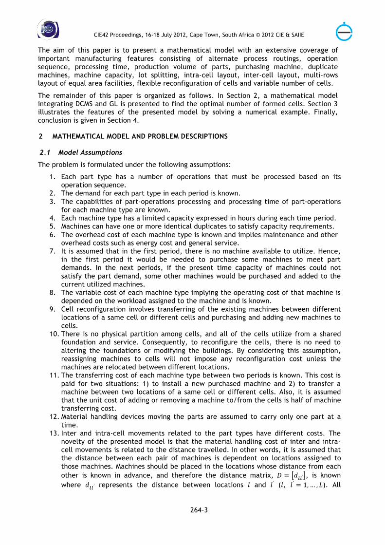
The objective function consists of seven cost components. Term (1.1) is the intra-cell material handling cost. Term (1.2) denotes the inter-cell material handling cost. Term (1.3) represents the cost of reconfiguration of cells. Term (1.4) is the purchase costs of new machines. Term (1.5) incorporates the overhead costs for all type machines utilized in the cells. Term (1.6) takes into account the operating cost of all machine types. Term (1.7) is the total cost of forming cells.

Inequality (2) guarantees that each operation of a part is processed on the machine which is capable to process that operation. Constraint (3) shows that demand of each part can be satisfied in period t through internal production. Equation (4) describes that the number of machine type m utilized in the period t is equal to number of utilized machines of the same type in the previous period plus the number of new machines of the same type purchased at the beginning of the current period. Inequality (5) necessitates that the number of machines of all types utilized in the cells is less than the number of available locations. The cell size is limited through Constraints (6) and (7), where the cell size lies within the user defined lower and upper bounds. The order of forming cells is determined by Constraint (8).

Constraint (9) is related to the machine capacity. Constraints (10) and (11) are material flow conservation equations. Constraint set (12) is to ensure that each location can receive one machine at most and only belong to one cell, simultaneously. Constraints (13)-(15) provide the logical binary and non-negativity integer necessities for the decision variables.

3 ILLUSTRATIVE NUMERICAL EXAMPLE

To validate the proposed model and illustrate its various features, a numerical examples is solved using GAMS 22.0 software (solver CPLEX) on an Intel® CoreTM2.66 GHz Personal


264-7

Computer with 4 GB RAM. The information related to this example is given in Tables 1 and 2. This example which is taken from the previous study by Kia et al., [4] consists of four part types, five machine types and two periods, in which each part type is assumed to have three sequential processing operations. Each operation can be processed on two alternative machines. Five columns of Table 1 contain the information related to the machine time capacity, relocation cost, purchasing machine cost, overhead cost, and machine operating cost. For more simplicity, the capacity of all machines is assumed to be equal to 500 hours per period. Furthermore, the processing time of each operation for all part types are presented in Table 1. The demand quantity for each part type and also the product mix for each period are presented in Table 1. Intra and inter-cell material handling costs per each part type are 5 and 50, respectively. Also, forming cell cost is considered as 20000 units per cell.

Table 1: Machine And Part Information

P4 P3 P2 P1 Machine info.

3 2 1 3 2 1 3 2 1 3 2 1 βm αm γm δm Tm

0.83 0.49 0.46 0.39 0.65 0.76 9 1800 18000 900 500 M1 0.74 0.33 0.99 0.79 7 1500 15000 750 500 M2

0.45 0.57 0.44 0.93 0.73 5 1800 18000 900 500 M3 0.14 0.80 0.46 9 1700 17000 850 500 M4

0.62 0.67 0.48 0.93 0.65 0.54 8 1300 13000 650 500 M5 0 300 700 200 Dpt 300 700 250 500

The maximum number of cells which are allowed to be formed in each period is 4. Also, the lower and upper sizes of cells are 2 and 3, respectively. The distances between eight locations existing in the shop floor are presented in the matrix, as shown in Table 2.

Table 2: Distance Matrix Between Locations

Locations L1 L2 L3 L4 L5 L6 L7 L8

L1 0 1 2 1 2 3 2 3

L2 1 0 1 2 1 2 3 2

L3 2 1 0 3 2 1 4 3

L4 1 2 3 0 1 2 1 2

L5 2 1 2 1 0 1 2 1

L6 3 2 1 2 1 0 3 2

L7 2 3 4 1 2 3 0 1

L8 3 2 3 2 1 2 1 0

The obtained solution with the developed model presented in this paper on the explained example is detailed out in the following. Also, to show the advantages of the proposed model considering variable number of cells in compare to previous model (Kia et al., [4]), the solutions obtained using two models and their performance are discussed in the rest.

The optimal solution is obtained after 74159 seconds (i.e., about 20 hours). Table 3 shows the part-operation allocations to all the machines located in locations of cells for two periods.


264-8

Period 1

Period 2

Table 3: Machine Locations And Part-Operation Allocations To The Machines

P4 P3 P2 P1 Machine info

3 2 1 3 2 1 3 2 1 3 2 1 L M C 484 1 M4 C1 199 484 4 M5 501 216 216 7 M1 160 2 M5 C2 300 300 5 M2 140 200 200 200 8 M3

P4 P3 P2 P1 Machine info 3 2 1 3 2 1 3 2 1 3 2 1 L M C

700 13 262 1 M4 C1 300 300 71 71 4 M5

300 166 166 237 7 M1 700 13 13 262 2 M5 C2 700 262 5 M2

238 238 238 8 M3

The cell configurations and machine layout for two periods corresponding to the best solutions obtained using model presented by Kia et al. [4] with three predetermined cells and the proposed model with two optimal cells are shown in Figure 1 and Figure 2, respectively. This figures show some of the characteristics and advantages of the proposed model with variable number cells. As can be seen, for the model with optimal number of cells, two cells in each period are formed that reduces the forming cell cost in compare to the previous model where forming three cells was predetermined by system designer. Also, in the first period one quantity of machine types 1, 2, 3 and 4 and two quantities of machine type 5, in total 6 machines, are purchased. In the second period, it is not required to purchase new machines and increase the available machine capacity. In the first period, machine types 4, 5 and 1 are assigned to cell 1 and located in locations 1, 4 and 7, respectively. Furthermore, in the first period machine types 5, 2 and 3 are assigned to cell 2 and located in locations 2, 5 and 8, respectively. In the second period, the locations of machines will be unchanged, however the configuration of cells will be changed as machine type 4 (M4) assigned to cell 1 and located in location 1 (L1) in period 1 would be assigned to cell 2 in period 2 and in a similar way machine M3 assigned to cell 2 and located in L8 in period 1 would be assigned to cell 1 in period 2. As a result, relocating machines is not necessary between two successive periods. Since there is no machine relocation between periods, the only cost which is incurred for relocation is related to installing new purchased machines in the first period.

Also, as a further illustration of the material flows between the machines, they are represented by directed arcs in Figure 2. For instance, in period 1 the quantity of the first operation of part 2 processed on machine 4 in location 1 of cell 1 is 484 units, from which 199 parts are processed by operations 2 and 3 on the machine 5 in location 4 of cell 1, and the remaining 285 units are processed by operation 3 on the machine 1 in location 7 of cell 1. By considering the material flows of part 1 in period 1, all operations of part 1 are processed on M3 in cell 2, so no inter or intra-cell material handling costs are incurred.

Comparing material flows between Figure 1 and Figure 2 illustrates that process plan for parts have been completely changed. This result shows that changing in the number of formed cells could dramatically influence on the processing plan of parts.


264-9

Figure 1: Best Obtained Cell Configurations, Machine Layout And Material Flow With

Predetermined Number Of Cells (Three Cells In Each Period).

Figure 2: Best Obtained Cell Configurations, Machine Layout And Material Flow With Optimal Number Of Cells (Two Cells In Each Period).

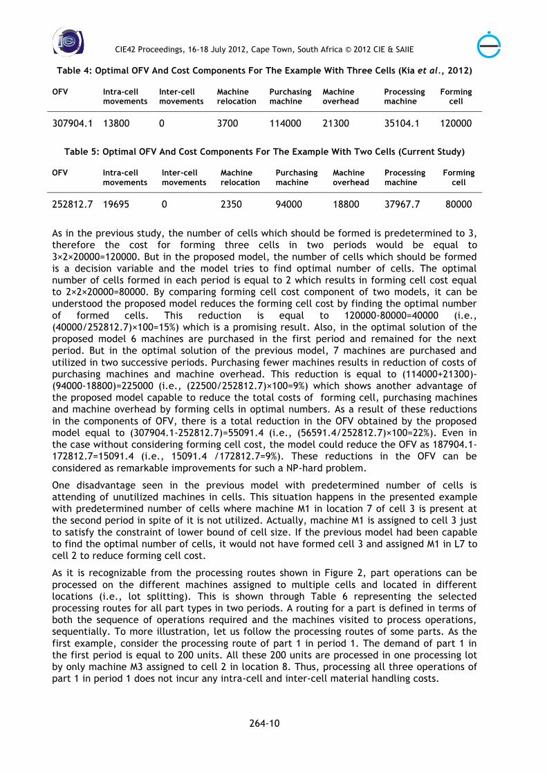
Here, the Objective Function Value (OFV) obtained in this paper is compared to the previous study by Kia et al. [4]. In order to compare two mathematical models, they should have same components. Therefore, the costs of forming cells should be added to OFV of the previous study. The optimal OFV and cost components for the example obtained by the previous study with three cells and proposed model with 2 cells (i.e., the optimal number of formed cells) are presented in Tables 4 and 5, respectively.


264-10

Table 4: Optimal OFV And Cost Components For The Example With Three Cells (Kia et al., 2012)

Forming cell

Processing machine

Machine overhead

Purchasing machine

Machine relocation

Inter-cell movements

Intra-cell movements

OFV

120000 35104.1 21300 114000 3700 0 13800 307904.1

Table 5: Optimal OFV And Cost Components For The Example With Two Cells (Current Study)

Forming cell

Processing machine

Machine overhead

Purchasing machine

Machine relocation

Inter-cell movements

Intra-cell movements

OFV

80000 37967.7 18800 94000 2350 0 19695 252812.7

As in the previous study, the number of cells which should be formed is predetermined to 3, therefore the cost for forming three cells in two periods would be equal to 3×2×20000=120000. But in the proposed model, the number of cells which should be formed is a decision variable and the model tries to find optimal number of cells. The optimal number of cells formed in each period is equal to 2 which results in forming cell cost equal to 2×2×20000=80000. By comparing forming cell cost component of two models, it can be understood the proposed model reduces the forming cell cost by finding the optimal number of formed cells. This reduction is equal to 120000-80000=40000 (i.e., (40000/252812.7)×100=15%) which is a promising result. Also, in the optimal solution of the proposed model 6 machines are purchased in the first period and remained for the next period. But in the optimal solution of the previous model, 7 machines are purchased and utilized in two successive periods. Purchasing fewer machines results in reduction of costs of purchasing machines and machine overhead. This reduction is equal to (114000+21300)-(94000-18800)=225000 (i.e., (22500/252812.7)×100=9%) which shows another advantage of the proposed model capable to reduce the total costs of forming cell, purchasing machines and machine overhead by forming cells in optimal numbers. As a result of these reductions in the components of OFV, there is a total reduction in the OFV obtained by the proposed model equal to (307904.1-252812.7)=55091.4 (i.e., (56591.4/252812.7)×100=22%). Even in the case without considering forming cell cost, the model could reduce the OFV as 187904.1-172812.7=15091.4 (i.e., 15091.4 /172812.7=9%). These reductions in the OFV can be considered as remarkable improvements for such a NP-hard problem.

One disadvantage seen in the previous model with predetermined number of cells is attending of unutilized machines in cells. This situation happens in the presented example with predetermined number of cells where machine M1 in location 7 of cell 3 is present at the second period in spite of it is not utilized. Actually, machine M1 is assigned to cell 3 just to satisfy the constraint of lower bound of cell size. If the previous model had been capable to find the optimal number of cells, it would not have formed cell 3 and assigned M1 in L7 to cell 2 to reduce forming cell cost.

As it is recognizable from the processing routes shown in Figure 2, part operations can be processed on the different machines assigned to multiple cells and located in different locations (i.e., lot splitting). This is shown through Table 6 representing the selected processing routes for all part types in two periods. A routing for a part is defined in terms of both the sequence of operations required and the machines visited to process operations, sequentially. To more illustration, let us follow the processing routes of some parts. As the first example, consider the processing route of part 1 in period 1. The demand of part 1 in the first period is equal to 200 units. All these 200 units are processed in one processing lot by only machine M3 assigned to cell 2 in location 8. Thus, processing all three operations of part 1 in period 1 does not incur any intra-cell and inter-cell material handling costs.


264-11

To say another example, consider the demand of part type 2 which is 250 units in the second period. Then, 250 units are split in three different processing lots.

Two of them are processed in a same cell (i.e., cell 1) and the third lot is processed in cell 2. Then a form of lot splitting is implemented by dividing the production lot between two cells 1 and 2.

Another form of lot splitting is for the second operation of part 2 in period 1 processed in C1 as 484 units are processed by the second operation on machine M5, located in L4, whilst 285 units are transferred to machine M1, located in L7 and the remaining 199 units are again processed on machine M5, located in L4 to complete production.

Table 6: Processing Routes For Parts In Two Periods

Period 1

Operations

Part No. 1 2 3 Part demand

1 200/M3/L8/C2 200/M3/L8/C2 200/M3/L8/C2 200

2 199/M4/L1/C1 199/M5/L4/C1 199/M5/L4/C1

700 285/M4/L1/C1 285/M5/L4/C1 285/M1/L7/C1

216/M1/L7/C1 216/M1/L7/C1 216/M1/L7/C1

3 160/M5/L2/C2 160/M2/L5/C2 160/M5/L2/C2 300 140/M3/L8/C2 140/M2/L5/C2 140/M3/L8/C2

4 0

Period 2

Operations

Part No.

1 2 3 Part demand

1 238/M3/L8/C1 238/M3/L8/C1 238/M3/L8/C1 500

262/M5/L2/C2 262/M2/L5/C2 262/M4/L1/C2

2 166/M1/L7/C1 166/M1/L7/C1 166/M1/L7/C1

71/M1/L7/C1 71/M5/L4/C1 71/M5/L4/C1 250

13/M4/L1/C2 13/M5/L2/C2 13/M5/L2/C2

3 700/M4/L1/C2 700/M5/L2/C2 700/M2/L5/C2 700

4 300/M1/L7/C1 300/M5/L4/C1 300/M5/L4/C1 300

4 CONCLUSION

In this paper, a mixed-integer non-linear programming model for the dynamic cellular manufacturing system (DCMS) design integrated with group layout and several manufacturing attributes was proposed. Our presented model was capable to determine the optimal cell configuration, machine locations, optimal number of cells to be formed and process plan for each part type at each period over the planning horizon.

The advantage of the proposed model in compare to previous study (Kia et al., [4]) is considering the number of formed cells as a decision variable. As it was shown in the presented example, finding the optimal number of cells which should be formed in each period enables the


264-12

proposed model to reduce costs up to 22% in a small-sized problem. It is obvious that in large-sized problems, predetermining the number of cells by system designer can even prevent the model to find optimal strategy in forming cells and reach minimum total costs.

The presented numerical example clarified that considering variable number of cells brings flexibility for the model to form cells more economically.

Comparing cell configurations in two periods obtained by the proposed model with two optimal cells and the previous study with 3 cells showed that the proposed model can handle varying demand by undergoing less cell reconfiguration. This is another advantage of the proposed model with variable number of cells.

5 REFERENCES

[1] Ahkioon, S. Bulgak, A.A. Bektas, T. 2009. Cellular manufacturing systems design with routing flexibility, machine procurement, production planning and dynamic system reconfiguration. Int. J. of Production Research, 47(6), pp 1573-‐1600.

[2] Defersha, F.M. Chen, M. 2006. A comprehensive mathematical model for the design of cellular manufacturing systems. Int. J. of Production Economics 103, pp 767–783.

[3] Jolai, F. Tavakkoli-Moghaddam, R. Golmohammadi, A. Javadi, B. 2011. An Electromagnetism-like algorithm for cell formation and layout problem. Expert Systems with Applications, doi:10.1016/j.eswa.2011.07.030.

[4] Kia, R. Baboli, A. Javadian, N. Tavakkoli-Moghaddam, R. Kazemi, M. Khorrami, J. 2012. Solving a group layout design model of a dynamic cellular manufacturing system with alternative process routings, lot splitting and flexible reconfiguration by simulated annealing. Computers & Operations Research, 39, pp 2642–2658.

[5] Mahdavi, I. Aalaei, A. Paydar, M.M. Solimanpur, M. 2010. Designing a mathematical model for dynamic cellular manufacturing systems considering production planning and worker assignment, Computers and Mathematics with Applications, doi:10.1016/j.camwa.2010.03.044.

[6] Rheault, M. Drolet, J. Abdulnour, G. 1995. Physically reconfigurable virtual cells: a dynamic model for a highly dynamic environment. Computers & Industrial Engineering, 29 (1–4), pp 221–225.

[7] Saidi-Mehrabad, M. Safaei, N. 2007. A new model of dynamic cell formation by a neural approach, Int. J. of Advanced Manufacturing Technology, 33, pp 1001–1009.

[8] Safaei, N. Saidi-Mehrabad, M. Jabal-Ameli, M.S. 2008. A hybrid simulated annealing for solving an extended model of dynamic cellular manufacturing system. Eur. J. of Operational Research, 185, pp 563–592.

[9] Solimanpur, M. Vrat, P. Shankar, R. 2004. Ant colony optimization algorithm to the inter-cell layout problem in cellular manufacturing. Eur. J. of Operational Research, 157, pp 592–606.

[10] Tavakkoli-Moghaddam, R. Javadian, N. Javadi, B. Safaei, N. 2007. Design of a facility layout problem in cellular manufacturing systems with stochastic demands. Applied Mathematics and Computation, 184, pp 721–728.

[11] Wu, X. Chu, C.H. Wang, Y. Yan, W. 2007. A genetic algorithm for cellular manufacturing design and layout. Eur. J. of Operational Research, 181, pp156–167.

[12] Wemmerlov, U. Hyer, N.L. 1986. Procedures for the part family/machine group identification problem in cellular manufacture. J. of Operations Management, 6, pp 125–147.

a mathematical model for designing group layout of …

Documents