ESTIMATING UNITED STATES PHILLIPS CURVES WITH EXPECTATIONS

CONSISTENT WITH THE STATISTICAL PROCESS OF INFLATION*

Bill Russell

1 November 2011

ABSTRACT

‘Modern’ theories of the Phillips curve predict inflation is an integrated, or

near integrated, process. However, inflation appears bounded above and

below in developed economies and so cannot be ‘truly’ integrated and more

likely stationary around a shifting mean. If agents believe inflation is

integrated as in the ‘modern’ theories then they are making systematic errors

concerning the statistical process of inflation. An alternative theory of the

Phillips curve is developed that is consistent with the ‘true’ statistical process

of inflation. It is demonstrated that United States inflation data is consistent

with the alternative theory but not with the ‘modern’ theories of the Phillips

curve.

Keywords: Phillips curve, inflation, structural breaks, GARCH, non-

stationary data

JEL Classification: C22, C23, E31

Presented on 2 November 2011 at the Department of Economics Seminar Series,

Birmingham Business School, University of Birmingham.

* Bill Russell, Economic Studies, School of Business, University of Dundee, Dundee DD1 4HN, United

Kingdom. +44 1382 385165 (work phone), +44 1382 384691 (fax), email brussell@brolga.net. I would like

to thank Arnab Bhattacharjee, Hassan Molana, Denise Petrie and Genaro Sucarrat for their helpful

comments and advice. All data are available at http://billrussell.info.

2

1. INTRODUCTION

A notable shortcoming of the Friedman-Phelps (F-P) expectations augmented, New

Keynesian (NK) and hybrid theories of the ‘modern’ Phillips curve is that they predict

inflation is an integrated, or very near integrated, statistical process and that this prediction is

a direct result of the personal characteristics of the agents in all three models.1 For example,

in the F-P model this prediction is due to the assumption that agents hold adaptive

expectations. In the NK model the coefficient on expected inflation is equal to the discount

rate of households and firms. The idea the statistical process of inflation is due to a

characteristic of agents and not due to the behaviour of central banks in response to shocks to

inflation is an anathema to standard monetary theory where central banks set monetary policy

which in turn determines the long-run rate of inflation. Furthermore, as inflation in developed

economies appears to have an upper boundary at some moderate rate and a lower boundary

around zero it is unlikely inflation can be ‘truly’ integrated.

While inflation appears not to be an integrated process it is likely that inflation is non-

stationary.2 For example, to argue the converse that inflation is stationary implies, (i) the

stance of monetary policy is unchanging leading to a constant mean rate of inflation, (ii) there

is only one expected rate and associated long-run rate of inflation implying there is only one

short-run Phillips curve, and (iii) the original Phillips (1958) curve of did not ‘break-down’

with changes in the expected rate of inflation towards the end of the 1960s. Furthermore, a

constant mean rate of inflation implies that all the ‘modern’ theories of the Phillips curve

since Friedman (1968) and Phelps (1967) are irrelevant on an empirical level as there has

been no change in the expected rate of inflation. Unless we are comfortable with the

implications of inflation as a stationary process we need to conclude that inflation is a

stationary process around shifting means. This would allow for the numerous long-run and

expected rates of inflation which are a central component of modern theories of the Phillips

1 The F-P and hybrid theories predict that the sum of the dynamic inflation terms sum to one. In the NK

model the coefficient on expected inflation is the discount rate which for a risk neutral agent, quarterly data

and a real rate of inflation of four per cent is around 0.99. However, the empirical NK literature largely

ignores this and considers the sum of the dynamic inflation terms to be one. For simplicity of exposition we

will assume the sum of the coefficients on the dynamic inflation terms in the NK and hybrid models is one

unless otherwise stated.

2 The term non-stationary in this paper encompasses all statistical processes other than stationary with a

constant mean. It therefore includes stationary around a shifting mean.

3

curve. Furthermore, deviations from any particular mean rate of inflation are partly due to

exogenous shocks to inflation and partly due to the response of monetary policy to those

shocks.3

One might also question the role that agents play in the modern theories of the Phillips curve.

The agents that populate these theories are very sophisticated and very well informed so as to

undertake the proposed highly sophisticated optimising behaviour in these models. Therefore

it is inconsistent with the sophisticated nature of the agents that they do not understand

something as simple as the ‘true’ statistical process of inflation. In particular, a sophisticated

agent is unlikely to make the systematic error over fifty or more years of believing that

inflation has a constant mean or is an integrated process. Consequently, an attractive

characteristic of any model of how agents form inflation expectations would be that agents do

not make systematic errors concerning the ‘true’ statistical process of inflation. In particular,

the information set of rational agents should include an understanding of the ‘true’ statistical

process of inflation and that this set cannot include the mistaken belief that inflation is (i)

integrated or (ii) stationary with a constant mean. We therefore propose a model of

expectation formation which is consistent with the statistical process of inflation.

The empirical Phillips curve literature also has its shortcomings. First, the literature that

seeks to validate the competing modern theories fails to model the heteroscedastic nature of

inflation over the past five decades. Graph 1 of United States quarterly inflation for the

period March 1960 to December 2010 shows the variance in inflation increasing during the

turbulent high inflation years of the 1970s before declining to lower levels following the

‘Volker deflation’ in the early 1980s.4 This ‘clustering’ of high and low variance into discrete

periods suggests that the variance in inflation may be serially correlated.5 Since Engle (1982,

1983), a popular way to accommodate both these characteristics of inflation data is to estimate

one of a wide range of auto-regressive conditional heteroscedastic (ARCH) type models of

3 Russell (2006, 2011) makes this argument concerning the ‘true’ statistical process of inflation in more

detail.

4 Inflation is measured in Graph 1 as the quarterly change in the natural logarithm of the gross domestic

product (GDP) implicit price deflator at factor cost multiplied by 400 to provide an ‘annualised’ rate of

inflation. See the Data Appendix for details of the data used in this paper.

5 This suggestion is borne out by an ARCH LM test of the residuals from an AR(4) model of United States

inflation which rejects the null hypothesis of homoscedastic errors with a probability of 0.0101.

4

inflation.6 Much of the ARCH literature on inflation has focused on (i) the unpredictability of

inflation when the variance increases; and (ii) the relationship between the mean and the

variance of inflation.7 Interest in the former is due to the welfare costs associated with agents

holding mistaken inflation expectations and the later due to Friedman’s (1977) conjecture in

his Nobel Prize lecture that the mean rate of inflation and the variance of inflation are

positively related.

This brings us to the second shortcoming of the empirical Phillips curve literature where most

work proceeds under the assumption that inflation is either stationary or integrated. These

assumptions are difficult to sustain as argued above. If instead we consider inflation to be a

stationary process around a shifting mean then not accounting for the breaks may be the

source of the observed heteroscedasticity in the inflation data. Consequently, if the shifts in

mean are accounted for in the estimation process then the conditional variance may be

constant and the data homoscedastic. We would then conclude that the observed

heteroscedastic nature of inflation has no economic or behavioural relevance and simply

reflects the unaccounted breaks in the mean rate of inflation in the empirical analysis. A

further shortcoming of the empirical Phillips curve literature is that assuming inflation is

either stationary or integrated will lead to biased estimates of Phillips curves.8 Russell (2011)

and Russell, Banerjee, Malki and Ponomareva (2011) demonstrate using United States data

that not adequately accounting for the shifts in mean inflation lead to severely biased

estimates.

The shifting mean rate of inflation is also evident in Graph 1. These shifts can be identified

formally by applying the Bai and Perron (1998, 2003a, 2003b) technique to identify multiple

breaks in the mean rate of inflation.9 Nine breaks in mean are identified in the inflation data

implying there are ten inflation ‘regimes’ within which we believe statistically the mean rate

6 In his seminal Nobel Prize winning paper Engle (1982) introduces the ARCH methodology and

demonstrates the technique on a model of United Kingdom inflation. There is a wide range of excellent

survey articles on the ARCH methodology including those of Bollerslev, Chou and Kroner (1992),

Bollerslev, Engle and Nelson (1994) and Engle, Focardi and Fabozzi (2008).

7 For example, see Engle (1982, 1983, 1988), Cosimano and Jansen (1988), Baillie, Chung and Tieslau

(1996), Grier and Perry (2000) and Boero, Smoth and Wallis (2008).

8 This is a generalisation of the Perron (1989, 1990) argument that stationary processes with breaks are easily

mistaken for integrated processes.

9 See Appendix 2 for details of the Bai-Perron estimated breaks in the mean rate of inflation.

5

of inflation is constant. The identified mean rates of inflation in each regime are shown on

Graph 1 as solid thin horizontal lines. On a visual level the technique appears to have

identified all the major shifts in mean over the past fifty years.

This paper therefore considers two questions. First, do Phillips curve that models inflation

expectations in a way that is consistent with the statistical process of inflation dominate the

existing three ‘modern’ theories of the Phillips curve? And second, are estimates of the

‘modern’ Phillips curves affected in any meaningful way by accounting for the

heteroscedastic nature of inflation?

In the next section we begin by briefly setting out the modern theories of the Phillips curve so

as to identify the source of the prediction that inflation is an integrated, or near integrated,

process. Section 3 suggests a ‘fourth way’ to estimating Phillips curves where the formation

of expectations is consistent with agents knowing the statistical process of inflation. Section 4

sets out and Section 5 estimates a general hybrid model of inflation that nests all four theories

of the Phillips curve and allows for possible ARCH effects and shifting means in the data.

This model simultaneously estimates ten short-run Phillips curves for the United States

associated with the ten identified mean, or long-run, rates of inflation shown in Graph 1. We

find that once we account for the shifts in the mean rate of inflation, there is no evidence that

expected inflation as commonly measured in the New Keynesian literature plays a significant

role in the dynamics of inflation. We also find that the data is inconsistent with the standard

interpretations of both the Friedman-Phelps and hybrid models of the data. In contrast, we

find evidence that the alternative Phillips curve proposed in Section 3 that incorporates

expectations based on knowledge of the statistical process of inflation is consistent with the

data.

2. ‘MODERN’ THEORIES OF THE PHILLIPS CURVE

The ‘modern’ theories of the Phillips curve are all ‘expectation’ based and incorporate an

inflation equation:

tzttt zE 1 (1)

6

where the rate of inflation, , in period t depends on expected inflation, 1ttE ,

conditioned on information available in period t and a ‘forcing’ variable, tz . The latter is

measured in a number of ways in the literature including the unemployment rate, the gap

between the unemployment rate and some measure of its long-run value, the gap between

output and its potential level, real marginal costs, labour’s income share and the markup of

prices over unit labour costs. Since Friedman (1968) and Phelps (1967), all three theories

believe on an empirical level at least that the ‘correct’ long-run value of is one so that the

long-run Phillips curve is ‘vertical’. Leaving aside the different forcing variables, what

differentiates these models of inflation is how expected inflation is dealt with in the inflation

equation. We now briefly describe the F-P, NK and hybrid theories so as to identify what

determines the size of in equation (1) in each model.

2.1 The Friedman-Phelps Phillips Curve

The expectations augmented Phillips curve of Friedman (1968) and Phelps (1967) assumes

adaptive expectations of the form:

1111 ttttttt EEE (2)

where errors in the expectation of inflation are partially eradicated in each period.

Cagan (1956) is the first to incorporate adaptive expectations into estimated models of

inflation and refers to as the ‘coefficient of expectations’ which represents how quickly

expected rates of inflation adjust to actual rates of inflation. Backward induction of adaptive

expectations implies that expected inflation is a geometrically declining distributed lag of all

past rates of inflation such that:

it

i

i

ttE

1

1 (3)

where 110

i

i . Substituting equation (3) into (1) provides;

tzit

i

i

t z

1

1 (4)

7

On a practical level equation (4) cannot be estimated with an infinite number of lags. Using

the Kyock (1954) transformation we can truncate the number of lags and re-write (4) as:10

tzttzttt zz 1111 (5)

which can be thought of as the F-P Phillips curve. Other possible transformations include that

of Almon (1965) and the ‘rational distributed lag function’ of Lucas and Rapping (1969).

However that to conform with the F-P Phillips curve the lagged inflation terms must sum to

one over the truncated number of lags so that there is no long-run trade-off between the

nominal variable, t , and the real variable, tz .

Note three aspects of equation (5). One, the predication that the sum of the dynamic terms

equals 1 is a direct result of the assumption of adaptive expectations and not due to any

underlying optimising behaviour of the agents in the model. Two, the desire for the dynamic

inflation terms to sum to one is so that long-run money neutrality is maintained in the model.

And three, adaptive expectations have a long acknowledged (at least in the rational

expectations literature) unappealing implication that agents make systematic errors while they

are converging on the long-run rate of inflation.

2.2 The New Keynesian Phillips Curve

The N-K Phillips curve responds to two perceived short-comings of the F-P Phillips curve by

providing optimising microeconomic foundations for the Phillips curve and agents no longer

make systematic errors in their expectations through the use of rational expectations. While

there are numerous versions of the NK model, for our purpose the basic NK model of Gali

(2008) provides a very clear general exposition of NK Phillips curve.11

10 Nerlove (1956) combines the adaptive expectations of Cagan (1956) and the Koyck (1954) transformation

to provide the result shown in equation (5). For a clear survey of the econometrics of early distributed

lagged models see Griliches (1967).

11 Gali (2008) sets out a very clear and well-argued basic NK model. The nomenclature used here is the same

as that used by Gali where further details and extensions of the model can be found. Note that for our

purposes using Gali’s basic model as a ‘representative’ NK model introduces no loss due to generality as we

only wish to identify what determines in equation (1). Alternatively a clear exposition can also be found

in Woodford (2003).

8

Gali’s basic NK model comprises households and firms. Households undertake inter-

temporal optimisation and are price takers in both goods and labour markets. In keeping with

a standard classical macroeconomic model, firms also optimise but in contrast with the

classical model firms set prices for a differentiated product and follow Calvo (1983) price

setting.

In the basic NK model there is a representative infinitely-lived household that seeks to

maximise its objective function:

0

0 ,t

tt

t NCUE (6)

where tC is a consumption index and tN is the hours of employment. The utility function,

U , is continuous and twice differentiable, and t is the discount rate in period t that

households apply to future consumption and employment. Assuming there is a continuum of

goods represented by the interval [0, 1] the household budget constraint in period t can be

represented as:

1

0

1 tttttttt TNWBBQdiiCiP (7)

where iPt is the price of the differentiated goods represented by the interval [0, 1], tW is the

nominal wage rate, tB is the quantity of riskless discount bonds that are purchased in period t

and mature in 1t with price tQ , and tT are lump sum taxes net of lump sum non-labour

income. The decision for households is somewhat complicated because they have to

simultaneously optimise their consumption, tC , over time and over the range of differentiated

goods within each period.

Gali demonstrates that the log-linear optimal consumption and labour decisions from this

model can be approximately described by:

tttt ncpw (8)

9

11

1tttttt EicEc (9)

where lower case variables are in natural logarithms, log is the discount rate and

tQi log is the riskless nominal interest rate.

Firms in the NK model are assumed to lie on a continuum indexed 1,0i and produce

differentiated goods, )(iY , using identical technology, tA , and with a production function:

1iNAiY ttt (10)

Following Calvo (1983), individual firms reset prices optimally in each period with

probability which is independent of the time that has elapsed since the firm last

changed prices and that as is the probability that firms do not adjust prices it can therefore

be considered as one of many indexes of price stickiness.

From these basic building blocks, Gali shows an approximate log-linear form of the dynamics

of aggregate prices can be described as:

11

ttt pp (11)

where

tp is the optimal price set by firms that reset prices in period t . Equation (11)

suggests that inflation in period t in the NK model is due to the deviation between the

aggregate price index and the optimal price. Note that the aggregate price index is itself a

weighted average of optimal and suboptimal non-reset prices.

The optimal price can then be shown to be:

0

|1k

kttktt

k

t pmcEp (12)

where is the log of the desired markup, is the discount factor for the firms nominal

future returns and equal to the discount rate of households, and is the real marginal costs

10

of production. Equation (12) suggests that the firm when optimally adjusting prices will

choose a desired markup, , over a weighted average of marginal costs in the current and

future periods where the weights are the probabilities that the price is unchanged over each

horizon, k .

Finally, Gali demonstrates that the NK inflation equation is:

tttt E ˆˆˆ1 (13)

where indicates the deviation from the steady state values of inflation and the markup,

1

111 and the model is solved around a zero steady state rate of

inflation. Equation (13) is the NK Phillips curve in inflation-markup space but equivalent NK

Phillips curves can be derived in inflation-output gap and inflation-unemployment rate gap

space. Consequently, the defining feature of the NK model is that current inflation depends

on the discounted value of expected inflation.

Solving forward equation (13) provides:

0

ˆˆk

tt

k

t E (14)

which reveals the role that the markup plays in inflation dynamics in this NK model. When

the markup is below its steady state value, firms that reset their prices will choose an optimum

price above the aggregate price level leading to high inflation and vice versa.

Finally, for our purposes there are three aspects to this basic NK Phillips curve to be noted.

One, the basic NK curve is solved around the steady state of zero inflation and does not

explicitly explain how inflation adjusts to changes in steady state rates of inflation. Two,

is the discount rate and therefore a parameter inherent to the personal characteristics of the

agents in households and firms. And three, the discount rate is slightly less than 1. If

households and firms are risk neutral, face a symmetrical loss function in the region of the

optimum price, p , and their expectations about future prices are unbiased then assuming a

real interest rate of four per cent per annum the quarterly value of is in the order of 0.99.

11

However, there is considerable evidence that households and firms are risk averse.

Furthermore, the loss function around the optimum price that firms and households face may

be very asymmetrical. Firms risk closure by setting too high a price but only higher sales and

slightly lower profits if the price is set too low. Similarly, households that fund high levels of

current consumption as a result of mistaken price expectations risk bankruptcy while sub-

optimal consumption plans may only marginally lower utility. In these cases the gross

discount rate that incorporates a risk premium may be larger than in the basic NK model and

it is not difficult to imagine the case where may be close, or equal, to zero. Furthermore,

the NK model leads to the following paradoxical result. Suppose monetary policy is

successful in targeting a low stable rate of inflation leading to inflation being stationary with a

constant mean then uncertainty about changes in the mean rate of inflation would decline.

This would cause the risk premium to decline and the gross value of would increase along

with inflation persistence. This suggests that successful monetary policy that leads to low

stable inflation causes inflation to become more and not less persistent which is the opposite

of what we might presumably expect.

2.3 The Hybrid Phillips Curve

One of the drawbacks to the NK model noted early on by Fuhrer and Moore (1995), Roberts

(1997) and Gali and Gertler (1999) among others is that it implies that reducing inflation is

costless if agents are rational and forward looking and that this appears inconsistent with the

general observation that anti-inflation policies are associated with large costs to aggregate

output. It was also noticed that contrary to the predictions of the NK Phillips curve, lagged

inflation plays a significant role in the dynamics of United States inflation. These empirical

observations led to the hybrid Phillips curve:

ttttt E ˆ1 11 10 (15)

which is a convex combination of the NK and F-P Phillips curves.12

Note two aspects of the

hybrid Phillips curve. One, the curve does not have explicit optimising micro-foundations.

12 Henry and Pagan (2004) provide a general overview of the hybrid model. Roberts (1997) argues the

formation of expectations is partly rational and partly adaptive. The lagged inflation term in the hybrid

12

And two, in as much as 1 the dynamic inflation terms sum to one is imposed with no

reference to any theory. Instead this constraint is based on prior beliefs handed down from

the original F-P and NK theories that the ‘true’ value for in equation (1) is one so that the

long-run Phillips curve is vertical.

3. EXPECTATIONS CONSISTENT WITH THE STATISTICAL PROCESS OF INFLATION

The F-P, NK and hybrid theories outlined above have three properties in common. One, in

equation (1) is predicted to be, or very nearly, one. Two, the sum of the coefficients on the

dynamic inflation terms is due to fundamental personal characteristics of the agents. Three,

these theories predict inflation is always an integrated, or very nearly an integrated, process

irrespective of the behaviour of central banks. To paraphrase Milton Friedman’s famous

quotation, inflation is always and everywhere an integrated phenomenon.13

This absolutely

contradicts the concept that the behaviour of the monetary authorities determines the mean

and the statistical process of inflation. It is also inconsistent with the bounded nature of

inflation which implies it cannot be an integrated process.

These models also imply that agents on a very fundamental level make systematic errors by

believing that the set of all possible statistical processes for inflation is a singleton set

containing only one element which is inflation is an integrated process. Consider the

expectations operator in equation (1) based on information available in period t . Given the

agents in these theories are extremely sophisticated and rich in information so as to undertake

the necessary optimising behaviour contained within the models, these same agents for fifty

or more years fail to notice that inflation is a bounded variable and therefore not an integrated

process.14

We therefore hypothesise that the information set in period t should include

model can therefore be interpreted as due to a subset of agents who use adaptive expectations when setting

prices.

13 Milton Friedman’s original quotation is made in his Wincott Memorial Lecture delivered in London on 16

September 1970.

14 It is ironic that the very great majority of work estimating Phillips curves since Friedman (1968) and Phelps

(1967) make use of estimators that are unbiased only if inflation is a stationary process with a constant

mean which is in direct conflict with the important prediction of these models that the data should be

integrated. More recently when the data is treated as integrated the researchers fail to notice that the

inflation is bounded and so unlikely to be ‘truly’ integrated.

13

knowledge of key aspects of the statistical process of inflation and that the expectations

operator should be consistent with that knowledge.

Assume now that inflation is a stationary process around shifting means. In this case inflation

can be thought of as made up of two components. The first is the mean rate of inflation which

we model as subject to discrete shifts in monetary policy and highly persistent. The second is

the deviation of inflation from its mean value which may or may not be highly persistent.

Inflation in period t can therefore be written:

nn

tt (16)

where n is the mean rate of inflation in regime n . Furthermore, if the inflation equation (1)

is a valid description of the dynamics of inflation then the expectations operator in equation

(1) can be written:

nn

tttt fEE (17)

where ( ) is the mean reversion process. Valid functional forms for f depend in part

on what we assume agents ‘know’ at time t. We assume that agents know (i) that inflation is

a stationary process around shifting means and that shocks to inflation are mean zero and

stationary; and (ii) that other agents are not identical to themselves. This implies that agents

recognise that the observed mean revision process of inflation is an aggregation of the

disparate adjustment processes of non-identical agents. And consequently, the best an agent

can hope for if we eschew the unrealistic assumption of full information is to understand the

average adjustment process of all agents in the economy. Furthermore, without full

information agents can only infer the characteristics of the statistical process of inflation from

the published aggregate inflation data and not from a detailed understanding of all the non-

identical agents in the economy.15

15 In the modern theories of the Phillips curve the issue of how agents obtain the information concerning

future inflation is not discussed. Because these theories focus on individual agents and firms who are

identical it is implied that their expectations are based on their own experiences. However, in the ‘real

world’ it is not that straight-forward. If there are no changes in relative prices between the different forms

14

The idea that agents only understand the average mean reversion process of inflation is

helpful as it suggests that we only need to be able to approximate that process. Therefore, for

simplicity of exposition, we assume that inflation in continuous time follows an arithmetic

Poisson-Gaussian mean reversion process with shifts in mean of the form:

( ) (18)

where is from a standard normal distribution, is the long-run mean rate of inflation and

is the speed of adjustment back to the mean rate of inflation, is the volatility of inflation

and

is a Wiener increment and is the standard normal distribution. The shifts

in mean are introduced into the inflation process described by equation (18) by the counting

Poisson process :

{

( ) (19)

where is the probability distribution of the size of the mean shifts reflecting the arrival of

infrequent ‘news’ concerning shifts in the mean rate of inflation.

The mean shift distribution, , is difficult to estimate as the shifts in mean are ‘rare’ events

and so there is a lack of data. In our case there appears to be nine shifts in mean over a period

of fifty years. One practical approach is to assume the mean reversion process is independent

of the shifts in mean. This implies that the Wiener process, , driving inflation back to its

mean is uncorrelated with the Poisson process, , in equation (18) that drives the shifts in

mean. On a practical level we can then estimate the mean reversion process on its own and

of output in the long run then the mean rate of inflation of each form of output will be the same in the long

run although there may be some variation in the inflation rates of each firms output in the short run. But

what we know is that over the past five decades there have been large changes in relative prices due to

shifting demand, new products and different growth rates of productivity in different industries and firms.

Consequently, the experience of each firm in terms of their output price inflation over the past fifty years is

different and also different from aggregate price inflation. Consequently, while the firms output price

inflation is a predictor of aggregate inflation it is not necessarily a good predictor and is likely to be biased.

This suggests that firms may not be all that interested adjusting prices in line with aggregate inflation and

more likely to adjust prices in response to cost and demand conditions.

15

equation (18) collapses to an arithmetic Uhlenbeck and Ornstein (1930) process also known

as the Dixit and Pindyck (1994) model:16

( ) (20)

Finally, Dixit and Pindyck (1994) demonstrate that a first order autoregressive process in

discrete time is an approximation of the continuous time arithmetic U-O model of equation

(20):

(21)

where , the mean rate of inflation

, the adjustment process

( ), and the variance √ ( )

( ) where is the standard error from

estimating equation (21).

The appropriateness of estimating the mean reversion process independently of the process

driving the shifts in mean rests on the validity of assuming the two processes are uncorrelated.

Consider the nature of a mean shift and the information contained in lagged values of

inflation. Begin by assuming that a regime of n periods has a constant mean rate of inflation.

If agents can forecast the shift in mean j periods before the end of the regime then inflation in

the last j periods of the regime will begin to adjust to its new mean and therefore have a

different mean to the first n-j periods of the same regime. This contradicts the initial

assumption that the inflation regime has a constant mean.17

Therefore, during an inflation

regime where inflation has a constant mean it is not possible to forecast the impending shift in

mean and the assumption that the two processes are uncorrelated is valid along with

estimating the mean reversion process on its own. This conclusion conforms to our

understanding of structural breaks that they cannot, or at the very least, are very difficult to

forecast by the available information prior to the break.

16 See also Metcalf and Hasset (1995) and Epstein, Mayor, Schonbucher, Whalley and Wilmont (1998) for

practical applications of equation (20).

17 It may be that the transition between two stable regimes is made up of many small shifts in mean which we

cannot identify empirically with available techniques. However, the logic remains that each small shift is

not able to be forecasted from information contained in the existing regime.

16

Finally, substituting for ( ) in equation (17) and for { } in equation (1) provides an

expectation based Phillips curve consistent with the statistical process of inflation:

tz

n

ntt z 1 (21)

where expected inflation in period t is now correctly believed by agents to follow a mean

reverting process around a shifting mean and assuming random serially uncorrelated mean

zero shocks to inflation the criticism that the F-P model implies persistent unidirectional

deviations of expected inflation from its mean are not observed in equation (21).

4. A STRUCTURAL BREAK GARCH HYBRID PHILLIPS CURVE

To examine the empirical validity of the four Phillips curve theories outlined above we

estimate a 2SLS GARCH(q, p) hybrid Phillips curve allowing for structural breaks of the

form:

( ) ∑ (22)

where in the ‘mean’ equation (22) inflation, t , depends on expected inflation, 1ttE ,

conditioned on information available at time t , lagged inflation, 1t , a ‘forcing’ variable of

the markup, t , shift dummies representing the inflation ‘regimes’, , and an error term,

, due to the random errors of agents and the shocks to inflation. The conditional ‘variance’

equation is specified as a GARCH(q, p) process:

∑

∑

(23)

where the conditional variance, , is a linear function of a constant, , past forecast

variances (the GARCH term, ) and past squared residuals from the mean equation (the

ARCH term, ).

18 The ‘mean’ equation can be estimated asymptotically consistently with

18 The conditional variance is the one-period ahead forecasted variance conditioned, or based, on past

information. The GARCH model was introduced simultaneously by Bollerslev (1986) and Taylor (1986).

Note that Engle’s (1982) ARCH model is a special case of the GARCH model where .

17

two stage least squares (2SLS) but it will not be an efficient estimator when and

and the heteroscedasticity in the model is not accounted for.

The three ‘modern’ theories of the Phillips curve are nested within equation (22) and can be

thought of in terms of restrictions to equations (22) and (23). In the Friedman (1968) and

Phelps (1967) model 0f and 1b and agents are purely backward looking. At the

other extreme, the New Keynesian (NK) Phillips Curve models of Clarida, Galí and Gertler

(1999) and Svensson (2000) imply agents are purely forward-looking and df 1 and

0b where d is the discount rate. Finally, in the hybrid models of Galí and Gertler (1999)

and Galí, Gertler and Lopez-Salido (2001) agents are both backward and forward looking and

dbf 1 .

Our fourth ‘modern’ Phillips curve theory set out in Section 3 is also nested within the mean

equation (22). If 0f , 10 b and then the inflation data conforms with the

Phillips curve where expectations are consistent with the statistical process of inflation and

inconsistent with the F-P, NK and hybrid theories of inflation.

4.1 The Data

The model is estimated with quarterly seasonally adjusted United States data for the period

March 1960 to December 2010. Inflation is measured as the quarterly change in the natural

logarithm of the gross domestic product (GDP) implicit price deflator at factor cost. In

keeping with the recent NK and hybrid literatures the forcing variable is measured as the

natural logarithm of the price series divided by unit labour costs which is equivalent to the

inverse of labour’s income share. The shifts in the mean rate of inflation are identified in a

‘breaks in mean’ model of inflation:

t

k

i

iit D

1

1

(24)

The breaks in mean model is used instead of a breaks in an AR model of inflation as the bias

in the later coefficients is substantial due to the frequency and size of the breaks.

Consequently, with the later it is changes in the bias that may be identified as breaks. If the

18

bias is stable because the breaks in mean are frequent, large and evenly spaced then no break

will be identified even though the mean repeatedly shifts. Consequently, the only breaks that

will be identified is when there is a change in the bias such as between the 1970s and 1980s

when the structure and size of the breaks changes.

4.2 Expected Inflation and the Markup

Expected inflation, 1ttE , is measured as the forecasted value of inflation based on

information available at time t. It is measured by regressing inflation on lags of inflation and

the markup for periods t-2 to t-5. For models that include the regime dummies these are also

included in the regression. The regression is estimated using ordinary least squares and the

static forecast is included the estimation of the model with a lead of one period. Similarly, to

overcome simultaneity bias we replace the contemporaneous markup term with its static

forecast from regressing the markup on lags t-1 to t-4 of inflation and the markup as well as

the shift dummies in models where they are included. This means that the ordinary least

squares estimates of equation (22) are equivalent to 2SLS estimates of the same equation.

5. ESTIMATING UNITED STATES SHORT-RUN PHILLIPS CURVES

5.1 The Short-run Phillips Curve

So as to retrieve the standard results in the literature we begin by estimating the mean

equation (22) restricting the parameters on the regime shift dummies and ARCH terms to be

zero. Columns 1 and 2 in Table 1 report the hybrid and F-P models respectively which we see

are in general consistent with the standard Phillips curve literature. In column 1 we see that

without the breaks in mean and the ARCH effects (as in the standard literature) the sum of the

dynamic inflation terms are insignificantly different from 1 and the expected inflation term is

larger than lagged inflation which is interpreted as forward looking agents dominating

backward looking agents in the setting of prices. Note however that the forcing variable is

insignificant and that the models suffer from some serial correlation and considerable

heteroskedasticity. Similarly when we restrict the lead in inflation to zero the estimates

reported in column 2 are consistent with the F-P model with the estimated coefficient on

lagged inflation large (0.8079) but significantly less than 1. Again the model suffers from

considerable heteroskedasticity.

19

Columns 3 and 4 of Table 1 report the GARCH standard hybrid and F-P Phillips curves

without the inclusion of shift dummies. We find that the ARCH components are strongly

significant as in the standard ARCH inflation literature. Without accounting for the shifts in

mean the ARCH methodology appears to be statistically valid however the estimates of the

hybrid Phillips curve are not materially affected.19

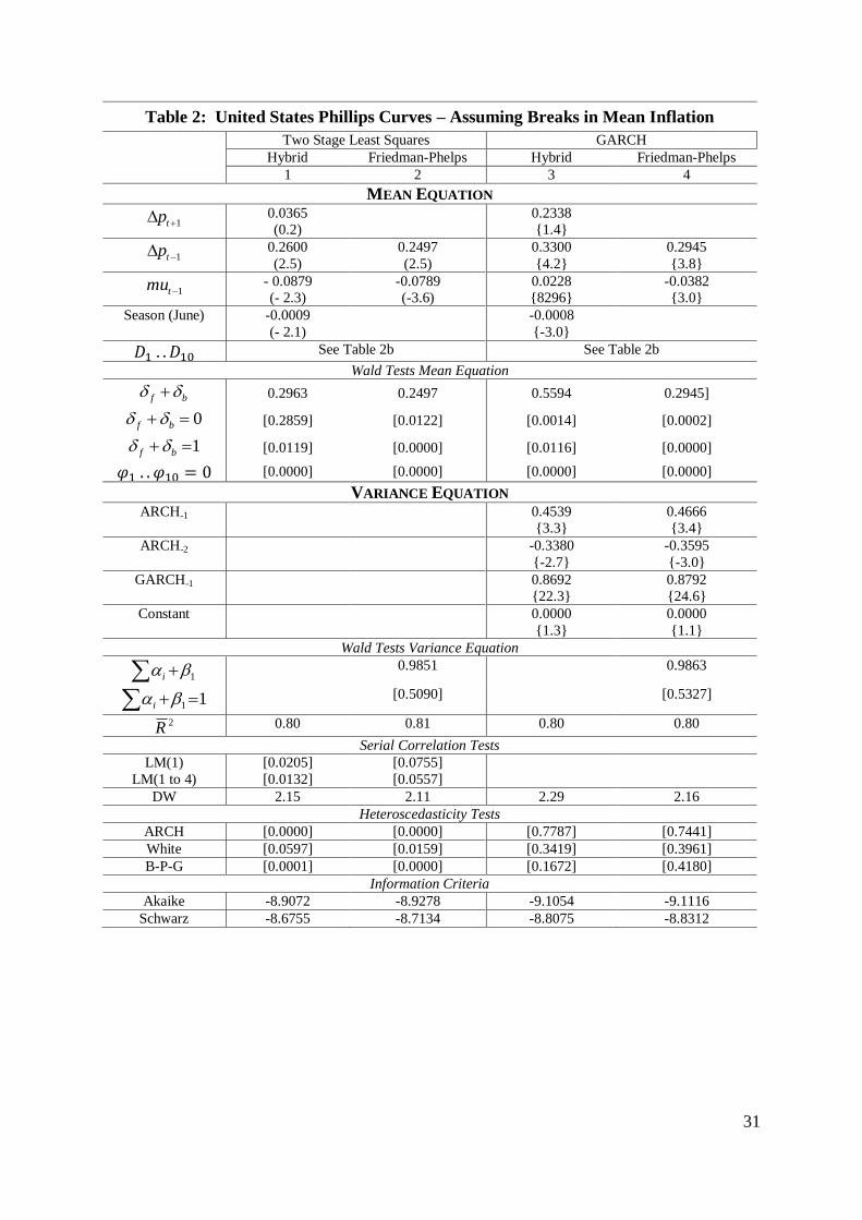
Turning now to the breaks in mean. Table 2 re-estimates the models incorporating the shift

dummies that represent the ten identified inflation regimes. In column 1 we find that

accounting for the shifts in mean the lead in inflation is now insignificant. Furthermore, in

the F-P model that excludes the lead in inflation the lag in inflation is significantly less than

one by a wide margin. Note also that both estimated models continue to suffer from

heteroskedasticity.

Finally, in columns 3 and 4 we report the estimates of our full GARCH models with structural

breaks. We see that the general estimates of the mean model are largely unaffected but the

ARCH and GARCH terms are highly significant. Note that with the expected inflation term

excluded the single lag in inflation is significant with an estimated value of 0.2945 which is

significantly less than one by a wide margin. The final model strongly rejects the restrictions

of the F-P, NK and hybrid models and strongly accepts the restrictions consistent with the

fourth ‘modern’ Phillips curve suggested above.

5.2 The Long-run Phillips Curve

In section 5.1 we estimate ten short-run Phillips curves for the ten mean, or long-run, rates of

inflation in the data. Given the data is stationary after the inclusion of the dummies it is not

surprising that the sum of the dynamic inflation terms are less than one. This does not mean

that the long-run Phillips curve is not vertical. To identify the long-run Phillips curve we

need to estimate the long-run value of the markup for each long-run value of inflation which

is assumed to equal the mean rate of inflation in each regime. The long-run value of the

markup can then be calculated from equation (22) as:

19 Modelling the ARCH process increases the efficiency of the estimates but does not alter the expected values

of the estimated parameters of the ‘mean’ equation.

20

nbf

n

u

n

ˆˆ1ˆ

1 (25)

where the coefficients are their estimated values from the ‘mean’ equation in Table 2. In our

the long-run value of the forcing variable, n , is equivalent to the mean markup in each

regime.20

Assuming the ten combinations of the long-run values of inflation and the markup lie along

the long-run Phillips curve we provide two estimates of the long-run curve in Table 4. The

first is the linear curve,

nn 10 (26)

which reveals there is a significant negative inflation-markup long-run Phillips curve.

However, if the long-run Phillips curve is not vertical then it must be non-linear as increases

in the mean rate of inflation would eventually violate the lower boundary condition of the

definition of the markup. We therefore also report a non-linear long-run Phillips curve:

nn 10 exp (27)

in Table 2. Again we find a significant negative non-linear relationship between inflation and

the markup.

5.3 A Visual Representation of the Estimates

Graph 2 provides a visual representation of the estimates from the F-P GARCH structural

breaks model (i.e. column 4 in Table 2). The negative sloping non-linear solid line is the

estimated exponential long-run Phillips curve from Table 3. The thin negatively sloping lines

are the short-run Phillips curves for each of the ten inflation regimes once the inflation

dynamics have been exhausted. These short-run curves are drawn for the acual range of the

20 The OLS estimate of the shift dummy in each regime is n

zbf

nn zp 1 which implies

the long-run value of the forcing variable in each regime is its mean value.

21

markup for each inflation regime. The actual realisations of inflation and the markup are also

shown where the symbols identify which regime the data is drawn from.

From the graph we see the negative slope to both the short-run and long-run Phillips curve.

What we see is that initially a shock to inflation is associated with a large fall in the markup.

With time firms adjust prices and the markup recovers partly. However, the higher mean rate

of inflation is associated with a lower mean markup in the long run. Note also that the long-

run markup for each regime is towards the right hand end of the short-run curves when

inflation is falling and towards the left hand end when inflation is increasing. This is as

exactly as expected from the Phillips curve theories in general.

The estimates in Table 2 incorporating the structure breaks in the mean rate of inflation are

consistent with those reported in Russell (2011) and Russell, Banerjee, Malki and

Ponomareva (2011). In particular, once the shifts in mean are accounted for there is (i) no

significant role for the lead in inflation in the short-run dynamics of inflation, (ii) the

estimated coefficient on the lag in inflation is small and significantly less than 1 by a wide

margin, and (iii) there is empirical support for a non-linear negative sloping long-run

relationship between inflation and the markup.

5.4 Are the results robust?

There are two important dimensions to the robustness of the estimates presented above. First,

are the results robust to the plethora of ARCH methodologies that have developed since

Engle’s (1982) paper? To this end the models were re-estimated using EGARCH, PARCH

and IGARCH for a range of orders for ARCH and GARCH components in those models. It is

found that the estimates are not affected in any economically meaningful way and that the

general findings are not affected.

The second dimension is the number of breaks in mean. Some observers might feel

uncomfortable about the number of breaks identified in the inflation data and that this is in

some way driving the results. However, Perron (1989, 1990) demonstrates that if the number

of breaks in mean is too small or they are misplaced then this introduces a positive bias in the

estimates. Russell et al. (2011) also demonstrates empirically that the bias due to the

unaccounted breaks in mean disproportionally affects the estimate on the lead of inflation.

22

Consequently, if too few regimes have been identified in the empirical analysis above then

this makes it more and not less difficult to obtain the results reported above.

On the other hand, too many breaks may be incorporated in the analysis above. In particular,

one might argue that inflation is highly persistent with only one or two breaks mean that the

large number of breaks employed in the estimation introduces a negative bias to the estimates.

Russell et al. (2011) demonstrates that as we increase the number of optimally chosen invalid

breaks to a highly persistent process there is indeed a negative bias to the estimates of

persistence. However, the estimated persistence has a lower boundary which is considerably

above the estimated persistence reported in Table 2 above. We can therefore confidently

argue that the low estimates of persistence that we identify is not due to the over-breaking of

highly persistent data and that the reported estimates are robust to the number of identified

breaks.

6. CONCLUSION

The analysis above suggest that once we account for the shifts in mean inflation there is no

significant evidence that the model defining expected rate of inflation in the New Keynesian

and hybrid theories plays a significant role in inflation dynamics. Furthermore, while the

standard interpretation of the F-P Phillips curve is not supported by the data. In contrast, the

data is consistent with a form of expectations formation that assumes that agents know the

statistical process of inflation.

Finally, it appears that the spectacular insight of Friedman and Phelps that the long-run

Phillips curve is vertical is true to a first approximation for inflation ranging from zero to an

infinite rate. However, at low to moderate rates as experienced by the United States over the

past fifty years the inflation-markup long-run Phillips Curve appears to have a significant

non-linear negative relationship.

23

APPENDIX 1 DATA APPENDIX

The United States data are seasonally adjusted and quarterly for the period March 1960 to

December 2010. The United States national accounts data are from the National Income and

Product Account tables from the United States of America, Bureau of Economic Analysis.

The aggregate data were downloaded via the internet on 27 April 2011 and the non-financial

corporate business sector data was downloaded on 23 April 2011. The data are available at

www.BillRussell.info.

Aggregate Data

Variable Details

Inflation Nominal gross domestic product (GDP) at factor cost is nominal GDP

(Table 1.1.5, line 1) plus subsidies (NIPA Table 1.10, line 10) less

taxes (NIPA Table 1.10, line 11). The ‘price’ series is the GDP

implicit price deflator at factor cost calculated as nominal GDP at

factor cost divided by constant price GDP at 2005 prices (NIPA Table

1.1.6, line 1). Inflation is the first difference of the natural logarithm

of the price series. Note that Graph 1 shows the estimated inflation

regimes multiplied by 400 to provide an ‘annualised’ rate of inflation.

The Markup Calculated as the natural logarithm of nominal GDP at factor cost

divided by compensation of employees paid (NIPA Table 1.10, line

2).

Non-Financial Corporate Business Sector Data

Variable Details

Inflation The ‘price’ series is the price per unit of real gross value added (NIPA

Table 1.15, line 1) less taxes on production and imports less subsidies

plus business current transfer payments (net) (NIPA Table 1.15, line

5). Inflation is the first difference of the natural logarithm of the

‘price’ series.

The Markup The markup is calculated as the natural logarithm of the ‘price’ series

divided by unit labour costs (NIPA Table 1.15, line 2).

24

APPENDIX 2 IDENTIFYING THE INFLATION REGIMES

The Bai and Perron (1998, 2003a, 2003b) approach minimises the sum of the squared

residuals to identify the dates of k breaks in the inflation series and, thereby, identify 1k

‘inflation regimes’. The estimated model is:

tkt 1 (A2.1)

where t is inflation and 1k is a series of 1k constants that estimate the mean rate of

inflation in each of 1k inflation regimes and t is a random error. The model is corrected

for serial correlation with a minimum regime size (or ‘trimming rate’) of 12 quarters (6 per

cent of the total sample). The final model is chosen using the Bayesian Information Criterion.

The model is estimated using quarterly United States data for the period March 1960 to

December 2010 for the aggregate and non-financial corporate business sector data. The

results of the estimated model are reported in the table below. Note that Graph 1 shows the

estimated inflation regimes multiplied by 400 to be consistent with annualised inflation data.

The Bai-Perron technique was estimated using RATS 7.2 and baiperron.src and

multiplebreaks.src programmes written by Tom Doan who has generously made them

available on the Estima internet site.

Table A2: Estimated Inflation ‘Regimes’ using the Bai-Perron Technique

Regime Aggregate Data

Dates of the ‘Inflation Regimes’

Mean Non-financial Corporate Business

Dates of the ‘Inflation Regimes’

Mean

1 March 1960 to September 1964 0.003166 March 1960 to September 1964 0.001299

2 December 1964 to September 1967 0.007450 December 1964 to June 1972 0.008015

3 December 1967 to December1972 0.011538 September 1972 to June 1975 0.021005

4 March 1973 to March 1978 0.018534 September 1975 to June 1977 0.014213

5 June 1978 to September 1981 0.021085 September 1978 to March 1982 0.019867

6 December 1981 to December 1984 0.010196 June 1982 to June 1995 0.005065

7 March 1985 to June 1991 0.007769 September 1995 to September 2003 0.001751

8 September 1991 to September 2003 0.004841 December 2003 to March 2007 0.007375

9 December 2003 to September 2007 0.008041 June 2007 to December 2010 0.001344

10 December 2007 to December 2010 0.003341

25

7. REFERENCES

Almon, S. (1965). The Distributed Lag between Capital Appropriations and Net

Expenditures," Econometrica, vol. 33, pp. 178-196.

Bai J, and P. Perron (1998). Estimating and testing linear models with multiple structural

changes. Econometrica 66: 47-78.

Bai J, and P. Perron (2003a). Critical values for multiple structural change tests,

Econometrics Journal, vol. 6, 72-78.

Bai J, and P. Perron (2003b). Computation and analysis of multiple structural change models,

Journal of Applied Econometrics, vol. 18: 1-22.

Baillie, R.T., Chung, C.F. and M.A. Tieslau (1996). Analysing inflation by the fractionally

integrated ARFIMA-GARCH model, Journal of Applied Econometrics, 11, 23-40.

Boero, G., J. Smith and K.F. Wallis (2008). Modelling UK Inflation Uncertainty, 1958-2006,

Robert F. Engle Festschrift Conference, San Diego, 21 June 2008.

Bollerslev, T. (1986). Generalized Autoregressive Conditional Heteroskedasticity, Journal of

Econometrics, vol. 31, pp. 307-327.

Bollerslev, T., R.Y. Chou, and K.F. Kroner (1992). ARCH Modeling in Finance: A Review of

the Theory and Empirical Evidence, Journal of Econometrics, vol. 52, pp. 5-59.

Bollerslev, T., R.F. Engle and D.B. Nelson (1994). ARCH Models, Chapter 49 in R.F. Engle

and D.L. McFadden (eds.), Handbook of Econometrics, Volume 4, Amsterdam: Elsevier

Science B.V.

Bollerslev, T. and J.M. Wooldridge (1992).Quasi-Maximum Likelihood Estimation and

Inference in Dynamic Models with Time Varying Covariances, Econometric Reviews, vol. 11,

pp. 143-172.

Breusch, T.S., and A.R. Pagan (1979). A Simple Test for Heteroskedasticity and Random

Coefficient Variation, Econometrica, vol. 48, pp. 1287-94.

26

Cagan, P. (1956). The Monetary Dynamics of Hyperinflation, in M. Friedman (ed.) Studies in

the Quantity Theory of Money, Chicago University Press, Chicago, pp. 25.117.

Calvo, G. (1983). Staggered Prices in a Utility Maximising Framework, Journal of Monetary

Economics, vol. 12, no. 3, pp. 383-398.

Clarida, R., Galí, J. and M. Gertler (1999). The Science of Monetary Policy: a New

Keynesian Perspective, Journal of Economic Literature, vol. 37, pp. 1661-1707.

Cosimano, T.F., and D.W. Jansen (1988). Estimates of the variance of U.S. Inflation Based

upon the ARCH Model: Comment, Journal of Money, Credit and Banking, vol. 20, no. 3,

August, pp. 409-421.

Dixit, A. and R. Pindyck (1996). Investment Under Uncertainty, Princeton University Press,

Princeton, New Jersey.

Engle, R.F. (1982). Autoregressive conditional heteroscedasticity with estimates of the

variance of United Kingdom inflation, Econometrica, 50, 987-1007.

Engle, R.F. (1983). Estimates of the Variance of U.S. inflation Based on the ARCH Model,

Journal of Money, Credit and Banking, vol. 15, no. 3, August, pp. 286-301.

Engle, R.F. (1988). Reply to Cosimano and Jansen, Journal of Money, Credit and Banking,

vol. 20, no. 3, August, pp. 422-23.

Engle, R.F., S.M. Focardi and F.J. Fabozzi (2008). ARCH/GARCH Models in Applied

Financial Econometrics, chapter in F.J. Fabozzi (eds), Handbook Series in Finance, John

Wiley & Sons.

Epstein, D., N. Mayor, P. Schonbucher, A.E. Whalley and P. Wilmott (1998) The Valuation

of a Firm Advertising Optimally, The Quarterly Review of Economics and Finance, vol. 38,

pp. 149-166.

Friedman, M. (1968). The role of monetary policy, American Economic Review, 58, 1

(March), pp. 1-17.

27

Friedman, M. (1977). Nobel Lecture: Inflation and Unemployment, The Journal of Political

Economy, vol. 85, no. 3, pp. 451-72.

Galí, J., (2008). Monetary Policy, Inflation and the Business Cycle: An Introduction to the

New Keynesian Framework: Princeton University Press, Princeton.

Galí, J., and M. Gertler (1999). Inflation Dynamics: A Structural Econometric Analysis,

Journal of Monetary Economics, vol. 44, pp. 195-222.

Galí, J., Gertler M., and J.D. Lopez-Salido (2001). European Inflation Dynamics, European

Economic Review, vol. 45, pp. 1237-1270.

Godfrey, L.G. (1978). Testing for Multiplicative Heteroscedasticity, Journal of Econometrics,

8, 227-236.

Grier, K.B. and Perry, M.J. (2000). The effects of real and nominal uncertainty on inflation

and output growth: some GARCH-M evidence, Journal of Applied Econometrics, 15, 45-58.

Griliches, Z. (1967). Distributed Lags: A Survey, Econometrica, vol. 35, issue 1, January, pp.

16-49.

Henry, S.G.B. and A.R. Pagan (2004). The Econometrics of the New Keynesian Policy

Model: Introduction, Oxford Bulletin of Economics and Statistics, vol. 66, supplement, pp.

581-607.

Koyck, L.M. (1954). Distributed Lags and Investment Analysis, North-Holland Publishing

Co., Amsterdam.

Lucas, R.E. Jr, and L.A. Rapping (1969). Price Expectations and the Phillips Curve, The

American Economic Review, vol. 59, no. 3, June, pp. 342-350

Metcalf, G.E. and K.A. Hassett (1995) Investment under alternative return assumptions

comparing random walks and mean reversion, Journal of Economic Dynamics and Control,

vol. 19, pp. 1471-88, November.

Nerlove, M. (1956). Estimates of the Elasticities of Supply of Selected Agricultural

Commodities, Journal of Farm Economics, vol. 38, issue 2.

28

Perron, P., (1989). The Great Crash, the Oil Price Shock, and the Unit Root Hypothesis,

Econometrica, vol. 57, no. 6, November, pp. 1361-1401.

Perron, P., (1990). Testing for a Unit Root in a Time Series Regression with a Changing

Mean, Journal of Business and Economic Statistics, no. 8, pp.153-162.

Phelps, E.S. (1967). Phillips curves, expectations of inflation, and optimal unemployment

over time, Economica, 34, 3 (August), pp. 254-81.

Phillips, A. W. (1958). The Relation Between Unemployment and the Rate of Change of

Money Wage Rates in the United Kingdom, 1861-1957, Economica, 25, pp 1-17.

Roberts, J.M. (1997). New Keynesian Economics and the Phillips Curve, Journal of Money,

Credit and Banking, vol. 27, no. 4, part 1, November, pp. 975-84.

Russell, B. (2006). Non-Stationary Inflation and the Markup: an Overview of the Research

and some Implications for Policy, Dundee Discussion Papers, Department of Economic

Studies, University of Dundee, August, No. 191.

Russell, B. (2011). Non-stationary Inflation and Panel Estimates of United States Short and

Long-run Phillips Curves, Journal of Macroeconomics, vol. 33, pp. 406-19.

Russell, B., A. Banerjee, I. Malki and N. Ponomareva (2010). A Multiple Break Panel

Approach to Estimating United States Phillips Curves, Department of Economics Discussion

Papers, University of Birmingham, No. 10-14.

Svennson, L.E.O. (2000). Open Economy Inflation Targeting, Journal of International

Economics, vol. 50, pp. 155-83.

Taylor, S. (1986). Modeling Financial Time Series, New York: John Wiley & Sons.

Uhlenbeck, G.E. and L.S. Ornstein (1930). On the theory of Brownian Motion, Physical

Review, vol. 36, September.

White, H. (1980).A Heteroskedasticity-Consistent Covariance Matrix and a Direct Test for

Heteroskedasticity, Econometrica, vol. 48, pp. 817-38.

29

Woodford, M. (2003). Interest and Prices: Foundations of a Theory of Monetary Policy,

Princeton University Press, Princeton.

30

Table 1: United States Phillips Curves – Assuming Constant Mean Inflation

Two Stage Least Squares GARCH

Hybrid Friedman-Phelps Hybrid Friedman-Phelps

1 2 3 4

MEAN EQUATION

1 tp 0.6638

(3.8)

0.6728

{4.1}

1 tp 0.2861

(3.1)

0.4258

(4.4)

0.2993

{2.5}

0.4478

{5.0}

2 tp 0.0698

(0.8)

0.0344

{0.5}

3 tp 0.1328

(2.3)

0.2023

{2.8}

4 tp

0.1795

(2.2)

0.1397

{2.4}

1tmu - 0.0141

(- 0.5)

- 0.0470

(- 2.8)

0.0037

{0.2}

-0.0290

{2.0}

Constant 0.0075

(0.6)

0.0244

(2.9)

-0.0014

{-0.2}

0.0156

{2.1}

Season (June) -0.0010

(- 2.1)

-0.0011

{-3.3}

-0.0009

{-2.7}

Wald Tests Mean Equation

bf 0.9498 0.8079 0.9859 0.8243]

0 bf [0.0000] [0.0000] [0.0000] [0.0000]

1 bf [0.6147] [0.0043] [0.6494] [0.0003]

VARIANCE EQUATION ARCH-1 0.3531

{2.4}

0.1427

{2.3}

ARCH-2 -0.2383

{-1.8}

GARCH-1 0.8712

{22.6}

0.8378

{13.9}

Constant 0.0000

{0.8}

0.0000

{1.2}

Wald Tests Variance Equation

1i 0.9859 0.9805

11 i [0.6494] [0.5849]

2R 0.77 0.76 0.76 0.76

Serial Correlation Tests

LM(1)

LM(1 to 4)

[0.1156]

[0.0387]

[0.0171]

[0.0460]

DW 2.11 1.93 2.12 1.95

Heteroscedasticity Tests

ARCH [0.0010] [0.0166] [0.6464] [0.5452]

White [0.0002] [0.0000] [0.4662] [0.6693]

B-P-G [0.0003] [0.0002] [0.7451] [0.7682]

Information Criteria

Akaike -8.7751 -8.7630 -8.9653 -8.9345

Schwarz -8.6924 -8.6640 -8.8163 -8.7696

31

Table 2: United States Phillips Curves – Assuming Breaks in Mean Inflation

Two Stage Least Squares GARCH

Hybrid Friedman-Phelps Hybrid Friedman-Phelps

1 2 3 4

MEAN EQUATION

1 tp 0.0365

(0.2)

0.2338

{1.4}

1 tp 0.2600

(2.5)

0.2497

(2.5)

0.3300

{4.2}

0.2945

{3.8}

1tmu - 0.0879

(- 2.3)

-0.0789

(-3.6)

0.0228

{8296}

-0.0382

{3.0}

Season (June) -0.0009

(- 2.1)

-0.0008

{-3.0}

See Table 2b See Table 2b

Wald Tests Mean Equation

bf 0.2963 0.2497 0.5594 0.2945]

0 bf [0.2859] [0.0122] [0.0014] [0.0002]

1 bf [0.0119] [0.0000] [0.0116] [0.0000]

[0.0000] [0.0000] [0.0000] [0.0000]

VARIANCE EQUATION ARCH-1 0.4539

{3.3}

0.4666

{3.4}

ARCH-2 -0.3380

{-2.7}

-0.3595

{-3.0}

GARCH-1 0.8692

{22.3}

0.8792

{24.6}

Constant 0.0000

{1.3}

0.0000

{1.1}

Wald Tests Variance Equation

1i 0.9851 0.9863

11 i [0.5090] [0.5327]

2R 0.80 0.81 0.80 0.80

Serial Correlation Tests

LM(1)

LM(1 to 4)

[0.0205]

[0.0132]

[0.0755]

[0.0557]

DW 2.15 2.11 2.29 2.16

Heteroscedasticity Tests

ARCH [0.0000] [0.0000] [0.7787] [0.7441]

White [0.0597] [0.0159] [0.3419] [0.3961]

B-P-G [0.0001] [0.0000] [0.1672] [0.4180]

Information Criteria

Akaike -8.9072 -8.9278 -9.1054 -9.1116

Schwarz -8.6755 -8.7134 -8.8075 -8.8312

32

Table 2b: United States Phillips Curves – Assuming Breaks in Mean Inflation

Estimated Dummy Variables in the Mean Equation

Two Stage Least Squares GARCH

Hybrid Friedman-Phelps Hybrid Friedman-Phelps

1 2 3 4

0.0028

(5.4)

0.0418

(3.9)

0.0029

{5.0}

0.0219

{2.7}

0.0056

(5.5)

0.0448

(4.2)

0.0048

{7.4}

0.0238

{2.8}

0.0087

(7.2)

0.0447

(4.5)

0.0078

{6.4}

0.0256

{3.1}

0.0137

(7.6)

0.0497

(4.9)

0.0123

{7.4}

0.0302

{3.8}

0.0159

(6.9)

0.0527

(5.3)

0.0150

{8.4}

0.0334

{4.1}

0.0079

(6.0)

0.0453

(4.4)

0.0072

{7.0}

0.0256

{3.2}

0.0062

(6.9)

0.0444

(4.2)

0.0056

{8.1}

0.0243

{3.0}

0.0038

(6.7)

0.0424

(4.0)

0.0036

{8.9}

0.0225

{2.7}

0.0061

(7.4)

0.0458

(4.2)

0.0055

{7.3}

0.0250

{3.0}

0.0029

(3.2)

0.0435

(3.9)

0.0023

{2.7}

0.0218

{2.5}

Wald Tests of Dummies in the Mean Equation

[0.0000] [0.0000] [0.0000] [0.0000]

See notes to Tables 2 and 3.

Notes to Tables 1, 2 and 2b

The models are estimated using quarterly data for the period March 1961 to December 2010 using 199 and 200

observations for the hybrid and F-P models respectively. Reported as ( ), { } and [ ] are t-statistics, z-statistics

and probability values respectively. See appendices 1 and 2 for details concerning the data and the estimation of

the inflation regimes. Two-stage-least-squares estimates are estimated with ordinary least squares with the lead

in inflation and the markup replace by their ‘forecast’ values. The forecast of inflation is the predicted value

from regressing inflation on four lags of inflation and the markup (i.e. t-2 to t-5) and then introduced for period

t+1. The forecast markup is the predicted value from regressing inflation on four lags of inflation and the

markup (i.e. t-1 to t-4) and then introduced for period t. Three seasonal dummies are included and eliminated on

a ‘5 per cent t-statistic criterion’. Models estimated with HAC standard errors. ‘Seasonal June’ is a seasonal

dummy for the June quarter.

GARCH models estimated with maximum likelihood estimator (Marquardt optimising algorithm) with

Bollerslev-Wooldridge heteroscedastic consistent covariance. Models initially estimated with two lags of the

ARCH and GARCH terms which are eliminated on a ‘10 per cent z statistic criterion’.

Wald tests report the probability values of the associated F-statistic of the restriction. LM(1) and LM(1 to 4)

report the probability values of the Breusch-Godfrey LM test of serially correlated residuals for one lag and one

to four lags respectively. ARCH test is the Engle (1982) Lagrange multiplier test for autoregressive conditional

heteroskedasticity (ARCH) in the residuals. White tests the null hypothesis of no heteroskedasticity against

heteroskedasticity of unknown general form in the residuals (White, 1980). B-P-G is the Breusch-Pagan-

Godfrey test) is a Lagrange multiplier test of the null hypothesis of no heteroskedasticity against

heteroskedasticity of the form (

), where is a vector of the independent variables from the mean

equation (see Breusch and Pagan, 1979, and Godfrey, 1978). Note that the null hypothesis of all three tests of

heteroskedasticity is no heteroskedasticity. Models estimated with Stata/SE 8.2, Eviews 7.1 and RATS 8.01.

33

Table 3: Estimates of the Long-run Phillips Curve

Linear: 0.94.9

2089.01105.0

up, 53.02 R

The estimated coefficient on u is zero is rejected, 6327.812

1 , prob-value = 0.0000.

Standard error of the regression: 0.0041.

Non-linear Exponential Model

6.130.7

6676.221276.6

upLn, 57.02 R

The estimated coefficient on u is zero is rejected, 3145.1842

1 , prob-value = 0.0000.

Standard error of the regression: 0.4124.

Notes: Numbers in ( ) are t statistics . The models are estimated using ordinary least squares in Eviews 7.1 with

Newey-West HAC standard errors. The data are the 10 combinations of the long-run rate of inflation and long-

run markup.

34

Graph 1: United States Annualised Quarterly Inflation, Seasonally Adjusted, March 1960 – December 2010

Notes: Horizontal dashed lines indicate the ten inflation regimes identified by the Bai-Perron technique (see Appendix 2 for details). Annualised quarterly

inflation is measured as the change in the natural logarithm of the price index multiplying by 400.

-2

0

2

4

6

8

10

12

14

Mar-60 Mar-65 Mar-70 Mar-75 Mar-80 Mar-85 Mar-90 Mar-95 Mar-00 Mar-05 Mar-10

An

nu

ali

sed

Qu

art

erl

y I

nfl

ati

on

35

Graph 3

36

Graph 4

37

Graph 2: United States Inflation and the Markup

Quarterly March 1960 to December 2010

38