A filtration of the symmetric function

space a refinement of the Macdonald

positivity conjecture

L. Lapointe∗ A. Lascoux † J. Morse‡

CRM-2680

July 2000

∗Centre de recherches mathematiques, Universite de Montreal, C.P. 6128, succ. Centre-Ville, Montreal, Quebec H3C 3J7,Canada; lapointe@crm.umontreal.ca

†Institut Gaspard Monge, Universite de Marne-la-Vallee, 5 bd Descartes, Champs sur Marne , 77454 Marne La Vallee,Cedex, France; Alain.Lascoux@univ-mlv.fr

‡Department of Mathematics, University of Pennsylvania, 209 South 33rd Street, Philadelphia, PA 19104, USA;morsej@math.upenn.edu

Abstract

Let Λ be the space of symmetric functions and Vk be the subspace spanned by the modifiedSchur functions {Sλ[X/(1 − t)]}λ1≤k. We introduce a new family of symmetric polynomials,{A(k)

λ [X; t]}λ1≤k, constructed from sums of tableaux using the charge statistic. We conjecturethat the polynomials A

(k)λ [X; t] form a basis for Vk and that the Macdonald polynomials indexed

by partitions bounded by k expand positively in terms of our polynomials. A proof of thisconjecture would not only imply the Macdonald positivity conjecture, but would substantiallyrefine it. Our construction of the A

(k)λ [X; t] relies on the use of tableaux combinatorics and yields

various properties and conjectures on the nature of these polynomials. Another importantdevelopment following from our investigation is that the A

(k)λ [X; t]s seem to play the same

role for Vk as the Schur functions do for Λ. In particular, this has led us to the discovery ofmany generalizations of properties held by the Schur functions, such as Pieri and Littlewood-Richardson type coefficients.

AMS Subject Classification: 05E05.

1 Introduction

We work with the algebra Λ of symmetric functions in the formal alphabet x1, x2, . . . with coefficients inQ[q, t]. We use Λ-ring notation in our presentation and refer those unfamiliar with this device to section2. It develops that the filtration of Λ given by the space

Vk = {Sλ[X/(1− t)]}λ1≤k , with k ∈ N , (1.1)

provides a natural setting for the study of the q, t-Kostka coefficients, Kλµ(q, t). In fact, this filtrationleads to a family of positivity conjectures which refines the original Macdonald positivity conjecture 4. Tosee how this comes about, we first introduce some notation.

We use a modification of the Macdonald integral forms Jµ[X; q, t] that is obtained by setting

Hµ[X; q, t] = Jµ[X/(1− t); q, t] =∑λ

Kλµ(q, t)Sλ[X] . (1.2)

The integral form Jµ[X; q, t] at q = 0 reduces to the Hall-Littlewood polynomial,

Jµ[X; 0, t] = Qµ[X; t] .

We shall also use a modification of Qµ[X; t];

Hµ[X; t] = Qµ[X/(1− t); t] =∑λ≥µ

Kλµ(t)Sλ[X] , (1.3)

where Kλµ(t) is the Kostka-Foulkes polynomial.This given, we should note that bases for Vk also include the families [10]

{Hµ[X; t]}µ1≤k and {Hµ[X; q, t]}µ1≤k . (1.4)

Our main contribution is the construction of a new family

{A(k)λ [X; t]}λ1≤k , (1.5)

which we conjecture forms a basis for Vk and whose elements, in a sense that can be made precise, constitutethe smallest Schur positive components of Vk. For this reason, we have chosen to call the A

(k)λ [X; t] the

atoms of Vk.We begin by outlining the characterization of our atoms which may be compared to the combinatorial

construction of the Hall-Littlewood polynomials. The formal sum, or the set, of all semi-standard tableaux(hereafter called tableaux) with content µ will be denoted 5 by Hµ, with the convention that H0 is theempty tableau. It was shown in [8] that

Hµ[X; t] = z (Hµ) =∑

T∈Hµ

tcharge(T ) Sshape(T )[X] , (1.6)

wherez : T → tcharge(T )Sshape(T )[X] . (1.7)

Hµ also arise from a recursive application of promotion operators Br such that BrHλ =H(r,λ);

Hµ = Bµ1 · · ·Bµn−1BµnH0 . (1.8)

4It was shown [2] that this conjecture follows from the n! conjecture, recently proven in [3].5 Double fonts are used to distinguish sets of tableaux or operators on tableaux from functions.

1

To construct the atoms of Vk, we introduce a family of filtering operators, Pλ→k , which have the effectof removing certain elements from the sum of tableaux in 1.8. That is, given a k-bounded partition µ (apartition µ such that µ1 ≤ k), the atom A

(k)µ [X; t] is

A(k)µ [X; t] = z

(A(k)

µ

)=

∑T∈A(k)

µ

tcharge(T ) Sshape(T )[X] , (1.9)

where A(k)µ is the formal sum of tableaux obtained from

A(k)µ = Pµ→kBµ1 · · ·P(µn−1,µn)→kBµn−1P(µn)→kBµnH0 . (1.10)

Following from this construction is the expansion,

A(k)µ [X; t] = Sµ[X] +

∑λ>µ

v(k)λµ (t)Sλ[X] , with 0 ⊆ v

(k)λµ (t) ⊆ Kλµ(t) , (1.11)

where for two polynomials P,Q ∈ Z[q, t], P ⊆ Q if and only if Q− P ∈ N[q, t].Originally, the atoms were empirically constructed by the idea that they could be characterized by 1.11

and the property that, for a k-bounded partition µ,

Hµ[X; t] = A(k)µ [X; t] +

∑λ>µ

K(k)λµ (t) A

(k)λ [X; t] , with Kλµ[t] ∈ N[t] . (1.12)

However, our computer experimentation supported the following stronger conjecture, which connects theatoms to Macdonald polynomials indexed by k-bounded partitions:

Hµ[X; q, t] =∑λ

K(k)λµ (q, t) A

(k)λ [X; t] , (1.13)

with0 ⊆ K

(k)λµ (q, t) ⊆ Kλµ(q, t) . (1.14)

This has been the primary motivation for the research that led to this work. In particular, given the positiveexpansion in 1.11, property 1.13 with 1.14 would not only prove the Macdonald positivity conjecture, butwould constitute a substantial strengthening of it.

It will transpire that the atoms are a natural generalization of the Schur functions. In fact, ourconstruction of A

(k)λ [X; t] yields the property that for large k (k ≥ |λ|),

A(k)λ [X; t] = Sλ[X] . (1.15)

Thus the atoms of Λ = V∞ are none other than the Schur functions themselves. Moreover, computerexploration has revealed that the A

(k)λ [X; t] have a variety of remarkable properties extending and refining

well-known properties of Schur functions. For example, we have observed generalizations of Pieri andLittlewood-Richardson rules, a k-analog of the Young Lattice induced by the multiplication action of e1,and a k-analog of partition conjugation. Further, we have noticed that the atoms satisfy, on any twoalphabets X and Y ,

A(k)λ [X + Y ; t] =

∑|µ|+|ρ|=|λ|

gλµρ(t) A(k)

µ [X; t]A(k)ρ [Y ; t] where gλ

µρ(t) ∈ N[t] .

The positivity of the coefficients gλµρ(t) appearing here is a natural property of Schur functions not shared

by the Hall-Littewood or Macdonald functions. Finally, the atoms of Vk, when embedded in the atoms ofVk′ for k′ > k, seem to decompose positively:

A(k)λ [X; t] = A

(k′)λ [X; t] +

∑µ>λ

v(k→k′)µλ (t) A(k′)

µ [X; t] , where v(k→k′)µλ (t) ∈ N(t) . (1.16)

2

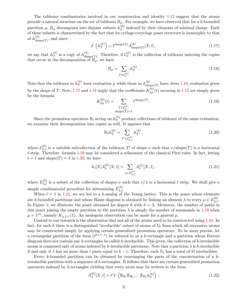
The tableaux combinatorics involved in our construction and identity 1.12 suggest that the atomsprovide a natural structure on the set of tableaux Hµ. For example, we have observed that for a k-boundedpartition µ, Hµ decomposes into disjoint subsets A(k)

T indexed by their elements of minimal charge. Eachof these subsets is characterized by the fact that its cyclage-cocyclage poset structure is isomorphic to thatof A(k)

shape(T ), and since

z(A(k)

T

)= tcharge(T )A

(k)shape(T )[X; t] , (1.17)

we say that A(k)T is a copy of A(k)

shape(T ). Therefore, if C(k)µ is the collection of tableaux indexing the copies

that occur in the decomposition of Hµ, we have

Hµ =∑

T∈C(k)µ

A(k)T . (1.18)

Note that the tableaux in A(k)T have evaluation µ while those in A(k)

shape(T ) have, from 1.10, evaluation given

by the shape of T . Now, 1.17 and 1.18 imply that the coefficients K(k)λµ (t) occuring in 1.12 are simply given

by the formulaK

(k)λµ (t) =

∑T∈C(k)

µ

shape(T )=λ

tcharge(T ) . (1.19)

Since the promotion operators B` acting on A(k)T produce collections of tableaux of the same evaluation,

we examine their decomposition into copies as well. It appears that

B`A(k)T =

∑T ′∈E(k)

T,`

A(k)T ′ , (1.20)

where E(k)T,` is a suitable subcollection of the tableaux T ′ of shape ν such that ν/shape(T ) is a horizontal

`-strip. Therefore, formula 1.20 may be considered a refinement of the classical Pieri rules. In fact, lettingt = 1 and shape(T ) = λ in 1.20, we have

h`[X]A(k)λ [X; 1] =

∑ν∈E

(k)λ,`

A(k)ν [X; 1] , (1.21)

where E(k)λ,` is a subset of the collection of shapes ν such that ν/λ is a horizontal ` strip. We shall give a

simple combinatorial procedure for determining E(k)λ,` .

When ` = 1 in 1.21, we are led to a k-analog of the Young lattice. This is the poset whose elementsare k-bounded partitions and whose Hasse diagram is obtained by linking an element λ to every µ ∈ E

(k)λ,1.

In Figure 1, we illustrate the poset obtained for degree 6 with k = 3. Moreover, the number of paths inthis poset joining the empty partition to the partition λ is simply the number of summands in 1.19 whenµ = 1|λ|, namely Kλ,1|λ|(1). An analogous observation can be made for a general µ.

Central to our research is the observation that not all of the atoms need to be constructed using 1.10. Infact, for each k there is a distinguished ”irreducible” subset of atoms of Vk from which all successive atomsmay be constructed simply by applying certain generalized promotion operators. To be more precise, leta rectangular partition of the form (`k+1−`) be referred to as a k-rectangle and a partition whose Ferrersdiagram does not contain any k-rectangles be called k-irreducible. This given, the collection of k-irreducibleatoms is composed only of atoms indexed by k-irreducible partitions. Note that a partition λ is k-irreducibleif and only if λ has no more than i parts equal to k − i. Therefore, each Vk has a total of k! irreducibles.

Every k-bounded partition can be obtained by rearranging the parts of the concatenation of a k-irreducible partition with a sequence of k-rectangles. It follows that there are certain generalized promotionoperators indexed by k-rectangles yielding that every atom may be written in the form

A(k)λ [X; t] = tcz

(BR1BR2 . . . BR`

A(k)µ

), (1.22)

3

......................................

.......................................................................................................

...................................................................................................

..................................................................................................

........................................................................................

......................................................................................................

..............................................................................................

......................................................................................................

..............................................................................................

.................................................................................................

.............................................................................................

..........................................................................................

....................................................................................................

...............................................................................................

............................................................................................

............................................................................................

..............................................................................................

...........................................................................................................................

.......................................................................................................................................................................................................... ......................................

.........................................................................................

...................................................................................................

...............................................................................................

................................................................................................................................................................................................................................................................... ......................................

.......................................................................................................

................................................................................................

..................................................................................

..................................................................................

.....................................................................................................................................................

...............................................................................................................

1

2

1,1,12,1

3,1 2,2 2,1,1 1,1,1,1

3,2 3,1,1 2,2,1 2,1,1,1 1,1,1,1,1

0

3,2,1 3,1,1,1 2,2,2 2,2,1,1 2,1,1,1,1 1,1,1,1,1,13,3

1,1

3

Figure 1: 3-analog of the Young Lattice

where µ is a k-irreducible partition, R1, . . . , R` are certain k-rectangles, and c ∈ N.Again we find it interesting to consider the case t = 1. First, since the Hall-Littlewood polynomials at

t = 1 are simplyH(µ1,...,µn)[X; 1] = hµ1 [X] · · ·hµn [X] , (1.23)

we see that Vk reduces to the polynomial ring Vk(1) = Q[h1, . . . , hk]. Further, since the construction in1.22 is simply multiplication by Schur functions when t = 1,

A(k)λ [X; 1] = SR1 [X]SR2 [X] . . . SR`

[X]A(k)µ [X; 1] , (1.24)

it thus follows that k-irreducible atoms constitute a natural basis for the quotient Vk(1)/Ik, where Ik isthe ideal generated by Schur functions indexed by k-rectangles. In fact, the irreducible atom basis offers avery beautiful way to carry out operations in this quotient ring: first work in Vk(1) using atoms and thenreplace by zero all atoms indexed by partitions which are not k-irreducible.

We shall examine our k-analog of the Young lattice restricted to k-irreducible partitions. Figure 5 givesthe case k = 3 and k = 4, where vertices denote irreducible atoms rather than partitions. Since it can beshown that the collection of monomials {hε1

1 , hε22 , . . . , hεk

k }0≤εi≤k−i forms a basis for the quotient Vk(1)/Ik,it follows that the Hilbert series FVk(1)/Ik

(q) of this quotient, as well as the rank generating function of thecorresponding poset, is given by

FVk(1)/Ik(q) =

k−1∏i=1

(1 + qi + q2i + · · ·+ q(k−i)i

). (1.25)

Finally, we shall make connections between our work and contemporary research in this area. Wediscovered that tableaux manipulations similar to ours have been used for a different purpose in [15]. Inparticular, we believe certain cases of the generalized Kostka polynomials can be expressed in our notationas

z (BR1 · · ·BR`H0) , (1.26)

where R1, . . . , R` is a sequence of rectangles whose concatenation is a partition. When R1, . . . , R` isa sequence of k-rectangles this is simply the case µ = ∅ in 1.22. Thus, it is again apparent that an

4

integral part of our work lies in the k-irreducible atoms, without which the atoms in general could not beconstructed.

Furthermore, it is known that these generalized Kostka polynomials can be built from the symmetricfunction operators BR introduced in [16]. The connection we have made with our atoms and these poly-nomials thus suggest that any atom can be obtained by applying a succesion of operators BR indexed byk-rectangles to a given irreducible atom A

(k)µ [X; t]:

A(k)λ [X; t] = tcBR1BR2 · · ·BR`

A(k)µ [X; t] , where c ∈ N . (1.27)

Note this is a symmetric function analog of 1.22 and specializes to 1.24 when t = 1.

Acknowledgments. We give our deepest thanks to Adriano Garsia for all his time and effort helping usarticulate our ideas. Our research depended on the use of ACE [17].

2 Background

2.1 Symmetric function theory

Here symmetric functions are indexed by partitions, or sequences of non-negative integers λ = (λ1, λ2, . . .)with λ1 ≥ λ2 ≥ . . . . The order of λ is |λ| = λ1 + λ2 + . . . , the number of non-zero parts in λ is denoted`(λ), and n(λ) =

∑i(i− 1)λi. We use the dominance order on partitions with |λ| = |µ|, where λ ≤ µ when

λ1 + · · · + λi ≤ µ1 + · · · + µi for all i. Every partition λ may be associated to a Ferrers diagram with λi

lattice squares in the ith row, from the bottom to top. For example,

λ = (4, 3, 1) = . (2.1)

For each cell s = (i, j) in the diagram of λ, let `′(s), `(s), a(s), and a′(s) be respectively the number ofcells in the diagram of λ to the south, north, east, and west of the cell s. The transposition of a diagramassociated to λ with respect to the main diagonal gives the conjugate partition λ′. For example, theconjugate of (4,3,1) is

λ′ = = (3, 2, 2, 1) . (2.2)

A skew diagram µ/λ, for any partition µ containing the partition λ, is the diagram obtained by deletingthe cells of λ from µ. The thick frames below represent (5,3,2,1)/(4,2).

. (2.3)

We employ the notation of λ-rings, needing only the formal ring of symmetric functions Λ to act onthe ring of rational functions in x1, . . . , xN , q, t, with coefficients in Q. The action of a power sum pi on arational function is, by definition,

pi

[∑α cαuα∑β dβvβ

]=∑

α cαuiα∑

β dβviβ

, (2.4)

with cα, dβ ∈ Q and uα, vβ monomials in x1, . . . , xN , q, t. Since the ring Λ is generated by power sums, pi,any symmetric function has a unique expression in terms of pi, and 2.4 extends to an action of Λ on rationalfunctions. In particular f [X], the action of a symmetric function f on the polynomial X = x1 + · · ·+ xN ,is simply f(x1, . . . , xN ).

We recall that the Macdonald scalar product, 〈 , 〉q,t, on Λ⊗Q[q, t] is defined by setting

〈pλ[X], pµ[X]〉q,t = δλµ zλ

`(λ)∏i=1

1− qλi

1− tλi= δλµ zλ pλ

[1− q

1− t

], (2.5)

5

where for a partition λ with mi(λ) parts equal to i, we associate the number

zλ = 1m1m1! 2m2m2! · · · (2.6)

The Macdonald integral forms Jλ[X; q, t] are then uniquely characterized [10] by

(i) 〈Jλ, Jµ〉q,t = 0, if λ 6= µ, (2.7)

(ii) Jλ[X; q, t] =∑µ≤λ

vλµ(q, t)Sµ[X], (2.8)

(iii) vλλ(q, t) =∏s∈λ

(1− qa(s)t`(s)+1), (2.9)

where Sµ[X] is the usual Schur function and vλµ(q, t) ∈ Q[q, t].

2.2 Tableaux combinatorics

A∗ denotes the free monoid generated by the alphabet A = {1, 2, . . .} and Q[A∗] is the free algebra of A.Elements of A∗ are called words and for E a subset of A, wE denotes the subword obtained by removingfrom w all the letters not in E. The degree of a word w is denoted |w| and if w has ρ1 ones, ρ2 twos, . . .,and ρm m’s, then the evaluation of w is ev(w)=(ρ1, . . . , ρm). For example, w = 131332 has degree 6 andevaluation (2,1,3). We use eva(w) for the multiplicity of letter a in the word w. A word w of degree n isstandard iff ev(w)=(1, . . . , 1). Recall that a word w is Yamanouchi in the letters a1 <. . .<ah if it is suchthat for every factoring w = uv, v contains more ai than aj for all i<j.

The plactic monoid on the alphabet A is the quotient A∗/ ≡, where ≡ is the congruence generated bythe Knuth relations [4] defined on three letters a, b, c by

a c b ≡ c a b (a ≤ b < c) ,

b a c ≡ b c a (a < b ≤ c) . (2.10)

Two words w and w′ are said to be Knuth equivalent iff w ≡ w′.In this paper, a tableau is a filling of a Ferrers diagram with positive integer entries that are nonde-

creasing in rows and increasing in columns:

T = 6 74 4 51 1 1 2 3

. (2.11)

The word w obtained by reading the entries of a tableau from left to right and top to bottom is said to bea tableau word, or simply a tableau. Our example shows that w = 6744511123 is a tableau with evaluation(3,1,1,2,1,1,1). A standard tableau T is a tableau of evaluation (1, 1, . . . , 1). For example,

T = 74 61 2 3 5

. (2.12)

The transpose of a standard tableaux T t is defined in the same manner as the transpose of a Ferrersdiagram. With T as given in 2.12, we have

T t =532 61 4 7

. (2.13)

Since the transpose of a tableau is assured to be a tableau only when the original tableau is standard, thisdefinition is valid only for standard tableaux.

We assume readers are familiar with the Robinson-Schensted correspondence [11, 12],

w ←→(P (w), Q(w)

), (2.14)

6

providing a bijection between a word w and a pair of tableaux(P (w), Q(w)

), where P (w) is the only

tableau Knuth equivalent to w and Q(w) is a standard tableau.The ring of symmetric functions is embedded into the plactic algebra by sending the Schur function

Sλ to the sum of all tableaux of shape λ [1, 7]. The commutativity of the product SλSµ ≡ SµSλ thusimplies bijections among tableaux. In particular, we can define the following action of the symmetricgroup on words [9]. The elementary transposition σi permutes degrees in i and i + 1. Given a word wof evaluation (ρ1, . . . , ρm), let u denote the subword in letters a = i and b = i + 1. The action of thetransposition σi affects only the subword u and is defined as follows: pair every factor b a of u, and letu1 be the subword of u made out of the unpaired letters. Pair every factor b a of u1, and let u2 be thesubword made out of the unpaired letters. When all factors b a are paired and unpaired letters of u are ofthe form arbs, σi sends arbs → asbr. For instance, to obtain the action of σ2 on w = 123343222423, wehave u = w{2,3} = 233322223, and the pairings are

2(3(3(32)2

)2)23 , (2.15)

which means that σ2u = 233322233 and σ2w = 123343222433. It is verified in [9] that the σi’s obey theCoxeter relations and thus provide an action of the symmetric group on words.

We use the notion of charge [7, 8] defined by writing a word w, with evaluation given by a partition,counterclockwise on a circle with a * separating the end of the word from its begining and then summingthe labels that are obtained by the following procedure:

1. Moving clockwise, label the first unlabelled i := 1 with c := 0 (if there are no unlabelled i = 1, theprocedure is over). Let i := i + 1.

2. If all i are labelled then go to step 1. Else, the next unlabelled i is labelled with c := c if i occursbefore crossing * and otherwise with c := c + 1. Let i := i + 1 and repeat step 2.

We can define charge on a word w whose evaluation is not a partition by first permuting the evaluationto a partition using σ, and then taking the charge of σw. Figure 2 shows that charge(12114123234) =

Figure 2: Charge of w = 12114123234

0 + 0 + 0 + 0 + 1 + 0 + 1 + 1 + 1 + 1 + 2 = 7.The definition of charge gives that a tableau of shape and evaluation µ has charge 0 and thus the

combinatorial construction for the Hall-Littlewood polynomials (1.6) implies

Hλ[X; t] = Sλ[X] +∑µ>λ

Kµλ(0, t)Sµ[X] . (2.16)

7

3 Definition of A(k)λ [X; t]

Our main contribution is the method for constructing new families of functions whose significance hasbeen outlined in the introduction. The characterization is similar to the combinatorial definition of Hall-Littlewood polynomials using the set of tableaux that arises from a recursive application of promotionoperators. Our families also correspond to a set of tableaux generated by the promotion operators, buthere we introduce new operators Pλ→k to eliminate undesirable elements. To be precise, we now define theoperators involved in our construction.

The promotion operators are defined on a tableau T with evaluation (λ1, . . . , λm) by

Br : T −→ σ1 · · ·σm Rr T , (3.1)

where Rr adds a horizontal r-strip of the letter m + 1 to T in all possible ways. For example,

B32 21 1

= σ1 σ2 R32 21 1

= σ1σ2

(2 21 1 3 3 3

+ 32 21 1 3 3

+ 3 32 21 1 3

)= 2 2

1 1 1 3 3+ 3

2 21 1 1 3

+ 3 32 21 1 1

.

Note that the action of σ implies that the resulting tableaux have evaluation (r, λ1, . . . , λm). While ourconstruction relies on these operators, they generate certain unwanted tableaux. We now present theconcepts needed to obtain operators that filter out such elements.

The main hook-length of a partition λ, hM (λ), is the hook-length of the cell s = (1, 1) in the diagramassociated to λ. That is

hM (λ) = `(s) + a(s) + 1 = λ1 + λ′1 − 1 = λ1 + `(λ)− 1 . (3.2)

For example, if λ = (4, 3, 1), thenhM (λ) =

••• • • •

= 6 . (3.3)

Any k-bounded partition λ can be associated to a sequence of partitions called the k-split, λ→k =(λ(1), λ(2), . . . , λ(r)). The k-split of λ is obtained by dividing λ (without changing the order of its entries)into partitions λ(i) where hM (λ(i)) = k, ∀ i 6= r. For example, (3, 2, 2, 2, 1, 1)→3 =

((3), (2, 2), (2, 1), (1)

).

Equivalently, we horizontally cut the diagram of λ into partitions λ(i) where hM (λ(i)) = k. In our examplethis gives

−→. (3.4)

Note, the last partition in the sequence λ→k may have main hook-length less than k. As k increases, thek-split of λ will contain fewer partitions. For k = 4,

−→ or (3, 2, 2, 2, 1, 1)→4 =((3, 2), (2, 2, 1), (1)

). (3.5)

When k is big enough (hM (λ) ≤ k), then λ→k =(λ). i.e., (3, 2, 2, 2, 1, 1)→8 =((3, 2, 2, 2, 1, 1)

).

Let T be a given tableau whose shape contains λ. We shall denote by Tλ, the subtableau of T of shapeλ. Let U be the skew tableau obtained by removing Tλ from T , let T1 be the tableau contained in the first`(λ) rows of U , and T2 be the portion of U that is above the `(λ) rows. Let us denote by T1T2 the skewtableau obtained by juxtaposing T1 to the northwest corner of T2, and by T the unique tableau which isKnuth equivalent to T1T2. For instance, in the figure below λ = (3, 2, 1, 1), the skew tableau with empty

8

cells is T1, the tableau with bullets is T2, the middle diagram is T1T2, and the right diagram is a possibleshape for T .

•• •• • • • −→

•• •• • • •

≡ . (3.6)

This construction permits us to define an operation on tableau, Kλ, called λ-katabolism.

Kλ : T −→{

T if λ ⊆ shape(T )0 otherwise

.

For example, the (2, 1)-katabolism of T = 9472581236 is

K(2,1)

94 72 5 81 2 3 6

−→5 8

3 694 7

≡ 85 6 93 4 7

. (3.7)

Note that λ-katabolism was also introduced in [15] and for the case that λ is a row, in [9].Let S(λ) be the set of λ-shaped tableaux with evaluations (0m, λ1, λ2, . . .), for m ∈ N. For λ = (3, 2, 2),

we haveS

( )={

3 32 21 1 1

,4 43 32 2 2

,5 54 43 3 3

,6 65 54 4 4

, . . .

}. (3.8)

This given, the restricted λ-katabolism Kλ is defined by setting

Kλ : T −→{

Kλ(T ) if Tλ ∈ S(λ)0 otherwise

. (3.9)

For example, K(2,1) on the tableau in 3.7 is zero, whereas

K(2,1)

94 72 5 81 1 3 6

=

5 83 6

94 7

≡85 6 93 4 7

. (3.10)

For a sequence of partitions S = (λ(1), λ(2), . . . , λ(`)), we define the filtering operator PS using thesuccession of restricted katabolisms Kλ(`) · · ·Kλ(1) ,

PS : T −→{

T if Kλ(`) · · ·Kλ(1)(T ) = H0

0 otherwise. (3.11)

In fact, we only consider the case where S is the sequence of partitions given by λ→k.

Property 1. The filtering operators Pλ→k satisfy the following properties :a. For T ∈ S(λ), we have Pλ→kT = T for all k such that λ is bounded by k.b. For U a tableau of |λ| letters such that U 6∈ S(λ), Pλ→kU = 0 for all k ≥ hM (λ).

Proof. By definition 3.11, we must show Kλ(`) · · ·Kλ(1)T = H0, for λ→k = (λ(1), . . . , λ(`)). Recall thatKλ(1)T acts by extracting the bottom `(λ(1)) rows of T and inserting into the remainder, any entries notin Tλ(1) ∈ S(λ(1)). Since the bottom `(λ(1)) rows of T ∈ S(λ) are exactly Tλ(1) ∈ S(λ(1)), the katabolismKλ(1)T simply removes the bottom `(λ(1)) rows of T . By iteration, we obtain the empty tableau.

For (b), the condition that k is large implies that λ→k = (λ). It thus suffices to show that Kλ(U) = 0.Now Kλ acts first by extracting from U , the subtableau Uλ ∈ S(λ). If U is of shape λ then Uλ = U 6∈ S(λ).If U is not of shape λ, since U has degree |λ|, then Uλ does not exist. Therefore we have our claim. �

These filtering operators are those required in the characterization of our families of functions. We thushave the tools to recursively define the central object in our work, the super atom of shape λ and level k,A(k)

λ .

9

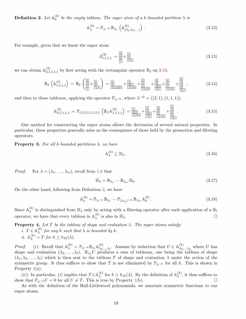
Definition 2. Let A(k)0 be the empty tableau. The super atom of a k-bounded partition λ is

A(k)λ = Pλ→k Bλ1

(A(k)

(λ2,λ3,... )

). (3.12)

For example, given that we know the super atom

A(3)1,1,1,1 =

4321

+ 321 4

(3.13)

we can obtain A(3)2,1,1,1,1 by first acting with the rectangular operator B2 on 3.13,

B2

(A(3)

1,1,1,1

)= B2

(4321

+ 321 4

)= 3

21 1 4 5

+ 32 51 1 4

+5321 1 4

+432 51 1

+4321 1 5

+54321 1

, (3.14)

and then to these tableaux, applying the operator Pλ→k , where λ→k =((2, 1), (1, 1, 1)

);

A(3)2,1,1,1,1 = P((2,1),(1,1,1))

(B2 A(3)

1,1,1,1

)= 3

2 51 1 4

+432 51 1

+4321 1 5

+54321 1

. (3.15)

Our method for constructing the super atoms allows the derivation of several natural properties. Inparticular, these properties generally arise as the consequence of those held by the promotion and filteringoperators.

Property 3. For all k-bounded partitions λ, we have

A(k)λ ⊆ Hλ . (3.16)

Proof. For λ = (λ1, . . . , λm), recall from 1.8 that

Hλ = Bλ1 · · ·Bλm H0 . (3.17)

On the other hand, following from Definition 2, we have

A(k)λ = Pλ→k Bλ1 · · ·P(λm)→k Bλm A(k)

0 . (3.18)

Since A(k)λ is distinguished from Hλ only by acting with a filtering operator after each application of a B`

operator, we have that every tableau in A(k)λ is also in Hλ. �

Property 4. Let T be the tableau of shape and evaluation λ. The super atoms satisfy:i. T ∈ A(k)

λ for any k such that λ is bounded by k.ii. A(k)

λ = T for k ≥ hM (λ).

Proof. (i): Recall that A(k)λ = Pλ→kBλ1A

(k)λ2,...,λ`

. Assume by induction that U ∈ A(k)λ2,...,λ`

where U hasshape and evaluation (λ2, . . . , λ`). Rλ1U produces a sum of tableaux, one being the tableau of shape(λ1, λ2, . . . , λ`) which is then sent to the tableau T of shape and evaluation λ under the action of thesymmetric group. It thus suffices to show that T is not eliminated by Pλ→k for all k. This is shown inProperty 1(a).

(ii): In particular, (i) implies that T ∈A(k)λ for k ≥ hM (λ). By the definition of A(k)

λ , it thus suffices toshow that Pλ→kU = 0 for all U 6= T . This is true by Property 1(b). �

As with the definition of the Hall-Littlewood polynomials, we associate symmetric functions to oursuper atoms.

10

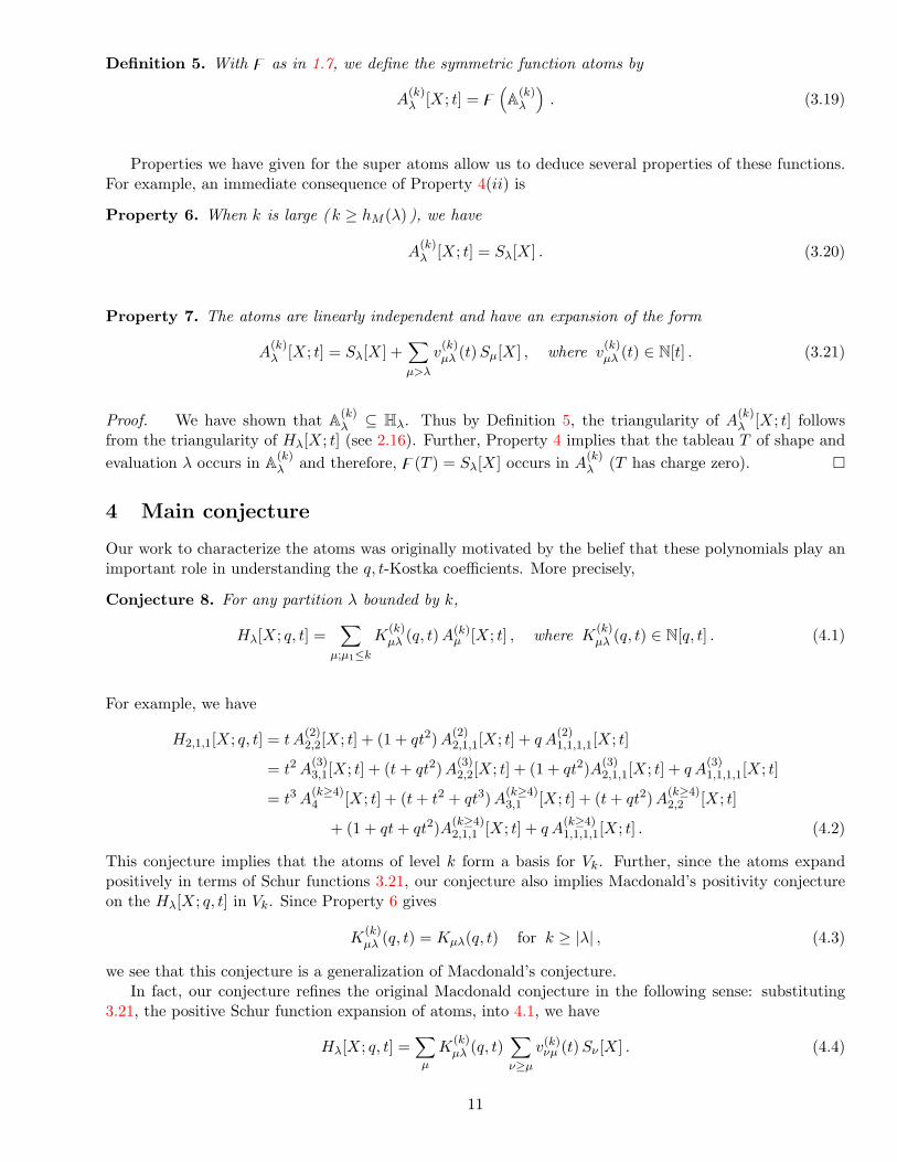
Definition 5. With z as in 1.7, we define the symmetric function atoms by

A(k)λ [X; t] = z

(A(k)

λ

). (3.19)

Properties we have given for the super atoms allow us to deduce several properties of these functions.For example, an immediate consequence of Property 4(ii) is

Property 6. When k is large ( k ≥ hM (λ) ), we have

A(k)λ [X; t] = Sλ[X] . (3.20)

Property 7. The atoms are linearly independent and have an expansion of the form

A(k)λ [X; t] = Sλ[X] +

∑µ>λ

v(k)µλ (t) Sµ[X] , where v

(k)µλ (t) ∈ N[t] . (3.21)

Proof. We have shown that A(k)λ ⊆ Hλ. Thus by Definition 5, the triangularity of A

(k)λ [X; t] follows

from the triangularity of Hλ[X; t] (see 2.16). Further, Property 4 implies that the tableau T of shape andevaluation λ occurs in A(k)

λ and therefore, z(T ) = Sλ[X] occurs in A(k)λ (T has charge zero). �

4 Main conjecture

Our work to characterize the atoms was originally motivated by the belief that these polynomials play animportant role in understanding the q, t-Kostka coefficients. More precisely,

Conjecture 8. For any partition λ bounded by k,

Hλ[X; q, t] =∑

µ;µ1≤k

K(k)µλ (q, t) A(k)

µ [X; t] , where K(k)µλ (q, t) ∈ N[q, t] . (4.1)

For example, we have

H2,1,1[X; q, t] = t A(2)2,2[X; t] + (1 + qt2) A

(2)2,1,1[X; t] + q A

(2)1,1,1,1[X; t]

= t2 A(3)3,1[X; t] + (t + qt2) A

(3)2,2[X; t] + (1 + qt2)A(3)

2,1,1[X; t] + q A(3)1,1,1,1[X; t]

= t3 A(k≥4)4 [X; t] + (t + t2 + qt3) A

(k≥4)3,1 [X; t] + (t + qt2) A

(k≥4)2,2 [X; t]

+ (1 + qt + qt2)A(k≥4)2,1,1 [X; t] + q A

(k≥4)1,1,1,1[X; t] . (4.2)

This conjecture implies that the atoms of level k form a basis for Vk. Further, since the atoms expandpositively in terms of Schur functions 3.21, our conjecture also implies Macdonald’s positivity conjectureon the Hλ[X; q, t] in Vk. Since Property 6 gives

K(k)µλ (q, t) = Kµλ(q, t) for k ≥ |λ| , (4.3)

we see that this conjecture is a generalization of Macdonald’s conjecture.In fact, our conjecture refines the original Macdonald conjecture in the following sense: substituting

3.21, the positive Schur function expansion of atoms, into 4.1, we have

Hλ[X; q, t] =∑µ

K(k)µλ (q, t)

∑ν≥µ

v(k)νµ (t) Sν [X] . (4.4)

11

On the other hand, since the q, t-Kostka coefficients appear in the expansion

Hλ[X; q, t] =∑ν

Kνλ(q, t) Sν [X] , (4.5)

we have that

Kνλ(q, t) =∑µ≤ν

K(k)µλ (q, t) v(k)

νµ (t)

= K(k)νλ (q, t) +

∑µ<ν

K(k)µλ (q, t) v(k)

νµ (t) . (4.6)

Since v(k)νµ (t) is in N[q, t], Conjecture 8 implies that

K(k)µλ (1, 1) ≤ Kµλ(1, 1) , (4.7)

where Kµλ(1, 1) is known to be the number of standard tableaux of shape µ. Thus, the problem of findinga combinatorial interpretation for the Kµλ(q, t) coefficients (i.e. associating statistics to standard tableaux)is reduced to obtaining statistics for the fewer K

(k)µλ (q, t). We do not address this problem here, but the

the complete solution of Conjecture 8 for k = 2 is given in [5, 15, 18].Based on our conjecture, we have the following corollary concerning the expansion of Hall-Littlewood

polynomials in terms of our atoms.

Corollary 9. For any partition λ bounded by k,

Hλ[X; t] =∑µ≥λ

K(k)µλ (t) A(k)

µ [X; t] where K(k)µλ (t) ∈ N[t] . (4.8)

If we consider this corollary as the result of applying z to an identity on tableaux,

z (Hλ) =∑µ

K(k)µλ (t) z

(A(k)

µ

), where Kµλ(t) ∈ N[t] , (4.9)

then it is suggested that the set of all tableaux with evaluation λ can naturally be decomposed into subsetsthat are mapped under z to the atoms A

(k)µ [X; t]. Here, K

(k)µλ (1) corresponds to the number of times such

a subset occurs in Hλ which, by 4.6, is such that

K(k)µλ (1) ≤ Kµλ(1) , (4.10)

where Kµλ(1) is the number of tableaux with evaluation λ and shape µ. These subsets will be called copiesof A(k)

µ and they will provide a natural decomposition for the set of tableaux of a given evaluation.

5 Embedded tableaux decomposition

It is suggested from 4.9 that the set of all tableaux with given evaluation can be decomposed into subsetsassociated to our super atoms. These subsets will be characterized by a cyclage-cocyclage ranked-posetstructure [9].

For tableau T =xw where x is not the smallest letter of T , we define T ′ to be the unique tableau suchthat T ′ ≡ wx. The mapping T → T ′ is a called a cyclage and is such that charge(T ′) = charge(T ) + 1. Fortableau T = wx where x is not the smallest letter of T , we define T ′ to be the unique tableau such thatT ′ ≡ xw. The cocyclage is the mapping T → T ′ and is such that charge(T ′) = charge(T )− 1.

On any collection of tableaux T of the same evaluation, we can define the poset (T, <cc) by linking anytwo tableaux T and T ′ if T is obtained from T ′, or vice versa, using either a cyclage or a cocyclage. This

12

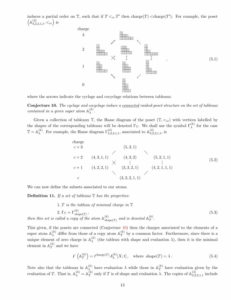
induces a partial order on T, such that if T <cc T ′ then charge(T ) <charge(T ′). For example, the poset(A(4)

3,2,2,1,1, <cc

)is

charge3 3

2 2 51 1 1 3 4

↙↗ ↖

2432 2 51 1 1 3

3 32 2 51 1 1 4

432 21 1 1 3 5

↘↗ l l

143 32 21 1 1 5

43 32 2 51 1 1

5432 21 1 1 3

↘↖ ↙

0543 32 21 1 1

, (5.1)

where the arrows indicate the cyclage and cocyclage relations between tableaux.

Conjecture 10. The cyclage and cocyclage induce a connected ranked-poset structure on the set of tableauxcontained in a given super atom A(k)

λ .

Given a collection of tableaux T, the Hasse diagram of the poset (T, <cc) with vertices labelled bythe shapes of the corresponding tableaux will be denoted ΓT. We shall use the symbol Γ(k)

λ for the caseT = A(k)

λ . For example, the Hasse diagram Γ(4)3,2,2,1,1, associated to A(4)

3,2,2,1,1, is

chargec + 3 (5, 3, 1)

� �c + 2 (4, 3, 1, 1) (4, 3, 2) (5, 2, 1, 1)

�� | |c + 1 (4, 2, 2, 1) (3, 3, 2, 1) (4, 2, 1, 1, 1)

� �c (3, 2, 2, 1, 1)

(5.2)

We can now define the subsets associated to our atoms.

Definition 11. If a set of tableaux T has the properties:

1. T is the tableau of minimal charge in T

2. ΓT = Γ(k)shape(T ) , (5.3)

then this set is called a copy of the atom A(k)shape(T ) and is denoted A(k)

T .

This given, if the posets are connected (Conjecture 10) then the charges associated to the elements of asuper atom A(k)

λ differ from those of a copy atom A(k)T by a common factor. Furthermore, since there is a

unique element of zero charge in A(k)λ (the tableau with shape and evaluation λ), then it is the minimal

element in A(k)T and we have

z(A(k)

T

)= tcharge(T )A

(k)λ [X; t] , where shape(T ) = λ . (5.4)

Note also that the tableaux in A(k)λ have evaluation λ while those in A(k)

T have evaluation given by theevaluation of T . That is, A(k)

λ = A(k)T only if T is of shape and evaluation λ. The copies of A(4)

3,2,2,1,1 include

13

A(4)863925147, given by

charge13 3

2 5 71 4 6 8 9

↙↗ ↖

12932 5 71 4 6 8

3 92 5 71 4 6 8

632 51 4 7 8 9

↘↗ l l

1163 92 51 4 7 8

83 92 5 71 4 6

9632 51 4 7 8

↘↖ ↙

10863 92 51 4 7

(5.5)

It appears that there is a unique way to decompose the set of all tableaux Hµ into atoms of level k ≥ µ1.More precisely, we let C(k)

µ denote the collection of all tableaux T with evaluation µ where A(k)T is a copy

of a super atom of level k. Then

Conjecture 12. For any partition µ bounded by k, we have

Hµ =∑

T∈C(k)µ

A(k)T . (5.6)

From Corollary 9 and 5.4, an implication of this identity under the mapping z is:

Corollary 13. The k-Kostka-Foulkes polynomials are simply

K(k)λµ (t) =

∑T∈C(k)

µ

shape(T )=λ

tcharge(T ) . (5.7)

One method to obtain the set C(k)µ is as follows: The element of minimal charge in Hµ has shape µ

and is thus also the minimal element of A(k)µ . Remove from Hµ, all tableaux in A(k)

µ . Choose a tableau T

with minimal charge from those that remain. T must index a copy of the atom A(k)λ where λ = shape(T ).

>From the Hasse diagram Γ(k)λ , it is possible to find and remove all tableaux in the atom A(k)

T . Repeat thisprocedure always on an element of minimal charge in the resulting sets. The collection of these minimalelements is C(k)

µ .Evidence suggests that this method also provides a direct decomposition of any copy atom of a level k

into copy atoms of level k′ > k.

Conjecture 14. For any atom A(k)T such that shape(T ) is bounded by k, and any k′ > k,

A(k)T =

∑T ′∈D(k→k′)

T

A(k′)T ′ , (5.8)

for some collection of tableaux D(k→k′)T .

On the level of functions, this translates into

Corollary 15. If λ is a partition bounded by k, and k′ > k, then

A(k)λ [X; t] = A

(k′)λ [X; t] +

∑µ>λ

v(k→k′)µλ (t) A(k′)

µ [X; t] , where v(k→k′)µλ (t) ∈ N[t] . (5.9)

14

This conjecture is a generalization of the result presented in Property 7 since we recover v(k→k′)µλ (t) = vµλ(t)

when k′ ≥ |λ|.For examples that support the preceeding conjectures, refer to Figures 6 and 7. These figures also

suggest that the number of elements in an atom, at increasing charges, forms a unimodal sequence. Sincean atom has a unique minimal element, these sequences always start with 1.

Conjecture 16. Given any atom

A(k)λ [X; t] =

∑µ≥λ

v(k)µλ (t) Sµ[X; t] , (5.10)

the numbers#i =

∑µ≥λ

v(k)µλ (t)

∣∣∣ti

, (5.11)

are such that [#0,#1, . . . ] is a unimodal sequence.

For example, the unimodal sequence associated to A(4)3,2,2,1,1,1[X; t] is [1, 3, 5, 5, 3, 1]:

A(4)3,2,2,1,1,1[X; t] = S3,2,2,1,1,1 + t S4,2,1,1,1,1 + t S3,3,2,1,1 +

(t + t2

)S4,2,2,1,1 + t2 S3,3,3,1

+ t2 S4,3,1,1,1 +(t2 + t3

)S5,2,1,1,1 +

(t2 + t3

)S4,3,2,1 + t3 S5,2,2,1

+ t3 S4,3,3 +(t3 + t4

)S5,3,1,1 + t4 S6,2,1,1 + t4 S5,3,2 + t5 S6,3,1 . (5.12)

We will see later (Corollary 37) that these sequences also end with a one, that is an atom has a uniqueelement of maximal charge. We will provide a way to obtain the shape of this maximal element.

We finish this section by stating a conjecture that reiterates the importance of the atoms as a naturalbasis for Vk.

Conjecture 17. For any two alphabets X and Y ,

A(k)λ [X + Y ; t] =

∑|µ|+|ρ|=|λ|

gλµρ(t) A(k)

µ [X; t]A(k)ρ [Y ; t] , (5.13)

with gλµρ(t) ∈ N[t].

It is important to note that the positivity of the coefficients gλµρ(t) appearing here is a natural property

of Schur functions that is not shared by the Hall-Littewood or Macdonald functions.

6 Irreducible atoms

We have now seen that the super atoms can be constructed by generating sets of tableaux with promotionoperators Br and then eliminating undesirable elements using the projection operators Pλ→k . Further, wehave given a method to obtain copies of the super atoms allowing us to decompose the set of all tableauxwith a given evaluation and to provide natural properties on the functions A

(k)λ [X; t].

Remarkably, it appears that there is a method to construct many of the atoms without generating anyundesirable elements. In fact, what could be seen as the ’DNA’ of our atoms is a subset of irreducibleatoms for each Vk, from which all successive atoms of Vk may be obtained by simply applying a generalizedversion of the promotion operators.

To be more precise, let a rectangular partition of the form (`k+1−`) be referred to as a k-rectangle anda partition whose Ferrers diagram does not contain any k-rectangles, that is with no more than i partsequal to k − i, be called k-irreducible.

Definition 18. The collection of k-irreducible atoms is composed of atoms indexed by k-irreducible parti-tions. If an atom is not irreducible, then it is said to be reducible.

15

Property 19. There are k! distinct k-irreducible partitions.

Proof. A partition λ is k-irreducible if and only if λ has no more than i parts equal to k − i. There areobviously k! such partitions. �The irreducible atoms of level 1,2 and 3 are

k = 1 : A(1)0 ,

k = 2 : A(2)0 , A

(2)1 ,

k = 3 : A(3)0 , A

(3)1 , A

(3)2 , A

(3)1,1 , A

(3)2,1 , A

(3)2,1,1 . (6.1)

The concatenation of λ and (`h) is obtained by adding h rows of length ` to λ:(λ + (`h)

)′ = (λ′1 + h, . . . , λ′` + h, λ′`+1, . . . ) . (6.2)

Any k-bounded partition µ can be obtained by a rearrangement of the concatenation of a k-irreduciblepartition with a sequence of k-rectangles. In fact, any atom of level k can be obtained from a k-irreducibleatom by the application of certain generalized promotion operators that are indexed by k-rectangles.

Before we can introduce these promotion operators, we need to define an operation which generalizesσi. We define σ

(h)i to send a word w of evaluation (ρ1, ρ2, . . . ) to a word w′ of evaluation

(ρ1, . . . , ρi−1, ρi+1, . . . , ρi+h, ρi, ρi+h+1, . . . ). The operation σ(h)i only acts on the subword w{i,...,i+h}, and

can thus be defined in generality from the special case i = 1. Let w be a word in 1, . . . , h + 1 and let(P (w), Q(w)

)denote the pair of tableaux in RS-correspondence with w (see 2.14). If w′′ is the word

obtained from w by first erasing all occurences of the letter 1 and then decreasing the remaining lettersby 1, then the shape of P (w′′) differs from that of P (w) by a horizontal strip. Let T ′ be the tableauobtained from P (w′′) by filling the horizontal strip with (h + 1)’s, and let w′ be the word which is inRS-correspondence with the pairs of tableaux

(P (w′), Q(w′)

)=(T ′, Q(w)

). We now define σ

(h)1 by setting

σ(h)1 : w → w′ . (6.3)

It can be shown that σ(1)i = σi, and thus σ

(h)i generalizes σi. Refer to [14] for a different generalization of

σi.The rectangular promotion operators are defined in a manner similar to the promotion operators. That

is, on a tableau T of evaluation (λ1, . . . , λm),

B(`h) : T −→ σ(h)1 · · ·σ

(h)m R(`h) T (6.4)

generates a sum of tableaux with evaluation (`h, λ1, . . . , λm) by applying a rectangular analog of Rr. Thisoperator, R(`h), acts by adding to T , a horizontal `-strip of the letter m+1, a horizontal `-strip of m+2,. . . ,and a horizontal `-strip of m + h in all possible ways such that the tableaux are Yamanouchi in the addedletters 6. Since σ

(1)i = σi for h = 1, we recover the previously defined promotion operator B`.

B(23)21 2

= σ(3)1 σ

(3)2 R(23)

21 2

= σ(3)1 σ

(3)2

5 52 4 41 2 3 3

+54 52 41 2 3 3

+5 54 42 31 2 3

+54 52 3 41 2 3

+543 52 41 2 3

+54 53 42 31 2

= 3 3

2 2 51 1 4 5

+43 32 21 1 5 5

+4 53 32 21 1 5

+53 32 2 51 1 4

+543 32 21 1 5

+54 53 32 21 1

. (6.5)

In fact, we believe that the inverse of the B(`h) action on an atom of level k is simply rectangular-katabolism,K(`h).

6 This is the multiplication involved in computing the Littlewood-Richardson coefficients in the product of a Schur functionof the shape of T by a Schur function indexed by a rectangular partition.

16

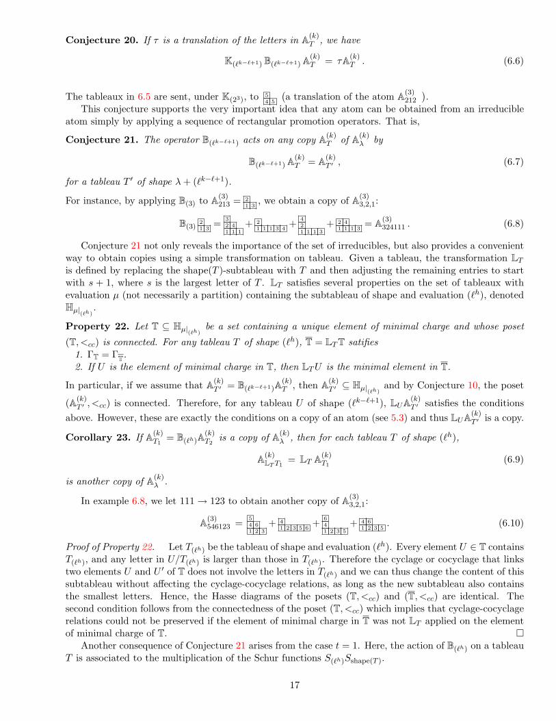
Conjecture 20. If τ is a translation of the letters in A(k)T , we have

K(`k−`+1) B(`k−`+1) A(k)T = τA(k)

T . (6.6)

The tableaux in 6.5 are sent, under K(23), to 54 5

(a translation of the atom A(3)

212

).

This conjecture supports the very important idea that any atom can be obtained from an irreducibleatom simply by applying a sequence of rectangular promotion operators. That is,

Conjecture 21. The operator B(`k−`+1) acts on any copy A(k)T of A(k)

λ by

B(`k−`+1) A(k)T = A(k)

T ′ , (6.7)

for a tableau T ′ of shape λ + (`k−`+1).

For instance, by applying B(3) to A(3)213 = 2

1 3, we obtain a copy of A(3)

3,2,1:

B(3)21 3

= 32 41 1 1

+ 21 1 1 3 4

+ 421 1 1 3

+ 2 41 1 1 3

= A(3)324111 . (6.8)

Conjecture 21 not only reveals the importance of the set of irreducibles, but also provides a convenientway to obtain copies using a simple transformation on tableau. Given a tableau, the transformation LT

is defined by replacing the shape(T )-subtableau with T and then adjusting the remaining entries to startwith s + 1, where s is the largest letter of T . LT satisfies several properties on the set of tableaux withevaluation µ (not necessarily a partition) containing the subtableau of shape and evaluation (`h), denotedHµ|

(`h).

Property 22. Let T ⊆ Hµ|(`h)

be a set containing a unique element of minimal charge and whose poset

(T, <cc) is connected. For any tableau T of shape (`h), T = LT T satifies1. ΓT = ΓT.2. If U is the element of minimal charge in T, then LT U is the minimal element in T.

In particular, if we assume that A(k)T ′ = B(`k−`+1)A

(k)T , then A(k)

T ′ ⊆ Hµ|(`h)

and by Conjecture 10, the poset

(A(k)T ′ , <cc) is connected. Therefore, for any tableau U of shape (`k−`+1), LUA(k)

T ′ satisfies the conditionsabove. However, these are exactly the conditions on a copy of an atom (see 5.3) and thus LUA(k)

T ′ is a copy.

Corollary 23. If A(k)T1

= B(`h)A(k)T2

is a copy of A(k)λ , then for each tableau T of shape (`h),

A(k)LT T1

= LT A(k)T1

(6.9)

is another copy of A(k)λ .

In example 6.8, we let 111→ 123 to obtain another copy of A(3)3,2,1:

A(3)546123 = 5

4 61 2 3

+ 41 2 3 5 6

+ 641 2 3 5

+ 4 61 2 3 5

. (6.10)

Proof of Property 22. Let T(`h) be the tableau of shape and evaluation (`h). Every element U ∈ T containsT(`h), and any letter in U/T(`h) is larger than those in T(`h). Therefore the cyclage or cocyclage that linkstwo elements U and U ′ of T does not involve the letters in T(`h) and we can thus change the content of thissubtableau without affecting the cyclage-cocyclage relations, as long as the new subtableau also containsthe smallest letters. Hence, the Hasse diagrams of the posets (T, <cc) and (T, <cc) are identical. Thesecond condition follows from the connectedness of the poset (T, <cc) which implies that cyclage-cocyclagerelations could not be preserved if the element of minimal charge in T was not LT applied on the elementof minimal charge of T. �

Another consequence of Conjecture 21 arises from the case t = 1. Here, the action of B(`h) on a tableauT is associated to the multiplication of the Schur functions S(`h)Sshape(T ).

17

Corollary 24. If we let A(k)λ = A

(k)λ [X; 1], then

S(`k−`+1) A(k)λ = A

(k)

λ+(`k−`+1). (6.11)

We have now seen that any atom can be understood as the application of rectangular promotionoperators to an irreducible component. Our study is thus reduced to examining the irreducibles (atoms oflevel k that cannot be obtained by applying k-rectangular operators to a smaller atom). Interestingly, wecan obtain the level k atom indexed by the irreducible partition of maximal degree,

λM =((k − 1)1, (k − 2)2, · · · , 1k−1) , (6.12)

by a recursive application of (k − 1)-rectangular promotion operators on the empty tableau.

Conjecture 25. The maximal irreducible atom of level k is an atom of level k − 1;

A(k)λM

[X; t] = A(k−1)λM

[X; t] . (6.13)

Furthermore, from Conjecture 21, this atom is simply

A(k)λM

[X; t] = A(k−1)λM

[X; t] = z(B(k−1)B((k−2)2) · · ·B(1k−1) H0

), (6.14)

For example, the atom A(3)2,1,1[X; t] is given by

A(3)2,1,1[X; t] = z

(B(2) B(12) H0

)= z

(321 1

+ 21 1 3

)= S2,1,1[X; t] + t S3,1[X; t] . (6.15)

When t = 1, Vk = {Hλ[X; t]}λ1≤k reduces to the polynomial ring Q[h1, . . . , hk] = Vk(1). If Ik denotesthe ideal generated by the k-rectangular Schur functions S(`k+1−`), we have the following proposition.

Proposition 26. The homogeneous functions indexed by k-irreducible partitions form a basis of the quo-tient ring Vk(1)/Ik.

Proof. For a partition λ bounded by k, we set

hλ =

{hλ if λ is k-irreduciblehµ+(`k+1−`) = S(`k+1−`) hµ if λ = µ + (`k+1−`)

. (6.16)

These elements are indexed by k-bounded partitions and thus, if independant, span a space with the samedimension as Vk(1). In fact, the hλ form a basis for Vk(1) since S(`k+1−`) = det (h`−i+j)1≤i,j≤k+1−` impliesthat hλ ∈ Vk(1); and Sλ = hλ +

∑µ>λ cµλhµ gives hλ = hλ +

∑µ>λ dµλhµ, which implies that they are

independant.First note that the hλ span the quotient ring Vk(1)/Ik because they span Vk(1). Since by definition

hµ ≡ 0 in the quotient ring when µ is not k-irreducible, the hλ indexed by k-irreducible partitions willform a basis for the quotient ring Vk(1)/Ik if they are independant in Vk(1)/Ik. Let S be the set of allk-irreducible partitions. If, in Vk(1)/Ik, we have∑

λ∈Sdλ hλ = 0 , (6.17)

then, in Vk(1), we must have ∑λ∈S

dλ hλ =∑

i

Ci S(ik+1−i) , (6.18)

18

for some Ci ∈ Vk(1). Further, since Ci =∑

µ ci,µhµ for some ci,µ, we have∑λ∈S

dλ hλ =∑i,µ

ci,µhµS(ik+1−i) =∑i,µ

ci,µhµ+(ik+1−i) . (6.19)

The basis elements appearing in the l.h.s of 6.19 are each indexed by k-irreducible partitions whereas thoseappearing in the r.h.s are indexed by non k-irreducible partitions. Therefore, dλ = 0 for all λ and by 6.17,this proves that the hλ indexed by k-irreducible partitions are independant in Vk(1)/Ik. �

We now have that the dimension of the quotient Vk(1)/Ik is k!. Since we assume that the atoms oflevel k form a basis for Vk, Corollary 24 implies that the k-irreducible atoms also form a basis of Vk(1)/Ik,since the atoms generate Vk(1)/Ik, and the only possibly non-zero atoms in Vk(1)/Ik are the k! irreducibleones.

Corollary 27. The k-irreducible atoms form a basis of the quotient ring Vk(1)/Ik.

If we link all atoms that occur in the action of e1 on a given atom in Vk(1)/Ik, we obtain a posetillustrated in Figure 5. The rank generating function of this poset was given in 1.25. This poset seems tohave a remarkable symmetry property called flip-invariance.

Definition 28. Given a k-irreducible partition of the form

λ =((k − 1)n1 , (k − 2)n2 , · · · , 1nk−1

)with ni ≤ i for all i , (6.20)

the involution called flip f(k) is defined by

f(k)A(k)λ = A

(k)

λf(k) (6.21)

where λf(k)=((k − 1)1−n1 , (k − 2)2−n2 , · · · , 1k−1−nk−1

). (6.22)

For instance,f(5)A

(5)4,3,2 = A

(5)3,2,2,1,1,1,1 .

Conjecture 29. The poset associated to the action of e1 on atoms in Vk(1)/Ik is flip-invariant. That is,if there is an arrow between two atoms A

(k)µ and A

(k)λ , then there will be an arrow between the two atoms

A(k)

µf(k) and A(k)

λf(k) .

Given the k! irreducible atoms, from which all other atoms are constructed using k-rectangular pro-motion operators, the complete decomposition of the standard tableaux into atoms can in principle beobtained. We give here the cases k = 2 and k = 3.

6.1 Case k = 2 and k = 3

Although the case k = 2 is given indirectly in [5, 15, 18], we briefly explain here how these results pertainto our work. If Sn denotes the set of standard tableaux on n letters, then(

B(2) + B(12)

)Sn = Sn+2 , (6.23)

where B(2) = L 21

B(2) and B(12) = B(12). This recursion implies, for A(2)0 = H0 and A(2)

1 = 1 ,

(B(2) + B(12)

)`A(2)

ε = S2`+ε , where ε ∈ {0, 1} . (6.24)

19

Expanding the right hand side gives∑(v1,...,vm)

B(v

3−v11 )

· · ·B(v3−vmm ) A(2)

ε = S2`+ε , for vi ∈ {1, 2} , (6.25)

and each of the standard tableau must occur in exactly one term of this sum. This is, each standardtableau must occur in exactly one family, denoted

A(2)(v1,...,vm,ε) = B

(v3−v11 )

· · ·B(v3−vmm ) A(2)

ε , vi ∈ {1, 2} . (6.26)

We have thus decomposed the set of standard tableaux into these families, which are the atoms of level 2by Conjecture 21 (which is a theorem for k = 2).

Now, lettingz(A(2)

(v1,...,vm,ε

)= t∗A

(2)λ [X; t] , (6.27)

where λ is the partition rearrangement of (v3−v11 , . . . , v3−vm

m , ε) and ∗ is a power of t. Furthermore, we canconnect the atoms to the Macdonald polynomials, since the creation operators that build the Macdonaldpolynomials recursively can be split into two operators B(2) and B(12) (the operators of section 6.2) suchthat,

B(v

3−v11 )

· · ·B(v3−vmm ) A(2)

ε [X; t] = t∗A(2)λ [X; t] . (6.28)

This allows us to give the expansion of Macdonald polynomials indexed by 2-bounded partitions (equiv-alently, partitions with `(λ) ≤ 2) into atoms of level 2. By Conjecture 8 (a theorem in this case), weassociate a (q, t)-statistic to each standard tableau. That is, given a standard tableau, we perform a (2)-katabolism if it contains the subword (12) and otherwise a (1,1)-katabolism. Repeating this procedure onthe resulting tableau, we obtain a sequence of vertical and horizontal 2-strips from which the (q, t)-statisticis determined.

In the case k = 3, we have the 8 irreducible atoms of 6 distinct shapes,

A(3)0 = H0 ; A(3)

1 = 1 ; A(3)12 = 1 2 ; A(3)

21 = 21

;

A(3)312 = 3

1 2; A(3)

213 = 21 3

; A(3)4312 = 4

31 2

+ 31 2 4

; A(3)4213 = 4

21 3

+ 21 3 4

, (6.29)

from which we can build any atom of evaluation (1, . . . , 1) using the promotion operators:

B 1 2 3 , B 1 2 4 , B 1 3 4 , B 321

, B 421

, B 431

, B 3 41 2

, B 2 41 3

, B 3 51 2

, B 2 51 3

. (6.30)

Here an operator indexed by a tableau T of shape R is LT BR followed by the reindexation of the lettersnot in T such that the resulting tableaux are standard. For instance,

B 1 3 421

= 521 3 4

+ 21 3 4 5

. (6.31)

Using 6.29 and 6.30, we consider the sets of tableau

A(3)(T1,...,Tm,T ) = BT1 · · ·BTm A(3)

T , (6.32)

for sequences (T1, . . . , Tm, T ) that obey the following rules (read from right to left):

1. 3 51 2

and 2 51 3

must follow a tableau that contains the subtableau 1 .

2. 1 2 4 and 1 3 4 must follow a tableau that contains the subtableau 21

.

3. 421

and 431

must follow a tableau that contains the subtableau 1 2 .

We believe that there is a one-to-one correspondence between the sequences (T1, . . . , Tm, T ), and the setof tableaux indexing all level 3 copy atoms with standard evaluation. Moreover, we can determine towhich atom an arbitrary standard tableaux belongs in lieu of Conjecture 20; katabolism is the inverse ofrectangular promotion. That is, given a tableau U , we can determine which sequence (T1, . . . , Tm, T ) canbe extracted by katabolism from U .

20

6.2 Generalized Kostka polynomials

Given a sequence of partitions S = (λ(1), λ(2), . . . , λ(m)), the generalized Kostka polynomial HS [X; t] foundin [15] is a t-generalization of the product of Schur functions indexed by the partitions in S (differentapproaches to these polynomials include those in [6, 13]). More precisely, if we consider only its term ofdegree n = |λ(1)|+ |λ(2)|+ · · ·+ |λ(m)|,

HS [X; t] =∑λ`n

Kλ;S(t) Sλ[X] , (6.33)

where, for the scalar product 〈 , 〉 on which the Schur functions are orthonormal,

Kλ;S(1) = 〈Sλ[X], Sλ(1) [X]Sλ(2) [X] · · · 〉 . (6.34)

If successively reading the entries of λ(1), λ(2), . . . produces a partition µ, S is said to be dominant. In thiscase, it has been conjectured [15] that

HS [X; t] =∑

T∈HS

tcharge(T ) Sshape(T )[X] , (6.35)

where HS is the set of tableaux T of evaluation µ such that PS(T ) = T (see section 3). Now, if S =((`k+1−`1

1 ), . . . , (`k+1−`mm )

)is a dominant sequence of k-rectangles, then Conjecture 21 implies that for

µ =(`k+1−`11 , . . . , `k+1−`m

m

),

B(`

k+1−`11 )

· · ·B(`k+1−`m

m )H0 = A(k)

µ . (6.36)

Moreover, by the definition of atoms we have that PS(A(k)µ ) = A(k)

µ since µ→k = S. Therefore, HS = A(k)µ

since both sets contain the same number of elements (the number of terms in the product of the Schurfunctions corresponding to shapes (`k+1−`1

1 ), . . . , (`k+1−`mm )). We thus have the following connection between

atoms and the generalized Kostka polynomials:

Conjecture 30. If S =((`k+1−`1

1 ), . . . , (`k+1−`mm )

)is such that

(`k+1−`11 , . . . , `k+1−`m

m

)is a partition µ,

thenA(k)

µ [X; t] = HS [X; t] . (6.37)

Further, it is shown in [16] that the generalized Kostka polynomials can be defined as

HS [X; t] = Bλ(1)Bλ(2) · · ·Bλ(m) · 1 , (6.38)

where Bλ corresponds to Htλ in their notation. Given our formula 6.36, it is natural to assume that the

vertex operators B(`k+1−`) indexed by k-rectangular partitions are the operators that extend Conjecture 21to the level of symmetric functions.

Conjecture 31. Given a k-rectangular partition (`k+1−`), we have

B(`k+1−`) A(k)λ [X; t] = tc A

(k)

λ+(`k+1−`)[X; t] , where c ∈ N . (6.39)

7 The k-conjugation of a partition

Here we introduce a generalization of partition conjugation, defined for partitions bounded by k. When kis large, our k-conjugation reduces to the usual conjugation.

A skew diagram D is said to have hook-lengths bounded by k if the hook-length of any cell in D is notlarger than k. For a positive integer m ≤ k, the k-multiplication m×(k) D is the skew diagram D obtainedby adding a first column of length m to D such that the number of parts of D is as small as possible whileensuring that its hook-lengths are bounded by k. For example,

×(5) = . (7.1)

21

Definition 32. Let λ = (λ1, . . . , λn) be a k-bounded partition and let D be the skew diagram obtained byk-multiplying from right to left the entries of λ:

D = λ1 ×(k) · · · ×(k) λn . (7.2)

The k-conjugate of λ, denoted λωk , is the vector obtained from the parts of D.

When k →∞, λωk = λ′ since each k-multiplication step reduces to adding a column of length λi at thebottom row.

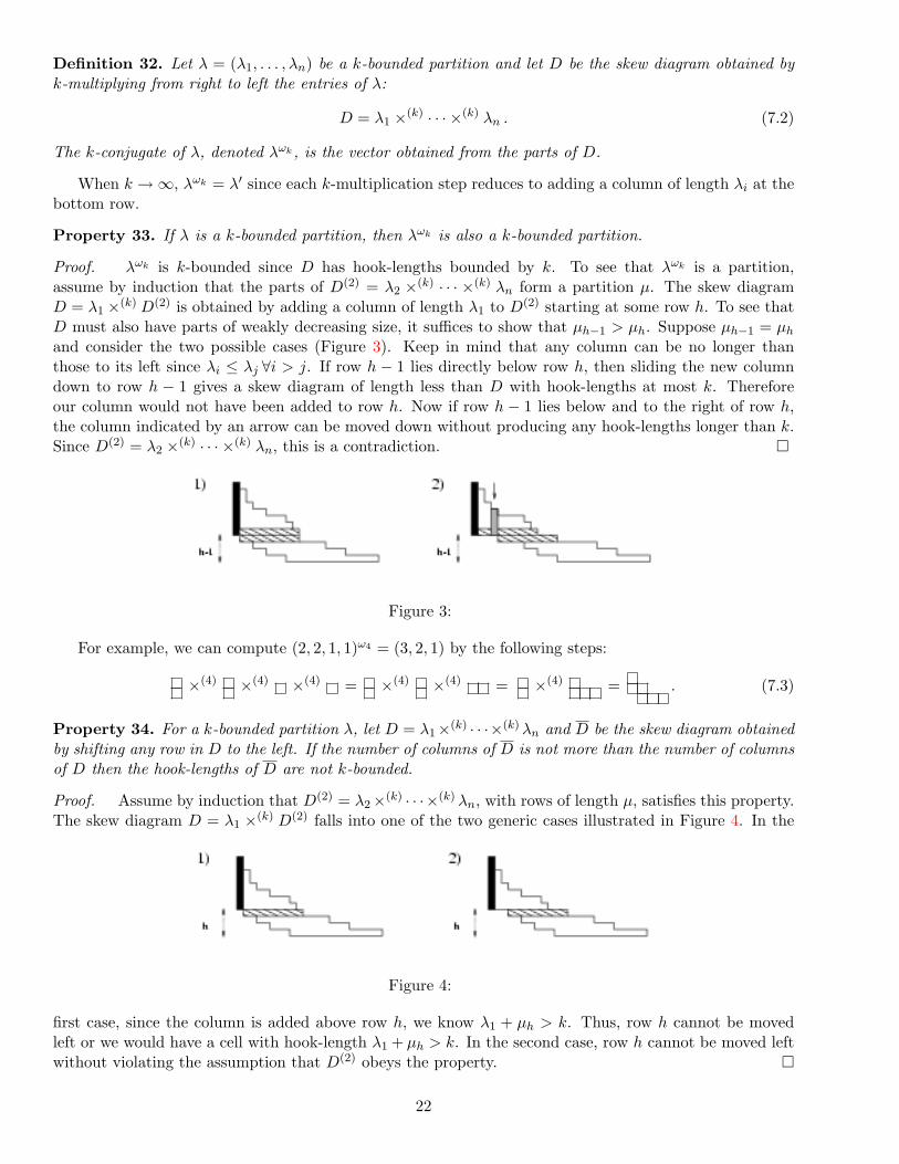
Property 33. If λ is a k-bounded partition, then λωk is also a k-bounded partition.

Proof. λωk is k-bounded since D has hook-lengths bounded by k. To see that λωk is a partition,assume by induction that the parts of D(2) = λ2 ×(k) · · · ×(k) λn form a partition µ. The skew diagramD = λ1 ×(k) D(2) is obtained by adding a column of length λ1 to D(2) starting at some row h. To see thatD must also have parts of weakly decreasing size, it suffices to show that µh−1 > µh. Suppose µh−1 = µh

and consider the two possible cases (Figure 3). Keep in mind that any column can be no longer thanthose to its left since λi ≤ λj ∀i > j. If row h − 1 lies directly below row h, then sliding the new columndown to row h − 1 gives a skew diagram of length less than D with hook-lengths at most k. Thereforeour column would not have been added to row h. Now if row h − 1 lies below and to the right of row h,the column indicated by an arrow can be moved down without producing any hook-lengths longer than k.Since D(2) = λ2 ×(k) · · · ×(k) λn, this is a contradiction. �

Figure 3:

For example, we can compute (2, 2, 1, 1)ω4 = (3, 2, 1) by the following steps:

×(4) ×(4) ×(4) = ×(4) ×(4) = ×(4) = . (7.3)

Property 34. For a k-bounded partition λ, let D = λ1×(k) · · ·×(k) λn and D be the skew diagram obtainedby shifting any row in D to the left. If the number of columns of D is not more than the number of columnsof D then the hook-lengths of D are not k-bounded.

Proof. Assume by induction that D(2) = λ2×(k) · · ·×(k) λn, with rows of length µ, satisfies this property.The skew diagram D = λ1 ×(k) D(2) falls into one of the two generic cases illustrated in Figure 4. In the

Figure 4:

first case, since the column is added above row h, we know λ1 + µh > k. Thus, row h cannot be movedleft or we would have a cell with hook-length λ1 + µh > k. In the second case, row h cannot be moved leftwithout violating the assumption that D(2) obeys the property. �

22

Theorem 35. ωk is an involution on partitions bounded by k. That is, for λ with λ1 ≤ k,

(λωk)ωk = λ . (7.4)

Proof. Let D = λ1 ×(k) · · · ×(k) λn. Property 34 implies that D is recovered by performing the k-multiplication of the entries of λωk in a conjugate way (adding rows to the leftmost position such thatthe hook-lengths are never larger than k). Therefore, if λωk = µ, the conjugate of D is given by D′ =µ1 ×(k) · · · ×(k) µm, and thus (D′)′ = D implies that µωk = (λωk)ωk = λ. �

Given the k-conjugation of a partition, it is natural to consider the relation among an atom indexed byλ and the atom indexed by λωk . In fact, our examples suggest that conjugating each tableaux in an atomproduces the tableaux in another atom.

Conjecture 36. Let T be a standard tableau. For any copy A(k)T of A(k)

λ ,(A(k)

T

)t = A(k)T ′ , (7.5)

for some standard tableau T ′ of shape λωk .

Since, at any level, there is at least one copy of each atom of a given degree in the set of standardtableaux, we have the following corollary:

Corollary 37. In any atom of shape λ and level k, there is a unique element of maximal charge whoseshape is the conjugate of λωk , (λωk)′.

Furthermore, since a standard tableau T in n letters satisfies charge(T t)=(n2

)−charge(T ),

Corollary 38. Let ω be the involution such that ωSλ[X] = Sλ′ [X]. Then, for some ∗ ∈ N,

ω A(k)λ [X; t] = t∗A

(k)λωk [X; 1/t] . (7.6)

Here we see that for large k, λωk = λ′ is consistent with the fact that A(k)λ [X; t] = Sλ[X] in this case.

8 Pieri rules

Beautiful combinatorial algorithms are known for the Littlewood-Richardson coefficients that appear in aproduct of Schur functions;

Sλ Sµ =∑ν

cνλµ Sν . (8.1)

Recall by Property 6 that our atoms A(k)λ [X; t] are simply the Schur functions Sλ when k is large. Therefore

the expansion coefficients in a product of atoms are the Littlewood-Richardson coefficients when k is largeand it is natural to examine the coefficients in a product of two atoms for general k. In fact, in the caset = 1, the coefficients in a product of two atoms do seem to generalize Littlewood-Richardson coefficients.

Conjecture 39. Let A(k)λ denote the case t = 1 in A

(k)λ [X; t]. Then

A(k)λ A(k)

µ =∑ν

cνλµ

(k)A(k)ν , where 0 ⊆ cν

λµ(k) ⊆ cν

λµ . (8.2)

In particular, we knowcνλµ

(k) = cνλµ for k ≥ |µ| . (8.3)

Identity 8.1 reduces to the Pieri rule when λ is a row (resp. column). Since an atom A(k)λ reduces to h`

(resp. e`) when λ is a row (column) of length ` ≤ k, our conjecture can be reduced to a k-generalizationof the Pieri rule.

23

Corollary 40. For given sets of tableaux E(k)λ,` and E

(k)λ,` , we have for ` ≤ k,

h` A(k)λ =

∑µ∈E

(k)λ,`

A(k)µ and e` A

(k)λ =

∑µ∈E

(k)λ,`

A(k)µ . (8.4)

We believe the sets E(k)λ,` and E

(k)λ,` are defined in a manner analogous to the Pieri rule.

Conjecture 41. For any positive integer ` ≤ k,

E(k)λ,` = {µ |µ/λ is a horizontal `-strip and µωk/λωk is a vertical `-strip} ,

E(k)λ,` = {µ |µ/λ is a vertical `-strip and µωk/λωk is a horizontal `-strip} . (8.5)

For example, to obtain the indices of the elements that occur in e2 A(4)3,2,1, we compute (3, 2, 1)ω4 =

(2, 2, 1, 1) by Definition 32 and then add a horizontal 2-strip to (2,2,1,1) in all possible ways. This gives(2,2,2,1,1),(3,2,1,1,1),(3,2,2,1) and (4,2,1,1) of which all are 4-bounded. Our set then consists of all the4-conjugates of these partitions that leave a vertical 2-strip when (3, 2, 1) is extracted from them. Thecorresponding 4-conjugates are

(2, 2, 2, 1, 1)ω4 = , (3, 2, 1, 1, 1)ω4 = , (3, 2, 2, 1)ω4 = , (4, 2, 1, 1)ω4 = , (8.6)

and of these partitions, only the first three are such that a vertical 2-strip remains when (3, 2, 1) is extracted.Therefore

e2 A(4)3,2,1 = A

(4)3,3,2 + A

(4)3,2,2,1 + A

(4)3,2,1,1,1 . (8.7)

9 Hook case

We are able to explicitly determine the functions A(k)λ [X; t] in the case that λ is a hook partition and also

to derive properties of atoms indexed by partitions slightly more general then hooks. These results rely onthe following property of a row-shaped katabolism.

Property 42. If T has shape λ = (m, 1r) (a hook), then

K(n) : T −→{

T if n ≤ m

0 otherwise, (9.1)

where T is also hook-shaped.

Proof. Consider a tableau T of shape λ = (m, 1r). If n > m then T does not contain a row of length nand thus K(n)T = 0. Assume n ≤ m. Let U be the tableau of shape (1r) obtained by deleting the bottomrow of T . By the definition of katabolism, the action of K(n) on T amounts to row inserting a sequence ofstrictly decreasing letters (those of U) into a sequence of weakly increasing letters (the last m − n lettersin the bottom row of T ). The insertion algorithm implies [1] that in this case, no two elements may beadded to the same row and therefore, we obtain a hook shape. �

This property leads to the hook content of any atom that is not indexed by a k-generalized hookpartition, that is, a partition of the form (k, . . . , k, ρ1, ρ2, . . .) for a hook shape (ρ1, ρ2, . . .).

Property 43. If T is a tableau of shape λ, where λ is not a k-generalized hook, then A(k)T does not contain

any tableaux with a hook shape.

24

Corollary 44. If λ is a partition that is not a k-generalized hook, then

A(k)λ [X; t] = Sλ[X] +

∑µ>λ

v(k)µλ (t) Sµ[X] , (9.2)

where v(k)µλ (t) = 0 for all hook partitions µ.

Proof. Let λ→k = (λ(1), λ(2), . . .). The condition on λ implies that λ2 is at least 2. If we first considersuch partitions with λ1 6= k then λ(1) cannot be a hook (λ1 6= k implies that the first partition in the k-splitcontains at least the first two parts of λ). But if λ(1) is not a hook, then any hook-shaped tableau T inB(λ1)

(A(k)

(λ2,λ3,... )

)will not contain the shape λ(1) and will therefore be sent to zero under Pλ→k . On the

other hand, if λ1 = k then λ(1) = (k). Now any hook-shaped tableau T in B(λ1)

(A(k)

(λ2,λ3,... )

)will be sent

to a hook under the (k)-katabolism by Property 42. Our claim thus follows recursively on the remainingterms of the k-split of λ. �

If an atom is indexed by a k-generalized hook, we can determine it explicitly.

Property 45. Let λ = (m, 1r) be a k-irreducible hook partition. Then

A(k)λ =

{(r + 1) r · · · 2 1m if r + m ≤ k

(r + 1) r · · · 2 1m + r · · · 2 1m (r + 1) otherwise. (9.3)

Note, here an element (r + 1) r · · · 2 1m denotes the word (r + 1) r · · · 2 1 1 · · · 1.

Proof. Since r, m ≤ k − 1 in any k-irreducible partition λ = (m, 1r), we have that (1i)→k = (1i) for1 ≤ i ≤ r. Therefore, on a tableau T with i boxes, P(1i)→kT 6= 0 only for T of shape (1i) and thus

A1r = P(1r)→k B1 · · ·P(12)→k B1P(1)→k B1 H0 = r r − 1 · · · 1 . (9.4)

Moreover, it develops that Bm A1r = (r + 1) r · · · 2 1m + r · · · 2 1m (r + 1). Now we have

A(m,1r) = P(m,1r)→k

((r + 1) r · · · 2 1m + r · · · 2 1m (r + 1)

). (9.5)

Since r + m− k ≤ k, the k-split of (m, 1r) is

(m, 1r)→k =

{((m, 1r)

)if r + m ≤ k(

(m, 1k−m), (1r+m−k))

otherwise. (9.6)

In either case, P(m,1r)→k ((r + 1) r · · · 2 1m) = (r + 1) r · · · 2 1m, but since r · · · 2 1m (r + 1) never containsshape (m, 1r), P(m,1r)→k (r · · · 2 1m (r + 1)) 6= 0 only in the second case. �

Now by Conjecture 21, we use the given atoms of level k indexed by a k-irreducible hook shape toobtain more general cases including those indexed by a k-generalized hook shape.

Corollary 46. For a sequence of k-rectangles (R1, R2, . . . , Rj), let λ the partition rearrangement of(R1, R2, . . . , Rj ,m, 1r). Then

A(k)λ [X; t] ∝ z

(BR1 · · ·BRj A(m,1r)

). (9.7)

References

[1] W. Fulton, Young Tableaux: with Applications to Representation Theory and Geometry, CambridgeUniversity Press, 1997.

[2] A. M. Garsia and M. Haiman, A graded representation module for Macdonald’s polynomials, Proc.Natl. Acad. Sci. USA 90 (1993) 3607-3610.

25

[3] M. Haiman, Hilbert schemes and Macdonald polynomials: the Macdonald positivity conjecture,http://www.math.ucsd.edu/˜mhaiman/.

[4] D.E. Knuth, Permutations, matrices and generalized Young tableaux, Pacific J. Math 34 (1970), 709–727.

[5] L. Lapointe and J. Morse, Tableaux statistics for two part Macdonald polynomials, math.CO/9812001.

[6] A. Lascoux, B. Leclerc and J.-Y. Thibon, Ribbon tableaux, Hall-Littlewood functions, quantum affinealgebras and unipotent varieties, J. Math. Phys. 38 (1997), 1041–1068.

[7] A. Lascoux, B. Leclerc and J.-Y. Thibon, The Plactic Monoid, in Combinatorics on Words, M.Lothaire, Academic Press (to appear), http://www-igm.univ-mlv.fr/˜jyt/.

[8] A. Lascoux and M.-P. Schutzenberger, Sur une conjecture de H.O. Foulkes, C.R. Acad. Sc. Paris. 294(1978), 323–324.

[9] A. Lascoux and M.-P. Schutzenberger, Le monoıde plaxique, Quaderni della Ricerca scientifica 109(1981), 129–156.

[10] I. G. Macdonald, Symmetric functions and Hall polynomials, 2nd edition, Clarendon Press, Oxford,1995.

[11] G. de B. Robinson, On the representations of the symmetric group, Amer. J. Math. 60, (1938), 745–760.

[12] C. Schensted, Longest increasing and decreasing subsequences, Canad. J. Math. 13 (1961), 179–191.

[13] A. Schilling and S. Warnaar, Inhomogeneous lattice paths, generalized Kostka-Foulkes polynomials,and An−1-supernomials, math.QA/9802111.

[14] M. Shimozono, A cyclage poset structure for Littlewood-Richardson tableaux, math.QA/9804037.

[15] M. Shimozono and J. Weyman, Graded characters of modules supported in the closure of a nilpotentconjugacy class, math.QA/9804036.

[16] M. Shimozono and M. Zabrocki, Hall-Littlewood vertex operators and generalized Kostka polynomials,math.QA/0001168.

[17] S. Veigneau, ACE, an Algebraic Combinatorics Environment for the computer algebra system MAPLE ,Version 3.0 ,1998, http://phalanstere.univ-mlv.fr/˜ace/.

[18] M.A. Zabrocki, A Macdonald vertex operator and standard tableaux statistics for the two-column (q,t)-Kostka coefficients, Electron. J. Combinat. 5, R45 (1998).

26

......................................

........................................................................................................

........................................................................................................

........................................................................................................

........................................................................................................

........................................................................................................

........................................................................................................

...................................... ...........................

...........

..................................................................................................................................

..................................................................................................................................

.......................................................................................................................................................................................................................................................

...................................... ...........................

...........

..................................................................................................................................

......................................

..............................................................................................................................................................................................................................

......................................

........................................................................................................

........................................................................................................

........................................................................................................

........................................................................................................

........................................................................................................

........................................................................................................

......................................

..................................................................................................................................

........................................................................................................

........................................................................................................

........................................................................................................

........................................................................................................

........................................................................................................

........................................................................................................

........................................................................................................

........................................................................................................

........................................................................................................

........................................................................................................

A(4)1

A(4)0

A(4)1,1

A(4)3

A(4)3,1,1A

(4)3,2

A(4)3,2,1

A(4)3,2,2

A(4)2

A(4)1,1,1

A(4)3,1 A

(4)2,1,1

A(4)2,2,1 A

(4)2,1,1,1

A(4)2,2,1,1

A(4)2,2,1,1,1

A(4)3,2,2,1 A

(4)3,2,1,1,1

A(4)2,1

A(4)2,2

A(4)3,1,1,1

A(4)3,2,1,1

A(4)3,2,2,1,1

A(4)3,2,2,1,1,1

......................................

........................................................................................................

........................................................................................................

........................................................................................................

........................................................................................................

......................................

A(4)2

A(3)0

A(3)1

A(3)1,1

A(3)2,1

A(3)2,1,1

Figure 5: Action of e1 on irreducible atoms of level 3 and 4

27

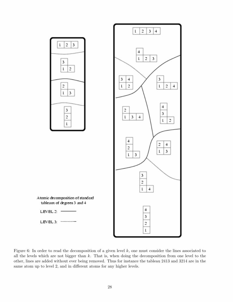
Figure 6: In order to read the decomposition of a given level k, one must consider the lines associated toall the levels which are not bigger than k. That is, when doing the decomposition from one level to theother, lines are added without ever being removed. Thus for instance the tableau 2413 and 3214 are in thesame atom up to level 2, and in different atoms for any higher levels.

28

Figure 7: See Figure 6 for details on how to read the figure.

29