http://curve.coventry.ac.uk/open

A Low Collision and High Throughput Data Collection Mechanism for Large-Scale Super Dense Wireless Sensor Networks Lei, C. , Bie, H. , Fang, G. , Gaura, E. , Brusey, J. , Zhang, X. and Dutkiewicz, E. Published PDF deposited in Curve September 2016 Original citation: Lei, C. , Bie, H. , Fang, G. , Gaura, E. , Brusey, J. , Zhang, X. and Dutkiewicz, E. (2016) A Low Collision and High Throughput Data Collection Mechanism for Large-Scale Super Dense Wireless Sensor Networks. Sensors, volume 16 (7): 1108 URL: http://dx.doi.org/10.3390/s16071108 DOI: 10.3390/s16071108 Publisher: MDPI This is an open access article distributed under the Creative Commons Attribution License (CC BY 4.0) Copyright © and Moral Rights are retained by the author(s) and/ or other copyright owners. A copy can be downloaded for personal non-commercial research or study, without prior permission or charge. This item cannot be reproduced or quoted extensively from without first obtaining permission in writing from the copyright holder(s). The content must not be changed in any way or sold commercially in any format or medium without the formal permission of the copyright holders.

CURVE is the Institutional Repository for Coventry University

sensors

Article

A Low Collision and High Throughput DataCollection Mechanism for Large-Scale SuperDense Wireless Sensor NetworksChunyang Lei 1, Hongxia Bie 1,*, Gengfa Fang 2, Elena Gaura 3, James Brusey 3, Xuekun Zhang 1

and Eryk Dutkiewicz 2

1 School of Information and Communication Engineering, Beijing University of Posts and Telecommunications,Beijing 100876, China; leichunyang.2014@gmail.com (C.L.); zhangxuekun1990@gmail.com (X.Z.)

2 School of Computing and Communications, University of Technology Sydney, Sydney 2109, Australia;gengfa.fang@uts.edu.au (G.F.); Eryk.Dutkiewicz@uts.edu.au (E.D.)

3 Faculty of Engineering and Computing, Coventry University, Coventry CV1 5FB, UK;e.gaura@coventry.ac.uk (E.G.); james.brusey@gmail.com (J.B.)

* Correspondence: biehx@bupt.edu.cn; Tel.: +86-138-1048-9874

Academic Editor: Leonhard M. ReindlReceived: 15 June 2016; Accepted: 11 July 2016; Published: 18 July 2016

Abstract: Super dense wireless sensor networks (WSNs) have become popular with the developmentof Internet of Things (IoT), Machine-to-Machine (M2M) communications and Vehicular-to-Vehicular(V2V) networks. While highly-dense wireless networks provide efficient and sustainable solutionsto collect precise environmental information, a new channel access scheme is needed to solve thechannel collision problem caused by the large number of competing nodes accessing the channelsimultaneously. In this paper, we propose a space-time random access method based on a directionaldata transmission strategy, by which collisions in the wireless channel are significantly decreased andchannel utility efficiency is greatly enhanced. Simulation results show that our proposed methodcan decrease the packet loss rate to less than 2% in large scale WSNs and in comparison with otherchannel access schemes for WSNs, the average network throughput can be doubled.

Keywords: medium access control; carrier sensing range; data collection; wireless sensor network

1. Introduction

Wireless sensor networks (WSNs) play an important role in sensing and collecting a wide rangeof environmental and geological parameters in the current and future surveillance systems. In suchnetworks, widely covered and densely deployed sensors may simultaneously detect the sensing dataand they need to send the data to a sink node. As a result, the effective network throughput willbe severely decreased because of the collisions among the contending sensors accessing the wirelesschannel simultaneously. With the increasing demand for high network converge and sensor densitywith new applications such as Internet of Things (IoT) and Vehicular-to-Vehicular (V2V) networks, thepossibility of collisions among WSN nodes has become too high for WSNs to work well. Therefore,how to achieve effective data collection through an efficient channel access and scheduling mechanismso as to decrease the collisions becomes a new challenge in the new IoT and V2V types of superdense WSNs.

In Carrier Sense Multiple Access with Collision Avoidance (CSMA/CA) based networks, thetransmission by hidden nodes causes severe interference, i.e., collision, to an on-going transmission inWSNs. In this paper, we focus on seeking a new method to avoid such interference.

So far, channel estimation based backoff algorithms [1,2] have been proposed to avoid collisionsamong the neighbor nodes. In such algorithms, nodes adaptively schedule their time to access the

Sensors 2016, 16, 1108; doi:10.3390/s16071108 www.mdpi.com/journal/sensors

Sensors 2016, 16, 1108 2 of 16

channel by continuously estimating the contention levels among their neighbor nodes. It has beenshown in [3] that channel estimation based backoff algorithms can efficiently decrease collisions amongneighbor nodes to the theoretical low bound in cases with a wide range of contention levels. However,such algorithms are invalid for the case of collisions from hidden nodes because collisions from hiddennodes are too complex and hard to monitor on-the-fly.

Decreasing the possibility of collisions from hidden nodes with as small throughput loss aspossible is challenging. In recent years, the studies in [4–6] re-evaluated the Channel Clear Assessment(CCA) function and tried to solve the hidden terminal problem by proposing new solutions based onthe new concept of efficient Carrier Sense Ranges (CSR). By enabling the non-hidden nodes to detectand hear the hidden nodes’ activities, the hidden nodes will no longer be hidden for others. Thus, a lotof interference analysis models have been proposed since then for better CSRs for different applications.The authors in [7–10] proposed Protocol Interference Models (PrIMs) to improve performance of CSRsin networks with diverse topologies. In their models, the interference introduced by a hidden node toan on-going communication is comprehensively analyzed, and a “safe” CSR is calculated to preventthe on-going communication from being corrupted by this hidden node. However, the work in [4]indicated that PrIMs is idealistic because the interference in reality is not from a single hidden nodebut from multiple hidden nodes. As a consequence, the CSRs calculated from PrIMs are not largeenough to effectively avoid collisions caused by hidden nodes. A new interference analysis model,Physical Interference Model (PhIM), was proposed in [11,12]. In these papers, interferences from allpossible hidden terminals are included so that the CSRs calculated from PhIMs can totally avoid thecollisions from hidden nodes even in the worst case. However, in practice, interference from hiddennodes is not always that serious. This suggests that the estimated CSRs in PhIMs sometimes becomelarger than the correct value of CSR. An over-estimated CSR will cause the explosion problem andsome contending nodes will miss the transmission opportunities. As a result, the effective channelutilization rate, which has a positive correlation with the system throughput, will be decreased.

In this paper, we propose an effective method to improve the network throughput performanceby controlling the interference from neighbor nodes including hidden nodes. Our main contributionsin this paper are summarized as bellow:

Firstly, we analyze the characteristics of the pre-configuring operations in WSNs. Based on suchoperations, we propose a data collection scheme with distinct directivity. We validate of this directionaltransmission scheme on the premise of complete data collection.

Secondly, we analyze collisions in WSNs and propose a space-time based medium accessmechanism, which explores user diversity both in space and time domains. By fully taking advantageof the directional transmission strategy, we propose a new method of calculatingCSRs for the proposedchannel access mechanism to significantly reduce or even totally eliminate in some cases collisionsfrom both neighbor nodes and hidden nodes.

Thirdly, we conduct simulations to evaluate the performance of our proposed solution, which wascompared to the classic IEEE 802.11 series protocols and ones with enhanced CSRs. We analyze thethroughput and the packet loss rate, the key parameters that determine the data collection efficiency. Inorder to cover scenarios with different settings, we evaluate the performance of our proposed solutionin networks with different topologies, including the regular latticed case and random deployed ones.

This paper is organized as follows. In Section 2 we analyze the channel access characteristics inWSNs and propose a new directional data transmission strategy. A space-time based random accessmethod is proposed in Section 3. In Section 4, we evaluate the performance of the proposed methodthrough simulations. In Section 5 we conclude this paper.

2. Data Collection Strategy with Directional Transmission

Communications in WSNs are quite different from general wireless networks in that the dataflow is quite directional, i.e., either from the sink node to end nodes or vice versa. In this section,

Sensors 2016, 16, 1108 3 of 16

we analyze these properties ofa WSNs and propose our new data collection strategy with directionaltransmission characteristics.

2.1. Pre-Configuring Operation in WSNs

In WSNs, a sink node is the controller of the whole network by sending commands to othersensors, including monitoring the sensors’ status, broadcasting commands to sensors, etc. This taskis called the run-up phase. The second task for WSNs is to collect data from all the sensors wheredata will be sent to the sink node using intermediate relay sensor nodes. This task is called thedata-collection phase. Controlled by the sink node, the WSN can either be in the run-up phase ordata-collection phase.

The run-up phase of the WSN happens during the network deployment process when somesimple interactions happen between the sensors and the sink node. For example, the sink node willunicast, multicast or broadcast commands to sensors and then the sensors will report their stateinformation back to the sink node, i.e., their position, battery, routing information, etc. to the sink node.By checking the information above, the sink node can ensure the network connectivity while sensorscan update their information to the sink node.

The data-collection phase happens when an event is detected by sensors so that the sensors needto send data back to the sink node. During this period of time, a large number of nearby sensors willsimultaneously attempt to get access to the channel in order to transmit the data to the sink node.Since CSMA/CA is not good at supporting large users contending for channel access, the above casewill result in serious collisions among the sensors which significantly decreases network throughputand introduce more delay.

Considering those characteristics of communications in WSNs, it is necessary to introducecentralized control, i.e., making some pre-configurations to sensors and introducing some rulesto define specific behaviours of sensors especially during the run-up phase. With the pre-configurationin the run-up phase, data transmissions in the data-collection phase can be well controlled by avoidingextreme congestions, so that collisions are able to be suppressed.

2.2. Directional Transmission Model

Directional data forwarding is a typical feature of communications in WSNs because the data flowin WSNs is always directional, i.e., it is either from sensors to the sink node or vice versa. Consideringthe pre-configuring operations during the run-up phase, the property of directional data transmissionsin WSNs can be further utilized and the interference among nodes can be better mitigated. Next,we focus on the analysis of the directional transmission model.

We start with the physical model of a sensor network. As shown in Figure 1, we consider a sensornetwork which includes n wireless sensor nodeV = {v1,v2, · · ·,vn } and a sink node s. We use a randomextended network model [13] by assuming that sensor nodes are uniformly deployed in a rectangularregion with the size of a ×b.

We denote the location of the sensor node vt in the network by

vtde f

(xt ,yt ) (1)

where xt and yt represent the location coordinates. We denote the distance between vt and vr as theeuclidean space | |vt −vr | | and the communication range as R, which is associated with the Signal toInterference plus Noise Ratio (SINR). If | |vt −vr | | ≤ R, data transmission fromvt tovr will be successful.We denote the link as l (vt ,vr ) and express the links in the network as Equation (2).

L = {l (vt ,vr ) | | |vt −vr | | ≤ R,vt ,vr ∈ V } (2)

Sensors 2016, 16, 1108 4 of 16

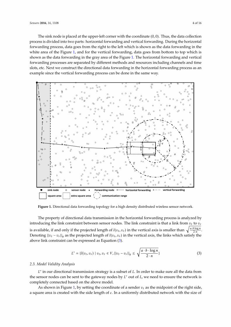
The sink node is placed at the upper-left corner with the coordinate (0, 0). Thus, the data collectionprocess is divided into two parts: horizontal forwarding and vertical forwarding. During the horizontalforwarding process, data goes from the right to the left which is shown as the data forwarding in thewhite area of the Figure 1, and for the vertical forwarding, data goes from bottom to top which isshown as the data forwarding in the gray area of the Figure 1. The horizontal forwarding and verticalforwarding processes are separated by different methods and resources including channels and timeslots, etc. Next we construct the directional data forwarding in the horizontal forwarding process as anexample since the vertical forwarding process can be done in the same way.

𝟓

𝟐𝒄

R

𝐜

square area extra square area

horizontal forwarding vertical forwardingsink node sensor node Forwarding node

communication range

Figure 1. Directional data forwarding topology for a high density distributed wireless sensor network.

The property of directional data transmission in the horizontal forwarding process is analyzed byintroducing the link constraint between sensor nodes. The link constraint is that a link from vt to vr

is available, if and only if the projected length of l (vt ,vr ) in the vertical axis is smaller than√

a ·b logn2·n .

Denoting | |vt −vr | |y as the projected length of l (vt ,vr ) in the vertical axis, the links which satisfy theabove link constraint can be expressed as Equation (3).

L∗ = {l (vt ,vr ) | vt ,vr ∈ V , | |vt −vr | |y ≤

√a · b · logn

2 · n} (3)

2.3. Model Validity Analysis

L∗ in our directional transmission strategy is a subset of L. In order to make sure all the data fromthe sensor nodes can be sent to the gateway nodes by L∗ out of L, we need to ensure the network iscompletely connected based on the above model.

As shown in Figure 1, by setting the coordinate of a sender vt as the midpoint of the right side,a square area is created with the side length of c. In a uniformly distributed network with the size of

Sensors 2016, 16, 1108 5 of 16

a ×b, the probability of a random deployed sensor node within the above square area is equal to c2

a ·b .Thus, in a n-node system, the probability of having an empty square area can be calculated by

pn = (1 −c2

a · b)n (4)

where

c =

√2 · a · b · lnn

n(5)

Because 1 − x ≤ exp(−x ), we have

pn ≤ exp(−n · c2

a · b) =

1n2 (6)

and∞∑n=1

pn < ∞ (7)

According to the Borel-Cantelli lemma, there is at least one sensor node located in the square areafor sufficiently large n.

As shown in Figure 1, if the communication range R is larger than√

52 · c, at least one sensor node

can be selected as a receiver by the sender vt to establish a link. Because vt is in the middle of the rightside of the square, the projected length of the link in the vertical axis is smaller than c

2 . Forwarding datafrom all the sensor nodes to the gateway nodes through the links in set L∗ is feasible. As the numberof sensor nodes located in the square area is a binomial random variable with parameters ( c2

a ·b ,n),the availability of links in the square area is guaranteed. As shown in Figure 1, if the communicationrange R is large enough, which is very common in practice, the sender vt can select receivers fromother nearby square areas. In this situation, more links to do the data forwarding are available.

Now, we define ρ = na×b , where ρ represents the sensor density of a WSN. According to

Equation (5), a smaller square area can be constructed by larger ρ. In a dense WSN, our proposeddirectional data forwarding scheme for both the horizontal and vertical cases can be modelled asa problem of bunch of parallel-arranged lines with certain offsets which decrease significantly as afunction of the sensor nodes density. For the scenarios that a WSN has a regular latticed topology, thedata forwarding links are in parallel to each other with no offsets and can be expressed as c = 0.

3. A Space-Time Based Random Access Mechanism

3.1. Collisions Analysis

The set of nodes that have collisions with the data transmission from vt to vr can be defined asconcurrent nodes. Because there are multiple concurrent nodes, the concurrent nodes can be furthergrouped as concurrent senders, which are the nodes that are sending data to their correspondingreceivers and concurrent receivers that are passively responding to the corresponding senders forhandshaking purpose.

Base on the literature review on the Carrier Sense Range (CSR), the proposed CSR based schemesto protect the on-going transmission from being collided by concurrent nodes, can be expressedas follows:

CSR = (K + β ) · dmax (8)

where dmax is the maximum link length in the network. K is a coefficient calculated from thesignal propagation loss model [4,11]. All the concurrent nodes including both concurrent sendersand receivers are considered in the model above. The power levels of those concurrent nodes areaccumulated at the receiver as interference and K is determined to make sure that the lower bound ofthe signal to interference plus noise ratio (SINR) at the receiver is larger than a given threshold.

Sensors 2016, 16, 1108 6 of 16

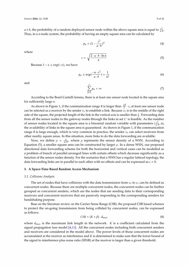
K · dmax defines the range which eliminates collisions from concurrent nodes. However, it doesnot differentiate the roles of the concurrent nodes involved, if they are the concurrent senders orreceivers, or their position information. In order to make a receiving node maintain an ideal SINRaccording to K · dmax , an extra range is needed to better separate the transmissions between concurrentnodes as sources of interference and the receiver of interest. The above problem through the two pairsof communications (T1,R2) and (T2,R2) is illustrated in Figure 2. The carrier sense range is initiallydefined by K · dmax . As shown in Figure 2a, T1 and T2 are out of each other’s carrier sensing range.As a result, the sending activity of T2 can not be stopped by the sending node T1. However, the noisefrom T2 may collide with R1’s received signal. This problem can be solved through extending CSR

by dmax as shown in Figure 2b. R1’s signal may also collide with the signal between T2 and R2 inFigure 2c because of the directional communication introduced. In this case, CSR needs to be extendedby another dmax to eliminate the collisions as shown in Figure 2d. An extra extension of CSR is definedas β . According to the existing literature, the value of β is often larger than 2.

𝑅1

𝑇1 𝑅1 𝑇2 𝑅2

𝑇1 𝑅1 𝑇2𝑅2

𝑇1 𝑅2

𝑇2

𝑇1 𝑅1 𝑇2𝑅2

𝐾 ∙ 𝑑𝑚𝑎𝑥

𝑑𝑚𝑎𝑥

𝑑𝑚𝑎𝑥𝑑𝑚𝑎𝑥

𝐾 ∙ 𝑑𝑚𝑎𝑥

𝑇2

𝑑𝑚𝑎𝑥

(𝒂)

(𝒃)

(𝒄)

(𝒅)

Figure 2. Diagram of interference from concurrent senders on the basis of coefficient K .

According to the above analysis, the network topology, the positions of the concurrent sendersand receivers, and the data transmission direction can jointly determine the value of the carrier senserange. With the directional transmission strategy, the positions of the concurrent nodes and thedata transmission directions can be well controlled to minimize collisions. A new random mediumaccess scheme is further proposed to allow multiple users to access the channel from both space andtime domains.

3.2. Space-Time Based Random Access Mechanism

We define the coordinate system as follows. The data forwarding direction is denoted as thex-axis, and then the sensor nodes are grouped as B-group along the x-axis according to Equation (9).

Bi = {vt | xt ∈ [i ·D, i ·D +D)}, i = 0, 1, 2, · · · (9)

where D is the width of B-group. Based on the grouping rules in Equation (9), the sensor nodes aredivided into ∆ groups, which are named as the G-group according to Equation (10):

Gk =⋃i=0

Bi ·∆+k ,k = 0, 1, · · ·,∆ − 1 (10)

Sensors 2016, 16, 1108 7 of 16

The data collection time is divided into Ts and sensor nodes in Gk can only access the channelduring the time interval of Tk .

Tk =⋃i=1

[i · ∆ − k − 1, i · ∆ − k ) ·T (11)

3.3. CSR for Space-Time Based Random Access Mechanism

According to the system model above, concurrent senders can only exist in the same G-groupbased on the fact that only the nodes belonging to the same G-group can access the channel at thesame time interval of T . The concurrent senders are divided into two categories based on whetherthey belong to the same B-group or not. Next, the CSRs are designed for our proposed random accessmechanism to eliminate collisions and its performance is evaluated.

3.3.1. Eliminating Interference from the Same B-Group

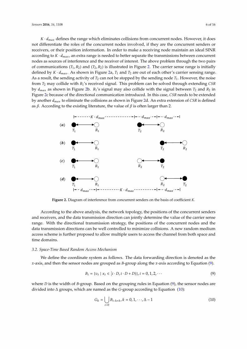
The interference from concurrent senders in the same B-group is analyzed through Figure 3. In thefigure, node vt with coordinate (xt ,yt ) is sending data to node vr with coordinate (xr ,yr ). The carriersense range is firstly initialized into K · dmax , and the carrier sense areas of vt and vr are expressed astwo circles shaped by Equations (12) and (13).

(x − xt )2 + (y −yt )

2 = K2 · d2max (12)

(x − xr )2 + (y −yr )

2 = K2 · d2max (13)

The concurrent nodes are in a susceptible area, which contains the carrier sense area ofvr expectedfor the carrier sense area of vt . As shown in Figure 3, such a susceptible area is divided into threeparts labeled as U , V and W by the sendinд area with the width of D. We denote the left and rightboundaries of the sendinд area as L0 : x = x0 and L1 : x = x1. According to the definition of B-groupin Equation (9) and the time assignment in Equation (11), if nodes are located in a band region with thewidth of D (D = x1 − x0) access channel, the nodes in the adjacent regions are not allowed to access thechannel. Thus, the distribution of the concurrent nodes is significantly affected by the configuration ofthe sendinд area.

Figure 3. Diagram of interference from concurrent senders in the same B-group.

Sensors 2016, 16, 1108 8 of 16

Concurrent Senders Elimination

According to Figure 3, concurrent senders will only stay in the area ofU⋃V . In order to eliminate

the interference from these concurrent senders, the carrier sense area is extended to cover the areaof U

⋃V . By substituting x = x1 to Equation (13) and then working on the equation, we get the

coordinates of the two intersections A(x1,yA) and B (x1,yB ) as shown in Figure 3. From the above figure,we can get yA = yB when we have yt = yr . It can be easily proved that by setting:

CSRcs ≥√(x1 − xt )2 +max{y2

A,y2B } (14)

the concurrent senders of the transmission from vt to vr can be totally eliminated. Becausevt ∈ sendinд area, it has xt ∈ [x0,x1]. Thus, we get x1 − xt ≤ D. According to the equation of |yt −yr | ≤ c

2from the previous section, we have |yA |, |yB | ≤ K · dmax +

c2 . Based on the above, by setting:

CSRcs ≥

√D2 + (K · dmax +

c

2)2 (15)

the collisions to an on-going transmission generated by any sender in the sendinд area can be eliminated.Here, dmax is used to evaluate D and c by defining ω = D

dmaxand θ = c

dmax. Thus, Equation (15)

can be rewritten as

CSRcs ≥

√ω2 + (K +

θ

2)2 · dmax (16)

Concurrent Receivers Elimination

A sender which is out of the carrier sense range of vt is denoted as vt t (xt t ,yt t ). By defining CSR

according to Equation (16), it can have

yt t ≥ (K +θ

2) · dmax (17)

Then, vt t ’s receiver is denoted as vr r (xr r ,yr r ). According to the directional data forwardingproperty, yr r has

yr r ∈ [xr r −θ

2· dmax ,xr r +

θ

2· dmax ] (18)

By substituting Equation (17) to Equation (18), we get

yr r ≥ K · dmax (19)

Because yr r is smaller than the upper bound of the carrier sense range of vr , vr r may become theconcurrent receiver of the transmission from vt to vr . Thus as shown in Figure 3, we extend the CSR toget rid of these potential concurrent receivers according to

CSRcr ≥

√ω2 + (K + θ )2 · dmax (20)

yt t can be controlled as Equation (21) below

yt t ≥ (K + θ ) · dmax (21)

Then it hasyr r ≥ (K +

θ

2) · dmax (22)

which is out of the carrier sense range of vr .

Sensors 2016, 16, 1108 9 of 16

CSR Configuration

By comparing Equations (16) and (20) to the basic carrier sense range K · dmax , concurrent nodescan be totally eliminated if CSR is set up according to

CSR =

√ω2 + (K + θ )2 · dmax (23)

As shown in Equation (23), the safe carrier sense range is determined by three parameters K ,θ and ω. According to our analysis of the above, K is the lower bound of CSR while θ indicates themaximum data forwarding offset which is affected by the network density according to our analysis inSection 2. Thus, the only variable is ω which indicates the width of B-group D. Next, we focus on theconfiguration of D.

According to Equation (23), CSR increases as a function of D, suggesting that a larger B-groupleads to a lower channel utilization rate, which corresponds to a lower network throughput. From thispoint of view, a smaller B-group is preferred. However, the smaller B-group means that fewer nodescan be included in a single group. If B-group becomes small, some areas may become empty with nosensors, indicating that the channel utilization rate will also be decreased. This becomes worse if onlya few nodes need to transmit data and the effective channel utilization rate will decreased significantly.

In order to get a balanced size of B-group, D is set as the minimum link length in the networkdmin with the following benefits.

• Firstly, dmin is a crucial factor constrained by the network layer configuration in multi-hop datacollection networks and it can be calculated during the run-up phase.

• Secondly, a large number of short links on the data transmission path leads to a longer time ofdata forwarding. It will not only lead to channel contention but also increase the data forwardingdelay, thus dmin is always set as large as possible while considering the reliability of data reception.Thus, by setting D = dmin , B-group can contain a sufficient number of nodes sharing the channel.

• Thirdly, we set D = dmin to ensure that data will be forwarded to other B-groups during thefollowing T time slots. This structure can effectively increase the channel utility rate during a lowtraffic period.

3.3.2. Eliminating Interferences Between B-Groups

The distance between two concurrent senders belonging two different B-groups is larger than(∆ − 1) · D. According to the analysis above, there is one and only one receiver associated with thetwo senders. By denoting the maximum communication range in x-axis as dx_max , the minimumdistance between the receiver and the interfering sender is larger than (∆− 1) ·D −dx_max . According tothe conclusion in Equation (8), the safe range between a receiver and a interfering sender is larger thanK · dmax . We get

(∆ − 1) ·D −dx_max ≥ K · dmax (24)

We have dmax ≥ dx_max . By substituting it to Equation (24) and then doing some transpositions,we can get

∆ ≥(K + 1) · dmax +D

D(25)

During the groups of sensor nodes taking turns accessing the wireless channel as Equations (10)and (11) indicated, the channel utility rate will be decreased by the oversized ∆. Thus, in our proposedmethod, we can set it according to the following for any determined B-group width D.

∆ = d(K + 1) · dmax +D

De (26)

The idea of the above is to totally eliminate collisions from concurrent senders belonging todifferent B-groups.

Sensors 2016, 16, 1108 10 of 16

4. Performance Evaluation

The performance of the proposed schemes is evaluated through simulations using OMNET++ [14].The classic protocols (IEEE 802.11x [15], IEEE 802.15.4 [16]), and other channel access mechanismswith enhanced CSRs [4] are compared in this section. Simulations are conducted with differentnetwork scales. Along with the increasing of the network scales, the number of neighbor nodes andhidden nodes increase. In our simulations, the performance of different data collection strategiesis evaluated by analyzing the effects of interference from neighbor nodes and hidden nodes on thenetwork performance of throughput, collision rate and frame loss rate, which are all key factorsdetermining the data collection efficiency in WSNs. In addition, in order to cover the diversity of WSNapplications, we consider two typical topologies, i.e., the random topology and the latticed topology.

4.1. Simulation Configurations

4.1.1. PHY and MAC Layer Configurations

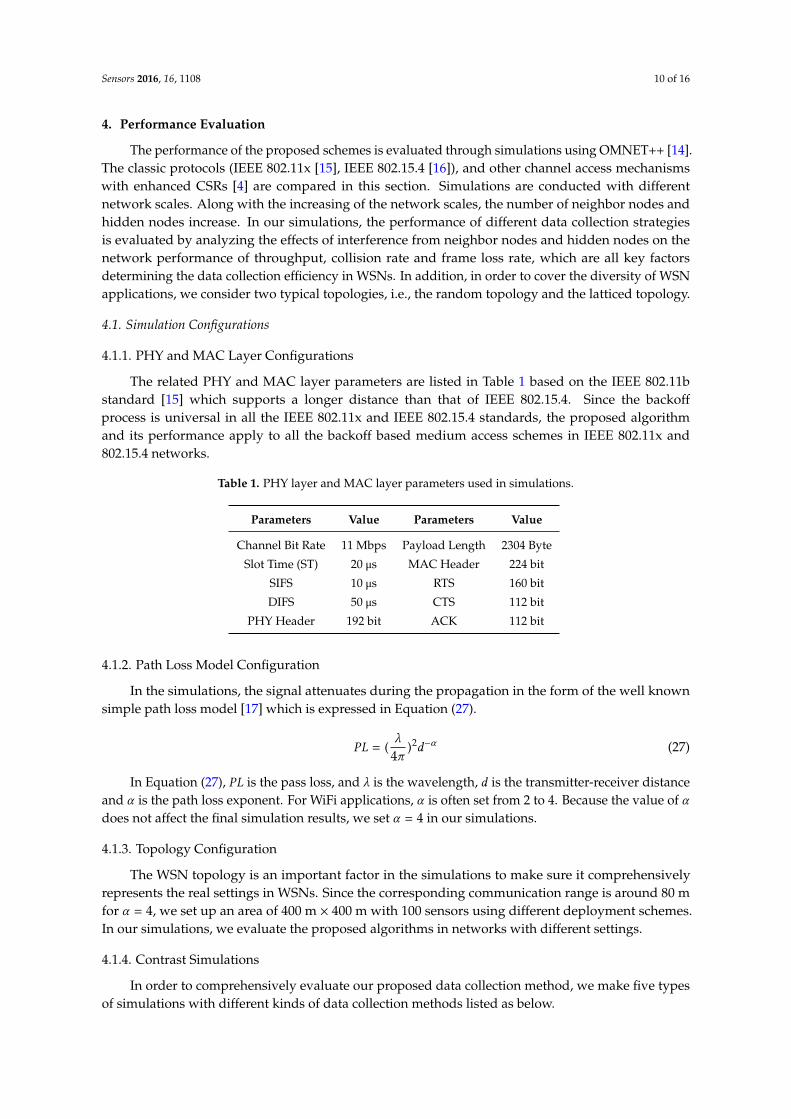
The related PHY and MAC layer parameters are listed in Table 1 based on the IEEE 802.11bstandard [15] which supports a longer distance than that of IEEE 802.15.4. Since the backoffprocess is universal in all the IEEE 802.11x and IEEE 802.15.4 standards, the proposed algorithmand its performance apply to all the backoff based medium access schemes in IEEE 802.11x and802.15.4 networks.

Table 1. PHY layer and MAC layer parameters used in simulations.

Parameters Value Parameters Value

Channel Bit Rate 11 Mbps Payload Length 2304 Byte

Slot Time (ST) 20 µs MAC Header 224 bit

SIFS 10 µs RTS 160 bit

DIFS 50 µs CTS 112 bit

PHY Header 192 bit ACK 112 bit

4.1.2. Path Loss Model Configuration

In the simulations, the signal attenuates during the propagation in the form of the well knownsimple path loss model [17] which is expressed in Equation (27).

PL = (λ

4π)2d−α (27)

In Equation (27), PL is the pass loss, and λ is the wavelength, d is the transmitter-receiver distanceand α is the path loss exponent. For WiFi applications, α is often set from 2 to 4. Because the value of αdoes not affect the final simulation results, we set α = 4 in our simulations.

4.1.3. Topology Configuration

The WSN topology is an important factor in the simulations to make sure it comprehensivelyrepresents the real settings in WSNs. Since the corresponding communication range is around 80 mfor α = 4, we set up an area of 400 m × 400 m with 100 sensors using different deployment schemes.In our simulations, we evaluate the proposed algorithms in networks with different settings.

4.1.4. Contrast Simulations

In order to comprehensively evaluate our proposed data collection method, we make five typesof simulations with different kinds of data collection methods listed as below.

Sensors 2016, 16, 1108 11 of 16

• IEEE 802.11—This is the traditional data collection method in WSNs, where all sensors areimplemented with the IEEE 802.11 protocol.

• PhIM—This is a data collection method proposed in [4] based on IEEE 802.11 with a larger CSR tototally eliminate collisions from hidden nodes and with a low signal receiving sensitivity.

• PhIM_Est—Because collisions from hidden nodes are totally eliminated in “PhIM”, the estimation-basedbackoff algorithm is used in this algorithm to further decrease collisions from neighbor nodes.Thus, this is a data collection method with the classical estimation-based backoff and idle sensealgorithm [2].

• ST -RAM—This is our proposed data collection method with updated CSRs by utilizing thedirectional data forwarding characteristics in WSNs.

• ST -RAM_Est—This is our proposed data collection method working together with theestimation-based backoff algorithm.

Next, the performance of the above five data collection methods is compared in terms ofthroughput and frame loss rate with the above two kinds of topologies.

4.2. Throughput Performance

Throughput is one of the most important performance indexes in WSNs. Figures 4 and 5 show theresults of the throughput when using different data collection methods in the networks with differentscales. The network scales ranging from 400 m × 400 m to 400 m × 3200 m are presented in the figurewhich is indicated by the x-axis. The y-axis is the average throughput of 400 m × 400 m area on average.

Figure 4. Throughput performance of different data collection methods for random deployed networkswith different scales.

Figure 4 shows the throughput as a function of the network scale with random topologies.From the figure we can see that when the network scale is small, the throughput of different datacollection methods is similar but when the network scale is increased, the throughput becomevery different.

Compared to the five different data collection methods, the throughput of “IEEE 802.11” decreasesmuch faster than of the other schemes. This is because the number of hidden nodes of an on-goingcommunication increases exponentially along with the increase of the network scale. As a result,interference from hidden nodes severely decreases the throughput of “IEEE 802.11”. The farther ahidden node is, the weaker interference it can cause. Thus, with the increase of the network scale,

Sensors 2016, 16, 1108 12 of 16

the accumulated interference from hidden nodes tends to be stable which makes the throughput of“IEEE 802.11” stable at around 5 Mbps when k is larger than 4.

Figure 5. Throughput performance of different data collection methods for lattice deployed networkswith different scales.

The throughput of “PhIM” is much higher than that of “IEEE 802.11”, because the interferencefrom hidden nodes is significantly suppressed by setting large CSR. However, with the increase ofthe network scale, the throughput of “PhIM” can only reach a certain level. It is because a largerCSR not only suppresses the number of the hidden nodes but it also increases the number of theneighbor nodes. The number of the neighbors will increase as a function of the extension of thenetwork coverage. A larger number of neighbor nodes with more serious channel contention will alsodecrease the throughput.

The throughput decrease resulting from the neighbor nodes can be relieved by “PhIM_Est” whichcan be easily verified by the two curves labeled with “PhIM” and “PhIM_Est” in the figure. It is becausethe estimation-based backoff algorithm which is applied in “PhIM_Est” can effectively reduce collisionsfrom the extremely large number of neighbor nodes.

In all the simulations, our proposed data collection method “ST -RAM” performs the best with themost stable throughput even for the cases of increasing the network scale. This is because our proposedsolution has the following three advantages: Firstly, collisions from the hidden nodes are totallyeliminated by our new proposed CSR. Secondly, the value of CSR is cut down by sufficiently utilizingthe communication rules in WSNs which significantly improves the effective channel utilization.Thirdly, sensors are allowed to access the channel in different time intervals in our proposed methodwhich further decreases collisions from neighbor nodes.

Figure 4 shows that the throughput of “ST -RAM” and that of “ST -RAM_Est” is about the same.This is reasonable because the number of concurrent neighbor nodes in our proposed methodis significantly decreased by the time division multiple access mechanism so that the number ofcontending neighbors is only around a dozen for our settings. In this case, collisions from neighbornodes are so low that the possibility of collisions that can be avoided by the estimation-based backoffalgorithms is very small. This conclusion can be verified according to the results in [3].

The throughput of different data collection methods in latticed topology is shown in Figure 5.By comparing the results in Figures 4 and 5 we can find that the throughputs of “IEEE 802.11”, “PhIM”and “PhIM_Est” in the random topology are almost the same as that of the latticed topology case.This is because the topological structure is not taken into consideration in designing the value of CSR

Sensors 2016, 16, 1108 13 of 16

by the above methods. However, in our proposed method, the position relationship among the sensorsplays an important role in obtaining better CSRs. According to Equation (23), we can find that the CSRin the latticed topology can be further optimized by substituting θ = 0 which is proved in Section 2.This conclusion is verified in Figure 5 where the throughput of “ST -RAM” and “ST -RAM_Est” in thelatticed topology are obviously higher than that in the random topology.

4.3. Collision Rate and Frame Loss Rate

Collision rate is another important performance parameter in WSNs. The MAC layer protocolof WSNs requires that if collision happens the frame will be retransmitted until it is successfullyreceived or reaches the maximum number of retransmissions tries. This retransmission mechanismis applied to avoid endless retransmissions over very bad quality links. Once the maximum numberof retransmissions is reached, the node will drop the frame. This may trigger an upper layerretransmission during which a new transmission route will be generated. However, the frame loss maybe because of the interference from other sensors. In this case, the upper layer retransmission will bealso triggered; however, this does not make any sense, because congestions in WSNs are always withina region. However, during this process, the new transmission route establishment process will cost alot of time that is tens or hundred times of an ordinary frame transmission in the MAC layer. This willcause a severe throughput decrease on the basis of the results we presented in the previous section.

Figures 6 and 7 show the results of the collision rate in using of different data collection methodsin the networks with different scales. Results shown in Figure 6 are for the case in the random topology.It can be seen that, being affected by the serious collisions from hidden nodes, “IEEE 802.11” has thehighest collision rate which is larger than 0.95 in large-scale networks. While eliminating the collisionsfrom hidden nodes and bringing a larger number of neighbor nodes, the collision rates of “PhIM” and“PhIM_Est” are close and both approach 0.6 in large-scale networks. Our proposed methods “ST -RAM”and “ST -RAM_Est” have the lowest collision rate by simultaneously decreasing the collisions fromhidden nodes and contending neighbor nodes.

1 2 3 4 5 6 7 80

0.1

0.2

0.3

0.4

0.5

0.6

0.7

0.8

0.9

1

Network Scale (k 400m400m)

Co

llis

ion

Rate

IEEE 802.11

ST-RAM

ST-RAM_Est

PhIM

PhIM_Est

FrameLoss Rate

0.865

0.125

0.015

Figure 6. The collision rate and frame loss rate of different data collection methods for randomdeployed networks with different scales.

According to the IEEE 802.11 protocol, we set the maximum number of retransmissions as 4 andsimulate the corresponding frame loss rate in networks with different scales. The approximate frameloss rates in large scale networks, where the frame loss rate becomes stable, are labeled on the rightside of Figure 6. An extremely large amount of time will be wasted on establishing a new route in

Sensors 2016, 16, 1108 14 of 16

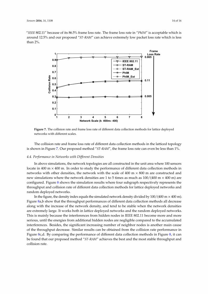
“IEEE 802.11” because of its 86.5% frame loss rate. The frame loss rate in “PhIM” is acceptable which isaround 12.5% and our proposed “ST -RAM” can achieve extremely low packet loss rate which is lessthan 2%.

1 2 3 4 5 6 7 80

0.1

0.2

0.3

0.4

0.5

0.6

0.7

0.8

0.9

1

Network Scale (k 400m 400)

Co

llis

ion

Rate

IEEE 802.11

ST-RAM

ST-RAM_Est

PhIM

PhIM_Est

FrameLoss Rate

0.865

0.11

0.005

Figure 7. The collision rate and frame loss rate of different data collection methods for lattice deployednetworks with different scales.

The collision rate and frame loss rate of different data collection methods in the latticed topologyis shown in Figure 7. Our proposed method “ST -RAM”, the frame loss rate can even be less than 1%.

4.4. Performance in Networks with Different Densities

In above simulations, the network topologies are all constructed in the unit area where 100 sensorslocate in 400 m × 400 m. In order to study the performance of different data collection methods innetworks with other densities, the network with the scale of 400 m × 800 m are constructed andnew simulations where the network densities are 1 to 5 times as much as 100/(400 m × 400 m) areconfigured. Figure 8 shows the simulation results where four subgraph respectively represents thethroughput and collision rate of different data collection methods for lattice deployed networks andrandom deployed networks.

In the figure, the density index equals the simulated network density divided by 100/(400 m × 400 m).Figure 8a,b show that the throughput performances of different data collection methods all decreasealong with the increase of the network density, and tend to be stable when the network densitiesare extremely large. It works both in lattice deployed networks and the random deployed networks.This is mainly because the interferences from hidden nodes in IEEE 802.11 become more and moreserious, until the energies from additional hidden nodes are negligible compared to the accumulatedinterferences. Besides, the significant increasing number of neighbor nodes is another main causeof the throughput decrease. Similar results can be obtained from the collision rate performance inFigure 8c,d. By comparing the performance of different data collection methods in Figure 8, it canbe found that our proposed method “ST -RAM” achieves the best and the most stable throughput andcollision rate.

Sensors 2016, 16, 1108 15 of 16

1 2 3 4 50

5

10

15

Th

rou

gh

pu

t (M

bp

s)

IEEE 802.11

ST-RAM

ST-RAM_Est

PhIM

PhIM_Est

1 2 3 4 50

5

10

15

IEEE 802.11

ST-RAM

ST-RAM_Est

PhIM

PhIM_Est

1 2 3 4 50

0.1

0.2

0.3

0.4

0.5

0.6

0.7

0.8

0.9

1

Density Index of Network

Co

llis

ion

Rate

IEEE 802.11

ST-RAM

ST-RAM_Est

PhIM

PhIM_Est

1 2 3 4 50

0.1

0.2

0.3

0.4

0.5

0.6

0.7

0.8

0.9

1

Density Index of Network

IEEE 802.11

ST-RAM

ST-RAM_Est

PhIM

PhIM_Est

(a) (b)

(c) (d)

Figure 8. Throughput performance of different data collection methods for lattice deployed networks(a) and the random deployed networks (b); Collision rate of different data collection methods for latticedeployed networks (c) and random deployed networks (d).

5. Conclusions

In IEEE 802.11 based wireless networks, throughput is significantly affected by collisions andinterference particularly in widely spread and densely deployed WSNs. Mitigating interference andreducing these collisions is recognised as a research challenge. In this paper, the characteristics ofcommunications in WSNs were analyzed and a directional data transmission strategy by sufficientlyutilizing these communication features was proposed. Based on this directional strategy, a space-timebased random access method for WSNs was further provided.

To evaluate the performance of our proposed method, comprehensive simulations were performedto compare with other methods for WSNs reported in the literature. Simulation results show that ourproposed method can achieve the frame loss rate of less than 2% in large scale WSNs and the averagenetwork throughput can be effectively improved to 2 times that of the other channel access schemesin WSNs.

Acknowledgments: This work was supported in part by the National Natural Science Foundation of China(No. 41-174-158) and SinoProbe-09-04 (No. 2010-1108-1-4).

Author Contributions: All the authors have contributed to ensure the quality of this work. Chunyang Leidesigned the experiments, conceived the new proposed algorithms and wrote the paper. Xuekun Zhang performedthe experiments. Gengfa Fang, Elena Gaura, James Brusey and Eryk Dutkiewicz analyzed the data and contributedto write the paper. Finally, Hongxia Bie coordinated and supervised the work.

Conflicts of Interest: The authors declare no conflict of interest.

Sensors 2016, 16, 1108 16 of 16

References

1. Lei, C.; Bie, H.; Fang, G.; Mueck, M.; Zhang, X. An Efficient Backoff Algorithm Based on the Theory ofConfidence Interval Estimation. IEICE Trans. Commun. 2016, E99-B, doi:10.1587/transcom.2015EBP3530.

2. Heusse, M.; Rousseau, F.; Guillier, R.; Duda, A. Idle sense: An optimal access method for high throughputand fairness in rate diverse wireless LANs. ACM SIGCOMM Comput. Commun. Rev. 2005, 35, 121–132.

3. Lei, C.; Bie, H.; Fang, G.; Zhang, X. An Adaptive Channel Access Method for Dynamic Super Dense WirelessSensor Networks. Sensors 2015, 15, 30221–30239.

4. Fu, L.; Liew, S.C.; Huang, J. Effective Carrier Sensing in CSMA Networks under Cumulative Interference.IEEE Trans. Mob. Comput. 2013, 12, 748–760.

5. Andrews, M.; Dinitz, M. Maximizing Capacity in Arbitrary Wireless Networks in the SINR Model:Complexity and Game Theory. In Proceedings of the INFOCOM 2009, Rio de Janeiro, Brazil, 19–25 April 2009;pp. 1332–1340.

6. Chau, C.K.; Chen, M.; Liew, S.C. Capacity of Large-Scale CSMA Wireless Networks. IEEE/ACM Trans. Netw.2011, 19, 893–906.

7. Wang, Y.; Yan, N.; Li, T. Throughput Analysis of IEEE 802.11 in Multi-Hop Ad Hoc Networks. In Proceedingsof the International Conference on Wireless Communications, Networking and Mobile Computing(WiCOM 2006) , Wuhan, China, 22–24 September 2006; pp. 1–4.

8. Jiang, L.B.; Liew, S.C. Improving Throughput and Fairness by Reducing Exposed and Hidden Nodes in802.11 Networks. IEEE Trans. Mob. Comput. 2008, 7, 34–49.

9. Chen, S.; Wang, Y.; Li, X.Y.; Shi, X. Order-optimal data collection in wireless sensor networks: Delay andcapacity. In Proceedings of the 6th Annual IEEE Communications Society Conference on Sensor, Mesh andAd Hoc Communications and Networks (SECON ’09), Rome, Italy, 22–26 June 2009; pp. 1–9.

10. Chen, S.; Wang, Y.; Li, X.Y.; Shi, X. Data collection capacity of random-deployed wireless sensor networks.In Proceedings of the Global Telecommunications Conference (GLOBECOM 2009), Honolulu, HI, USA,30 November–4 December 2009; pp. 1–6.

11. Ji, S.; Beyah, R.; Li, Y. Continuous Data Collection Capacity of Wireless Sensor Networks under PhysicalInterference Model. In Proceedings of the 2011 IEEE 8th International Conference on Mobile AdHoc andSensor Systems (MASS), Valencia, Spain, 17–22 October 2011; pp. 222–231.

12. Chen, S.; Huang, M.; Tang, S.; Wang, Y. Capacity of Data Collection in Arbitrary Wireless Sensor Networks.IEEE Trans. Parallel Distrib. Syst. 2012, 23, 52–60.

13. Wang, C.; Jiang, C.; Li, X.Y.; Tang, S.; Yang, P. General capacity scaling of wireless networks. In Proceedingsof the INFOCOM, Shanghai, China, 10–15 April 2011; pp. 712–720.

14. OMNET++. OMNeT++ Discrete Event Simulator. Available online: https://omnetpp.org/ (accessed on16 July 2016).

15. Committee, I.L.S. Wireless LAN Medium Access Control (MAC) and Physical Layer (PHY) Specifications:Higher-Speed Physical Layer Extension in the 2.4 GHz Band; IEEE: New York, NY, USA, 1999.

16. Committee, I.L.S. IEEE Standard for Local and Metropolitan Area Networks—Part 15.4: Low-Rate Wireless PersonalArea Networks (LR-WPANs); IEEE: New York, NY, USA, 2003.

17. Phillips, C.; Sicker, D.; Grunwald, D. A survey of wireless path loss prediction and coverage mappingmethods. IEEE Commun. Surv. Tutor. 2013, 15, 255–270.

c© 2016 by the authors; licensee MDPI, Basel, Switzerland. This article is an open accessarticle distributed under the terms and conditions of the Creative Commons Attribution(CC-BY) license (http://creativecommons.org/licenses/by/4.0/).