a linear programming model for short term financial

ALFRED P. SLOAN SCHOOL OF MANAGEMENT

A LINEAR PROGRAMMING MODEL

FOR SHORT TERM FINANCIAL PLANNING

UNDER UNCERTAINTY

G. A. Pogue and R. N. Bussard

576-71

MASSACHUSETTS

INSTITUTE OF TECHNOLOGY

50 MEMORIAL DRIVE

MBRIDGE, MASSACHUSETTS 021



UNDER UNCERTAINTY

qe(C.ld Mlf fhlph I


576-71

M't^S. tNST. TECH.

DEC 20 1371

DEWEY LISKARY

Associate Professor of Finance, Sloan School of Management, M.I.T.

'Director of Systems Development, Dynabank Corporation, Atlanta, Georgia

RECEIVED

DFr. ?0 1971



UNDER UNCERTAINTY


I. INTRODUCTION

Short run financial planning deals with the problem of interfac-

ing the short run cash requirements of the firm with the time stream of

cash available from the firm's long run financing strategy. This task can

be divided into two parts; the raising of funds required to supplement

long term funds and the provision of short run financing and investment

sources to buffer timing differences between subperiods of net cash outflows

and inflows.

Given the long range plans of the firm, the essence of short term

planning can be described as follows. First, determine the amounts of cash

to be raised from short terra sources during the planning horizon. These

amounts are the differences between the stream of cash requirements result-

ing from the operating and capital investment plans of the firm and the

cash sources provided from long run financing sources. Second, find the

short term financing package which will provide the required funds at the

lowest possible cost or, for subperiods where cash surpluses exist, deter-

mine the short term investment package (of acceptable risk level) that will

maximize the expected return on available for investment surpluses. The

financing investment strategy, however, must comply with any internally or

externally imposed constraints which exist.

1

633655

The short term financial planning problem can be structured

within a mathematical programming framework, where tl s ojbective is to

minimize the short run financing costs subject to the above noted con-

straints. This fact was first recognized by Robichek, Teichroew and Jones

(RTJ) in their 1965 article, "Optimal Short Term Financing Decision" [1].

RTJ developed a model for optimal short term planning under un-

certainty, i.e. they assume that all of the input data requirements of the

model are known with certainty at the beginning of the planning horizon.

These include the forecasted cash requirements during each subperiod of

the planning period.

Our model is an extension of the RTJ formulation. The extensions

to their model are the following.

(i) Treatment of the major source of uncertainty in the problem.

We have reformulated the approach to allow explicit consideration of the

uncertainty associated with the forecasted cash requirements. This exten-

sion results in the tendency to maintain liquidity buffers to protect against

the possibility that future cash requirements may be higher than currently

predicted.

(ii) Generalization of the financing options to include ccaimercial

paper and multiple period investment options.

(iii) Reformulation of the model in terms of stock variables

rather than flow variables. This change simplifies the structure of the

3model and substantially adds to the clarity of the exposition.

3James C. T. Mao has presented a partial reformulation of the RTJ model in

terms of stock variables. See [2].

The remainder of the paper proceeds in the following fashion.

In section II of the paper we present an overview of the short-term

financial planning problem, focusing on the interaction between long-

run and short-run decisions. In part III we develop a sample problem which

will illustrate the data requirements for the model. In section IV of the

paper the model formulation is presented. For clarity of exposition we

present the reformulated RTJ model as well as our own extensions. Finally,

in section V we present the solution to the sample problem.

II. AN OVERVIEW OF SHORT TERM FINANCIAL PLANNING

As discussed above, short term financial planning has two major

components. First, the projection of corporate cash requirements during

the short-term planning horizon and second, the meeting of these requirements

through a combination of short term financing sources. The funds to be

raised from short term sources obviously are a function of level and

timing of cash inflows from long run sources, such as long term debt

and equity. _ —

4The discussion of the relationship between short and long run financial

planning is based on Chapter 7 of [3].

Figure 1 shows the connection between the short-run and long-

run financing strategies for a typical firm. At the current time the firm

has $300,000 committed to operations (current plus fixed assets). If the

operating and capital investment program proposed by management is imple-

mented, cumulative fund requirements over time as shown by the cyclical

line X in Figure 1 would result. Two features of this projected funds re-

quirement are prominent; a long-run growth and a regular seasonal pattern.

Assume that management is considering three possible long-run

financing strategies, as indicated by lines A, B and C in Figure 1.

Under long-run strategy A, long-term funds would be used to

meet all cash requirements (permanent plus seasonal). Under plan C, long-

term funds would provide only for permanent requirements, leaving seasonal

requirements to be met entirely by short term sources. Plan B is a com-

promise between plans A and C.

As can be readily seen from figure 1, the nature of the short

term financing problem changes dramatically depending on the long term strat-

egy selected.

Under plan A, there is no need for any short term debt. The

only requirement is to optimally invest cash surpluses which exist between

periods of peak seasonal needs.

Under plan C, all seasonal requirements must be funded via short

term instruments.

Under plan B, the fir.n alternates between periods of short term

borrowing and lending.

It is not inconceivable that short term sources would be used to provide a portioi

of permanent funds requirements. This would be equivalent to a line on figure

1 below line c.

Figure 1

RELATIONSHIP BETWEEN SHORT-RUN AND LONG-RUN

FINANCING DECISIONS

Cummulative FundRequirement ($000)

550

500

450

400

400

350

300

InitialInvestment Time

(quarters)Current

Time

The proper mix of long and short term sources depends on the

relative costs and risks of each source. Thus, as relative costs change,

the best financing mix will also change. For the purposes of this paper,

it will be assumed that the long term strategy has been previously selected.

Given this decision, it remains to short-term planning to raise optimally

any residual requirements and to invest any cash surpluses.

The Cash Budget

The next step is the projection of the cash requiremehts

during the short term planning horizon. This involves the preparation of

a pro forma cash budget. The cash budget is simply a period-by-period

statement of all expected inflows and outflows of cash during the short

term planning horizon.

A sample cash budget is shown in Table 1. Table 1 shows by

month, for twelve months, the total inflows and outflows of cash for a

typical corporation with a seasonal financing problem.

Total receipts (line 6) are made up from payments for pur-

chases, and other disbursements. The latter category would include all

This table is based on the sample cash budget in the RTJ article [1].

This table forms the basis of the sample problem developed in section III

of our paper.

The cash budget is prepared on the assumption that all payments for pur-

chases are made on time — i.e. all purchase discounts are taken. The de-

cision as to whether payment should be delayed and, if so, for how long is

treated explicitly as a decision variable in the model.

other cash outflows, including payment of dividends and interest

and sinking fund payments on existing long-term debt.

Line 13 gives the net of total receipts less total disbursements.

Line 13 is then adjusted by the projected change in the minimum operating

cash balance to produce line 15 which is the month-by-month cash require-

ment .^

It should be noted that line 15 is obtained before consideration

of any additional interest costs tViat will result from the financing of

these requirements. The short-term financial planning model will adjust

these cash requirements later for additional financing charges or for ad-

ditional cash required to meet compensating balance requirements on bank

loans.

Financing Alternatives

Now that the period-by-period short-term funds requirements have

been determined, the next step is to identify the short-term sources avail-

able to meet these requirements. It is necessary to identify the costs

(explicit interest costs and any implicit costs) associated with each source

as well as the limitations on the amounts available from each source or a

combination of sources.

The following financing options are short-term financing sources

typically used by corporations to finance short-run requirements

2 (line 18)The minimum operating cash balances /are assumed to be exogenously deter-mined by the operating requirements of the firm and are not considered as

a decision variable in the model.

1=U3 tS la 10 r- ?^

m i-< iH nO O lO U5

ci »H i-i oi

lO oCO ci

'WW

i£3 O O Ci

fi m -« Tf

iO O CO CO

O "5 i« O-- i-i —< M

s

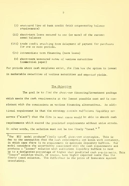
(i) unsecured line of bank credit (with compensating balancerequirements)

(ii) short-term loans secured to one (or more) of the currentasset balances

(iii) trade credit resulting from delayment of payment for purchasesfor one or more periods.

(iv) intermediate term financing (term loans)

(v) short-term unsecured notes of various maturities(commercial paper)

For periods where cash surpluses exist, the firm has the option to invest

in marketable securities of various maturities and expected yields.

The Objective

The goal is to find the short-run financing/investment package

which meets the cash requirements at the lowest possible cost and is con-

sistent with the constraints on various financing alternatives. An addi-

tional requirement is that the strategy contain sufficient liquidity re-

serves ("slack") that the firm in most cases would be able to absorb cash

requirements which exceed the predicted requirements without undue strain.

gIn other words, the solution must not be too finely "tuned."

The RTJ model produces" finely tuned" short-run strategies. This isdue to the assumption that the cash requirements are known with certainty,in which case there is no requirement to maintain liquidity buffers. Ourmodel considers the uncertainty associated with the cash requirements andproduces a "looser" solution with sufficient liquidity buffers to meetup to a designatea percentage of higher than predicted cash requirements. This"looser" solution would, of course, have higher expected costs than thefinely tuned solution. The difference is the price of insurance againstuncertainty.

10

III. A SAMPLE PROBLEM''"^

A sample problem is included at this point for several reasons-

to give the reader a better grasp of the type of problems being considered,

to make explicit the types of data required by the model and to serve as

the basis for examples of model equations in section IV.

The sample problem is to develop the optimal short term financial

plan, month-by-month, for a twelve-month planning horizon. The data for

the example is based partly on table 1 and partly on the description of

the financing options given below.

A. The Cash Budget

The month-by-month expected cash requirements are given in line

15 of the Cash Budget (table 1). These are the amounts which are projected

to be required in each sub-period of the planning horizon.

The realized values however will typically differ from the fore-

casted values. The uncertainty associated with the predicted requirements

results from the uncertainty associated with factors affecting the component

cash flows. For example, if sales were 10 percent higher than expected,

the pattern of net cash requirements could differ substantially from the

predicted values.

Given subjective estimates of the uncertainties associated with

the cash flow components, measures of uncertainty associated with the net

cash requirements can be obtained either analytically or through the use

The sample problem is an extended version of the RTJ case study in [1].

11

of simulation techniques. For most practical cases, measures of the un-

certainty of future cash requirements would be obtained by simulating the

cash budget and observing the distribution of possible values of the re-

quirements (lines 15 or 16).

We assume that the necessary simulations have been carried out

and the estimated standard deviations for the cumulative cash requirements

are given in line 17 of table 1.

B, Financing Alternatives

It is assumed that there are five financing alternatives open to

the financial officer. The amounts of financing available and the costs

of each source are described below. In the description of the alternatives,

it is assumed that all cash transactions take place at the beginning of

the decision periods.

1. Pledging of accounts receivable

The firm can pledge its accounts receivable as security for a

bank loan. The amount outstanding under this alternative is limited to a

maximum of $3,750,000. The bank will lend up to 80% of the face value of

the average amount of pledged receivables during any month. The cost of

borrowing under this alternative is 9.0% per year (0.75% per month) on

the amount of the loan outstanding during the month.

The liquidity buffer constraints are formulated on a cumulative basis.Thus, the standard deviations of the cumulative as opposed to non-cumulativerequirements are needed. The reasoning for this will be discussed inSection IV.

12

2. Unsecured Line of Credit

The company has available an unsecured line of credit from a com-

mercial bank which permits it to borrow up to $1,500,000 at an interest rate

of 8.5% per year (0.71% per month). The bank requires the company to main-

tain a compensating balance of not less than 20% of the amount actually bor-

rowed. However, 100% of the firms operating cash balance (line' 18, table l)

may be used to meet this requirement.

3. Stretching of Payables

The financial officer has the option to delay payment for purchases.

This will result in additional financing being supplied to the firm from

its vendors. If payments for purchases are delayed, the trade discouiits

allowed by the vendors will be lost. The discounts on the average amount

,to 3 1/2 percent of the face value of the bills. The firm can delay up

to 80 percent of the payables first due in any month for one month, and

60 percent for two months. Stretching for the second month involves no

further loss of discounts.

To the extent that stretching of payables generates vendor ill -

will, the cost of this option must be adjusted upward to allow for this

factor. Thus, the explicit cost (discounts lost) must be increased to meas-

ure the harm of possibly less favorable future service or credit

terms from the firm's vendors.

In the sample problem the implicit cost of vendor ill -will is

assumed to be 1 percent per year (0.08 percent per month) for payables

stretched one month and 10 percent per year (0.83 percent per month) for

12payables stretched an additional month.

12The implicit cost factors do not result in cash requirements during theplanning horizon, (i.e. they do not appear in the sources and used con-straints) but are included in the objective function to bias the selectionof financing sources away from this option.

13

Thus, if a bill for $1,000 (discounted value $965) is delayed

two months, the explicit financing costs would be 3.6 percent (based on the

discounted value) in the first month and percent in the second month.

The implicit costs would be o.083percent for the first month ($0.8) and

0.83 percent for the second month ($8.3). Thus, to obtain $965 for two

months, the total cost would be $4^-, which is equivalent to an annualized

borrowing rate of approximately 27 percent.

4. Term Loan

The firm has an offer of a term loan from its bank. The loan is

available only at the beginning of the initial period, and is limited to

a maximum $2,500,000. The principal of the term loan must be repaid in 10

equal installments beginning the seventn month with subsequent installments

due at six month intervals. No speedup in repayment is permitted. The

interest rate on the term loan is 10 percent per year (0.83 percent per

month) .

In addition the bank requires certain restrictions on the company's

operations, such as limits on capital expenditures, financing actions, etc.

These restrictions tend to reduce the flexibility of management during

the period of the loan, and thus generate implicit costs in addition to the

interest payment, as in the case of the stretching of payables option. Thus,

it is again appropriate to assign an additional cost factor to this option

in recognition of these intangible costs.

In the sample problem the term loan is assumed to carry an implicit

interest cost of 2 percent per year (0.17 percent per month).

14

5. Commercial paper

The firm has the option to issue 30, 60 and 90 day commercial

paper. The maximum amount which can be outstanding in any month (including

accrued interest) in $1,000,000.

The cost schedule (including issue costs) is 9.2, 9.0 and 8.8

percent per year for 1, 2 and 3 month commercial paper respectively.

Joint Borrowing Constraint

Further constraints are placed upon the firm's ability to borrow

from several sources at the same time. Specifically, the total borrowing

from all sources (excluding stretching of payables) is not to exceed

$4,000,000 in months 1 through 8 and $4,500,000 thereafter.

C. Short Term Investment Alternatives

The firm has the option of investing excess cash in either 30,

60 or 90 day securities. However, to insure a high degree of liquidity,

at least 50 percent of the marketable securities portfolio must be invested

in 30 day securities.

The yield schedule (net of transactions costs) is 7.0, 7.4 and

7.8 percent per year for 1, 2 and 3 month securities respectively.

D. Initial Conditions

Table 2 shows the initial values for the various asset and lia-

bility accounts as of the beginning of the planning horizon (before the

13first month's decisions).

13Repayments of any initial loans from commercial paper and term loan optionsare assumed to be included as part of the input cash requirements (line15 of table 1).

15

The "other current asset" and "other current liability" balances

are assumed to remain at their initial values throughout the planning

horizon.

E. Liquidity Reserve Requirements

Management wishes to insure that a sufficiently large liquidity

buffer is built into the financial plan to provide a specific degree of

protection against the uncertainties associated with the cash requirement

projections. The liquidity reserve is to be composed of marketable securi-

ties and unused short term borrowing potential (line of credit, secured

loans, stretching of accounts payable and commercial paper). The purpose of

the reserve is to insure that funds will be potentially available to the firm

in excess of the expected cumulative redjuirements (line 16 of table 1) in

amounts related to the uncertainties of the projected figures.

The following requirements describe the liquidity reserve to be

held in each month of the planning horizon.

(i) The minimum value must net be less than $500,000.

(ii) At least 50% of the minimum liquidity reserve must be heldin marketable securities.

(iii) Management is willing to take no more than a 10% risk of notbeing able to meet the cash requirements in any period fromplanned sources (funds raised to meet expected requirementsplus funds available from liquidity reserves)

.

16

Table 2

Summary of Initial Conditions

BALANCE SHEET AT BEGINNING OF PLANNING HORIZON

(thousands of dollars)

Current Assets :

CashMin. Operating Balance 100Additional Compensating Balance

100

Marketable Securities1-period maturity 2502-period maturity3-period maturity 500Total 750

Notes & Accounts Receivable 3000

Other Current Assets 4000

Total Current Assets 7850

Current Liabilities ;

Accounts PayableNot due in periodPayables delayedTotal

Commercial Paper1-period maturity2-period maturity3-period maturityTotal

Lines of CreditLoans secured by Accounts ReceivableTerm Loan

CurrentNon-CurrentTotal

Other Current Liabilities

Total Current Liabilities

700

17

F. Current Ratio Constraints

To obtain the financing terms described above, management

had to agree to maintain a current ratio (current assets/current liabili-

ties) of at least 1.2 during each period of the planning horizon.

G. End Conditions

The short term planning model only looks ahead for a finite

number of periods (typically 12 months) whereas the firm will continue

well beyond this time. Thus, it is necessary to insure that the recom-

mended capital structure at the end of the planning horizon be consistent

with operations beyond that point.

A problem can arise if we make no attempt to interface

the planning horizon of the model with the periods beyond. The model's

recommendations might leave the firm in such an illiquid state that

it would be unable to cope with the requirements beyond the planning

horizon.

There are a number of competing ways of treating this problem.

One is to insure that substantial liquidity reserves exist in the tenriinal

period. Another would impose terminal period current ratio constraints.

14These considerations are also important even in the cases where only the

model's first period decisions are to be implemented since these decisionscan be adversely affected by a myopic view of the life of the firm.

18

thus insuring expected terminal assets will exceed liabilities by a speci-

fied margin.

A third method is to constrain the terminal financial stru'-.ture

to a set of "reasonable" values. These values then constitute a target

short term financial structure for the model. A set of "end cost" para-

meters are used to penalize deviations from these target values. By

increasing the size of the end cost penalties, the terminal financial

structure can be made to approach any designated (but feasible) values.

For the sample problem, we assume the f ir r. has specified the target

balances and deviation costs shown in table 3.

Table 3

TARGET BALANCES & DEVIATION COSTS

Item

Pledged Receivables Loan

Line of Credit

Stretched Payables

Commercial Paper

Term Loan

Marketable Securities

Credit

Target

19

For example, if the tenninal period line of credit exceeds the

$200,000 target by $1,000, the cost of the solution would be increased by

$5.0. Note that in the case of securities, a credit is obtained for

balances above the target value.

H. The Objective

The firm's objective is to minimize total relevant costs, that

is, the sum of explicit financing costs plus any implicit costs associated

with deviations from the target financial structure. The optimization is

to be carried out subject to the limitations on financing sources, liquidity

reserves and current ratios.

We now proceed to the formulation of the mathematical programming

model which will produce the optimal short-term financial plan.

IV. MODEL FORMULATION

Before proceeding to the description of the model, we first sum-

marize the major assumptions that have been used in the development.

(i) The only uncertain quantity is the future cash requirements.

That is all of the uncertainty in the problem is confined

to the forecasts of the period-by-period cash requirements.

All other data (such as interest rates, receivables, payables,

etc.) are assumed known at the beginning of the planning hori-

zon. •'^

(ii) The financial manager is willing to specify the probability (e.g. 98%)

with which future (actual) cash requirements are to be met fromPlanned sources (including

This assumption allows us to deal with the major source of uncertainty in

the short term planning problem within a computationally feasible frame-

work. The other sources of uncertainty are typically of secondary im-

portance and would substantially complicate the solution procedures.

20

liquidity reserves) . The magnitude of this probability

(combined with the measures of uncertainty associated with

the cash requirements) will determine the magnitude of the

liquidity buffers to be maintained.

(iii) The firm is able to identify the complete set of financing

contracts available during the planning horizon. This de-

scription includes explicit financing costs, as well as esti-

mates of any intangible costs. The cost factors are assumed

to be directly proportional to the amounts borrowed.

(iv) The appropriate objective is to minimize the undiscounted sum

of expected financing costs (explicit plus implicit)

.

(v) The model is terminated after some finite number of decision

periods, but can be properly interfaced with the periods be-

yond the horizon such that the finite nature will have no

impact on the model's decisions. All transactions are assumed

to take place at the beginning of the decision periods.

While the assumptions regarding current knowledge of data from

future time periods may seem restrictive, this should not be the case in

practice, since typically only the first period decisions would be imple-

mented. The model would be re-run at the end of the first decision period

to prepare an updated plan using revised estimates of future cash require-

ments and financing costs. Thus, to the extent that forecasts change

during the first period of the planning horizon, the firm has the opportunity

to revise the second period decisions before they are implemented. The

liquidity buffer maintained during the first period leaves the flexibility

required to allow meeting of higher than expected second period cash

requirements or to permit smooth modifications of the remainder of the

short run plan.

Even though only the first period decisions are implemented, it

is necessary, however, to prepare the plan for the full short term planning

21

horizon. This results from the dependence of the first period decisions

upon expectations about conditions and courses of action in later periods

of the planning horizon. The first period decisions represent the optimal

first step in a multiple period short run plan based on the firm's best

estimates of future events and the uncertainty associated with future cash

requirements.

Using the assumptions discussed above, the short term financial

planning problem can be formulated as a linear programming model. Be-

fore proceeding with a detailed presentation, it is appropriate to first

summarize the structure of the model. The reader who is not inclined to

follow the complete description of the model can skip from the summary to

section V without loss of continuity.

A. Summary of the Model

The objective of the model is to minimize the total financing cost,

Z, over the planning horizon, where

Sum of Sum of

Explicit Implicit „ ,

Z = costs (interest + Costs + ^ ^T 1 4. A Costs

plus lost OverDiscounts) Horizon

Subj.ect to the following types of constraints.

(i) Constraints on the amount of financing available from each option;joint borrowing constraints on financing from several sources.

The problem is actually a stochastic programming problem, which can be

transformed into an ordinary linear programming formulation in severalways. The reasons for our choice of methods are discussed in note 1 of

the appendix.

22

(ii) Mix constraints on the marketable securities portfolio

(iii) Sources and uses constraints; expected sources of funds mustequal expected uses in each period.

(iv) Liquidity reserve constraints; the liquidity buffer must exceedminimum levels based on the uncertainty associated with the

forecasted cash requirements.

(v) Financial Ratio Constraints; the financial plan must maintain a

minimum current ratio in each period.

We now proceed with the details of the model. The constraints

of the model will be described first, followed by development of the object-

ive function.

B. Constraints on the Financing Options

The basic decision variables have the form X^^ and L^^ ' X^^

is the financing decision variable, representing the dollar amount of

financing outstanding from source i in period t. L,^^ is the contribution

of financing option i to the liqidity reserve in period t.

1 8Where the notation for any option differs from this format, it will be

described in the text.

22a

1. Pledging of Accounts Receivable

The loan available is limited to the minimum of $3,750,000 and 80

percent of the average receivables outstanding during the decision period.

Thus,

ht^ht 1 '"^^1 ,. „..^t-^^t+l

$3,750,000AR H

(0.8) [—^^ ^^]

t = 1, . . ., 12

where AR is the expected receivables balance at the beginning of period t,

(See line 1 of table l.)"*"^

2. Unsecured Line of Credit

The $1,500,000 unsecured line of credit with the 20 percent com-

pensating balance requirement generates the following constraints.

(a) Upper bound constraints

X2^ + 1-25L2J. <_ 1,500,000

t = 1, 2, . . ., 12

where L„ is the contribution of the unused line of credit to the liquidity

20reserve net of the full 20 percent compensating balance requirement.

19Since the values AR^ are assumed known for each period of the planning hori-zon, the minimum value of $3,750 and the average receivables can be computed(prior to execution) and inserted as the right hand side of the constraint

„^for each month.This is the most conservative assumption, since it assumes that no cashbalances will be available to support an additional line of credit. Thus, ifthe line of credit is increased at some future date to meet an unanticipatedcash requirement, only 80 percent of the amount borrowed is assvimed to beavailable to the firm.

The assumption is made here to simplify the exposition, and later in

section V for computational efficiency. The exact formulation, which considers

the cash balances available when computing L2t is described in note 2 of the append

22b

(b) Compensating balance requirement

C^ + b^ > 0.20(X2^.) ,

t = 1, 2, . . ., 12.

where

C = the proportion of the minimum operating cash balances

available to meet the compensating balance requirement.

(See line 18 of table 1.)

b = the additional amount borrowed at the beginning of period

t to meet the compensating balance requirement.

3. Stretching of Accounts Payable

The firm can stretch up to 80% of the payables first due in

any period for one month, and 60% for two months.

The constraints which limit the amount of payables which can be

21stretched one and two months are

St2 "^^3t2 -. 0.6AP^

,

t = 1, .... 12.

where

X„^ = the amount of payables first due in month t which are stretchedone month before payment (i.e., paid in period t + 1)

'•Note that the first constraint is an equality, rather than an inequality as inthe case of the previous financing options. This results from the fact that thestretching option does not enter into the joint borrowing constraint and thusthe liquidity reserve is equal to the slack on this constraint. This point willbe discussed further in connection with the joint borrowing constraint.

23

X„ „ = the amount of payables first due in period t which are delayed2 periods before payment

AP = the amount of payables first due in period t (See line 10 of table 1)

L_ = the contribution to period t liquidity reserve of unused stretch-

ing potential

L_ „ = the contribution to period t + 1 liquidity reserve of payables

delayed one period (i.e. due in t + 1) which can be furtherstretched into period t + 2.

For Loj.o to be a contribution to the liquidity reserve in period

t + 1, it is necessary that some amount of payables be stretched in period

t for planned payment in period t + 1 (i.e., X ^ > 0). ^ ^ must be no

larger than the minimum of X . and the difference between X and 0.6AP

^hus, a further series of constraints limiting the size of Loj.^

are required.

St2 1 Stl >t = l. . . ., 12 .

The oontribution of the stretching option to the period t liquidity

22reserve, Lo^» is given by

St = Stl-^h,t-l,2' t = l, . . ., 12,

For computational efficiency, only the L component of the stretching

liquidity reserve is included in the solutions shown in section V.

23a

The amount of accounts payable outstanding during month t (i.e.

after period t decisions have been made) , X , is given by

St = ^\ -^ Stl ^ St2 -^ S.t-1,2 t = l. . . ., 1]

where

PN = the payable outstanding but not due in period t (includes purchasesmade but not paid for in period t) (See line 9 of table i) .

24

4. Term Loan

The firm has the option of a $2,500,000 term loan in period 1, with

a 10 percent capital repayment requirement each 6 months thereafter.

23The limit on the term loan is given by

X, < 2,500,0004 —

The term loan decision variable is not subscripted since it is

assumed to be available only in period 1 of the planning horizon.

The amount of the term loan outstanding in period t is given by

a, X,, where a, is the proportion of the term loan outstanding in that period,

In the example, a,^ through a,, are equal to 1.0, a,^ through a.

= 0.90, a, - through a, „ = 0.80, etc.

5. Commercial pajjer

The finn has the option of issuing 30, 60 and 90 day commercial

paper. The value of commercial paper outstanding in period t (including

accrued interest), X^ , is given by

^5t = Stl ^ ^5t2 -^ St3

^ [^ ^ ^2^ S,t-1,2 ^ tl ^ ^3] S,t-1,3 ^ [^ - ^3^'S,t-2,3

t = 1, 2, .... 12,

23Note that the unused portion of the term loan has not been included as partof the liquidity reserve. This results from the assumption that increasingthe term loan will involve renegotiation with the bank and can not be ac-complished as quickly as obtaining funds from the other financing sources.

25

where

X^j.. = the amount of j period paper issued in period t, (j=l, 2, 3).

6 = the monthly interest rate for j period commercial paper (including amortisissue costs)

The constraints on the total amount of paper which can be issued are

given by

St "* St - 1,000,000 , t = 1, . . ., 12.

6. Total Borrowing Constraint

The maximum borrowing from all sources (excluding stretching

of payables) is not to exceed $4,000,000 in months 1 through 7 and

$4,500,000 thereafter. These restrictions are given by

ht ^ ht "^ ^4tS "^ St ^ ht ^ <^l-25)L2t "^ St - ^.000,000,

t = 1, . . .,7..

St * St "^ ^4tS "^ St "^ St "^ (1-25)L2^ + L^^ < 4,500,000,

t =8 , . . ., 12.

Note that the sum of the liquidity reserve contributions of the

pledging, line of credit and commercial paper options is constrained to be

less than or equal to the unused total borrowing capacity. Thus, if the

sum of the borrowings from these options is equal to the limit, they r.iake

no joint or individual contribution to the liquidity reserve, i.e.

St = St = St =°''

It is for this reason that the upper bound constraints on the individual

financing options were stated as inequalities rather than equalities. The

limit on line of credit in a given period, for example, may not be reached,

yet the option will have a zero L if the joint upper bound constraint

is binding in that period.

26

C. Marketable Securities Constraints

The firm has the option of investing in 30, 60 and 90 day se-

curities

The value of the marketable securities portfolio held during month t

(including accrued interest, net of transactions costs), X, , is given by

^6t " ^6tl + \t2 + ^6t3

^ fl -^ ^2^ \.t-l,2 ^ [^ -^ ^3^ ^6.t-1.3 -. [1 + \]\ ^ , ,3 b,t-2,3

t = 1, ... 12 .

where

X, = the amount of j period securities purchased in period t,(j=l,2,3)

p. = the monthly interest rate for j period marketable securities (net^ of amortized transactions costs).

The amounts of 1, 2 and 3 month securities outstanding

(X^^, j =1, 2, 3) are given by

4 = ^6tl ^ (^ ^ ^^2)^.^1,2 ^ (^ ^ V\.t-2.3'

4 = ^6t2-^ (^ + P3>^6.t-1,3'

3

^6t " ^6t3'

t = 1, 2, . . ., 12.

27

To insure that the portfolio remained highly liquid, it was required that

at least 50 percent of the portfolio be invested in the shortest maturity

securities. These portfolio mix constraints are given by

x] > X, ,

6t - 6t '

t = 1, 2, . . ., 12.

D. Sources and Uses Constraints

In each period of the model, the expected sources of funds must

equal the expected uses.

The expected cash requirements for each period, before any adjust-

ment for the costs of additional financing, are given in line 15 of table 1,

These requirements must be adjusted for additional interest expense, lost

discounts, interest earned on the marketable securities portfolio plus any

additional cash required for compensating balances.

These adjusted financing requirements must then be met via net

new borrowing (new borrowing less repa^/ments) plus net security sales in

each period.

Increases in the amount of any short term liability outstanding

or decreases in the value of securities held represent sources of funds

Conversely, decreases in short term liabilities or increases in security

balances represent uses of funds. For the problem to have a feasible sol-

ution, the amounts of short term securities and liabilities outstanding

must change in each period so that the net change is identically equal to

the adjusted requirements. Therefore, for each period (t = 1, . . ., 12)

we require

28

Additional

Expected ^^ .Cash re- Net

/-. -u .Financing

, „„.^„j ^^^ Net New _ ,Cash +P ^ ^ + quired for = . + Sales of

Requirements Compensating o w g SecuritiesBalances

(a) The expected financing costs in period t are the (cash) payments made

for all financing obtained in previous periods which matures in period t.

(i) Interest on receivables loan paid in t = r X

where r^ = the monthly interest rate

(ii) Interest on line of credit loan paid in t = r„X„

where r„ = the monthly interest rate

(iii) Discounts lost on payables stretched one and two periods

ago which are paid in t = r-[Xi

"*"

^3 t-2 2"'

where r„ are the discounts lost on stretched payables , expressed as a

proportion of discounted values

(iv) Interest on term loan paid in pe -iod t = r.a, ..X,4 4,t-l 4

where r = the monthly interest rate4

(v) Interest paid on commiircial paper issued 1, 2 and 3 periods

9ago which matures in period t = 6 X _ + [(1 + 6 )"-i.o]X

+ [(1 + V'-l-0]S,t-3,3

(vi) Interest earned on securities purchases 1, 2, and 3 periods

2ago which matures in period t = p^X, ^ , ^ + [ (1 + p^) -1.0] X, _ ,1 D,t-i,i 2 6,t-2,i

+ [(1+P3)^-1.0] X^^^_3^3

29

The net financing charges in period t are the sum of (i) through (v) less

(vi).

(b) The change in compensating balance requirement, which can not be met

with existing cash balances, is given by

(c) Net new borrowing in period t is given by

(X ~ ^1 _i

)

increase in receivables loan

+ (X - X _ )• increase in line of credit

+ ^Stl"" St2 - S,t-l.l

-h,t-2,2^

increase in stretched payables

+ (a, - a, t)X, increase in term loan^t A,t-i 4

+ (X^^^ + X^^^ + St3 " S,t-l,l " S,t-2,2 " S,t-3,3^

increase in commercial paper

(d) Net security sales are given by

^^6,t-l,l"^

^6,t-2,2"^

^6,t-3,3 " ^6,t,l" ^6,t,2" ^6,t,3^

E. Liquidity Reserve Constraints

The firm's liquidity reseirve is composed of the firm's marketable

securities balances plus the unused short-term borrowing capacity. The

unused capacity is included only if it can be assumed to be immediately

available without further negotiations. In the sample problem, this is

assumed to include all of the options with the exception of the term loan.

The liquidity reserve in period t, L , is given by

30

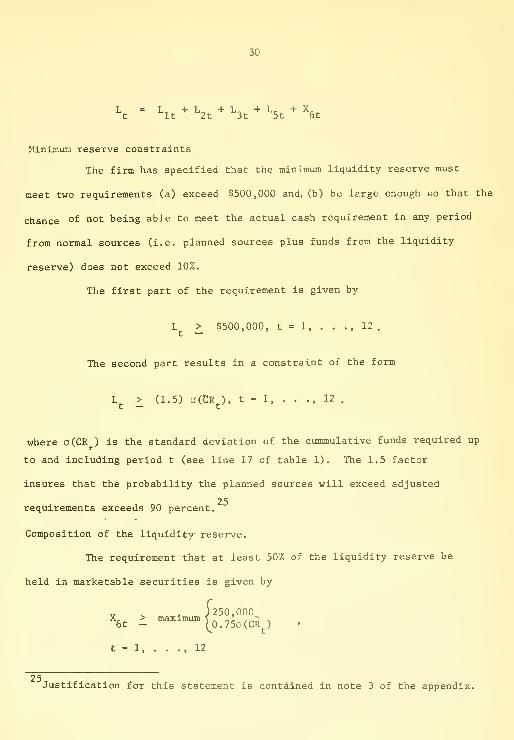
Minimum reserve constraints

The firm has specified that the minimum liquidity reserve must

meet two requirements (a) exceed $500,000 and, (b) be large enough eo that the

chance of not being able to meet the actual cash requirement in any period

from normal sources (i.e. planned sources plus funds from the liquidity

reserve) does not exceed 10%.

The first part of the requirement is given by

L _> $500,000, t = 1, . . ., 12 .

The second part results in a constraint of the form

L^ > (1.5) a(CRj.), t = 1, . . ., 12 .

where a(CR ) is the standard deviation of the cummulative funds required up

to and including period t (see line 17 of table 1). The 1.5 factor

insures that the probability the planned sources will exceed adjusted

25requirements exceeds 90 percent.

Composition of the liquidity reserve.

The requirement that at least 50% of the liquidity reserve be

held in marketable securities is given by

)250,000Xet i "'^^^'""^(o.75o(CR^) '

t = 1, . . ., 12

25Justification for this statement is contained in note 3 of the appendix.

31

F. Financial Ratio Constraints

It is required that the adopted financial plan maintain an expected

current ratio during the planning horizon of 1.2. This requirement is speci-

fied as follows

other current other[C + X.^ + AR^ + current] > 1.2[X. + X„^ + X.^ + term + X^ -r current

t ot t ^ — it It Jt -, 5t , . ^ .T . .assets loan liabilities

t = 1, . . ., 12 ,

where the current term loan is the sum of the installment payments due on

the term loan during the next 12 months (and thus by accounting conventions

a current liability)

.

G, The Objective Function

The objective function is made up of three cost components, the

explicit costs (interest and lost discounts) , the implicit costs assigned

to the intangible effects of the stretching and term loan options, and the

end costs associated with deviations of the ending working capital structure

from the designated target. The goal of the firm is to minimize the sum

of these costs during the planning horizon.

26As previously noted the liquidity reserve constraints, the current ratiorequirements and the end costs are all methods which can be employed toinduce a "reasonable" terminal financial mix. Since they tend to per-form overlapping functions, then obviously not all three are jointlyrequired in any problem. All have been included in the sample problemhowever simply to illustrate the most general formulation of the model.

32

The explicit costs in the objective function are computed on an

accrual basis (as opposed to the cash basis used in the sources and uses

constraints). For example, interest charges on loans outstanding are

charged to the periods for which the borrowing was in force and not to the

27periods in which the interest was actually paid.

The explicit costs associated with period t financing and In-

vestment decisions, E , are given by

^ = r^X^t + ^2^2t + ^3(^3tl"^ htl^ "^ ^^4t^4 "^ îStl

+ 6^X3^2 + ^3St3 - Plêtl - P2^6t3 - P3^6t3 '

t = 1 12 .

The implicit costs associated with period t financing decisions are

given by

^t = g3Atl -^ S32X3^,.i^2 -^ HÂth •

where g. = the intangible cost assigned to payables first due in

period t but stretched one period before payment.

= 0.083% per month

go^ = the intangible cost assigned to payables first due in

period t - 1 but stretched 2 periods before payment (and

thus providing additional financing in period t)

= 0.833% per month

g, = the intangible cost assigned to term loan borrowing

= 0.166% per month

The end cost associated with deviations from the target financial

structure, E, is given by

27Interest charges for financing options which exceed beyond the time horizonare truncated of the horizon (i.e., at the end of the twelfth period). Thus,

three period paper issued in period 12, would be charged only one period ofinterest in the objective function.

33

where X^ = the target balance for financing or investment option k

k = 1, . . ., 6.

h = the cost per dollar of deviation from the target balance

(see table 4 for the sample problem numerical values).

The objective function is thus to minimize, Z, where

12

Z =I (D^ + Dj.) + E

t=l

V. SOLUTION TO THE SAMPLE PROBLEM

The solution to the sample problem is presented in Figure 2 and

tables 4 through 7. After obtaining this solution, the sample problem

was modified by deleting the current ratio requirements and re-run. A

summary of this solution is shown in figure 3 and table 8. The reports

were produced by an interactive time-shared computer program called

SHORTER.^^

A. Description of Reports

Report #1: Borrowing Summary (See Figure 2)

27-,The SHORTER program is written in Fortran IV for use on the PDP-10 andIBM 360/67 time-shared computers. It is a self-contained package withinteractive input routines, a matrix generator, a linear programming sub-routine and a report generator. The report generator also produces sen-sitivity analyses for the objective function costs and the right handsides of the model constraints which have not been reproduced here forreasons of brevity.

3''

This report provides a period-by-per;-od summary of the amounts and

sources of the short term financing used in 'lach Jecision period. The

"period 0" figures shown relate to the amounts initially outstanding.

For example, in the second month of the planning horizon, the op-

timal plan contains $2,786,000 of short term financing, of which approximately

$2,000,000 comes from the term loan, $400,000 from stretching of payables

and $400,000 from the line of credit (precise figures for the amounts of

financing used are shown in tables 5 and 6).

The column labelled "ratio" gives the expected current ratio in

each month of the planning horizon. Note that the ratios in months 3 and

9 are as the minimum allowable values of 120.

Report #2: Cost Summary (See table 4)

This report summarizes the period-by-period accrued financ-

ing charges associate with the optimal financing decisions. The total

cost for the recommended financing and investment plan is $316,232,

which is made up of $267,278 of direct financing costs (interest expense

plus lost discounts) plus $48,954 of implicit costs associated with

stretching of payables, the term loan and deviations from the target fi-

nancial structure.

Report // 3: Sources and Uses of Funds (See table 5)^^

This report describes the optimal short-term financial plan. It

shows month-by-month how cash deficit s were financed and how cash surplus

were disposed of.

^ The reader should carefully distinguish between the accrued costs shown in

table 4 and the interest payments shown in table 5.

The cost summary corresponds to the terms in the objective function, i.e.

costs are assigned to periods in which the financing is outstanding

(i.e. accrued costs). For example, payables stretched for two periods in

month 6 would result in lost discounts charged to month 6 (accrued inter-

est column) plus implicit costs assigned to months 6 and 7.

The sources and uses statement is prepared on a cash flow basis. (It

corresponds to the expected sources and uses constraints in the

model). Thus, for example, in the above stretching example, the lost discounts

associated with the period 6 stretching would not show up on the sources and

35

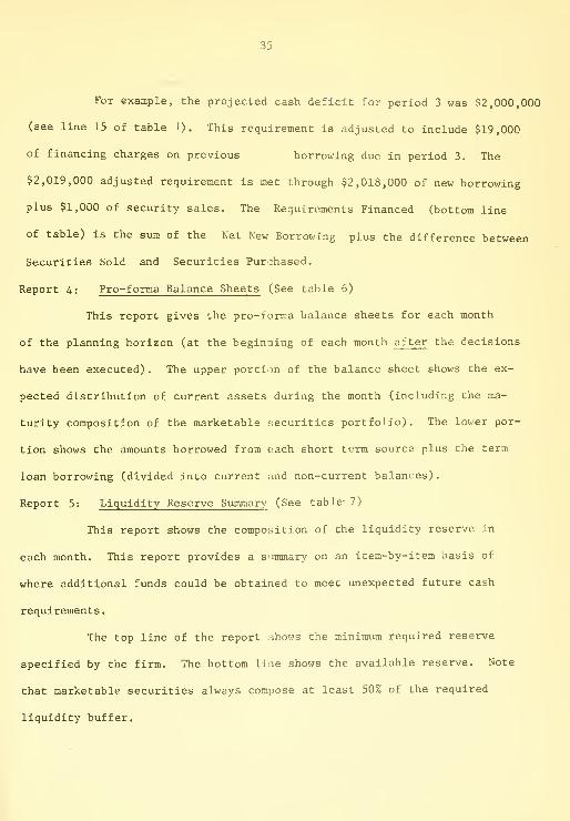
For example, the projected cash deficit for period 3 was $2,000,000

(see line 15 of table 1). This requirement is adjusted to include $19,000

of financing charges on previous borrowing due in period 3. The

$2,019,000 adjusted requirement is met through $2,018,000 of new borrowing

plus $1,000 of security sales. The Requirements Financed (bottom line

of table) is the sum of the Net New Borrowing plus the difference between

Securities Sold and Securities Purchased.

Report A: Pro-forma Balance Sheets (See table 6)

This report gives the pro-forma balance sheets for each month

of the planning horizon (at the beginning of each month after the decisions

have been executed) . The upper portion of the balance sheet shows the ex-

pected distribution of current assets during the month (including the ma-

turity composition of the marketable securities portfolio). The lover por-

tion shows the amounts borrowed from each short term source plus the term

loan borrowing (divided into current and non-current balances).

Report 5: Liquidity Reserve Summary (See table 7)

This report shows the composition of the liquidity reserve in

each month. This report provides a summary on an item-by-item basis of

where additional funds could be obtained to meet unexpected future cash

requirements.

The top line of the report shows the minimum required reserve

specified by the firm. The bottom line shows the available reserve. Note

that marketable securities always compose at least 50% of the required

liquidity buffer.

36

In period 1, for example, the required reserve is $500,000,

which is substantially surpassed by the actual reserve of $4,573,000. The

actual reserve is composed of $2,006,000 of unused pledging capacity, plus

$1,6CK>,000 of potential for delaying pa3rments for purchases (stretching) plus

$967,000 of marketable securities balances.

B. Analysis of the Solution

The major portion of the required financing is provided by the

term loan option, which at first consideration is surprising since this

option is the second most expensive (after one month stretching of payables).

The model recommends a $1,994,000 term loan in month 1, which is reduced

to $1,795,000 in period 7.

For the remaining requirements, the model makes use of all of

the sources at one time or other. The amount of the line of credit used

never exceeds 1,000,000 in periods where operating cash balances are $200,000

and $500,000 in periods where operating cash is $100,000. Thus, the model

only uses the line of credit where the compensating balance requirements

are covered by operating cash resulting in an effective interest cost of ortly

8.5 percent per annum.

The stretching option is only used in periods where the joint bor-

rowing constraint is binding (the reader will recall that stretching was not

included in this constraint). Thus, in period 3 for example, the total fi-

nancing used is 4,804,000 of whl<ch 804,000 comes from stretching of payables.

A similar situation exists in periods 4 and 9 where the joint borrowing con-

29straint is also binding.

29An exception is period 2, where stretching accounts for $400,000

of total financing. Total borrowing from sources other than stretchinghowever amounts to only $2,386,000 well below the $4,000,000 limit. Theresolution of this interesting paradox is left to the interested reader(However, see note ( 4) of the Appendix for a hint).

37

71gua:e 2 ~ BORROWING S^iT^AP.Y

PER RATIO TOTAL AMOUNT OUTSTANDING

0,001

2

3

4

5

6

7

8

9

101112

9435202474

712575

1,201,462,191.46

1250199427864804439039021994179527224849432323924500

SSSSSSSLLPPPTTTTTTTTTTTTTTTTTTTTTTTTTTTTTTTTTTTTTTTTS3SSLLLLTTTTTTTTTTTTTTTTTTTTCCCCCCCCCCSSSSSSSSLLLLLLLLLLTTTTTTTTTTTTTTTTTTTTCCCCCCCCCCSSSSLLLLLLLLLLTTTTTTTTTTTTTTTTTTTTCCCCCCCCCCLLLLLLLLLTTTTTTTTTTTTTTTTTTTTTTTTTTTTTTTTTTTTTTTTTTTTTTTTTTTTTTTTCCCCLLLLLTTTTTTTTTTTTTTTTTTCCCCCCCCCCSSSLLLLLLLLLLPPPPPPPTTTTTTTTTTTTTTTTTTCCCCCCCCCCLLLLLLLLLLPPPPPTTTTTTTTTTTTTTTTTTCCCCCCTTTTTTTTTTTTTTTTTTLLLLLPPPPPPPPPPPPPPPPPPPPPP

LEGEND:T =

C =

S =

L =

P =

TERM LOANCOMMERCIAL PAPERSTRETCHED ACCOUNTS PAYABLELINES OF CREDITPLEDGED ACCOUNTS RECEIVABLE

Table 4 — COST SUMMARY

PERIOD

37a

ta r^ s oj r<- to CM

s r- if> s h«- w r^

s r>. in ea r^ t\i <oT^ »-» to

IS to <a s r^ T-i t^

s s <s s t^ r^ o

to •r^ irv (s> s CM 1^

o< cr

CC — li. t I

o o a. uju. Lj z: Io q: <j) _i o I

CJ 2 < 2- O I

(_ o — — < zt/5 Z U X U O —

•

UJ — O O CK _JCC O I— UJ —UI Q UJ UJ 3: X CO>- UJ z cr s: or (/5

^ _J •-• t— O UJ UJ— Q. _J CO O »- _l

S I CO

t »ot I

t >©I in

Qo<

r th

37b

ea ta s CM if\ (M vo lA •* !S s s> s s IS la CM (a CM

ir IN. s o» tn ^o s (S> t (S I S G> S IS s s o 'S- ea 1^ s thO K)CVJ t^

in r^ ro IS in CM t> IS I ^ I

I >a I

I in I

IS CSk IS IS S (S ^ IS CM IS S >0

s '4^ s s cnr^ CM t CM I

t IS I

to S CM CM S f-^

•^^ la in >o cmr^ in ro in tH

(SI S O IS (9 sin 0003 CM

IS s C2 la in 03 r^ la I r~v I

I IS I

I in i

s la Q 1^ s r^ IS IS ta s (a ts

s s s IS ^^ o> o IS I o I

t la I

t in I

«a ta s> s s K' s Si ta la o o

O I O I

Z I O I

<t I — I

_J

37c

Table 6 — PRO FORMA BALajMCE SHEET

iT ASSETS:

J OPERATING BALANCE•L COMP BALANCEAL

37d

Table 6 (cont.) — PRO FORMA BALANCE SHEET

11

n assets:

J OPERATING BALANCE)'L COMP BALANCEFAL

37e

» -

38

The major question, however, relates to the use of the expensive

term loan option. Term loans carry a 10% per annum interest charge plus a

2% implicit cost. This results in a total cost per dollar borrowed

which exceeds all of the other options (except one-period stretching).

The clue to this puzzle comes from observing the current ratios

during the planning horizon. The solution is "binding" on the 1.20 minimum

during periods 3 and 9. The term loan is the only option that would allow

these constraints to be met. This results from the includion of only the

current portion of the term loan in the denominator of the current ratio.

Thus the term loan, in contrast to the other financing options, can be

used to sufficiently increase net working capital to meet the minimum current

ratio requirements.

The next question is how much does it cost the firm to meet the

minimum current ratio constraints. The answer is provided in figure 3 and

table 8, which show a summary of the same problem except for the deletion

of the minimum current ratio requirements.

The borrowing summary (figure 3) shows a radical shift in the fi-

nancing used. The term loan is no longer used, being replaced by primarily

a combination of commercial paper and pledging of receivables. The average

current ratio has declined. The former 1.2 minimum is now violated in four

months (2, 3, 4 and 9) reaching a minimum in month 3 of 0.99.

The cost summary (table 8) shows a $30,000 reduction in direct

financing costs, and an overall reduction of approximately $60,000 in the

total solution costs. The $60,000 figure provides management with a basis

for negotiation, if these constraints are externally imposed (i.e. try pay-

ment of higher interest rates to creditors to accept lower working capital

requirements) or a basis for deciding whether this "risk-avoidance" cost

38a

PER RATIO

Figure 3 — BORROWING SUMM-^sRY

TOTAL AMOUNT OUTSTANDING

0,00 i2!i0 :SSSSSSSLLPPP1 1.47 1265 SCCCCCSSSLLLLL2 1.05 2777 :CCCCCCSSSSLLLLLPPPPPPPPPPPPP3 0,99 4769 J CCCCCCCCCCSSSSSSSSLLLLLLLLLLPPPPPPPPPPPPPPPPPPPP4 1,01 4384 5CCCCCSSSSLLLLLLLLLLPPPPPPPPPPPPPPPPPPPPPPPPP5 1,33 3900 JCCCCLLLLLLLLLLPPPPPPPPPPPPPPPPPPPPPPPPP6 2.38 7 :

7 1,88 542 SCCCCC8 1,44 2076 5CCCCCCLLLLLPPPPPPPPPP9 1,02 4822 :CCCCCCSSSLLLLLLLLLLPPPPPPPPPPPPPPPPPPPPPPPPPPPPP

10 1,20 4309 '.CCCCCCCCCCLLLLLLLULLPPPPPPPPPPPPPPPPPPPPPPP11 1,61 2367 :CCCCCCCCCCLLLLLPPPPPPPPP12 1,22 4486 S CCCCCCCCCCLLLLLLLLLLLPPPPPPPPPPPPPPPPPPPPPPPP

LEGEND}T 8

C 3

S a

L s

P s

TERM LOANCOMMERCIAL PAPERSTRETCHED ACCOUNTS PAYABLELINES OF CREDITPLEDGED ACCOUNTS RECEIVABLE

Table 8 ~ COST SUMMARY

PERIOD

39

is justified if the constraints are internally imposed.

In this latter case, the additional protection provided by the

current ratio constraints over the liquidity reserve requirements might well

be questioned. The liquidity reserves were established to insure a minimum

probability that future cash requirements could be met from existing

sources of funds. The current ratio constraints attempt to duplicate this

function in a less direct manner and thus are probably not worth the sub-

stantial additional cost.

VI . SUMMARY

The model presented in this paper permits the financial manager

to incorporate his subjective estimates regarding the uncertainty of future

cash requirements into the development of the optimal short-run financial

plan. The liquidity reserve features of the model permit the maintenance

of any desired degree of protection against the possibility of not being

able to meet future cash requirements from planned sources of funds. The

liquidity reserve contains the firm's marketable securities balances plus

any unused borrowing potential on immediately available financing sources.

In most applications only the first period decisions would be

implemented. The model would be re-run at the end of each month using re-

vised estimates of future cash requirements and financing costs. It is

necessary, however, to prepare the complete short term plan since the first

period decisions will depend upon expectations about conditions and courses

of action in later periods of the planning horizon.

40

We expect the model to be a useful aid to management in the

development of short term financing decisions for any firm with an interest-

ing short run planning problem. By interesting we mean alternating periods

of cash surpluses and deficits, a variety of financing alternatives and

constraints and explicit requirements for protection against the uncer-

tainties of future cash requirements.

APPENDIX

Note (1)

The short term planning problem has been formulated as a chance

constrained programming problem. This approach was used instead of the

more desirable multi-stage linear programming approach, since the determin-

istic equivalent linear programming problem has the same sire and structure

as a deterministic version of the short-term planning model. Consequently,

the computational burden of the stochastic version is no greater than for

the deterministic version of the model. Also, the amount of information

required about distribution of the cash requirements is less for a chance

constrained as opposed to a multi-stage linear programming approach.

The principal weakness of chance constrained model is that it only

indirectly evaluates the consequences of violating a constraint. The

chance-constrained approach indicates no differential panalty between a

small and a large violation of a constraint. In other words, specifying

the correct values of the probabilities with which constraints can be vi-

olated should be part of the optimization problem.

Therefore, being faced with the choice between two approaches for

modeling a multi-stage decision process, we have chosen the chance con-

strained approach (with its restricted meaning of optimality) as opposed

to the multi-stage model (with its severe limitation on problem size).

By making this decision we can solve interesting problems that would be

beyond the bounds of computation with the multi-stage linear programming.

For a further discussion of stochastic programming methods, see

[4] , chapter 16.

Appendix

Note (2)

The following formulation will reduce the contribution to

the liquidity reserve by unused lines of credit by only the amount of

any incremental borrowing required to meet the compensating balance

requirement and not the full 20 percent.

(a) Upper bound constraints

^2t ^^^2t

"^'^2t^

1,500,000, t = 1, . . ., 12

where Y^ = the incremental borrowing required to meet compensatingbalance requirements oa L„

(b) Compensating balance requirements

C^ + b^ - S^ = 0.2(X2^), t = 1, . . ., 12.

where S is the excess cash available from operating balances after

existing compensating balance requirements are met. Note that S will

equal zero whenever b is greater than zero.

(c) Incremental borrowing constraints

S^ + Y^ 1 0.2[L2^ + Y^], t = 1, . . ., 12.

Note that Y^ will equal zero whenever S is greater than 0.20 (L2t-^

With this new formulation, L_ is now the contribution to liquidity reserves

net of any additional borrowing required to meet compensating balance re-

quirements.

Appendix

Note (3)

The stochastic constraint which is implicit in the liquidity

reserve requirement is given by

Prob {CR < CS^ + L^} > 1 - et — t t —

where CR = the cumulative funds requirements to period t (a random variable)

CS = the cumulative funds raised via short term financing to

period t (a deterministic variable)

L = Liquidity reserve in t (a deterministic variable)

£ = the maximum acceptable probability of default.

The constraint is formulated on a cu^nulative rather than a non-cummulativc

basis so that the statistical relationship among the period by period cash

requirements, R , can be explicitly considered. Also the cummulative formu-

lation avoids the problem of double counting the same liquidity reserve

against the liquidity requirements in several periods.

This constraint can be restated in terms of the normalized cumulative

probability function for CR

CS^ + L^ - e(Cr^)

a(CR^)

> 1 - e

CS^ + L^ - E(Cr^) >_ k(a(CR^))

where k = F (1 - e) is determined from the distribution form for CR or

from a non-parametric relationship, such as Tchebyschef f's inequality. In

the example it is assumed that CR is normally distributed, thus k «* 1.5.

Appendix

Note (4 )

To see why the model stretched in period 2, rather than 3, it

is necessary to consider the incremental borrowing costs of the various

options as well as the marginal costs associated with an additional dollar

of cash requirements in month 3. The following are the shadow prices

(marginal costs) for the sources and uses constraints for each period in

the planning horizon.

Marginal Costs(Dollars per Additional Dollar)

Mo. 1 Mo. 2 Mo. 3 Mo. 4 Mo. 5 Mo. 6 Mo. 7 Mo. 8 Mo. 9 Mo. 10 Mo. 11 Mo. 12

0.206 0.198 0.190 0.106 0.098 0.090 0.084 0.077 0.069 0.031 0.023 0.016

REFERENCES

1. Robichek, Teichroew and Jones, "Optimal Short Term Financing Decision,"Management Science , Vol. 12, No. 1, September 1965, pp. 1-36.

2. James C. T. Mao, "Application of Linear Programming to Short TermFinancing Decision," The Engineering Economist , Vol. 13, No. 4,

pp. 221-241.

3. A. A. Robichek and S. C. Myers, Optimal Financing Decision , PrenticeHall, Englewood Cliffs, New Jersey, 1965.

4. Harvey M. Wagner, Principles of Operations Research , Prentice Hall,Englewood Cliffs, New Jersey, 1969.

a linear programming model for short term financial

Documents