a learning-based model for imputing missing levels in...
TRANSCRIPT

A Learning-Based Model for Imputing Missing Levels
in Partial Conjoint Profiles
Eric T. Bradlow, Ye Hu, Teck-Hua Ho∗
January 26, 2004
∗Eric T. Bradlow (Email: [email protected]) is an Associate Professor of Marketing andStatistics and Academic Director of the Wharton Small Business Development Center and Ye Hu (Email:[email protected]) is a doctoral candidate of Marketing, The Wharton School of the University of Penn-sylvania. Teck-Hua Ho (Email: [email protected]) is William Halford Jr. Family Professor of Marketing,Haas School of Business, University of California, Berkeley. Professor Ho was partially supported by a grant fromthe Wharton-SMU Research Center, Singapore Management University. We thank David Robinson and YoungLee for their help in data collection and seminar participants at UC, Berkeley, Singapore Management University,University of Michigan at Ann Arbor, and the Marketing Science 2002 conference for their useful suggestions.

Abstract
A Learning-Based Model for Imputing Missing Levels
in Partial Conjoint Profiles
Respondents in a conjoint experiment are sometimes presented with successive partial
product profiles (i.e., profiles with missing attributes). The manner in which respondents
integrate available information from the current profile, information embedded in all previously
shown profiles (perhaps through memory recall), and their prior knowledge about the product
category, to impute values for missing attribute levels, is both theoretically interesting and
practically relevant. Theoretically, this investigation sheds light on how customers integrate
different sources of information in evaluating products with incomplete attribute information.
Practically, this study highlights the potential pitfalls of imputing missing attribute levels using
simple rules (e.g., an averaging model) and develops a better behavioral model for describing
and predicting customers’ ratings for partial conjoint profiles.
This research has two primary goals. First, we model how respondents infer missing levels
of product attributes in a partial conjoint profile by developing a learning-based imputation
model that nests several extant models. The advantage of our approach over previous research
is that our general class of imputation models infers missing levels of an attribute not only from
prior levels of the same attribute, but also from prior levels of other attributes (especially those
that match the attribute levels of the current product profile). To account for heterogeneity in
learning and conjoint part-worths across individuals, we estimate our model using a hierarchical
Bayesian approach.
A second goal is to provide an empirical demonstration of our approach, and to test whether
learning in conjoint studies occurs, to what extent, and in what manner it affects responses,
part-worths, and the relative importance of attributes. We show that the relative importance
of attribute part-worths can shift when subjects evaluate partial profiles. Such behavioral
distortion suggests that consumers may “construct” rather than “retrieve” part-worths and
hence consumers are sensitive to the order in which the profiles are presented (akin to context
effects in surveys). Finally, our results show that a consumers’ imputation process can also be
influenced by manipulating their “prior” information about a product category.
Keywords: Conjoint Analysis, Consumer Choice, Hierarchical Bayes Methods, Learning
Model.

1 Introduction
Conjoint analysis is perhaps the most celebrated research tool in marketing. It has been applied
to solve a wide variety of marketing problems ranging from understanding consumer preferences,
estimating new product demand, to designing a brand new product line. The method involves
presenting customers with a carefully chosen set of product profiles (called a test set) from the
universal set (as defined by the levels of the attributes) and collecting their preferences (ratings,
rankings, or choices) for product profiles in the test set. The power of the method lies in its ability
to extrapolate customers’ preferences from this test set to the universal set. Clearly, the conjoint
analysis method works better when the test set is small and the preference task difficulty is low.
Both factors can be significantly influenced by the number of product attributes.
If the number of attributes is large (as in many high-tech durable products), a full-factorial
experiment would require a respondent to assess their preferences for a large number of profiles,
each consisting of many attributes. The large test set problem can be solved by using a fractional
design (Plackett and Burman 1946; Green, Carroll, and Carmone 1978) that divides the test set
among several respondents within a common customer segment.
There are two ways to solve the task difficulty problem. The first way is to use a self-explicated
conjoint analysis (SECA) (Green 1984): consumers first rate the importance of the attributes, and
then evaluate the attractiveness of each attribute level. By multiplying the normalized importance
and attractiveness ratings, one can derive a consumer’s overall preference for any profile. This
approach typically requires the respondent to answer a smaller set of questions than a full profile
judgment task, and avoids the complexity of judging a profile with too many attributes. However,
the SECA method has its own problems, including the fact that attribute importance ratings by
respondents are not always consistent with their preference decisions; the experimental condition
of separating attribute and level ratings is artificial because real-life purchase decisions are made
on whole products.
The second solution is to use orthogonal subsets of all the attributes (Green 1974), the so-called
partial profile conjoint analysis (PPCA). Given that profiles with a smaller number of attributes
may be easier to rate (our experiment reveals that subjects took a significantly shorter time when
they were asked to rate partial profiles), the PPCA approach decreases the difficulty of the rating
task; however, at the same time, it may increase the number of profiles needed to determine
1

consumers’ utility functions. The PPCA approach typically assumes that the attributes that are
missing do not impact the product evaluation. Several studies cast doubt on this assumption (e.g.,
Feldman and Lynch 1987; Huber and McCann 1982; Broniarczyk and Alba 1994). Consequently,
standard rating conjoint analysis methods, applied to partial profiles, may not produce a highly
predictive utility function. This paper investigates how subjects impute missing attribute levels
when evaluating partial conjoint profiles. Our goals are to understand the dependency of ratings
of current profiles on all available attribute information (in both the current and previously shown
profiles), including a person’s prior knowledge, and to provide insights as to how consumers may
impute missing levels when evaluating partial conjoint profiles.
In this paper, we relax the “null effect for missing attribute” assumption and develop a prob-
abilistic model of how respondents impute values for missing attributes based on a person’s prior
over the set of attribute levels, a given attribute’s previously shown values, the previously shown
values of the other attributes, and the covariation between attributes (both a priori and learned
within the task itself). We conceptualize how consumers infer missing values via a pattern match-
ing and learning process. Our model assumes that consumers learn and update after each stimulus
(partial profile) about the pattern underlying the product attributes, their levels, and the cor-
relations between them. How are strengths of patterns formed and updated? We assume that
consumers have prior knowledge about the patterns and use knowledge about the product profiles
acquired through the conjoint task to update their strengths. It is this dynamic process (learning
about the attribute level occurrences and covariation between attributes) that we model and focus
on in this paper.
We call the fundamental kernel of this updating structure a “pattern matching” learning
model. That is, previously shown profiles that exhibit certain patterns among the attributes are
used by the respondent to infer the missing attribute levels in the current profile. In essence,
this approach can be viewed as a time-varying, multi-way contingency table of latent counts
for imputation. Consequently, the order in which profiles are presented matters in predicting
preference ratings.
We model how people rate partial conjoint profiles over time. While rating-based methods
may currently be less common than choice-based methods in practice (Wittink and Cattin 1989),
2

our study is relevant for common applications of conjoint analysis in at least three ways1:
1. Our research can influence the way that Adaptive Conjoint Analysis (ACA) is used in
practice. The ACA engine (for example, equation (2) in ACA 5.0 Technical Report) requires
continuous strength of preference data, treated as a rating score, obtained for pairwise partial
profiles. Although ACA can handle up to 30 attributes, it is suggested that each profile
should contain no more than five attributes, a practice which has been brought into question
by others (see for example, Green, Krieger, and Agarwal 1991; and subsequent response
Johnson 1991). Our work is directly applicable to the ACA engine, which selects profile
pairs based on utility balance, and, if those utilities are influenced by the missing attributes
that do not cancel across choice pairs due to covariation, learning, etc., the resulting part-
worths may be biased in some sense. Our model will help to quantify these biases or select
pairs that indeed have the highest likelihood of cancelling out on those missing attributes.
2. Our research has implications for the hybrid approach proposed by Srinivasan and Park
(1997) and subsequently extended by Ter Hofstede et al. (2002). That is, both share the
same data structure in which a subset of the most important attributes, based on self-
explicated data, is used in a subsequent “full profile” conjoint study. The phrase full profile
is in quotes because respondents are aware of all of the attributes before they rate the
profiles that contain only the subset of attributes. In this manner, one could consider the
profiles shown in their approaches “partial” and our model is able to shed light on the role
of those attributes that are excluded in the rating task.
3. Our study is also relevant for choice-based conjoint (CBC) methods despite the assumption
of ignorability across pairs of not shown attributes (Elrod, Louviere, and Davey 1992).
Conceptually, all profiles, even if stated as full profile, have missing attributes that could be
inferred. Therefore, despite the common practice of stating “respondents were instructed
that profiles were very similar in every respect except possibly for those attributes shown in
the profile description”, it is an open empirical question whether respondents do, or possibly
more importantly can follow this instruction. Hence our model can be used to check whether
indeed subjects are able to ignore levels of those attributes that are not included in the study.1We thank the editor and an anonymous reviewer for pointing out the link of our study to these approaches.
3

The rest of this paper is composed of four sections. In section 2, we develop our imputation
model. In section 3, the design of our experiment is explained. In section 4, we estimate our
model on two sets of experimental data and report the results. Section 5 contains conclusions,
caveats, and areas for future research.
2 The Imputation Model
2.1 Notation and Model Set-up
We investigate how I individuals (indexed by i = 1, · · · , I) rate a series of product profiles (partial
or full) in a conjoint experiment. Each product profile is characterized by J attributes (indexed
by j = 1, · · · , J) and each attribute j has two levels. Each individual i rates T profiles (denoted
by Mi(t), t = 1, · · · , T ) one-by-one. Individual i’s rating for product profile Mi(t) is given by
yi(t).
Profile Mi(t) takes a level of xij(t) = 1 or 0 for attribute j. We denote whether or not attribute
j is missing in the t-th shown profile to respondent i by rij(t). If attribute j is missing in profile
Mi(t), rij(t) is zero, otherwise rij(t) is 1. The basic premise of our model is that subject i does
not ignore a missing attribute level but instead constructs an imputed value for it. Let x′ij(t) be
that imputed value determined as follows:
x′ij(t) =
xij(t) if rij(t) = 1
Ixij(t) if rij(t) = 0
Note that Ixij(t) is a random variable, taking on the value of 1 or 0 (or in general the possible
values of xij(t)), and the imputation modeling effort is to determine its probability distribution
over the possible levels. If an attribute is non-missing (i.e., rij(t) = 1), it is assumed that the
shown attribute level, xij(t), occurs with probability 1.
To determine the part-worths of the attributes, we postulate a regression with heterogeneous
coefficients given by:
yi(t) = αi +J∑
j=1
βijx′ij(t) + εi(t) (1)
where βij is respondent i’s part-worth for attribute j.
4

Johnson, Levin, and their colleagues (Johnson and Levin 1985; Levin et al. 1986; Johnson
1987), however, suggest that subjects may have different part-worths for the same attribute when
it is missing compared to when it is not. To control for this, the above regression equation is
modified to yield:
yi(t) = αi +J∑
j=1
[βijx
′ij(t) + β′ijrij(t)
]+ εi(t) (2)
Table 1 shows the model’s part-worths under different conditions. If subjects indeed have different
part-worths when an attribute is missing, then β′ij will be significantly different from zero.
[Insert Table 1 Here.]
Thus, our model nests the work of Johnson, Levin, and others and generalizes theirs by including
imputed attribute levels x′ij(t) when rij(t) = 0.
2.2 Basic Ideas
Table 2 shows a hypothetical example that introduces the basic ideas of our imputation model,
as well as demonstrates current extant models. There are four attributes (i.e., J = 4) and three
profiles (i.e., Mi(1),Mi(2),Mi(3)). Each profile has one missing attribute (denoted as “MA”)
where subject i rates Mi(1), Mi(2), Mi(3) sequentially. At time t = 3, we have xi1(3) = 1,
xi3(3) = 1, xi4(3) = 0. Attribute 2 is missing at time t = 3 and we denote its imputed level, 1 or
0, by x′i2(3). In a real experiment, the respondent is shown a product profile at time 3 with only
attributes 1, 3, and 4, and does not see “MA” for attribute 2; we include it in Table 2 only to
describe the design.
[Insert Table 2 Here]
Assume that the subject has finished rating profiles Mi(1) and Mi(2), and profile Mi(3) is
the “current” product profile. To investigate how information from different attributes might
influence the imputed value for attribute 2 at time t = 3, we divide the attributes into three
types: 1) the omni-present (OM) set; 2) the presence-manipulated (PM) set that are present
(non-missing PM); and (3) the presence-manipulated set that are missing (missing PM). The OM
attributes are always presented while the PM attributes may or may not be. A PM attribute is
5

called a “non-missing PM attribute” if it is not missing in the current conjoint profile. A PM
attribute is called a “missing PM attribute” if it is missing in the current conjoint profile but
may not be missing in others. In profile Mi(3), attribute 1 is an OM attribute; attributes 3
and 4 are non-missing PM attributes; and attribute 2 is a missing PM attribute. Existing models
utilize only the past information (values) from the currently missing PM attribute (attribute 2) for
imputation of the missing level xi2(3). Our model uses all three sources, missing and non-missing
PM attributes and OM attributes.
There are several different existing ways to treat missing attribute levels. The first way is
to assume that respondents ignore them (Green 1974). Such an assumption implies that all the
“MA”s in Table 1 are filled in as 0 (the default level). Formally, this assumption leads to the
following prediction of the missing attribute level: Pr(x′i2(3) = 0) = 1 and Pr(x′i2(3) = 1) = 0.
Note that, in this case, the imputation process of the missing levels depends on which level is
coded as 0, a potential problem theoretically.
An alternative approach is to assume respondents impute values using all available information.
That is, we assume that people infer the levels of the missing attributes from previously shown
product profiles, and weight each profile “pattern” accordingly. This latter view is consistent with
Meyer (1981) where he shows that when a subject has no information about certain attributes,
that attribute is not ignored, but assigned a score equal to the individual’s adaptation level.
There are two common ways to model how consumers make inferences about missing attribute
levels. One way is based on the so-called “recency effect” (Lynch and Srull 1982): people assume
the missing attribute level to be the last level of the same attribute they saw. According to such
a model, in Table 2, attribute 2 in profile Mi(3) takes level 1 (following the level of attribute 2 in
profile Mi(2)). Formally, we have: Pr(x′i2(3) = 0) = 0 and Pr(x′i2(3) = 1) = 1.
A second commonly used imputation approach is the averaging model (Yamagishi and Hill
1981); people impute the missing attribute level by averaging all the previously shown levels of the
missing attribute. For example, in Table 2, this yields Pr(x′i2(3) = 0) = 12 and Pr(x′i2(3) = 1) = 1
2 .
In imputing the missing values, the recency and averaging models make strong assumptions
about the similarity between the current profile and the previous profiles. The recency-based
model assumes that the current profile is “similar” only to the most recently shown profile and
6
is dissimilar to the rest2. The averaging model assumes that the current profile is equally similar
to all the previously shown profiles. One would expect that some previously shown profiles are
more similar (“count more” in imputing) to the current profile while others are less so.
All the above models utilize only past data from attribute 2 to impute x′i2(3). By doing so,
they ignore two important pieces of information. First, there are the complete set of patterns
shown to the subjects (Mi(1), Mi(2)), not just the values for attribute 2 (xi2(1), xi2(2)). Some of
these patterns might occur more frequently, so their values for attribute 2 might be more salient
and memorable. Second, levels of other attributes from the current profile (i.e., Mi(3)) might
be diagnostic about the missing level. For example, if attribute 1 is negatively correlated with
attribute 2, as in Table 2, then one might infer from a 1 in attribute 1, a 0 for attribute 2. Such a
correlation structure could be based on people’s long-term memory or from the “learning” in the
conjoint task. Huber and McCann (1982) showed that people use their belief of the correlation
structure between price and quality to infer the missing price or quality when either one is missing.
Broniarczyk and Alba (1994) also show that consumers’ intuitions (priors) influence their inference
making. Our model captures these covariances as well as the priors they “arrive” at the experiment
with in a parsimonious way.
Like existing models, our imputation model derives probabilities that the missing PM attribute
2 in profile Mi(3) takes a value of 1 or 0. The parameterization of the probabilities is based upon
the work of Hoch, Bradlow, and Wansink (1999), which describes a similarity measure between a
pair of categorical objects (conjoint profiles in this research), and Camerer and Ho (1998, 1999)
and Ho and Chong (2003), which describe how learning and memory decay occur over time. The
two basic concepts we utilize here are what we call “Pattern Matching” and “Experience Counts”.
They are then combined to yield our imputation model which defines the probabilities over the
missing attribute levels.
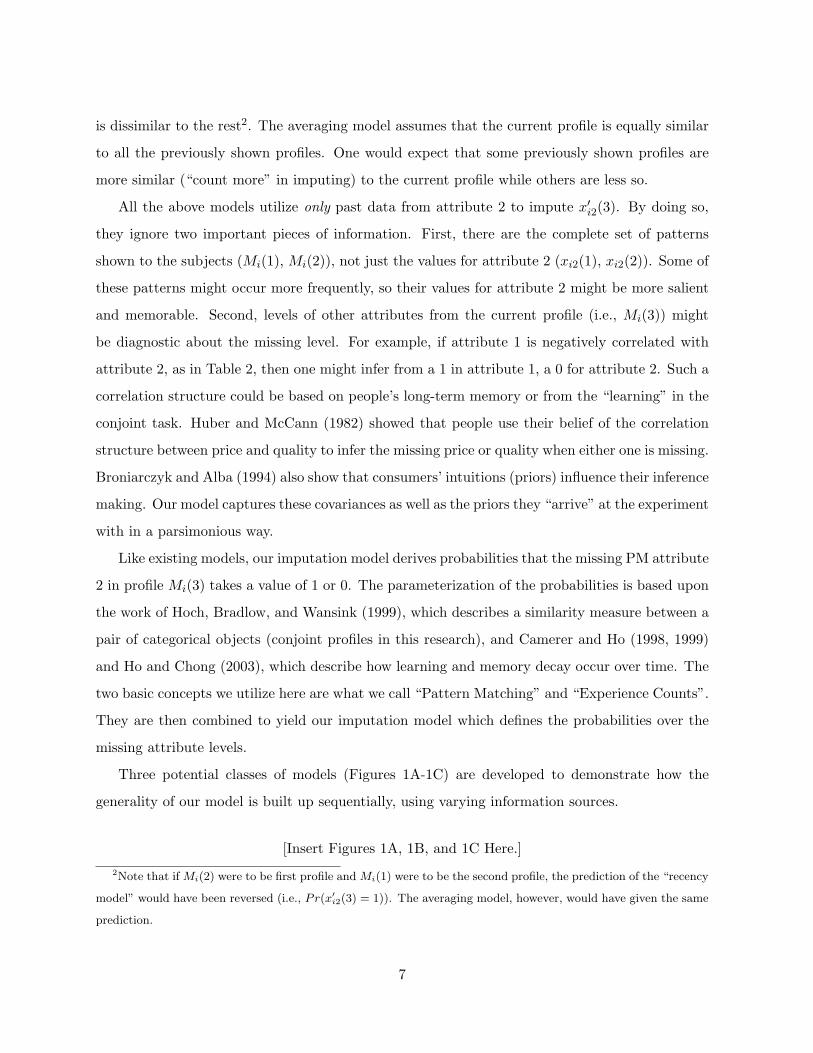
Three potential classes of models (Figures 1A-1C) are developed to demonstrate how the
generality of our model is built up sequentially, using varying information sources.
[Insert Figures 1A, 1B, and 1C Here.]2Note that if Mi(2) were to be first profile and Mi(1) were to be the second profile, the prediction of the “recency
model” would have been reversed (i.e., Pr(x′i2(3) = 1)). The averaging model, however, would have given the same
prediction.
7

The model in Figure 1A uses only previously shown information about the missing PM attribute
(i.e., j = 2) to impute missing levels. It is a natural extension of the recency and averaging model
that allows for decay. The imputation is based on historical levels of attribute 2 (0 in profile
Mi(1) and 1 in profile Mi(2)), but now with the more recent level (1 in profile Mi(2)) being
potentially more influential. To capture the “recency effect” in a “decay-weighed” averaging
model, we introduce a decay parameter, λ2 (0 < λ2 ≤ 1, the subscript denoting attribute 2). We
also introduce a new concept, “experience count (EC)” (Camerer and Ho 1999) such that Nij(t|l)denotes respondent i’s latent EC of attribute j at time t, taking level l.
As illustrated in Figure 1A, Ni2(3|0) = λ22 because Mi(1) has an observed level of 0 on attribute
2 at time 1 (i.e., xi2(1) = 0), and if x′i2(3) were to be imputed as a 0, λ2 gets a power of 2 because
there are two periods of time difference between profile Mi(1) and profile Mi(3) in which they
would then match on PM attribute 2. Similarly, Ni2(3|1) = λ2 because Mi(2) has xi2(2) = 1 and
would match with x′i2(3) if it were to be imputed as a 1. Therefore, the probability that x′i2(3)
takes level 1 or 0 is thus:
Pr(x′i2(3) = 1) =Ni2(3|1)
Ni2(3|1) + Ni2(3|0)=
λ2
λ2 + λ22
Pr(x′i2(3) = 0) = 1− Pr(x′i2(3) = 1)
The averaging model is a special case of this class of models in which λ2 = 1. The recency model
has λ2 → 0, with Pr(x′i2(3)) = 1) → 1 and Pr(x′i2(3)) = 0) → 0.
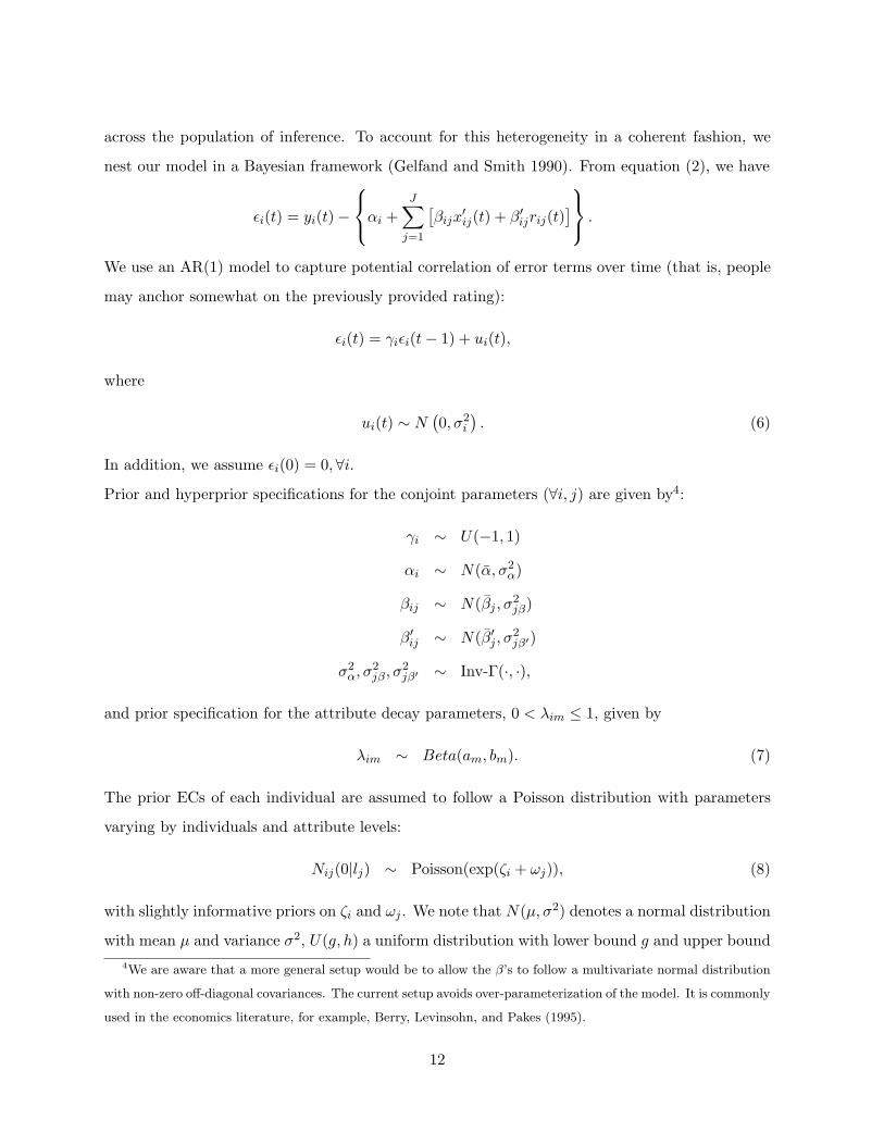
The more general model in Figure 1B uses information from both the missing and non-missing
PM attributes (attributes 3 and 4) for imputation. That is, in addition to using information
from attribute 2 itself, we utilize possible conditional match patterns between profiles on the
non-missing PM attributes. Since we assume that the missing attribute levels are not used for
imputation3, we only need to check whether there is a match between [xi3(3)] and [xi3(2)] and
between [xi4(3)] and [xi4(1)]. Since [xi3(3)] and [xi3(2)] match, we expect Mi(2) to influence
imputation more than Mi(1) on Mi(3). Another decay parameter, λ3 (0 < λ3 ≤ 1), is added to
capture this reinforcement. Consequently, Ni2(3|1) becomes λ2 + λ3, where Ni2(3|0) stays the3This is an assumption/limitation of our approach that is discussed later and is an area for future research.
8

same. The probabilities that x′i2(3) is imputed as 1 or 0 now becomes:
Pr(x′i2(3) = 1) =Ni2(3|1)
Ni2(3|1) + Ni2(3|0)=
λ2 + λ3
(λ2 + λ3) + λ22
Pr(x′i2(3) = 0) = 1− Pr(x′i2(3) = 1)
Notice that Pr(x′i2(3) = 1) becomes larger, when compared to Figure 1A, as Mi(2) (when com-
pared to Mi(1)) is more similar to Mi(3) than when we considered only the missing PM attribute.
The model in Figure 1C uses all of the available information from both the PM (missing as
well as non-missing) and OM attributes to impute the missing level. Following the procedure
above, the ECs are Ni2(3|0) = λ21 + λ2
2 and Ni2(3|1) = λ2 + λ3. The corresponding probabilities
now become:
Pr(x′i2(3) = 1) =Ni2(3|1)
Ni2(3|1) + Ni2(3|0)=
λ2 + λ3
(λ21 + λ2
2) + (λ2 + λ3)Pr(x′i2(3) = 0) = 1− Pr(x′i2(3) = 1)
The most general model, Figure 1C, has two desirable properties:
1. It uses all available information in the previously shown and current profiles in a sensible
way. Furthermore, the model highlights the potential pitfalls of the averaging and recency
models. For example, it implies that these previous simpler models will yield the same pre-
diction, given above, if Mi(3) were to take any of these patterns {[1,MA, 1, 1], [1,MA, 1, 0],
[1,MA, 0, 1], [1,MA, 0, 0], [0,MA, 1, 1], [0,MA, 1, 0], [0,MA, 0, 1], [0,MA, 0, 0]}, which seems
very unlikely.
2. It allows respondents to apply different weights to different attributes depending on their
preference.
2.3 General Formulation
In general, the pattern matching between two profiles can be formally defined as follows. Assume
rij(t) = 0 and the level of attribute j at time t for respondent i is to be imputed. For each
possible level of x′ij(t), we consider all previously shown profiles (t′ < t) that have attribute j
taking the same value (i.e., xij(t′) = x′ij(t)). That is, we find all t′ in which the indicator function
I(xij(t′), xij(t)) = 1. In addition, we set I(xij′(t), xij′(t′)) to 1 for those profiles Mi(t′) that have
9

a match along a different attribute j′ with the current profile Mi(t), but also on the missing PM
attribute j. We call this a conditional match-up model, as the pairs of profiles must match on
the missing PM attribute for it to add to the EC.
It is also important to note the following “properties” of our pattern matching approach. (1)
We do not match profiles based on imputed values of previous attributes, or in a more-than-one
missing attribute case, imputed values of missing PM attribute(s) j′ 6= j. (2) The way in which
we “match” a given pattern is binary (yes it matched, no it did not). One could imagine a
metric-based degree of matching model. We chose a binary Hamming metric approach as it is
parsimonious, easy to describe, and is cognitively simple.
Let Nij(t|lj) denote the latent EC of individual i for attribute j to take level lj at time t.
With attribute j as the missing PM attribute, our model for Nij(t|lj) in complete generality is
given by
Nij(t|lj) = Nij(0|lj) + (3)t−1∑
t′=1
λt−t′
i(j,j) · I(x′ij(t), xij(t′)) +J∑
j′=1,j′ 6=j
[λt−t′
i(j,j′) · I[xij′(t), xij′(t′)
] · I [x′ij(t), xij(t′)
]]
= “prior count” + {“missing PM count” + [“non-missing PM attribute + OM attribute count”]}where Nij(0|lj) denotes the “prior” count of person i on attribute j, level lj at “time 0” and
0 < λi(j,j′) ≤ 1 is the decay parameter for person i relating attribute j′ (j′ = 1, ..., J) to j.
Nij(0|lj) allows for the possibility of prior knowledge of the marginal frequency of attribute levels
and prior correlation between attribute levels.
In our experimental results, section 4, we fit a fairly general (reduced-form) version of the
model (Equation (3)) that has the following set of specifications for λij . This corresponds to
Table 3, an example with digital cameras in which j = {1, 2, 3, 4} are PM attributes (delay
between shots, storage media, maximum resolution, and camera size) and j = {5, 6} are OM
attributes (price and mini-movie).
λi(j,j′) = λij if j′ = j, j′ ∈ PM ; ∀j = 1, 2, 3, 4
λi(j,j′) = λi5 if j′ 6= j, j′ ∈ PM
λi(j,j′)) = λi6 if j = Maximum Resolution and j′ = Price
Note that λi6 is included in the model, as described in section 4, due to a prior manipulation of
10

the covariance between price and maximum resolution.
[Insert Table 3 Here]
The structure described above defines the entire imputation process for partial profile conjoint
designs as a time varying latent contingency table with counts, Nij(t|lj), given in Equation (3).
Hence, Pr(x′ij(t) = lj), lj = 1 or 0, is given by
Pr(x′ij(t) = lj
)=
1 if rij(t) = 1 and x′ij(t) = lj
0 if rij(t) = 1 and x′ij(t) 6= ljNij(t|lj)
Nij(t|0)+Nij(t|1) if rij(t) = 0
(4)
That is, the probability a given attribute level is imputed, when that attribute is missing, is
its “proportion” of the total EC for that attribute. As Nij(t|lj) incorporates information across
patterns to reinforce each pattern, and allows for differing importance across time, this model
satisfies our basic pattern matching and reinforcement requirements. When there are multiple
attributes missing, we assume independence of counts to derive the joint probability of the missing
pattern; however the counts are correlated as attribute levels that occur together have counts that
will be updated together, and prior counts that are related.
We denote the vector of imputed values at time t by a row vector x0i(t) = [x′i1(t), x′i2(t), ...,
x′iJ(t)]. For a conjoint design with J attributes, where each attribute has two levels, the imputed-
value vector x0i(t) may assume one of the K = 2J possible potential profiles. We denote these
potential profiles by Zk (k = 1, ..., K) and we determine the probability that x0i(t) equals potential
profile Zk as
Pr(x0i(t) = Zk
)=
J∏
j=1
Pr(x′ij(t) = lj
). (5)
2.4 Heterogeneity
We allow for the rate of information decay for a specific attribute pattern to be individual and
attribute specific, recognizing that considerable heterogeneity is likely to exist across persons in
their decay attribute imputation parameters, λim (m = 1, ...6). In addition, the basic parameters
of the conjoint model, the individual conjoint intercepts, αi, the attribute part-worths, βij and β′ij ,
and the residual variances, may also contain considerable heterogeneity, yet share commonalities
11
across the population of inference. To account for this heterogeneity in a coherent fashion, we
nest our model in a Bayesian framework (Gelfand and Smith 1990). From equation (2), we have
εi(t) = yi(t)−αi +
J∑
j=1
[βijx
′ij(t) + β′ijrij(t)
] .
We use an AR(1) model to capture potential correlation of error terms over time (that is, people
may anchor somewhat on the previously provided rating):
εi(t) = γiεi(t− 1) + ui(t),
where
ui(t) ∼ N(0, σ2
i
). (6)
In addition, we assume εi(0) = 0, ∀i.Prior and hyperprior specifications for the conjoint parameters (∀i, j) are given by4:
γi ∼ U(−1, 1)
αi ∼ N(α, σ2α)
βij ∼ N(βj , σ2jβ)
β′ij ∼ N(β′j , σ2jβ′)
σ2α, σ2
jβ , σ2jβ′ ∼ Inv-Γ(·, ·),
and prior specification for the attribute decay parameters, 0 < λim ≤ 1, given by
λim ∼ Beta(am, bm). (7)
The prior ECs of each individual are assumed to follow a Poisson distribution with parameters
varying by individuals and attribute levels:
Nij(0|lj) ∼ Poisson(exp(ζi + ωj)), (8)
with slightly informative priors on ζi and ωj . We note that N(µ, σ2) denotes a normal distribution
with mean µ and variance σ2, U(g, h) a uniform distribution with lower bound g and upper bound4We are aware that a more general setup would be to allow the β’s to follow a multivariate normal distribution
with non-zero off-diagonal covariances. The current setup avoids over-parameterization of the model. It is commonly
used in the economics literature, for example, Berry, Levinsohn, and Pakes (1995).
12

h, Inv-Γ(·, ·) an inverse gamma distribution with corresponding parameters and Beta(a, b) a beta
distribution with parameters a, b. To complete the model specification, slightly informative hyper-
priors were placed on σ2α, σ2
jβ , and σ2jβ′ , ∀j (inverse gamma distribution: Inv-Γ(0.001, 0.001)); βj
and β′j , ∀j (normal distribution: N(0, 0.001−1)); and (am, bm) (uniform distribution: U(0, 1000)).
Numerous sensitivity analysis indicated that the results were not affected by the exact choice of
uninformative hyperprior values.
To summarize, let the imputation model parameters be denoted by row vectors λi = [λi1, λi2, ..., λi6]
(the length of λi varies with different models as described in section 4), and conjoint parameters
by βi = [βi1, βi2, ..., βi6], and β0i = [β′i1, β′i2, ..., β
′i6]. Given Pr(x0i(t) = Zk) from equation (5), the
likelihood function is
L(αi, βi, β0i,λi, γi, σ
2i ; yi) = (9)
20∏
t=1
26∑
k=1
1√
2πσ2i
exp
(−([εi(t)|Zk]− γiεi(t− 1))2
2σ2i
)· Pr(x0i(t) = Zk)
.
That is, we integrate the conjoint regression model with respect to the imputation model, i.e.
stick in the considered value for attribute j to person i for all possible profiles, and weight them
by their probability of being the imputed corresponding level. We use the notation [εi(t)|Zk] to
emphasize that the value of εi(t) is conditional on profile Zk. Also note that, although there are
26 potential profiles in our study, at each time t, only two profiles have non-zero Pr(x0i(t) = Zk)
in the one-missing attribute case and only four in the two-missing attributes case.
Inferences from all models were derived by obtaining posterior samples using a Markov chain
Monte Carlo sampler. All computation was performed using the software package WinBUGS,
Bayesian Inference Using Gibbs Sampling (http://www.mrc-bsu.cam.ac.uk/bugs/)5. All of the
results reported in section 4 are the posterior means obtained from aggregating the draws of three
runs of the sampler from different starting points with a burn-in period of 6000 draws, and a total
run length of 10,000 draws. Convergence was assessed using the F-test approach of Gelman and
Rubin (1992).5To assess the ability of our most general model (Model 6) in recovering the true underlying model structure,
we ran a simulation study using synthetic data. The simulation results indicate that the model is able to recover
the underlying conjoint regression coefficients (αi, βij , β′ij , and γi) very accurately and the imputation parameters
(λ’s) with reasonable accuracy. Details are available from the authors upon request.
13

Due to the complexity of the model, the fact that many readers may lack familiarity with
the WinBUGS software program, and a desire for other researchers to easily apply our model,
we have included an annotated version of the WinBUGS code for our most general model in an
online appendix at http://mktgweb.wharton.upenn.edu/ebradlow/research files.htm.
3 Experiment
An experiment was designed to provide a basic demonstration of our model on rating conjoint
data with missing attributes. Our interest lies in providing a demonstration of our approach, as
well as to begin a preliminary understanding of:
1. Do people use missing attributes, and their levels, to evaluate products?
2. If yes, do they infer missing attribute levels from all of the information they learn about the
product profiles; do they reinforce patterns?
We assume that a consumer has minimal prior information about the product, although we
do estimate this as given in Equation (8). Therefore, we are able to impose a “prior” structure
that varied across respondents in a systematic way (described below). First, through a learning
process, we create a “prior” for each individual by controlling the products that she sees in a
“learning phase”. Second, we ask participants to rate products with (or without, in the control
group) missing attributes. A second control group worked on a self-explicated conjoint task to
act as a second baseline.
3.1 Stimulus
Digital cameras were selected for this experiment as we wanted a relatively new product category
where the frequency of attribute levels and the correlation structure of the attributes are mostly
unknown. This would allow us to manipulate the frequencies and impose a prior as desired. From
our demographic questions, less than 10% of our subjects owned digital cameras or claimed to
have extensive prior expertise. We chose digital cameras with 6 attributes (as the full profile
task) as research that we conducted indicated that digital cameras could be described well using
6 features. A summary of the digital camera attributes used are listed in Table 3. In our
14

experimental condition, all attributes are simplified to have two realistic levels (note SLR =
single-lens reflex camera, a size bigger than medium). This product set-up provides a stylized
empirical test of our model.
3.2 Experimental Groups
The experiment was designed to run on a university network. One hundred and thirty undergrad-
uate students from a large east-coast university participated in the experiment. Subjects were
obtained and assigned to treatments by taking six sections of a large class and randomly assigning
one section each to receive the self-explicated and full profile (0 missing) cases, and two sections
each to receive the one missing and two missing attribute cases. This resulted in four groups with
group sizes 17, 23, 47, and 43, respectively6. Group size differences were due to different section
sizes and the participation rate of students in those sections. Across the conditions, less than 10%
owned digital cameras; 40% are females and 60% are males.
The experiment was composed of two phases: the learning (prior) phase and the rating phase.
In the learning phase, the subjects were provided with text information about digital cameras
and their attributes. They were then shown 20 digital camera profiles listed in a single table.
We control the consumers’ priors by manipulating the digital camera profiles they see in the
learning phase. In the rating session, the subjects were asked to rate, on a 0− 9 Likert scale, the
attractiveness of different digital cameras (some with partial product profiles depending on the
treatment condition).
3.3 Learning Phase
In the learning phase, all subjects were shown 20 digital camera profiles. The priors of the sub-
jects before the rating phase were manipulated by the learning phase profiles. The purpose of this
learning phase manipulation is two-fold. First, if the relationship say between price and maximum
resolution, as described next, can be influenced by showing subjects profiles of a given structure,
then managerial practice would suggest prior manipulations of this type could be valuable. Sec-
ondly, we wanted to test out our model, for a given attribute correlation. As we manipulated6We note that a better design would have been to randomly assign people and not sections. Experiment 2
utilized random assignment.
15

the priors between digital camera price and maximum resolution, we wanted to test if λi6 (as in
Section 2.3) would impact the EC for resolution when it is missing (price is never missing as it is
an OM attribute).
Each subject was randomly assigned to one of eleven prior coincidence structures representing
a different level of coincidence between price and maximum resolution (while keeping the coin-
cidences between other attributes orthogonal.) Specifically, they were assigned to read a table
with a specific coincidence value (between 0 and 10) between price and maximum resolution. For
example, a coincidence value of 10 indicates that among the 10 profiles that have low price ($159),
all have low resolution (800× 600); a value of zero would indicate that among the 10 profiles that
have low price ($159), all of them have high resolution (1024× 768). Such coincidence structure
could potentially affect Pr(x′ij(t) = lj) if the learning phase carries over to the rating phase. That
is, we will test empirically the ability to manipulate the rating phase data by co-varying price
and maximum resolution at levels 0, 1, ..., 10 in the learning phase, and then estimating λi6 in our
model and seeing its correlation with the subject’s prior manipulation.
To ensure that subjects followed and attended to all information in the table of 20 learning
profiles provided, they were asked to count five of the pairwise coincidences after they had read
the tables. Among the five questions, one of them asked the subjects to count the coincidence
between price $159 and maximum resolution 800 × 600, the manipulated coincidence, while the
other four questions were randomly chosen to ask the subjects to count other coincidences. The
sequences of these questions were randomized so as not to bias the results. Their responses to
these questions suggested that they had paid attention to the coincidence counts.
3.4 Rating Phase
In the rating phase, the design is orthogonal. In the one or two missing attribute group, one or
two out of four PM attributes are removed from the designed conjoint cards, respectively. We
fixed two attributes to be OM as we wanted to see the impact of imputation of missing levels
on observed attribute part-worths. We utilized a Plackett-Burman Design (Plackett and Burman
1946; Green, Carroll, and Carmone 1978) to create the profile cards. The sequences in which the
profile cards were shown were generated randomly and varied across respondent. Each subject
saw 24 profiles in the rating phase. Debriefing questions after the experiments provided evidence
16

that the subjects do “notice” that attributes are missing and utilize this fact in their ratings.
Response time was recorded, which could be used as a proxy for the difficulty of the task. Each
response time was the time (in seconds) measured between successive rating score responses being
keyed in. An analysis of the response time data across missing attribute conditions (0, 1, and 2)
indicated that respondents in the two missing case, spent considerably less time than in either
of the other two cases (p < 0.01), corresponding to an average of 31 seconds less across the 24
profile rating tasks. No significant differences were found in response time between the zero and
one missing attribute conditions.
4 Results
We utilized the first 20 profiles for each subject to the calibrate model, and the last four as holdout
for validation.
We estimated a total of six models, with differing degrees of generality. These models are
grouped into four categories: (1) prior models, (2) imputation based on missing PM attributes
only, (3) imputation based on missing and non-missing PM attributes, and (4) imputation based
on the OM attribute (Price), missing and non-missing PM attributes. Table 4 shows these models
and their relationships for both the one and two missing attribute cases. The estimation was done
using the Bayesian hierarchical structure described in Section 2.4.
[Insert Table 4 Here]
Table 5 shows the relative performance for the six models. We show results for the three
extant models (ignore, recency, and averaging), as well as one model in each of the three classes
(Models 4, 5, and 6). For each model, we report (1) the log of the marginal likelihood as computed
by the log of the harmonic mean of the likelihood values (Congdon 2001, p475), and (2) mean
absolute errors (MAE), both in sample and out of sample. Using all three measures, our models
(Models 4-6) perform better than the prior models (Models 1-3). Specifically, Models 4 through
6 consistently perform better as more information is used for imputation.
[Insert Table 5 Here]
17

4.1 Imputation Based on Missing PM Attributes
As discussed above, the extant models assume that subjects either ignore the missing attribute, use
the most recent occurrence of a missing attribute, or compute the average of all past occurrences.
Out of models 1-3, the averaging model (Model 3) performs better in terms of log-marginal
likelihood and in- and out-of-sample mean absolute error (MAE). Model 4 relaxes the assumptions
of Model 3: it allows a separate λ for each missing PM attribute, which decays geometrically.
Compared to the averaging model, Model 4 performs better in terms of log-marginal likeli-
hood, in sample and out of sample MAE. Such results suggest that the relaxation of allowing
for heterogeneous geometric decay helps in terms of model performance and better captures the
actual rating process when missing attributes exist.
4.2 Imputation Based on Missing and Non-missing PM Attributes
The above class of model assumes that subjects impute a missing level of an attribute using only
information within that PM attribute. A natural extension is to account for covariation from the
non-missing PM attributes. In Model 5, we assume each attribute to take a different λ when it is
present and when it is missing; however, the value of λ is assumed to be common across all PM
attributes when they are non-missing. As indicated in Table 5, Model 5 fits better than Models
1-4 in terms of log-marginal likelihoods, in-sample MAE, and out-of-sample MAE.
4.3 Imputation Based on OM Attribute, Missing, and Non-Missing PM At-
tributes
To fully test the information used by the subjects when inferring missing attribute levels, in
addition to the last set of models, we added price (an OM attribute) to impute the missing level
of maximum resolution. Recall that we manipulated the correlation structure between price and
resolution in the learning phase. Models 6 extends Model 5 by allowing price to be used in
the imputation process for missing maximum resolution levels. Such a relaxation improves the
log harmonic mean likelihood, and the in-sample and out-of-sample MAE. The results suggest
that subjects do use OM attributes to infer missing attribute levels; albeit whether this goes
beyond price, to other product domains, etc., is an open question. In fact, Model 6 outperforms
Models 1-3 significantly by all the measures we considered in Table 5. Specifically, Model 6
18

decreases the out-of-sample MAE by 4.1%, 5.3%, and 6.5% over Models 1-3, respectively, in
the one-missing attribute case; and 1.6%, 3.0%, and 5.9% over Models 1-3, respectively, in the
two-missing attributes case.
A more detailed analysis at the individual-level between the estimated effect λi6 (price and
maximum resolution) and the prior manipulated covariation between price and maximum reso-
lution (0, 1, . . . , 10) was done in a number of ways. (1) First, we note that λi6 is significantly
different from zero (the [2.5%, 97.5%] percentile of its posterior is [0.151, 0.315] in the one-missing
attribute case and [0.628, 0.863] in the two-missing attributes case), suggesting significant effects
overall. (2) An analysis at the individual-level (without shrinkage), indicated a significant effect
(correlation = 0.15, p < 0.001 in the one-missing attribute case; correlation = 0.12, p < 0.001 in
the two-missing attributes case) between the prior manipulation and λi6. Overall, these findings
suggest that the subjects’ “priors” could be manipulated to influence the way they infer missing
attributes.
The average λ values and their standard deviations of the best-fitting model (Model 6) are
provided in Table 6. The estimated λ values are different in the one- and two-missing attributes
cases, which is not surprising: when different number of attributes are missing, the weights which
reflect how information from non-missing attributes is used change accordingly.
[Insert Table 6 Here]
Notice all the λ values are significantly larger than 0 and smaller than 1, indicating the actual
imputation procedure is different from the pure effect of any one of Models 1-3.
4.4 Estimated Part-worths and Priors
Table 7 reports the mean and standard deviation of the part-worths of Model 6, the best fitting
model. β′ij , (j = 1, ..., 4,∀i) are the part-worths of the attributes when they take level 0 and
are present (compared to taking level 0 and not being present, i.e. being imputed as a zero).
βij + β′ij , (j = 1, ..., 4, ∀i) are the part-worths of the attributes when they take level 1 and are
present (compared to taking level 0 and not being presented). To compare our results, therefore,
with traditional conjoint part-worths, we note that with all attributes present and the “low”
level attributes coded as zero (as is standard), the part-worths represent the difference in utility
between the high and low attribute levels. To align with our case, the “traditional part-worths”
19

from our model are βij , (j = 1, ..., 4, ∀i); that is, the effect of being high when shown minus the
effect of being low when shown.
As mentioned earlier, we get a “bonus” in that we can assess the effect of imputed versus
not imputed in our conjoint design, in addition to level 1 (high) versus level 0 (low). In our
model, these are the part-worths, β′ij . We find that all elements β′ij , (j = 1, ..., 4,∀i) have 95%
posterior interval that do not contain 0, which means that when an attribute is present, it is
given significantly greater weight. This finding is consistent with extant research (Meyer 1981;
Levin et al. 1986; Johnson 1987; Louviere and Johnson 1990). Alternatively, we note that the
combined tests (present or not, and levels 1 or 0), for each of the attributes, suggest that it is not
the attribute level inferred, but the presence of the attribute that influences the weight put on
the attribute. We believe this is an interesting area for future study.
Table 8 reports the relative importance of (traditional) part-worths, i.e. when high level is
shown versus low level is shown, from Model 6, and from the case where there are no missing
attributes. While we observe relatively high stability in the rankings (for instance, storage and
size are always last, resolution is always most important, and the other three are relatively close
in importance), there are changes in the magnitude of the relative importance of the part-worths.
This finding, that part-worths themselves are “biased” (as compared to the full profile condition),
is consistent with extant research (Levin et al. 1986; Johnson 1987; Louviere and Johnson 1990).
However, given that we also find that the relative rankings stay fairly stable, there is prima facia
evidence that similar rating processes are going on. Interestingly, in the two-missing attributes
case, when less attribute levels are available for imputation, the more important attributes in the
no-missing case become less important, the less important ones become more important. Thus,
there is a “regression” effect in part-worths when subjects evaluate partial profiles when less
information is provided.
We note, that one way to interpret the observed changes in part-worths is that consumers
“construct” rather than “retrieve” utilities. Since the set of all available information changes with
successive profiles, the utilities can change even for identical profiles if they appear at different
points in time. This view is not new and has been established by consumer researchers (Bettman
and Zins 1977; Payne, Bettman, and Johnson 1992).
[Insert Table 7 Here]
20

[Insert Table 8 Here]
Finally, we report on the model results with regards to the carry-over effect from one rating’s
error εi(t−1) to another, and from the priors Nij(0|lj). The AR(1) carry-over effect is statistically
significant with γ ≈ 0.1 (in both one- and two-missing attributes cases), suggesting that people
do anchor somewhat on previous values. This result suggests that the order in which previous
profiles are presented could influence the subjects’ rating for a current profile.
None of the estimated prior parameters ζi (i = 1, ..., 47) and ωj (j = 1, ..., 6) is significantly
different from zero according to the [2.5%, 97.5%] percentile of their posterior draws in the one-
missing attribute case, an indication that the subjects have a weak prior on the product category.
Consequently, the average values of the experience counts, as shown in Table 9, for Model 6, are
typically small. These initial experience counts thus exert some minor influence on the imputation
of the early profiles but decay quickly when more profiles are shown. However, some of the prior
parameters become significant in the two-missing attributes case. Specifically, ω’s for resolution
and size, the PM attributes people are probably most familiar with, are fairly significant. This
shows that when less information becomes available, people may depend more on their “priors” to
make judgements. This certainly requires further study beyond the empirical example provided
here.
[Insert Table 9 Here]
4.5 Robustness of Results
In our experiment, we “imposed” a prior on subjects’ beliefs about the relationship between price
and maximum resolution via the learning phase, and subsequently measured whether it “held
up” in the calibration phase. One may wonder whether our “process” of having people count
relationships between pairs of attributes (that would normally not be done in practice), could
bias people towards imputing attribute levels when they are missing due to priming7. To check
whether our results are robust to this manipulation, we ran a second study, with a 0-missing and
1-missing attribute case only, that did not include a learning phase; yet in all other ways was
identical to the first study. Our goal was to demonstrate the existence of imputation (as in our7We would like to thank the editor and an anonymous reviewer for suggesting this and the second study.
21

earlier experiment), and to replicate the patterns of superiority in for Models 4-6 over Models 1-3
(the learning-based models defeat the simpler models).
Specifically, ninety-one subjects from a large West Coast university, to partially fulfill require-
ments for a course, were obtained for our conjoint computer-based study of digital cameras with
the same 6 attributes as in our Study 1. Subjects were randomly assigned to either the zero-
missing case as a baseline (41 subjects), or the one-missing case (50 subjects). As in Study 1,
the first twenty rating tasks were utilized for calibration of the model, and the remaining four for
out-of-sample validation. Profiles were presented in a random order within each design.
[Insert Tables 10, 11, and 12 Here]
A detailed set of findings for this study are in Tables 10, 11, and 12, but at a summary
level, our findings are as follows. First, an identical pattern of overall fit, both in and out of
sample is found as in Study 1, in that the recency model has the worst fit, followed by the model
which ignores the missing attributes and the averaging model, and then the three learning-based
models. Other findings, as indicated by the mean value of γ = 0.167, and the pattern of relative
part-worths for Model 6 (the best fitting model) indicate that our findings are robust overall to
the learning phase manipulation, and were replicated.
5 Conclusions, Caveats, and Future Research
We have developed a learning model to describe how consumers impute missing levels in partial
conjoint profiles. In our model, consumers match patterns and develop inferences based on their
prior exposures. Our model extends the Averaging and Recency models and shows that consumers
may infer missing attribute levels using both missing and non-missing attribute information. We
have shown that our best-fitting models outperform the prior models both in-sample and out-of-
sample.
The Ignore model is inadequate because consumers appear to consider missing attribute levels.
Neither the Averaging nor Recency models does significantly better because consumers impute
missing attribute levels using prior levels of non-missing attributes (whether PM or OM). At the
same time, significant correlation between the manipulated coincidence in the learning phase and
the estimated decay parameter provides evidence that the consumer’s prior could be influenced by
22

“communication” and “experience”. Consequently, managers may be able to influence the overall
attractiveness of a product to a consumer by making the consumers learn “prior knowledge” that
favors the product.
This research has two caveats. First, the product used in our experiment has only six at-
tributes, each with two levels. Thus, our study is best considered as a demonstration of the
potential of our imputation model for predicting preferences in more complicated product cate-
gories. Second, our rating-based conjoint experiment does not allow us to provide direct evidence
of the applicability of our model to CBC, although theoretically, such application is possible as
described above.
We see at least three future research opportunities:
1. An interesting area to pursue is to model the trade-off between the number of profiles shown
and the number of attributes shown in each profile. From an econometric perspective, it
would be interesting to keep the total number of attribute levels shown fixed and see how
different combinations of the number of attributes and profiles would lead to different levels
of information content.
2. As indicated in Section 2, we assume here a pattern matching model in which attributes
either match or do not (0/1). A more general distance model can explicitly account for the
relative differences between attribute levels. Such machinery is already in the marketers’
toolbox as MDS studies are used for such purposes. Thus, two promising areas for future
studies would be: (a) to combine conjoint analysis and MDS studies to impute missing
attribute levels, and (b) to create a “latent” perceptual mapping model for missing attribute
levels in conjoint.
3. As mentioned previously, and shown in earlier research work, the missingness of attributes
may indeed change the relative importance of attributes. While our work confirms that,
and for the most important attributes, whether this is true generally is unclear, and what
may moderate this effect may also be of interest. Thus, it would be interesting to conduct
future studies to determine the degree of this change and its moderating variables.
In conclusion, we believe that the general theoretical framework presented here, and its empir-
ical validations, are a good first step which we hope will lead to a future stream of managerially
23

important research.
24

References
[1] ACA 5.0 Technical Paper, Sawtooth Software Technical Paper Series,
www.sawtoothsoftware.com.
[2] Berry S., J. Levinsohn, and A. Pakes (1995), “Automobile Prices in Market Equilib-
rium,” Econometrica, 63 (4), 841-90.
[3] Bettman, J. R., and M. Zins (1977), “Constructive Processes in Consumer Choice,”
Journal of Consumer Research, 4 (2), 75-85.
[4] Broniarczyk, S. M. and J. W. Alba (1994), “The Role of Consumers’ Intuitions in
Inference Making,” Journal of Consumer Research, 21 (3), 393-407.
[5] BUGS: Bayesian Inference Using Gibbs Sampling (1996), Version 0.5, Spiegelhalter,
D.J., A. Thomas, N. G. Best, and W. R. Gilks.
[6] Camerer, C. and T.-H. Ho (1998), “EWA Learning in Coordination Games: Probabil-
ity Rules, Heterogeneity, and Time Variation,” Journal of Mathematical Psychology,
42 (2-3), 305-26.
[7] —— and —— (1999), “Experience-Weighted Attraction Learning in Normal Form
Games,” Econometrica, 67 (4), 827-74.
[8] Congdon, P. (2001), Bayesian Statistical Modeling, Wiley, England.
[9] Elrod, T., J. J. Louviere, and K. S. Davey (1992), “An Empirical Comparison of
Ratings-Based and Choice-Based Conjoint Models,” Journal of Marketing Research,
29 (3), 368-77.
[10] Feldman, J. M. and J. G. Lynch, Jr. (1988), “Self-generated Validity and Other
Effects of Measurement on Belief, Attitude, Intention, and Behavior,” Journal of
Applied Psychology, 73 (3), 421-35.
[11] Gelfand, A. E., and A. F. M. Smith (1990), “Sampling-Based Approaches to Comput-
ing Marginal Densities,” Journal of the American Statistical Association, 85, 398-409.
25

[12] Gelman, A., and D. B. Rubin (1992), “Inference from Iterative Simulation Using
Multiple Sequences,” Statistical Science, 7, 457-511.
[13] Green, P. E. (1974), “On the Design of Choice Experiments Involving Multifactor
Alternatives,”Journal of Consumer Research, 1 (2), 61-8.
[14] —— (1984), “Hybrid Model for Conjoint Analysis: An Expository Review,” Journal
of Marketing Research, 21 (2), 155-69.
[15] Green, P. E., J. D. Carroll, and F. J. Carmone (1978), “Some New Types of Fractional
Fractorial Designs for Marketing Experiments,” Research in Marketing, 1, 99-122.
[16] Green, P. E., A. M. Krieger, and M. K. Agarwal (1991), “Adaptive Conjoint Analysis:
Some Caveats and Suggestions,” Journal of Marketing Research, 28 (2), 215-22.
[17] Ho, T.-H. and J.-K. Chong (2003) “A Parsimonious Model of SKU Choice,” Journal
of Marketing Research, 40 (3), 351-65.
[18] Hoch, S. J., E. T. Bradlow, and B. Wansink (1999), “The Variety of an Assortment,”
Marketing Science, 18 (4), 527-46.
[19] Huber, J. and J. W. McCann (1982), “The Impact of Inferential Beliefs on Product
Evaluations,” Journal of Marketing Research, 19 (3), 324-33.
[20] Johnson, R. D. (1987), “Making Judgments When Information is Missing: Inferences,
Biases, and Framing Effects,” Acta Psychologica, 66 (1), 69-82.
[21] Johnson, R. M. (1991), “Comment on ‘Adaptive Conjoint Analysis: Some Caveats
and Suggestions’,” Journal of Marketing Research, 28 (2), 223-5.
[22] Johnson, R. D. and I. P. Levin (1985), “More than Meets the Eye: The Effect of
Missing Information on Purchase Evaluations,” Journal of Consumer Research, 12 (2),
169-77.
[23] Levin, I. P., R. D. Johnson, P. J. Deldin, L. M. Carstens, L. J. Cressey, and C. R. Davis
(1986), “Framing Effects in Decisions with Completely and Incompletely Described
Alternatives,” Organizational Behavior and Human Decision Processes, 38 (1), 48-65.
26

[24] Louviere, J. J. and R. D. Johnson (1990), “Reliability and Validity of the Brand-
Anchored Conjoint Approach to Measuring Retailer Images,” Journal of Retailing,
66 (4), 359-81.
[25] Lynch, J. G., Jr. and T. K. Srull (1982), “Memory and Attentional Factors in Con-
sumer Choice: Concepts and Research Methods,” Journal of Consumer Research,
9 (1), 18-37
[26] Meyer, R. (1981), “A Model of Multiattribute Judements Under Attribute Uncer-
tainty and Informational Constraint,” Journal of Consumer Research, 18 (4), 428-41.
[27] Payne, J. W., J. R. Bettman, and E. J. Johnson (1992), “Behavioral Decision Re-
search: A Constructive Processing Perspective,” Annual Review of Psychology, 43,
87-131.
[28] Plackett, R. L. and J. P. Burman (1946), “The Design of Optimum Multifactorial
Experiments,” Biometrika, 33, 305-25.
[29] Srinivasan, V., and C. S. Park (1997), “Surprising Robustness of the Self-Explicated
Approach to Customer Preference Structure Measurement,” Journal of Marketing
Research, 34 (2), 286-91.
[30] Ter Hofstede, F., Y. Kim, and M. Wedel (2002), “Bayesian Prediction in Hybrid
Conjoint Analysis,” Journal of Marketing Research 39 (2), 253-61.
[31] Wittink, D. R., and Cattin, P. (1989), “Commercial Use of Conjoint Analysis: An
Update,” Journal of Marketing, 53 (3), 91-6.
[32] Yamagishi, T., and C. T. Hill (1981), “Adding versus Averaging Models Revisited: A
test of a Path-Analytic Integration Model,” Journal of Personality and Social Psy-
chology, 41 (1), 13-25.
27

Figure and Table Section - Page 1
Attribute Level High: xij′(t) = 1 Low: xij′(t) = 0
Yes βij +βij′ βij′ Attribute Shown? No βij 0
Table 1. Part-worths of the same attribute
OM PM Time (t) Attribute 1 Attribute 2 Attribute 3 Attribute 4 1 1 0 MA* 1 2 0 1 1 MA 3 1 MA 1 0
*MA: missing attribute
Table 2. An illustrative example
Attribute Delay Between Shots Storage Media Maximum
Resolution Camera
Size Price Mini-Movie Abbreviation Delay Storage Resolution Size Price Mini-Movie
Level 0 4 Seconds Floppy Disk 800X600 SLR $239 No Level 1 2 Seconds Removable Memory 1024X768 Medium $159 Yes
Table 3. Digital camera attributes
λ Values of PM Attributes Missing PM
λ Values of OM Attributes Model Category Model
Number of individual
level parameters Delay Storage Resolution Size
Non-Missing
PM Price Mini-Movie
1 § 12 --- --- --- --- 2 † 12 λ i1=λ i2=λ i3=λ i4, → 0 --- --- --- Prior Models 3 ‡ 12 1 --- --- ---
Imputed based on missing PM 4 14 λ i1 λ i2 λ i3 λ i4 --- --- ---
Imputed based on missing and non-
missing PM 5 17 λ i1 λ i2 λ i3 λ i4 λ i5 --- ---
Imputed based on OM & missing and non-missing PM
6 18 λ i1 λ i2 λ i3 λ i4 λ i5 λ i6 ---
§ Ignore-missing model † Recency Model ‡ Averaging Model
Table 4. Description of models

Figure and Table Section - Page 2
1-missing 2-missing Mean absolute error Mean absolute error Model Log- Harmonic
Mean of Likelihood In-sample Out-of-sample
Log- Harmonic Mean of
Likelihood In-sample Out-of-sample
1 -1285 0.807 1.366 -1232 0.861 1.382 2 -1245 0.778 1.386 -1187 0.823 1.390 3 -977 0.733 1.314 -685 0.500 1.381 4 -904 0.694 1.310 -580 0.461 1.360 5 -884 0.602 1.292 -513 0.459 1.341 6 -782 0.580 1.281 -356 0.434 1.300
Table 5. Performance of different models
Missing PM Model Values Delay Storage Resolution Size
Non-missing PM OM (price)
Average 0.306 0.095 0.829 0.240 0.977 0.247 1-missing SD 0.056 0.066 0.044 0.067 0.018 0.046 Average 0.981 0.429 0.032 0.070 0.697 0.743 2-missing SD 0.012 0.091 0.018 0.061 0.074 0.070
Table 6. λ’s of the best-fitting model (Model 6)
Model Coefficients Delay Storage Resolution Size Price Mini-Movie Intercept Mean 1.328 0.046 1.384 0.092 0.829 1.296
βij SD 0.124 0.182 0.133 0.144 0.124 0.158 Mean 0.844 0.745 0.876 0.737 --- ---
1-missing βij′ SD 0.117 0.145 0.124 0.136 --- ---
0.592 (0.426)
Mean 1.001 0.565 1.267 0.469 1.000 1.085 βij SD 0.004 0.177 0.088 0.150 0.004 0.130
Mean 1.196 1.238 1.168 1.119 --- --- 2-missing
βij′ SD 0.065 0.106 0.063 0.063 --- ---
0.526 (0.140)
Table 7. Average and standard deviation of the part-worths of the best-fitting model (Model 6)
Model Delay Storage Resolution Size Price Mini-Movie0-missing case 0.126 0.029 0.317 0.056 0.198 0.275
1-missing case, Model 6 (βij) 0.267 0.009 0.278 0.018 0.167 0.261 2-missing case, Model 6 (βij) 0.186 0.105 0.235 0.087 0.186 0.201
Table 8. Comparison of relative importance of part-worths

Figure and Table Section - Page 3
Models 1-missing 2-missing Levels 0 1 0 1 Delay 1.025 0.931 4.198 2.461
Storage 0.194 0.722 2.898 4.812 Resolution 0.422 0.539 10.068 16.816
Size 0.453 0.441 4.439 4.858 Price 0.967 1.004 2.062 2.006
Mini-Movie 1.005 1.017 2.002 2.022
Table 9. Average of estimated priors Nij(0|⋅)
1-missing Mean absolute error Model Log- Harmonic Mean
of Likelihood In-sample Out-of-sample 1 -582 0.905 1.182 2 -599 0.928 1.214 3 -526 0.866 1.182 4 -459 0.820 1.177 5 -424 0.808 1.167 6 -414 0.802 1.159
Table 10. Performance of different models (no learning)
Model Delay Storage Resolution Size Price Mini-Movie 0-missing case 0.144 0.114 0.308 0.026 0.190 0.217
1-missing case, Model 6 (βij) 0.162 0.114 0.254 0.028 0.204 0.237
Table 11. Comparison of relative importance of part-worths (no learning)
Missing PM Model Values Delay Storage Resolution Size Non-missing
PM OM (price)
Average 0.624 0.126 0.555 0.037 0.065 0.598 1-missing SD 0.092 0.037 0.068 0.013 0.027 0.128
Table 12. Average of λ’s of the best-fitting model (Model 6, no learning)
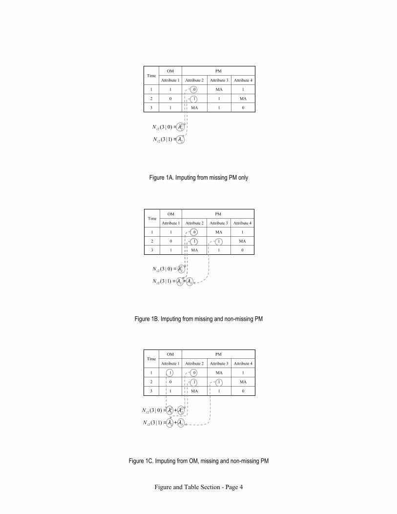
Figure and Table Section - Page 4
PMOM
1
1
MA
Attribute 3
0MA13
MA102
1011
Attribute 4Attribute 2Attribute 1Time
222 )0|3( λ=iN
22 )1|3( λ=iN
Figure 1A. Imputing from missing PM only
PMOM
1
1
MA
Attribute 3
0MA13
MA102
1011
Attribute 4Attribute 2Attribute 1Time
222 )0|3( λ=iN
322 )1|3( λλ +=iN
Figure 1B. Imputing from missing and non-missing PM
PMOM
1
1
MA
Attribute 3
0MA13
MA102
1011
Attribute 4Attribute 2Attribute 1Time
22
212 )0|3( λλ +=iN
322 )1|3( λλ +=iN
Figure 1C. Imputing from OM, missing and non-missing PM