a landscape-based ecological classification system for ... · a landscape-based ecological...
TRANSCRIPT

FISHERIES DIVISION
RESEARCH REPORT
STATE OF MICHIGANDEPARTMENT OF NATURAL RESOURCES
A Landscape-Based Ecological ClassificationSystem For River Valley Segments in Lower
Michigan (MI-VSEC Version 1.0)
Paul W. SeelbachMichael J. Wiley
Jennifer C. Kotanchikand
Matthew E. Baker
Number 2036 December 31, 1997

MICHIGAN DEPARTMENT OF NATURAL RESOURCESFISHERIES DIVISION
A LANDSCAPE-BASED ECOLOGICAL CLASSIFICATION SYSTEM FORRIVER VALLEY SEGMENTS IN LOWER MICHIGAN (MI-VSEC VERSION 1.0)
Paul W. SeelbachMichael J. Wiley
Jennifer C. Kotanchikand
Matthew E. Baker
The Michigan Department of Natural Resources, (MDNR) provides equal opportunities for employment and for access to Michigan’s natural resources. Stateand Federal laws prohibit discrimination on the basis of race, color, sex, national origin, religion, disability, age, marital status, height and weight. If you believethat you have been discriminated against in any program, activity or facility, please write the MDNR Equal Opportunity Office, P.O. Box 30028, Lansing,MI 48909, or the Michigan Department of Civil Rights, 1200 6th Avenue, Detroit, MI 48226, or the Office of Human Resources, U.S. Fish and Wildlife Service,Washington D.C. 20204.For more information about this publication or the American Disabilities Act (ADA), contact, Michigan Department of Natural Resources, Fisheries Division,Box 30446, Lansing, MI 48909, or call 517-373-1280.
Fisheries Research Report 2036December 31, 1997

1
Michigan Department of Natural Resources Fisheries Research Report No. 2036, 1997
A Landscape-Based Ecological Classification System for River Valley Segments in Lower Michigan (MI-VSEC Version 1.0)
Paul W. Seelbach
Institute for Fisheries Research Michigan Department of Natural Resources
212 Museums Annex Ann Arbor, Michigan 48109
Michael J. Wiley Jennifer C. Kotanchik and Matthew E. Baker
School of Natural Resources and Environment
The University of Michigan Ann Arbor, Michigan 48109
Abstract–Through ecological classification, researchers both (1) identify and (2) describenaturally-occurring, ecologically-distinct, spatial units from a holistic perspective. An ecologicalriver classification involves the identification of structurally homogeneous spatial units whichemerge along the channel network as a result of catchment processes interacting with localphysiographic features. Our observations of Michigan rivers suggest that the natural ecologicalunit, as defined by the spatial scales of riverine physical and biological processes, is most closelyapproximated by the physical channel unit termed the valley segment. Valley segments aregenerally quite large, and characterized by relative homogeneity in hydrologic, limnologic,channel morphology, and riparian dynamics. Valley segment characteristics often changesharply at stream junctions, slope breaks, and boundaries of local landforms. We followedseveral steps in developing an ecological classification for the rivers of lower Michigan. Step 1 –We first selected catchment size, hydrology, water chemistry, water temperature, valleycharacter, channel character, and fish assemblages as fundamental attributes to describeecological character of river valley segments. Steps 2-3 – Two experienced aquatic ecologistsworked together, interpreting map information on catchment and valley characteristics from aGIS, using their combined knowledge of ecological processes and interactions. We initiallyexamined several key maps to become familiar with the general landscape patterns of aparticular catchment; and to then identify initial valley segment units as defined by catchmentand valley characteristics, and fish assemblages. Boundary definition required the integration ofterrain features observed on several thematic maps (e.g., major stream network junctions, slopebreaks, boundaries of major physiographic units or land cover units; or changes in streamsinuousity and meander wavelength patterns, riparian wetlands, or valley shape), combined withknowledge of fish distributions. We next developed categorizations for each component attribute

2
and assigned category values for attributes to each segment unit. Assignments were based onmap-interpretation rules drawn from modeling, survey data, and field experiences. Step 4 – ourresults were stored as a map and a table in ArcView 3.0 format. In all, we partitioned andclassified the 19 largest river systems in lower Michigan. Summaries of the attributes assigned toover 270 river valley segments (covering mainstems and major tributaries) provided an initialdescription of the river resources of lower Michigan. Managers of lower Michigan rivers will beable to develop many of their thoughts and activities within this framework of ecological units.Development of this system is intended to be ongoing; with the extension of coverage to upperMichigan, the continued validation of attribute codings, and the addition of new attributes.
The utility of classification systems inecosystem management is widely accepted(Anonymous 1993). The tremendousdiversity of ecological systems makes itdifficult to generalize our managementexperiences or protocols from place to place.Ecological classification (defined asintegrating both physical and biologicalelements) provides a way of simplifying thiscomplexity, allowing generalization acrossrelatively homogeneous spatial units; andproviding a spatial framework for organizingdata, and extrapolating from site-specificmodels and information (Barnes et al. 1982;Rowe 1991; Hudson et al. 1992; Albert 1994;Maxwell et al. 1995). Ecologicalclassification also has a tremendouseducational value. It can provide acomprehensible summary of the complexarray of physical and biological processeswhich, over time, shape the natural worldaround us. Learning to recognize thelandscape as a mosaic of distinct ecologicalunits is valuable training for resourcemanagers, providing a short-hand for thinkingand communicating about the consequences ofcomplex ecological processes (Bailey et al.1978; Rowe 1984, 1991; Levin 1992).
Description of ecological classification Through ecological classification we both
(1) identify and (2) describe naturally-occurring, ecologically-distinct, spatial unitsfrom a holistic perspective. Ecologicalclassification differs from habitatclassification in the explicit use of biologicalcriteria, in addition to abiotic criteria, for
delineating unit boundaries. The ecologicalcharacter of each unit emerges as the unifiedexpression of its unique, abiotic (e.g., aspectsof climate and geology) and biological (e.g.,photosynthesis, respiration, and populationinteractions) processes (Spies and Barnes1985; Rowe and Barnes 1994). Theseecological units are observable places whereconstituent air, water, sediment, andorganisms co-occur as a distinct bio-physicalsystem (Rowe 1984, 1991; Rowe and Barnes1994).
Location and delineation of units is thekey, first step in ecological classification; thisoccurs “from above”, from a larger map-scale(Rowe 1984; Rowe and Barnes 1994). Theoperating hypothesis is that relatively-homogeneous ecological units exist; and canbe recognized in the spatial correspondence ofselected physical and biological traits, usingecological theory and field experience (Barneset al. 1982; Spies and Barnes 1985; Rowe1991; Rowe and Barnes 1994). Traits thatdrive numerous ecological processes are oftengiven extra weight; in terrestrial work forexample, physiography (land composition andform) is considered fundamental, as it isrelatively stable and helps shape local climate,soils, and vegetation patterns (Rowe 1984;Spies and Barnes 1985; Rowe 1991). Thedistributions of biota are also given specialweight as an important delimiting criteria,though they are inherently variable due totheir dependence on both ecological andhistorical processes. Biota can be importantdriving variables that help shape theecological unit, and their characteristicstypically integrate and express the overallecological signature of the unit (Rowe 1961;

3
Barnes et al. 1982). Ecological classificationsdescribe a unique place at a specific time(typically the present); therefore, culturally-derived landscape features (e.g., land usepatterns) are often included as ecologicalcriteria (Rowe 1989).
The second step involves describing theseunits by assigning them ecological attributes.Attributes are typically assigned based onobserved or predicted site-scale characteristics(Rowe 1984). Component attributes areusually expressed categorically and thisinformation is often used to formulate logicalgroupings of similar ecological units into unittypes (Spies and Barnes 1985; Rowe 1991).Davis and Henderson (1978), however,pointed out the value of retaining informationon as many component attributes as possible,as this provides the most flexible informationset.
Ecological classification of river units Early river classifications included
ecological, longitudinal zonation schemes thattied distinctive community composition to keyphysical variables such as temperature,substrate and network position; and systemsbuilt on distributions of selected biota (seereview by Hudson et al. 1992). Morerecently, greater emphasis has been placed ondescribing physical channel units at variousscales (Frissell et al. 1986; Hawkins et al.1993; Rosgen 1994; Maxwell et al. 1995) toprovide a physical habitat templet fordescription of the structure and operation ofstream communities (Frissell et al. 1986).This parallels the concept of the geocoenoseused by forest ecologists in Europe (Kimmins1987; Rowe and Barnes 1994).
Our interest in a more ecologicallycomprehensive system can be illustrated withan example. Imagine two tributaries to LakeMichigan that are identical in catchment andvalley characteristics (physical habitattemplate). However, only one has a barrierdam within a lower reach that excludesmigratory fishes from Lake Michigan (e.g.,Pacific salmon). Exclusion of these fish willarguably alter fish community structure, food
webs, nutrient cycles, and toxic chemicalconcentrations in the dammed stream—thusthe presence or absence of fishes help define astream’s fundamental ecological character.
Terrestrial ecologists have generallytreated the spatial organization of thelandscape as a hierarchically-nested mosaic ofecological units (Bailey et al. 1978; Albert etal 1986; Barnes et al. 1982; Rowe 1991).Sites (plots) represent basic sampling units butthe smallest ecological unit is the land typeassociation (= geo-ecosystem =biogeocoenose; Rowe 1961, 1969; Rowe andBarnes 1994; Kimmins 1987), which has arelatively homogenous floral community, andconsistent edaphic and micro-climaticfeatures. Regional ecosystems (sensu Albertet al. 1986; Albert 1994) represent units nearerthe top of the hierarchy and incorporate largeregions (100’s to 1000’s of square miles) ofsimilar climate and physiography. A parallelhierarchy of riverine units has been suggested:ie. sites, valley segments, and watersheds(Chamberlin 1984; Frissell et al. 1986;Maxwell et al. 1995).
Ecological classification of river systemsat a scale useful for management has beenproposed (Hudson et al. 1992; Maxwell et al.1995) but seldom implemented across anylarge region. An ecological river classificationinvolves the identification of structurally-homogenous spatial units within the river(analogous to the terrestrial ecologists’ecosystem type but with similar aquaticchemistry, biota, temperature, hydraulics, andriparian structure), which emerge along thechannel network as a result of catchment-scaleecological processes interacting with localphysiographic features.
Ecological river units – valley segments River systems are typically viewed as
composed of many smaller, distinct ecologicalunits (Balon and Stewart 1983; Chamberlin1984; Naiman et al. 1988; Halliwell 1989;Hudson et al. 1992; Bayley and Li 1992;Maxwell et al. 1995). One can identify riversegments having distinctive, relativelyhomogeneous (or ordered patterns of)

4
hydrology, hydraulics, chemistry, temperatureregime, channel morphology, channel habitat,sediment budget, disturbance regime, andcommunity structure. Boundaries betweenthese units are relatively distinct (whenviewed at the appropriate scale), because:
• The abrupt junctures of unrelatedhydrologic systems (e.g., the confluence ofstreams draining independent catchments)can result in marked changes in ecosystemproperties associated with hydrology. Forexample, discharge itself can increasedramatically, with rapid responses insensitive thermal and hydraulic regimes(Statzner and Higler 1985; Frissell et al.1986). Additionally, the addition of uniquewaters can alter chemical, thermal, andmaterial-load conditions (Minshall et al.1985).
• The linear river passes across a mosaic oflandscape types with abrupt boundaries(Naiman et al. 1988; Maxwell et al. 1995;Bryce and Clarke 1996; Corner et al. 1997).Local geologic features influence immediateslopes (and thus hydraulics), channel crosssections, meandering patterns, developmentof pools and riffles, substrates, andgroundwater inputs (temperatures); and canact as mid-river base-level controls onupriver grade (Statzner and Higler 1985;Frissell et al. 1986; Cupp 1989; Rosgen1994; Bryce and Clarke 1996). Localgeomorphologies (e.g., plains, hills andmountains, or glacial valleys) also affectchannel forms, including floodplainstructures (Minshall et al. 1985; Frissell etal. 1986; Cupp 1989; Rosgen 1994; Baker1995). Local vegetation influences shadingof, and carbon inputs to, the stream (Frissellet al. 1986).
• The (unpredictable) presence of mid-riverlakes and impoundments can likewise act asbase-level controls on upriver grades(Statzner and Higler 1985), and have strongeffects on downstream chemical, thermal,and material regimes (Ward and Stanford1983; Minshall et al. 1985; Frissell et al.1986).
The whole river system, then, is abranched, linear mosaic of these ecologicalunits; patterned both by longitudinal(catchment-derived) factors (such asaccumulating discharge; Minshall et al. 1985)and by location-specific factors (such asgeology and geomorphology; Statzner andHigler 1985; Frissell et al. 1986; Cupp 1989;Hudson et al. 1992; Bryce and Clarke 1996).
Our observations of Michigan riverssuggest that the natural ecological unit, asdefined by the spatial scales of riverinephysical and biological processes, is mostclosely approximated by the physical channelunit termed the valley segment. Valleysegments are variable in length, but aregenerally quite large (perhaps 3-60 km [2-40mi]). A segment is characterized by relativehomogeneity in hydrologic, limnologic,channel morphology, and riparian dynamics(Frissell et al. 1986; Cupp 1989; Hudson et al.1992; Rosgen 1994; Maxwell et al. 1995).Valley segment characteristics often changesharply at stream junctions, slope breaks, andboundaries of local landforms. Segmentboundaries can be interpreted from large-scalemaps and segment attributes can be easilyfield-verified.
The valley segment scale is attractive forthe study of river ecological units for severalreasons:
• It is close to the scale at which rivers reactto heterogeneity in the landscape byforming channel networks; and respondingto local slopes, geologic materials, and landuses (Maxwell et al. 1995; Bryce andClarke 1996). Each segment of the riverbisects a fairly homogeneous landscape unit(e.g., Corner et al.’s [1997] LandtypeAssociations). Segments also describerelatively persistent features of channel andriparian habitats (on the order of 102-103
years; Hudson et al. 1992; Baker 1995).
• The valley segment scale is similar to thatat which fish (and other aquatic organisms)operate (Hawkes 1975; Maxwell et al.1995). One, or several adjacent, segmentsare large enough to likely contain themultiple habitats required by stream fishesduring their life cycle (Schlosser 1991). It

5
follows that several physically-definedvalley segments might sometimes beincorporated as one ecological unit. It isclear that stream fishes are extremelymobile, especially among seasonal habitats(Gowan et al. 1994, Bayley and Li 1992);so smaller units such as reaches or channelunits are inadequate to encompasspopulation dynamics.
• Though fairly homogenous, segments alsohave internal organization represented bysome predictable series of smaller-scalereach units (e.g., alternating stretches ofrelatively consistent slopes within thesegment) and further-nested channelhabitats (e.g., pools, riffles, substrates) thatare used by organisms during specific lifestages and seasons (Rowe 1969; Frissell etal. 1986; Hudson et al. 1992; Hawkins et al.1993; Rosgen 1994). Thus segmentattributes can include the description ofpatterns in local habitat structure andprovide a framework for smaller-scaleclassifications where desired.
• The valley segment is probably the smallestriver unit that can be interpreted from large-scale maps and analyzed across largegeographic areas (states or regions; Frissellet al. 1986; Maxwell et al. 1995). Theprimary landscape features of interest (e.g.,river networks, slopes, geologic materials,and land uses) are readily observed on mapsof 1:100,000 or even 1:500,000 scales.
• Information at this scale is relevant formanagement and planning, since it is thescale at which important physical andbiological processes operate. Individualsegments have predictable ecological traits,allowing the development of localmanagement goals and strategies. Andsegments are few enough that informationcan be easily compiled for regionalanalyses.
Developing an ecological classification forMichigan rivers
We used the following 6 steps in thedevelopment of our classification (modifiedfrom the more general steps provided byDavis and Henderson 1978).
• Step 1 is the selection of key attributes foridentifying ecological units. Variablesselected for river classification should be(1) fairly stable in time; (2) easilyquantifiable; (3) representative of eithercatchment-scale hydrologic, or local-scalegeomorphic, processes; and (4) determinateof smaller-scale habitat and biotic processes(Dunne and Leopold 1978; Dewberry 1980;Lotspeich and Platts 1982; Frissell et al.1986; Cupp 1989; Poff and Ward 1989;Hudson et al. 1992; Newsom 1995; Rosgen1994; Baker 1995; Maxwell et al. 1995;Vannote et al. 1980). Oft-suggestedphysical variables that drive streamecosystems are stream size, hydrology,channel slope, temperature, and substratesize. Biotic groups used in classificationsinclude fishes, macro-invertebrates, andmacrophytes.
• Step 2 involves both selection of key mapsthat index attributes and definition ofmapping rules for delineating unitboundaries. River segment boundaries aretypically associated with stream junctions,major slope breaks, boundaries of locallandscape ecosystems, and changes in fishassemblage structure.
• Step 3 is the development of classificationcategories for each attribute. Categoriesshould be defined so as to reflect both theexisting range of values for that attributeand significant changes in ecosystem unitcharacter.
• Step 4 is the definition of rules forassigning attribute classes to each unit.Assignments are either based on existingsite-level data, or based on knownqualitative or quantitative relationshipsbetween map information and selectedattribute classes (e.g., Hakanson 1996;Ladle and Westlake 1995).

6
• Step 5 is the development of acomputerized information system forstorage, retrieval, and display ofinformation on ecosystem boundaries andattributes. In the past, multiple-attributedata were often integrated to describeecosystem “types” (typically on papermaps) and useful information was lost.Today’s Geographic Information System(GIS) technologies offer powerful newopportunities for development, storage,query, analyses, and display of both spatialand tabular data. Thus, all componentattribute information can be retained in aflexible system that can be responsive to theneeds of a variety of users (Davis andHenderson 1978; Hudson et al. 1992).
• Step 6 is the grouping of units by selectedattributes to create any one of a number ofpossible classifications. Again, thisflexibility is made possible by advances incomputer technology. Multiple attributescan be selected, perhaps weighted, andintegrated into a holistic ecologicalclassification. Such a grouping wouldprovide a sound ecological stratificationuseful for a wide variety of managementneeds, especially those stemming from adesire for holistic ecosystem management.Other, more narrow thematic classifications(e.g., water temperature or valley character)could also be created in response to specificneeds.
Despite only mild variation in climate andelevation across lower Michigan, manysuccessive glaciations have created anexceptionally-varied ecological landscape.Lower Michigan is a mosaic of glaciallakeplains, outwash plains, moraines, and tillsof varying depths and textures (includingsome of the deepest deposits of glacialoutwash sands and gravels in North America;Dewberry 1980; Farrand and Eschman 1974;Farrand and Bell 1984; Albert et al. 1986).This peninsula is laced with old glacial-fluvialchannels and bedrock protrudes in a fewlocations. River catchment hydrology; therouting of water among evapotranspiration,groundwater, and overland flow pathways;
therefore varies tremendously across systems(baseflows range from near zero to some ofthe highest in North America; Hendricksonand Doonan 1972; Dewberry 1980; Holtschlagand Crosky 1984; Poff and Ward 1989;Rheaume 1991; Berry 1992; Richards 1990).Additionally, a surprising variety of localvalley characteristics and constraints areencountered as stream channels move acrossspecific glacial terrains, and in and out of oldglacial-fluvial channels (Dewberry 1980;Baker 1995). In the upper Midwest,distributions of stream biota have been shownto relate to patterns in catchment and localsurficial geology and hydrology (Threinen andPoff 1963; Hendrickson and Doonan 1972;Dewberry 1980; Strayer 1983; Bowlby andRoff 1986; Meisner et al. 1988; Wiley et al.1997; Zorn et al. 1997).
The only existing classification ofMichigan rivers and streams was developed bythe Michigan Department of NaturalResources, Fisheries Division in 1967(Anonymous 1981). This system was notbased on habitat attributes, but essentially onthe distribution and abundance of game fishes(some attributes of stream size, ripariandevelopment, and potential for boating wereincorporated). Attributes were assigned basedon field experiences of state biologists andconservation officers, complimenting surveydata where it existed. This classification wasprobably quite accurate regarding thedistribution of waters containing trout--themost well-studied fishes--but less informativeregarding other waters. No hierarchical,habitat-based or ecological classificationexists for Michigan rivers, or for rivers insimilar glaciated and partly-agriculturalterrains. Most of the primary literature onstream classification has instead beendeveloped in forested, mountainous areas(e.g., Frissell et al. 1986); where variablesdriving stream ecological characteristics arelikely quite different than in Michigan.
As one component of the larger, MichiganRivers Inventory (MRI) Project (see Seelbachand Wiley 1997), we endeavored to build anecological classification system for the riversof lower Michigan. Our specific studyobjectives were:

7
• To identify ecologically-distinct river valleysegments within the rivers of lowerMichigan.
• To develop landscape-based classificationsfor selected ecological attributesrepresenting aspects of catchmenthydrology, local valley constraints, andrepresentative biota.
• Through the interpretation of maps, toassign attributes for each of these traits toeach valley segment.
• To develop a digital map and databaseinformation system (GIS) for retrieving andviewing the classification data andsupporting map images.
• To provide an initial ecological typing ofsegments.
Approach and methods
Selection of key attributes for identifyingecological units
We selected catchment size, hydrology,water chemistry, water temperature, valleycharacter, channel character, and fishassemblages as fundamental attributes todescribe the ecological character of rivervalley segments. Stream size indexesimportant longitudinal gradients in riverhabitats and has long been recognized as aprimary classification variable (Hawkes 1975;Vannote et al. 1980). Hydrology, waterchemistry, and water temperature integratecomplex catchment processes and are alsoimportant proximal variables shaping localbiology. Valley character reflects localphysiography and constrains channeldevelopment. High in the trophic web, fishesare good integrators and express the conditionof their complex environments (Fausch et al.1990).
Selection of key maps
The general ecological character of each
segment was interpreted by searching maps
for “terrain features that control the intensityof key factors” (Rowe 1991). We focused onkey map characters identified in prior MRImodeling efforts as important catchment- andlocal-scale drivers of each attribute (Table 1).Terrestrial classifiers have noted thesignificance of physiography as a keyecological driver (Rowe 1984; 1991; Spiesand Barnes 1985). We also paid particularattention to the catchment- and local-scalephysiography that influence hydrology, whichis central to river ecology.
Both classification steps – identificationof units and assignment of attributes – weredone “from above”, by the interpretation ofdigital maps displayed in a GIS environment.We were able to use maps to assign attributesby predicting site-scale attributes fromlandscape-site models developed within theMRI project. Key map themes used aredescribed in Table 2. Two experiencedaquatic ecologists worked together,interpreting map information on catchmentand valley characteristics, using theircombined knowledge of ecological processesand interactions. The shared experiences of,and discussion between, mappers was acritical component of this process (asemphasized by Spies and Barnes 1985; Rowe1991). These ecologists studied a variety ofmaps compiled by the MRI project, usingArcView (Version 3.0; ESRI, Inc.) softwarerunning on either a SUN (UNIX) computer ora PC (Windows 95 or Windows NT) computerserving as a terminal to the SUN machine.This was an extremely flexible and powerfulanalytical environment; at the users’discretion, multiple map layers could be easilyoverlain and the viewing scale easily changed.
Mapping rules for delineating unit boundaries Step 1. Initial identification of valley
segments and segment boundaries using keymap features.–We initially examined severalkey maps to become familiar with the generallandscape patterns of a particular catchment;and to then identify initial core river segmentsas defined by segment boundaries. Definitionof an ecological boundary first required the

8
integration of terrain features observed onseveral thematic maps (sensu. Barnes et al.1982; Rowe 1991): major stream networkjunctions, slope breaks, boundaries of majorphysiographic units or land cover units; orchanges in stream sinuousity and meanderwavelength patterns, local groundwater inputs,riparian wetlands, or valley shape (bottomwidth and side slope). Specifically:
◊ Elevation and wetland maps were examinedfor changes along the river’s course invalley channel slopes and side slopes,valley width and origin (glacial or alluvial),and floodplain wetlands (Figure 1).
◊ Maps of surficial geology and predictedgroundwater velocity were examined forchanges occurring between major glacialformations (e.g., lakeplains, outwash plains,till plains, end moraines) and among drifttextures (fine, medium, coarse); and toidentify the positions of glacial-fluvialchannels (bands of outwash in definitivevalleys), and local or regional groundwatersources.
◊ Maps of stream networks, lakes, andwetlands were examined for locations ofmajor network junctions, the break between“headwaters” and the river (largely ajudgement call based on stream size;headwater tributaries generally hadcatchments < about 400 km2), majortributaries (given segment status based onstream size), large lakes, and wetlands; andfor changes in channel sinuosity (Figure 2).
◊ Land cover maps were examined forchanges between major zones (e.g. betweenforested and agricultural areas).
Ecological changes suggested byphysically-derived boundaries wereinvestigated by looking for correspondingchanges in fish assemblages (Balon andStewart 1983; Spies and Barnes 1985; Rowe1991).
◊ We cross-checked potential abruptphysical boundaries against informationon fish distributions derived from sitedata, field experience, and landscape-
based predictive models (Zorn et al.1997).
◊ We also kept in mind that, despitepotential small-scale physical variation insome areas, ecological segments needed toremain fairly large, relevant to the scale ofuse by fish populations (Hawkes 1975;Maxwell et al. 1995).
Frissell et al. (1986) recommended thatlakes be treated as individual valley segments,in essence as ecological units. We agree butdid not address the thousands of lakes andreservoirs found in lower Michigan in thisinitial effort. We expect to include a limitednumber of the larger lakes and impoundmentsas segments in future versions.
Step 2. Finalize segment breaks.–We thendetermined the final segment boundaries byapplying the following system of priorities:
I. Major junctions in the hydrologic network(for mainstem and major tributarysegments).
II. Corresponding breaks determined fromslope, channel constraints, and geologicboundaries.
III. Changes in groundwater source, oftencorresponding with II.
IV. Abrupt changes in major land coverpatterns.
Step 3. Review segment breaks.–Duringthe process of assigning ecological attributesto segments (see below), we double-checkedthat at least one coded ecological trait changedbetween adjoining segments (typically thiswould also include a change in fishassemblage). If this criteria was not met, wecombined the segments in question.
Classification categories and mapping-assignment rules for ecological attributes
Basin and watershed names.–The GreatLake basin and major watershed system towhich each segment belonged were identified(Table 3).

9
Unique segment ID number and series ofposition numbers.–Each segment was given aunique identification (ID) number, as well as aseries of numbers that contained informationabout its position in the river net. The firstnumber in this series represented themainstem segment ID number, beginning with“1” at the river mouth and progressing up themainstem as “2, 3, etc.” The upstream-mostsegment stopped short of the headwaters.
The next set of 2 numbers in the seriesrepresented the net position of the majortributary segments. The first numberdescribed the position of juncture with themainstem segment; numbering was “1, 2, etc.”working upstream along the particularmainstem segment. For example thedownstream-most large stream joining thedownstream-most mainstem segment wouldbe “1 1 _”; the next-upstream large tributarywould be “1 2 _”; and so forth. The secondnumber described position within the majortributary itself; numbering was “1, 2, etc.”working upstream on the tributary. Forexample a major tributary that has 3 segmentsand joins the lower mainstem segment wascoded “1 1 1, 1 1 2, and 1 1 3”.
Larger tributaries to major tributaries werecoded using the same logical sequence insubsequent sets of 2 numbers. For examplethe second-upstream segment of thedownstream-most major tributary to thedownstream-most major tributary to thelowest mainstem segment was coded “1 1 1 12”.
Headwaters and tributaries that flowed toa common segment and that sharedfundamental ecological properties were codedas a group. These were given a unique groupcode, numbered as “1,2, etc.” representingvarious groups in no particular upstream-downstream order. An example set of codes isshown in Figure 3.
Segment catchment size.–Segmentcatchment size, an index of stream size, wasindexed as the link number determined at thedownstream end of each segment. The linknumber is the sum of the first-order streams(streams with no upstream branches) in theupslope catchment (Osborne and Wiley 1992).We interpreted link numbers from a stream
network map of Michigan built from 1:24,000USGS maps (Michigan Resource InformationSystem, Michigan Department of NaturalResources, Real Estate Division, Lansing).The interpretation of first-order streams onthis map is slightly different than on theUSGS Digital Line Graph (DLG) maps thatwe used throughout the rest of the project--thisdiscrepancy should be resolved in futurerevisions.
Segment position in the river net.–Network position indicates the proximity of asegment to potential downstream sourcepopulations, and has been shown to influencefish community composition (indexed by d-link number; Osborne and Wiley 1992;Osborne et al. 1993). Some information on theposition of a segment in the river net (e.g.,high in the headwaters vs. down towards themouth) was provided in the series of positionnumbers. A more specific measure of positionrelative to river size was measured as the d-link number (Osborne and Wiley 1992) at thedownstream node of each segment. The d-link number is the link number at the next-downstream network juncture (we excludedjunctures with tributaries with link numberssmaller than 10% of the exisitng link number).Figure 4 shows an example of link and d-linknumbers for a segment.
Connection to the Great Lakes.–Similar tonetwork position, connection to the GreatLakes indicates potential faunal sourcesinfluencing assemblage structure. Werecorded whether a segment was openlyconnected to the Great Lakes or cut off by abarrier dam, as codes 1 and 2, respectively.
Hydrology codes.–We coded thehydrology for each segment as 1 of 9 generaldischarge patterns observed in Michiganhydrologic data (MRI, unpublished). Adischarge pattern was inferred by examiningthe composition of catchment topography,surficial geology, and land cover. Thesepatterns were considered to be size-independent and discharges were consideredin terms of yields (cfs/km2 of catchment). [inthis and following ecological codings, we alsoconsidered the ultimate sequence of codings
10
with up- and down-stream neighbor segments--codings should change along the system in areasonable pattern/story]. The 6 most-commonpatterns represent a continuous seriesillustrating tradeoffs between groundwater andrunoff sources (Figure 5). These were dividedinto a group of 2 primarily groundwater-driven streams and a group of 4 primarilyrunoff-driven streams. Each group was furtherbroken down based on baseflow and peakflowyields as follows:
• G1 – groundwater-driven, with very highbaseflow and low peakflow. Catchmentcomposition is fairly high-relief, ice-contact hills and coarse-textured endmoraines surrounding extensive outwashplains (Figures 6a and 6b). Examplesinclude the Au Sable, Boardman, LittleManistee, Manistee, and Platte rivers.
• G2 – groundwater-driven, with highbaseflow and moderate peakflow.Catchment composition is relatively high-relief coarse end moraines draining ontooutwash plains, often with some coarse tillplains, medium-textured end moraines, ormedium till plains present. Examplesinclude the Black and Sturgeon (Cheboygansystem), Pine (Manistee), Rifle, PereMarquette, and Paw Paw rivers.
• R1 – runoff-driven, with fair baseflow andmoderate peakflow. Catchmentcomposition is a mixture of moderate-reliefcoarse end moraines, coarse till plains, andoutwash plains. Examples include theMuskegon, Thunder Bay, and Kalamazoorivers.
• R2 – runoff-driven, with moderate baseflowand fair peakflow. Catchment compositionis a mixture of low-relief coarse andmedium end moraines, and medium tillplains, with some outwash plains (Figures7a and 7b). Examples include the Grand,Huron, and St. Joseph rivers.
• R3 – runoff-driven, with low baseflow andhigh peakflow. Catchment composition isprimarily medium and fine-textured tillplains, and lacustrine plains, with somelow-relief medium and fine end moraines
present. Examples include the Cass,Shiawassee, and Maple rivers.
• R4 – runoff-driven, with very low baseflowand very high peakflow. Catchmentcomposition is primarily lacustrine plains.Examples include the Kawkawlin,Macatawa, and Pigeon rivers.
Three somewhat unusual flow patterns
were also identified (Figure 8):
• GS – groundwater-driven, with super-highbaseflow and moderate peakflow.Catchment composition is similar to G2streams, but groundwater is gained fromadjacent aquifers (determined from specifichydrologic records, not from maps).Examples include the Jordan River.
• GW – groundwater-driven, influenced byextensive wetlands, with moderate baseflowand very low peakflow. Catchmentcomposition is similar to either G1 or G2streams, but with extensive wetlandcoverage resulting in highevapotransporative losses. Examplesinclude the South Branch Au Sable andClam rivers.
• RW – runoff-driven, influenced byextensive wetlands, with very low baseflowand very low peakflow. Catchmentcomposition is generally similar to S3 or S4streams, but with extensive wetlandcoverage and high evapotransporativelosses. We have no gaged examples of thistype.
Water chemistry codes.–Segment waterchemistry was considered to be a product ofcatchment hydrology and land cover, and wasdetermined from hydrology codes andinterpretation of surficial geology, soils, andland cover maps (based on relationshipsdeveloped by Kleiman 1995). Chemistry wasfirst categorized as either oligotrophic (typicalvalues: SRP < 15 ppb, NO
3+NO
2 < 100 ppb),
mesotrophic (typical values: SRP 15-30 ppb,NO
3+NO
2 100-700 ppb), or eutrophic (Figures
9-12). These categories were further dividedas follows; based on effects of upstream lakesand wetlands, and land cover intensity:

11
• OS – oligotrophic, with low nutrients andlow alkalinity (soft water). Flow pattern istypically S2 or S3, due to catchmentsurficial geology dominated by shallowdrifts overlying bedrock or peaty soils.Catchment land cover includes substantialwetlands. Possibly an upstreamombrotrophic lake or wetland.
• OH – oligotrophic, with low nutrients andhigh alkalinity (hard water). Flow pattern isG1, G2, GS, or GW. Catchment land coveris mostly forested. Possibly an upstreamminerotrophic lake, springs, or wetlands.
• M – mesotrophic, with moderate nutrients.Flow pattern is G1, G2, S1, or SW.Catchment land cover is a mixture of forestand light agriculture, with some wetlands.
• MW – mesotrophic, influenced byextensive wetlands, with moderatephosphorus and low nitrates. Flow patternis G1, G2, or S1. Catchment land cover is amixture of forest, light agriculture, andextensive wetlands.
• E1 – eutrophic, with moderate to highnutrients. Flow pattern is S2, S3, or S4.Catchment land cover is mixed forest, lightresidential, and light agriculture.
• E2 – eutrophic, with high nutrients. Flowpattern is S2, S3, or S4. Catchment landcover is agriculture and suburban.
• EG – eutrophic groundwater-driven stream,with high nutrients in the groundwater.Flow pattern is G1, G2, GS or S1.Groundwater contamination is fromagriculture on permeable soils (e.g.,orchards).
• EU – eutrophic stream in an urban area,with high nutrients and pollutants. It couldhave any flow pattern. Its catchment orlocal area is heavily urbanized.
Water temperature codes.–Patterns inboth summer temperature means and diurnalfluctuations were considered to be drivenprimarily by catchment hydrology and size,modified by upstream lake and shading effects(Figures 13-14).
Our codes described a matrix of 3categories for July weekly mean temperaturesby 3 categories for July weekly temperaturevariation (Figure 15; Wehrly et al. 1997).Matrix divisions were based on observedsummer temperature boundaries in relation tothe distributions of coldwater (brown trout)and warmwater (smallmouth bass) gamefishes.
July temperature codes were assignedbased primarily on hydrology codes andvisually-estimated relative catchment size,using the relationships shown in Figures 13-14. Codes were modified according topotential impacts of upstream land coverpatterns, presence of upstream lakes, andlatitude (air temperature). Some codes couldbe attained through several alternativecombinations of key variables. We alsoconsidered the downstream sequence of codesamong neighboring segments. Some commonsequences in temperature codings are shownin Figure 16. Codes were as follows:
• CL – cold mean and low diurnal variation.Catchment size is very small to small, witha very large groundwater source andextensive shading.
• CM – cold mean and moderate diurnalvariation. Catchment size is small tomedium, with a large groundwater source.Shading important on smaller streams.
• CH – cold mean and high diurnal variation.We have no examples of this uncommontype.
• KL – cool mean and low diurnal variation.Catchment size is large with a moderate tolarge groundwater source; or medium-sizedwith a medium groundwater source andsubstantial shading.
• KM – cool mean and moderate diurnalvariation. Catchment size is medium with alarge groundwater source; or small with amoderate groundwater source.
• KH – cool mean and high diurnal variation.Catchment size is small with littlegroundwater input.

12
• WL – warm mean and low diurnalvariation. Catchment size is very large,with either small groundwater or moderategroundwater inputs.
• WM – warm mean and moderate diurnalvariation. Catchment size is medium, withsmall or moderate groundwater.
• WH – warm mean and high diurnalvariation. Catchment size is medium withlittle groundwater input.
Valley slope codes.–Valley slope was
interpreted from elevation and topographymaps as 1 of 3 broad categories.
• VL – very low valley slope, roughly < 4ft/mi (< 0.00076 %). Typical of fine tillplains and lacustrine plains, with abundantwetlands. Channel habitats include runsand pools.
• L – low valley slope, roughly 4-10 ft/mi(0.00076 - 0.0019 %). Typical of outwashplains, medium and coarse till plains, andsome medium and coarse end moraines, andsome ice-contact hills. Some riffle habitatspresent.
• M – moderate valley slope, roughly > 10ft/mi (> 0.0019 %). Typical of many coarseend moraines and ice-contact hills. Channelhabitats are typically alternating riffle-poolsequences.
Valley character codes.–Valley character
codes described the degree of channelconfinement, either by coarse-texturedmorainic features, old glacial-fluvial channelwalls, or deeply-incised alluvial channel walls.Valley character was descriptive of constraintson the stream channel and local parentsubstrates. It was interpreted from localelevation, topography, surficial geologypatterns, and wetland patterns as one of the 8categories described below. A glacial-fluvialvalley was created thousands of years ago by avery large, glacial meltwater river. Analluvial valley has been carved by the currentriver.
• GU – glacial and unconfined. Channelflows unconfined within a relatively broadglacial-fluvial valley.
• GC – glacial and confined. Channel isconfined by a relatively narrow glacial-fluvial valley.
• GI – glacial and incised. Channel isconfined by alluvial incision in a broadglacial-fluvial valley.
• GS – glacial and sporadically confined.Channel is sporadically-confined bymorainic features within a broad glacial-fluvial valley.
• AU – alluvial and unconfined. Channel isunconfined as it cuts across broad till,outwash, or lacustrine plains.
• AC – alluvial and confined. Channel isconfined in an alluvial valley.
• AS – alluvial and sporadically confined.Channel is sporadically-confined bymorainic features within broad till, outwash,or lacustrine plains.
• AA – alluvial with alternating confinement.Channel cuts alternatively across morainicfeatures and plains.
Channel character codes.–We notedwhether a channel was single and meandering,multiple (braided or anastomozing), orchannelized with the codes listed below.Channel character was interpreted from mapsof channel networks.
• S – single, meandering channel.
• B – braided or anastomozing, multiple channels.
• D – ditched or channelized channel.
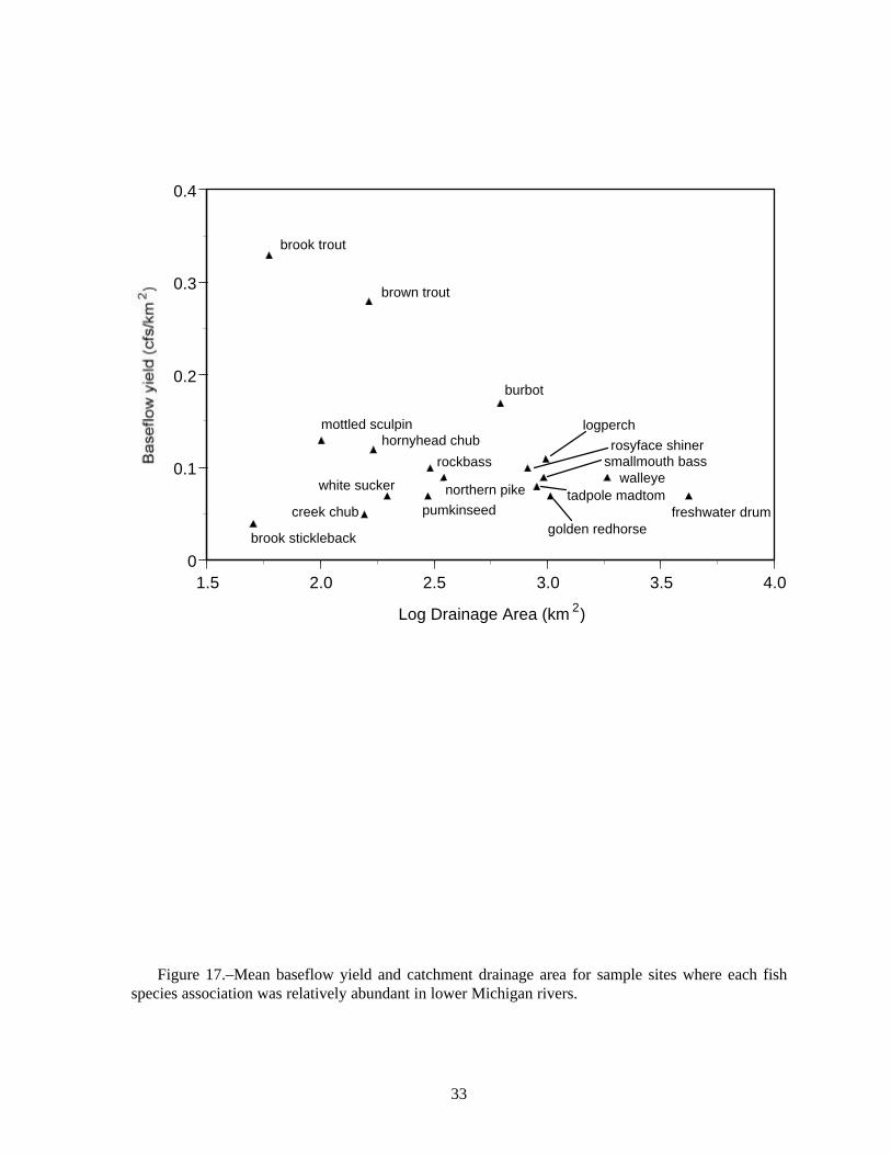
Fish species association codes.–We codedthe fish species associations most likely tooccur at each segment. Fish speciesassociations were determined by Zorn et al.(1997) through a hierarchical cluster analysisusing relative abundance data for the 69 mostcommon riverine fish species, at 225 sitescontained in the Michigan Rivers Inventorydatabase (Seelbach and Wiley 1997; Table 4).

13
Each cluster is represented by the name of adiagnostic species.
Mean baseflow yield and catchmentdrainage area were calculated for sites whereeach species association was relativelyabundant (>0.25 as standardized z-scores;Figure 17; Zorn et al. 1997). Likely speciesassociations were determined for eachsegment by interpreting hydrologic patternsand catchment size from the GIS maps, takingadditional map variables (land cover patterns,river net position, and connectivity) and fieldexperience into consideration.
Initial validation of fish-association codings
We did some initial validation of the fishassociation codings. We focused on these, asfishes are considered to be a response variablethat integrates the other, physical habitatcodings. We checked our codings againststream survey records (Michigan Departmentof Natural Resources, Stream CollectionRecords, Ann Arbor). And we interviewedMichigan Department of Natural ResourcesDistrict Fisheries Biologists regarding theirfield experiences with fish distributions andgeneral river segment identifications. Often,field data and experiences confirmed our fishcodings and our overall interpretation of thesegment’s ecology. When fish data andexperiences did not match our originalcodings, we did one of the following: (1) Ifcodings were marginal between twocategories, we changed the fish codes to matchthe data; (2) If codings and data were verydifferent at a particular site, we assumed thatthe current fishes may be reflecting sitemodifications not apparent from our large-scale maps and used the physically-basedcodings as representing potential fishes; or (3)If the codings and the data were mismatchedat a series of sites, we tried to learn from thispattern and revise our coding proceduresaccordingly.
GIS and database Methods
Classification map and table data werestored in ArcView, Version 3.0 (ESRI, Inc.)formats, on a Unix-based Sun computer. Thedownstream break of each segment wasmarked and identified as a point in anArcView shapefile. Attribute codings wereentered into a data table (format “.dbf”) wherecodings were fields associated with eachsegment (record). When joined (in ArcView)with the shapefile’s associated data table,codings associated with each record werelinked to the mapped points and were thenaccessible through either the GIS mapenvironment or through the database queryfunctions of ArcView. Attribute codings werealso linked to mapped segment-bufferpolygons (thicker stream lines), which weredeveloped by modifying the stream networkmap in ArcView.
Ecological typing
The attribute table provides a basis for thedevelopment of a variety of ecologicalsegment types, potentially varying in theiremphasis and complexity. As an initialexample, we did a simple cross-tabulation of 3key attributes that index important ecologicaltraits: hydrology, water temperature (thisbrought in some information on river size andwas a good index of fish composition), andvalley confinement (Dewberry 1980; Halliwell1989). Our goal was to look for segmentattribute sets that repeated across lowerMichigan (Speis and Barnes 1985).
Results
Description of segments and attributes
We partitioned and classified the 19largest river systems in lower Michigan,calling this initial effort MI-VSEC (MichiganValley Segment Ecological Classification)Version 1.0. A river system was defined ashaving an outlet to the Great Lakes, with theexception of the large Saginaw River system,

14
which we arbitrarily broke into 3 subsystems(Tittabawassee, Shiawassee, and Cass rivers)that meet to form the Saginaw River propernot far from Saginaw Bay (Lake Huron). Weidentified and described 271 river valleysegments that covered river mainstems andmajor tributaries. (We also did initialdescriptions for 504 sets of minor tributariesand headwaters of these rivers, but these arenot described in this report). The number ofmainstem segments per river was typically 4-5, ranging from 3 to 7. The number of majortributary segments per river system variedwith basin size but was typically 1-12, withsome as high as 17-27. Segments averaged 38km in length and ranged from 3 km to 320 kmin length; segments were generally longer inlarger rivers.
Summaries of the assigned attributesprovide an initial description of the riverresources of the Lower Peninsula. Due torelatively short drainages to the Great Lakes,river size is generally small to moderate(Figure 18). Many smaller streams are linkedto larger downstream waters (Figure 18); butdespite their proximity, only 29% of segmentsare today directly connected to the GreatLakes (due to numerous dams). LowerMichigan’s porous surficial deposits provideextensive groundwater inputs to almost 1/3 ofsegments and moderate groundwater inputs toan additional 1/3 of segments (Figure 19).Some segments show relatively low nutrientlevels, reflecting catchments composed largelyof sands and gravels; but most havesubstantial nutrients, due to more loamy soilsand human influences (Figure 20). Mostsegments have low channel gradients and rununconfined across outwash, till, and lakeplains(Figures 21-22). Segments with moderategradients and confined channels–these containrocky substrates, distinct riffle-poolsequences, and perhaps rapids–are relativelyrare. Although we have traditionallycategorized Michigan streams as eithercoldwater or warmwater (Anonymous 1981),most segments had cool means and (regardlessof mean) most segments also had moderatedaily fluxes (Figure 23). These intermediatethermal conditions allow many segments tohold a variety of fishes (Figure 24), though
they are not necessarily ideal for thermally-specialized game fishes such as trout.
Examples of ArcView maps and tables
Our results were stored as a map and atable in ArcView 3.0 format, and are availableupon request from the Michigan Departmentof Natural Resources, Institute for FisheriesResearch, 212 Museums Annex, Ann Arbor,MI (telephone 313-663-3554; web addresshttp/www.dnr.state.mi.us/www/ifr/ifrlibra/ifrlibra.htm). Examples of map and table data for3 contrasting river systems are shown inFigures 25-27. These illustrate the power ofGIS technology in highlighting ecologicalrelationships, e.g., those between segmentlocations and patterns in underlying surficialgeology and topography; and in allowing theexamination of spatial relationships amongsegment attributes within a system.
Initial classification of segment types
Our initial cross-tabulation of streams byhydrologic, thermal, and channel confinementcodes produced an array of 49 segment types.We considered each type to have a distinctivecharacter in terms of its combined attributes ofsize, discharge, temperature, chemistry, slope,channel habitats, and fishes (as indexed by our3 codes). Attributes typical of the mostcommon 22 types (eliminating those withN<4) are summarized in Table 5. Hydrology,temperature, and size were descriptive ofdistinctive fish associations. Remember,though, that these variables were used initiallyto assign the fish association codings.Channel confinement and gradient were notrelated to fish associations but we felt theywere indicative of important ecologicalconditions that were not indexed by fishpresence alone (e.g., substrates, pool & riffleconfigurations, invertebrate populations, andlocal thermal conditions).

15
Discussion
Theoretical issues
The importance of identifying valleysegment ecological units.–The initial step inecological classification, perception andidentification of ecological units, isphilosophically and practically the mostimportant. However, it is often overlooked inclassification discussions that focus on thesecond or third steps, those of assigningattribute classes and forming multi-attributetypes. We want to highlight the simple, yetcentral, role of identifying these fundamentalunits of nature (Rowe and Barnes 1994).
First, ecological units are real, observableplaces in space and time (Rowe 1991). Onecan visit and observe (or measure) differencesamong terrestrial units such as particularuplands or wetlands. Likewise, a low-gradient, low-groundwater river segmentflowing across a broad clay plain is a muchdifferent place than a moderate-gradient, high-groundwater segment, flowing within a tightglacial valley through rocky materials. Inlower Michigan, such diverse segments can befound adjoining one another within the sameriver system.
Recognition of these units draws ourthoughts and focus away from the organismsthat tend to capture our attention, to theintegrated biophysical system that ultimatelysustains them. This system becomes the coreobject of study and the basis for resourcemanagement (Rowe 1991; Maxwell et al.1995). Thus we begin to address managementat scales closer to those at which physical andbiological processes actually operate, andfocus more on the reciprocal relationships thatinterconnect physical and biologicalcomponents (Barnes et al. 1982). We also cancompare structures and processes among units,exploring and mapping their landscapeecology (Rowe 1984).
And, of course, these units provide asound basis for stratification of largerecological realities, e.g., river systems.Stratification allows for efficient inventory,extrapolation, analyses, and communications(Spies and Barnes 1985; Hudson et al. 1992),
and thus aids managers in evaluating (andresponding to) particular environmentalstresses or management actions.
Quaternary geology and landforms ascentral to hydrology.–It is important tounderline the defining role of Quaternary, orsurficial, geology in our descriptions of bothcatchment- and local-scale processes that driveMichigan stream ecosystems. Terrestrialecologists have long recognized thefundamental role of the texture and form(physiography) of surficial materials (Rowe1991). Likewise, geologists and hydrologistsworking in the Great Lakes region (Knutilla1970; Bent 1971; Hendrickson and Doonan1972; Holtschlag and Crosky 1984; Richards1990) and elsewhere (Dunne and Leopold1978; Lotspeich and Platts 1982; Frissell et al.1986), have long recognized the strongrelationships between texture and form ofsurficial drift deposits, and stream hydrology.Similar relationships between surficialgeology, hydrology, and various stream biota(especially for coldwater forms) have beenpreviously highlighted (Threinen and Poff1963; Hendrickson and Doonan 1972;Dewberry1980; Strayer 1983). Drift texturesin the catchment (and also typically the textureof derived soils) and elevation changes controlrates of groundwater percolation andmovements; and ultimately the sources ofseasonal stream flows (Dunne and Leopold1978; Wiley and Seelbach 1997).
Aquatic and terrestrial classifications.–The integral connection between landscapes,hydrology, and aquatic systems suggests thatterrestrial and aquatic classifications should beintegrated. Terrestrial classifications havebeen built upon the same variables that driveaquatic systems– aspects of climate andgeology– with aspects of soils and vegetationoften included. At the larger scales,ecoregions and sub-regions have beendelineated for much of North America (Baileyet al. 1978; Omernik 1987). Although somecorrespondence has been found betweenecoregions and stream characteristics (Larsenet al. 1986; Hughes et al. 1987; Rohm et al.1987; Lyons 1989; Biggs et al. 1990), smaller

16
units are probably more appropriate to capturethe landscape variations (especially complexpatterns in the surficial geology of glaciatedregions) that affect streams at the valleysegment or reach scale (Bryce and Clarke1996). Using the terminology of the U.S.Forest Service (see Table 6 for comparison ofterminologies between U.S. Forest Serviceand U.S. EPA), it is likely that the mid-scaleunit of Landtype Association would be mostappropriate for integration of terrestrial andaquatic classifications (Harding 1984;Maxwell et al. 1995; Bryce and Clarke 1996;Corner et al. 1997). Our analyses suggest thatcharacteristics of the aquatic valley segmentshould be linked to terrestrial conditions at 2points: (1) catchment hydrology should belinked to catchment landtype associations; and(2) segment morphology should be linked toimmediate landtype conditions. We arecurrently exploring the integration of the MI-VSEC system with terrestrial units developedby Albert et al. (1986) and Corner et al.(1997). We expect to retain 2 separateclassification systems (because watershedsnaturally cross multiple terrestrial units andare therefore not spatially nested withinterrestrial systems) that are built upon thesame driving environmental variables, andshare aspects of map scale and language.
Also, the terrestrial classification systemsdeveloped to date by U.S. Forest Service andU.S. EPA are built upon a nested, spatialhierarchy–that is, each spatial unit is unique,nested within similarly-unique larger-scaleunits. Davis and Henderson (1978) called thisproperty, “place-dependent”. Our MI-VSECsystem used the alternative approach ofdesigning ecological attributes that are “place-independent”; that is, attributes are predictablefrom certain driving variables and repeatableacross the landscape. This approach providesadded analytical power, in that one canexamine groups of geographically-separatedunits that share certain characteristics.
Evaluation and status of MI-VSEC Version1.0
Does MI-VSEC satisfy the goals of a riverclassification?–MI-VSEC (1.0) satisfied therequirements for a river classification set forthby Maxwell et al. (1995); specifically that itmust:
• Encompass broad temporal and spatialscales. We based the classification on time-stable, landscape features across a large,hydrologically-diverse landscape.
• Integrate ecosystem structure and function.We identified ecological units thatintegrated key physical and biologicalattributes; and we developed classificationsfor several physical and biotic components,that together describe many aspects andprocesses of river ecosystems.
• Convey mechanisms that drive ecologicalresponses. Our procedures focused on keyvariables that drive specific ecologicalresponses at both catchment and locallevels. These drivers were identifiedthrough statistical modeling of relationshipsbetween landscape and ecological responsevariables.
• Be low in cost. MI-VSEC was doneentirely by viewing existing map data on acomputer terminal. (However, there wasconsiderable cost in developing thepredictive models used to interpret themaps). We used a Sun Workstation, but ourmaps and ArcView can also be managed ona high-performance PC.
• Promote consistent understanding amongmanagers. MI-VSEC (within ArcView)provides powerful data storage and retrievalcapabilities, definition of actual river units,simplification of complex components ofriver ecosystems, and a language describingthese components. Our discussions withstate Fishery Biologists indicated that MI-VSEC was readily understandable, andrelevant to their experiences and needs.
Uses of MI-VSEC.–Chamberlin (1984) felt
that regional map-scale stream

17
“reconnaissance” is primarily useful forregional summaries and strategic resourceplanning, while more detailed inventories arerequired for site-level management planning.The MI-VSEC, however, provides predictivemodeling of site-scale attributes throughcomparative analyses and summary ofregional data; and thus should be fairly usefulfor project-level management assessments inaddition to its uses in regional planning. Forexample, the MI-VSEC could be used to:
• Develop sampling designs based onstratification of valley segments by selectedecological characteristics.
• Set expectations (by valley segment unit)for presence, abundance, and growth ofvarious sport fishes. This would includeboth a mean and a range of expected values.Comparison of expectations with observedconditions would provide a framework forfishery assessments. Expectations couldalso be used in development of statewidefish stocking and harvest plans.
• Set expectations (by valley segment unit)for flow (and disturbance) regimes, watertemperatures, water chemistries, andchannel characteristics; thereby providing asuite of environmental targets for use inenvironmental assessment, protection, andrehabilitation programs.
• Determine the underlying factors limitingfish populations in specific segment typesand thus aid in setting priorities for variousfishery management actions such as settingregulations, stocking hatchery-raised fish,controlling pest species, or stream habitatimprovement projects (Halliwell 1989;Young et al. 1990; Kauffman et al. 1993;Schlosser and Angermeier 1995).
• Encourage watershed-based thinking by:(1) providing an information base andcommon language for the interfacing of themultiple disciplines that address rivers:fisheries, water quality, geology, hydrology,geomorphology, aquatic ecology,conservation biology, riparian ecology; and(2) describing functional relationshipsbetween system components (e.g., between
upstream catchment drivers, local drivers,and ecological responses) and spatialrelationships among segment units (e.g.,characters of neighboring units,connectivity, source populations, fishmovements).
Limitations and weaknesses of MI-VSEC.–
MI-VSEC Version 1.0 has several significantlimitations and weaknesses. Building theclassification required that we place absoluteboundaries on what were often true continua(Dewberry 1980). Although the boundaries ofriver segments are meant to describe ratherabrupt ecological changes, transition zonescertainly occur. And our classes of hydrologictypes, for example, are merely a frameworkthat defines a true continuum of flow patterns.
Because they were not dominant variablesin lower Michigan, climate and bedrockcharacteristics do not feature prominently inMI-VSEC (1.0). These are generallyrecognized as fundamental variables andwould have to be incorporated for MI-VSECto be useful on a broader geographic scale(Lotspeich 1980; Hudson et al. 1992; Maxwellet al. 1995).
Our interpretations were limited by thescale of the available digital maps. Despite itsforeboding +30 m error range, the DigitalElevation Map displayed as 1 ha rastersprovided good resolution of most topographicfeatures of interest (these corresponded wellwith our field experiences). However, it wasunable to detail small features, like smallstream valleys that are readily observable at1:100,000 and smaller map scales. As anotherexample, some local lithologic features werenot apparent from examination of theelevation and quaternary geology maps.Information on such features can be gatheredat finer scales (maps or field studies) andincorporated into the system; because theintial version was built at relatively coarsemap scales does not limit future developmentto these scales.
Fishes likely move among segmentsduring their life histories. MI-VSEC usersshould note fish associations in neighboring,or connected, segments as potential species

18
pools (Frissell et al. 1986; Osborne and Wiley1992; Schlosser and Angermeier 1995)
Future development.–Development of theMI-VSEC system is intended to be ongoing.Extending coverage to include Michigan’sUpper Peninsula has already begun, with theassistance of Dr. Ed Baker (MichiganDepartment of Natural Resources, Marquette),the Hiawatha and Ottawa National Forests(USDA Forest Service, Escanaba, MI), andThe Nature Conservancy (Great LakesRegional Office, Chicago, IL). The NatureConservancy (Great Lakes Regional Office,Chicago, IL) is developing a modified versionof MI-VSEC to facilitate conservationplanning throughout the Great Lakes basin.
Another high priority activity will be the furtherground-truthing of codings against field data,improving accuracy of the attribute table. Our workto date is inferential and thus represents a somewhatsubjective, tentative classification – “a firstapproximation representing a set of workinghypotheses to be tested against ground data” (quotefrom Spies and Barnes 1985; Rowe 1991).
We will continue to add componentattributes to the system. For example,information on other biota, channel habitats,riparian floodplain habitats, large lakes andreservoirs, and human dimensions will all addto our knowledge of these ecological units.And we expect to use existing attributes toderive new ones that indicate various
management potentials (Spies and Barnes1985); for example thermal classes may beused to develop trout management guidelines.
Acknowledgments
Funding for this project came from theFederal Aid in Sport Fish Restoration Fund,Project F-35-R, and the Michigan Departmentof Natural Resources, Coastal ZoneManagement Program. Encouragement for,and thoughts on, the ecological classificationof Michigan rivers were provided by theMichigan Department of Natural Resources – Northern Lower Michigan EcosystemManagement Project, and by D.A. Albert,B.V. Barnes, C. J. Edwards, and B. Stuber.Influential early insights and guidanceregarding large-scale patterning and process inMichigan were drawn from an unpublishedmanuscript – Classification of midwesternrivers – by T.C. Dewberry (Pacific RiversCouncil, Eugene, OR). K.E. Wehrly and T.G.Zorn provided thoughtful inputs based on theirconsiderable experiences with Michiganrivers. J. Fay, B. Whipps, and S. Zornprovided assistance with GIS needs. Weappreciate the reviews of ecological codingsprovided by several Michigan Department ofNatural Resources Fishery Biologists. Thanksto R. Clark, J. Diana, and P. Hudson forcareful reviews of draft manuscripts.

19
Figure 1.–The Muskegon River valley (the river flows from upper right to lower left) as a black,low-elevation feature on a grey-scale digital elevation map (black = low elevation, white = higherelevation). A segment boundary was identified where the river valley widens as it leaves a coarse-textured moraine and enters a sandy lakeplain area (extensive floodplain wetlands also appeardownstream of this point. This graphic is best viewed in color and will be available on the Institutefor Fisheries Research Internet web site.

20
Figure 2.–The Battle Creek River flowing (from upper right to lower left) within a valley ofglacial outwash sand. The segment boundary was identified where the valley flattens (not shown),river sinuosity increases, and extensive floodplain wetlands begin. This graphic is best viewed incolor and will be available on the Institute for Fisheries Research Internet web site.

21
1
1 T1
2
2 11
2 12
2 12 T1
2 12 T2
3
3 T1
3 T2 3 T3
Figure 3.–Hypothetical example of VSEC segment (e.g., “2”), major segment (e.g., “211”), andtributary group (e.g., “212T1”) numbering systems.
160
1
1
11
2
2
41
link no. = 2d-link no. = 4
(direction of flow from larger river)
5
165
1
1
2
167
link no. = 2d-link no. = 167
Figure 4.–Example of application of link numbers and d-link numbers to a stream network. Linknumbers are shown for all pieces of the net. Link and d-link numbers are shown for 2 streams ofcomparable size (link = 2), contrasting the size of the river system they join.

22
5 10 25 50 75 90 950.0
0.2
0.4
0.6
0.8
1.0
1.2
Percent exceedence
S4 Kawkawlin
S3 Shiawassee
S2 Grand
S1 Muskegon
G2 C/Sturgeon
G1 Platte
Figure 5.–Flow duration curves representing the range of discharge patterns commonly observedin lower Michigan rivers. For example, very stable groundwater-fed rivers are coded as G1 andrepresented by the Platte River; while the least stable surfacewater-fed rivers are coded as S4 andrepresented by the Kawkawlin River. Note that peakflow response is a trade-off with baseflow.

23
Figure 6.–Maps of the headwaters region of the Manistee (flowing from upper center to left) andAu Sable (flowing right) rivers showing surficial geology composed of high-relief, ice-contact hillssurrounding valleys of permeable outwash sands (maps a. and b.); and abundant estimatedgroundwater loadings (c., after Darcy’s Law from Dunne and Leopold 1978). These catchments werecoded as having high baseflows and low peakflows (code G1). This graphic is best viewed in colorand will be available on the Institute for Fisheries Research Internet web site.
Figure 7.–Maps of the headwaters region of the Little Muskegon River and Tamarack Creek
(flowing from center to left), the Pine and Chippewa rivers (flowing right), and several tributaries tothe Grand River (flowing down). These headwaters originate on modest-relief, coarse-textured hillsthat feed moderate amounts of groundwater to streams flowing in outwash valleys; and were coded ashaving fair baseflows and moderate peakflows (code S1). The streams that flow down and to theright increasingly drain low-relief areas with medium- and fine-textured soils that deliver littlegroundwater . Most of these were coded as having low baseflows and high peakflows (code S3).This graphic is best viewed in color and will be available on the Institute for Fisheries ResearchInternet web site.

24
Figure 6.

25
Figure 7.

26
5 10 25 50 75 90 950.0
0.2
0.4
0.6
0.8
1.0
1.2
1.4
1.6
Percent exceedence
GS Jordan
GW Au Sable SBr
SW hypothetical
Figure 8.–Flow duration curves representing less-common stream flow patterns shown relative tothe zone of more common patterns (shaded). The Jordan River curve illustrates a river gaininggroundwater from adjacent surficial catchments (code GS), while wetland-dominated catchmentsshow lower yields overall (codes GW and SW).

27
75
150
225
Soft
Hard
Alk
alin
ity (
ppm
as
CaC
O 75
150
225
300
Alk
alin
ity a
s C
aCO
3
-1.5 0.0 1.5
Normalized score (SD from mean)
Hard
Soft
Figures 9.–Cumulative frequency distribution of Alkalinity measures for lower Michiganstreams, showing cutoff values used in the VSEC system.

28
0.0 50
0.1 00
0.1 50
0.2 00
0.2 50
0.1
0.1
0.2
0.2
15
High
Medium
Low
-2 0 2
Normalized score (SD from mean)
Solu
ble
reac
tive
phos
phat
e (p
pm)
.015
.050
.100
.150
.200
.250
.300
Figure 10.–Cumulative frequency distribution for Soluble Reactive Phosphate in lower Michiganrivers, showing cutoff values used in the VSEC system.

29
Nitr
ate
+ n
itrite
(pp
m)
-2 0 2
High
Medium
Low
Normalized score (SD from mean)
.10
.40
.70
1.00
1.30
1.60
1.90
Figure 11.–Cumulative frequency diagram of Nitrate + nitrite in lower Michigan rivers, showingcutoffs used in the VSEC system.

30
0.00
0.04
0.08
0.12
0.16
75 150 225
OS OHM
E
Alkalinity (p pm as CaCO3)
Solu
ble
reac
tive
phos
phat
e (p
pm)
Figure 12.–Classification of stream chemistry for lower Michigan rivers used in the VSECsystem, showing relationships between Alkalinity and Soluble reactive phosphorus, and the classes:Oligotrophic Soft (OS), Oligotrophic Hard (OH), Mesotrophic (M), and Eutrophic (E).

31
0
0.1
0.2
0.3
0.4
0.5
0.6
0.7
0 1 2 3 4
Log Drainage Area (km2)
12
14
16
18
20
22
24
Temperature C
1.5 2.5 3.5
0.1
0.2
0.3
Bas
eflo
w y
ield
(cf
s/km
2 )
Figure 13.–Patterns in estimated July mean temperatures in lower Michigan streams plotted
against catchment drainage area and baseflow yield (90% exceedence flow per km2 of the catchment).
0
0.1
0.2
0.3
0.4
0.5
0.6
0.7
0 1 2 3 4
Log Drainage Area (km2)
5.5
6
6.5
7
7.5
8
8.5
9
9.5
10
Bas
eflo
w y
ield
(cf
s/km
2 )
Temperature C
1.5 2.5 3.5
0.1
0.2
0.3
Figure 14.–Patterns in July weekly temperature variations in lower Michigan streams plottedagainst catchment drainage area and baseflow yield (90% exceedence flow per km2 of the catchment).

32
2
4
6
8
10
12
14
16
14 16 18 20 22 24 26Weekly mean temperature
High
Medium
Low
WarmCoolCold
Figure 15.–July temperatures observed in Michigan streams plotted against 3 categories ofweekly mean temperatures and 3 categories of weekly temperature flux (Wehrly et al. 1997).
Low
CoolCold
Medium
Warm
High
Weekly mean temperature
Wee
kly
tem
pera
ture
var
iatio
n
Figure 16.–Two headwater to downstream progressions of temperature categories commonlyobserved in Michigan rivers.
33
0
0.1
0.2
0.3
0.4
1.5 2.0 2.5 3.0 3.5 4.0
Log Drainage Area (km 2)
brook trout
mottled sculpin
brown trout
brook stickleback
burbot
freshwater drum
hornyhead chublogperch
tadpole madtomnorthern pike
pumkinseed
rockbass
golden redhorse
smallmouth basswalleyewhite sucker
rosyface shiner
creek chub
Figure 17.–Mean baseflow yield and catchment drainage area for sample sites where each fishspecies association was relatively abundant in lower Michigan rivers.

34
0
20
40
60
80
100
120
140
160
Link
D-link
Link or d-link number
30 90 150 210 270 330 390
Fre
quen
cy
450 510 570
Figure 18.–Histogram of link numbers and d-link numbers for river valley segments in LowerMichigan.

35
Groundwater 1 (G1)
Groundwater 2 (G2)
Groundwater Wetland (GW)Groundwater Super (GS)
Runoff 1 (R1)
Runoff 2 (R2)
Runoff 3 (R3)
Runoff 4 (R4)
Runoff Wetland (RW)
Figure 19.–Percent composition of hydrologic codings for river valley segments in LowerMichigan.
Oligotrophic Soft (OS)
Oligotrophic Hard (OH)
Mesotrophic (M)
Mesotrophic Wetland (MW)
Eutrophic 1 (E1)
Eutrophic 2 (E2)
Eutrophic Urban (EU)
Figure 20.–Percent composition of water chemistry codings for river valley segments in LowerMichigan. No segments were cpded as Eutrophic Groundwater (EG).

36
Very Low (VL)
Low (L)
Moderate (M)
Figure 21.–Percent composition of channel gradient codings for river valley segments in LowerMichigan.
Glacial Unconfined (GU)
Glacial Confined (GC)
Glacial Sporadic (GS)Glacial Incised (GI)Alluvial Unconfined (AU)
Alluvial Confined (AC)
Alluvial Alternating (AA)Alluvial Sporadic (AS)
Figure 22.–Percent composition of valley character codings for river valley segments in LowerMichigan.

37
Cold Low (CL)
Cold Moderate (CM)
Cool Low (KL)
Cool Moderate (KM)
Cool High (CH)
Warm Low (WL)
Warm Moderate (WM)
Warm High (WH)
Figure 23.–Percent composition of water temperature regime codings for river valley segments inLower Michigan. No segments were coded as Cold High (CH).
Brook TroutBrown Trout
Burbot
Mottled Sculpin
Hornyhead Chub
Rockbass
Northern PikeRosyface Shiner
Logperch
Smallmouth Bass
WalleyeBrook Stickleback
Creek Chub
White Sucker
Pumpkinseed Sunfish
Flathead CatfishGolden Redhorse
Freshwater Drum
Figure 24.–Percent composition of fish association codings for river valley segments in LowerMichigan. (Species composition of each group is given in Table 4).

38
Figure 25.–Examples of VSEC map and table data for mainstem segments of the Au Sable Riverdisplayed in ArcView. Table codings are described in the Methods section of this document. TheAu Sable River’s upper half drains a large, perched outwash (sand) plain that contains ice-contact(sand and gravel) hills. It then cuts sharply down across mixed-textured end moraines and flowsacross a sandy lake plain to Lake Huron. The river maintains extremely high baseflows throughoutits length, with an additional influx of groundwater as it cuts the moraine. Trout associationsdominate the upper, coldwater half of the system, but increasing size drives the downstreamsegments towards cool, stable temperatures and Burbot and Walleye associations. This graphic isbest viewed in color and will be available on the Institute for Fisheries Research Internet web site.
Figure 26.–Examples of VSEC map and table data for mainstem segments of the Grand Riverdisplayed in ArcView. Table codings are described in the Methods section of this document. TheGrand River begins in an interlobate area of mixed, coarse surficial deposits; dotted with small lakesand wetlands. It then picks its way across alternating, medium-textured end and ground moraines;before dropping into a very large glacial valley about half-way to the mouth. The lower half of theriver follows this glacial valley west to Lake Michigan. Fishes typical of lake outlets and small, low-gradient, coolwater rivers are common in the upper segments. Mid sections are steeper and warmer,with abundant smallmouth bass and associated species. The lower river is fairly large (having pickedup substantial flows from several large tributary rivers) and flat (running in the glacial valley), andhas thermal regimes and fishes typical of larger, warmwater rivers. This graphic is best viewed incolor and will be available on the Institute for Fisheries Research Internet web site.
Figure 27.–Examples of VSEC map and table data for mainstem segments of the Raisin Riverdisplayed in ArcView. Table codings are described in the Methods section of this document. TheRaisin River begins in an area of mixed, coarse, interlobate surficial deposits; dotted with small lakesand wetlands. It drops sharply down across mixed-textured end moraines and then flows across avery large, clay lake plain towards Lake Erie. Its final segment runs down across some protrudinglimestone deposits to Lake Erie. Fishes typical of lake outlets and small, low-gradient, coolwaterrivers are common in the upper segments. Cutting through the moraines, segments are steeper,larger, and warmer, with abundant smallmouth bass and associated species. The large, lake-plainsegment is characterized by low gradient, low baseflows, warm waters and fishes typical of larger,warmwater rivers. This graphic is best viewed in color and will be available on the Institute forFisheries Research Internet web site.
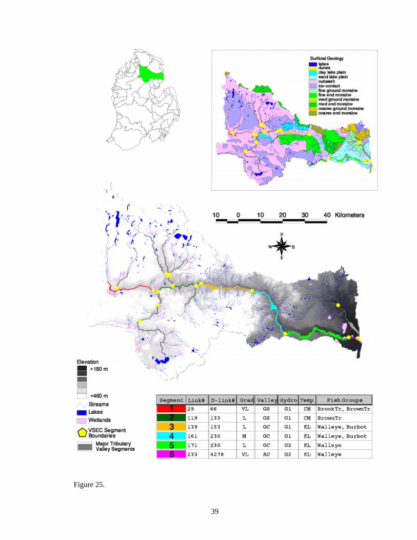
39
Figure 25.

40
Figure 26.

41
Figure 27.
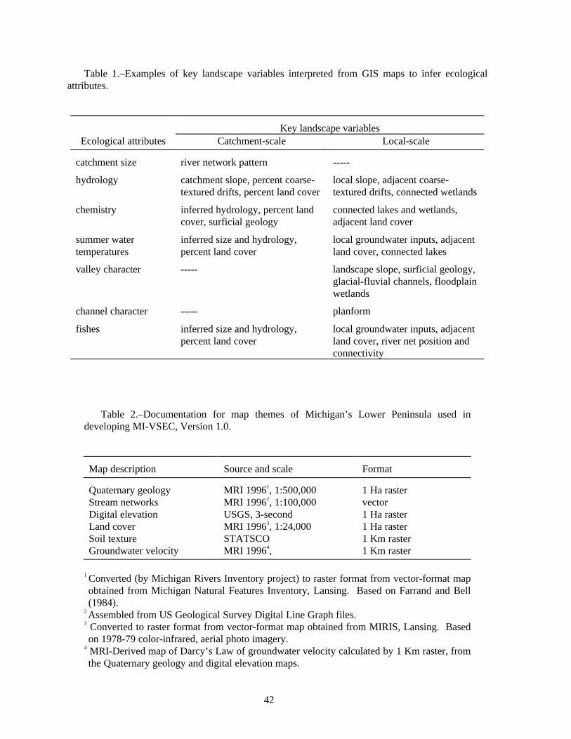
42
Table 1.–Examples of key landscape variables interpreted from GIS maps to infer ecologicalattributes.
Key landscape variablesEcological attributes Catchment-scale Local-scale
catchment size river network pattern -----
hydrology catchment slope, percent coarse-textured drifts, percent land cover
local slope, adjacent coarse-textured drifts, connected wetlands
chemistry inferred hydrology, percent landcover, surficial geology
connected lakes and wetlands,adjacent land cover
summer watertemperatures
inferred size and hydrology,percent land cover
local groundwater inputs, adjacentland cover, connected lakes
valley character ----- landscape slope, surficial geology,glacial-fluvial channels, floodplainwetlands
channel character ----- planform
fishes inferred size and hydrology,percent land cover
local groundwater inputs, adjacentland cover, river net position andconnectivity
Table 2.–Documentation for map themes of Michigan’s Lower Peninsula used indeveloping MI-VSEC, Version 1.0.
Map description Source and scale Format
Quaternary geology MRI 19961, 1:500,000 1 Ha rasterStream networks MRI 19962, 1:100,000 vectorDigital elevation USGS, 3-second 1 Ha rasterLand cover MRI 19963, 1:24,000 1 Ha rasterSoil texture STATSCO 1 Km rasterGroundwater velocity MRI 19964, 1 Km raster
1 Converted (by Michigan Rivers Inventory project) to raster format from vector-format mapobtained from Michigan Natural Features Inventory, Lansing. Based on Farrand and Bell(1984).
2 Assembled from US Geological Survey Digital Line Graph files.3 Converted to raster format from vector-format map obtained from MIRIS, Lansing. Basedon 1978-79 color-infrared, aerial photo imagery.
4 MRI-Derived map of Darcy’s Law of groundwater velocity calculated by 1 Km raster, fromthe Quaternary geology and digital elevation maps.

43
Table 3.–Great Lake basins and major watershed systems described inthe MI-VSEC 1.0 system.
Lake Michigan Basin Lake Huron Basin Lake Erie Basin
St. Joseph Saginaw (lower river) RaisinKalamazoo Cass HuronGrand Shiawassee RougeMuskegon Tittabawassee ClintonWhite Rifle BlackPere Marquette Au SableManistee Thunder Bay
Cheboygan
Table 4.–Statistical fish species associations found in lower Michigan rivers
(Zorn et al. 1997). Group names are in bold.
creek chub redfin shiner stoneroller minnow common shiner bluntnose minnow Johnny darter
flathead catfish white crappie common carp bowfin black crappie tadpole madtom spotted sucker
smallmouth bass black redhorse striped shiner river chub northern hog sucker stonecat greenside darter
mottled sculpin blacknose dace
burbot longnose dace
rosyface shiner yellow perch
white sucker fathead minnow
pumkinseed sunfish black bullhead yellow bullhead green sunfish bluegill
logperch brook silversides mimic shiner shorthead redhorse sand shiner
brown trout chinook salmon rainbow trout
hornyhead chub grass pickerel lake chubsucker
walleye channel catfish spotfin shiner
brook trout slimy sculpin coho salmon
northern pike golden shiner blackside darter central mudminnow pirate perch
golden redhorse greater redhorse silver redhorse
brook stickleback hybrid sunfish northern redbelly dace
rockbass brown bullhead longear sunfish largemouth bass rainbow darter
freshwater drum quillback carpsucker gizzard shad

Tab
le 5
.–C
hara
cter
istic
s of
com
mon
, eco
logi
cal r
iver
val
ley
segm
ent t
ypes
fou
nd in
Low
er M
ichi
gan.
Fis
h as
soci
atio
ns, w
hich
are
dia
gnos
ticof
the
ove
rall
ecol
ogic
al c
hara
cter
of
a se
gmen
t, ar
e em
phas
ized
in
bold
. T
ypes
wer
e ba
sed
on a
n in
itial
sum
mar
y of
MI-
VSE
C h
ydro
logi
c, J
uly
ther
mal
, and
cha
nnel
con
fine
men
t attr
ibut
es.
Sam
pl eH
ydro
logi
cT
herm
alC
hann
elL
ink
Nut
rien
tC
hann
elD
iagn
osti
c
Typ
esi
zere
gim
ere
gim
eco
nfin
emen
tnu
mbe
r ra
nge
code
grad
ient
fish
ass
ocia
tion
s
#1N
=6V
ery
high
gro
undw
ater
Col
d &
Low
dai
ly f
lux
Con
fine
d ch
anne
lL
inks
13-
36O
ligo
trop
hic
Low
gra
dien
tB
rook
tro
ut, B
row
n tr
out
#2N
=6V
ery
high
gro
undw
ater
Col
d &
Low
dai
ly f
lux
Unc
onfi
ned
chan
nelL
inks
10-
14O
ligo
trop
hic
Ver
y lo
w g
radi
ent
Bro
wn
trou
t#3
N=5
Ver
y hi
gh g
roun
dwat
erC
old
& M
oder
ate
dail
y fl
uxC
onfi
ned
chan
nel
Lin
ks 2
3-32
Oli
gotr
ophi
cV
ery
low
/Low
gra
dien
tB
row
n tr
out,
Mot
tled
scu
lpin
#4N
=6V
ery
high
gro
undw
ater
Col
d &
Mod
erat
e da
ily
flux
Unc
onfi
ned
chan
nelL
inks
12-
81O
ligo
trop
hic
Ver
y lo
w/L
ow g
radi
ent
Bro
wn
trou
t
#5N
=7H
igh
grou
ndw
ater
Col
d &
Mod
erat
e da
ily
flux
Con
fine
d ch
anne
lL
inks
6-2
8M
esot
roph
icL
ow/M
oder
ate
grad
ient
Bro
wn
trou
t, M
ottl
ed s
culp
in#6
N=
13H
igh
grou
ndw
ater
Col
d &
Mod
erat
e da
ily
flux
Unc
onfi
ned
chan
nelL
inks
7-2
8M
esot
roph
icV
ery
low
/Low
gra
dien
tB
row
n tr
out,
Mot
tled
scu
lpin
,B
urbo
t, H
orny
head
chu
b#7
N=
11H
igh
grou
ndw
ater
Coo
l & M
oder
ate
dail
y fl
uxU
ncon
fine
d ch
anne
lLin
ks 4
0-11
3M
esot
roph
icV
ery
low
gra
dien
tB
urbo
t, L
ogpe
rch,
Ros
yfac
e sh
iner
,H
orny
head
chu
b
#8N
=6F
air
grou
ndw
ater
Coo
l & M
oder
ate
dail
y fl
uxC
onfi
ned
chan
nel
Lin
ks 9
-18
Eut
roph
icL
ow/M
oder
ate
grad
ient
Mot
tled
scu
lpin
, Hor
nyhe
ad c
hub,
Whi
te s
ucke
r#9
N=
21F
air
grou
ndw
ater
Coo
l & M
oder
ate
dail
y fl
uxU
ncon
fine
d ch
anne
lLin
ks 1
3-77
Mes
otro
phic
Ver
y lo
w/L
ow g
radi
ent
Bur
bot,
Hor
nyhe
ad c
hub,
Log
perc
h, R
osyf
ace,
Roc
kbas
s#1
0N
=6F
air
grou
ndw
ater
War
m &
Mod
erat
e da
ily
flux
Unc
onfi
ned
chan
nelL
inks
36-
80M
esot
roph
icV
ery
low
/Low
gra
dien
tSm
allm
outh
bas
s, R
ockb
ass,
Ros
yfac
e sh
iner
#11
N=
13M
oder
ate
grou
ndw
ater
Coo
l & M
oder
ate
dail
y fl
uxC
onfi
ned
chan
nel
Lin
ks 1
3-91
Eut
roph
icV
ery
low
/Low
gra
dien
tN
orth
ern
pike
, Roc
kbas
s,H
orny
head
chu
b, W
hite
suc
ker
#12
N=
29M
oder
ate
grou
ndw
ater
Coo
l & M
oder
ate
dail
y fl
uxU
ncon
fine
d ch
anne
lLin
ks 1
1-54
Eut
roph
icV
ery
low
/Low
gra
dien
tN
orth
ern
pike
, Roc
kbas
s,H
orny
head
chu
b, W
hite
suc
ker
#13
N=5
Mod
erat
e gr
ound
wat
erW
arm
& M
oder
ate
dail
y fl
uxC
onfi
ned
chan
nel
Lin
ks 3
4-97
Eut
roph
icL
ow g
radi
ent
Smal
lmou
th b
ass,
Roc
kbas
s,R
osyf
ace
shin
er#1
4N
=9M
oder
ate
grou
ndw
ater
War
m &
Mod
erat
e da
ily
flux
Unc
onfi
ned
chan
nelL
inks
14-
68E
utro
phic
Ver
y lo
w/L
ow g
radi
ent
Smal
lmou
th b
ass,
Roc
kbas
s,R
osyf
ace
shin
er, N
orth
ern
pike
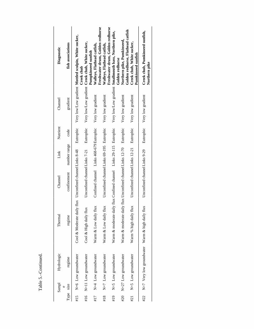
Tab
le 5
.–C
onti
nued
.
Sam
pl eH
ydro
logi
cT
herm
alC
hann
elL
ink
Nut
rien
tC
hann
elD
iagn
osti
c
Typ
esi
zere
gim
ere
gim
eco
nfin
emen
tnu
mbe
r ra
nge
code
grad
ient
fish
ass
ocia
tion
s
#15
N=6
Low
gro
undw
ater
Coo
l & M
oder
ate
dail
y fl
uxU
ncon
fine
d ch
anne
lLin
ks 8
-48
Eut
roph
icV
ery
low
/Low
gra
dien
tM
ottl
ed s
culp
in, W
hite
suc
ker,
Cre
ek c
hub
#16
N=
11L
ow g
roun
dwat
erC
ool &
Hig
h da
ily
flux
Unc
onfi
ned
chan
nelL
inks
7-2
1E
utro
phic
Ver
y lo
w/L
ow g
radi
ent
Cre
ek c
hub,
Whi
te s
ucke
r,P
umpk
inse
ed s
unfi
sh#1
7N
=4L
ow g
roun
dwat
erW
arm
& L
ow d
aily
flu
xC
onfi
ned
chan
nel
Lin
ks 4
68-6
79E
utro
phic
Ver
y lo
w g
radi
ent
Wal
leye
, Fla
thea
d ca
tfis
h,F
resh
wat
er d
rum
, Gol
den
redh
orse
#18
N=7
Low
gro
undw
ater
War
m &
Low
dai
ly f
lux
Unc
onfi
ned
chan
nelL
inks
69-
195
Eut
roph
icV
ery
low
gra
dien
tW
alle
ye, F
lath
ead
catf
ish,
Fre
shw
ater
dru
m, G
olde
n re
dhor
se#1
9N
=5L
ow g
roun
dwat
erW
arm
& m
oder
ate
dail
y fl
uxC
onfi
ned
chan
nel
Lin
ks 2
9-11
5E
utro
phic
Ver
y lo
w/L
ow g
radi
ent
Smal
lmou
th b
ass,
Nor
ther
n pi
ke,
Gol
den
redh
orse
#20
N=
27L
ow g
roun
dwat
erW
arm
& m
oder
ate
dail
y fl
uxU
ncon
fine
d ch
anne
lLin
ks 1
2-70
Eut
roph
icV
ery
low
gra
dien
tN
orth
ern
pike
, Pum
kins
eed,
Gol
den
redh
orse
, Fla
thea
d ca
tfis
h#2
1N
=5L
ow g
roun
dwat
erW
arm
% h
igh
dail
y fl
uxU
ncon
fine
d ch
anne
lLin
ks 1
2-21
Eut
roph
icV
ery
low
gra
dien
tC
reek
chu
b, W
hite
suc
ker,
Pum
kins
eed
sunf
ish
#22
N=7
Ver
y lo
w g
roun
dwat
erW
arm
& h
igh
dail
y fl
uxU
ncon
fine
d ch
anne
lLin
ks 9
-29
Eut
roph
icV
ery
low
gra
dien
tC
reek
chu
b, P
umki
nsee
d su
nfis
h,N
orth
ern
pike

46
Table 6.–Comparisons of terminology for hierarchical terrestrial classification units used byUSFS – National, USEPA, and USFS – Upper Great Lakes States (personal communication, D.A.Albert, Michigan Natural Features Inventory, Lansing). This terminology is still evolving and is notconsistent among geographers. Unit names we have adopted are in parentheses; including a breakingof landtype associations into large- and small-scale categories.
USFS – National USEPA USFS – Upper GL Related aquatic unit
Province
Section Ecoregion Region
Subsection Subregion District
(Sub-subsection) (Landscape-levelecoregion)
Subdistrict sub-watershed
Landtype association –(large)
(Landscape-levelecoregion)
Landtype association –(large)
sub-watershed, valleysegment
Landtype association –(small)
Landtype association –(small)
valley segment

47
References
Albert, D.A. 1994. Regional landscapeecosystems of Michigan, Minnesota, andWisconsin: a working map andclassification. U.S. Forest Service, NorthCentral Forest Experiment Station, GeneralTechnical Report NC-178, St. Paul, MN.
Albert, D.A., Denton, S.R., and B.R. Barnes.1986. Regional landscape ecosystems ofMichigan. University of Michigan, Schoolof Natural Resources, Ann Arbor.
Anonymous. 1981. Michigan streamclassification: 1967 system. Appendix 15 InJ.W. Merna, et al., Editors. Manual offisheries survey methods. MichiganDepartment of Natural Resources, FisheriesManagement Report 9, Lansing.
Anonymous. 1993. National hierarchicalframework of ecological units. U.S.Department of Agriculture, Forest Service,ECOMAP. Washington, D.C.
Bailey, R.G., R.D. Pfister, and J.A. Henderson.1978. Nature of land and resourceclassification—a review. Journal ofForestry 76:650-655.
Baker, ME. 1995. The diversity of landscapeecosystems in river valleys of the Huron-Manistee National Forests, northern lowerMichigan. M.S. Thesis, University ofMichigan, Ann Arbor.
Balon, E.K., and D.J. Stewart. 1983. Fishassemblages in a river with unusual gradient(Luongo, Africa—Zaire system), reflectionson river zonation, and description of anothernew species. Environmental Biology ofFishes 9:225-252.
Barnes, B.V., K.S. Pregitzer, T.A. Spies, andV.H. Spooner. 1982. Ecological forest siteclassification. Journal of Forestry 80:493-498.
Bayley, P.B., and H.W. Li. 1992. Riverinefishes pages 251-281 In P. Calow and G.E.Petts, Editors. The rivers handbook –Volume 1. Blackwell ScientificPublications, Oxford, England.
Bent, P.C. 1971. Influence of surface glacialdeposits on streamflow characteristics. U.S.Geological Survey, Water ResourcesDivision, Open-file Report, Lansing, MI.
Berry, T. 1992. Land use and stream dischargein Michigan’s cold water streams. Masterof Science Thesis, The University ofMichigan, Ann Arbor.
Biggs, B.J.F., M.J. Duncan, I.G. Jowett, J.M.Quinn, C.W. Hickey, R.J. Davies-Colley,and M.E. Close. Ecologicalcharacterization, classification, andmodelling of New Zealand rivers: anintroduction and synthesis. New ZealandJournal of Marine and Freshwater Research24:277-304.
Bowlby, J.N., and J.C. Roff. 1986. Troutbiomass and habitat relationships insouthern Ontario streams. Transactions ofthe American Fisheries Society 115:503-514.
Bryce, S.A., and S.E. Clarke. 1996.Landscape-level ecological regions: linkingstate-level ecoregion frameworks withstream habitat classifications.Environmental Management 20:297-311.
Chamberlin, T.W. 1984. Systematic aquaticbiophysical inventory in British Columbia,Canada. Pages 17-25 In N.B. Armantrout,Editor. Aquisition and utilization of aquatichabitat inventory information. AmericanFisheries Society, Symposium Proceedings,Portland, Or.

48
Corner. R.A., D.A. Albert, C.J. Delain. 1997.Landtype associations of the Leelanau andGrand Traverse peninsulas: SubsectionVII.5. Michigan Natural FeaturesInventory, Technical Report and Map,Lansing.
Cupp, C.E. 1989. Valley segment typeclassification for forested lands ofWashington. Washington Department ofNatural Resources; Timber, Fish andWildlife Ambient Monitoring ProgramReport, Olympia.
Davis, L.S., and J.A. Henderson. 1978. Manyusers and many users: some desirablecharacteristics of a common land and waterclassification system. Pages 13-34 InClassification, inventory and analysis of fishand wildlife habitat. U.S. Fish and WildlifeService, FWS/OBS-78/76, Washington,D.C.
Dewberry, T.C. 1980. A stream classificationsystem for midwestern North America.Unpublished manuscript. (Author’saddress: Pacific Rivers Council, Eugene,Oregon)
Dunne, T., and L.B. Leopold. 1978. Water inenvironmental planning. W.H. Freeman andCo., New York, NY.
Farrand, W.R., and D.F. Eschman. 1974.Glaciation of the southern peninsula ofMichigan: a review. Michigan Academician7:31-56.
Farrand, W.R., and D.L. Bell. 1984.Quaternary geology of southern Michigan.Michigan Department of Natural Resources,Geological Survey Division 1:500,000 Map,Lansing.
Fausch, K.D., J. Lyons, J.R. Karr, and P.L.Angermeier. 1990. Fish communities asindicators of environmental degradation.American Fisheries Society Symposium8:123-144.
Frissell, C.A., W.J. Liss, C.E. Warren, andM.D. Hurley. 1986. A hierarchicalframework for stream habitat classification:viewing streams in a watershed context.Environmental management 10:199-214.
Gowan, D., M.K. Young, K.D. Fausch, and S.C.Riley. 1994. Restricted movement inresident stream salmonids: a paradigm lost?Canadian Journal of Fisheries and AquaticSciences 51:2626-2637.
Hakanson, L. 1996. Predicting important lakehabitat variables from maps using modernmodelling tools. Canadian Journal ofFisheries and Aquatic Sciences 53(Suppl.1):364-382.
Halliwell, D.B. 1989. A classification ofstreams in Massachusetts: “to be used as afisheries management tool”. Ph.D.Dissertation, University of Massachusetts,Amherst.
Harding, E.A. 1984. Landform subdivisions asan interpretive tool for stream and fishhabitat assessment. Pages 41-46 In N.B.Armantrout, Editor. Aquisition andutilization of aquatic habitat inventoryinformation. American Fisheries Society,Symposium Proceedings, Portland, Or.
Hawkes, H.A. 1975. River zonation andclassification. Pages 312-374 In B.A.Whitton, Editor. River Ecology. Universityof California Press, Berkeley.
Hawkins, C.P., J.L. Kershner, P.A. Bisson,M.D. Bryant, L.M. Decker, S.V. Gregory,D.A. McCullough, C.K. Overton, G.H.Reeves, R.J. Steedman, and M.K. Young.1993. A hierarchical approach toclassifying stream habitat features.Fisheries 18:3-11.
Hendrickson, G.E., and C.J. Doonan. 1972.Hydrology and recreation on the cold-waterrivers of Michigan’s southern peninsula.U.S. Geological Survey, Water InformationSeries Report 3, Lansing, MI.

49
Holtschlag, D.J., and H.M. Croskey. 1984.Statistical models for estimating flowcharacteristics of Michigan streams. U.S.Geological Survey, Water-ResourcesInvestigations Report 84-4207, Lansing, MI.
Hudson, P.L., R. W. Griffiths, and T.J.Wheaton. 1992. Review of habitatclassification schemes appropriate tostreams, rivers, and connecting channels inthe Great Lakes drainage basin. Pages 73-107 In W.-D.N. Busch and P.G. Sly,Editors. The Development of an aquatichabitat classification system for lakes. CRCPress, Boca Raton, Florida.
Hughes, R.M., E. Rexstad, and C.E. Bond.1987. The relationship of aquaticecoregions, river basins, and physiographicprovinces to the ichthyogeographic regionsof Oregon. Copeia 1987:423-432.
Kauffman, J.B., R.L. Beschta, and W.S. Platts.1993. Fish habitat improvement projects inthe Fifteenmile Creek and Trout Creekbasins of central Oregon: field review andmanagement recommendations. BonnevillePower Administration, Division of Fish andWildlife Report, DOE/BP-18955-1,Portland, OR.
Kimmins, J.P. 1987. Forest ecology.McMillan Publishing Co., New York, NY.
Kleiman, R. 1995. Modeling water quality inMichigan rivers from landscape variables.M.S. Thesis, University of Michigan, AnnArbor.
Knutilla, R.L. 1970. Statistical summaries ofMichigan streamflow data. U.S. GeologicalSurvey and Michigan Department of NaturalResources, Water Resources Commission,Lansing.
Ladle, M., and D. F. Westlake. 1995. Riverand stream ecosystems of Great Britain.Pages 343-388 In C. E. Cushing, K. W.Cummins and G. W. Minshall, Editors.Ecosystems of the world, 22: River andstream ecosystems. Elsevier, New York.
Larsen, D.P., J.M. Omernik, R.M. Hughes,C.M. Rohm, T.R. Whittier, A.J. Kinney,A.L. Gallant, and D.R. Dudley. 1986.Correspondence between spatial patterns infish assemblages in Ohio streams andaquatic ecoregions. EnvironmentalManagement 10:815-828.
Levin, S.A. 1992. The problem of pattern andscale in ecology. Ecology 73:1943-1967.
Lotspeich, F.B. 1980. Watersheds as the basicecosystem: this conceptual frameworkprovides a basis for a natural classificationsystem. Water Resources Bulletin 16:581-586.
Lotspeich, F.B., and W.S. Platts. 1982. Anintegrated land-aquatic classificationsystem. North American Journal ofFisheries Management 2:138-149.
Lyons, J. 1989. Correspondence between thedistribution of fish assemblages inWisconsin streams and Omernik’secoregions. American Midland Naturalist.122:163-182.
Maxwell, J.R., C.J. Edwards, M.E. Jensen, S.J.Paustian, H. Parrott, and D.M. Hill. 1995.A hierarchical framework of aquaticecological units in North America (NearcticZone). U.S.D.A. Forest Service, North-Central Forest Experiment Station, GeneralTechnical Report NC-176, St. Paul, MN.
Meisner, J.D., J.S. Rosenfeld, and H.A. Regier.1988. The role of groundwater in theimpact of climate warming on streamsalmonines. Fisheries 13:2-8.

50
Minshall, G.W., K.W. Cummins, R.C. Peterson,C.E. Cushing, D.A. Bruns, J.R. Sedell, andR.L. Vannote. 1985. Developments instream ecosystem theory. Canadian Journalof Fisheries and Aquatic Sciences 42:1045-1055.
Naiman, R.J., H.D. DeCamps, J. Pastor, andC.A. Johnston. 1988. The potentialimportance of boundaries to fluvialecosystems. Journal of the North AmericanBenthological Society 7:289-306.
Newsom, M. 1995. Hydrology and the riverenvironment. Oxford University Press, NewYork, NY.
Omernik, J.M. 1987. Ecoregions of theconterminous United States. Annals of theAssociation of American Geographers77:118-125.
Osborne, L.L., and M.J. Wiley. 1992.Influence of tributary spatial position on thestructure of warmwater fish communities.Canadian Journal of Fisheries and AquaticSciences 49:671-681.
Osborne, L.L., S.L. Kohler, P.B. Bayley, D.Day, W. Bertrand, M.J. Wiley, and R.Sauer. 1993. Influence of stream spatiallocation on the Index of Biotic Integrity.Transactions of the American FisheriesSociety 121:635-643.
Poff, N.L., and J.V. Ward. 1989. Implicationsof streamflow variability and predictabilityfor lotic community structure: a regionalanalysis of streamflow patterns. CanadianJournal of Fisheries and Aquatic Sciences46:1805-1818.
Rheaume, S.J. 1991. Hydrologic provinces ofMichigan. U.S. Geological Survey, Water-Resources Investigations Report 91-4120,Lansing, MI.
Richards, R.P. 1990. Measures of flowvariability and a new flow-basedclassification of Great Lakes tributaries.Journal of Great Lakes Research 16:53-70.
Rohm, C.M., J.W. Giese, and C.C. Bennett.1987. Evaluation of an aquatic ecoregionclassification of streams in Arkansas.Journal of Freshwater Ecology 4:127-140.
Rowe, J.S. 1961. The level of integrationconcept and ecology. Ecology 42:420-427.
Rowe, J.S. 1969. Plant community as alandscape feature. Pages 63-81 In K.N.H.Greenidge, Editor. Essays in plantgeography and ecology. The Nova ScotiaMuseum, Halifax.
Rowe, J.S. 1984. Understanding forestlandscapes—what you conceive is what youget. The Leslie L. Schaffer Lectureship inForest Science, University of BritishColumbia, Vancouver.
Rowe, J.S. 1989. What on earth isenvironment? The Trumpeter 6:123-126.
Rowe, J.S. 1991. Forests as landscapeecosystems—implications for theirregionalization and classification. Pages 3-8In Proceedings of a symposium. USDAForest Service, Southeastern ForestExperiment Station, General TechnicalReport SE68, where?
Rosgen, D.L. 1994. A classification of naturalrivers. Catena 22:169-199.
Rowe, J.S., and B.V. Barnes. 1994. Geo-ecosystems and bio-ecosystems. Bulletin ofthe Ecological Society of America 75:40-41.
Schlosser, I.J. 1991. Stream fish ecology: alandscape perspective. BioScience 41:704-712.

51
Schlosser, I.J., and P.L. Angermeier. 1995.Spatial variation in demographic processesof lotic fishes: conceptual models, empiricalevidence, and implications for conservation.American Fisheries Society Symposium17:392-401.
Seelbach, P.W., and M.J. Wiley. 1997.Overview of the Michigan Rivers InventoryProject. Michigan Department of NaturalResources, Fisheries Technical Report 97-3,Ann Arbor.
Spies, T.A., and B.V. Barnes. 1985. Amultifactor ecological classification of thenorthern hardwood and conifer ecosystemsof Sylvania Recreation Area, UpperPeninsula, Michigan. Canadian Journal ofForest Resources 15:949-960.
Statzner, B., and B. Higler. 1985. Questionsand comments on the River ContinuumConcept. Canadian Journal of Fisheries andAquatic Sciences 42:1038-1044.
Strayer, D. 1983. The effects of surfacegeology and stream size on freshwatermussel (Bivalvia, Unionidae) distribution insoutheastern Michigan, U.S.A. FreshwaterBiology 13:235-264.
Threinen, C.W., and R. Poff. 1963. Thegeography of Wisconsin’s trout streams.Wisconsin Academy of Sciences, Arts, andLetters 52:57-75.
Vannote, R.L., G.W. Minshall, K.W. Cummins,J.R. Sedell, and C.E. Cushing. 1980. Theriver continuum concept. Canadian Journalof Fisheries and Aquatic Sciences 37:130-137.
Ward, J.V., and J.A. Stanford. 1983. The serialdiscontinuity concept of lotic ecosystems.Pages 29-42 In T.D. Fontaine and S.M.Bartell (Editors) Dynamics of loticecosystems. Ann Arbor Science Publishers,Inc., Ann Arbor, MI.
Wehrly, K.E., M.J. Wiley, and P.W. Seelbach.1997. Landscape-based models that predictJuly thermal characteristics of lowerMichigan rivers. Michigan Department ofNatural Resources, Fisheries ResearchReport 2037, Ann Arbor.
Wiley, M.J., and P.W. Seelbach. 1997. Anintroduction to rivers. MichiganDepartment of Natural Resources, FisheriesSpecial Report 20, Ann Arbor.
Wiley, M.J., S.L. Kohler, and P.W. Seelbach.1997. Reconciling landscape and localviews of aquatic communities: lessons fromMichigan trout streams. FreshwaterBiology 37:133-148.
Young, R.J., J.R.M. Kelso, and J.G. Weise.1990. Occurrence, relative abundance, andsize of landlocked sea lamprey (Petromyzonmarinus) ammocoetes in relation to streamcharacteristics in the Great Lakes. CanadianJournal of Fisheries and Aquatic Sciences47:1773-1778.
Zorn, T.G., P.W. Seelbach, and M.J. Wiley.1997. Patterns in the fish communities ofLower Michigan streams. MichiganDepartment of Natural Resources, FisheriesResearch Report 2035, Ann Arbor.