a kalman filter calibration method steven c....
TRANSCRIPT

A Kalman Filter Calibration MethodFor Analog Quadrature Position Encoders
by
Steven C. Venema
A thesis submitted in partial fulfillmentof the requirements for the degree of
Master of Sciencein Electrical Engineering
University of Washington
1994
Approved by(Chairperson of Supervisory Committee)
Program Authorizedto Offer Degree
Date

© Copyright 1994
Steven C. Venema

In presenting this thesis in partial fulfillment of the requirements for a Master’s degree atthe University of Washington, I agree that the Library shall make its copies freely availablefor inspection. I further agree that extensive copying of this thesis is allowable only forscholarly purposes, consistent with “fair use” as prescribed in the U.S. Copyright Law. Anyother reproduction for any purposes or by any means shall not be allowed without my writ-ten permission.
Signature
Date


TABLE OF CONTENTS
TABLE OF CONTENTS . . . . . . . . . . . . . . . . . . . . . . . . . . . . . . . . . . . . . . . . . . . . . . . . . . i
LIST OF FIGURES . . . . . . . . . . . . . . . . . . . . . . . . . . . . . . . . . . . . . . . . . . . . . . . . . . . . . iii
LIST OF TABLES . . . . . . . . . . . . . . . . . . . . . . . . . . . . . . . . . . . . . . . . . . . . . . . . . . . . . . . v
Chapter 1: Introduction . . . . . . . . . . . . . . . . . . . . . . . . . . . . . . . . . . . . . . . . . . . . . . . . . . 11.1 Motivation . . . . . . . . . . . . . . . . . . . . . . . . . . . . . . . . . . . . . . . . . . . . . . . . . . . . . . 11.2 Rotary Position Encoders. . . . . . . . . . . . . . . . . . . . . . . . . . . . . . . . . . . . . . . . . . . 1
1.2.1 Functional Overview . . . . . . . . . . . . . . . . . . . . . . . . . . . . . . . . . . . . . . . . 11.2.2 Digital Encoders. . . . . . . . . . . . . . . . . . . . . . . . . . . . . . . . . . . . . . . . . . . . 21.2.3 Analog Encoders . . . . . . . . . . . . . . . . . . . . . . . . . . . . . . . . . . . . . . . . . . . 31.2.4 Nominal Configuration . . . . . . . . . . . . . . . . . . . . . . . . . . . . . . . . . . . . . . 4
1.3 Analog Encoder Calibration . . . . . . . . . . . . . . . . . . . . . . . . . . . . . . . . . . . . . . . . 51.3.1 Non-ideal Encoder Outputs . . . . . . . . . . . . . . . . . . . . . . . . . . . . . . . . . . . 51.3.2 One-to-Many Mapping Problem . . . . . . . . . . . . . . . . . . . . . . . . . . . . . . . 61.3.3 Goals . . . . . . . . . . . . . . . . . . . . . . . . . . . . . . . . . . . . . . . . . . . . . . . . . . . . 6
1.4 Review of Previous Work . . . . . . . . . . . . . . . . . . . . . . . . . . . . . . . . . . . . . . . . . . 81.4.1 Parametric Calibration Method . . . . . . . . . . . . . . . . . . . . . . . . . . . . . . . . 81.4.2 Constant-Velocity Calibration Method . . . . . . . . . . . . . . . . . . . . . . . . . 101.4.3 “Hummingbird” Minipositioner. . . . . . . . . . . . . . . . . . . . . . . . . . . . . . . 121.4.4 Sawyer Sensor . . . . . . . . . . . . . . . . . . . . . . . . . . . . . . . . . . . . . . . . . . . . 12
1.5 Mini Direct-Drive Robot . . . . . . . . . . . . . . . . . . . . . . . . . . . . . . . . . . . . . . . . . . 13
Chapter 2: Problem Analysis. . . . . . . . . . . . . . . . . . . . . . . . . . . . . . . . . . . . . . . . . . . . . 152.1 Noise Model. . . . . . . . . . . . . . . . . . . . . . . . . . . . . . . . . . . . . . . . . . . . . . . . . . . . 152.2 Measurement Noise . . . . . . . . . . . . . . . . . . . . . . . . . . . . . . . . . . . . . . . . . . . . . . 16
2.2.1 Noise Model. . . . . . . . . . . . . . . . . . . . . . . . . . . . . . . . . . . . . . . . . . . . . . 162.2.2 Arctangent of Noisy Measurements. . . . . . . . . . . . . . . . . . . . . . . . . . . . 182.2.3 Variance of Rough Position Estimate . . . . . . . . . . . . . . . . . . . . . . . . . . 202.2.4 Tangent Line Approximation. . . . . . . . . . . . . . . . . . . . . . . . . . . . . . . . . 232.2.5 Approximate Probability Density Function of Intra-Line Position . . . . 242.2.6 Variance of Intra-Line Position . . . . . . . . . . . . . . . . . . . . . . . . . . . . . . . 27
2.3 Calibration Error . . . . . . . . . . . . . . . . . . . . . . . . . . . . . . . . . . . . . . . . . . . . . . . . 29
Chapter 3: Model-Based Calibration Technique. . . . . . . . . . . . . . . . . . . . . . . . . . . . . 303.1 Approach . . . . . . . . . . . . . . . . . . . . . . . . . . . . . . . . . . . . . . . . . . . . . . . . . . . . . . 303.2 Process Model Derivation . . . . . . . . . . . . . . . . . . . . . . . . . . . . . . . . . . . . . . . . . 31
3.2.1 Continuous-Time Model Derivation . . . . . . . . . . . . . . . . . . . . . . . . . . . 313.2.2 Continuous Gauss-Markov Process Model . . . . . . . . . . . . . . . . . . . . . . 323.2.3 Conversion to a Discrete Gauss-Markov Process . . . . . . . . . . . . . . . . . 33
3.3 Kalman Calibration Filter Derivation . . . . . . . . . . . . . . . . . . . . . . . . . . . . . . . . 363.3.1 Measurement Vector . . . . . . . . . . . . . . . . . . . . . . . . . . . . . . . . . . . . . . . 36

ii
3.3.2 Kalman Filter Formulation . . . . . . . . . . . . . . . . . . . . . . . . . . . . . . . . . . 373.3.3 Optimal Smoother Formulation . . . . . . . . . . . . . . . . . . . . . . . . . . . . . . . 38
3.4 Correction Table Generation . . . . . . . . . . . . . . . . . . . . . . . . . . . . . . . . . . . . . . . 39
Chapter 4: Experimental Implementation . . . . . . . . . . . . . . . . . . . . . . . . . . . . . . . . . . 414.1 Experiment Setup. . . . . . . . . . . . . . . . . . . . . . . . . . . . . . . . . . . . . . . . . . . . . . . . 414.2 Data Collection . . . . . . . . . . . . . . . . . . . . . . . . . . . . . . . . . . . . . . . . . . . . . . . . . 42
4.2.1 Trajectory Generation . . . . . . . . . . . . . . . . . . . . . . . . . . . . . . . . . . . . . . 424.2.2 Data Collection Method. . . . . . . . . . . . . . . . . . . . . . . . . . . . . . . . . . . . . 434.2.3 Raw Encoder Data . . . . . . . . . . . . . . . . . . . . . . . . . . . . . . . . . . . . . . . . . 43
4.3 Calibration . . . . . . . . . . . . . . . . . . . . . . . . . . . . . . . . . . . . . . . . . . . . . . . . . . . . . 474.3.1 Kalman/Smoother Parameters . . . . . . . . . . . . . . . . . . . . . . . . . . . . . . . . 474.3.2 Smoother results. . . . . . . . . . . . . . . . . . . . . . . . . . . . . . . . . . . . . . . . . . . 494.3.3 Calibration Table Results. . . . . . . . . . . . . . . . . . . . . . . . . . . . . . . . . . . . 524.3.4 Algorithm Implementation. . . . . . . . . . . . . . . . . . . . . . . . . . . . . . . . . . . 56
Chapter 5: Experimental Results . . . . . . . . . . . . . . . . . . . . . . . . . . . . . . . . . . . . . . . . . 575.1 Off-line Comparison . . . . . . . . . . . . . . . . . . . . . . . . . . . . . . . . . . . . . . . . . . . . . 575.2 Physical Verification . . . . . . . . . . . . . . . . . . . . . . . . . . . . . . . . . . . . . . . . . . . . . 59
5.2.1 Physical Calibration Setup. . . . . . . . . . . . . . . . . . . . . . . . . . . . . . . . . . . 605.2.2 Physical Calibration Data . . . . . . . . . . . . . . . . . . . . . . . . . . . . . . . . . . . 615.2.3 Calibration Table from Physical Calibration . . . . . . . . . . . . . . . . . . . . . 615.2.4 Comparison of Physical Calibration to Kalman Calibration . . . . . . . . . 625.2.5 Relative Precision of Physical and Kalman Calibration . . . . . . . . . . . . 63
5.3 Physical Model Parameter Sensitivity Analysis . . . . . . . . . . . . . . . . . . . . . . . . 65
Chapter 6: Conclusions . . . . . . . . . . . . . . . . . . . . . . . . . . . . . . . . . . . . . . . . . . . . . . . . . 696.1 Summary of work . . . . . . . . . . . . . . . . . . . . . . . . . . . . . . . . . . . . . . . . . . . . . . . 696.2 Advantages of the Kalman Calibration Method . . . . . . . . . . . . . . . . . . . . . . . . 696.3 Future Directions . . . . . . . . . . . . . . . . . . . . . . . . . . . . . . . . . . . . . . . . . . . . . . . . 70
6.3.1 Improved Verification of Calibration Precision . . . . . . . . . . . . . . . . . . 706.3.2 Improved Noise Modeling . . . . . . . . . . . . . . . . . . . . . . . . . . . . . . . . . . . 716.3.3 Embedded System Implementation . . . . . . . . . . . . . . . . . . . . . . . . . . . . 71
REFERENCES . . . . . . . . . . . . . . . . . . . . . . . . . . . . . . . . . . . . . . . . . . . . . . . . . . . . . . . . . 72
APPENDIX A: Van-loan Algorithm Review. . . . . . . . . . . . . . . . . . . . . . . . . . . . . . . . . . 74
APPENDIX B: Matlab Kalman Calibration Implementation. . . . . . . . . . . . . . . . . . . . . . 77

iii
LIST OF FIGURES
Figure 1.1 Encoder Schematic Diagram . . . . . . . . . . . . . . . . . . . . . . . . . . . . . . . . . . . . . 2
Figure 1.2 Nominal Analog Encoder Signal Processing. . . . . . . . . . . . . . . . . . . . . . . . . 4
Figure 1.3 Lissajous plots for typical encoder outputs . . . . . . . . . . . . . . . . . . . . . . . . . . 6
Figure 1.4 Encoder Output “One-to-Many” Mapping Example . . . . . . . . . . . . . . . . . . . 7
Figure 1.5 5-Axis Mini Direct Drive Robot . . . . . . . . . . . . . . . . . . . . . . . . . . . . . . . . . 14
Figure 2.1 Encoder Signal Flow with Error Model. . . . . . . . . . . . . . . . . . . . . . . . . . . . 16
Figure 2.2 Histograms of Encoder Measurement Noise . . . . . . . . . . . . . . . . . . . . . . . . 18
Figure 2.3 Joint Distribution of Encoder Measurement Noise . . . . . . . . . . . . . . . . . . . 19
Figure 2.4 Variance Mapping Problem . . . . . . . . . . . . . . . . . . . . . . . . . . . . . . . . . . . . . 19
Figure 2.5 Tangent-Line Approximation . . . . . . . . . . . . . . . . . . . . . . . . . . . . . . . . . . . 23
Figure 2.6 Coordinate System Rotation of Joint Gaussian PDF . . . . . . . . . . . . . . . . . . 24
Figure 2.7 3-Sigma Contour of Rough Position vs. Rough Position . . . . . . . . . . . . . . 28
Figure 3.1 Kalman Calibration Algorithm Schematic. . . . . . . . . . . . . . . . . . . . . . . . . . 30
Figure 4.1 Experiment Configuration . . . . . . . . . . . . . . . . . . . . . . . . . . . . . . . . . . . . . . 41
Figure 4.2 Lissajous Plot of Experiment Data . . . . . . . . . . . . . . . . . . . . . . . . . . . . . . . 44
Figure 4.3 Spiraled Lissajous Plot of Raw Encoder Data (1-second) . . . . . . . . . . . . . . 45
Figure 4.4 Rough State Estimates and Commanded Motor Current. . . . . . . . . . . . . . . 46
Figure 4.5 State Variance and Kalman Gain plot . . . . . . . . . . . . . . . . . . . . . . . . . . . . . 50
Figure 4.6 Smoothed Velocity Estimate . . . . . . . . . . . . . . . . . . . . . . . . . . . . . . . . . . . . 51
Figure 4.7 Acceleration Estimate . . . . . . . . . . . . . . . . . . . . . . . . . . . . . . . . . . . . . . . . . 51
Figure 4.8 Measurement Noise Estimate . . . . . . . . . . . . . . . . . . . . . . . . . . . . . . . . . . . 52
Figure 4.9 Raw Calibration Table . . . . . . . . . . . . . . . . . . . . . . . . . . . . . . . . . . . . . . . . . 53
Figure 4.10 Velocity-Filtered Calibration Table. . . . . . . . . . . . . . . . . . . . . . . . . . . . . . . 54
Figure 4.11 Smoothed Resampled Correction Function, . . . . . . . . . . . . . . . . . . . . . . . . 55
Figure 5.1 Position Error Residuals Before and After Correction . . . . . . . . . . . . . . . . 58
Figure 5.2 Velocity Estimate Comparison . . . . . . . . . . . . . . . . . . . . . . . . . . . . . . . . . . 59

iv
Figure 5.3 Physical Calibration Setup. . . . . . . . . . . . . . . . . . . . . . . . . . . . . . . . . . . . . . 60
Figure 5.4 Physical Calibration Data: (a,b) Values vs. Displacement . . . . . . . . . . . . . 62
Figure 5.5 Calibration Table from Physical Calibration . . . . . . . . . . . . . . . . . . . . . . . . 63
Figure 5.6 Comparison of Kalman Calibration with Physical Calibration . . . . . . . . . . 64
Figure 5.7 Calibration Comparison after Encoder Reassembly . . . . . . . . . . . . . . . . . . 65
Figure 5.8 Velocity Estimate from Physical Calibration Table . . . . . . . . . . . . . . . . . . 66
Figure 5.9 Calibration Table Sensitivity to Changes in Inertia (J) . . . . . . . . . . . . . . . . 67
Figure 5.10 Calibration Table Sensitivity to Changes in Damping (BF) . . . . . . . . . . . . 67
Figure 5.11 Calibration Table Sensitivity to Changes in Torque Constant (KT) . . . . . . 68

v
LIST OF TABLES
Table 1: Examples of Inter-Line Position Computation. . . . . . . . . . . . . . . . . . . . . . . . . . 45
Table 2: Physical Model Parameters. . . . . . . . . . . . . . . . . . . . . . . . . . . . . . . . . . . . . . . . . 47

vi
ACKNOWLEDGEMENTS
I want to express my appreciation and gratitude to my advisor and committee chair,
Professor Blake Hannaford, for his patient and thorough technical and editing advice dur-
ing the preparation of this thesis. Thanks also to Professors Deirdre Meldrum and Juris
Vagners for taking the time to serve on my committee and for their many helpful sugges-
tions. I also want to thank Frederik Boe, Dal-Yeon Hwang, and Darwei Kung for their
willingness to act as “sounding boards” for many of the ideas put forth in this thesis. Final-
ly, and most importantly, I want to thank my wife Meg and daughters Katie and Liz for their
love, support, and tolerance during the several busy months that thesis was being written.
The development of this thesis was partially supported by the National Science Foun-
dation through a PYI research grant awarded to Professor Blake Hannaford.

CHAPTER 1: INTRODUCTION
1.1 Motivation
The need for precision position sensors is driven by a variety of industries that require
precision motion. Rotary position sensors are especially common since the majority of pre-
cision motion devices are driven by rotary motors. Typically, a rotary electromagnetic
motor drives either a rotary or linear motion stage using some sort of gearing arrangement.
If the gearing ratio between the motor and the motion stage is high, then a relatively low
resolution rotary position sensor at the motor will result in high resolution motion measure-
ments at the motion stage. However, backlash in the gearing system will limit precision.
New technological demands in diverse fields such as multi-chip semiconductor mod-
ules and biomedical genetics research have motivated the development of small, direct-
drive motion systems with very high positioning resolution. The lack of gearing in these
system implies that higher resolution position sensors are needed to achieve the higher po-
sitioning precision.
Sensors with analog quadrature outputs are of particular interest for high-precision po-
sitioning because their analog nature allows a degree of interpolation between the
quadrature phases. However, this type of sensor suffers from nonlinear effects which are
difficult to calibrate out. The objective of this thesis is the development of a new technique
for the in-situ calibration of analog quadrature position sensors. The analog rotary incre-
mental optical encoder is used as the example for this analysis; however the calibration
technique is applicable to many other analog quadrature sensors.
1.2 Rotary Position Encoders
1.2.1 Functional Overview
The rotary incremental optical encoder consists of three basic components: a slotted
disk, a light source, and a dual light-detector configured as shown in Figure 1.1. A light
source shines on a disk which is covered with an evenly-spaced radial pattern of transmis-
sive and reflective/absorptive elements called “encoder lines.” Lower resolution encoders
use a metal disk with radially-cut slots to vary optical transmissivity of the disk. Higher res-

2
olution encoders typically use a radial pattern of chromium lines evaporated onto clear
glass. A dual light detector array on the opposite side of the disk detects varying intensities
of light as the disk rotates due to the pattern on the disk. The two detectors are placed 0.25
of a line apart so that the peak output signal of one detector occurs 0.25 of a line before/
after the other (i.e., the outputs of the two detectors are in quadrature phase). This type of
optical encoder was made feasible by the development of solid state light sources and photo
detectors.
A typical encoder installation consists of mounting the light source and detector array
on a fixed frame such as a motor body and mounting the encoder disk on the motor’s rotor
shaft. As the rotor turns, the encoder disk turns as well, alternately obstructing and trans-
mitting light between the light source and the detectors. The detectors output two
quadrature signals, called and , which are correlated with the intensity of the light strik-
ing each of the two detectors. These signals can then be used together to determine
the rotary position of the motor shaft as described below. Linear versions of this type of
sensor are also possible, using a lines on a linear bar instead of a rotating disk.
1.2.2 Digital Encoders
Most incremental encoders in use today are digital encoders. In this type of encoder, the
two detector outputs are converted into digital quadrature signals using thresholding cir-
LightSource
QuadratureLight Detector
RotatingEncoder Disk
AnalogOutputs (a,b)
Figure 1.1:Encoder Schematic Diagram
a b
a b,( )

3
cuits. These signals are then fed into a quadrature decoder logic circuit which monitors the
two signals for changes in logic level. Due to the quadrature phase between the two signals,
position changes of 0.25 of a line may be converted to pulses on separate clockwise (CW)
and counterclockwise (CCW) signals. These position change signals are fed into “up” and
“down” inputs of a digital counter which maintains an absolute position count in units of
0.25 of a line relative to some predefined 0 rotational position.
Logic chips such as Hewlett-Packard’s HCTL2016 [1] are available which contain both
the quadrature decoder logic and the digital counter as well as a byte-wide output port suit-
able for direct interface to a microprocessor.
1.2.3 Analog Encoders
The primary difference between an analog incremental rotary encoder and its digital
counterpart is that the detector outputs are not internally thresholded into digital quadrature
signals. Instead, the analog quadrature signals are typically passed through operational am-
plifiers within the encoder which perform signal conditioning (offset and gain adjustments)
and drive the output lines.
Ideally, the output signals from two detectors are sinusoidal waveforms in quadrature
phase which go through one cycle per encoder-disk line as the disk rotates. Assuming that
the signal is symmetric about 0-volts, the zero-crossings of the two signals can be used like
the transitions in the digital quadrature signal to determine rotary position to 0.25-line res-
olution. However, the analog values of the two signals can be used to further interpolate the
intra-line position to much higher resolutions.
This ability to interpolate between lines is the primary advantage of analog encoders: it
multiplies the angular resolution afforded by the lines on the encoder disk by whatever
amount of resolution that can be interpolated between a pair of lines. For example, if an
encoder has lines then the digital resolution would be
(1-1)
However, if the analog signals are used to interpolate the intra-line position to, for example,
NL 1000=
RD
360Degrees
Revolution--------------------------
1000Lines
Revolution--------------------------
4Transitions
Line---------------------------
×----------------------------------------------------------------------------------------- 0.09
DegreesTransition------------------------
= =

4
one part in 100, then the angular resolution can be improved to
, (1-2)
a factor of 25 improvement in angular resolution.
1.2.4 Nominal Configuration
The outputs of an analog encoder are periodic in angular distance with a fre-
quency of , the number of lines on the encoder disk. In order to obtain a position
measurement, some standard hardware is needed to process these signals. Figure 1.2 shows
a typical configuration. Each of the encoder outputs is passed through a threshold-
ing circuit which emulates the thresholding circuits found in digital encoders. The
thresholded versions of these signals are then treated just like the signals from a digital en-
coder as discussed in Section 1.2.2 above, connecting to a quadrature decoder which, in
turn, drives a digital counter. The counter value is used as an estimate of the encoder posi-
tion, . The least significant bit of the counter represents 0.25 of an encoder line so the
digital position estimate, (in units of encoder lines) is the digital value of the counter,
divided by four:
RA
360Degrees
Revolution--------------------------
1000Lines
Revolution--------------------------
100Transitions
Line---------------------------
×----------------------------------------------------------------------------------------------- 0.0036
DegreesTransition------------------------
= =
a b,( )
NL
EncoderOutputs (a,b)
ThresholdingCircuit
DualA/D
DigitalQuadrature
Decoder
(HCTL 2016)/16
Converter
/12
/12
PositionInterpolation
Data
DigitalPositionCounter
Figure 1.2:Nominal Analog Encoder Signal Processing
a
bbd
ad
pc
a b,( )
p
pd
pc

5
(1-3)
The signals from the encoder are also passed directly to a digitizing circuit
which converts their analog voltages to digital equivalents. The digitized values are then
used to generate a more accurate intra-line interpolation of the encoder position. Special
care must be taken so that the signals are sampled simultaneously to avoid changes
in apparent position due to a time lag between samples.
1.3 Analog Encoder Calibration
1.3.1 Non-ideal Encoder Outputs
Most manufacturers of analog encoders claim that their devices output sinusoidal
waveforms. Ideally, the two sinusoids would have exactly the same frequency ( ) and
amplitude ( ) and differ in phase by exactly 90°. These ideal signals could then be mod-
eled by,
(1-4)
where is the distance between an adjacent pair of encoder lines, normalized to the real
interval [-0.5,+0.5). Assuming that the output signals accurately follow this model, the in-
tra-line distance can be determined using the two-argument arctangent function to avoid
quadrant ambiguity problems:
. (1-5)
In reality, the output signals of the analog encoders, and rarely match the
ideal quadrature sinusoid model of (1-4). The output waveform is very sensitive to the rel-
ative distance and alignment between the light-source and the encoder-disk and between
the encoder-disk and the quadrature photodetectors. Most high-resolution analog encoders
are sold as pre-assembled units with high-precision bearings to minimize these alignment
distortions. “Kit” encoders are assembled by the customer and are very difficult to align
correctly. Even in the pre-assembled units, the encoder signals rarely match the ideal sinu-
soidal model given in (1-4).
pd
pc
4-----=
a b,( )
a b,( )
2π
α
a τ( ) α 2πτ( )sin=
b τ( ) α 2πτ( )cos=
τ
τ 2 a b,( )atan2π
------------------------------=
a τ( ) b τ( )

6
The outputs of 3 different encoders are shown as Lissajous plots ( vs. ) in Figure
1.3. The left-most figure is from a 1024-line factory-assembled encoder with high-preci-
sion bearings. The remaining two figures are 1000-line hollow-shaft “kit” encoders
mounted with the light emitter and detectors bolted to the motor body and the encoder disk
mounted on the motor shaft. The dotted-circular shape is the output from an ideal encoder
characterized by (1-4). These plots demonstrate that the kit encoders output waveforms are
further from the ideal circle than the factory-assembled encoder, but all three encoders suf-
fer from non-ideal characteristics.
1.3.2 One-to-Many Mapping Problem
At first glance it seems that one could use the Lissajous plot directly to determine the
intra-line position. However, without an accurate model of the encoder signals, and
, it is impossible to accurately map these signals to the intra-line position, . This is
illustrated graphically in Figure 1.4 which shows that it is possible to invent two functions
and which map to the same Lissajous plot. In fact, any num-
ber of functions can map to the same Lissajous plot. This implies the converse
as well: it is impossible to use the Lissajous plot alone to determine intra-line position,
for a given encoder time sample, .
1.3.3 Goals
Experience has shown that analog encoder output signals roughly approximate the ideal
a b
Figure 1.3:Lissajous plots for typical encoder outputs
a τ( )
b τ( ) τ
a1 τ( ) b1 τ( ),[ ] a2 τ( ) b2 τ( ),[ ]
a τ( ) b τ( ),[ ]
τ
a t( ) b t( ),[ ]

7
model given in (1-4). If this ideal model is used to generate a rough intra-line position es-
timate, , using (1-5), the true intra-line position may be modeled as
(1-6)
where is a calibration term which corrects for the estimate error in due to the use
of the ideal model.
The goal of this thesis is the development of a robust technique to accurately determine
the calibration function for an analog encoder which
τ
b τ( )b τ( )
a τ( )
τ
a τ( )
Figure 1.4:Encoder Output “One-to-Many” Mapping Example
LEGEND
samples
samples
Combined samples
a1 b1,[ ]
a2 b2,[ ]
τa
τ τa ε τa( )+=
ε τa( ) τa
ε τa( )
8
1. does not require expensive and time-consuming external calibration hardware such
as micrometers or laser interferometers,
2. applies to any analog encoder (even the ones with highly non-circular Lissajous
plots),
3. may be used on encoders in their final installed configuration (since the encoder
output functions may change with each installation), and
4. uses the same signal measurement hardware and sampling rates as the final control
system so that calibration can be performed in the final installed system at any
time.
1.4 Review of Previous Work
1.4.1 Parametric Calibration Method
A parametric calibration algorithm for analog optical encoders was developed by P.
Marbot in [2] for use in a 3 degree-of-freedom direct-drive minirobot. The algorithm as-
sumes that the encoder outputs are sinusoidal as in (1-4), but relaxes the 90° phase and the
equal-amplitude constraints. The outputs are modeled by the functions,
(1-7)
where the amplitudes, , and the quadrature phase error, , are constant but unique
to each encoder and mounting configuration. The Lissajous plot of the outputs of
this model forms an ellipse where the parameters control the length of the major
and minor axes and the parameter controls the amount of rotation. Using this modified
model, Marbot first rewrites the second equation in (1-7) as
(1-8)
by trigonometric identity and then solves for :
. (1-9)
Equation (1-9) can be rearranged algebraically to
a τ( ) α 2πτ( )cos=
b τ( ) β 2πτ Φ–( )sin=
α andβ Φ
a b,( )
α β,( )
Φ
b τ( ) β 2πτ( )sin Φ( )cos β Φ( )sin 2πτ( )cos–=
τ
b τ( )a τ( )--------- β 2πτ( )sin Φ( )cos β Φ( )sin 2πτ( )cos–
α 2πτ( )cos-------------------------------------------------------------------------------------------------------=
βα--- 2πτ( )tan Φ( )cos
βα--- Φ( )sin–=

9
(1-10)
so that
. (1-11)
The new encoder model in (1-11) was applied to factory-assembled encoders with out-
put waveforms similar to that shown in the left-most Lissajous plot in Figure 1.3. Marbot
named this model the “Potato Algorithm” since it partially corrects for the potato-like shape
of the Lissajous plot of his encoder outputs. Note that it is the unequal amplitudes
of the two signals which gives the plot its elliptical shape and the phase error that
causes the rotated orientation of the ellipse. If the amplitudes are exactly equal and there is
no phase error, then the plot would form a perfect circle. In this case, the ideal model in (1-
5) would be applicable.
The Potato algorithm was implemented by lookup table on an 8-bit microcontroller
(Motorola 68HC11) and increased the intra-line resolution by a factor of 16 over the stan-
dard 0.25-line resolution of a digital encoder while running at a rate of 1000 Hz. An off-
line calibration procedure was used to find the model parameters, . This calibra-
tion required multiple samples from a moving encoder to be uploaded from the
microcontroller to a personal computer via a serial port where the amplitude and phase es-
timates were made by examining the maximum values and phase difference between the
two signals for a single cycle.
Marbot points out the following important features of this “potato algorithm”:
1. The parameters are constant for a given encoder and mounting configu-
ration. Once these parameters are identified, much of the computational complex-
ity of (1-11) can be reduced by precomputing the constant terms such as and
. This was especially important in view of the relatively low computational
performance of the selected microcontroller (0.5MIPS, 16-bit integer arithmetic)
and the high servo rate (1000 Hz.). Precomputed lookup tables for some of the
sub-expressions of (1-11) were also used to increase computational performance.
2. The model assumes that the encoder signals are symmetric about the origin (i.e.,
2πτ( )tan αb τ( )βa τ( ) Φ( )cos---------------------------------- Φ( )tan+=
τ 2 αb τ( ) βa τ( ) Φsin+ βa τ( ) Φcos,( )atan2π
-------------------------------------------------------------------------------------------------=
α β≠( )
Φ 0≠( )
α β Φ, ,[ ]
α β Φ, ,[ ]
Φsin
Φcos

10
the potato shape in the Lissajous plot is centered at the origin). If either of the sig-
nals have some small amount of offset, this should be subtracted out before being
passed to the model.
3. The parameters are expressed in (1-10) as a ratio. Therefore, this algo-
rithm is implicitly insensitive to common-mode changes in the peak-to-peak
amplitude of the encoder signals.
Using the Potato algorithm on factory assembled encoders, Marbot was able to increase
resolution by a factor of 16 (4-bits) over the 0.25-line digital resolution. However, a better
method of calibration is needed if higher precision interpolation is desired or if the output
of an encoder deviates significantly from the ellipsoidal shape assumed by (1-11).
1.4.2 Constant-Velocity Calibration Method
Hagiwara, et.al., developed a lookup-table based calibration (“code compensation”)
technique in [3]. The paper discusses the design of a hardware encoder interface which per-
forms the following functions:
1. Reads the analog encoder signals at a 100-kHz rate, converting them to
digital values using A/D converters.
2. Uses the digital values as an index into a ROM-based lookup table which
contains the arctangent function.
3. Uses the output of the arctangent table as an index into a ROM-based lookup table
of correction factors.
4. Combines the outputs of the two ROM lookup tables into an estimated position
output using a collection of adders, latches, and counters.
This digital interface hardware computes an interpolated intra-line position by first assum-
ing an ideal encoder model (i.e., equation (1-5) using the first ROM), and then subtracting
off the error between the ideal model and true position using the second ROM lookup table.
Additional adders, latches, and counters are used to keep track of the incremental rotary po-
sition in a manner similar to that of the HCTL 2016 chip mentioned in Section 1.2.2.
The index (actually a digital address) for the first ROM, is formed by combining the
two digitized encoder values using the relation,
α β,[ ]
a b,( )
a b,( )
ad bd,( )

11
(1-12)
where is the number of significant bits from the A/D converter. This maps all possible
A/D value-pairs to unique addresses, implying that the ROM must have a depth
of words. The values at each address correspond to a conveniently scaled relation,
, and the accuracy is limited to the ROM width. Hagiwara, et.al. used 6-bit
A/D converters and an 8-bit ROM, requiring a -bit ROM for the first lookup table.
The 8-bit ROM width limited the intra-line interpolation precision to or 256 unique
locations.
The contents of the second, “correction-factor” ROM were generated by high-speed
sampling (100 kHz) of the encoder outputs while the encoder was spinning at about 9 lines
per second to yield about 220 samples per line. By assuming that the rotational velocity was
constant over the sampling ensemble, a “true” position was computed by integrating the av-
erage velocity (i.e., ). The correction
factor for a given ideal-model position (e.g., ) was then the difference be-
tween the ideal-model position and the integrated position for a given sample. The error for
each ideal-model position (256 possible positions due to the 8-bit width of the first ROM)
was computed over multiple experiments and averaged to generate a final lookup table of
correction factors.
Using this method on a 3600-line encoder, an 8-bit (256 element) correction table was
generated. Experimental confirmation of the accuracy of this correction table indicated that
there were residual errors of 3 counts (about 3 bits). This implies that only the upper 5-
bits of the 8-bit correction table were significant, yielding an intra-line resolution of
, a factor of 8 increase in intra-line resolution over the 0.25-line resolution of a
digital encoder. Regarding the 3-count error in the calibration table, Hagiwara concluded
that,
As every phase code is compensated, the deviation is expected to be less thancount. But in experiments, so far as this time, we have not been successful in min-imizing the error to this level. This may be caused by noise and the fluctuation ofthe rotating speed which we assumed to be constant.
AROM1 2m
ad×
bd+=
m
ad bd,( )
22m
2 ad bd,( )atan
4096 8×
1 28⁄
average-velocity sample-interval× sample-number×
2 ad bd,( )atan
25
32=
1±

12
1.4.3 “Hummingbird” Minipositioner
Karidis, et.al. developed a specialized quadrature rotary position encoder as part of their
“Hummingbird” Minipositioner [4], a small ( mm work volume), high-perfor-
mance (>50-G accelerations) manipulator for high-precision positioning (1-µm)
applications. The encoder uses the same principles as a typical rotary optical encoder such
as the one shown in Figure 1.1. However the optical path is slightly different with the light
passing from the LED through a grid-plate (instead of a rotary disk), to a corner reflector
which sends the light back through a second grid plate, to a pattern of 4 photodetectors
which generate two differential quadrature signals as a function of position.
The encoder line resolution is 10 lines per degree, yielding a digital resolution of 0.025
degrees. Karidis, et.al. state that they are able to utilize intra-line interpolation to increase
resolution to 0.00089 of a degree, a factor of 29 improvement. However no mention is
made of the calibration method used for their encoder.
1.4.4 Sawyer Sensor
The Sawyer motor [5] is a planar motion analog to the rotary stepper motor. A polished,
flat steel surface, called a “platen” acts as the stator. The surface is inscribed with a fine
rectangular grid which acts as the stator’s “teeth”. The motor contains an arrangement of
electromagnets and linearly arranged, quadrature-phased groups of magnetic “teeth” that
allow it to move along and slightly above the plane of the steel platen by interacting with
an air bearing. The magnitude and phasing of the current profiles in the electromagnets con-
trol motion along the two cartesian degrees of freedom as well as a small amount of
orientation around the axis perpendicular to the platen. As with traditional rotary stepper
motors, the Sawyer motor supports open-loop position-control as well as micro-stepping
control modes. However, the finest stepping precisions are prone to errors (e.g., missed
steps) so some sort of position sensing is desirable.
J. Ish-Shalom [6] developed a Sawyer sensor for use with the Sawyer motor. The sensor
uses the same type of structure as the Sawyer motor: groups of magnetic teeth in quadrature
phase (relative to the tooth pitch) act as a variable magnetic reluctance sensor, with a high-
frequency magnetic field from a driver coil acting as the magnetic signal source. The sensor
13 13 1××

13
outputs two signals in quadrature phase which are periodic in distance relative to the pitch
of the platen teeth.
The Lissajous plot of the Sawyer sensor signals, as shown in [6], appears very similar
to the middle plot of Figure 1.3. Ish-Shalom used a laser interferometer system to calibrate
non-ideal properties of the output signals relative to an ideal sinusoidal function similar to
(1-4). The error correction values, as defined by the difference between the interferometer-
measured position and the ideal sinusoidal model position, were fitted to a 3rd order poly-
nomial. This polynomial was then used to generate corrections from the ideal model for
future position measurements.
Ish-Shalom tested the sensor on an experimental system with 1-mm pitch lines on the
platen, implying a standard digital resolution of 250-µm. He reports maximum errors of
less than -µm using the 3rd-order polynomial model for intra-line interpolation, a factor
of 250 improvement over the digital position estimate.
1.5 Mini Direct-Drive Robot
Marbot [2] developed a miniature 3 degree-of-freedom (DOF) biomedical research ro-
bot for high-precision manipulation of small fluid samples using thin glass pipettes. Direct-
drive motors and precision sensors were used on its three joints to maximize positioning
control and resolution over its 17-cm3 work volume. The first joint was a prismatic (linear
motion) joint and used an LVDT positioning sensor. The other two joints were revolute and
used analog quadrature encoders for position sensing. These factory assembled encoders
(Model CP-320-1024 from Computer Optical Products, Inc. (COPI) of Chatsworth Califor-
nia) produced Lissajous plots similar to the one shown in the left-most plot of Figure 1.3.
The “Potato” algorithm described in Section 1.4.1 was used to calibrate these analog
encoders.
This minirobot has subsequently been upgraded to incorporate a 2-axis wrist, for a total
of 5 joints to be used in more demanding biomedical research tasks as well as a general re-
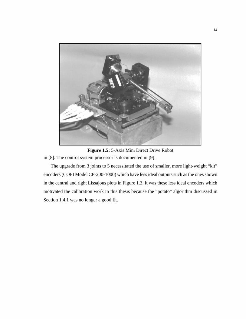
search tool for scaled teleoperation. Figure 1.5 shows the current physical implementation
of the robot. A general overview of the design and implementation of the robot and its con-
trol system may be found in [7]. The mechanism design and implementation is documented
1±
14
in [8]. The control system processor is documented in [9].
The upgrade from 3 joints to 5 necessitated the use of smaller, more light-weight “kit”
encoders (COPI Model CP-200-1000) which have less ideal outputs such as the ones shown
in the central and right Lissajous plots in Figure 1.3. It was these less ideal encoders which
motivated the calibration work in this thesis because the “potato” algorithm discussed in
Section 1.4.1 was no longer a good fit.
Figure 1.5:5-Axis Mini Direct Drive Robot

CHAPTER 2: PROBLEM ANALYSIS
In Section 1.3, Lissajous plots for several analog encoders were shown which each have
a different non-circular shape. The variations in output waveforms between different en-
coders motivates the development of a general calibration method to determine intra-line
position. One way to view this calibration problem is to model the intra-line position as giv-
en in (1-6):
, (2-1)
Here the true intra-line position, , is modeled as the sum of a rough intra-line position, ,
as determined by the ideal model in (1-4) and , a calibration term which compensates
for the non-ideal properties of the encoder. The challenge is to determine this calibration
function, , for . A new approach to determining this function in the
form of a lookup table is presented in the next chapter. However, before this approach is
presented, it is important to understand the final limitations on any calibration approach.
2.1 Noise Model
The use of intra-line interpolation of the ideal analog encoder allows theoretically infi-
nite angular position resolution. However, the limitations of manufacturing tolerance,
measurement noise, quantization error, and calibration errors in real encoders provide
physical limitations to position resolution. The purpose of this chapter is to analyze the
sources of error in the process of intra-line position estimation for non-ideal encoders.
Figure (2-1) shows that the accuracy of the actual intra-line position, , is dependent
on the accuracy of both the measured rough position estimate, , and the calibration term,
. Since is a computed function of the encoder signal measurements which
are themselves subject to measurement noise, is an inherently stochastic signal. The cal-
ibration function, , is also stochastic because noise in will cause the incorrect
calibration term, , to be extracted from the function. Also, may be imperfectly
known due to errors in the calibration process or due to variations in the line width and in-
tra-line distance on the encoder disk. The noise on the encoder signals is
measurement noise, and the error in the correction factor, , iscalibration error. Quan-
tization noise from the A/D conversion is not specifically modeled; however, it can be
τ τa ε τa( )+=
τ τa
ε τa( )
ε τa( ) 0.5 τa 0.5<≤–
τ
τa
ε τa( ) τa a b,( )
τa
ε τa( ) τa
ε ε τa( )
a b,( )
ε τa( )

16
lumped together with the measurement noise for the purposes of the following analysis.
Using the above definitions, the effects of these errors on the final intra-line position
estimate, , can be analyzed. Figure 2.1 shows the signal flow for the intra-line estimator
in the nominal configuration (see Section 1.2.4). The measurement noise is shown as addi-
tive noise in the encoder analog outputs which is then quantized by the A/D converters and
used to compute using the ideal encoder model relation in (1-5). The calibration noise
is shown as additive noise to the corrected intra-line position estimate, .
2.2 Measurement Noise
2.2.1 Noise Model
The analog encoder signals are generated by optical receivers within the encoder. These
signals must pass through a variety of amplifiers and cables before finally reaching A/D
converters. Noise may added at any stage of this signal path due to internal amplifier noise
and electromagnetic interference (EMI) in cable transmission lines. The noisy signals are
then sampled at periodic intervals by the A/D converters.
It is convenient to model the discrete measurements, , as the sum of determin-
istic signals, , and some stationary noise sources with zero-mean gaussian
distributions using the relations,
(2-2)
τ
EncoderOutputs (a,b)
DualA/D
Converters
Figure 2.1:Encoder Signal Flow with Error Model
+
+
MeasurementNoise
+
CalibrationError
Intra-LinePositionEstimate
2 bd ad,( )atan
2π-------------------------------
τaτ
CalibrationTerm
ε τa( )
ad
bd
a
b
Table
MeasurementNoise
bn
anζ
τa
τ
ad bd,( )
a t( ) b t( ),( )
ad t( ) a t( ) an t( )+=
bd t( ) b t( ) bn t( )+=
17
where
(2-3)
and are the variances of the two noise sources. Since and are each a sum of
a deterministic variable and a gaussian random variable, and since a linear function of a
gaussian random variable is also gaussian, and are also gaussian random variables.
Thus (2-2) can be rewritten as
. (2-4)
In order to justify this model, some experimental data is needed. By holding the encoder
position constant, the statistical properties of the measurement noise on an experimental en-
coder may be studied. Approximately 3000 samples of the signals for a stationary
analog encoder were taken at 1-millisecond intervals. Figure 2.2 shows the histograms of
each of the encoder signals with one bin per A/D unit. The plots show roughly gaussian dis-
tributions with two different mean values which are the stationary and
deterministic positions in (2-3). Numeric computations of the variance in the two signals
yield
(2-5)
using and as defined in (2-3). The variances of the two signals are quite different; this
was found to be the case for several different encoders at various intra-line positions using
the same experimental configuration. The source of this difference was traced to the actual
encoder outputs (i.e., it is not due to noise in the experimental electronics) but the cause of
this difference is unknown.
Another important aspect of the measurement noise is the degree of correlation between
the two noise sources as modeled in (2-2). Figure 2.3 shows the joint distribution of the ex-
perimental dataset as both a mesh plot and a contour plot. The fact that the major and minor
axes of the constant probability ellipses in the contour plot align with the measurement axes
an N 0 A,( )=∆
bn N 0 B,( )=∆
A B,( ) ad bd
ad bd
ad t( ) N a t( ) A,( )=
bd t( ) N b t( ) B,( )=
ad bd,( )
a t( ) b t( )
A 1.68=
B 3.04=
A B

18
indicates that the two random noise sources are highly uncorrelated. The computed corre-
lation coefficient, , confirms this observation. The low correlation implies that
the random variables used to model the two gaussian noise sources are independent. When
are combined together to compute , the independence of these random vari-
ables allows for an improved estimate of .
2.2.2 Arctangent of Noisy Measurements
The rough intra-line position, , as defined in (2-1), is computed using the ideal
model:
, (2-6)
Since is dependant upon and , the variance in and will be trans-
ferred in some form to . The arctangent function in (2-6) is a nonlinear mapping
1560 1562 1564 1566 1568 1570 15720
500
1000
A-Channel (RAW ADC Units)
Bin
cou
nt
Encoder Channels -- HISTOGRAM
142 144 146 148 150 152 1540
500
1000
B-Channel (RAW ADC Units)
Bin
cou
nt
Figure 2.2:Histograms of Encoder Measurement Noise
ρ 0.167–=
ad bd,( ) τa
τa
τa
τa t( )2 ad t( ) bd t( ),[ ]atan
2π----------------------------------------------=
τa ad bd ad t( ) bd t( )
τa t( )

19
function which maps the random variables, , to a new random variable, . The
variance of will be dependant on the input variances but may also depend upon
the mean (or “true”) position, , where is the radius from the or-
igin. This variance mapping problem is illustrated in Figure 2.4, a first quadrant subsection
142144
146148
150152
15601562
15641566
15681570
15720
50
100
150
200
250
300
350
Figure 2.3:Joint Distribution of Encoder Measurement Noise
A-ChannelB-Channel
200
150
100
50
0
-50
-100
-150
ad bd,( ) τa
τa A B,( )
τ r,( ) r a b,( ) 0 0,( )=
bd τ( )
ad τ( )
T3
T2
T1
r2
r1
r3
Figure 2.4:Variance Mapping Problem

20
of a Lissajous plot. A constant-probability contour for the jointly gaussian input signals,
and , are shown for three different time samples, with the samples located at radii
and intra-line positions respectively. Note that the three radii
shown in the figure are identical. The Lissajous plots in Figure 1.3 show that this is not gen-
erally the case. Figure 2.4 shows that while the variances, , and the radii of the input
signals are constant for all three samples, theapparent variance in , called , is different
for each of the samples and depends upon both and the radius . If the two input varianc-
es happen to be equal (i.e., ), then the probability contour will be symmetric about
its mean value so that would only depend on . However, as was shown in the histo-
grams of Figure 2.2, this is not generally the case.
The challenge then is to determine how the variance from the input signals is mapped
to variance on the output signal which is the rough intra-line position estimate. It can be
shown that a linear vector function of jointly gaussian random variables yields jointly gaus-
sian random variables. However the arctangent function is not linear. A more general
approach is to examine how the (nonlinear) arctangent function maps the joint probability
density function (PDF) of its input random variables.
2.2.3 Variance of Rough Position Estimate
Leon-Garcia [10] showed that if is a random vector, the joint PDF of
, where is related to the joint PDF of by:
(2-7)
where is the joint PDF over the input vector , is the inverse of [i.e.,
], and is the determinant of the Jacobian of , . This ap-
proach assumes that the function is invertible.
Since the arctangent in (2-6) is part of a conversion from rectangular to polar coordi-
nates, this function may be represented as part of the mapping of two cartesian random
variables, to the polar random variables, . This conversion can be fitted
into the structure of (2-7) using the following definitions:
ad
bd
r1 r2 r3, ,( ) 0 0.125 0.25, ,( )
A B,( )
τa T
τ r
A B=
T r
X ℜn∈
Y f X( )= Y ℜn∈ X
pY Y( ) pX g Y( )( ) J g Y( )( )⋅=
pX X g Y( ) f X( )
X g Y( )= J g Y( )( ) g Y( ) g Y( )∂ Y∂⁄
f X( )
ad bd,( ) τa ra,( )

21
, (2-8)
, (2-9)
where is the nonlinear function :
. (2-10)
Equation (2-10) is the standard conversion from rectangular to polar coordinates with the
angle on the interval, [-0.5,0.5). The nonlinear inverse function, , is
(2-11)
which is the mapping from polar to cartesian coordinates. From (2-11), the determinant of
the Jacobian of is:
. (2-12)
The PDF for a vector of jointly gaussian random variables is defined as
(2-13)
where is the vector of means, i.e.,
Xad
bd
=∆
Yra
τa
=∆
Y f X( )
Y f X( )x1
2x2
2+
1 2⁄
x2 x1⁄( )atan
2π--------------------------------
= =
τa g Y( )
X g Y( )y1 2πy2( )cos
y1 2πy2( )sin= =
g Y( )
J g Y( )( )y1∂∂
y1 2πy2( )cosy1∂∂
y1 2πy2( )sin
y2∂∂
y1 2πy2( )cosy2∂∂
y1 2πy2( )sin
=
2πy2( )cos 2πy2( )sin
2πy1 2πy2( )sin– 2πy1 2πy2( )cos=
2πy1=
X n
px X( )1
2π( ) n 2⁄K
1 2⁄------------------------------------ 12---– X M–( ) T
K1–
X M–( )exp=
M

22
(2-14)
and is the covariance matrix for , i.e,
(2-15)
Since the encoder signals are approximately gaussian, as seen in Figure 2.2 and
modeled in (2-4), will be a bivariate jointly gaussian distribution,
(2-16)
with as defined in (2-8), the means as defined in (2-4) are:
, (2-17)
and the covariance as defined in (2-4) is:
. (2-18)
Since were found to be uncorrelated, the bivariate correlation coefficient, is
zero so that simplifies to
. (2-19)
The variance, , of may then be computed using the relation,
(2-20)
where is the second element in as defined in (2-10), and is defined in (2-
16). However, the integrals in (2-20) are integrals of the product of an arctangent of the
M E x1[ ] E x2[ ] . . . E xn[ ]T
=
K X
K
E x12
E x1x2[ ] . . . E x1xN[ ]
E x2x1[ ] E x22
. . . E x2xn[ ]
... ...... ...
E xnx1[ ] E xnx2[ ] . . . E xn2
=
a b,( )
px X( )
px X( )1
2π K X1 2⁄------------------------- 1
2---– X M X–( ) T
K X1–
X M X–( )exp=
X
M Xa
b=
K XA ρ AB
ρ AB B=
an bn,( ) ρx
K
K XA 0
0 B=
T τa
VAR y2[ ] E y22
E y2[ ]– f2 X( )px X( ) x1d x2d
∞–
∞
∫∞–
∞
∫ f2 X( )px X( ) x1d x2d
∞–
∞
∫∞–
∞
∫–= =
f2 X( ) f X( ) px X( )

23
variables of integration and an exponential of transcendental functions of the variables of
integration for which it is very difficult to get a closed-form solution.
2.2.4 Tangent Line Approximation
Figure 2.5 shows an equal-probability contour of a joint Gaussian distribution in
as well as a small section of a Lissajous plot. A line tangent to the Lissajous plot
at the central moment is shown as well. The variance , as measured by the angle between
the central moment and the equal-probability contour, is slightly different than that of the
tangent line. As the radius increases in proportion to the size of the contour, this differ-
ence will decrease up to the limiting case where the Lissajous plot becomes a straight line
constant-probability contour.
The proportions of Figure 2.5 are exaggerated such that the long axis of the constant-
probability contour is approximately half of the radius of the Lissajous plot. In the experi-
mental system, the largest experimentally measured variance is about 16 A/D units while
the smallest measured Lissajous radius is about 1600 A/D units. Assuming that the con-
ad
bd
Figure 2.5:Tangent-Line Approximation
∆r
T
LissajousContour
Equal-ProbabilityContour
B
A
r
ad bd,( )
T
r

24
stant-probability contour traces the value, then the largest probability contour radius in
the experimental system would be 16 A/D units, a factor of 100 smaller than the smallest
Lissajous radius. Therefore the errors in due to the tangent-line assumption will be
negligible.
2.2.5 Approximate Probability Density Function of Intra-Line Position
The tangent-line assumption simplifies the efforts to determine , the variance of ,
for three reasons:
1. The different orientations of the PDF equal-probability contours in Figure 2.4 can
now be represented as a simple rotation about the central moment of angle, .
The left-hand diagram of Figure 2.6 shows this rotation graphically. This rotation
is equivalent to a change in coordinate systems as shown by the function, , in
the figure. The right-hand diagram in Figure 2.6 shows the PDF equal-probability
contour in the new coordinate system, . Unlike the arctangent operator, rotation
is a linear operation on the jointly gaussian encoder signals. Therefore, the result-
ing distribution is still jointly gaussian, but with possibly nonzero correlation, .
Also, since the variance of is an angular measure, and since the radius of the
central moment of the distribution is unchanged by , is also unchanged by
this rotation.
2. The mathematical difficulties in performing the integrations in (2-20) are due pri-
marily to the fact that the integration is being performed along the axis of a polar
σ2
T
T τa
2– πτ
2πτa x1
x2
2πτa
2πτa–
z1
z2
T
T
z1
z2
Figure 2.6:Coordinate System Rotation of Joint Gaussian PDF
f X( )
f X( )
Z
ρZ
T τa
f X( ) T

25
formulation (e.g., ) of a 2-variable jointly Gaussian distribution. With the
tangent-line assumption, the integration is in the rotated coordinate frame,
, allowing a cartesian formulation for .
The rotation in Figure 2.6 can be represented as an operator on the two encoder signals,
using the following definitions:
, (2-21)
, (2-22)
so that is the linear function :
. (2-23)
where
. (2-24)
The PDF of , may be derived using (2-7). Since (2-23) is a linear mapping, the
inverse function, is simply
. (2-25)
A rotation function such as (2-24) is orthonormal so the determinant, is
. (2-26)
Therefore, using (2-7), the PDF of is
. (2-27)
Substituting the PDF of as given (2-16) into (2-27) yields:
r τa,[ ]
y1 y2,{ } pX X( )
ad bd,( )
Xad
bd
=∆
Zz1
z2
=∆
Z f X( )
Z f X( ) AX= =
A 2πτ( )cos 2πτ( )sin
2πτ( )sin– 2πτ( )cos=
Z pY Y( )
g Y( )
X g Z( ) A1–Z= =
J g Y( )( )
A1– 1
A------ 1= =
Z
pZ Z( ) pX g Z( )( ) A1–⋅ pX A
1–Z( )= =
X

26
(2-28)
where and are as defined in (2-17) and (2-19), respectively. Since from (2-
26), equation (2-28) is another jointly Gaussian distribution with mean vector,
(2-29)
and covariance matrix,
. (2-30)
Substituting (2-17) and (2-24) into (2-29) yields
(2-31)
and substituting (2-19) and (2-24) into (2-30) yields
. (2-32)
pZ Z( ) px A1–Z( )=
1
2π K X1 2⁄------------------------- 1
2---– A
1–Z M X–
TK X
1–A
1–Z M X–
exp=
1
2π K X
--------------------- 12---– Z AM X–( ) T
AT–K X
1–A
1–Z AM X–( )exp=
1
2π K X
--------------------- 12---– Z AM X–( ) T
AK XAT
1–
Z AM X–( )exp=
K X M X A 1≡
M Z AM X=
K Z AK XAT
=
M Z
MZ1
MZ2
=
2πτ( )cos 2πτ( )sin
2πτ( )sin– 2πτ( )cos
a
b=
a 2πτ( )cos b 2πτ( )sin+
a– 2πτ( ) b 2πτ( )cos+sin=
K Z
KZ11 KZ12
KZ12 KZ22
=
2πτ( )cos 2πτ( )sin
2πτ( )sin– 2πτ( )cos
A 0
0 B
2πτ( )cos 2πτ( )sin–
2πτ( )sin 2πτ( )cos=
A 2πτ( )cos2 B 2πτ( )sin2+ B A–( ) 2πτ( )sin 2πτ( )cos
B A–( ) 2πτ( )sin 2πτ( )cos A 2πτ( )sin2 B 2πτ( )cos2+=

27
2.2.6 Variance of Intra-Line Position
The rotated distribution, as expressed in (2-28), aligns the axes so that is parallel to
the radial line through the distribution mean while is perpendicular to . The random
variables, are related by
. (2-33)
Since from (2-21), (2-23), (2-24) and (2-31), (2-33) may be rewritten as
. (2-34)
By looking at the marginal distribution along an expression for the approximate vari-
ance, of may be derived as
. (2-35)
The first three terms of the Taylor series for are
. (2-36)
Since , the higher-order terms in (2-36) are negligible. The integral (2-35) may be
computed as the sum of each of the Taylor-series terms multiplied by an exponential:
z1
z2 z1
τ andz2
τz2 z1⁄( )atan
2π-------------------------------=
MZ1 z1=
τz2 MZ1⁄( )atan
2π------------------------------------=
z2
T τ
T Ez2 MZ1⁄( )atan
2π------------------------------------
2
=
14π2--------- atan
2z2 MZ1⁄( ) pZ2 z2( )⋅ z2d
∞–
∞
∫=
14π2--------- atan
2 z2
MZ1----------( )
z22
–
2KZ22--------------
exp
2πKZ22
-------------------------------⋅ z2d
∞–
∞
∫=
1
4π22πKZ22
-------------------------------- atan2 y2
MZ1----------( )
z22
–
2KZ22--------------
exp⋅ z2d
∞–
∞
∫=
atan2
z2 MZ1⁄( )
atan2
z2 MZ1⁄( )z2
2
MZ12
----------2z2
4
3MZ14
-------------–23z2
6
45MZ16
----------------+≅
y2 MZ1«

28
(2-37)
The expression (2-37) was simplified with theMAPLE-Vsymbolic mathematics package to
. (2-38)
where and are functions of defined in (2-31) and (2-32), respec-
tively.
The constant-probability contour for the dataset used to generate the histo-
grams in Figure 2.2 and Figure 2.3 may be computed from (2-38) and plotted as function
of . Figure 2.7 shows this contour for three different noise scenarios (i.e., 3 different
T1
4π2---------
z22 z2
2–
2KZ22--------------
exp z2d
∞–
∞
∫
MZ12
2πKZ22
---------------------------------------------------
2 z24 z2
2–
2KZ22--------------
exp z2d
∞–
∞
∫
3MZ14
2πKZ22
------------------------------------------------------
23 z26 z2
2–
2KZ22--------------
exp z2d
∞–
∞
∫
45MZ16
2πKZ22
---------------------------------------------------------+–
≅
T1
4π2KZ22
-------------------------KY22
3 2⁄
MZ12
-----------2KY22
5 2⁄
MZ14
---------------–23KY22
7 2⁄
3MZ16
------------------+
≅
MZ1 KZ22 a b A B τa, , , ,( )
3σ 3 T=
τa
-0.5 -0.4 -0.3 -0.2 -0.1 0 0.1 0.2 0.3 0.4 0.50
0.1
0.2
0.3
0.4
0.5
0.6
0.7
0.8
0.9
1x 10
-3
Tau (Lines)
3-S
igm
a C
onto
ur (L
ines
)
Figure 2.7:3-Sigma Contour of Rough Position vs. Rough Position
A=5B=5
A=2B=5
A=2B=2
3σ
29
constant values for and ). Note that the even if the variances are equal, the
variance, , of still changes with because the radius of the experimental dataset varies
as a function of .The variance represents a physical limitation on the accuracy of any
calibration technique. The plot in Figure 2.7 indicates that measurement noise in the exper-
imental system may cause almost 0.001-line errors in the value of .
2.3 Calibration Error
The signal flow diagram in Figure 1.2 on page 4 shows that the actual intra-line posi-
tion, , is dependant on three terms:
, (2-39)
where is the rough intra-line position, is the calibration term to correct for non-
ideal properties of the encoder, and is any remaining calibration error due to inaccuracies
in the calibration term, . Ideally, will correct for all errors in the rough position
estimate, , so that .
The properties of the calibration error are more difficult to quantify than the properties
of the measurement noise. Small inaccuracies in may be caused by variations in the
encoder line width or spacing for a particular adjacent line-pair on the encoder disk. Inac-
curacies may also be caused by inaccurate calibration technique. The accuracy of the line
spacing/size on the encoder disk is unknown; however these distortions are known to be
small relative to the general calibration distortions addressed by the calibration function,
.
A B A B,( )
T τ τ
τ T
τa
τ
τ τa ε τa( ) ζ+ +=
τa ε τa( )
ζ
ε τa( ) ε τa( )
τa ζ 0=
ε τa( )
ε τa( )

CHAPTER 3: MODEL-BASED CALIBRATION TECHNIQUE
3.1 Approach
In Section 1.4, two methods for analog encoder calibration were reviewed. The first
method [2] was based on a parametric model of the encoder output waveforms as a function
of intra-line position. The second method [3] developed a table-based calibration using a
position estimate that was based on the assumption that the encoder is moving at a constant
velocity. In this chapter a new approach is developed for estimation of the true position dur-
ing the calibration process using a Kalman filter [11]. The filter uses a stochastic dynamic
model of the encoder, the actuator, the current input, and the load to generate a minimum-
variance estimate of the position as a function of time based on the rough intra-line position
estimate, , from the ideal encoder model.
The intent of this approach is to provide an off-line technique for generating a calibra-
tion table where an encoder/actuator is moved over a small range of motion for a short time
while the encoder outputs signals and command actuator currents are sampled and recorded
at the normal servo frequency (e.g., 1-msec. for a 1-kHz servo system). Figure 3.1 shows
the algorithm in schematic form. The dataset is passed through a Kalman filter/smoother to
provide a minimum-error estimate of true position. The difference between the minimum-
error estimate, , and the rough estimate, , (based on the ideal model Section 1.3.1) can
then be used to generate a lookup-table of correction factors, , that map the rough (and
easily-computed) intra-line position estimate to the true intra-line position.
A key assumption in this new approach to developing a calibration table is that a single
τa
pspa τ ε τa( )
pc
ad
bd
τa RoughIntra-LinePosition
KalmanFilter/
Smoother
ExtractTrue Intra-Line Pos.
CalibrationTable
Generation
pc
4-----
2 b a,( )atan2π
------------------------------
im
τa
pd
Figure 3.1:Kalman Calibration Algorithm Schematic
τ τa
ε τa( )

31
table will satisfy the relation in (2-1) forall adjacent line pairs on the encoder wheel. There-
fore this approach is unsuited for encoders with large differences between adjacent pairs of
encoder lines on the encoder disk.
3.2 Process Model Derivation
3.2.1 Continuous-Time Model Derivation
The encoder to be calibrated is assumed to be mounted on a rotary-joint system with an
electromagnetic actuator. A linear state-space model of the system is needed to formulate
the Kalman filter used in estimating the encoder position. While the Kalman filter used for
the calibration supports highly complex models (even nonlinear models using the Extended
Kalman Filter [12]), good calibration results are obtained from an experimental system us-
ing a linear process model.
The actuator is assumed to be driven by an ideal current source, so that the dynamics
due to the inductance and back-EMF of the motor can be ignored. This simplified dynamic
model is described by the second-order torque equation,
(3-1)
where J is the inertia of the joint as seen by the axis of rotation, is the viscous damping,
is the motor torque constant, is the commanded current, and are the first and
second time-derivatives of the joint’s angular position, . The system parameters,
are assumed to be time-invariant and that the current, is assumed to be a
deterministic control input to the system.
Equation (3-1) represents a linear, time-invariant system which can be expressed in
state-space notation by,
. (3-2)
where , ,
(3-3)
Jθ BFθ KTim+ + 0=
BF
KT im θ θ,( )
θ
J BF KT, ,[ ] im
x t( ) Ax t( ) Bu t( )+=
x θ θT
=∆ u im=∆
A0 1
0BF–
J---------
=∆

32
and
. (3-4)
3.2.2 Continuous Gauss-Markov Process Model
The system equation in (3-2) forms a deterministic model of the system. This model is
only an approximation; there may be unmodeled effects and errors in the model parameters
. Therefore, it is useful to augment this model to incorporate the unmodeled ef-
fects as stochastic disturbances.
A continuous Gauss-Markov process (CGMP) is a continuous linear Markov process
whose state derivative depends linearly on the current state value, , a control input, , and
a zero-mean Gaussian purely random input, . This is expressed as,
(3-5)
where is a vector of Gaussian random variables with zero-mean and covariance ,
denoted .
Comparing (3-2) and (3-5) the system equation in (3-2) can be formulated as a CGMP
by simply augmenting it with a stochastic disturbance input:
. (3-6)
With this modification, the state vector is now itself a Gaussian random variable ( is de-
pendant on a linear combination of Gaussian variables) and can be expressed as
. (3-7)
The mean value of the state vector, , propagates as
. (3-8)
Note that does not appear in (3-8) because is assumed zero-mean. Also note
that the state vector covariance is independent of since is considered a deterministic
input to the system.
Bryson [14] showed that if the time correlations of the process noise inputs, , ap-
proach 0 for time-intervals near or larger than the characteristic times of the system, then
B0
KT–
J---------
=∆
J B KT, ,[ ]
x u
wc
x t( ) A t( )x t( ) B t( )u t( ) Γc t( )wc t( )+ +=
wc t( ) Wc
N 0 Wc,( )
x t( ) Ax t( ) Bu t( ) Γc t( )wc t( )+ +=
x
x t( ) N x t( ) X t( ),( )≅
x t( )
x t( ) Ax t( ) Bu t( )+=
wc t( ) wc t( )
B u t( )
wc t( )

33
the process noise of the system may be treated as a white-noise input with some spectral
density Q. In this case the state covariance vector, propagates in time according to
. (3-9)
Equation (3-9) is the continuous-time Lyapunov equation. In order to simplify subse-
quent expressions, the time-function notation will be dropped at this point although it
remains implicitly. The CGMP equations for this system can then be written more simply
as
(3-10)
and
(3-11)
3.2.3 Conversion to a Discrete Gauss-Markov Process
A discrete Gauss-Markov process (DGMP) is a discrete linear Markov process whose
next state depends linearly on the current state, , a deterministic input, , and a Gaussian
process noise input, with distribution, . The general expression for a time-
invariant DGMP is a mean state vector,
(3-12)
and a state covariance vector,
. (3-13)
Note that the process noise, is usually assumed to be zero mean, implying that
.
Equation (3-13) is the discrete-time Lyapunov equation. Assuming that the control in-
puts are applied by a zero-order hold, the conversion of this CGMP to a DGMP
representation involves the following relations:
, (3-14)
, (3-15)
X t( )
X t( ) AX t( ) X t( )AT ΓcQΓc
T+ +=
x Ax= Bu+
X AX XAT ΓcQΓc
T+ +=
x u
w N w k( ) W k( ),( )
x k 1+( ) Φ k( )x k( ) Ψ k( )u k( ) Γ k( )w k( )+ +=
X k 1+( ) Φ k( )X k( )ΦTk( ) W k( )+=
w k( )
w k( ) 0≡
Φ A Ts⋅( )exp=
Ψ eAt
td
0
TS
∫ B⋅=
34
and
. (3-16)
where is the sampling interval of the discrete system. In addition, an expression for
, the covariance of the DGMP process noise at sample-time , is needed which relates
to the spectral density, , of the process noise in the continuous-time system. Bryson [14]
showed that for zero-mean CGMP process noise (i.e., ) with time-correla-
tions, for where the characteristic times of the
system matrix, , the relation between and is approximately:
(3-17)
The DGMP covariance, , will have the same covariance as the continuous-time system
at times that are integer multiples of the sampling interval.
While the integral computations in (3-14) through (3-17) can be done individually, a
technique developed by Van Loan [13] can be used to compute these terms simultaneously
in terms of a single matrix exponential. This technique is especially useful since well-con-
ditioned numeric matrix exponential algorithms exist. A detailed review of the algorithm
is given in Appendix A.
The integrals in (3-14) through (3-17) may be computed by defining a matrix in
terms of the CGMP parameters such that
, (3-18)
and its matrix exponential, :
Γ eAt
td
0
TS
∫ Γc⋅=
Ts
W k( ) k
Q
wc t( ) 0=
E w t( )wT τ( ) 0→ t τ– Tc> Tc than«
A Q W
W eAtΓcQΓc
Te
At Ttd
0
Ts
∫≅
W
C
A Γ Q, ,[ ]
C
AT
– I 0 0
0 AT
– ΓcQΓcT
0
0 0 A I
0 0 0 0
=∆
S

35
(3-19)
From the definitions, the DGMP parameters may be extracted from as follows:
(3-20)
(3-21)
(3-22)
(3-23)
Computation of (3-19) through (3-23) is normally done numerically. However, a sym-
bolic representation was derived to see the relations between the CGMP and the DGMP
parameters directly for the system in equations (3-14) through (3-17):
(3-24)
(3-25)
(3-26)
S Ct( )exp
F1 G1 H1 K1
0 F2 G2 H2
0 0 F3 G3
0 0 0 F4
==∆
S
Φ F3T
=
Ψ G3TB=
Γ G3TΓc=
W F3TG2=
Φ1
JBF------ e
α–1––
0 eα–
=
Ψ
KTJ
BF2
--------- 1 eα–
– KmTs
BF-------------–
Km
BF------- e
α–1–
=
WQΓC21
2
2--------------
J3
4eα–
e2α–
– 3–
2J2BFTS+
BF3
-----------------------------------------------------------------------------J
21 e
2α–e
α––+
BF2
----------------------------------------------
J2
1 e2α–
eα–
–+
BF2
----------------------------------------------J 1 e
2α––
BF-----------------------------
=

36
where
(3-27)
Note that in (3-26), was assumed to be zero to simplify the symbolic expression
for . This turns out to be a good assumption since most of the process noise will probably
come in through the second state due to uncertainty in the actuator model and the current
command through the second state. However, there is no need to require this assumption in
the numerical implementation since the Van Loan algorithm will give the correct result for
any . The important thing to note from the symbolic derivations in (3-24) through (3-27)
is the relative importance of each of the physical system parameters on the discrete formu-
lation.
Equations (3-24) through (3-27) can be used directly in the final DGMP formulation
given in (3-12) and (3-13). Note that the computation for from (3-16) is not shown here
since it is not used in the final DGMP formulation.
3.3 Kalman Calibration Filter Derivation
In the previous section, a DGMP model was derived for a simplified second-order plant
consisting of an encoder mounted on an actuator with known inertia, viscous damping and
actuator constant ( respectively). This process model must now be augment-
ed to incorporate the encoder output signals.
3.3.1 Measurement Vector
In Section 1.3.1, an ideal model of the encoder outputs was used to derive a function
which maps these outputs, to an intra-line position, according to the relation,
. (3-28)
This model assumes that the outputs are exactly sinusoidal with identical magnitudes and
frequencies of , with exactly 90° of phase difference (quadrature phase).
The Kalman filter formulation models the sensor measurement vector, , as the linear
combination of a true measurement of the system states, , and measurement noise, :
. (3-29)
αBFTS
J------------=∆
ΓC 1 1,( )
W
Γc
Γ
J BF andKT, ,
A B,( ) τ
τa2 B A,( )atan2π
-------------------------------=
2π
z
x v
z Cx v+=

37
If the ideal model is used to compute a position estimate, then any errors in this estimate
can be incorporated as measurement “noise.” The filter assumes that this noise is Gaussian
with zero-mean and variance . Since the ideal model provides an estimate of only the first
(position) state, the sensor distribution matrix, , is defined as
. (3-30)
3.3.2 Kalman Filter Formulation
The Kalman filter can be computed efficiently in a recursive formulation which, for ev-
ery sample time , generates an optimal estimate of the mean and covariance of the state
vector based on (1) the previous mean and covariance estimates at time , and (2) the
process inputs and measurements at time . The filter is really a two-stage algorithm; it first
generates a “time update” which is a prediction of the state mean and covariance based on
the previous state and process inputs. Then it does a “measurement update” which gener-
ates a new estimate which is based on the “time update” estimate and the sensor
measurements. The relative influence of the time update estimate and the measurements on
the measurement update depends on the “Kalman Gain,” , which is a time-varying pa-
rameter that indicates the relative reliability of the information sources based on the current
state-covariance, , and the known sensor covariance, .
The filter algorithm is outlined below using notation from [14]:
TIME UPDATE
(3-31)
(3-32)
MEASUREMENT UPDATE
(3-33)
(3-34)
(3-35)
V
C
C 1 0=∆
k
k 1–
k
K
P V
x k 1+( ) Φx k( ) Ψu k( )+=
P k 1+( ) ΦP k( )ΦTW+=
K k 1+( ) P k 1+( )CT
V CP k 1+( )CT
+1–
=
P k 1+( ) P k 1+( ) K k 1+( ) V CP k 1+( )CT
+ K k 1+( )T
–=
x k 1+( ) x k 1+( ) K k 1+( ) z k 1+( ) Cx k 1+( )–[ ]+=

38
where is the position estimate as defined in (3-29) for , with initial conditions
and .
3.3.3 Optimal Smoother Formulation
The Kalman filter provides an optimal estimate of the state. The filter is formulated as
a DGMP, which only looks to previous states to generate a new estimate. However, since
the proposed calibration algorithm is implemented off-line, the entire dataset is available.
Clearly, improved estimates may be made if all available data beforeand after a given point
is used to make given estimate.
One type of smoother is the forward and backward smoother which consists of two Kal-
man filters, one which runs forward though the data set from to , while the
other runs backwards through the dataset from to . The forward filter gener-
ates an optimal estimate based on all previous data while the backward filter generates an
optimal estimate based on all subsequent data. Since the two estimates are statistically in-
dependent (see [14]), they may be combined to form an estimate that is optimal over the
entire data set.
Running a Kalman filter in time-reverse order requires a few modifications to the for-
ward filter formulation of equations (3-31) through (3-35). The backward Kalman filter is
formulated as follows:
TIME DOWNDATE
(3-36)
(3-37)
MEASUREMENT DOWNDATE
(3-38)
(3-39)
(3-40)
z 0 k N<≤
x 0( ) x0= P 0( ) P0=
k 1= k N=
k N= k 1=
x k 1–( ) Φ 1–x k( ) Φ 1– Ψu k( ) Φ 1– Γw k( )––=
P k 1–( ) Φ 1–P k( )Φ T–
W+=
K k 1–( ) P k 1–( )CT
V CP k 1–( )CT
+1–
=
P k 1–( ) P k 1–( ) K k 1–( ) V CP k 1–( )CT
+ K k 1–( )T
–=
x k 1–( ) x k 1–( ) K k 1–( ) z k 1–( ) Cx k 1–( )–[ ]+=
39
with , and initial conditions, and .
The smoother uses both the forward and reverse estimates of the state mean and cova-
riance to generate an optimal estimate. If the forward and reverse state mean estimates at
time are and , respectively, and the forward and reverse state covariance es-
timates are similarly and , then the smoother algorithm can be formulated as
follows:
(3-41)
(3-42)
(3-43)
with . Bryson and Frazier [15] showed that the backwards filter in (3-36)
through (3-40) and the smoother in (3-41) through (3-43) may be combined into a single
step. However, these steps were kept separate in the experimental implementation to sim-
plify debugging efforts.
3.4 Correction Table Generation
The result of applying the Kalman filter/smoother in the previous section to the system
in equations (3-12) through (3-17) is an optimal estimate of the system states, , based
on the measured rough position estimate, and the known motor current, . The intra-
line position, may be extracted from the first state mean, using
. (3-44)
where the conditional part of (3-44) maps the values of from the interval, (0,1] to the in-
terval, [-0.5,0.5) as defined in (1-5).
Assuming that is an accurate estimate of the true intra-line position, the calibration
term, , for the rough position estimate, , as determined from the encoder mea-
surements at time t, is
(3-45)
k N 1+( ) to 2= x N 1+( ) xN= P N 1+( ) PN=
k xF k( ) xB k( )
PF k( ) PB k( )
Ks k( ) PF k( ) PF k( ) PB k( )+[ ]1–
=
xS k( ) xF k( ) Ks k( ) xF k( ) xB k( )–[ ]+=
Ps k( ) PF k( ) Ks k( )PF k( )–=
k 1 to N=
xs t( )
τa im
τ ps t( )
τ t( ) fract ps t( )( )1 fract ps t( )( ) 0.5≥
0 otherwise
–=
τ
τ t( )
ε τa t( )( ) τa t( )
ad bd,( )
ε τa t( )( ) τ t( ) τa t( )–≅ 0 t N≤ ≤

40
as defined by (2-39). The time vectors, and can both be sorted by yielding
a correction term lookup table with as the key and as the value. This table can then
be used to compute the correct intra-line position, , based on the rough position estimate,
using the relation,
. (3-46)
If a future measurement results in a value for which is not a key in the lookup table, then
linear interpolation may be used to estimate the correct calibration term, .
τa t( ) ε τa t( )( ) τa
τa ε τa( )
τ
τa
τ τa ε τa( )+=
τa
ε τa( )

CHAPTER 4: EXPERIMENTAL IMPLEMENTATION
4.1 Experiment Setup
The minirobot discussed in Section 1.5 is used as the experimental platform. Experi-
ments were limited to a single joint with an analog encoder, some interface circuitry, and a
digital control system, configured as shown in Figure 4.1. The encoder is connected to a
rigid mechanical link with known inertia and viscous damping and is driven by
a direct-drive actuator with a known torque constant, . The actuator is powered by a
linear power amplifier configured as a voltage controlled current source (VCCS). The sig-
nal interface board provides signal conditioning for the encoder outputs (offset and gain
adjustments), a digital encoder interface that maintains the encoder position to 0.25 line res-
olution, and interface electronics for the power amplifier. The digital encoder interface first
thresholds the signals (negative and positive voltages map to digital ‘0’s and ‘1’s
respectively) to simulate the output of a digital encoder, and then passes the signals to a dig-
ital quadrature decoder/counter circuit which yields an absolute line position to a resolution
of 0.25 of an encoder line.
The DSP computer board contains a TMS 320C30 DSP processor system for imple-
menting control software, multiple 12-bit A/D and D/A converters and a digital I/O parallel
port (see [9] for more details). The processor controls motor current by commanding par-
pd
Plant
DSPComputer
SignalInterfaceBoardBoard
PowerAmplifier
Analog
Flat-CoilHost
CONTROL
Interface
SYSTEM
INTERFACE
ELECTRONICSPHYSICAL
MECHANISM
(VCCS)Direct Drive
Actuator
Encoder
vcmd
a b,( )a b,( )
im
RS232
Figure 4.1:Experiment Configuration
J( ) BF( )
KT( )
a b,( )

42
ticular voltages to one of its D/A converters. This voltage determines
the motor current, in the VCCS power amplifier. The processor reads the digital position
counter, from the digital parallel port and the encoder signals via the A/D con-
verters. The A/D converters are configured to sample the analog signals
simultaneously (maximum 4-nanosecond phase delay) to avoid phase-induced position es-
timate distortions. The 12-bit digital encoder values, from the A/D converters are
used to determine the intra-line position, while the position counter values are used to
compute the digital encoder position, to a resolution of 0.25 of a line as shown in 1.2 on
page 4.
The system is configured to run at a 1-kHz servo rate, sampling both A/D converters
and the digital encoder count every millisecond and changing the D/A converter output ev-
ery 1 millisecond as necessary.
4.2 Data Collection
4.2.1 Trajectory Generation
During data collection for calibration, the normal PID control algorithm is suspended.
Instead, a simple open loop current trajectory is used which will generate a desirable posi-
tion trajectory. The following aspects of the trajectory are important:
1. The trajectory should avoid low velocities as much as possible to avoid high short-
time correlations of the position correction factor, , for successive samples.
High correlation will cause the apparent variance in the measurement noise to
decrease so that the Kalman filter relies on the measurement estimates too much.
2. The trajectory should avoid high accelerations which might excite unmodeled
dynamics such as mechanical resonances and distort the calibration process.
In order to meet the above criteria, an open-loop triangle-shaped current profile is cho-
sen for a position trajectory centered about the full range of joint motion. The trajectory is
designed to avoid joint limit stops (unmodeled high acceleration events) while still provid-
ing continuous acceleration.
10 vcmd 10≤ ≤–( )
im
pc a b,( )
a b,( )
ad bd,( )
τ
pd
ε t( )
43
4.2.2 Data Collection Method
During data collection, the motor current trajectory described above is sent to the actu-
ator. At each 1-millisecond sample interval, the encoder digital position, , the digitized
encoder outputs, , and the commanded current, , are sampled and added to a
large data buffer in the DSP processor’s on-board memory. The sample buffer is configured
to contain 2849 samples.
Upon completion of the data collection, the data buffer is uploaded to a host computer
via the DSP processor’s RS232 port. Currently, the remainder of the calibration algorithm
is implemented in MATLAB1 on the host computer (Sun Workstation) instead of the DSP
board for reasons of software development/debugging convenience. However, there is no
reason why the complete algorithm could not be re-written in a high-level language likeC
on the DSP processor itself.
4.2.3 Raw Encoder Data
The Lissajous plot for the experimental encoder is shown in Figure 4.2. A modified ver-
sion of this plot, called a “Spiraled Lissajous plot,” is shown in Figure 4.3. This plot shows
the Lissajous plot as a function of time by increasing the radius of the samples as a function
of time and interpolating a splined curve through the set of points. Note that only the first
1000 of the 2849 data samples are shown in this plot to improve the visual clarity of the
figure. This plot shows the time-distribution of the samples around the Lissajous contour.
The regions where the points become very close together occur at the times when the joint
velocity approaches zero during a change in the direction of motion.
A rough estimate of angular position, , can be made by merging the digital position
estimate, , with the ideal intra-line position estimate, , at every time sample using,
1. MATLAB is a commercially available software package that specializes in matrix computationsand supports an interpretive script-like language. The package is available from The Math-Works, Inc. in Natick, Massachusetts.
pd
ad bd,( ) im
pa
pd τa

44
(4-1)
where the intra-line distance, is as defined in (1-5):
(4-2)
and as defined in (1-3). The domain of is a closed contour over the interval [0.5,0.5)
(i.e., the values -0.5 and 0.5 are identical). The conditional part of (4-1) is needed to “un-
wrap” so that it may be used to compute an estimate of the inter-line position, . Table
1 shows several examples of how this computation is performed. Note that (4-1) assumes
the digital position counter value, is aligned such that its value is a multiple of 4 when
the encoder outputs are in the first quadrant. If this is not true then a modified ver-
sion of (4-1) will be needed to compensate.
-2000 -1000 0 1000 2000-2000
-1500
-1000
-500
0
500
1000
1500
2000
A_d (A/D Units)
B_d
(A
/D U
nits
)
Figure 4.2:Lissajous Plot of Experiment Data
pa2πNL------ int pd( ) τa
1 fract pd( ) τa–12--->
1– fract pd( ) τa– 12---–<
0 otherwise
+ +=
τa
τa2 a b,( )atan2π
------------------------------=
pd τa
τa pa
pd
a b,( )

45
This approximate inter-line position, , as computed from the rough intra-line posi-
tion, , can be used to generate a rough estimate of the state vector, , over the entire data
set:
Table 1: Examples of Inter-Line Position Computation
Value ofConditional
12.25 0.33 -0.08 0 12.33
12.75 -0.20 0.95 -1 12.80
-6.25 -0.33 0.08 0 -6.33
-6.75 0.20 -0.95 1 -6.80
Figure 4.3:Spiraled Lissajous Plot of Raw Encoder Data (1-second)
pd τa fract pd( ) τa– pa
pa
τa xr

46
(4-3)
where is the number of samples in the data set, is the sample index ,
and the velocity state is computed as the first difference of the position state. The initial
condition, , is assumed to be
. (4-4)
Figure 4.4 shows the values of for the experimental dataset. Note that while the po-
sition estimate looks fairly smooth, the velocity estimate shows a large amount of variance.
Since the physical system is undergoing smooth commanded accelerations during the data
collection period, most of the variance in the velocity is due to the inaccuracy of the ideal
encoder model assumption. The Kalman filter/smoother in the next section is shown to pro-
xr k( )pa k( )
pa k( ) pa k 1–( )–= 2 k Nds≤ ≤
Nds k 1 k Nds≤ ≤( )
xr 0( )
x 0( )pa 0( )
0=
Figure 4.4:Rough State Estimates and Commanded Motor Current
0 0.5 1 1.5 2 2.5 3100
120
140
160
Time (sec)
Pos
ition
(Li
nes)
0 0.5 1 1.5 2 2.5 3-0.2
0
0.2
Time (sec)
Vel
ocity
(Li
nes/
Sec
)
0 0.5 1 1.5 2 2.5 3-0.1
0
0.1
Time (sec)
Mot
or C
urre
nt (
Am
ps)
xr

47
vide a much better estimate of true position and velocity.
4.3 Calibration
The calibration procedure consists of first running the Kalman filter/smoother using the
position estimate, , as the sensor input and the commanded motor current, , as the pro-
cess input. The resulting smoothed position estimate is then used to generate the calibration
terms, .
4.3.1 Kalman/Smoother Parameters
The Kalman filter, as formulated in Section 3.3, requires a DGMP model as derived in
Section 3.2. This process model incorporates four model parameters which are listed in Ta-
ble 2 for reference. The and values were determined experimentally while the
value was derived from a CAD model of the system [8]. The sampling interval, , is a
function of the control system.
These parameters can then be used to generate the numeric transition and control-input
distribution matrices for the CGMP model using (3-3) and (3-4):
(4-5)
and
. (4-6)
Table 2: Physical Model Parameters
ModelParameter
AssignedValue
Units Meaning
0.053 Motor Torque Constant
0.0001 Viscous Friction
0.00092 Joint Inertia
0.001 sec Sampling Interval
pa im
ε τa( )
KT BF J
KT N m A⁄⋅
BF N m sec⋅ ⋅
J N m sec2⋅ ⋅
Ts
Ts
A 0 1
0 0.011–=
B 0
0.576–=

48
The sensor noise variance, , is bounded by the maximum error in the position estimate,
, which assumes the ideal encoder model. The maximum error (i.e., the maximum mag-
nitude of ) for the experimental encoders is typically about 0.05 of a line. This knowl-
edge can be used to get a rough estimate of using
(4-7)
and also good estimates of the initial and final state covariances as needed to start the for-
ward and backward Kalman filters respectively:
. (4-8)
where is the number of lines on the encoder disk. If the maximum error is not well
known, a more crude approximation is acceptable; it only increases the convergence time
of the Kalman filter.
For this experiment, a single process noise input was used, feeding into only the second
state (velocity). This was done under the assumption that much of the process noise was
due to unknown properties of the actuator or noise on the commanded motor current, .
This assumption implies that
(4-9)
and that the process noise spectral density, , is a scalar quantity. The value of
radians was determined by trial and error.
With the above definitions for the CGMP model , the DGMP mod-
el may be derived using (3-20) through (3-23), yielding,
, (4-10)
, (4-11)
V
pa
ε τa( )
V
V2πNL------ 0.05( )
29.9
8–×10 Radians2
= =
P0 PNV 0
0 V
9.98–×10 0
0 3.14–×10
= = =
NL
im
Γc0
1=
Q Q 0.01=
A B Γc V Q Ts, , , , ,[ ]
Φ 1 0.001
0 0.99=
Ψ 2.95–×10–
5.82–×10–
=

49
, (4-12)
and
. (4-13)
The forward and backward filters also require initial and final state mean and covari-
ance estimates respectively. The rough state estimate, , derived above in (4-3) may be
used to estimate the initial and final state means as follows:
(4-14)
and
. (4-15)
where the notation, indicates the first row of .
4.3.2 Smoother results
The forward and backward Kalman filters were run using the parameters given in (4-
10) through (4-15) with the formulations given in (3-31) through (3-35) and in (3-36)
through (3-40). The forward and backward state estimates from these two filters were com-
bined with the smoother formulation in (3-41) through (3-43).
An important aspect of the Kalman filter is the behavior of the state covariance esti-
mates, and the Kalman gains over time. For the time-invariant
stable system, the covariances and the Kalman gains should converge after a short period
of time to steady-state values. Failure to converge is a good indicator that something is
Γ 5.07–×10
1.03–×10
=
W 3.312–×10 5.0
9–×10
5.09–×10 1.0
5–×10=
xr
x0
xr1 1( )
110------ xr2 k( )
k 1=
10
∑=
xN
xr1 Nds( )
110------ xr2 k( )
k Nds= 9–
Nds
∑=
xr1 xr
Pf Pb Ps, ,[ ] Kf Ks,[ ]

50
wrong with the formulation or that the system is unstable.
Figure 4.5 shows the state variances and Kalman gains. The variance plots show that
the smoothed state variance, is lower than the forward or backward filter variances,
and , respectively. This is a graphical indication that the state mean estimate of the
smoother will be more accurate than the state mean estimates of either the forward or back-
ward filters alone. The variances and the Kalman gains converge in just a few samples (10
to 20) to the steady-state values.
The smoothed estimate for the second state (e.g., angular velocity) is shown in Figure
4.6. The dots in this figure are the instantaneous velocity estimates from the initial rough
state estimate, in (4-3). The line passing through these points is the smoother’s estimate
of the mean value of this state. Figure 4.7 shows the first-difference of this state (i.e., the
angular acceleration) as a function of time (with dots) overlaid with the expected accelera-
tion from the commanded motor current (i.e., ). The plot shows that the smoother’s
0 1 2 30
1
2
3
4
5x 10
-9
Time (sec)
Pos
ition
Var
ianc
e
0 1 2 30
0.5
1
1.5x 10
-4
Time (sec)
Vel
ocity
Var
ianc
e
0 1 2 30
0.1
0.2
0.3
0.4
Time (sec)
Kal
man
Pos
ition
Gai
n
0 1 2 3-40
-20
0
20
40
Time (sec)
Kal
man
Vel
ocity
Gai
n
Figure 4.5:State Variance and Kalman Gain plot
PfPb
Ps
Ps
Pf andPb
Kb
Kf
Kf andKb
Ps Pf
Pb
xr
KT im⋅

51
0 0.5 1 1.5 2 2.5 3-1
-0.8
-0.6
-0.4
-0.2
0
0.2
0.4
0.6
0.8
1
Time (sec)
Sm
ooth
ed v
eloc
ity E
st. (
rad/
sec)
Figure 4.6:Smoothed Velocity Estimate
0 0.5 1 1.5 2 2.5 3-0.015
-0.01
-0.005
0
0.005
0.01
0.015
Time (sec)
Est
Acc
eler
atio
n (r
ad/s
ec^2
)
Figure 4.7:Acceleration Estimate
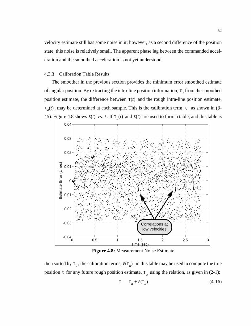
52
velocity estimate still has some noise in it; however, as a second difference of the position
state, this noise is relatively small. The apparent phase lag between the commanded accel-
eration and the smoothed acceleration is not yet understood.
4.3.3 Calibration Table Results
The smoother in the previous section provides the minimum error smoothed estimate
of angular position. By extracting the intra-line position information, , from the smoothed
position estimate, the difference between and the rough intra-line position estimate,
, may be determined at each sample. This is the calibration term, , as shown in (3-
45). Figure 4.8 shows vs. . If and are used to form a table, and this table is
then sorted by , the calibration terms, , in this table may be used to compute the true
position for any future rough position estimate, using the relation, as given in (2-1):
. (4-16)
τ
τ t( )
τa t( ) ε
0 0.5 1 1.5 2 2.5 3-0.04
-0.03
-0.02
-0.01
0
0.01
0.02
0.03
0.04
Time (sec)
Est
imate
Err
or
(Lin
es)
Figure 4.8:Measurement Noise Estimate
Correlations atlow velocities
ε t( ) t τa t( ) ε t( )
τa ε τa( )
τ τa
τ τa ε τa( )+=

53
It is interesting to note the apparent distribution of in Figure 4.8 above. Since the
Kalman filters use as a position measurement, is the “noise” in the signal. In
Section 3.3.1 it was noted that the Kalman filter assumes that the measurement noise has
low correlation between samples. This plot shows that this assumption is reasonably accu-
rate for this signal. The small sections where the plot looks time-correlated occur when the
velocity is near zero. These sections must be removed before the data is used to generate a
lookup table.
Figure 4.9 shows the contents of the raw sorted table computed from the data shown in
Figure 4.8. Note the general shape of the curve and the highly divergent regions pointed out
by the arrows in the figure. These regions occur because the filter estimate becomes inac-
curate when the measurement noise (i.e., ) becomes time-correlated due to low
velocities. These data are filtered out of the table using the magnitude of the smoothed es-
timate of the second state (velocity) as the criteria function. If all points with speed (i.e.,
ε t( )
τa ε t( ) τa
-0.5 -0.4 -0.3 -0.2 -0.1 0 0.1 0.2 0.3 0.4 0.5-0.03
-0.02
-0.01
0
0.01
0.02
0.03
(Lin
es)
ετ a
()
(Lines)τa
Figure 4.9:Raw Calibration Table
Errors due tolow velocities
ε t( )
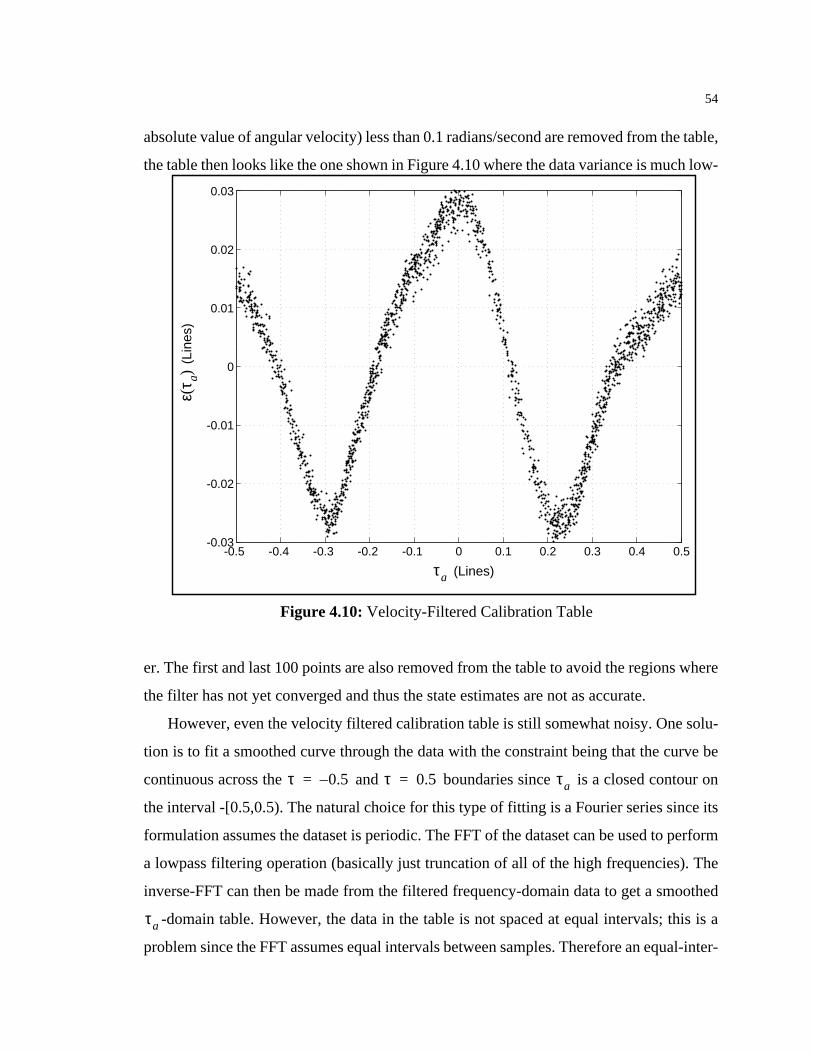
54
absolute value of angular velocity) less than 0.1 radians/second are removed from the table,
the table then looks like the one shown in Figure 4.10 where the data variance is much low-
er. The first and last 100 points are also removed from the table to avoid the regions where
the filter has not yet converged and thus the state estimates are not as accurate.
However, even the velocity filtered calibration table is still somewhat noisy. One solu-
tion is to fit a smoothed curve through the data with the constraint being that the curve be
continuous across the and boundaries since is a closed contour on
the interval -[0.5,0.5). The natural choice for this type of fitting is a Fourier series since its
formulation assumes the dataset is periodic. The FFT of the dataset can be used to perform
a lowpass filtering operation (basically just truncation of all of the high frequencies). The
inverse-FFT can then be made from the filtered frequency-domain data to get a smoothed
-domain table. However, the data in the table is not spaced at equal intervals; this is a
problem since the FFT assumes equal intervals between samples. Therefore an equal-inter-
-0.5 -0.4 -0.3 -0.2 -0.1 0 0.1 0.2 0.3 0.4 0.5-0.03
-0.02
-0.01
0
0.01
0.02
0.03
Figure 4.10:Velocity-Filtered Calibration Table
(Lines)τa
(Lin
es)
ετ a
()
τ 0.5–= τ 0.5= τa
τa
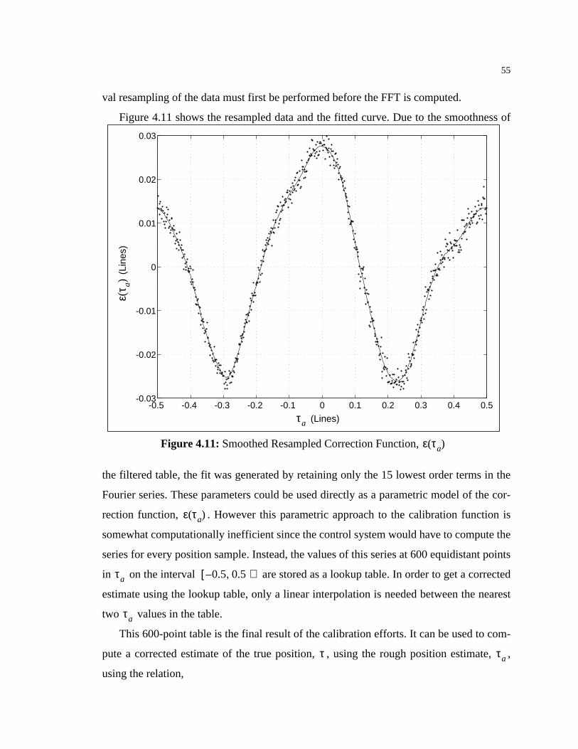
55
val resampling of the data must first be performed before the FFT is computed.
Figure 4.11 shows the resampled data and the fitted curve. Due to the smoothness of
the filtered table, the fit was generated by retaining only the 15 lowest order terms in the
Fourier series. These parameters could be used directly as a parametric model of the cor-
rection function, . However this parametric approach to the calibration function is
somewhat computationally inefficient since the control system would have to compute the
series for every position sample. Instead, the values of this series at 600 equidistant points
in on the interval are stored as a lookup table. In order to get a corrected
estimate using the lookup table, only a linear interpolation is needed between the nearest
two values in the table.
This 600-point table is the final result of the calibration efforts. It can be used to com-
pute a corrected estimate of the true position, , using the rough position estimate, ,
using the relation,
-0.5 -0.4 -0.3 -0.2 -0.1 0 0.1 0.2 0.3 0.4 0.5-0.03
-0.02
-0.01
0
0.01
0.02
0.03
Figure 4.11:Smoothed Resampled Correction Function,ε τa( )
(Lines)τa
(Lin
es)
ετ a
()
ε τa( )
τa 0.5 0.5, )–[
τa
τ τa

56
. (4-17)
Linear interpolation into the lookup table is used to determine the actual value for
when does not fall exactly on one of the table elements.
4.3.4 Algorithm Implementation
The experimental algorithm was implemented in aMATLAB function. The full MAT-
LAB implementation can be seen in Appendix B. The function is called with the rough state
estimates, , and the motor current commands, , as input vectors and returns a lookup
table as a array where the first row contains the table index ( ) and the second
row contains the associated correction factor, .
τ t( ) τa t( )= ε τa( )+
ε τa( )
τa
xr im
2 600× τa
ε τa( )

CHAPTER 5: EXPERIMENTAL RESULTS
The previous chapter showed the derivation of a calibration table using experimental
data. The validity of this table should be verified under experimental conditions so that the
performance of this table-based correction of the rough position estimate may be evaluated.
5.1 Off-line Comparison
The calibration table is generated from data taken from a physically operational system.
One way to verify this calibration is to use the original, rough intra-line position estimates,
, and the calibration terms from the new calibration table, , to compute the correct-
ed position estimates. These corrected position estimates and their derivatives may then be
compared to the smoothed state estimates generated by the Kalman filter/smoother during
the calibration process.
The top and bottom graphs in Figure 5.1 show the difference between the smoothed po-
sition estimate and the rough position estimate, , before and after it has been corrected
by the calibration lookup table. The periodic large spikes in the corrected position error are
due to the position estimate errors in the Kalman filter induced by measurement noise cor-
relation at low velocities. The plot shows that the rough position estimate varies by
of a line from the correct position (assuming that the smoothed position estimate is really
correct). The corrected position estimate varies by of a line, a factor of 7.5 increase
in precision over the rough position estimate. Thus, for the experimental setup, the correct-
ed position estimate improves the digital encoder precision of line by a factor of
62.5(~6.0 bits compared to the rough position estimate’s improvement by a factor of only
8.3(~3.0 bits).
Another method of comparing the measurement is by examining the velocity as com-
puted by the first difference of position. Figure 5.2 shows the velocity estimate from the
Kalman filter/smoother, overlaid by the first-difference of the rough position estimates and
the first-difference of the corrected position estimates. The plot shows that the velocity es-
timates based on the corrected rough intra-line position, (i.e., ) are much closer to
the underlying Kalman filter/smoother velocity estimate. These velocity estimates provide
an important qualitative measure of improvement because typical control algorithms such
τa ε τa( )
τa
0.03±
0.004±
0.25±
τa ε τa( )+

58
1 1.2 1.4 1.6 1.8 2 2.2 2.4 2.6 2.8-0.05
-0.04
-0.03
-0.02
-0.01
0
0.01
0.02
0.03
0.04
0.05
Time (sec)
Rou
gh P
ositi
on--
Res
idua
l Err
or (
Line
s)
1 1.2 1.4 1.6 1.8 2 2.2 2.4 2.6 2.8-0.05
-0.04
-0.03
-0.02
-0.01
0
0.01
0.02
0.03
0.04
0.05
Time (sec)
Cor
rect
ed P
ositi
on--
Res
idua
l Err
or (
Line
s)
Figure 5.1:Position Error Residuals Before and After Correction
Position Error Residual Before Correction
Position Error Residual After Correction

59
as the PID algorithm use the velocity (as computed by the first difference of position) as a
control input. If the velocity estimate is noisy, it will induce significant disturbances to the
control system.
5.2 Physical Verification
The previously described calibration method may be verified by direct physical mea-
surements. If the encoder signals are sampled at known intra-line positions , then may
be computed from the sampled signals using
(5-1)
and the calibration terms may be computed using
. (5-2)
The challenge with this approach to calibration is that high line-count encoders will require
very high-precision angular measurements to obtain accurate estimates of . These mea-
0.85 0.9 0.95 1 1.05 1.1
-0.14
-0.12
-0.1
-0.08
-0.06
-0.04
-0.02
0
Time (sec)
Vel
ocity
(lin
es/s
amp)
Figure 5.2:Velocity Estimate Comparison
Velocity estimateusing uncorrected
τa
Velocity estimateusing table-
τacorrected
τ τa
τa2 b a,( )atan2π
------------------------------=
ε τa( ) τ τa–=
τa

60
surements may be difficult and/or expensive to obtain.
5.2.1 Physical Calibration Setup
The physical calibration setup for the experimental system is shown in Figure 5-3. A
linear motion stage is used to control angular displacement of the robot joint. Since the 12-
bit A/D converters are theoretically capable of resolving down to
of a line, the 152mm link length joint would require linear position precisions of
(5-3)
at the end of the robot link. A steel rod is used to extend the radius of rotation for this joint
to about 690mm. This decreases the linear position precision requirements at the end of the
rod to . At this radius, a linear motion range of
(5-4)
is needed to scan one encoder line. Only a laser interferometer has the linear motion preci-
sion necessary to resolve the increments implied by (5-3). Since no interferometer
was immediately available, a -precision linear micrometer stage was used at the ex-
pense of some lost calibration precision. Even at this resolution, special care had to be taken
to allow the motions to occur at a constant radius of rotation. Since the distance measure-
ControlKnob
Robot Jointwith Encoder
~690mm
RollerBearing
Mic
rom
eter
Figure 5.3:Physical Calibration Setup
δτ 1 212⁄ 0.0002==
∆y r2πNl------ ∆τ⋅
sin=
152mm2π Radians( )1000 Lines( )--------------------------------- 0.0002 Lines( )⋅sin⋅
=
0.19µm=
0.87µm
y r θsin 690mm2π Radians( )1000 Lines( )---------------------------------sin⋅ 4.34mm= = =
190nm
10µm
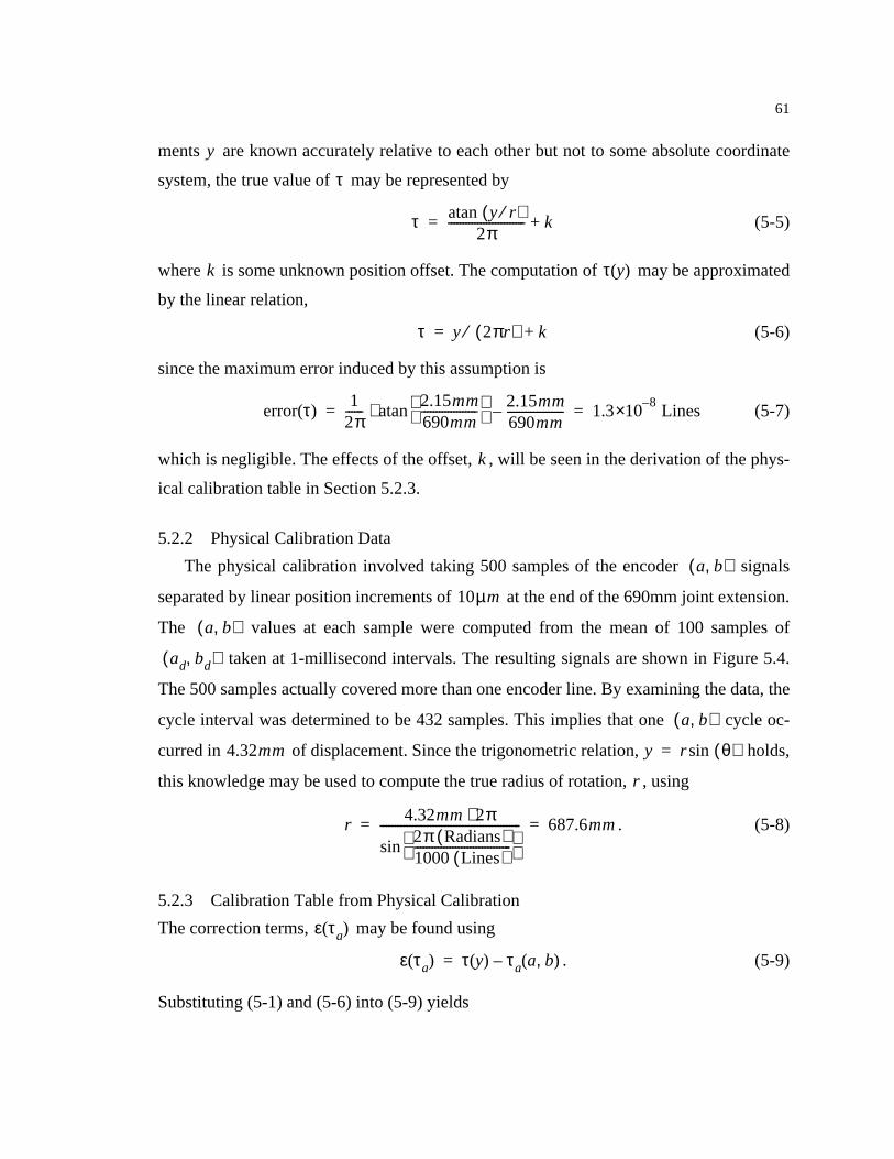
61
ments are known accurately relative to each other but not to some absolute coordinate
system, the true value of may be represented by
(5-5)
where is some unknown position offset. The computation of may be approximated
by the linear relation,
(5-6)
since the maximum error induced by this assumption is
(5-7)
which is negligible. The effects of the offset, , will be seen in the derivation of the phys-
ical calibration table in Section 5.2.3.
5.2.2 Physical Calibration Data
The physical calibration involved taking 500 samples of the encoder signals
separated by linear position increments of at the end of the 690mm joint extension.
The values at each sample were computed from the mean of 100 samples of
taken at 1-millisecond intervals. The resulting signals are shown in Figure 5.4.
The 500 samples actually covered more than one encoder line. By examining the data, the
cycle interval was determined to be 432 samples. This implies that one cycle oc-
curred in of displacement. Since the trigonometric relation, holds,
this knowledge may be used to compute the true radius of rotation, , using
. (5-8)
5.2.3 Calibration Table from Physical Calibration
The correction terms, may be found using
. (5-9)
Substituting (5-1) and (5-6) into (5-9) yields
y
τ
τ y r⁄( )atan2π
-------------------------- k+=
k τ y( )
τ y 2πr( )⁄ k+=
error τ( )1
2π------ 2.15mm
690mm-------------------
atan 2.15mm690mm-------------------–⋅ 1.3
8–×10 Lines= =
k
a b,( )
10µm
a b,( )
ad bd,( )
a b,( )
4.32mm y r θ( )sin=
r
r4.32mm 2π⋅2π Radians( )1000 Lines( )---------------------------------
sin------------------------------------------------ 687.6mm= =
ε τa( )
ε τa( ) τ y( ) τa a b,( )–=

62
. (5-10)
The calibration terms, , may be sorted by to form a physical calibration table. Fig-
ure 5.5 shows the calibration table generated by this physical calibration method. Note the
constant, , in (5-10) causes an unknown offset constant offset in the physical calibration
table. This offset must be determined before the physical calibration table can be compared
to the calibration table generated by the Kalman filter/smoother.
5.2.4 Comparison of Physical Calibration to Kalman Calibration
Figure 5.6 shows the results of this calibration table overlaid with the calibration table
from the Kalman filter approach. The plot shows that the two calibration methods have only
slight differences in phase and amplitude as a function of . The worst-case error (resid-
ual) in is about 0.005 lines. If the physical calibration is assumed to be correct, then
the 0.005 residual is the worst-case correction error from the Kalman calibration method.
0 0.5 1 1.5 2 2.5 3 3.5 4 4.5 5-2000
-1500
-1000
-500
0
500
1000
1500
2000
y-Displacement (mm)
(a,b
) va
lues
(A
/D U
nits
)
Figure 5.4:Physical Calibration Data: (a,b) Values vs. Displacement
ε τa( ) y2πr--------- k
2 b a,( )atan2π
------------------------------–+=
ε τa( ) τa
k
τa
ε τa( )

63
This corresponds to a resolution of 1/200th of an encoder line, a factor of 50 improvement
over the 0.25-line digital resolution.
The Kalman calibration and physical calibrations leading to the plots in Figure 5.6 were
performed again after disassembly and reassembly of the encoder. Figure 5.7 shows this
new calibration comparison. Note that while the shape of the calibration table is very dif-
ferent (e.g., it has four peaks instead of two), the Kalman calibration and the physical
calibration are still in very close agreement with the worst case residual error between the
two methods of about 0.007 lines.
5.2.5 Relative Precision of Physical and Kalman Calibration
In Section 5.2.1, it was shown that the necessary linear positioning resolution to resolve
0.0002 of a line was . Since the micrometers have resolution, preci-
sion is assumed. The corresponding intra-line precision may be solved using (5-3) rewritten
in terms of :
-0.5 -0.4 -0.3 -0.2 -0.1 0 0.1 0.2 0.3 0.4 0.5-0.03
-0.02
-0.01
0
0.01
0.02
0.03
0.04
0.05
0.06
0.07
Tau_a (Lines
Tau
- T
au_a
(Li
nes)
Figure 5.5:Calibration Table from Physical Calibration
0.19µm 10µm 5µm±
∆τ

64
. (5-11)
Therefore, the precision of the physically measured intra-line position is only slightly
smaller than the worst-case residual error seen in Figure 5.6. This implies that a more pre-
cise position measurement scheme is needed to determine the accuracy of the Kalman cal-
ibration technique.
One qualitative measure of a calibration table accuracy is the smoothness of the veloc-
ity estimate of a moving system as computed from first-difference of the corrected position
estimates. Figure 5.2 shows this velocity estimate as extracted from position estimates that
have been corrected using the Kalman calibration table. Figure 5.8 shows the velocity es-
timate for the same dataset using a calibration table derived from the physical calibration.
-0.5 -0.4 -0.3 -0.2 -0.1 0 0.1 0.2 0.3 0.4 0.5-0.05
-0.04
-0.03
-0.02
-0.01
0
0.01
0.02
0.03
0.04
0.05
Tau_a (Lines)
Cal
ibra
tion
Ter
m: T
au -
Tau
_a (
Line
s)
Figure 5.6:Comparison of Kalman Calibration with Physical Calibration
KalmanCalibration
Data
PhysicalCalibration
Data
∆τNL
2π------ ∆y
r------
asin⋅=
1000 Lines( )2π Radians( )--------------------------------- 0.005mm±
687.6mm--------------------------
asin⋅=
0.0012 Lines( )±=
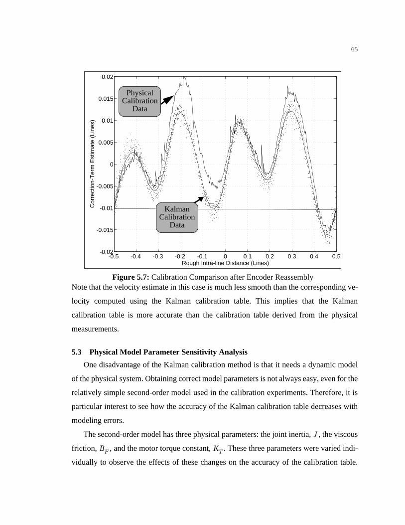
65
Note that the velocity estimate in this case is much less smooth than the corresponding ve-
locity computed using the Kalman calibration table. This implies that the Kalman
calibration table is more accurate than the calibration table derived from the physical
measurements.
5.3 Physical Model Parameter Sensitivity Analysis
One disadvantage of the Kalman calibration method is that it needs a dynamic model
of the physical system. Obtaining correct model parameters is not always easy, even for the
relatively simple second-order model used in the calibration experiments. Therefore, it is
particular interest to see how the accuracy of the Kalman calibration table decreases with
modeling errors.
The second-order model has three physical parameters: the joint inertia, , the viscous
friction, , and the motor torque constant, . These three parameters were varied indi-
vidually to observe the effects of these changes on the accuracy of the calibration table.
-0.5 -0.4 -0.3 -0.2 -0.1 0 0.1 0.2 0.3 0.4 0.5-0.02
-0.015
-0.01
-0.005
0
0.005
0.01
0.015
0.02
Rough Intra-line Distance (Lines)
Cor
rect
ion-
Ter
m E
stim
ate
(Lin
es)
Figure 5.7:Calibration Comparison after Encoder Reassembly
PhysicalCalibration
Data
KalmanCalibration
Data
J
BF KT

66
Figure 5.9, Figure 5.10, and Figure 5.11 show the changes in the nominal calibration table
(i.e., the table derived from the correct physical parameters) for a variety of values of ,
, and respectively. These three plots show that the error in the calibration table in-
duced by any one these physical model parameter errors is less than 0.01 lines. This is still
a factor of 3 better than the rough position estimate (see Figure 4.8 on page 52).
0.85 0.9 0.95 1 1.05 1.1
-0.14
-0.12
-0.1
-0.08
-0.06
-0.04
-0.02
0
Time (sec)
Vel
ocity
(lin
es/s
amp)
Figure 5.8:Velocity Estimate from Physical Calibration Table
J
BF KT
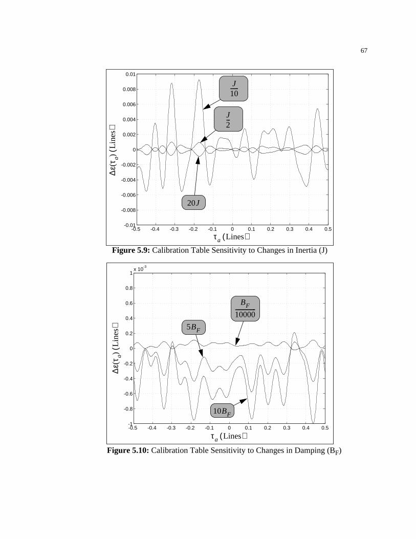
67
-0.5 -0.4 -0.3 -0.2 -0.1 0 0.1 0.2 0.3 0.4 0.5-0.01
-0.008
-0.006
-0.004
-0.002
0
0.002
0.004
0.006
0.008
0.01
Figure 5.9:Calibration Table Sensitivity to Changes in Inertia (J)
τa Lines( )
∆ε
τ a(
)Li
nes
()
J10------
J2---
20J
-0.5 -0.4 -0.3 -0.2 -0.1 0 0.1 0.2 0.3 0.4 0.5-1
-0.8
-0.6
-0.4
-0.2
0
0.2
0.4
0.6
0.8
1x 10
-3
∆ε
τ a(
)Li
nes
()
τa Lines( )
Figure 5.10:Calibration Table Sensitivity to Changes in Damping (BF)
10BF
5BF
BF
10000---------------

68
-0.5 -0.4 -0.3 -0.2 -0.1 0 0.1 0.2 0.3 0.4 0.5-0.01
-0.008
-0.006
-0.004
-0.002
0
0.002
0.004
0.006
0.008
0.01
∆ε
τ a(
)Li
nes
()
τa Lines( )
Figure 5.11:Calibration Table Sensitivity to Changes in Torque Constant (KT)
KT
100---------
5KT
10KT

CHAPTER 6: CONCLUSIONS
6.1 Summary of work
An off-line method for generating a calibration table for an analog position encoder has
been presented. The method employs a Kalman filter/smoother to estimate true intra-line
position, , of the encoder based on the rough position estimate, , and a dynamic model
of the encoder/actuator system including a deterministic commanded current input. The
difference between the Kalman filter/smoother estimate of position and the rough position
estimate is used to generate the calibration table of correction terms, .
A mathematical derivation of the variance of the estimated intra-line position as a func-
tion of the encoder signal variances and the output values was derived in Chapter 2. This
derivation showed that, for the experimental system, the measurement noise from the en-
coders imposes a resolution limitation of about 0.001 of a line.
An experimental implementation of this calibration method was done using a 1000-line
analog quadrature rotary encoder. A physical calibration experiment using a -reso-
lution micrometer indicates that the Kalman calibration method agrees with the physical
calibration to at least 0.005-line intra-line interpolation precision. Qualitative comparisons
between the Kalman calibration results and the physical calibration (Section 5.2.5) indicate
that the Kalman calibration method is more accurate than the physical calibration; however,
a more precise physical calibration using a laser interferometer is needed to verify this
claim quantitatively.
6.2 Advantages of the Kalman Calibration Method
The Kalman calibration method allows an encoder to be calibrated on an installed sys-
tem without the need for external precision calibration hardware such as micrometers or
laser interferometers. This is an important feature for many encoders which suffer signifi-
cant changes in their calibration tables after removal and re-installation on a given system.
Additionally, it is often not feasible to make a physical calibration using external devices
due to space and time constraints.
Unlike the parametric calibration method in [2] (which assumes that the encoder out-
puts functions and are sinusoidal), the Kalman calibration method is applicable
τ τa
ε τa( )
10µm
a τ( ) b τ( )

70
to a wide variety of encoder output functions which may not fit a parametric model. Both
the constant velocity calibration method [3] and the Kalman calibration method generate a
calibration table which can be used to estimate true intra-line position, , from an ideal in-
tra-line position, , using the relation,
(5-12)
and is the correction term from the calibration table for a given . However, unlike
the constant velocity method, this calibration method does not require constant velocity
motion during the calibration process (which is difficult to obtain). Instead, the method
works best withchanging velocities, which is much easier to obtain. In addition, the con-
stant velocity calibration method requires very high-speed (for example, 100-kHz) sam-
pling of the encoder signals, while the Kalman calibration method may be used with the
normal operational sampling rate of the embedded control system (for example, 1-kHz).
6.3 Future Directions
6.3.1 Improved Verification of Calibration Precision
The current experimental results indicate that the Kalman calibration method yields in-
tra-line position estimates that are at least as precise as the physical calibration setup used
to verify its precision. A more accurate physical calibration method is needed using a laser
interferometer to verify the accuracy of this Kalman calibration method.
The Kalman calibration method, as currently derived, implicitly assumes that the en-
coder output signals, and are identical for all adjacent line pairs on the encoder
disk. A laser interferometer could be used to get a better estimate of these differences. If
significant, the Kalman calibration method could be reformulated to generate separate cal-
ibration tables for each adjacent line-pair on the encoder disk, although this may
substantially increase the storage requirements for the calibration table. More extensive ex-
perimentation with a wider range of analog quadrature position encoders is needed to gain
more knowledge of how prevalent this adjacent line-pair variance problem may be.
τ
τa
τ τa ε τa( )+= whereτa2 b a,( )atan2π
------------------------------=
ε τa( ) τa
a τ( ) b τ( )

71
6.3.2 Improved Noise Modeling
The bottom plot in Figure 5.1 shows a slight periodicity in the residual error of the cor-
rected rough position estimates over time. This indicates that the Kalman filter/smoother
estimates may be improved if a more accurate model of the measurement noise is known.
Correlations of this noise are known to become significant, as shown in Figure 4.8, at lower
magnitude velocities. It may be that even at higher velocities, the slight coloration of this
noise is affecting the filter performance. Gelb, et.al. [12], showed that the DGMP model
can be augmented to incorporate colored measurement noise by adding states which act as
first-order systems forced by white noise inputs. This type of augmentation may improve
the Kalman filter/smoother estimation performance.
6.3.3 Embedded System Implementation
The current Kalman calibration algorithm is implemented in MATLAB. The algorithm
can be reformulated in a high-level programming language such asC and implemented on
an embedded control system. Calibration could then be done at any time with several sec-
onds of computational time on more powerful control system architectures such as the
DSP-based controller used in the experimental system discussed in Chapter 4. It may be
possible to formulate the calibration process to run as a background process on the control-
ler which updates the calibration table based on observing the sensor signals and
commanded outputs of the real-time control system during operations.

REFERENCES
[1] Hewlett Packard Components Group, “Quadrature Decoder/Counter Interface IC,”Optoelectronics Designer’s Catalog, Hewlett Packard Corp., pp. 1-61 through 1-76,1992.
[2] P.H. Marbot, “Mini Direct Drive Robot for Biomedical Applications,” MSEE Mas-ter’s Thesis, Biorobotics Laboratory, University of Washington, Seattle, 1992.
[3] N. Hagiwara, Y. Suzuki, H. Murase, “A Method of Improving the Resolution and Ac-curacy of Rotary Encoders Using a Code Compensation Technique,” IEEETransactions on Instrumentation and Measurement, Vol. 41, No. 1, pp. 98-101, Feb-ruary, 1992.
[4] J.P. Karidis, et.al., “The Hummingbird Minipositioner—Providing Three-Axis Mo-tion at 50 G’s With Low Reactions,” Proceedings of the IEEE InternationalConference on Robotics and Automation, pp. 685-692, Nice, France, May, 1992.
[5] B.A. Sawyer, US Patent No3,457,482, July 1969.
[6] J. Ish-Shalom, “Sawyer Sensor for Planar Motion Systems,” Proceedings of the IEEEInternational Conference on Robotics and Automation, Vol. 3, pp. 2652-2658, SanDiego, May, 1994.
[7] B. Hannaford, P.H. Marbot, M. Moreyra, S. Venema, “A 5-Axis Mini Direct DriveRobot for Time Delayed Teleoperation,” To be published in Proceedings of IROS,Munich, September, 1994.
[8] M.R. Moreyra, “Design of a Five Degree of Freedom Direct Drive Mini-robot usingDisk Drive Actuators,” MSME Master’s Thesis, Biorobotics Laboratory, Universityof Washington, Seattle, 1994.
[9] I. MacDuff, S. Venema, B. Hannaford, “The Anthroform Neural Controller: A Sys-tem for Detailed Emulation of Neural Circuits,” Proceedings of IEEE InternationalConference on System’s, Man, and Cybernetics, Vol. 1, pp. 117-122, Chicago, 1992.
[10] A. Leon-Garcia, “Probability and Random Processes for Electrical Engineering,” Ad-dison-Wesley, pp. 233-236, 1989.
[11] R.E. Kalman, “A New Approach to Linear Filtering and Prediction Problems,” Jour-nal of Basic Engineering (ASME), 82D, pp. 35-45, March, 1960.
[12] A. Gelb, et.al., “Applied Optimal Estimation,” Analytic Sciences Corporation, M.I.T.Press, pp. 182-203, 1988.
73
[13] C.F. Van Loan, “Computing Integrals Involving the Matrix Exponential,” IEEETransactions on Automatic Control, Vol. AC-23, No. 3, pp. 395-404, June 1978.
[14] A.E. Bryson, Jr., “Dynamic Optimization with Uncertainty,” Pre-publication draft,Stanford University, March, 1993.
[15] A.E. Bryson and M. Frazier, “Smoothing for Linear and Nonlinear Dynamic Sys-tems,” Technical Report, ASD-TDR-63-119, pp. 496-503, Wright Patterson AirForce Base, Ohio, September, 1962.

APPENDIX A: VAN-LOAN ALGORITHM REVIEW
Van Loan’s algorithm defines a matrix, , whose elements are several sub-matrices:
. (A-1)
where is the interval of integration, are real matrices of dimensions
respectively, and is symmetric positive semidefinite. The matrix,
, is defined as the matrix exponential of and is used to compute a new set of sub-ma-
trices:
. (A-2)
Using these relational definitions for and , Van Loan showed that the following rela-
tions hold true for the sub-matrices of and as defined above:
(A-3)
By comparing (3-15) through (3-17) to (A-3), the first integral in (A-3) is identical in
C
C
AT
– I 0 0
0 AT
– D 0
0 0 A B
0 0 0 0
=∆
∆ A B D, ,[ ]
n n n p n n×,×,×[ ] D
S C
S Ct( )exp
F1 G1 H1 K1
0 F2 G2 H2
0 0 F3 G3
0 0 0 F4
==∆
C S
C S
H ∆( ) As( )exp B sd
0
∆
∫= G3 ∆( )=
Q ∆( ) ATs
exp D As( )exp sd
0
∆
∫= F3 ∆( )TG2 ∆( )=
M ∆( ) ATs
exp DH s( ) sd
0
∆
∫= F3 ∆( )TH2 ∆( )=
W ∆( ) H s( )TDH s( )ds
0
∆
∫= BF3 ∆( )TK1 ∆( ) B
TF3 ∆( )
TK1 ∆( )
T+=

75
form to the integrals needed to compute (3-15) and (3-16), while the second integral in (A-
3) is identical in form to (3-17). In addition, it can be shown [14] that the relation,
(A-4)
holds true, allowing the computation of (3-14) as well. Therefore the following assign-
ments are made to compute these integrals:
, (A-5)
, (A-6)
, (A-7)
and
(A-8)
which allows to be computed as follows:
(A-9)
From the definitions, the discrete system parameters are extracted from :
(A-10)
(A-11)
(A-12)
At( )exp F3 ∆( )=
A AT
=
B I=
D BQBT=
Ts ∆=
S
S
AT
– I 0 0
0 AT
– ΓcQΓcT
0
0 0 A I
0 0 0 0
t
exp=
S
Φ F3T S55 S56
S65 S66
= =
Ψ G3TB
S57 S58
S67 S68
B= =
Γ G3TΓc
S57 S58
S67 S68
Γc= =

76
. (A-13)W F3TG2
S55 S56
S65 S66
S35 S36
S45 S46
= =
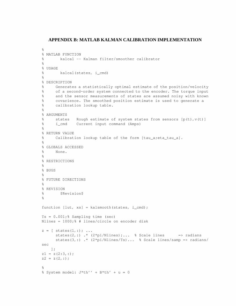
APPENDIX B: MATLAB KALMAN CALIBRATION IMPLEMENTATION
%% MATLAB FUNCTION% kalcal -- Kalman filter/smoother calibrator%% USAGE% kalcal(states, i_cmd)%% DESCRIPTION% Generates a statistically optimal estimate of the position/velocity% of a second-order system connected to the encoder. The torque input% and the sensor measurements of states are assumed noisy with known% covarience. The smoothed position estimate is used to generate a% calibration lookup table.%% ARGUMENTS% states Rough estimate of system states from sensors [p(t),v(t)]% i_cmd Current input command (Amps)%% RETURN VALUE% Calibration lookup table of the form [tau_a;eta_tau_a].%% GLOBALS ACCESSED% None.%% RESTRICTIONS%% BUGS%% FUTURE DIRECTIONS%% REVISION% $Revision$%
function [lut, xs] = kalsmooth(states, i_cmd);
Ts = 0.001;% Sampling time (sec)Nlines = 1000;% # lines/circle on encoder disk
z = [ states(1,:); ...states(2,:) .* (2*pi/Nlines);... % Scale lines => radiansstates(3,:) .* (2*pi/Nlines/Ts)... % Scale lines/samp => radians/
sec ];z1 = z(2:3,:);z2 = z(2,:);
%% System model: J*th’’ + B*th’ + u = 0

78
% where th is angular position (theta)% J is rotational inertia% B is viscous friction% u is torque input (from actuator)%
%% System parameters%Bf = 1e-3% System viscous friction [ Nm/(rad/sec^2) => Kg*m^2 ]J = 0.000916% System rotational inertia [Nm/(rad/sec) => Kg*m^2/sec ]Km = 0.053% Motor torque constant (Nm/A) [Determined experimentally]V = 8.88e-9% measurement noise variance (0.015-line^2, => rad^2)Q = 1e-2% Spectral Density of process noisep_hat0 = [5e-9, 0.0;% Initial state covariance
0.0, 1e-4]
%% Continuous 2nd-order system parameters%Ac = [0,1,;0,-Bf/J]% Cont-time state transition matrixBc = [0;-Km/J] % Cont-time cmd input distributionGc = [0;1] % Cont-time process noise distribution
C_hat = [ -Ac, eye(2,2), zeros(2,2), zeros(2,2);... zeros(2,2), -Ac, Gc*Q*Gc’, zeros(2,2);... zeros(2,2), zeros(2,2), Ac’, eye(2,2);... zeros(2,2), zeros(2,2), zeros(2,2), zeros(2,2) ];
S_hat = expm(C_hat .* Ts);
Phi = S_hat(5:6,5:6)’% State transition matrixPsi = S_hat(5:6,7:8)’ * Bc% Cmd input distributionCd = [1,0] % Sensor input distribution (radians)Gd = S_hat(5:6,7:8)’ * Gc% Process noise distributionW = S_hat(5:6,5:6)’ * S_hat(3:4,5:6)% Process noise covariance
%% Assume that the sensor data is in matrix z(nsensors,nsamples).% Guess at the initial state and initial state variance%nstates = 2; % Number of process statesninputs = 1; % Number of process inputsnsensors = 1; % Number of sensor outputsnsamps = size(z,2);% Number of sensor samplesvel0_guess = mean(z1(2,1:10));velK_guess = mean(z1(2,nsamps-10:nsamps));x_hat0 = [z2(:,1);vel0_guess]% Initial state estimatex_hatK = [z2(:,nsamps);velK_guess]% Final state estimate
fprintf(2,’\n’);

79
fprintf(2,’\t*******************************************\n’);fprintf(2,’\t************Starting FWD Filter************\n’);fprintf(2,’\t*******************************************\n’);
%% Initialize the output matricies for speed%xf_bar= zeros(nstates,nsamps);xb_bar= zeros(nstates,nsamps);xf_hat= zeros(nstates,nsamps);xb_hat= zeros(nstates,nsamps);pf = zeros(nstates,nsamps*nstates);pb = zeros(nstates,nsamps*nstates);ps = zeros(nstates,nsamps*nstates);kf = zeros(nstates,nsamps);kb = zeros(nstates,nsamps);ks = zeros(nstates,nsamps);
%% Do forward filter%xf_hat(:,1) = x_hat0;xf_bar(:,1) = x_hat0;p_hat = p_hat0;pf(:,1:2) = p_hat0;tile_ndx = 3;for ndx = 2:nsamps,
%% Time update%xf_bar(:,ndx) = Phi * xf_hat(:,ndx-1) + Psi * i_cmd(ndx);p_bar = Phi * p_hat * Phi’ + W;
%% Measurement update%tmp = V + Cd * p_bar * Cd’;% common sub-expressionk_gain = p_bar * Cd’ * inv(tmp);p_hat = p_bar - k_gain * tmp * k_gain’;xf_hat(:,ndx) = xf_bar(:,ndx) ...
+ k_gain * ( z2(ndx) - Cd * xf_bar(:,ndx) );
pf(:,tile_ndx:tile_ndx+1) = p_hat;kf(:,ndx) = k_gain;tile_ndx = tile_ndx + nstates;
end
%% Estimate acceleration from 1st difference of estimate velocity%acc1 = diff(xf_bar(2,:));

80
acc2 = diff(xf_hat(2,:));
p_barp_hatk_gain
%% Plot out forward filter results%figure(1)clfsubplot(221)plot(z(1,:),z(2,:),’r-’,z(1,:),xf_hat(1,:)’,’y-’);xlabel(‘Time (sec)’)ylabel(‘xf_hat(1,:) -> pos (rad)’)gridsubplot(222)plot(z(1,:),z(2,:)-xf_hat(1,:),’r.’)xlabel(‘Time (sec)’)ylabel(‘xf_hat[bar](:,1) - atan’)gridsubplot(223)plot(z(1,:),z(3,:),’r.’,z(1,:),xf_hat(2,:)’,’y-’);xlabel(‘Time (sec)’)ylabel(‘xf_hat(2,:) -> vel (rad/sec)’)gridsubplot(224)plot(z(1,2:nsamps),acc2,’y.’,z(1,:),Psi(2,1)*i_cmd,’r-’)xlabel(‘Time (sec)’)ylabel(‘Est Acceleration (rad/sec^2)’)griddrawnow
%% Extract forward filter covariances (state1^2, state2^2)%pf4plot = zeros(2,nsamps);tile_ndx = 1;for ndx = 1:nsamps,
%% Get covariance for first state (position)%pf4plot(1,ndx) = pf(1,tile_ndx);pf4plot(2,ndx) = pf(2,tile_ndx+1);tile_ndx = tile_ndx + nstates;
end%% Plot forward filter covariances%figure(2)clf

81
subplot(221);plot(z(1,:),pf4plot(1,:),’y-’);xlabel(‘Time (sec)’)ylabel(‘Fwd Position Covariance’)gridsubplot(223);plot(z(1,:),pf4plot(2,:),’y-’);xlabel(‘Time (sec)’)ylabel(‘Fwd Velocity Covariance’)gridsubplot(222);plot(z(1,:),kf(1,:),’y-’);xlabel(‘Time (sec)’)ylabel(‘Fwd Position Gain’)gridsubplot(224);plot(z(1,:),kf(2,:),’y-’);xlabel(‘Time (sec)’)ylabel(‘Fwd Velocity Gain’)gridfprintf(2,’FWD filter done. Press any character to continue...’);pausefprintf(2,’\n’);fprintf(2,’\t*******************************************\n’);fprintf(2,’\t***********Starting BKWD Filter************\n’);fprintf(2,’\t*******************************************\n’);
%% Do backward filter%xb_hat(:,nsamps) = x_hatK;xb_bar(:,nsamps) = x_hatK;Phi_inv = inv(Phi);p_bar = p_hat0;pb(:,2*nsamps-1:2*nsamps) = p_hat0;tile_ndx = 2*nsamps - 3;for ndx = nsamps-1:-1:1,
%% Time downdate%xb_hat(:,ndx) = Phi_inv * xb_bar(:,ndx+1)...
- Phi_inv * Psi * i_cmd(ndx);p_hat = Phi_inv * p_bar * Phi_inv’ + W;
%% Measurement downdate%tmp = V + Cd * p_hat * Cd’;% common sub-expressionk_gain = p_hat * Cd’ * inv(tmp);p_bar = p_hat - k_gain * tmp * k_gain’;xb_bar(:,ndx) = xb_hat(:,ndx)...
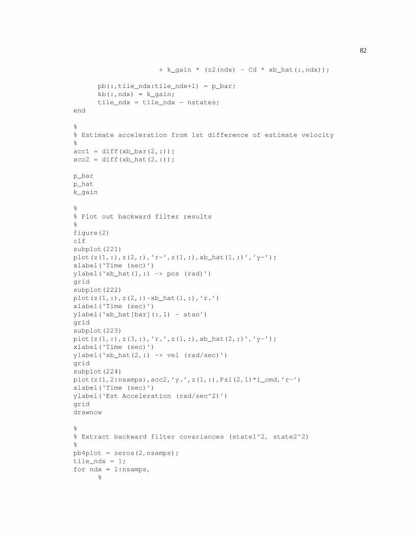
82
+ k_gain * (z2(ndx) - Cd * xb_hat(:,ndx));
pb(:,tile_ndx:tile_ndx+1) = p_bar;kb(:,ndx) = k_gain;tile_ndx = tile_ndx - nstates;
end
%% Estimate acceleration from 1st difference of estimate velocity%acc1 = diff(xb_bar(2,:));acc2 = diff(xb_hat(2,:));
p_barp_hatk_gain
%% Plot out backward filter results%figure(2)clfsubplot(221)plot(z(1,:),z(2,:),’r-’,z(1,:),xb_hat(1,:)’,’y-’);xlabel(‘Time (sec)’)ylabel(‘xb_hat(1,:) -> pos (rad)’)gridsubplot(222)plot(z(1,:),z(2,:)-xb_hat(1,:),’r.’)xlabel(‘Time (sec)’)ylabel(‘xb_hat[bar](:,1) - atan’)gridsubplot(223)plot(z(1,:),z(3,:),’r.’,z(1,:),xb_hat(2,:)’,’y-’);xlabel(‘Time (sec)’)ylabel(‘xb_hat(2,:) -> vel (rad/sec)’)gridsubplot(224)plot(z(1,2:nsamps),acc2,’y.’,z(1,:),Psi(2,1)*i_cmd,’r-’)xlabel(‘Time (sec)’)ylabel(‘Est Acceleration (rad/sec^2)’)griddrawnow
%% Extract backward filter covariances (state1^2, state2^2)%pb4plot = zeros(2,nsamps);tile_ndx = 1;for ndx = 1:nsamps,
%

83
% Get covariance for first state (position)%pb4plot(1,ndx) = pb(1,tile_ndx);pb4plot(2,ndx) = pb(2,tile_ndx+1);tile_ndx = tile_ndx + nstates;
end%% Plot backward filter covariances%figure(3)clfsubplot(221);plot(z(1,:),pb4plot(1,:),’y-’);xlabel(‘Time (sec)’)ylabel(‘Bkwd Position Covariance’)gridsubplot(223);plot(z(1,:),pb4plot(2,:),’y-’);xlabel(‘Time (sec)’)ylabel(‘Bkwd Velocity Covariance’)gridsubplot(222);plot(z(1,:),kb(1,:),’y-’);xlabel(‘Time (sec)’)ylabel(‘Bkwd Position Gain’)gridsubplot(224);plot(z(1,:),kb(2,:),’y-’);xlabel(‘Time (sec)’)ylabel(‘Bkwd Velocity Gain’)grid
fprintf(2,’BKWD filter done. Press any character to continue...’);pausefprintf(2,’\n’);fprintf(2,’\t*******************************************\n’);fprintf(2,’\t*************Starting Smoother*************\n’);fprintf(2,’\t*******************************************\n’);
%% Now generate the smoothed estimates%xs = zeros(nstates,nsamps);tile_ndx = 1;for ndx = 1:nsamps,
k_gain = pf(:,tile_ndx:tile_ndx+1) ... * inv(pf(:,tile_ndx:tile_ndx+1) + pb(:,tile_ndx:tile_ndx+1));xs(:,ndx) = xf_bar(:,ndx) + k_gain * (xb_bar(:,ndx) -
xf_bar(:,ndx));

84
ps(:,tile_ndx:tile_ndx+1) = pf(:,tile_ndx:tile_ndx+1) ... - k_gain * pf(:,tile_ndx:tile_ndx+1);
ks(:,tile_ndx:tile_ndx+1) = k_gain;tile_ndx = tile_ndx + nstates;
end
%% Estimate acceleration from 1st difference of estimate velocity%acc1 = diff(xs(2,:));
%% Plot out smoother results%figure(3)clfsubplot(221)plot(z(1,:),z(2,:),’r-’,z(1,:),xs(1,:)’,’y-’);xlabel(‘Time (sec)’)ylabel(‘xs(1,:) -> pos (rad)’)gridsubplot(222)plot(z(1,:),z(2,:)-xs(1,:),’r.’)xlabel(‘Time (sec)’)ylabel(‘xs(:,1) - atan’)gridsubplot(223)plot(z(1,:),z(3,:),’r.’,z(1,:),xs(2,:)’,’y-’);xlabel(‘Time (sec)’)ylabel(‘xs(2,:) -> vel (rad/sec)’)gridsubplot(224)plot(z(1,2:nsamps),acc1,’y.’,z(1,:),Psi(2,1)*i_cmd,’r-’)xlabel(‘Time (sec)’)ylabel(‘Est Acceleration (rad/sec^2)’)griddrawnow
%% Extract backward filter covariances (state1^2, state2^2)%ps4plot = zeros(2,nsamps);ks4plot = zeros(2,nsamps);tile_ndx = 1;for ndx = 1:nsamps,
ps4plot(1,ndx) = ps(1,tile_ndx);ps4plot(2,ndx) = ps(2,tile_ndx+1);ks4plot(1,ndx) = ks(1,tile_ndx);ks4plot(2,ndx) = ks(2,tile_ndx+1);tile_ndx = tile_ndx + nstates;
end

85
%% Plot backward filter covariances%figure(4)clfsubplot(221);plot(z(1,:),ps4plot(1,:),’y-’);xlabel(‘Time (sec)’)ylabel(‘Sm Position Covariance’)gridsubplot(223);plot(z(1,:),ps4plot(2,:),’y-’);xlabel(‘Time (sec)’)ylabel(‘Sm Velocity Covariance’)gridsubplot(222);plot(z(1,:),ks4plot(1,:),’y-’);xlabel(‘Time (sec)’)ylabel(‘Sm Position Gain’)gridsubplot(224);plot(z(1,:),ks4plot(2,:),’y-’);xlabel(‘Time (sec)’)ylabel(‘Sm Velocity Gain’)grid
fprintf(2,’SMOOTHER done. Press any character to continue...’);pausefprintf(2,’\n’);fprintf(2,’\t*******************************************\n’);fprintf(2,’\t**************Generating LUT***************\n’);fprintf(2,’\t*******************************************\n’);
%% Plot out all covariances%figure(4)clfsubplot(211);plot(z(1,:),pf4plot(1,:),’y-’, ... z(1,:),pb4plot(1,:),’r-’, ... z(1,:),ps4plot(1,:),’g-’);xlabel(‘Time (sec)’)ylabel(‘Position Covariance’)subplot(212);plot(z(1,:),pf4plot(2,:),’y-’, ... z(1,:),pb4plot(2,:),’r-’, ... z(1,:),ps4plot(2,:),’g-’);xlabel(‘Time (sec)’)ylabel(‘Velocity Covariance’)

86
%% Convert the states from radians back into lines%xs = xs .* (Nlines/2/pi);z2 = z2 .* (Nlines/2/pi);
%% Extract angular data from smoothed position estimate% Ignore parts of dataset where |velocity| is < 0.05;%%s_st = 100;%s_end = nsamps-100;s_st = 200;s_end = nsamps-200;ns = s_end-s_st+1
sm_fract = xs(1,s_st:s_end) - fix(xs(1,s_st:s_end));a2_fract = z2(s_st:s_end) - fix(z2(s_st:s_end));sm_veloc = xs(2,s_st:s_end);for ndx = 1:ns,
if (sm_fract(ndx) < 0)sm_fract(ndx) = sm_fract(ndx) + 1;
endif (a2_fract(ndx) < 0)
a2_fract(ndx) = a2_fract(ndx) + 1;end
end
%% Now generate lut% Note: This loop throws out points which are below a minimum velocity% to improve the calibrator’s performance%lut = zeros(ns,2);lndx = 1;[foo,sndx] = sort(a2_fract);for ndx = 1:ns,
if (abs(sm_veloc(sndx(ndx))) > 30)lut(lndx,1) = a2_fract(sndx(ndx));if ((a2_fract(sndx(ndx)) < 0.2) ... & (sm_fract(sndx(ndx)) > 0.8))lut(lndx,2) = sm_fract(sndx(ndx)) - 1;elseif ((a2_fract(sndx(ndx)) > 0.8) ... & (sm_fract(sndx(ndx)) < 0.2))lut(lndx,2) = sm_fract(sndx(ndx)) + 1;elselut(lndx,2) = sm_fract(sndx(ndx));endlndx = lndx + 1;
end

87
end
tossed_pntcnt = ns - lndx - 1
%% Trim lut to final length%lut = lut(1:lndx-1,:);lns = lndx-1;%LUT #samps
%% Flattened lut%fl_lut = lut;fl_lut(:,2) = fl_lut(:,2) - fl_lut(:,1);
foo = find(fl_lut(:,1) >= 0.5);ndx = foo(1)fl_lutr = [fl_lut(ndx:lns,1)-1,fl_lut(ndx:lns,2); ...
fl_lut(1:ndx-1,:)];
figure(5)clfplot(fl_lutr(:,1),fl_lutr(:,2),’y.’)axis([-0.5,0.5,-0.02,0.02])xlabel(‘Rough Intra-line Distance (Lines)’)ylabel(‘Correction-Term Estimate (Lines)’)gridpause
%% Force input table atan2 values to be monotonic so that the interp1()% call below isn’t broken%cnt = 1;ndx = 1;tmp_lut = zeros(lns,2);while (ndx <= lns),
%% Look for as many duplicates in x-axis (atan2 values) as possible%foo = ndx + 1;if (foo <= lns) while (fl_lut(ndx,1) == fl_lut(foo,1)),
foo = foo + 1;end, endndups = foo - ndx - 1;% # of duplicates foundtmp_lut(cnt,2) = mean(fl_lut(ndx:ndx+ndups,2));tmp_lut(cnt,1) = fl_lut(ndx,1);ndx = ndx + ndups + 1;cnt = cnt + 1;

88
endtns = cnt - 1ndxcnttmp_lut = tmp_lut(1:tns,:);fprintf(1, ‘%d duplicatate(s) removed\n’, ndx - cnt);
%% Rotate LUT around so that it is in the range of [-0.5,0.5]%size(tmp_lut)foo = find(tmp_lut(:,1) >= 0.5);tnsndx = foo(1)tmp_lut1 = [tmp_lut(ndx:tns,1)-1,tmp_lut(ndx:tns,2); ...
tmp_lut(1:ndx-1,:)];%tmp_lut1 = [tmp_lut(:,1) - 0.5, tmp_lut(:,2)];
%% Tack on single wrap-around values to beginning and end so thatinterpolation% can occur%tmp_lut = [tmp_lut1(tns,1)-1, tmp_lut1(tns,2); ...
tmp_lut1; ... tmp_lut1(1,1)+1, tmp_lut1(1,2)];
%% Resample the flattened lut to be periodic in column 1%rns = 600;% Number of samples in resampled outputrs_lut = zeros(rns,2);rs_lut(:,1) = [-0.5:1/(rns-1):0.5]’;rs_lut(:,2) = interp1(tmp_lut(:,1), tmp_lut(:,2), rs_lut(:,1));
%% Smooth the resampled LUT%kersiz = 25% Must be odd numberkernel = ones(kersiz,1) / kersiz;sm_rs_lut = [rs_lut(:,1), circconv(rs_lut(:,2),kernel)];
%% Compute the fft of the error function%rs_fft = fft(sm_rs_lut);foo = [rs_fft(1:15,2);zeros(rns-30,1);rs_fft(rns-14:rns,2)];sm_rs_lut = real(ifft(foo));
figure(6)clf

89
subplot(211)plot(fl_lut(:,1),fl_lut(:,2),’y.’)axis([0,1,-0.02,0.02])title(‘Flattened Error estimate’)xlabel(‘Intra-line distance (normalized)’)ylabel(‘Error estimate’)gridsubplot(212)plot(rs_lut(:,1),rs_lut(:,2),’y.’,rs_lut(:,1), sm_rs_lut,’r-’)axis([-.5,.5,-0.02,0.02])title(‘Resampled Error estimate’)xlabel(‘Intra-line distance (normalized)’)ylabel(‘Error estimate’)grid
figure(5)holdplot(rs_lut(:,1), sm_rs_lut,’r-’)
lut = [rs_lut(:,1),sm_rs_lut];return