a kalman filter approach to estimating the uk nairu...kalman filter of kalman (1960) and kalman and...
TRANSCRIPT

A Kalman filter approach to estimating the UK NAIRU
Jennifer V Greenslade*
Richard G Pierse**
and
Jumana Saleheen***
Working Paper no. 179
* External MPC Unit, Bank of England, Threadneedle Street, London, EC2R 8AH.Email: [email protected]
** Department of Economics, University of Surrey, Guildford, GU2 5XH and Bank ofEngland, Threadneedle Street, London, EC2R 8AH.Email: [email protected]
*** Monetary Analysis, Bank of England, Threadneedle Street, London, EC2R 8AH.Email: [email protected]
This views expressed are those of the authors and should not be thought to representthose of the Bank of England or the Monetary Policy Committee.
We thank Ian Bond, Rebecca Driver, DeAnne Julius, Mike Joyce, Stephen Nickell,Simon Price, Sushil Wadhwani, Peter Westaway and seminar participants at the Bankof England for helpful comments and suggestions. The usual disclaimer applies.
Copies of working papers may be obtained from Publications Group, Bank of England,Threadneedle Street, London, EC2R 8AH; telephone 020 7601 4030, fax 020 76013298, email [email protected]
Working papers are also available at www.bankofengland.co.uk/wp/index.html
The Bank of England’s working paper series is externally refereed.
© Bank of England 2003ISSN 1368-5562

3
Contents
Abstract 5
Summary 7
1 Introduction 9
2 Phillips curve models 11
3 Estimating a time-varying NAIRU 13
3.1 Kalman filter approach 14
4 Empirical results: using price inflation 16
5 Empirical results: using earnings inflation 22
6 Comparing NAIRU estimates from price and earnings 26
models
7 Sensitivity analysis 28
7.1 Restricting the signal-to-noise ratio 28
7.2 Standard error bands for the NAIRU 29
8 Conclusions 31
Appendix A: Data definitions 33
Appendix B: Kalman filter technique 34
References 37

5
Abstract
In this paper, the Kalman filter method is applied to UK Phillips-curve models andestimates are derived for the NAIRU from 1973 to 2000. The resulting profiles suggestthat the NAIRU peaked around the mid-1980s and fell back thereafter. Structuralchanges in the labour market have reduced inflationary pressure from that source, andwe suggest that temporary effects from real import prices and real oil prices were animportant additional downward influence on inflation in the latter half of the 1990s.Some of the uncertainties around our NAIRU estimates are shown. But, even thoughthere may be uncertainty about exactly where the NAIRU is, a variety of modelssuggest that unemployment was below the NAIRU for much of the second half of the1990s.
Key words: Phillips curve, Kalman filter.JEL classification: E24, E31.

7
Summary
In the second half of the 1990s, a period that was characterised generally by buoyanteconomic activity, unemployment in the United Kingdom fell continuously and reachedits lowest level in over 20 years. In 2000, Labour Force Survey (LFS) unemploymentstood at just over 5% of the labour force, which was nearly 2 percentage points belowthe lowest rate seen during the previous recovery. A key question then is at what levelof unemployment will wage and price inflation begin to rise? This critical level ofunemployment is usually referred to as the non-accelerating inflation rate ofunemployment or NAIRU. If the unemployment rate falls below this level, it will putupward pressure on inflation and inflation will tend to rise (though effects from othervariables may offset this pressure).
There are many possible methods that could be used to estimate the NAIRU. This paperadopts a statistical approach by applying Kalman filter techniques that allow the jointestimation of the Phillips curve and a time-varying measure of the NAIRU. We haveused a variety of models (based on either price or wage inflation) and calculatedtime-varying NAIRU estimates from 1973 to 2000. According to these estimates, theNAIRU reached a peak in the mid-1980s and tended to decline thereafter. Such profilesare broadly in line with other UK estimates, often obtained from different approaches.Of course, the estimates presented in this paper should be regarded as illustrative andnot interpreted as MPC estimates. In practice there are a range of labour marketindicators that may be relevant for analysing inflationary pressures.
It is widely acknowledged that there is a great deal of uncertainty around NAIRUestimates, whichever approach is used. We illustrate this through the large standarderror bands around our Kalman filter estimates. As a consequence, we would not placeweight on any particular point estimate for the NAIRU. But even though there may beuncertainty about the level of the NAIRU, a range of specifications and assumptionstend to suggest that the NAIRU was falling through the 1990s (though we do notanalyse the reasons for any fall in the NAIRU). Further, according to our models, itappears likely that unemployment at the end of the decade was below the NAIRU,suggesting some upward pressure on inflation from this source. Had the NAIRUestimates not fallen over this period, there would have been greater upward pressure oninflation from the labour market. So structural changes appear to have had a beneficialeffect on UK inflation during this period.
However, the story does not end there. Our results suggest that temporary supply factors(captured by real import prices or real oil prices) are also likely to have played animportant role in holding inflation down, especially in the 1997-99 period.Developments in import prices or oil prices, as well as movements in theunemployment gap, may therefore be important in assessing future inflationarypressures.

8
This paper has not touched on changes to the UK monetary policy regime, such as themove to inflation targeting at the end of 1992 or the granting of independence to theBank of England in 1997, which may have had an impact on the formation of inflationexpectations. It is possible that our NAIRU estimates are indirectly picking up any suchchanges, thus casting doubt on our estimates. But separate work including inflationexpectations does not provide any strong evidence that this was a key factor for theUnited Kingdom.
9
1 Introduction
In the second half of the 1990s, a period that was characterised generally by buoyanteconomic activity, unemployment in the United Kingdom fell noticeably. In 2000,Labour Force Survey (LFS) unemployment was just over 5% of the labour force, whichwas nearly 2 percentage points below the lowest rate seen during the previous recovery.Such a fall in unemployment is not in itself surprising, but the levels to whichunemployment has fallen without any sign of wage or price inflation is (see Charts 1and 2). In the previous recovery, unemployment reached a low of under 7% in 1990. Atthat time annual wage inflation was around 10% and annual RPIX inflation about 8%.More recently, unemployment had fallen to 5.3% at the end of 2000, whereas priceinflation had remained subdued at just over 2%, and wage inflation tended to remain atunder 5%.
A key question then is at what level of unemployment will wage and price inflationbegin to rise? This critical level of unemployment is usually referred to as thenon-accelerating inflation rate of unemployment or NAIRU. If the unemployment ratefalls below this level, it will put upward pressure on inflation and inflation will tend torise (though effects from other variables may offset this pressure). This link betweenthe labour market and the goods market means that knowledge about where the NAIRUis may help a central bank’s understanding of inflationary pressure in the economy.
The UK was not alone in experiencing very low levels of unemployment without muchwage and price inflation in the second half of the 1990s. Indeed the pick-up in USinflation was not substantial despite the fall in unemployment to 4%, below thecommonly held value of a 6% NAIRU there.
To explain this UK and US experience, it has been argued that the NAIRU fell over thisperiod (Katz and Krueger (1999) and Barwell (2000)). In practice, however, there is agreat deal of uncertainty about the extent of this fall. This uncertainty is compoundedby other developments in these economies. For example, there were movements inexchange rates that worked to dampen inflation (a factor that may be particularlyimportant in the UK) — at least temporarily. And strong investment (in the US) or afall in inflation expectations (in the UK) have raised the question as to whether pricepressures were likely to have been as strong as they were in previous recoveries.
A number of explanations have been offered for a lower NAIRU in the UK. One isthe much-discussed structural (or supply-side) reforms of the labour market. Thosereforms of the 1980s and 1990s, for example, worked to reduce the collectivebargaining power of workers: through de-unionisation and the promotion of flexible(part-time/temporary) but perhaps more insecure working arrangements. More recently

10
the government’s New Deal has also lowered unemployment by actively encouragingthe young and long-term unemployed people back into work.
Chart 1: LFS unemployment rate Chart 2: Wage and price inflation
(annual % change)
0
2
4
6
8
10
12
14
1973 1976 1979 1982 1985 1988 1991 1994 1997 2000
per cent
0
5
10
15
20
25
30
1973 1976 1979 1982 1985 1988 1991 1994 1997 2000
Wage inflation
Price inflation
per cent
We find empirical support for the hypothesis that the UK NAIRU rose till the mid-80sbut fell back thereafter. We use Kalman filter techniques that allow the joint estimationof the Phillips curve and a time-varying measure of the NAIRU (see Bank of England(1999) for details of other work using this approach). The filtering process uses the rulethat stable price inflation implies that unemployment must have been at the NAIRU(subject to effects from other variables). Rising (falling) inflation, however, implies thatunemployment must have been below (above) the NAIRU. This intuitive simplicity isperhaps the main reason for the popularity of this statistical technique. Examplesinclude work such as Gordon (1997 and 1998), Staiger, Stock and Watson (1997a),Boone (2000), Apel and Jansson (1999) and Rasi and Viikari (1998). Little work hasused this approach for the UK. This paper aims to address this issue comprehensively.
It is widely acknowledged that there is a great deal of uncertainty around NAIRUestimates, whichever approach is used. For example, Cross, Darby and Ireland (1997)found that this was the case when they used a variety of techniques (though not theKalman filter approach) to estimate the NAIRU. We illustrate this through the largestandard error bands around our Kalman filter estimates. But even though there may beuncertainty about the level of the NAIRU, a range of specifications and assumptionstend to suggest that the NAIRU was falling through the 1990s. However, thisframework does not analyse the reasons for any fall in the NAIRU as it does not includestructural variables (see Barrell, Pain and Young (1994) or Cassino and Thornton(2002) for work based on using structural variables).
11
The outline of the paper is as follows. The paper begins with a discussion of thetheoretical ideas underlying the Phillips curve and the NAIRU. The intuition behind theKalman filter method and estimates are described in Section 3 leaving the full technicaldetails for Appendix B. Sections 4 and 5 present a range of Phillips curve models andthe corresponding NAIRU profiles for 1973–2000. These models use differentvariables, assumptions and dynamics. Section 4 concentrates on models using RPIX orconsumers’ expenditure price inflation; and Section 5 uses wage inflation measured bythe Average Earnings Index (AEI) or wages and salaries per employee. All modelsproduce a broadly similar profile for the NAIRU. Section 7 shows how sensitive theseresults are to the assumptions made. It also demonstrates the very large uncertaintysurrounding these NAIRU estimates. Section 8 concludes.
2 Phillips curve models
The apparent inverse relationship between UK money wage growth and unemployment,often called the Phillips curve, suggested an exploitable trade-off between inflation andunemployment (Phillips (1958)). The expectations augmented Phillips curve (Friedman(1968) and Phelps (1968)) developed this model further, by suggesting that such atrade-off could only be temporary and that the long-run Phillips curve is vertical.However, in the short-run the economy can be shifted away from its long-runequilibrium either because changes in aggregate demand create forecasting errors, orbecause of nominal inertia in the wage and/or price setting process.
A stylised version of the ‘accelerationist Phillips curve model’ may be written as:
)( *1 tttt uu ����
��� (1)
where � t is actual inflation, tu is the unemployment rate, *tu is the natural rate of
unemployment, and � captures the impact of deviations in unemployment from itsnatural rate.
Various interpretations of Phillips curves have emerged.(1) One is the ‘triangle’ modelof inflation, where the label indicates the dependence of the inflation rate on threefactors: inertia, demand and supply (see Gordon (1997)). A general representation ofthe triangle Phillips model is of the following form:(2)
tttttt LuuLL ����� �������
z)())(()( *1 � (2)
(1) The expectations augmented Phillips curve may also be derived from a wide range of imperfectlycompetitive microeconomic models (see Roberts (1995, 1997)).(2) The lag operator L allows the lagged specification to be written in short-hand form with )(L� , )(L� ,and )(L� .
12
where inertia is represented by lags of inflation. Current and lagged values of theunemployment gap, )( *uu � , are used as a proxy for excess demand and tz representssupply-side factors, capturing inflationary pressure from the supply side – for examplethrough a rise in the oil price.(3)
According to the equation, as soon as unemployment falls below the NAIRU, it will putupward pressure on inflation and inflation will tend to rise (though effects from othervariables may offset this pressure). This framework has been used in many studies toprovide time-varying estimates of the NAIRU or potential output, providing anindication of the level of excess demand or supply in the economy. The inclusion ofsupply-shock variables means that *
tu is the NAIRU consistent with steady inflation inthe absence of these temporary supply shocks. If these variables are excluded, theNAIRU can jump around in response to these temporary supply shocks. But this is notwhat one would commonly regard as a medium or longer-term concept of theNAIRU.(4)
Although the accelerationist Phillips curve usually relates labour market tightness (orthe closeness of u to u*) to price inflation, this relationship can also be represented interms of wage inflation. The intuition is that the reduced supply of unemployed (orpotential) workers puts upward pressures on wages and then on prices. Since thepressure is likely to be felt first in the labour market, it may be captured in wageinflation data before it is seen in price inflation data. For this reason, it is interesting tomeasure the NAIRU in both wage and price space. But real wages tend to grow in linewith productivity. The wage inflation from this source will be independent of changesin labour market tightness, and — by leaving the firm’s profitability unchanged — willnot result in higher prices. So it makes sense when using wage inflation data to excludethese productivity-related effects. This can be done either by including productivitychanges as a separate explanatory variable (as we do in Section 5), or by using ameasure of wage inflation that has been adjusted for (trend) productivity growth(Gordon (1998)).
(3) As in the case of most papers, we use a linear model (rather than a non-linear model, which wouldallow a different effect of unemployment on wages or prices when unemployment is low (eg a fall from4% to 3%) than when it is high (eg a fall from 12% to 11%)). For examples of non-linear applications,see Debelle and Laxton (1997) or Gruen, Pagan and Thompson (1999).(4) One may also be interested in knowing how the NAIRU moves in the short run. Short-run NAIRUestimates are affected by volatile temporary supply and are not discussed here.
13
3 Estimating a time-varying NAIRU
There are many possible methods that could be used to estimate the NAIRU and hencepotential output.(5) The NAIRU may for example be modelled as a function of labourmarket or of demographic variables, or as a deterministic function of time, or as astochastic process. Some approaches are characterised as economic approaches (such asthe production function approach), others as statistical approaches (such as theHodrick-Prescott filter(6) or multivariate filters), although the approaches are notmutually exclusive.(7)
In this paper, we treat the NAIRU as an unobserved stochastic process. We use theKalman filter of Kalman (1960) and Kalman and Bucy (1961), since it has the majoradvantage of allowing a time-varying NAIRU to be estimated jointly with a Phillipscurve. This joint estimation procedure ensures that the path of the estimated NAIRU isthe one that performs best in a Phillips curve. This reduced-form approach has beenwidely used because of its intuitive simplicity.(8)
The main reason for preferring a multivariate approach is that it uses more information,including theory, to derive potential output or the NAIRU, rather than relying solely onthe univariate properties of the unemployment rate.(9) These techniques also allowsmooth, continuous updating of the estimate as new information becomes available. Inaddition, this method side-steps various modelling problems which are encounteredwhen estimating a theoretical model of the NAIRU.(10) At a practical level this hasincluded the difficulty in obtaining appropriate data to measure some of the keystructural variables (eg union power and the replacement ratio, see Cassino andThornton (2002) for a discussion of these issues).
(5) For more details, see Giorno et al (1995), Barrell and Sefton (1995) or Cerra and Saxena (2000).(6) Previous work at the Bank, using different values of the smoothing parameter, has found that anHP-filtered NAIRU (based solely on actual unemployment) has been highly correlated with movementsin inflation.(7) For an example of the SVAR approach for the UK, see Astley and Yates (1999). Other examples ofthis approach include Cerra and Saxena (2000), though this method produced a positive output gap forSweden for most of the sample period, including the early 1990s, that the authors considered to be‘implausible’. They suggest that such an outturn may be related to difficulties relating the composite pureshocks to specific economic variables.(8) For an example of the application of the Kalman filter technique to US output, see Kuttner (1994).(9) Another example of a system approach for estimating the NAIRU and potential output is given inAdams and Coe (1990). This paper integrates wage and price data with ‘real’ and structural data.(10) Manning (1993) argues that the commonly estimated wage price system is econometricallyunidentified.
14
Further, unlike the HP filter method, the Kalman filter approach is not totallycontingent on the choice of an arbitrary smoothing parameter – though, as we discussbelow, some restrictions are typically made on the variability of the estimated NAIRU.
While some papers use the term natural rate of unemployment and NAIRUinterchangeably (Gordon (1997) and Staiger, Stock and Watson (1997a)), a distinctionis often drawn between these concepts. The natural rate concept captures the long-runreal equilibrium determined by the structural characteristics of the labour and productmarkets, while the NAIRU is defined solely in relation to the level of unemploymentthat is consistent with a stable rate of inflation and so may be affected by the adjustmentof the economy to past economic shocks.(11) This distinction is less important in thelong run, as the effects of adjustment to shocks wash out and the NAIRU will tendtowards the natural rate. In this paper, we use the NAIRU terminology because ourmodels are reduced-form and do not explicitly incorporate information on the structuraleconomic variables (eg union density or the replacement ratio) that determine thenatural rate. But the resulting estimates are long run (as opposed to short run) in natureto the extent that we do allow for temporary supply-shock variables and ‘smoothing’may proxy the fact that structural factors are likely to change slowly over time.
3.1 Kalman filter approach
The approach that we take to estimate a time-varying NAIRU is outlined below (forfurther details of the technique, see Appendix B). Our approach follows Harvey(1989,1993) or Hamilton (1994), but also includes exogenous variables (such as proxiesfor supply shocks).
The basic model consists of two equations.
tttttt LuuLL ����� �������
z)())(()( *1 � ),0(~ 2
��� Nt (2)
ttt uu ����
�
�
1 ),0(~ 2�
�� Nt and cov(�t,�t)=0 (3)
The first equation is the accelerationist Phillips curve discussed in Section 2 (equation(2), repeated above). Since the Phillips curve is specified in terms of the unemploymentgap, the coefficient on the unemployment term is constrained to be equal and oppositeto that on the NAIRU term. Inflation in equation (2) could be specified in terms of wageinflation or price inflation. We follow a commonly used approach and estimate themodel in first differences of inflation (see for example, Staiger, Stock and Watson
(11) For a discussion of the NAIRU and natural rate concepts, see King (1999).
15
(1997a)). This is a way of imposing dynamic homogeneity.(12) We follow the approachgenerally used in the Kalman filter literature and assume that inflation expectations areimplicit in the inflation dynamics, rather than being explicitly identified. Theorysuggests that where there is price stickiness, inflation expectations will play animportant role as agents take account of such information in their decision-makingprocess. For example, the New Keynesian Phillips curves model inflation as aforward-looking price mark-up equation (see for example, Galí and Gertler (1999)),though, in practise, backward-looking inflation dynamics also play an importantempirical role in such models. The empirical importance of survey measures ofinflation expectations are considered in a companion paper (see Driver, Greenslade andPierse (2003)). To date, there is evidence to suggest that inflation expectations areplaying some role in determining inflation in the UK, though the evidence is not yetconclusive. It is possible that our NAIRU estimates are indirectly picking up any suchchanges (which could be related to changes in the UK monetary policy regime).
Equation (3) specifies the time-series process generating the unobservable NAIRU (or*u ). It says that the NAIRU is an unobserved or stochastic process that follows a
random walk.(13)
An important ratio in the above model is the ratio of the variances of the error terms inthe two equations, the ‘signal-to-noise ratio’. The signal-to-noise ratio measures thevolatility or variance of the NAIRU relative to the variance of changes in inflation. Ingeneral one would expect the NAIRU to be less volatile than inflation and move littlefrom quarter to quarter. But in practise, estimating the NAIRU without restricting thisratio leads to a NAIRU that is extremely volatile. So, in estimating the NAIRU it istypical to restrict the signal-to-noise ratio. The extreme case is for this ratio to be set tozero, 02
��
� , which would mean that the NAIRU would be a constant.
In this simple model, inflation changes for two reasons. First, a random exogenousevent (or ‘noise’ measured in t� ) might shock inflation. Second, the NAIRU itselfmight change. The model allows us to identify the source of the inflation change ineach period. If normally distributed errors are assumed, the filter allows thecomputation of the log-likelihood function of the model that enables the parameters tobe estimated using maximum likelihood methods. The estimation results include a
(12) Dynamic homogeneity is important as it ensures a meaningful NAIRU. Another way in which it canbe imposed is to model inflation but impose the sum of lagged inflation terms to be equal to one. Interms of the RPIX models considered here, the NAIRU estimates do not appear to be very sensitive tosuch a choice of specification (see Driver, Greenslade and Pierse (2003) for details of models estimatedusing this latter approach).(13) An ADF test for the stationarity of unemployment gave a statistic of -2.33 for the level and -3.21 forthe change in unemployment (critical value of -2.89).
16
profile for the NAIRU ( �
tu ) and an estimate of the accelerationist Phillips curve (theseinclude the parameters )(L� , )(L� , and )(L� ).
4 Empirical results: using price inflation
We estimate various models in this paper that are modified versions of the trianglePhillips curve model, of the following general form:
tttttt zLuuLL ������ ����������
)())(()( *111 (4)
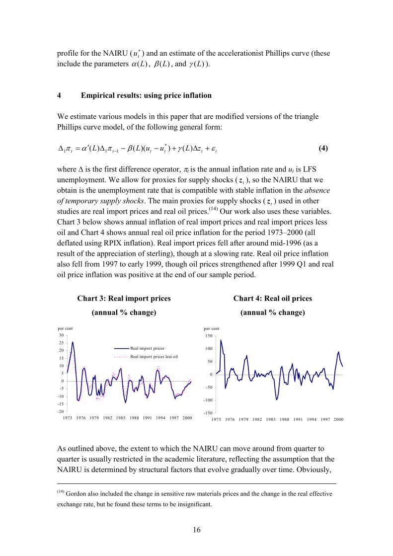
where � is the first difference operator, �t is the annual inflation rate and ut is LFSunemployment. We allow for proxies for supply shocks ( tz ), so the NAIRU that weobtain is the unemployment rate that is compatible with stable inflation in the absenceof temporary supply shocks. The main proxies for supply shocks ( tz ) used in otherstudies are real import prices and real oil prices.(14) Our work also uses these variables.Chart 3 below shows annual inflation of real import prices and real import prices lessoil and Chart 4 shows annual real oil price inflation for the period 1973–2000 (alldeflated using RPIX inflation). Real import prices fell after around mid-1996 (as aresult of the appreciation of sterling), though at a slowing rate. Real oil price inflationalso fell from 1997 to early 1999, though oil prices strengthened after 1999 Q1 and realoil price inflation was positive at the end of our sample period.
Chart 3: Real import prices
(annual % change)
Chart 4: Real oil prices
(annual % change)
-20
-15
-10
-5
0
5
10
15
20
25
30
1973 1976 1979 1982 1985 1988 1991 1994 1997 2000
Real import prices
Real import prices less oil
per cent
-150
-100
-50
0
50
100
150
1973 1976 1979 1982 1985 1988 1991 1994 1997 2000
per cent
As outlined above, the extent to which the NAIRU can move around from quarter toquarter is usually restricted in the academic literature, reflecting the assumption that theNAIRU is determined by structural factors that evolve gradually over time. Obviously,
(14) Gordon also included the change in sensitive raw materials prices and the change in the real effectiveexchange rate, but he found these terms to be insignificant.

17
the choice of this restriction (the signal-to-noise ratio) is to some degree arbitrary andthere is no universally accepted rule as to how to impose this restriction. We estimate arange of models using a general to specific estimation strategy based on a restriction forthe signal-to-noise ratio of 0.16 (one of the higher values used in Gordon (1997)). TheNAIRU profiles are influenced by this restriction and we do not suggest that this valueis necessarily the United Kingdom’s ‘true’ value. The sensitivity of the NAIRU profilesto other values for the signal-to-noise ratio is demonstrated in Section 7 below. All theestimates shown in this paper are smoothed NAIRU estimates (which use the fullinformation set) rather than filtered estimates (which only use the information availableat the time that the forecast was made).
Table A below shows the results of estimating models for RPIX inflation for the periodfrom 1973 to 2000. We employ a general to specific estimation testing (omittinginsignificant variables), where our regressors were the current value of theunemployment gap (the ‘demand’ effect in the triangle model), lagged annual RPIXinflation terms (capturing inertia) and lagged real import price inflation and real oilprice inflation terms (the ‘supply’ component). The first row of Table A shows thatchanges in inflation are negatively correlated with the unemployment gap, suggestingthat when unemployment is below the NAIRU, it will put upward pressure on inflationand inflation will tend to rise, though effects from the inertia and supply components inthe model may offset this pressure.(15)
In other empirical papers, it is common to include at least one additional lag of theunemployment gap (since if there is at least one lag, the effect from the change in thedemand variable on inflation is automatically captured (see Gordon (1997, page 16)).Gordon (1997, 1998) allows the unemployment rate to enter both contemporaneouslyand lagged, whereas Staiger, Stock and Watson (1997a) use specifications where onlylagged values of the unemployment gaps enter. We allowed for both possibilities in ourestimation strategy. When the lagged unemployment gap was added to our list ofregressors, then the contemporanous value of the unemployment gap becameinsignificant and so this latter term was excluded from our model (this resulted inmodel 2). And when the general model was based on only lagged values of theunemployment gap (ie similar to the Staiger, Stock and Watson (1997a)), only, thelagged unemployment gap in period 1 was strongly significant (again deliveringmodel 2). So, for our RPIX-based models, both estimation strategies deliver the same
(15) Preliminary work (based on an HP-filtered NAIRU) suggested that the equation diagnostics wereimproved by the inclusion of a dummy (=-1 in 1979 Q3, 1 in 1980 Q3, 0 at all other times). An oil priceshock and VAT change occurred around this time, and this result suggests that normally distributed errorscould only be achieved by including a dummy variable for this period.
18
model. Further, additional lags of the dependent variable were not statisticallysignificant at conventional levels of testing and so were excluded.(16)
The final row in the table reports the log-likelihood (LL) for each model. A likelihoodratio (LR) test suggests that deleting any of the ‘supply’ variables leads to an inferiormodel.(17)
Since oil prices feed through into import prices, total import prices may to some extentcontain the same information as the oil price term. To avoid the possibility ofdouble-counting, an alternative is to use a real import price series stripping out oiltogether with real oil price series as our supply shock variables (models 3 and 4 below).Using a general to specific estimation approach based on the current unemployment gapdelivers model 3. However, when lagged unemployment gaps were added to ourgeneral specification, once again, its lagged value in period 1 dominated either thecontemporanous term or the additional lagged terms, resulting in model 4.
There is also the question as to what is the appropriate price deflator that should bemodelled. Some papers (such as Gordon (1997)) use a variety of measures. In additionto RPIX, we employed a general to specific estimation strategy for models based on theconsumers’ expenditure deflator. The results were broadly similar to those reportedabove. There was a statistically significant relationship between the unemployment gapand changes in inflation and once again, the results were dominated by the inclusion ofthe gap term in the previous period. Changes in real import prices were significant,though this was not the case for real oil prices. The results are given in the final columnof Table A (Section 6 below compares the NAIRU profiles).(18)
To summarise the findings of Table A, the lagged unemployment gap appears to play animportant role in the inflation process. Our results suggest that it is more influentialthan either the contemporaneous value of the unemployment gap or further lags (sincewhen these terms are included, the lagged term in period 1 remains statisticallysignificant at the expense of other terms). But in terms of the overall specification, thereis little difference in the coefficients or the fit of these models. Excluding any of thesupply-side variables would lead to an inferior model. Thus, model 2 will be consideredas our ‘preferred’ RPIX-based model.
(16) For example, when ���t-2 was added to model 2, the t-statistic was –1.58. For other models considered,it was even less significant.(17) The likelihood ratio test is simply 2*(LL(unrestricted model)-LL(restricted model)) which isdistributed as �2(no of restrictions). In the case where there is one restriction, a difference in thelikelihoods reported in the tables of 1.92 or higher (=3.84/2) means that the restricted model can berejected at the 95% level of confidence.(18) Preliminary work (based on an HP-filtered NAIRU) suggested that the equation diagnostics wereimproved by the inclusion of the same dummy in 1979/1980, as well as a dummy for 1977 Q4.

19
Table A: Price inflation Phillips curve models estimated using the Kalman filter,1973 Q1–2000 Q4
Dependent variable��t (rpix)
RPIX(1)
RPIX(2)
RPIX(3)
RPIX(4)
Dependent variable��t (personal
consumption deflator)
PC(1)
*tt uu � -0.41
[-4.43]
- -0.55[-4.73]
- -
*11 ��
� tt uu - -0.43[-4.74]
- -0.57[-4.63]
-0.42[-5.10]
2�� t� - - - - -
4�� t� -0.32[-4.87]
-0.34[-5.18]
-0.31[-4.64]
-0.34[-4.95]
-0.34[-5.50]
�Real import price
Inflation t – 1
0.34[3.58]
0.37[3.88]
- - 0.34[4.34]
�Real import price
Inflation t - 4
0.25[2.34]
0.25[2.31]
- - 0.33[4.37]
�Real oil price
Inflation t - 3
- - - 0.27[3.03]
-
�Real oil price
Inflation t - 4
0.22[2.14]
0.19[1.84]
0.35[4.03]
- -
�Real import price
(Less oil) inflation t – 1
- - 0.39[3.75]
0.38[3.58]
-
D79/80 -3.79[-6.65]
-3.84[-6.78]
-4.10[-7.42]
-4.16[-7.56]
-3.17[-7.37]
D77Q4 - - - - -3.08[-4.92]
LL -139.5 -139.3 -141.4 -141.7 -112.7
LL is the log-likelihood, t-statistics are in parentheses.

20
Chart 5 shows the NAIRU profiles for models 1 and 2 in Table A above and Chart 6shows the profiles for models 3 and 4 for the period from 1973 to 2000. The generalshape of the profiles is similar, even though we are allowing the profiles to be quitevolatile. All models show the NAIRU peaking in the mid-1980s and tending to fallback thereafter. This is consistent with a range of NAIRU estimates produced using astructural approach (see Coulton and Cromb (1994)). The models tend to show thatactual unemployment was below the NAIRU in the second half of the 1990s, but theextent of this gap differs. The smoothness of the fall in the NAIRU in the 1990s alsovaries according to the model used. The models shown in Chart 5 are characterised by asteep decline in the estimated NAIRU during the second half of the 1980s and a slightrise in the early 1990s, declining again after around 1993.
Chart 5: Unemployment and u* profiles
from models 1, 2 and 3a (per cent)
Chart 6: Unemployment and u* profiles
from models 3 and 4 (per cent)
0
2
4
6
8
10
12
14
1973 1976 1979 1982 1985 1988 1991 1994 1997 2000
u u*(1) u*(2)
0
2
4
6
8
10
12
14
1973 1976 1979 1982 1985 1988 1991 1994 1997 2000
u u*(3) u*(4)
If no supply-shock variables (such as import prices) were included in the model, then inan arithmetic sense, given the RPIX outturn, the NAIRU profile without supply-sidevariables would be lower for much of the period since 1997 (as real import priceinflation has been negative during this period). The implication is that temporary supplyshocks, such as the appreciation of sterling (which has led to lower import prices), havehad a beneficial impact on RPIX inflation. In order to investigate this more fully, astatic contributions exercise was undertaken for model 2. The results (which areexpressed in terms of annual inflation) are shown in Chart 7 below.
Unsurprisingly, inertia, or lagged inflation, is a key influence on current RPIX inflation.Following an upturn in economic activity, unemployment tends to fall below the estimatedlevel of the NAIRU and this negative unemployment gap puts upward pressure oninflation. This can be seen for the expansion towards the end of the 1980s and for theperiod 1997-2000. Similarly, in the early 1990s, unemployment was above the NAIRU
21
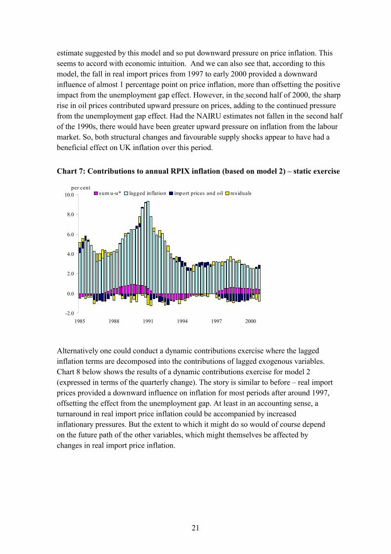
estimate suggested by this model and so put downward pressure on price inflation. Thisseems to accord with economic intuition. And we can also see that, according to thismodel, the fall in real import prices from 1997 to early 2000 provided a downwardinfluence of almost 1 percentage point on price inflation, more than offsetting the positiveimpact from the unemployment gap effect. However, in the second half of 2000, the sharprise in oil prices contributed upward pressure on prices, adding to the continued pressurefrom the unemployment gap effect. Had the NAIRU estimates not fallen in the second halfof the 1990s, there would have been greater upward pressure on inflation from the labourmarket. So, both structural changes and favourable supply shocks appear to have had abeneficial effect on UK inflation over this period.
Chart 7: Contributions to annual RPIX inflation (based on model 2) – static exercise
-2.0
0.0
2.0
4.0
6.0
8.0
10.0
1985 1988 1991 1994 1997 2000
sum u-u* lagged inflation import prices and oil res idualsper cent
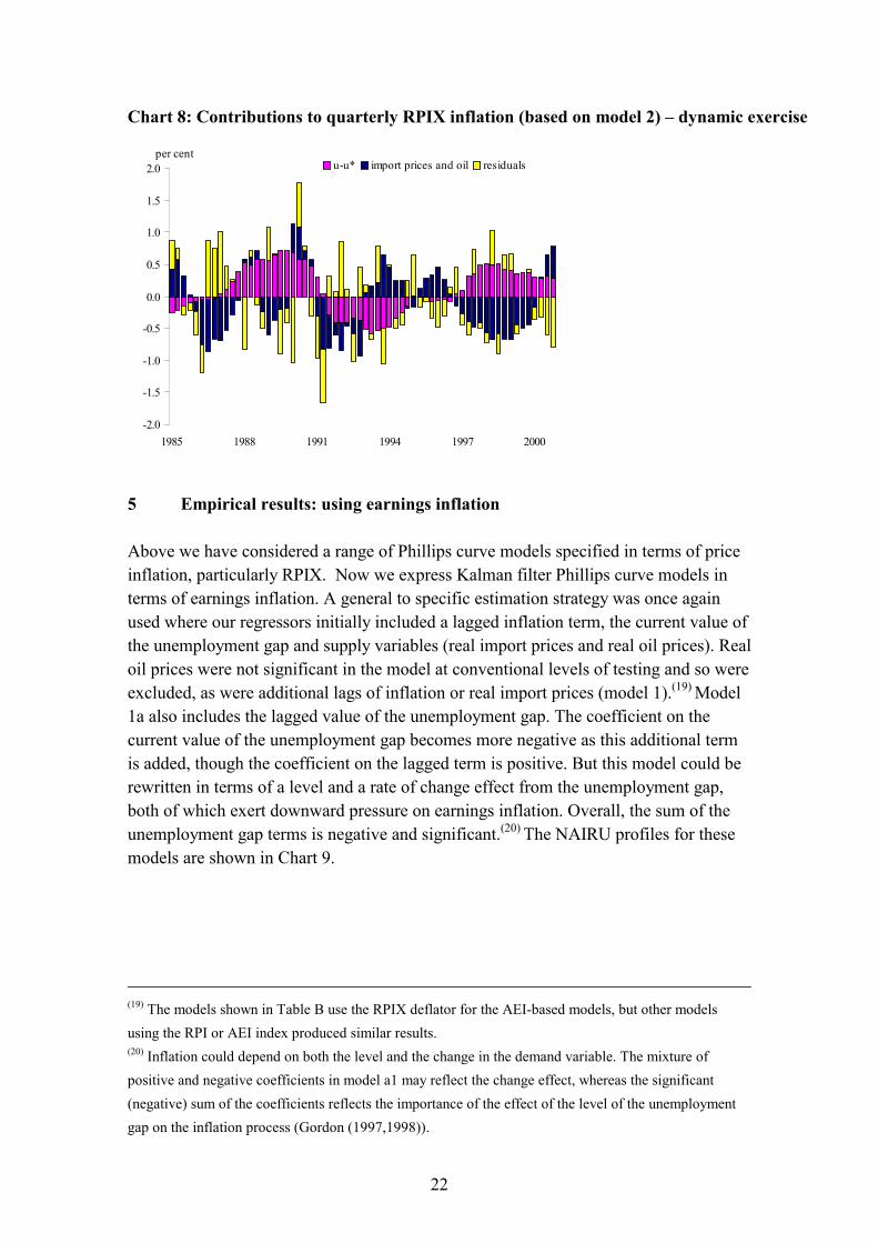
Alternatively one could conduct a dynamic contributions exercise where the laggedinflation terms are decomposed into the contributions of lagged exogenous variables.Chart 8 below shows the results of a dynamic contributions exercise for model 2(expressed in terms of the quarterly change). The story is similar to before – real importprices provided a downward influence on inflation for most periods after around 1997,offsetting the effect from the unemployment gap. At least in an accounting sense, aturnaround in real import price inflation could be accompanied by increasedinflationary pressures. But the extent to which it might do so would of course dependon the future path of the other variables, which might themselves be affected bychanges in real import price inflation.
22
Chart 8: Contributions to quarterly RPIX inflation (based on model 2) – dynamic exercise
-2.0
-1.5
-1.0
-0.5
0.0
0.5
1.0
1.5
2.0
1985 1988 1991 1994 1997 2000
u-u* import prices and oil residualsper cent
5 Empirical results: using earnings inflation
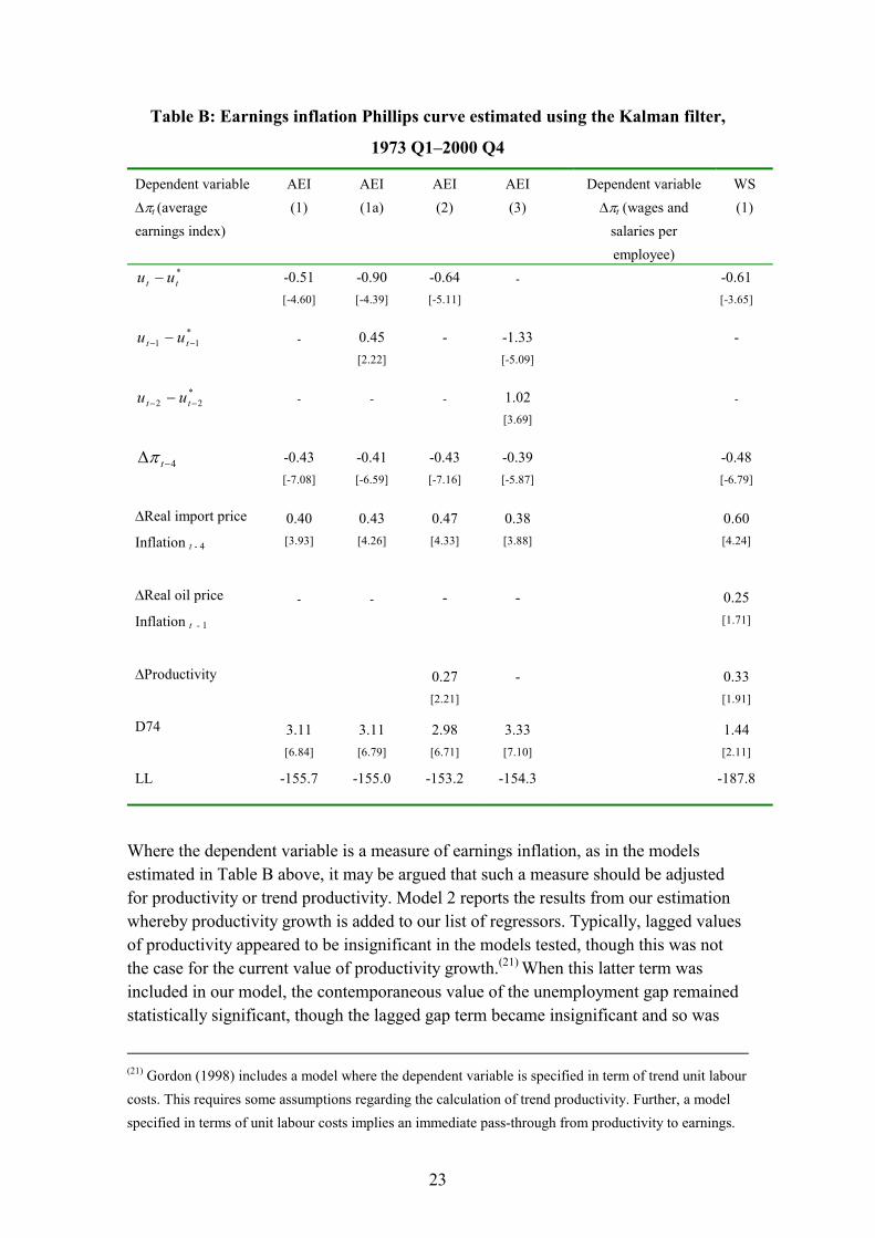
Above we have considered a range of Phillips curve models specified in terms of priceinflation, particularly RPIX. Now we express Kalman filter Phillips curve models interms of earnings inflation. A general to specific estimation strategy was once againused where our regressors initially included a lagged inflation term, the current value ofthe unemployment gap and supply variables (real import prices and real oil prices). Realoil prices were not significant in the model at conventional levels of testing and so wereexcluded, as were additional lags of inflation or real import prices (model 1).(19) Model1a also includes the lagged value of the unemployment gap. The coefficient on thecurrent value of the unemployment gap becomes more negative as this additional termis added, though the coefficient on the lagged term is positive. But this model could berewritten in terms of a level and a rate of change effect from the unemployment gap,both of which exert downward pressure on earnings inflation. Overall, the sum of theunemployment gap terms is negative and significant.(20) The NAIRU profiles for thesemodels are shown in Chart 9.
(19) The models shown in Table B use the RPIX deflator for the AEI-based models, but other modelsusing the RPI or AEI index produced similar results.(20) Inflation could depend on both the level and the change in the demand variable. The mixture ofpositive and negative coefficients in model a1 may reflect the change effect, whereas the significant(negative) sum of the coefficients reflects the importance of the effect of the level of the unemploymentgap on the inflation process (Gordon (1997,1998)).
23
Table B: Earnings inflation Phillips curve estimated using the Kalman filter,
1973 Q1–2000 Q4
Dependent variable��t (averageearnings index)
AEI(1)
AEI(1a)
AEI(2)
AEI(3)
Dependent variable��t (wages and
salaries peremployee)
WS(1)
*tt uu � -0.51
[-4.60]
-0.90[-4.39]
-0.64[-5.11]
- -0.61[-3.65]
*11 ��
� tt uu - 0.45[2.22]
- -1.33[-5.09]
-
*22 ��
� tt uu - - - 1.02[3.69]
-
4�� t� -0.43[-7.08]
-0.41[-6.59]
-0.43[-7.16]
-0.39[-5.87]
-0.48[-6.79]
�Real import price
Inflation t - 4
0.40[3.93]
0.43[4.26]
0.47[4.33]
0.38[3.88]
0.60[4.24]
�Real oil price
Inflation t - 1
- - - - 0.25[1.71]
�Productivity 0.27[2.21]
- 0.33[1.91]
D74 3.11[6.84]
3.11[6.79]
2.98[6.71]
3.33[7.10]
1.44[2.11]
LL -155.7 -155.0 -153.2 -154.3 -187.8
Where the dependent variable is a measure of earnings inflation, as in the modelsestimated in Table B above, it may be argued that such a measure should be adjustedfor productivity or trend productivity. Model 2 reports the results from our estimationwhereby productivity growth is added to our list of regressors. Typically, lagged valuesof productivity appeared to be insignificant in the models tested, though this was notthe case for the current value of productivity growth.(21) When this latter term wasincluded in our model, the contemporaneous value of the unemployment gap remainedstatistically significant, though the lagged gap term became insignificant and so was
(21) Gordon (1998) includes a model where the dependent variable is specified in term of trend unit labourcosts. This requires some assumptions regarding the calculation of trend productivity. Further, a modelspecified in terms of unit labour costs implies an immediate pass-through from productivity to earnings.
24
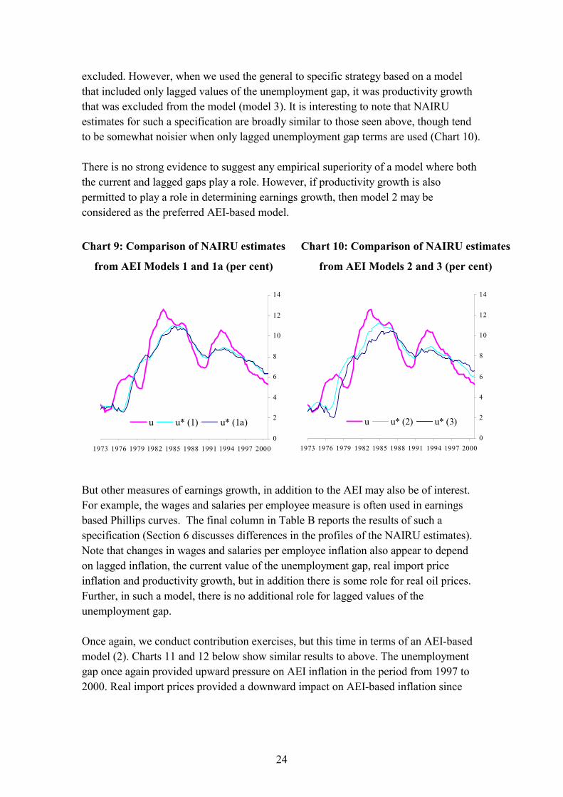
excluded. However, when we used the general to specific strategy based on a modelthat included only lagged values of the unemployment gap, it was productivity growththat was excluded from the model (model 3). It is interesting to note that NAIRUestimates for such a specification are broadly similar to those seen above, though tendto be somewhat noisier when only lagged unemployment gap terms are used (Chart 10).
There is no strong evidence to suggest any empirical superiority of a model where boththe current and lagged gaps play a role. However, if productivity growth is alsopermitted to play a role in determining earnings growth, then model 2 may beconsidered as the preferred AEI-based model.
Chart 9: Comparison of NAIRU estimates
from AEI Models 1 and 1a (per cent)
Chart 10: Comparison of NAIRU estimates
from AEI Models 2 and 3 (per cent)
0
2
4
6
8
10
12
14
1973 1976 1979 1982 1985 1988 1991 1994 1997 2000
u u* (1) u* (1a)0
2
4
6
8
10
12
14
1973 1976 1979 1982 1985 1988 1991 1994 1997 2000
u u* (2) u* (3)
But other measures of earnings growth, in addition to the AEI may also be of interest.For example, the wages and salaries per employee measure is often used in earningsbased Phillips curves. The final column in Table B reports the results of such aspecification (Section 6 discusses differences in the profiles of the NAIRU estimates).Note that changes in wages and salaries per employee inflation also appear to dependon lagged inflation, the current value of the unemployment gap, real import priceinflation and productivity growth, but in addition there is some role for real oil prices.Further, in such a model, there is no additional role for lagged values of theunemployment gap.
Once again, we conduct contribution exercises, but this time in terms of an AEI-basedmodel (2). Charts 11 and 12 below show similar results to above. The unemploymentgap once again provided upward pressure on AEI inflation in the period from 1997 to2000. Real import prices provided a downward impact on AEI-based inflation since

25
around mid-1997, though to a slightly lower degree than suggested by the RPIXmodel.(22) (23)
Chart 11: Contributions to AEI inflation (based on model 2) – static exercise
-4.0
-2.0
0.0
2.0
4.0
6.0
8.0
10.0
12.0
1985 1988 1991 1994 1997 2000
sum u-u* lagged inflation import prices productivity residuals
per cent
Chart 12: Contributions to AEI inflation (based on model 2) – dynamic exercise
-2.5
-2.0
-1.5
-1.0
-0.5
0.0
0.5
1.0
1.5
2.0
1985 1988 1991 1994 1997 2000
u-u* import prices productivity residualsper cent
(22) This effect on AEI inflation is likely to be indirect in practice, working through the pricing channel.(23) The large residual in 2000 Q2 is related to millenium effects. Annual wage inflation was boosted inearly 2000 by factors such as additional overtime. Annual wage inflation fell back noticeably in 2000 Q2.
26
6 Comparing NAIRU estimates from price and earnings models
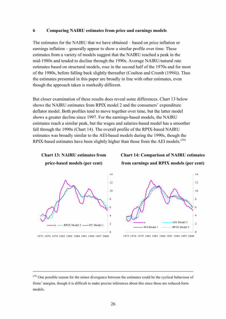
The estimates for the NAIRU that we have obtained – based on price inflation orearnings inflation – generally appear to show a similar profile over time. Theseestimates from a variety of models suggest that the NAIRU reached a peak in themid-1980s and tended to decline through the 1990s. Average NAIRU/natural rateestimates based on structural models, rose in the second half of the 1970s and for mostof the 1980s, before falling back slightly thereafter (Coulton and Cromb (1994)). Thusthe estimates presented in this paper are broadly in line with other estimates, eventhough the approach taken is markedly different.
But closer examination of these results does reveal some differences. Chart 13 belowshows the NAIRU estimates from RPIX model 2 and the consumers’ expendituredeflator model. Both profiles tend to move together over time, but the latter modelshows a greater decline since 1997. For the earnings-based models, the NAIRUestimates reach a similar peak, but the wages and salaries-based model has a smootherfall through the 1990s (Chart 14). The overall profile of the RPIX-based NAIRUestimates was broadly similar to the AEI-based models during the 1990s, though theRPIX-based estimates have been slightly higher than those from the AEI models.(24)
Chart 13: NAIRU estimates from
price-based models (per cent)
Chart 14: Comparison of NAIRU estimates
from earnings and RPIX models (per cent)
0
2
4
6
8
10
12
14
1973 1976 1979 1982 1985 1988 1991 1994 1997 2000
u RPIX Model 2 PC Model 1
0
2
4
6
8
10
12
14
1973 1976 1979 1982 1985 1988 1991 1994 1997 2000
u AEI Model 2
WS Model 1 RPIX Model 2
(24) One possible reason for the minor divergence between the estimates could be the cyclical behaviour offirms’ margins, though it is difficult to make precise inferences about this since these are reduced-formmodels.
27
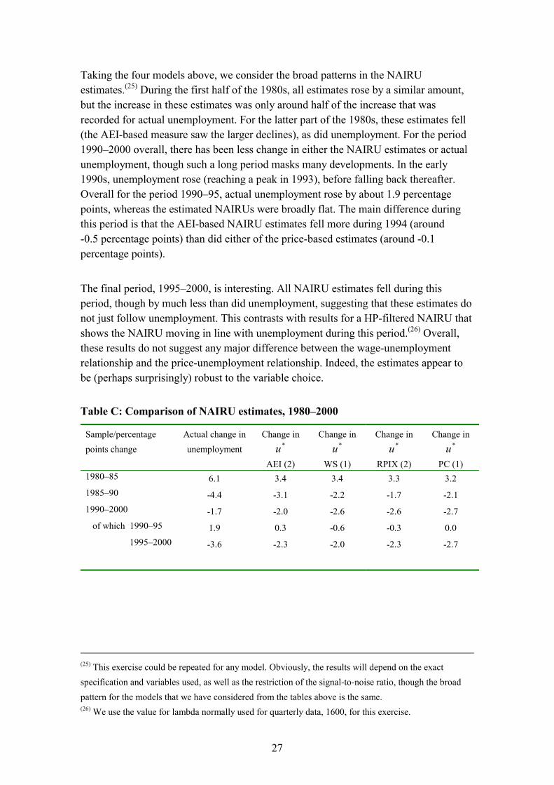
Taking the four models above, we consider the broad patterns in the NAIRUestimates.(25) During the first half of the 1980s, all estimates rose by a similar amount,but the increase in these estimates was only around half of the increase that wasrecorded for actual unemployment. For the latter part of the 1980s, these estimates fell(the AEI-based measure saw the larger declines), as did unemployment. For the period1990–2000 overall, there has been less change in either the NAIRU estimates or actualunemployment, though such a long period masks many developments. In the early1990s, unemployment rose (reaching a peak in 1993), before falling back thereafter.Overall for the period 1990–95, actual unemployment rose by about 1.9 percentagepoints, whereas the estimated NAIRUs were broadly flat. The main difference duringthis period is that the AEI-based NAIRU estimates fell more during 1994 (around-0.5 percentage points) than did either of the price-based estimates (around -0.1percentage points).
The final period, 1995–2000, is interesting. All NAIRU estimates fell during thisperiod, though by much less than did unemployment, suggesting that these estimates donot just follow unemployment. This contrasts with results for a HP-filtered NAIRU thatshows the NAIRU moving in line with unemployment during this period.(26) Overall,these results do not suggest any major difference between the wage-unemploymentrelationship and the price-unemployment relationship. Indeed, the estimates appear tobe (perhaps surprisingly) robust to the variable choice.
Table C: Comparison of NAIRU estimates, 1980–2000
Sample/percentagepoints change
Actual change inunemployment
Change in*u
AEI (2)
Change in*u
WS (1)
Change in*u
RPIX (2)
Change in*u
PC (1)1980–85 6.1 3.4 3.4 3.3 3.21985–90 -4.4 -3.1 -2.2 -1.7 -2.11990–2000 -1.7 -2.0 -2.6 -2.6 -2.7 of which 1990–95 1.9 0.3 -0.6 -0.3 0.0 1995–2000 -3.6 -2.3 -2.0 -2.3 -2.7
(25) This exercise could be repeated for any model. Obviously, the results will depend on the exactspecification and variables used, as well as the restriction of the signal-to-noise ratio, though the broadpattern for the models that we have considered from the tables above is the same.(26) We use the value for lambda normally used for quarterly data, 1600, for this exercise.
28
7 Sensitivity analysis
The NAIRU estimates above were all determined on the basis of a restriction of thesignal-to-noise ratio, consistent with the idea that the NAIRU should not jump aroundfrom quarter to quarter, but instead evolves more gradually over time. Below we showthe effect of using a wide range of restrictions for the ratio of the variances of the errorterms before providing some standard error bands. For conciseness, we conduct theseexercises using only an AEI-based model 1a above.
7.1 Restricting the signal-to-noise ratio
Though the variability of the NAIRU can in principle be estimated from the data, arestriction is usually adopted in the literature (this involves restricting the ratio of thevariances of the error terms ( 2
�� and 2
�� above)). For a given variation in ��, the signal-
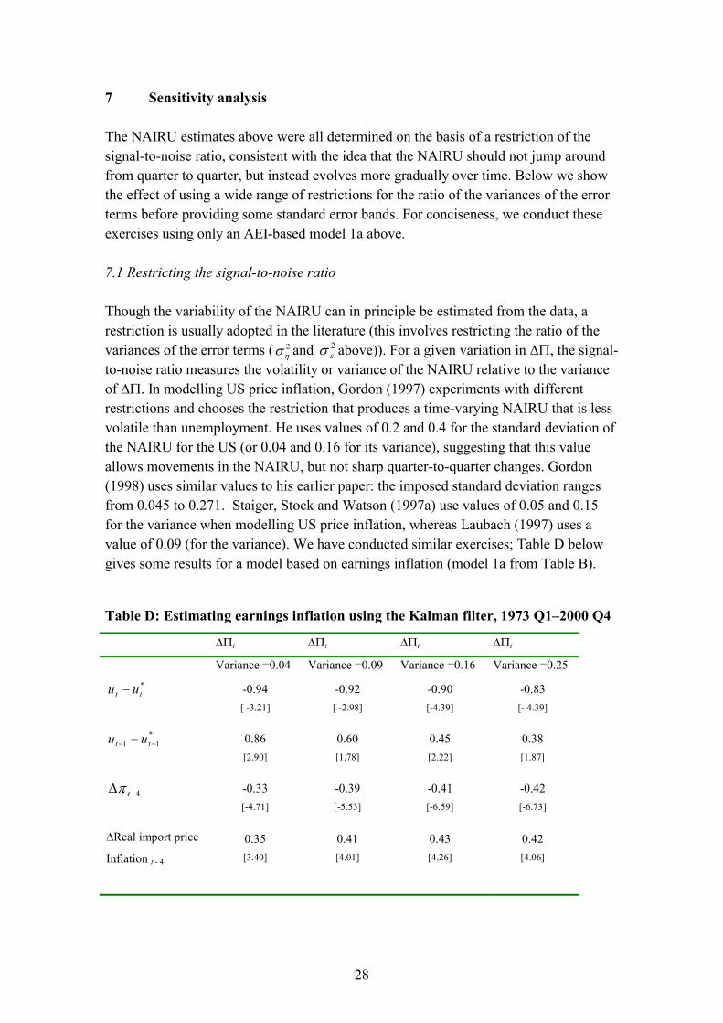
to-noise ratio measures the volatility or variance of the NAIRU relative to the varianceof ��. In modelling US price inflation, Gordon (1997) experiments with differentrestrictions and chooses the restriction that produces a time-varying NAIRU that is lessvolatile than unemployment. He uses values of 0.2 and 0.4 for the standard deviation ofthe NAIRU for the US (or 0.04 and 0.16 for its variance), suggesting that this valueallows movements in the NAIRU, but not sharp quarter-to-quarter changes. Gordon(1998) uses similar values to his earlier paper: the imposed standard deviation rangesfrom 0.045 to 0.271. Staiger, Stock and Watson (1997a) use values of 0.05 and 0.15for the variance when modelling US price inflation, whereas Laubach (1997) uses avalue of 0.09 (for the variance). We have conducted similar exercises; Table D belowgives some results for a model based on earnings inflation (model 1a from Table B).
Table D: Estimating earnings inflation using the Kalman filter, 1973 Q1–2000 Q4
��t ��t ��t ��t
Variance =0.04 Variance =0.09 Variance =0.16 Variance =0.25*tt uu � -0.94
[ -3.21]
-0.92[ -2.98]
-0.90[-4.39]
-0.83[- 4.39]
*11 ��
� tt uu 0.86[2.90]
0.60[1.78]
0.45[2.22]
0.38[1.87]
4�� t� -0.33[-4.71]
-0.39[-5.53]
-0.41[-6.59]
-0.42[-6.73]
�Real import price
Inflation t - 4
0.35[3.40]
0.41[4.01]
0.43[4.26]
0.42[4.06]
29
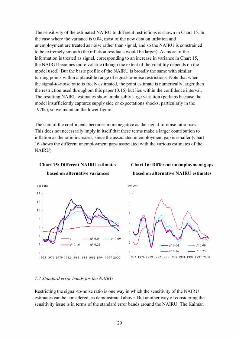
The sensitivity of the estimated NAIRU to different restrictions is shown in Chart 15. Inthe case where the variance is 0.04, most of the new data on inflation andunemployment are treated as noise rather than signal, and so the NAIRU is constrainedto be extremely smooth (the inflation residuals would be larger). As more of theinformation is treated as signal, corresponding to an increase in variance in Chart 15,the NAIRU becomes more volatile (though the extent of the volatility depends on themodel used). But the basic profile of the NAIRU is broadly the same with similarturning points within a plausible range of signal-to-noise restrictions. Note that whenthe signal-to-noise ratio is freely estimated, the point estimate is numerically larger thanthe restriction used throughout this paper (0.16) but lies within the confidence interval.The resulting NAIRU estimates show implausibly large variation (perhaps because themodel insufficiently captures supply side or expectations shocks, particularly in the1970s), so we maintain the lower figure.
The sum of the coefficients becomes more negative as the signal-to-noise ratio rises.This does not necessarily imply in itself that these terms make a larger contribution toinflation as the ratio increases, since the associated unemployment gap is smaller (Chart16 shows the different unemployment gaps associated with the various estimates of theNAIRU).
Chart 15: Different NAIRU estimates
based on alternative variances
Chart 16: Different unemployment gaps
based on alternative NAIRU estimates
0
2
4
6
8
10
12
14
1973 1976 1979 1982 1985 1988 1991 1994 1997 2000
per cent
u u* 0.04 u* 0.09
u* 0.16 u* 0.25
-4
-2
0
2
4
6
8
1973 1976 1979 1982 1985 1988 1991 1994 1997 2000
per cent
u* 0.04 u* 0.09
u* 0.16 u* 0.25
7.2 Standard error bands for the NAIRU
Restricting the signal-to-noise ratio is one way in which the sensitivity of the NAIRUestimates can be considered, as demonstrated above. But another way of considering thesensitivity issue is in terms of the standard error bands around the NAIRU. The Kalman

30
filter approach allows us to do this, as do some other approaches. For an excellentexample of different techniques to derive estimates of the US NAIRU, see Staiger,Stock and Watson (1997a). Using various methods, they found that the confidenceintervals around the US NAIRU were large.(27)
We calculate confidence intervals for the NAIRU using AEI-based model 1a above.(28)
We consider only the filter uncertainty that is calculated from the smoothing iteration.This represents uncertainty that would be present even if true values of the parameterswere known.(29) Chart 17 below shows an example of the standard error bands,confirming that both the 90% and 95% confidence intervals around the NAIRU arewide. This is in line with the findings of Cross, Darby and Ireland (1997) who used avariety of specifications, but not the Kalman filter approach, to derive estimates of theconfidence intervals for the NAIRU and found a large degree of uncertainty aroundthese estimates. Using their preferred specification for the UK (which allowed a meanshift in unemployment), the 95% confidence intervals for the NAIRU were in the rangeof 7.41 to 10.29 for the period 1980 Q1–1995 Q3. However, for an alternativeapproach, based on a 2 knot cubic spline specification, the 95% confidence intervalswere between –9.98 and 14.55 for 1994 Q1. Our findings confirm the general belief thatestimates of the NAIRU tend to be imprecisely measured, suggesting that suchestimates should be treated with caution. For example, at times, we may be 90% certainthat actual unemployment has not been above (or below) the NAIRU. However, thisinformation may still be useful, though it does suggest not placing too much emphasison a particular point estimate.
(27) For their Kalman filter based time-varying models, the standard errors reported for the NAIRU are thesquare root of the sum of the Kalman smoothed estimates of the variance of the state and the delta methodestimate of the variance of the estimate of the state (Ansley and Kohn (1986)).(28) We use a signal-to-noise restriction of 0.16. The confidence intervals will depend on the amount ofvariation allowed in the NAIRU to some extent. Laubach (1997) notes a positive correlation between thewidth of the confidence intervals and the volatility in the NAIRU. We find the opposite – as the NAIRUis allowed to move more, the estimated standard errors are smaller. This matches the result in Boone(2000).(29) One could in principle also calculate the parameter uncertainty by Monte Carlo simulations. We leavethis as a possible future extension.
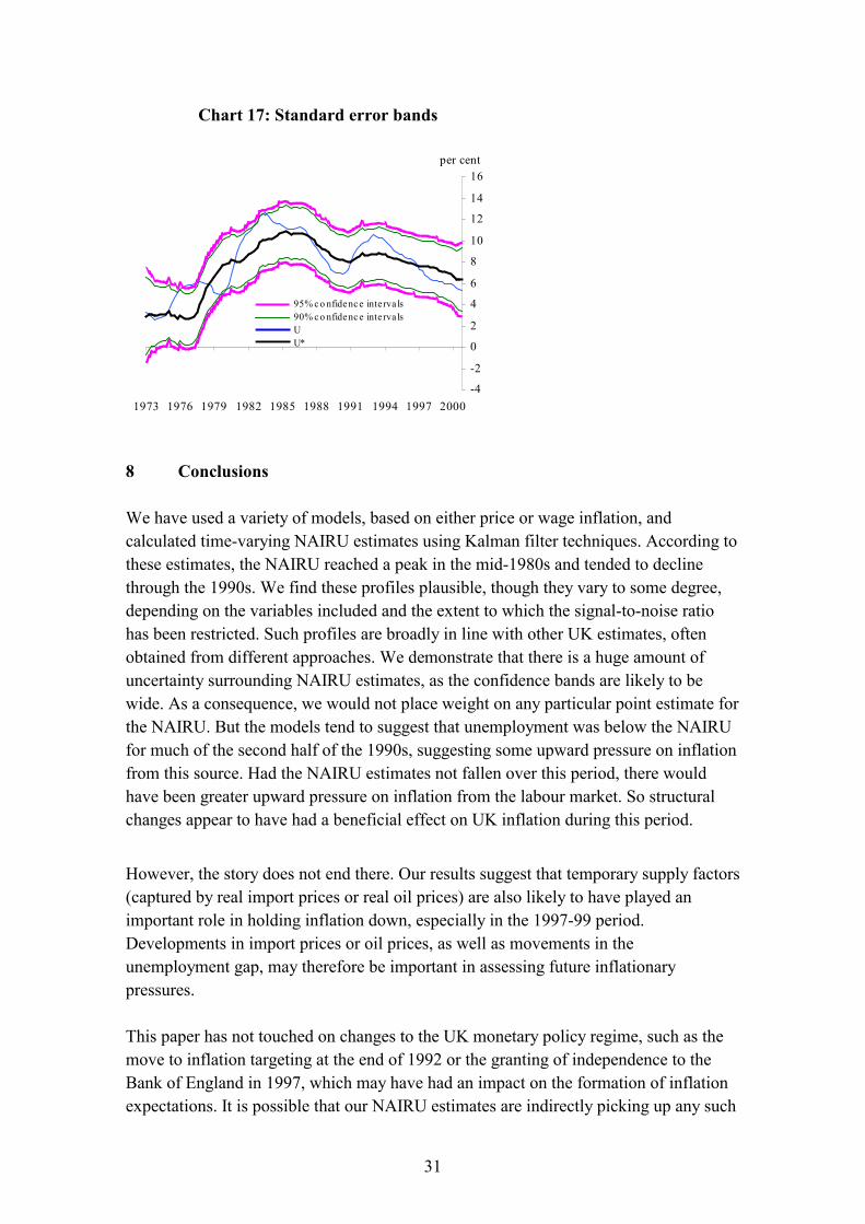
31
Chart 17: Standard error bands
-4
-2
0
2
4
6
8
10
12
14
16
1973 1976 1979 1982 1985 1988 1991 1994 1997 2000
per cent
95% c o nfidenc e interva ls90% c o nfidenc e interva lsUU*
8 Conclusions
We have used a variety of models, based on either price or wage inflation, andcalculated time-varying NAIRU estimates using Kalman filter techniques. According tothese estimates, the NAIRU reached a peak in the mid-1980s and tended to declinethrough the 1990s. We find these profiles plausible, though they vary to some degree,depending on the variables included and the extent to which the signal-to-noise ratiohas been restricted. Such profiles are broadly in line with other UK estimates, oftenobtained from different approaches. We demonstrate that there is a huge amount ofuncertainty surrounding NAIRU estimates, as the confidence bands are likely to bewide. As a consequence, we would not place weight on any particular point estimate forthe NAIRU. But the models tend to suggest that unemployment was below the NAIRUfor much of the second half of the 1990s, suggesting some upward pressure on inflationfrom this source. Had the NAIRU estimates not fallen over this period, there wouldhave been greater upward pressure on inflation from the labour market. So structuralchanges appear to have had a beneficial effect on UK inflation during this period.
However, the story does not end there. Our results suggest that temporary supply factors(captured by real import prices or real oil prices) are also likely to have played animportant role in holding inflation down, especially in the 1997-99 period.Developments in import prices or oil prices, as well as movements in theunemployment gap, may therefore be important in assessing future inflationarypressures.
This paper has not touched on changes to the UK monetary policy regime, such as themove to inflation targeting at the end of 1992 or the granting of independence to theBank of England in 1997, which may have had an impact on the formation of inflationexpectations. It is possible that our NAIRU estimates are indirectly picking up any such

32
changes, thus casting doubt on our estimates. But separate work including inflationexpectations does not provide any strong evidence that this was a key factor for theUnited Kingdom (see Driver, Greenslade and Pierse (2003)).

33
Appendix A: Data definitions
We use ONS data where available (ONS codes in parentheses).
Prices: Retail Price Index excluding mortgage interest payments (RPIX) since 1974[code CHMK]. Prior to 1974, we obtain a series for RPIX by applying the growth rateson the changes in the RPI index [code CHAW] to the level of RPIX in 1974.
Prices: Total Final Consumers’ Expenditure deflator (PC) [code (ABJK+HAYE) /(ABJR+HAYO)].
Earnings: Average Earnings Index (AEI) [code LNMQ].
Earnings: Wages and Salaries per employee (WS). This is wages and salaries from thenational accounts [code DTWL] divided by the sum of employees in employment plusHM Forces.
Unemployment: LFS unemployment from 1984 [code MGSX] and OECD measureprior to 1984.
Real import prices: Nominal total import prices are given by the implicit import pricedeflator [code = IKBI/IKBL] and import prices less oil are total trade in goods less oil[code BQKL]. In both cases import prices are deflated using RPIX or relevant pricedeflator.
Real oil prices: Brent oil prices in US dollars [code IFS.UK.IFS.11276AAZZF]converted into pounds sterling [code AJFA]. This series is also deflated using RPIX orrelevant price deflator.
Productivity: Output per head [code LNNN].
34
Appendix B: Kalman filter technique
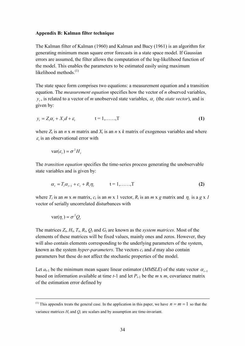
The Kalman filter of Kalman (1960) and Kalman and Bucy (1961) is an algorithm forgenerating minimum mean square error forecasts in a state space model. If Gaussianerrors are assumed, the filter allows the computation of the log-likelihood function ofthe model. This enables the parameters to be estimated easily using maximumlikelihood methods.(1)
The state space form comprises two equations: a measurement equation and a transitionequation. The measurement equation specifies how the vector of n observed variables,
ty , is related to a vector of m unobserved state variables, t� (the state vector), and isgiven by:
ttttt dXZy �� ��� t = 1,……,T (1)
where Zt is an n x m matrix and Xt is an n x k matrix of exogenous variables and wheret� is an observational error with
tt H2)var( �� �
The transition equation specifies the time-series process generating the unobservablestate variables and is given by:
tttttt RcT ��� ����1 t = 1,……,T (2)
where Tt is an m x m matrix, ct is an m x 1 vector, Rt is an m x g matrix and t� is a g x 1vector of serially uncorrelated disturbances with
tt Q2)var( �� �
The matrices Zt, Ht, Tt, Rt, Qt and Gt are known as the system matrices. Most of theelements of these matrices will be fixed values, mainly ones and zeros. However, theywill also contain elements corresponding to the underlying parameters of the system,known as the system hyper-parameters. The vectors ct and d may also containparameters but these do not affect the stochastic properties of the model.
Let at-1 be the minimum mean square linear estimator (MMSLE) of the state vector 1�t�
based on information available at time t-1 and let Pt-1 be the m x m, covariance matrixof the estimation error defined by
(1) This appendix treats the general case. In the application in this paper, we have 1�� mn so that the
variance matrices Ht and Qt are scalars and by assumption are time-invariant.

35
))(( 11111 ��������� ttttt aaEP ��
Then the Kalman filter comprises two sets of recursive equations: the predictionequations and the updating equations.
The prediction equations give the optimal predictors of the state vector t� and itscovariance matrix based on information available at time t-1.
ttttt caTa ���� 11| (3)
���� tttttttt RQRTPTP 11| (4)
The updating equations update this predictor using new information available at time tembodied in the prediction error
dXaZyv tttttt ����1| (5)
The updating equations are given by:
tttttttt vFZPaa 11| 1|
�
��
�� (6)
and
1| 1
1| 1| �
�
��
�� tttttttttt PZFZPPP (7)
where
tttttt HZPZF ���1|
Thus, the Kalman Filter is a recursive process for calculating the optimal estimator ofthe state vector given the information set at that time. The repeated process of optimalprediction, getting the prediction errors and updating the predictions are the essence ofthe Kalman filter algorithm.
Assuming that the disturbances are normally distributed, the log-likelihood function forthe model can be computed from the prediction errors vt and their associated covariancematrix Ft and is defined by:
t
T
ttt
T
tt vFvFnTL ��
�
�
�
�����
1
12
1
2
21log
21)2log(
2 �
�� (8)

36
The Kalman filter predictors 1| �tta and 1| �ttP give the optimal predictors of the statevector t� and its covariance matrix based on information available at time t-1. So thisprocedure of obtaining filtered estimates of unobserved state variable (in this case theNAIRU) does not use all the available information. The Kalman filter allows abackward recursion known as smoothing. The smoothed estimators Tta | and TtP | give theoptimal predictors of t� and )var( t� based on all the information in the sample. Thesesmoothed estimators can be generated from the backward recursions
)( 1|1*
| tttTtttTt caTaPaa ������
(9)
and
�����
*|1|1
*| )( tttTtttTt PPPPPP (10)
where
1|11
* �
��� ttttt PTPP
If ttP |1� is singular, its inverse can be replaced by a generalised inverse �
� ttP |1 .
37
References
Adams, C and Coe, D T (1990), ‘A systems approach to estimating the natural rate ofunemployment and potential output for the United States’, IMF Staff Papers, Vol. 37,pages 232–93.
Ansley, C and Kohn, R (1986), ‘Prediction mean squared error for state space modelswith estimated parameters’, Biometrika, Vol. 73(2), pages 467–73.
Apel, M and Jansson, P (1999), ‘System estimates of potential output and the NAIRU’,Empirical Economics, Vol. 24(3), August, pages 373–88.
Astley, M and Yates, A (1999), ‘Inflation and real disequilibria’, Bank of EnglandWorking Paper no. 103.
Bank of England (1999), Economic models at the Bank of England, Bank of England.
Barrell, R, Pain, N and Young, G (1994), ‘Structural differences in European labourmarkets’, in The UK labour market: comparative aspects and institutionaldevelopments, Cambridge University Press.
Barrell, R and Sefton, J (1995), ‘Output gaps. Some evidence from the UK, France andGermany’, National Institute Economic Review, No. 151, February, pages 65–73.
Barwell, R (2000), ‘Age structure and the UK unemployment rate’, Bank of EnglandWorking Paper no. 124.
Boone, L (2000), ‘Comparing semi-structural methods to estimate unobserved variables:the HPMV and Kalman filter approaches’, OECD Economic Department Working Paperno. 240.
Cassino, V and Thornton, R (2002), ‘Reduced-form estimates of the natural rate ofunemployment based on structural variables’, Bank of England Working Paper no. 153.
Cerra, V and Saxena, S C (2000), ‘Alternative methods of estimating potential outputand the output gap – an application to Sweden’, IMF Working Paper WP/00/59.
Coulton, B and Cromb, R (1994), ‘The UK NAIRU’, Government Economic ServiceWorking Paper no. 124.
Cromb, R (1993), ‘A survey of recent econometric work on the NAIRU’, Journal ofEconomic Studies, Vol. 20, pages 27–51.
38
Cross, R, Darby, J and Ireland, J (1997), ‘Uncertainties surrounding natural rateestimates in the G7’, Glasgow University Department of Economics Discussion Paper9712.
Debelle, G and Laxton, D (1997), ‘Is the Phillips curve really a curve? Some evidence forCanada, the United Kingdom, and the United States’, IMF Staff Papers, Vol. 44, pages249–82.
Driver, R, Greenslade, J V and Pierse, R G (2003), ‘The role of expectations inestimates of the NAIRU in the United States and the United Kingdom’, Bank of EnglandWorking Paper no. 180.
Friedman, M (1968), ‘The role of monetary policy’, American Economic Review, Vol. 58,pages 1–17.
Galí, J and Gertler, M (1999), ‘Inflation economics: a structural economic analysis’,Journal of Monetary Economics, Vol. 44(2), pages 195–222.
Giorno, C, Richardson, P, Roseveare, D and van de Noord, P (1995), ‘Potential output,output gaps and structural budget balances’, OECD Economic Studies, No. 24,pages 167–209.
Gordon, R J (1997), ‘The time-varying NAIRU and its implications for economic policy’,Journal of Economic Perspectives, Vol. 11(1), pages 11–32.
Gordon, R J (1998), ‘Foundations of the Goldilocks economy: supply shocks and thetime-varying NAIRU’, Brookings Papers on Economic Activity, Vol. II, pages 297–346.
Gruen, D, Pagan, A and Thompson, C (1999), ‘The Phillips curve in Australia’, Journalof Monetary Economics, Vol. 44, pages 223–58.
Hamilton, J (1994), Time series analysis, Princeton University Press.
Harvey, A C (1989), Forecasting, structural time series models and the Kalman filter,Cambridge University Press.
Harvey, A C (1993), Time series models, Harvester Wheatsheaf.
Hodrick, R J and Prescott, E C (1997), ‘Postwar U.S. business cycles: an empiricalinvestigation’, Journal of Money, Credit and Banking, Vol. 29, pages 1–16.
39
Kalman, R E (1960), ‘A new approach to linear filtering and prediction theory’, Journal ofBasic Engineering, Transactions ASME, Series D, Vol. 83, pages 35–45.
Kalman, R E and Bucy, R S (1961), ‘New results in linear filtering and predictiontheory’, Journal of Basic Engineering, Transactions ASME, Series D, Vol. 83,pages 95–108.
Katz, L M and Krueger, A B (1999), ‘The high-pressure U.S. labor market of the 1990s’,Brookings Papers on Economic Activity, Vol. (1), pages 1–65.
King, M (1999), ‘Monetary policy and the labour market’, Bank of England QuarterlyBulletin, Vol. 39, No. 1, pages 90–97.
Kuttner, K (1994), ‘Estimating potential output as a latent variable’, Journal of Businessand Economic Statistics, Vol. 12(3), pages 361–67.
Laubach, T (1997), ‘Measuring the NAIRU: evidence from seven economies’, FederalReserve Bank of Kansas City Working Paper no. 97–13.
Manning, A (1993), ‘Wage bargaining and the Phillips curve: the identification andspecification of aggregate wage equations’, Economic Journal, Vol. 103, pages 98–118.
Phelps, E S (1968), ‘Money-wage dynamics and labour market equilibrium’, Journalof Political Economy, Vol. 76, pages 678–711.
Phillips, AW (1958), ‘The relation between unemployment and the rate of change inmoney wages in the United Kingdom, 1861-1957’, Economica, Vol. 25, pages 283–99.
Rasi, C M and Viikari, J M (1998), ‘The time-varying NAIRU and potential output inFinland’, Bank of Finland Discussion Paper no. 6/98.
Roberts, J M (1995), ‘New Keynesian economics and the Phillips curve’, Journal ofMoney, Credit and Banking, Vol. 27, pages 974–84.
Roberts, J M (1997), ‘Is inflation sticky?’, Journal of Monetary Economics, Vol. 39,pages 173–96.
Staiger, D, Stock, J H and Watson, M W (1997a), ‘How precise are estimates of thenatural rate of unemployment?’, in Romer, C D and Romer, D H (eds), Reducing inflation:motivation and strategy, (NBER Research Studies in Business Cycles, Vol. 30, Universityof Chicago Press).

40
Staiger, D, Stock, J H and Watson, M W (1997b), ‘The NAIRU, unemployment andmonetary policy’, Journal of Economic Perspectives, Vol. 11(1), pages 33–49.
Turner, D, Boone, L, Giorno, C, Meacci, M, Rae, D and Richardson, P (2001),‘Estimating the structural rate of unemployment for the OECD countries’, OECDEconomic Studies, No. 33, pages 171–216.