a hydrological study of the kipkaren...

1 | P a g e

UNIVERSITY OF NAIROBI

A HYDROLOGICAL STUDY OF THE KIPKAREN

CATCHMENT

By

Ochieng Collins,

F16/24071/2008

A project submitted as a partial fulfillment for the requirement for the award of the degree of

BACHELOR OF SCIENCE IN CIVIL ENGINEERING

MARCH 2014

You created this PDF from an application that is not licensed to print to novaPDF printer (http://www.novapdf.com)

http://www.novapdf.com

2 | P a g e

Abstract

The Kipkaren catchment is located in Nandi District of Rift Valley Province. The catchment

covers three administrative locations namely; Kipkaren, Ndalat and Ngenyilel locations .The

Kipkaren River Basin is part of Lake Victoria North Catchment Area (LVN) which is part of

the Lake Victoria basin in Kenya. The catchment has an area of about 3234.4km2.The main

township in the area is Eldoret town.

Kipkaren catchment was chosen as the study catchment in order to study the rainfall and

streamflow data. The study sets four objectives, the first is to derive the seasonal rainfall

pattern of the catchment; the second is to determine the average rainfall of the catchment; the

third is to estimate the Storage required for the catchment, and the fourth objective is to

determine the flow duration and the low flow of the catchment.

In this study, the project assess the storage and flow durations in the catchment for the water

resource development in the area. Kipkaren river would be useful for direct water supply. The

information can also be used in flood control, energy generation and industrial use since there

are industries in the Eldoret Region. Generally, land degradation in the upper parts of the

catchment has caused frequent flooding in the lower catchment, as reduced forest cover and

an increase in agricultural lands have generally been known to generate high surface runoff.

Analysis has also shown that the catchment has two rainy seasons: the short rain season from

August to October and the long rain season from– March to May. From low flow analysis it

was found out that for 5% low flow will be 9.5 cumecs meaning that for 5% low flow < 9.5

cumecs, 95% of the time the flow will be > 9.5 cumecs. Also from flow duration analysis it

was gotten that for 5% low flow of 0.064cumecs, 5% of the time flow < 0.064cumecs and

95% of the time flow > 0.064 cumecs.



3 | P a g e

Dedication

To almighty God for the life and strength He has granted me. To my late father who had

always believed in me even when I did not. To my mother, thank you for all the sacrifice you

made to give me the gift of education. To my sister, thank you for the love and emotional

support.



4 | P a g e

Acknowledgements

I would like to take this opportunity, with deepest gratitude, to thank my supervisor Mr. Sadrudin H. Charania for rigorously guiding me through the research process, advising and counseling me through this entire period of the project. He has sacrificed most of his precious time to help me with my project and taught me a lot of new things in hydrology. Without his guidance, it would have been very difficult for me to prepare a credible report. I shall be forever grateful.

To all the lecturers in the department of engineering, I would like to thank you for all the knowledge that you have passed not only to me but all the students at the civil engineering department. I would also like extend my gratitude to the staff at the Ministry of Environment, Water and Natural Resources, including Mr. Simintei Ole Kooke and Dr.Nyaoro for providing me with all the relevant data that I needed. I shall never forget your gratitude. I would like to thank all my classmates for all their support, constructive criticism and ideas, and also for their friendship and assistance. I would also like to express my sincere thanks to all my friends who have patiently extended all kind of help for accomplishing this undertaking. Most importantly I would like to thank my family for being there for me through it all. I thank them for all the financial and moral support they gave me. To them I am forever grateful.



5 | P a g e

TABLE OF CONTENTS ABSTRACT..................................................................................................... i

DEDICATION.................................................................................................. ii

ACKNOWLEDGEMENT................................................................................ iii

TABLE OF CONTENTS..................................................................................vi

LIST OF TABLES ........................................................................................... vii

LIST OF FIGURES ........................................................................................ viii

CHAPTER ONE............................................................................................. 1

1.0. INTRODUCTION..................................................................................... 1

1.1. Basin Characterisation............................................................................... 1

1.2: River Gauging Station ............................................................................... 3

1.2.1: Rainfall Station.........................................................................................5

1.2.2: Meteorological Station............................................................................. 6

1.3: Objective .................................................................................................. 7

1.3: Main Objective ......................................................................................... 7

1.3: Specific Objective .................................................................................... 7

1.4: Scope of Study............................................................................................ 7

CHAPTER TWO ............................................................................................. 8

2.0: LITERATURE

REVIEW............................................................................................................. 8

2.1: Introduction.................................................................................................. 8

2.2: Rainfall......................................................................................................... 8

2.2.1: Rainfall Seasonality in Nzoia ....................................................................9

2.2.2: Rainfall Abstraction................................................................................. 10

2.3: Runoff........................................................................................................ 11

2.3.1: Runoff Cycle.............................................................................................13

2.3.2: Factors Affecting Runoff …….................................................................16



6 | P a g e

CHAPTER THREE........................................................................................... 17

3.0: METHODOLOGY........................................................................................17

3.1: Research Approach ........................................................................................17

3.1.1: Data Processing…………………………………………..……………… 17

3.1.2: Rainfall Analysis........................................................................................ 18

3.1.2.1: Determination of Seasonal pattern......................................................... 18

3.1.2.2: Determination of Average Rainfall.........................................................18

3.1.2.3: Theissen Polygon Method………. ........................................................ 19

3.1.2.4: Probability Analysis of Precipitation ……………………….…………20

3.2: Stream flow Analysis .................................................................................. 20

3.2.1: Flow duration Analysis………………………………………………….21

3.2.2: Low Flow Analysis…………………………………………….………..22

3.2.3: Storage Analysis………………………………………………………….22

3.3: Data Collection……………………………………………………………..22

3.2.1: Rainfall and Streamflow data ................................................................... 23

CHAPTER FOUR...................................................................................... …..25

4.0: ANALYSIS AND DISCUSSION................................................................. 30

4.1: Rainfall Analysis & Discussion.......................................................................30

4.2: Stream Flow Analysis...................................................................................... 30

4.2.1: Flow Duration Analysis and Discussion........................................................ 32

4.2.2: Low Flow Analysis and Discussion. ..............................................................34

4.2.3: Storage analysis and Discussion .....................................................................36

CHAPTER FIVE ................................................................................................... 37

5.0: CONCLUSIONS AND RECOMMENDATIONS .......................................... 37

5.1: Conclusions ...................................................................................................... 37

5.2: Recommendations............................................................................................. 38

REFERENCES......................................................................................................... 40

APPENDIX.............................................................................................................. 41



7 | P a g e

Appendix A: Tables .................................................................................................41 Appendix B: Maps................................................................................................... 56

LIST OF TABLES

Table 1: Table of the Network of Stream Gauging Stations of Kipkaren Basin……………..3

Table 2: Table of Rainfall Stations Network of the Kipkaren Catchment…………………...5

Table 3: List of meteorological stations………………………………………………….…...6

Table 4: Table showing the filling in of missing data……………………………………..…17

Table 5: Tabulation format of the results…………………………………………….......…19

Table 6: Rainfall and stream flow stations used in this study………………………………23

Table 7: Mean monthly and mean annual rainfall of Station 8935181………………......…24

Table 8: Mean Annual Rainfall of station I.D.8935181-Eldoret Meteorological Station…..26

Table 9: Statistical Analysis of the Precipitation of Station no. 8935181………………….26

Table 10: Mean monthly and mean annual rainfall of Station no.8935076 ………………..27

Table 11: Mean Annual Rainfall of Station No.8935076…………………………………..29

Table 12: Theissen Polygon method of finding average rainfall……………………….…..30

Table 13: Monthly Summary of the Flow of Gauging Station 1CE01………………….….31

Table 14: Statistical Flow Duration Analysis…………………………………………….…32

Table 15: Minimum flow 1954-1984 (1CE01)……………………………………………..33

Table 16: Statistical Low flow Analysis 1954-1984 (1CE01)………………………………34

Table 17: Cumulative flow of station 1CA02…………………………………………….....35

Table 18: Demand and Storage required……………………………………………………36



8 | P a g e

LIST OF FIGURES

Figure 1.1: Hydrometeorological Network of the Kipkaren Catchment

Figure 1.2: Location of the stream gauging recorders

Figure 1.3: Network of the staff Gauging Stations of the catchment………………….4

Figure 1.4: Network of the Rainfall Recorders

Figure 2.3.1 Illustration of the runoff processes….......................................................13

Figure 2.4: Runoff efficiency as a function of catchment size……………………….15

Figure 4.1.1: Seasonal rainfall pattern of station no.8935181…………………….…25

Figure 4.1.2: The probability plot of the mean annual rainfall…………………….…26

Figure 4.1.3: Seasonal rainfall pattern of Station no. 8935076……………………...28

Figure 4.1.4: Statistical Analysis of the Precipitation of Station no. 8935076……....30

Figure 4.1.5: The probability plot of the mean annual rainfall………………………30

Figure 4.1.6: Flow Duration Curve……………………………………………….….32

Figure 4.1.7: Low Flow Curve Analysis……………………………………………..34

Figure 4.1.8: Mass Curve......................................................................................…...36

Figure 4.1.9: Map of Theissen polygon Method…………………………………….30



9 | P a g e

CHAPTER ONE

1.0 INTRODUCTION

1.1 Basin Characterisation

The Kipkaren catchment is located in Nandi District of Rift Valley Province. The catchment

covers three administrative locations namely; Kipkaren, Ndalat and Ngenyilel locations .The

Kipkaren River Basin is part of Lake Victoria North Catchment Area (LVN) which is part of

the Lake Victoria basin in Kenya.

Kipkaren River basin lies between latitudes 0°00’N and 1°15’N and longitudes 34°30’E and

35°45’E at an altitude of about 2000-2500m above sea level. The catchment area has a mean

annual rainfall of about 1500mm and a mean annual temperature ranging from 18ºC and

with a maximum of 24ºC .River Kipkaren originates from Kipchamo swamp in the Rift

Valley and is about 50 Km long. It is joined by River Sosiani, about 6 Km before

confluencing near Kipkaren Town downstream. Rivers Kipkaren and Sosiani catchments

present a variety of human activities such as urbanization, agriculture, and livestock keeping.

Figure 1.1 shows the location hydrometeorological network of the Kipkaren catchment.

The Kipkaren catchment has variable topographical characteristics which influence land use

activities and water resource management. The main food crops in the region are maize,

millet, bananas and cassavas while the cash crops consist of sugarcane, wheat, tea and

vegetables, and also dairy farming is practiced together with traditional livestock keeping in

the high potential areas.

The River Basin is of great economic importance at local as well as national levels especially

in such sectors as agriculture, tourism, fishing, forestry, mining and transport. It is also the

main source of water for domestic, (rural and urban water supply), agriculture and

commercial sectors, as well as for very important industrial establishments in Western Kenya.

There are other numerous minor sugar factories, coffee roasters, wood processors and tea

factories in the Eldoret Region where the surrounding local communities provide labor to

these industries from which they obtain income to supplement those from their subsistence

activities.



10 | P a g e

The major issues and challenges in the Kipkaren Catchment area include soil erosion and

sedimentation, pollution of water resources both from point and non-point sources and

encroachment into water catchment areas. The main ones being Mt Elgon, Cherangani Hills

and Kakamega forest. Consequently these areas and their foot slopes have suffered severe

degradation resulting in drying of springs and wetlands, loss of valuable indigenous forest

species that are water friendly and landslides.

The encroachment is aimed at gaining socio-economic benefits in terms of settlement,

expansion of agricultural land, logging among others. These activities destroy surface cover

resulting in increased surface runoff and soil erosion. The eroded soils are carried by

overland flow and deposited in the rivers, lakes and ponds resulting in reduction in storage

and carrying capacity. The increased surface runoff causes increased potential flooding and

its associated consequences. Planting of exotic trees which are fast maturing and consumes a

lot of water is also another issue.

Due to their economic gains and available ready markets, the growing of these trees has been

widespread in river valleys and in wetlands and has resulted in reduction of these water

resources. In marginal areas of the catchment where livestock keeping is prevalent

overgrazing is experienced resulting in desertification leading to poor productivity as a result

of soil loss and compaction of the land surface. The byproduct of these activities eventually

impact negatively on water resources resulting in water scarcity.

The types of records available for the Kipkaren Catchment included:

River flow records/Stream flow records

Precipitation Records

Suspended Sediment data of 1 DA02 which is the outlet recorder station.



11 | P a g e

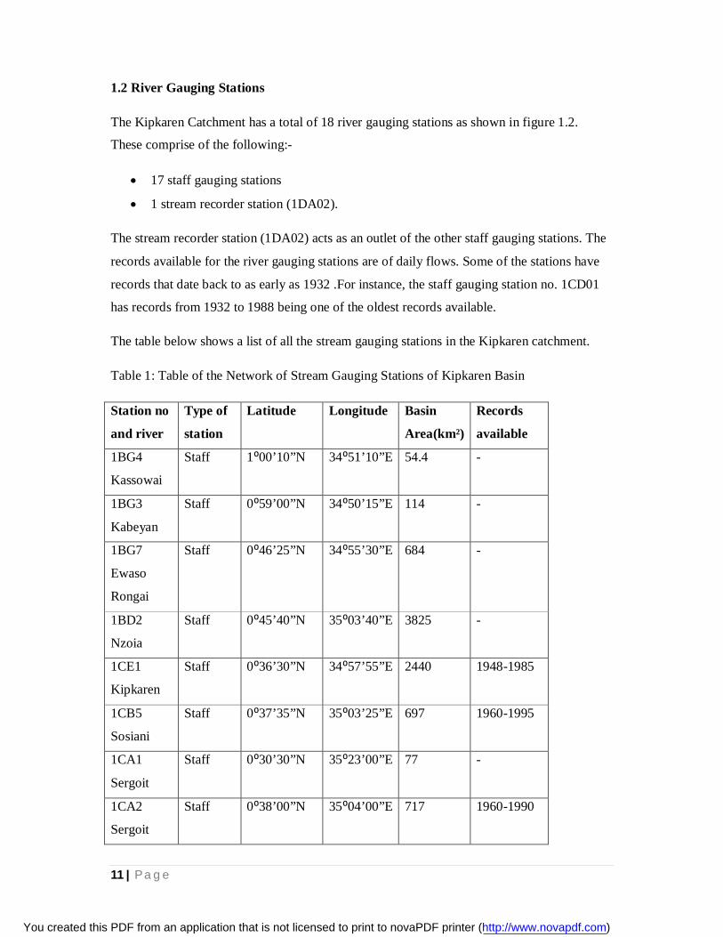
1.2 River Gauging Stations

The Kipkaren Catchment has a total of 18 river gauging stations as shown in figure 1.2.

These comprise of the following:-

17 staff gauging stations

1 stream recorder station (1DA02).

The stream recorder station (1DA02) acts as an outlet of the other staff gauging stations. The

records available for the river gauging stations are of daily flows. Some of the stations have

records that date back to as early as 1932 .For instance, the staff gauging station no. 1CD01

has records from 1932 to 1988 being one of the oldest records available.

The table below shows a list of all the stream gauging stations in the Kipkaren catchment.

Table 1: Table of the Network of Stream Gauging Stations of Kipkaren Basin

Station no

and river

Type of

station

Latitude Longitude

Basin

Area(km²)

Records

available

1BG4

Kassowai

Staff 1⁰00’10”N 34⁰51’10”E 54.4 -

1BG3

Kabeyan

Staff 0⁰59’00”N 34⁰50’15”E 114 -

1BG7

Ewaso

Rongai

Staff 0⁰46’25”N 34⁰55’30”E 684 -

1BD2

Nzoia

Staff 0⁰45’40”N 35⁰03’40”E 3825 -

1CE1

Kipkaren

Staff 0⁰36’30”N 34⁰57’55”E 2440 1948-1985

1CB5

Sosiani

Staff 0⁰37’35”N 35⁰03’25”E 697 1960-1995

1CA1

Sergoit

Staff 0⁰30’30”N 35⁰23’00”E 77 -

1CA2

Sergoit

Staff 0⁰38’00”N 35⁰04’00”E 717 1960-1990



12 | P a g e

Figure 1.3 shows the schematic network of the staff Gauging stations in the Catchment

1.2.1 Rainfall stations

Rainfall stations are those which measure and record daily rainfall only. There are a total of

21 rainfall stations in the Kipkaren River basin, three of which are meteorological stations.

Figure 1.4 shows the network of the Rainfall recorders in the Kipkaren Catchment.

The type of records available is monthly summary of rainfall in the catchment area. The table

below shows a list of all the Rainfall Station Network of the Kipkaren Catchment.

1CB1

Sosiani

Staff 0⁰30’05”N 35⁰17’40”E 298 -

1CB6

Ellegirini

Staff 0⁰28’00”N 35⁰22’25”E 82.9 -

1CB9

Ellegirini

Staff 0⁰27’25”N 35⁰23’20”E 80 -

1CB3

Ellegirini

Staff 0⁰27’05”N 35⁰28’30”E 52 -

1CB7

Nundoroto

Staff 0⁰27’25”N 35⁰22’00”E 167 -

1CB8

Nundoroto

Staff 0⁰26’45”N 35⁰22’00”E 167 1964-1990

1CB2

Kipsanandi

Staff 0⁰25’40”N 35⁰27’50”E 62.2 -

1CD1

Kipkarren

Staff 0⁰24’55”N 35⁰13’25”E 67.3 1932-1988

1CC1

Onyoike

Staff 0⁰23’55”N 35⁰12’00”E 588 1948-1990

1DA2

Nzoia

Recorder 0⁰35’20”N 34⁰48’25”E 8544 1947-1996



13 | P a g e

Table 2: Table of Rainfall Stations Network of the Kipkaren Catchment

Station I.D Station name Latitude Longitude Height(m)

8834013 Kitale , A.D.C

Chorlini

1⁰ 02’N 34⁰ 48’E 1982

8834028 Kitale , Farm 66

Endebes

1⁰ 01’N 34⁰ 54 ’E 1860

8934005 Kitale , Aral

Estate

0⁰ 59’N 34⁰ 50 ’E 1921

8934008 Kitale

,Gloucester Vale

Estate

0⁰ 54’N 34⁰ 55 ’E 1830

8934011 Kitale

,Kapretwa Farm

0⁰ 57’N 34⁰ 49’E 2043

8934033 Kitale ,Kabweya

Estate

0⁰ 59’N 34⁰ 48’E 2165

8934070 Kitale

,Kituwaba

0⁰ 54’N 34⁰ 48’E 2013

8934071 Turbo, Stanely

Estate

0⁰ 42’N 34⁰ 59’E 1905

8934098 Kimilili ,Forest

Station

0⁰ 52’N 34⁰ 41’E 2074

8934113 Kapsakwany

Chief’s Camp

0⁰ 51’N 34⁰ 43 ’E 1830

8934138 Turbo Forest

Station

0⁰ 45’N 34⁰ 58’E 1823

8935010 Kaptagat Forest

Station

0⁰ 22’N 35⁰ 20’E 2440


Land Estate

0⁰ 39’N 35⁰ 04 ’E 1830

8935045 Eldoret ,Kenya

Cooperative

0⁰ 30’N 35⁰ 18 ’E 2074



14 | P a g e

Creameries

8935061 Kipkabus, Tilol 0⁰ 18’N 35⁰ 27’E 2440

8935067 Kaptagat, Mvita

Estate

0⁰ 24’N 35⁰ 29 ’E 2440

8935074 Eldoret Gara

Falls Estate

0⁰ 22’N 35⁰ 15’E 2135

8935076 Turbo Selborne

Estate

0⁰ 39 ’N 35⁰ 01’E 1891

8935117 Kipkabus

,Logarini Estate

0⁰ 19’N 35⁰ 31 ’E 2501

8935133 Eldoret Large

Scale F.T.C

0⁰ 34 ’N 35⁰ 18’E 2134

8935181 Eldoret

Meteorological

Station

0⁰ 32’N 35⁰ 17’E 2120

1.2.2 Meteorological stations

There are three meteorological stations in Kipkaren Catchment. The table of the

meteorological stations is as shown below:

Table 3: List of meteorological stations

Station I.D Station name Latitude Longitude Altitude(m)


Station

0⁰ 45’N 34⁰ 58’E 1823


Land Estate

0⁰ 39’N 35⁰ 04 ’E 1829

8935181 Eldoret

Meteorological

Station

0⁰ 32’N 35⁰ 17’E 2120



15 | P a g e

1.3 Objective

1.3.1 Main Objective

The main objective of the study evaluates the rainfall and stream flow characteristics of the

Kipkaren river basin.

1.3.2 Specific Objectives

To derive the seasonal rainfall pattern of the catchment

To determine the Average rainfall of the catchment

To estimate the Storage required for the catchment

To determine the flow duration and the low flow of the catchment

1.4 Scope of Study

The study only dealt with rainfall and stream flow data from the given period available .The

period of study was majorly influenced by the available data for the particular stations. This

was done by getting the information, and using the data that was available and analysis done

at specific points.



16 | P a g e

CHAPTER TWO

2.0 LITERATURE REVIEW

2.1 Introduction

A drainage basin or river basin or a catchment is an extent of land where water from rain or

snow melts drains downhill into a body of water, such as a river, lake, reservoir, estuary,

wetland, sea or ocean. The drainage basin includes both the streams and rivers that convey

the water as well as the land surfaces from which water drains into those channels, and is

separated from adjacent basins by a drainage divide.

The drainage basin acts like a funnel, collecting all the water within the area covered by the

basin and channeling it into a waterway. Each drainage basin is separated topographically

from adjacent basins by a geographical barrier such as a ridge, hill or mountain, which is

known as a water divide or a watershed.

2.2 Rainfall

Rainfall is known as the main contributor to the generation of surface runoff. Therefore there

is a significant and unique relationship between rainfall and surface runoff. By basic principle

of hydrologic cycle, when rain falls, the first drops of water are intercepted by the leaves and

stems of the vegetation. This is usually referred to as interception storage. Once they reach

the ground surface, the water will infiltrate through the soil until it reaches a stage where the

rate of rainfall intensity exceeds the infiltration capacity of the soil.

The infiltration capacity of soil may vary depending on the soil texture and structure. For

instant, soil composed of a high percentage of sand allows water to infiltrate through it quite

rapidly because it has large, well connected pore spaces. Soils comprising of clay have low

infiltration rates due to their smaller sized pore spaces. However, there is actually less total

pore space in a unit volume of coarse, sandy soil than that of soil composed mostly of clay.

As a result, sandy soils fill rapidly and commonly generate runoff sooner than clay soils.



17 | P a g e

2.2.1 Rainfall Seasonality in the Nzoia Basin.

Across most of the country, rainfall is strongly seasonal, although its pattern, timing and

extent vary greatly from place to place and from year to year. The relatively wet coastal belt

along the Indian Ocean receives 1,000 mm or more rain per year. Most rain falls from April

to July as a result of the southeasterly monsoon. Another moist belt occurs in the Lake

Victoria basin and its surrounding scarps and uplands, mainly due to moist westerly winds

originating over the Atlantic Ocean and Congo Basin. Except immediately adjacent to the

Lake, rainfall occurs reliably from March to November. The upland plateau adjacent to this

area is less influenced by the lake, and rain falls mainly in March-May and July-September.

In much of the central highlands, there is also a bimodal rainfall pattern, with rainy seasons in

March-May and October-December.

Except for the coast and Lake Victoria region, altitude is the main determinant of

precipitation. The high altitude areas in the central Kenya highlands usually have substantial

rainfall, reaching over 2,000 mm per year in parts of the Mau Escarpment. However,

topography also has a major influence, with strong rain shadow effects east of Mt. Kenya and

the Aberdare mountains. Here, even areas higher than 1,800 m may be relatively dry. In the

arid lowlands the peaks of isolated mountains attract cloud and mist, and may support very

different vegetation to that of the surrounding plains. (NRI, 1996)

Mean annual rainfall in Nzoia basin varies from a maximum of 1100-2700 mm and a

minimum of 600-1100mm. The area experiences four seasons in a year as a result of the

inter-tropical convergence zone. There are two rainy seasons and two dry seasons, namely,

short rains (October-December) and the long rains (March-May). The dry seasons occur in

the months of January to February and June to September. However the local relief and

influences of the Lake Victoria modify the regular weather pattern.



18 | P a g e

2.2.2 Rainfall Abstraction

Rainfall abstraction is the component of rainfall that does not turn to direct runoff. This

hydrological abstraction generally comprises the following:-

interception

infiltration

depression storage

evaporation

evapotranspiration

After the initial abstraction is fulfilled, any excess rainfall will become direct runoff. In rural

catchment, interception, evapotranspiration and evaporation do not serve as important factors

for study on runoff and river discharge; however, they are not important in urban catchment.

This is mainly because of its less significant impact. Infiltration depends upon factors such as

tillage, soil structure, antecedent moisture content, infiltrating water quality and the soil air

status. At the early stage, initial abstraction is caused by infiltration, commonly known as the

rainfall that is absorbed by the soil prior to the start of direct runoff; while some assume that

it is the extent of water that penetrates before the infiltration reaches a constant rate. The

approaches to determine initial abstraction are very subjective. (McCuen, 1989).

Until today, there is no definite way to compute the initial abstraction. In common practices,

the initial abstraction is just construed as a part of rainfall losses computed through various

models. Despite that, in many hydrological studies, especially in the humid tropics, initial

abstraction is usually estimated through the linear regression model. The initial abstraction

can then be predicted through the x- intercept of the runoff versus rainfall chart.

2.3 Runoff

Runoff is that part of precipitation, as well as any other flow contribution which appears in

surface streams or rivers of either perennial or intermittent forms. This is the flow collected

from a catchment or drainage basin, and it appears at an outlet of the basin. According to the



19 | P a g e

source from which the flow is derived, runoff may consist of surface runoff, subsurface

runoff and groundwater runoff.

The surface runoff is that part of the runoff which travels over the ground surface and through

channels to reach the basin outlet. The part of surface runoff that flows over the land surface

towards stream/river channels is called overland flow, and after the flows enters a stream, it

joins with other components of flow to form total runoff.

The subsurface runoff is also called as the subsurface flow, interflow, storm seepage or

subsurface storm flow. It is that runoff due to that part of the precipitation which infiltrates

the surface soil and moves laterally through the upper soil zone towards the streams as

ephemeral, shallow, perched groundwater above the main ground water level. Some part of

the subsurface runoff may enter the river promptly, while the remaining part may take a long

time before joining the river flow.

The Groundwater runoff or groundwater flow is that part of the runoff due to deep

percolation of the infiltrated water which has passed into the ground and has become

groundwater, and has been discharged into the river or stream.

For runoff analysis, the total runoff in river channels is generally classified as direct runoff

and base flow. Direct runoff is the runoff which enters the river promptly after the rain or

snow melting. It consists of surface runoff, prompt subsurface runoff and channel

precipitation, while base flow run off is the sustained or fair-weather runoff. It is composed

of ground water runoff and delayed subsurface runoff.

During a run off producing storm, the total runoff may be assumed to consist of excess

precipitation and abstractions. The part of precipitation that contributes entirely to direct

runoff is known as effective precipitation or effective rainfall if only rainfall is involved.



20 | P a g e

2.3.1 Runoff Cycle

The Runoff cycle is comprised of five stages as discussed below.

The first stage relates to the rainless periods just prior to the beginning of rainfall and after an

extended dry period. During this phase, the groundwater table is low and its elevation

continues to decrease gradually. Water is lost through evaporation on land and water surface

and by transpiration from plants.

The second stage relates to initial period of rain. As the rain starts, its amount is divided

among channel precipitation, interception by vegetation, infiltration into the soil, and

temporary retention in surface depressions. The infiltrated water results into a gradual

increase of water in the zone of aeration after the natural storage or field moisture capacity is

satisfied. During this phase, there is little overland flow except on impervious surfaces, while

evaporation and transpiration are slight. Ground water runoff to the streams may or may not

continue, depending on whether the first phase continued until stream flow ceased.

The third stage relates to a continuation of rain at varying intensities .As rain continues, the

capacity of vegetation interception and retention of surface depressions are reached, and the

excess rain becomes a source of runoff and detention storage on land surfaces and in

channels. Overland flow occurs when the net rate of rain exceeds the infiltration rate; but it

may or may not reach the stream or river channel depending on the retention and detention

capacities of the land surface over which it travels. The infiltrated water will saturate the

upper part of the zone of aeration and will then move down to the water table. If rain

continues, the water table will rise and the ground water contribution to the stream flow will

increase.

The fourth stage relates to continuation of rainfall until all natural storage has been satisfied.

The infiltration rate will approach the rate of water transmission through the zone of aeration

to both groundwater table and subsurface runoff. As rain continues, the water table rises

constantly until the groundwater runoff balances the maximum rate of recharge possible and

additional rain results in direct increment of runoff.

The last stage relates to period between the termination of rain and the time when the first

stage is to be reached. It usually involves a long time for channel storage and surface

retention to become depleted. Evapotranspiration is active and infiltration continues. Water in

the zone of aeration is reaching the water table or the river channels .Stream flow is sustained



21 | P a g e

by releasing stored water from the river channels, subsurface flow and groundwater flow. The

water table is rising and then falling when its peak stage is over and the stored water is

diminishing.

It should be noted that, the actual process is more complicated and variable since it is affected

by numerous factors. The above description is just a simplified way of understanding the

runoff cycle.

The figure below show some processes in the runoff cycle.

Fig 2.3.1 Illustration of runoff processes



22 | P a g e

2.3.2 Factors affecting runoff

From the hydrologic point of view, the runoff from a catchment may be considered as a

product of the hydrologic cycle which is influenced by two major groups of factors:-

Climatic factors

Physiographic factors

Climatic factors include mainly the effects of various form and types of precipitation,

interception, evaporation and transpiration, all of which exhibit seasonal variations in

accordance with climatic environment. Physiographic factors may further be classified as into

two types namely: catchment characteristics and channel characteristics.

Catchment characteristics encompass such factors as size, shape and slope of drainage area,

permeability and capacity of groundwater formation, presence of water bodies e.g. swamps

and lakes, and land use. Whereas channel characteristics are related mostly to hydraulic

properties of the channel which govern the movement of river flows and determines the

channel storage capacity. It should however be noted that the above classification of the

factors is by no means exact because many factors are independent to a certain extent.

The following is summary of the major factors that affect runoff:-

i) Vegetation cover

The amount of rain lost to interception storage on the foliage depends on the kind of

vegetation and its growth stage. Values of interception are between 1 and 4 mm. A cereal

crop, for example, has a smaller storage capacity than a dense grass cover. More significant is

the effect the vegetation has on the infiltration capacity of the soil. A dense vegetation cover

shields the soil from the raindrop impact and reduces the crusting effect as described earlier.

In addition, the root system as well as organic matter in the soil increases the soil porosity

thus allowing more water to infiltrate. Vegetation also retards the surface flow particularly on

gentle slopes, giving the water more time to infiltrate and to evaporate. In conclusion, an area

densely covered with vegetation, yields less runoff than bare ground.



23 | P a g e

ii) Slope and catchment size

Investigations on experimental runoff plots (Sharma et al. 1986) have shown that steep slope

plots yield more runoff than those with gentle slopes. In addition, it was observed that the

quantity of runoff decreased with increasing slope length. This is mainly due to lower flow

velocities and subsequently a longer time of concentration (defined as the time needed for a

drop of water to reach the outlet of a catchment from the most remote location in the

catchment). This means that the water is exposed for a longer duration to infiltration and

evaporation before it reaches the measuring point. The same applies when catchment areas of

different sizes are compared. The runoff efficiency (volume of runoff per unit of area)

increases with the decreasing size of the catchment i.e. the larger the size of the catchment the

larger the time of concentration and the smaller the runoff efficiency. Figure 2.4 clearly

illustrates this relationship.

Figure 2.4: Runoff efficiency as a function of catchment size

The purpose of this diagram is to demonstrate the general trend between runoff and

catchment size.



24 | P a g e

iii)Soil type

The infiltration capacity is among others dependent on the porosity of a soil which

determines the water storage capacity and affects the resistance of water to flow into deeper

layers. Porosity differs from one soil type to the other. The highest infiltration capacities are

observed in loose, sandy soils while heavy clay or loamy soils have considerable smaller

infiltration capacities. The infiltration capacity depends furthermore on the moisture content

prevailing in a soil at the onset of a rainstorm. The initial high capacity decreases with time

(provided the rain does not stop) until it reaches a constant value as the soil profile becomes

saturated.

This however, is only valid when the soil surface remains undisturbed. It is well known that

the average size of raindrops increases with the intensity of a rainstorm. In a high intensity

storm the kinetic energy of raindrops are considerable when hitting the soil surface. This

causes a breakdown of the soil aggregate as well as soil dispersion with the consequence of

driving fine soil particles into the upper soil pores. This results in clogging of the pores,

formation of a thin but dense and compacted layer at the surface which highly reduces the

infiltration capacity. This effect, often referred to as capping, crusting or sealing, explains

why in arid and semi-arid areas where rainstorms with high intensities are frequent,

considerable quantities of surface runoff are observed even when the rainfall duration is short

and the rainfall depth is comparatively small. Soils with a high clay or loam content are the

most sensitive for forming a cap with subsequently lower infiltration capacities. On coarse,

sandy soils the capping effect is comparatively small.

The factors affecting runoff generally tend to cause most large catchment areas to behave

differently from most small catchment area on the basis of hydrologic behavior. A distinct

characteristic of small basins is that the effect of overland flow rather than the effect of

channel flow is a dominating factor. Also, small basins are very sensitive both to high

intensity rainfall of short durations and to land use.



25 | P a g e

CHAPTER THREE

3.0 Methodology

The methodology has been split into two phases. The first phase is the methods used for

analysis and the other phase is the collection of data.

3.1 Research Approach

The study deals with point rainfall and runoff data, and therefore uses statistical analysis

method to obtain an estimate of the mean areal rainfall in the area from the rainfall stations

and also the stream flow data.

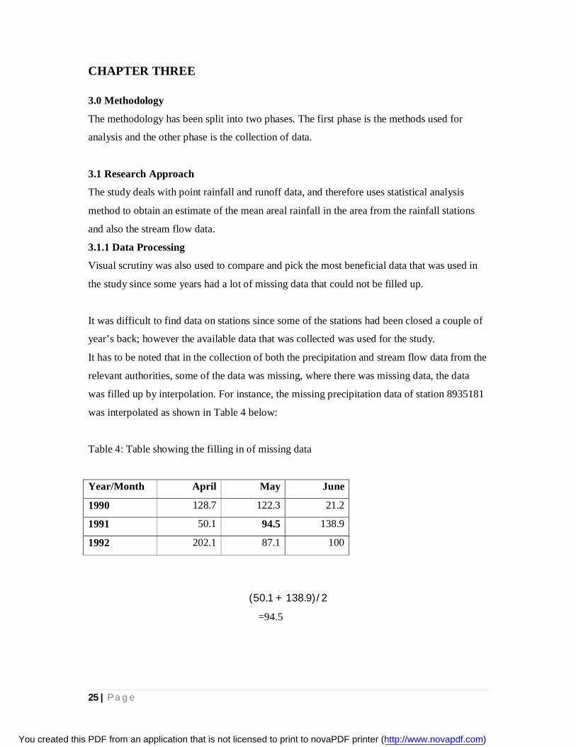
3.1.1 Data Processing

Visual scrutiny was also used to compare and pick the most beneficial data that was used in

the study since some years had a lot of missing data that could not be filled up.

It was difficult to find data on stations since some of the stations had been closed a couple of

year’s back; however the available data that was collected was used for the study.

It has to be noted that in the collection of both the precipitation and stream flow data from the

relevant authorities, some of the data was missing, where there was missing data, the data

was filled up by interpolation. For instance, the missing precipitation data of station 8935181

was interpolated as shown in Table 4 below:

Table 4: Table showing the filling in of missing data

Year/Month April May June

1990 128.7 122.3 21.2

1991 50.1 94.5 138.9

1992 202.1 87.1 100

(50.1 + 138.9)/2

=94.5



26 | P a g e

3.1.2 Rainfall Analysis

3.1.2 .1 Determination of Seasonal Rainfall patterns

The average rainfall in each month for the whole record of the station was obtained; monthly

averages were plotted and compared to observe variations of rainfall in each month.

The local relief modifies the regular weather pattern and therefore the study determines the

mean monthly rainfall over the entire period of study to obtain the seasonal patterns of

rainfall in the Kipkaren catchment. The monthly rainfall for the whole period of study i.e.

1980-2013 (33 years) was summed up and then divided by the total number of years for the

period of study to give the Normal value e.g. March data for all years was summed up and

divided by 33 to give the average March data.

3.1.2.2 Determination of the Average Rainfall

There are several methods used to determine the average rainfall at a station. These include:

Thiessens Method

Isohyetal Method

Simple Mathematical average or Arithmetic mean

Percent Normal

Hysometric methods

Of the methods listed the two most common methods used are the Thiessens Method and

Isohyetal Method. In this study, the Theissen Polygon Method was used because the local

relief or topography had a minimal change in the contours there was no big difference in the

heights.



27 | P a g e

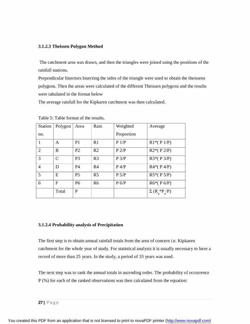
3.1.2.3 Theissen Polygon Method

The catchment area was drawn, and then the triangles were joined using the positions of the

rainfall stations.

Perpendicular bisectors bisecting the sides of the triangle were used to obtain the theissens

polygons. Then the areas were calculated of the different Theissen polygons and the results

were tabulated in the format below

The average rainfall for the Kipkaren catchment was then calculated.

Table 5: Table format of the results.

Station

no.

Polygon Area Rain Weighted

Proportion

Average

1 A P1 R1 P 1/P R1*( P 1/P)

2 B P2 R2 P 2/P R2*( P 2/P)

3 C P3 R3 P 3/P R3*( P 3/P)

4 D P4 R4 P 4/P R4*( P 4/P)

5 E P5 R5 P 5/P R5*( P 5/P)

6 F P6 R6 P 6/P R6*( P 6/P)

Total P Σ (Rn*P

n/P)

3.1.2.4 Probability analysis of Precipitation

The first step is to obtain annual rainfall totals from the area of concern i.e. Kipkaren

catchment for the whole year of study. For statistical analysis it is usually necessary to have a

record of more than 25 years. In the study, a period of 33 years was used.

The next step was to rank the annual totals in ascending order. The probability of occurrence

P (%) for each of the ranked observations was then calculated from the equation:



28 | P a g e

푃 = 푚/(푛 + 1)

Where:

P = probability in % of the observation of the rank m

m = the rank of the observation

N = total number of observations used

The next step is to plot the ranked observations against the corresponding probabilities. For

this purpose normal probability paper was used .Finally a curve is fitted to the plotted

observations in such a way that the distance of observations above or below the curve should

be as close as possible to the curve. The curve may be a straight line.

From this curve it is now possible to obtain the probability of occurrence or exceedance of a

rainfall value of a specific magnitude. Inversely, it is also possible to obtain the magnitude of

the rain corresponding to a given probability.

3.2 Streamflow Analysis

3.2.1 Flow Duration Analysis

A flow duration curve is a plot of discharge vs. percent of time that a particular discharge was

equaled or exceeded. The area under the flow duration curve (with arithmetic scales) gives

the average daily flow, and the median daily flow is the 50% value. It is useful to graph the

data on probability paper.

The available records were analyzed to develop a flow duration curve. It is a cumulative

frequency curve that represents the flow characteristics of a stream throughout the range of

river flows or discharges. It is used in determining the percent of time specified discharges

are equalled or exceeded during a given period.



29 | P a g e

The year of record must be complete for analysis; however these may not be in consecutive

years; the physical conditions in the basin such as artificial storage, diversions and other

manmade influences must essentially be the same during the period of flow analyzed.

Analysis period for assessment - The period selected can either be daily, weekly or monthly

flows in a given period of record. The results of analysis can be used to show the

characteristics of flows when time unit is very short, i.e. daily rather than monthly or annual

and to estimate the percent of time that a specified discharge will be equalled or exceeded in

the future if a reasonable long record of flows is available.

The mid-pts were plotted against Cumulative Probability on Log Probability paper

The value 95% low flow was obtained using the x value of (100 – 95) % = 5%. This is the

value of flow which will be equaled or exceeded 95% of the Time or if the river used for

water supply, the supply would be available 95% of the time; there is a chance of 5% failure.

Note that, usually for an Urban centre, 99% probability is used or maximum probable

precipitation is used.

3.2.2 Low flow analysis

It is used to assess the low flows in the source of water. If adequate and appropriate records

are available it provides a very accurate assessment of low flows.

A low flow frequency analysis evaluates the probability of lows occurring and remaining

below a specified (low) design threshold for a given length of time. Customarily the analysis

is carried out with regard to the minimum discharge aggregated over a period of days in each

year –the minimum discharges are derived from daily flow series.

The analysis requires independent low flow values. Generally the daily, monthly values are

not independent. The daily values should therefore not be used for this analysis; monthly data

may be used but it must be made sure that the values are not dependent. Annual values are

generally acceptable for this analysis. It is very important that the data available is adequate,

generally over 25 year records.

The low flow values are arranged in ascending order; they are ranked (m), Probabilities are

assigned using plotting position, (m/N+1) where N is the Total number of values; the flow

data and the corresponding probabilities are plotted on Log probability paper. The low flow

with the accepted probability of failure is obtained from the graph.



30 | P a g e

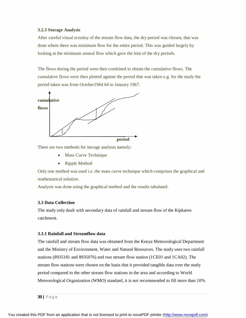
3.2.3 Storage Analysis

After careful visual scrutiny of the stream flow data, the dry period was chosen, that was

done where there was minimum flow for the entire period. This was guided largely by

looking at the minimum annual flow which gave the hint of the dry periods.

The flows during the period were then combined to obtain the cumulative flows. The

cumulative flows were then plotted against the period that was taken e.g. for the study the

period taken was from October1964 64 to January 1967.

cumulative

flows

period

There are two methods for storage analysis namely:

Mass Curve Technique

Ripple Method

Only one method was used i.e. the mass curve technique which comprises the graphical and

mathematical solution.

Analysis was done using the graphical method and the results tabulated.

3.3 Data Collection

The study only dealt with secondary data of rainfall and stream flow of the Kipkaren

catchment.

3.3.1 Rainfall and Streamflow data

The rainfall and stream flow data was obtained from the Kenya Meteorological Department

and the Ministry of Environment, Water and Natural Resources. The study uses two rainfall

stations (8935181 and 8935076) and two stream flow station (1CE01 and 1CA02). The

stream flow stations were chosen on the basis that it provided tangible data over the study

period compared to the other stream flow stations in the area and according to World

Meteorological Organization (WMO) standard, it is not recommended to fill more than 10%



31 | P a g e

of missing data. The rainfall stations were chosen on the basis of their distance from the

stream flow station.

Table 6: Rainfall and stream flow stations used in this study

STATION NO STATION I.D STATION NAME LONGITUDE LATITUDE

1 8935181 Eldoret

Meteorological

Station

35⁰ 17’E 0⁰ 32’N

2 8935076 Turbo Selborne

Estate

35⁰ 01’E 0⁰ 39 ’N

3 1CE01 0⁰36’30”N 34⁰57’55”E

4 1CA02 0⁰38’00”N 35⁰04’00”E



32 | P a g e

CHAPTER FOUR

4.0 ANALYSIS AND DISCUSSION

4.1 RAINFALL ANALYSIS AND DISCUSSION

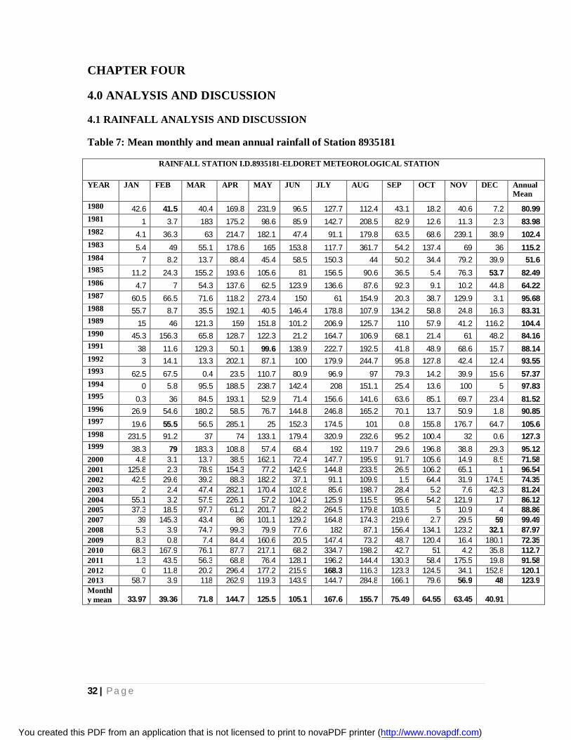
Table 7: Mean monthly and mean annual rainfall of Station 8935181

RAINFALL STATION I.D.8935181-ELDORET METEOROLOGICAL STATION

YEAR JAN FEB MAR APR MAY JUN JLY AUG SEP OCT NOV DEC Annual Mean

1980 42.6 41.5 40.4 169.8 231.9 96.5 127.7 112.4 43.1 18.2 40.6 7.2 80.99 1981 1 3.7 183 175.2 98.6 85.9 142.7 208.5 82.9 12.6 11.3 2.3 83.98 1982 4.1 36.3 63 214.7 182.1 47.4 91.1 179.8 63.5 68.6 239.1 38.9 102.4 1983 5.4 49 55.1 178.6 165 153.8 117.7 361.7 54.2 137.4 69 36 115.2 1984 7 8.2 13.7 88.4 45.4 58.5 150.3 44 50.2 34.4 79.2 39.9 51.6 1985 11.2 24.3 155.2 193.6 105.6 81 156.5 90.6 36.5 5.4 76.3 53.7 82.49 1986 4.7 7 54.3 137.6 62.5 123.9 136.6 87.6 92.3 9.1 10.2 44.8 64.22 1987 60.5 66.5 71.6 118.2 273.4 150 61 154.9 20.3 38.7 129.9 3.1 95.68 1988 55.7 8.7 35.5 192.1 40.5 146.4 178.8 107.9 134.2 58.8 24.8 16.3 83.31 1989 15 46 121.3 159 151.8 101.2 206.9 125.7 110 57.9 41.2 116.2 104.4 1990 45.3 156.3 65.8 128.7 122.3 21.2 164.7 106.9 68.1 21.4 61 48.2 84.16 1991 38 11.6 129.3 50.1 99.6 138.9 222.7 192.5 41.8 48.9 68.6 15.7 88.14 1992 3 14.1 13.3 202.1 87.1 100 179.9 244.7 95.8 127.8 42.4 12.4 93.55 1993 62.5 67.5 0.4 23.5 110.7 80.9 96.9 97 79.3 14.2 39.9 15.6 57.37 1994 0 5.8 95.5 188.5 238.7 142.4 208 151.1 25.4 13.6 100 5 97.83 1995 0.3 36 84.5 193.1 52.9 71.4 156.6 141.6 63.6 85.1 69.7 23.4 81.52 1996 26.9 54.6 180.2 58.5 76.7 144.8 246.8 165.2 70.1 13.7 50.9 1.8 90.85 1997 19.6 55.5 56.5 285.1 25 152.3 174.5 101 0.8 155.8 176.7 64.7 105.6 1998 231.5 91.2 37 74 133.1 179.4 320.9 232.6 95.2 100.4 32 0.6 127.3 1999 38.3 79 183.3 108.8 57.4 68.4 192 119.7 29.6 196.8 38.8 29.3 95.12 2000 4.8 3.1 13.7 38.5 162.1 72.4 147.7 195.9 91.7 105.6 14.9 8.5 71.58 2001 125.8 2.3 78.9 154.3 77.2 142.9 144.8 233.5 26.5 106.2 65.1 1 96.54 2002 42.5 29.6 39.2 88.3 182.2 37.1 91.1 109.9 1.5 64.4 31.9 174.5 74.35 2003 2 2.4 47.4 282.1 170.4 102.8 85.6 198.7 28.4 5.2 7.6 42.3 81.24 2004 55.1 3.2 57.5 226.1 57.2 104.2 125.9 115.5 95.6 54.2 121.9 17 86.12 2005 37.3 18.5 97.7 61.2 201.7 82.2 264.5 179.8 103.5 5 10.9 4 88.86 2007 39 145.3 43.4 86 101.1 129.2 164.8 174.3 219.6 2.7 29.5 59 99.49 2008 5.3 3.9 74.7 99.3 79.9 77.6 182 87.1 156.4 134.1 123.2 32.1 87.97 2009 8.3 0.8 7.4 84.4 160.6 20.5 147.4 73.2 48.7 120.4 16.4 180.1 72.35 2010 68.3 167.9 76.1 87.7 217.1 68.2 334.7 198.2 42.7 51 4.2 35.8 112.7 2011 1.3 43.5 56.3 68.8 76.4 128.1 196.2 144.4 130.3 58.4 175.5 19.8 91.58 2012 0 11.8 20.2 296.4 177.2 215.9 168.3 116.3 123.3 124.5 34.1 152.8 120.1 2013 58.7 3.9 118 262.9 119.3 143.9 144.7 284.8 166.1 79.6 56.9 48 123.9 Monthly mean 33.97 39.36 71.8 144.7 125.5 105.1 167.6 155.7 75.49 64.55 63.45 40.91



33 | P a g e

From the table above it can be clearly seen that the period with the heaviest amount of rainfall was 1998 with an annual mean rainfall of 127.3 mm. It can also be seen that the period with the least amount of rainfall was 1984 with an annual mean of 51.6mm.

4.1.1 Determination of Seasonal Rainfall patterns

Figure 4.1.1: Seasonal rainfall pattern of station no.8935181

From the figure above, it can be shown that the area has two rainy seasons and one dry season. The

dry season occurs from November to February whereas the rainy season occurs from March to May

and July to September. The climate is characterized by a regime of two rainy seasons per year

occurring generally in March to May and in August to October (The months of April/May

have the highest rainfall followed by July and then August.

0

2040

60

80100

120

140160

180

JAN FEB MAR APR MAY JUN JUL AUG SEPT OCT NOV DEC

Rain

fall(

mm

)

Months

Seasonal Rainfall Pattern

Mean monthly Rainfall



34 | P a g e

Table 8: Table of the Annual Total Rainfall of station I.D.8935181-Eldoret Meteorological Station

YEAR Annual Total RANK(m) P=m/(n+1) Percentage (%) 1984 619.2 1 0.0294 2.94 1993 688.4 2 0.0588 5.88 1986 770.6 3 0.0882 8.82 2000 858.9 4 0.1176 11.8 2009 868.2 5 0.1471 14.7 2002 892.2 6 0.1765 17.6 1980 971.9 7 0.2059 20.6 2003 974.9 8 0.2353 23.5 1995 978.2 9 0.2647 26.5 1985 989.9 10 0.2941 29.4 1988 999.7 11 0.3235 32.4 1981 1007.7 12 0.3529 35.3 1990 1009.9 13 0.3824 38.2 2004 1033.4 14 0.4118 41.2 2008 1055.6 15 0.4412 44.1 1991 1057.7 16 0.4706 47.1 2005 1066.3 17 0.5 50 1996 1090.2 18 0.5294 52.9 2011 1099 19 0.5588 55.9 1992 1122.6 20 0.5882 58.8 1999 1141.4 21 0.6176 61.8 1987 1148.1 22 0.6471 64.7 2001 1158.5 23 0.6765 67.6 1994 1174 24 0.7059 70.6 2007 1193.9 25 0.7353 73.5 1982 1228.6 26 0.7647 76.5 1989 1252.2 27 0.7941 79.4 1997 1267.5 28 0.8235 82.4 2010 1351.9 29 0.8529 85.3 1983 1382.9 30 0.8824 88.2 2012 1440.8 31 0.9118 91.2 2013 1486.8 32 0.9412 94.1 1998 1527.9 33 0.9706 97.1

Figure 4.1.2 shows the probability plot of the annual total rainfall of Station 8935181.

From the graph, it is seen that for the probability of 50%,the total annual precipitation is 1100mm for the period of 1980 to 2013 whereas for 5% of precipitation will be 60mm.The 95% of precipitation will be 1400mm.



35 | P a g e

Table 9: Mean monthly and mean annual rainfall of Station no.8935076

RAINFALL STATION I.D.8935076-TURBO SELBORNE ESTATE

YEAR JAN FEB MAR APR MAY JUN JLY AUG SEP OCT NOV DEC MEAN ANNUAL

1980 16.4 1.4 51 177.8 333.3 207.3 162.7 149.1 90.2 31.4 30.4 7.4 104.87

1981 8.6 37.6 274.6 268 137.9 119 145.5 232.3 150 50.8 5.6 22.9 121.07

1982 97.3 20.6 48.2 187.5 281.4 169.8 148.3 287.6 94.2 112.9 215.4 20.3 140.29

1983 40.2 17.5 90 137.5 200.3 148 153.3 231.9 130.8 156.7 54.1 56.7 118.08 1984 14 8.3 22.3 96.7 222.3 159.7 292.1 204 145.5 46.8 65.2 47.5 110.37

1985 32 58 154.5 203.2 295.1 128.3 224.9 193.6 55.6 53.1 136.9 7.5 128.56 1986 6 10 97.6 230.5 190.9 131.2 164.1 91.2 131.7 32.8 7.1 83.6 98.058

1987 37.7 48.3 144 166.6 243.5 155.7 73.3 214.7 46 115.5 178.5 12.6 119.7 1988 57 34.8 24.7 286.3 161.9 110.8 246.6 145.4 229.5 91.5 22.3 4.5 117.94

1989 6.7 42.2 80.4 154.3 145.3 118.7 179.6 188.9 99.9 139.2 52.2 94.6 108.5

1990 50.6 63.9 100.3 224.5 182.8 58.2 149.4 265.9 85.2 71 51.7 54.4 113.16

1991 36.7 26.4 117.1 76.2 164.6 218 209.5 188.3 84 116.9 18.5 17 106.1 1992 17.6 48.7 80.4 200.7 159.1 119.3 446.4 291.7 262.9 65.7 0.3 44.1 144.74

1993 84.2 121.6 119.2 160.1 309.9 228 72 167.8 138.1 11.2 73.4 88.1 131.13

1994 2.1 30.8 114.5 199.2 307.3 127.5 147.5 231.4 119.7 42 135.4 0 121.45

1995 28.8 60.4 113.2 196.4 110.8 219.1 232.4 167.6 125.1 97 125.9 22.1 124.9

1996 71.9 88.1 148.4 120.7 145.6 109.4 151.5 133.2 77.7 95.1 79.2 8.6 102.45

1997 17.8 0 70.5 234.8 69.2 61.2 163.3 135.9 13 194.5 189.9 75.4 102.13

1998 102.6 76.1 12 126.6 293.1 32 327.1 240.5 186.6 365.3 6.8 0 147.39

1999 20.4 1.9 255.1 87.3 79.7 128.6 65.9 158.3 40.8 196.6 32.7 33.3 91.717

2000 0 0 29 108.4 191.6 217.8 110.5 319.8 114.1 134.3 27.5 28.1 106.76

2001 174.6 3.9 141.2 286 255.9 128.8 125.6 260.8 76.1 127.9 57.7 9.3 137.32 2002 17.4 0 49.3 59.5 60.2 39.9 70.5 20.2 2.4 12.9 13.6 82 35.658 2003 0 11.5 17.3 47.3 65.4 54.2 58.1 41.8 43.2 9.6 0 2 29.2

Monthly Mean 39.19 33.83 98.12 168.17 191.96 132.94 171.67 190.08 105.93 98.78 65.85 34.25



36 | P a g e

Figure 4.1.3: Seasonal rainfall pattern of Station no. 8935076

Taking another meteorological station in the catchment (8935076),this to compare the results with the station 8935181. It was seen that it produced the same seasonal pattern as we found out. From figure 4.1.3 it can be seen that there are two rainy seasons and one dry season. The rainy seasons were from March to May and July to October while the dry season was from November to February.

0

50

100

150

200

250

JAN FEB MAR APR MAY JUN JLY AUG SEPT OCT NOV DEC

Rain

fall(

mm

)

Months

Mean Annual Rainfall

Mean monthly Rainfall



37 | P a g e

Table 10: Table of the Annual Rainfall of Station No.8935076-Turbo Selborne Estate

Year Annual Total Rank(m) P=m/(n+1) Percentage (%) 2003 350.4 1 0.04 4 2002 427.9 2 0.08 8 1999 1100.6 3 0.12 12 1986 1176.7 4 0.16 16 1997 1225.5 5 0.2 20 1980 1258.4 6 0.24 24 1996 1271 7 0.28 28 1991 1273.2 8 0.32 32 2000 1281.1 9 0.36 36 1989 1315.5 10 0.4 40 1984 1324.4 11 0.44 44 1990 1344.3 12 0.48 48 1995 1401.8 13 0.52 52 1988 1415.3 14 0.56 56 1983 1417 15 0.6 60 1987 1436.4 16 0.64 64 1981 1452.8 17 0.68 68 1994 1457.4 18 0.72 72 1985 1542.7 19 0.76 76 1993 1595.2 20 0.8 80 2001 1647.8 21 0.84 84 1982 1683.5 22 0.88 88 1992 1736.9 23 0.92 92 1998 1768.7 24 0.96 96

Figure 4.1.5 in page 30(a) shows the probability plot of the annual total rainfall of Station 8935076.

From the figure 4.1.5, it is seen that for the probability of 50%, the total annual precipitation is 1400mm for the period of 1980 to 2003 whereas 95% of precipitation will be 1800mm.



38 | P a g e

4.1.4: Determination of average rainfall by use of Theissen polygon method

Table 11: Theissen Polygon method of finding average rainfall

Gauge No. Polygon Area(km2) Precipitation(mm) Weighted Average 1 A 1009.375 127.2 0.312077 39.696 2 B 325 134.61 0.100483 13.526 3 C 481.25 101.6 0.148792 15.117 4 D 296.875 101.63 0.091787 9.3284 5 E 331.25 126.35 0.102415 12.94 6 F 90.625 122.04 0.028019 3.4195 7 G 362.5 122.05 0.112077 13.679 8 H 243.75 126.81 0.075362 9.5567 9 I 93.75 116.06 0.028986 3.3641

Total 3234.375 120.63

Figure 4.1.9 shows how the Theissen polygon method was done.

By using the Theissen polygon method, the average rainfall in the Kipkaren Catchment was found out to be 120.63 mm.



39 | P a g e

4.2 Stream flow analysis

Table 12: Monthly Summary of the Flow (cumecs) of Gauging Station 1CE01

YEAR JAN FEB MAR APR MAY JUN JULY AUG SEPT OCT NOV DEC Mean Max Min

1954 0.047 0.01 0.001 0.103 1.801 2.227 5.257 17.39 20.49 3.327 0.58 0.501 4.31 20.49 0.001

1955 0.065 0.2 0.035 0.094 0.096 0.231 1.885 43.09 42.9 11.58 2.525 1.501 8.68 43.09 0.035

1956 4.428 1.109 0.223 1.483 3.73 2.532 11.14 50.8 28.93 6.209 1.864 0.76 9.43 50.8 0.223

1957 0.219 0.216 0.264 0.214 2.269 7.525 4.498 10.29 3.758 0.502 0.4 0.22 2.53 10.29 0.214

1958 0.083 0.381 0.103 0.057 1.706 2.566 9.087 18.95 15.27 13.68 1.312 0.635 5.32 18.95 0.057

1959 0.157 0.055 0.183 0.287 1.37 0.894 2.588 6.616 9.136 4.292 1.92 1.181 2.39 9.136 0.055

1960 0.247 0.075 0.253 0.606 1.737 0.992 2.229 9.335 13.02 2.531 1.226 0.346 2.72 13.02 0.075

1961 0.106 0.043 0.031 0.109 0.422 0.938 1.358 26.46 17.34 8.221 70.34 38.27 13.6 70.34 0.031

1962 18.536 4.311 1.705 2.02 16.008 6.2 8.379 28.85 27.76 5.69 3.615 1.54 10.4 28.85 1.54

1963 1.182 0.665 0.624 6.455 43.418 12.23 9.251 27.7 12.52 3.159 2.12 24.88 12 43.42 0.624

1964 3.724 1.02 1.039 4.075 3.677 1.732 16.27 75.67 37.11 20.18 5.199 2.439 14.3 75.67 1.02

1965 1.434 0.469 0.357 0.497 0.763 0.243 0.337 0.879 0.237 0.553 0.824 0.213 0.57 1.434 0.213

1966 0.053 0.034 0.031 3.015 1.857 0.866 1.923 9.956 16.92 1.782 0.839 0.167 3.12 16.92 0.031

1967 0.023 0.012 0.007 0.228 18.961 5.912 31.71 28.67 13.54 6.9 4.384 6.968 9.78 31.71 0.007

1968 0.324 0.798 1.827 4.673 10.449 4.662 5.441 27.3 3.158 1.369 0.439 5.332 5.48 27.3 0.324

1969 1.007 1.177 1.048 0.508 2.062 0.862 1.842 4.34 7.174 1.953 1.08 0.508 1.96 7.174 0.508

1970 1.072 1.26 0.791 3.916 10.014 5.363 5.287 32.3 27.09 9.275 3.549 1.652 8.46 32.3 0.791

1971 0.891 0.476 0.195 0.341 1.251 3.939 12.28 25.06 18.08 8.733 2.77 1.659 6.31 25.06 0.195

1972 1.21 1.393 0.427 0.256 1.628 3.5 13.39 16.65 6.899 4.324 9.28 5.088 5.34 16.65 0.256

1973 1.632 0.799 0.301 0.133 0.535 1.295 0.999 7.495 7.72 3.232 1.961 0.688 2.23 7.72 0.133

1974 0.318 0.126 0.199 0.597 0.634 0.942 4.684 8.297 8.02 2.435 0.829 0.302 2.28 8.297 0.126

1975 0.124 0.056 0.092 0.756 3.282 6.725 10.53 65.89 41.91 19.41 4.807 2.389 13 65.89 0.056

1976 1.013 0.485 0.238 0.358 1.3 1.281 4.842 5.199 8.603 1.501 0.876 0.407 2.18 8.603 0.238

1977 0.344 0.289 0.146 7.275 78.036 40.94 72.22 69.27 39.01 35.79 129.1 45.47 43.2 129.1 0.146

1978 22.268 21.31 52.502 41.58 26.054 19.1 52.12 84.2 74.99 35.53 20.01 14.31 38.7 84.2 14.31

1979 8.453 22.02 12.785 14.72 14.766 18.01 23.61 42.27 15.83 8.533 4.934 3.162 15.8 42.27 3.162

1980 1.895 1.55 1.351 4.51 16.721 12.95 28.1 18.13 13.4 5.412 3.83 2.256 9.18 28.1 1.351

1981 1.462 1.22 4.24 35.97 24.971 13.27 24.62 67.17 43.85 21.99 10.15 5.402 21.2 67.17 1.22

1982 3.157 2.326 1.503 6.997 18.538 21.19 11.26 30.18 18.69 10.9 30.61 41.25 16.4 41.25 1.503

1983 4.858 6.867 4.043 4.157 8.417 9.85 17.5 60.22 66.45 45.58 18.23 8.644 21.2 66.45 4.043

1984 4.551 3.017 1.885 2.357 2.105 2.838 5.634 5.971 4.798 2.603 2.282 1.75 3.32 5.971 1.75

M.M.F 2.7382 2.38 2.8525 4.786 10.277 6.833 12.91 29.83 21.44 9.909 11.03 7.093 MAX.FLOW 22.268 22.02 52.502 41.58 78.036 40.94 72.22 84.2 74.99 45.58 129.1 45.47 MIN.FLOW 0.023 0.01 0.001 0.057 0.096 0.231 0.337 0.879 0.237 0.502 0.4 0.167



40 | P a g e

4.2.1 STATISTICAL FLOW DURATION ANALYSIS OF 1CE01-1954-1984

Table 13: Statistical Flow Duration Analysis

Classes Mid-pt Tally Freq(f) C.F P=m/(n+1) 0.001-0.01 0.0055 III 3 3 0.008 0.01-0.05 0.03 IIII III 8 11 0.03 0.05-0.1 0.075 IIII IIII 10 21 0.056 0.1-0.2 0.15 IIII IIII IIII 14 35 0.094 0.2-0.3 0.25 IIII IIII IIII II 17 52 0.14 0.3-0.4 0.35 IIII IIII II 12 64 0.172 0.4-0.6 0.5 IIII IIII IIII I 16 80 0.215 0.6-0.8 0.7 IIII IIII II 12 92 0.247 0.8-1.0 0.9 IIII IIII III 13 105 0.282 1.0-2.0 1.5 IIII IIII IIII IIII IIII IIII IIII IIII IIII IIII IIII 54 159 0.427 2.0-3.0 2.5 IIII IIII IIII IIII II 22 181 0.487 3.0-4.0 3.5 IIII IIII IIII IIII 19 200 0.538 4.0-6.0 5 IIII IIII IIII IIII IIII IIII IIII 35 235 0.632 6.0-8.0 7 IIII IIII IIII 15 250 0.672 8.0-10.0 9 IIII IIII IIII III 18 268 0.72 10.0-15.0 12.5 IIII IIII IIII IIII III 23 291 0.782 15.0-20.0 17.5 IIII IIII IIII IIII I 21 312 0.839 20.0-30.0 25 IIII IIII IIII IIII III 23 335 0.901 30.0-40.0 35 IIII IIII 10 345 0.927 40.0-60.0 50 IIII IIII IIII 14 359 0.965 60.0-80.0 70 IIII IIII 10 369 0.992 80.0-100.0 90 I 1 370 0.995 100.0-150.0 125 I 1 371 0.997

From the flow duration curve plotted in Figure 4.1.6, it can be seen that for 5% low flow, the flow will be 0.064cumecs.Tthis means that for 5% low flow less than 0.064 cumecs,95% of the time the flow will be greater than 0.064cumecs.

Since we have Eldoret town as the nearby urban centre, the 99% low flow will be 80 cumecs for the 30 years duration. This is the flow of water that will be available 99% of the time for the supply of water. For Rural Water supply, we use 95% low flow, for this case it will be 42 cumecs. 90% low flow will be 26 cumecs. The 50% low flow gives an average value of the flow for the duration considered as 2.6 cumecs.



41 | P a g e

4.2.2 Low flow analysis and Discussion

Table 14: Statistical Low flow Analysis 1954-1984 (1CE01)

Year Annual Flow Rank(m) P=m/(n+1) Percentage (%) 1955 2.94 1 0.031 3.1 1954 10.527 2 0.063 6.3 1956 14.102 3 0.094 9.4 1959 16.986 4 0.125 13 1961 20.32 5 0.156 16 1960 22.448 6 0.188 19 1963 24.83 7 0.219 22 1964 27.109 8 0.25 25 1957 31.319 9 0.281 28 1962 33.273 10 0.313 31 1966 44.494 11 0.344 34 1958 47.548 12 0.375 38 1973 50.52 13 0.406 41 1967 52.758 14 0.438 44 1969 62.615 15 0.469 47 1971 69.048 16 0.5 50 1965 74.966 17 0.531 53 1975 79.759 18 0.563 56 1978 85.81 19 0.594 59 1979 94.152 20 0.625 63 1968 102.011 21 0.656 66 1974 115.987 22 0.688 69 1970 135.533 23 0.719 72 1972 146.892 24 0.75 75 1976 175.942 25 0.781 78 1977 207.571 26 0.813 81 1980 233.802 27 0.844 84 1983 268.519 28 0.875 88 1981 328.671 29 0.906 91 1984 494.837 30 0.938 94 1982 708.945 31 0.969 97

From the graph plotted in figure 4.1.7 in page 34(a), it can be seen that for 5% low flow will be 9.5 cumecs meaning that for 5% low flow < 9.5 cumecs, 95% of the time the flow will be > 9.5 cumecs.



42 | P a g e

4.2.3 Storage analysis

The Graphical Solution was used on the Station 1CA02 because it had a longer period of the dry periods.

Graphical Method-Station 1CA02

Table 17: Cumulative flow of station 1CA02

Period Flow(cumecs) Cumulative flow(cumecs) Oct-64 4.707 4.707 Nov-64 1.278 5.985 Dec-64 0.777 6.762 Jan-65 0.603 7.365 Feb-65 0.179 7.544

Mar-65 0.108 7.652 Apr-65 0.152 7.804

May-65 0.305 8.109 Jun-65 0.095 8.204 Jul-65 0.176 8.38

Aug-65 0.294 8.674 Sep-65 0.112 8.786 Oct-65 0.079 8.865 Nov-65 0.104 8.969 Dec-65 0.049 9.018 Jan-66 0.039 9.057 Feb-66 0.034 9.091

Mar-66 0.025 9.116 Apr-66 0.906 10.022

May-66 0.99 11.012 Jun-66 0.492 11.504 Jul-66 1.416 12.92

Aug-66 7.153 20.073 Sep-66 7.62 27.693 Oct-66 1.08 28.773 Nov-66 0.75 29.523 Dec-66 0.197 29.72 Jan-67 0.058 29.778 Feb-67 0.052 29.83

Mar-67 0.063 29.893 Apr-67 0.119 30.012

May-67 10.09 40.102 Jun-67 3.728 43.83



43 | P a g e

From the mass curve plotted in page 36(a), the storage required for the various ranges of demand were gotten and tabulated as shown below.

Table 16: Demand and Storage required

Demand(cumecs) Storage Required (cumecs) Volume(m3)

d₁ = 1.0 s1 = 12.3 31,881,600

d₂ =0.8 s2 = 10.1 26,179,200

d3 =0.6 s3 =7.1 18,403,200

d4=0.4 s4 = 4.4 11,404,800

d5=0.7 s5=3.2 8,294,400

d6=1.2 s6=13.4 34,732,800

For instance assuming a demand of 1.2cumecs the storage required will be 13.4 cumecs. This translates to (13.4*86400*30) = 34,732,800 m3.

From the graph (figure 4.1.8) x1 is the time it takes for the storage to be full, this is between March 1966 and September 1966.

At point P, that is the time the storage is empty.



44 | P a g e

CHAPTER FIVE

5.0 CONCLUSIONS AND RECOMMENDATIONS

5.1 Conclusion

The hydrological study of the Kipkaren River Basin has revealed very important results. The

objectives which were set for this study were generally achieved to average extent taking into

account the constraints of missing data sets and inaccurate data. Kipkaren River is one of the

largest tributary on the Nzoia River. The following conclusions have been arrived at after the

analysis of both rainfall and stream flow data obtained:

The catchment has two rainy seasons: the short rain season from August to October

and the long rain season from– March to May. Also from the statistical analysis the

50% average precipitation was found to be 1100mm for station.8935181 and 1400mm

for station 8935076 which was close to 1500 which is the mean annual rainfall for the

catchment area. The average rainfall was also found out to be 120.63mm.

Different storage values have been found out, this can be used to estimate the amount

of storage required if the demand in the township is known, for instance the nearby

town is Eldoret Township, so if the demand is 1.0cumecs storage of 31.9*106m3 can

reserved for the water supply in the Township. To put up a dam, one has to do the

survey on the catchment area and take the nearest gauging station, take the flows and

then probability analysis can be further done here for a longer period of records to get

the best storage required.

In the flow duration analysis it was found out that:

5% low flow 0.064cumecs

5% of the time flow < 0.064cumecs

95% of the time flow > 0.064 cumecs

For urban water supply project the 99% flow available would be 80 cumecs.

It is also apparent that the forest cover has decreased remarkably while in contrast, the

agricultural area has increased. This could be attributed to the cutting of trees in the

forests for various uses such as firewood, timber and clearing for agricultural

purposes. This has an effect on the stream flow since the surface runoff will increase

and there will be high level sedimentation due to the eroded river banks that have

cultivated.



45 | P a g e

5.2 Recommendations

In order to provide a sufficient storage, accurate and up-to –date records should be

used because of the changing demands in the Eldoret region. This may be due to the

population growth, industrial use e.tc

In order to reduce flooding and sedimentation more attention should be paid to land-

use patterns and some control measures should be built i.e. afforestation should be

promoted in the basin as one long term measure of managing floods in the basin.

Although the stream flow may shows an increasing tendency in the short rain season

and decreasing tendency in the long rain season, there is a need to study a longer

period than that considered in this study, for better indications of the trends



46 | P a g e

REFERENCES

Associated Program on Flood Management (APFM) (2004a). Strategy for flood management for Lake Victoria basin, Kenya. Ministry of Water Management and Development. Ben Asher, J. (1988). A review of water harvesting in Israel. Bedient, P.B (2nd Edition), Hydrology and Flood Plain Analysis Chow, ven Te, Maidment, David R. and May (1988). Applied Hydrology. New York. McGraw hill. Chow, ven Te. Handbook of Applied of Applied Hydrology. Wilson E.M (1990) 4th Edition ,Engineering Hydrology Development Planning. A Case Study of Kenya. World Soil Resources Report 71/8. FAO/IIASA, Rome. Elizabeth M-Shaw (1994) 3rd Edition, Hydrology in Practice Gupta (1989). Merged rainfall fields for continuous simulation modeling. Kassam A.H., van Velthuizen H.T., Mitchell A.J.B., Fischer G.W. and Shah M.M. 1991. Soil Erosion and Productivity. Technical Annex 2. A Case Study of Kenya. World Soil Resources Report 71/2. FAO/IIASA, Rome. Linsley Ray .K (1992) Hydrology for Engineers. Linsley RK, Kohler MA, Paulhus JLH, Wallace JS, 1958. Hydrology for engineers. McGraw Hill, New York McCuen H.R (1989). Hydrologic Analysis and Design, New Jersey: Meyer, W. B., and B. L. Turner. 1994. Changes in Land Use and Land Cover: A Global Perspective. Cambridge University Press, Cambridge England; New York, NY, USA. MWRMD. 2004. Ministry of Water Resources Management and Development. Strategy for Flood Management for Lake Victoria Basin, Kenya. National Resource Institute. 2006. Kenya travel guide. Kenya weather Nyadawa, M.O., Karanja, F. and Njoroge, T (2007): Application of GIS-based spatially distributed hydrologic model in Integrated Watershed Management: A case study of Nzoia basin, Kenya. Okoola, R.E. 1996: “Space – Time characteristics of the ITCZ over equatorial East Africa during anomalous rainfall years”. PhD. Thesis. Department of Meteorology, University of Nairobi, Kenya. Onyando J.O., T.C. Sharma (1995). Simulation of direct runoff volumes and peak rates for rural catchment in Kenya. Pegram and Zucchini. (1992). Group-based estimation of missing hydrological data.



47 | P a g e

Ponce (1989). Engineering Hydrology: Principles and Practices Van loon.A, Droogers P. (2006). Water evaluation and planning system, Kitui-Kenya. Western Kenya Community Driven Development & Flood Management. 2009. Flood Management Component (WKCDD&FM) Wikipedia, a: http://www.wikipedia.org/wiki/floods (last accessed January 21, 2014) Wikipedia, b: http://www.wikipedia.org/wiki/River (last accessed February 14, 2014) WRMA (2006): Nzoia River Basin Management Initiative (NRBMI), 2006-2011, Civil Society, learning institutions and communities.


http://www.wikipedia.org/wiki/floods

http://www.wikipedia.org/wiki/River


48 | P a g e

APPENNDIX

APPENDIX A: TABLES APPENDIX B: MAPS



a hydrological study of the kipkaren...

Documents