a hybrid model for timbre perception: quantitative …hiroko/timbre/thesis... · ·...
TRANSCRIPT

A HYBRID MODEL FOR TIMBRE PERCEPTION: QUANTITATIVE
REPRESENTATIONS OF SOUND COLOR AND DENSITY
A DISSERTATION
SUBMITTED TO THE DEPARTMENT OF MUSIC
AND THE COMMITTEE ON GRADUATE STUDIES
OF STANFORD UNIVERSITY
IN PARTIAL FULFILLMENT OF THE REQUIREMENTS
FOR THE DEGREE OF
DOCTOR OF PHILOSOPHY
Hiroko Terasawa
December 2009

c© Copyright by Hiroko Terasawa 2010
All Rights Reserved
ii

I certify that I have read this dissertation and that, in my opinion, it is fully adequate
in scope and quality as a dissertation for the degree of Doctor of Philosophy.
(Jonathan Berger) Principal Adviser
I certify that I have read this dissertation and that, in my opinion, it is fully adequate
in scope and quality as a dissertation for the degree of Doctor of Philosophy.
(Chris Chafe)
I certify that I have read this dissertation and that, in my opinion, it is fully adequate
in scope and quality as a dissertation for the degree of Doctor of Philosophy.
(Julius O. Smith)
Approved for the University Committee on Graduate Studies.
iii

Abstract
Timbre, or the quality of sound, is a fundamental attribute of sound. It is important in differenti-
ating between musical sounds, speech utterances, everyday sounds in our environment, and novel
synthetic sounds.
This dissertation presents quantitative and perceptually valid metrics for sound color and den-
sity, where sound color denotes an instantaneous (or atemporal) spectral energy distribution, and
density denotes the fine-scale temporal attribute of sound. In support of the proposed metrics, a
series of psychoacoustic experiments was performed.
The quantitative relationship between the spectral envelope and subjective perception of com-
plex tones was investigated using Mel-frequency cepstral coefficients (MFCC) as a representation of
sound color. The experiments consistently showed that the MFCC model provides a linear and or-
thogonal coordinate space for human perception of sound color. The statistics for all twelve MFCC
were similar at average correlation (R-squared or R2) of 85%, suggesting that each MFCC contains
perceptually important information. The regression coefficients did suggest, however, the lower-
order Mel-cepstrum coefficients may be more important in human perception than the higher-order
coefficients.
The quantitative relationship between the fine-scale temporal attribute and subjective percep-
tion of noise-like stimuli was investigated using normalized echo density (NED). Regardless of the
sound color of the noise-like stimuli, the absolute difference in NED showed a strong correlation
to the perceived dissimilarity with R2 of 93% on average. The other experiments showed that
NED could represent the density perception in a consistent and robust manner across bandwidths–
static noise-like stimuli having similar NED values were perceived as similar regardless of their
bandwidth. Overall, with these experiments, NED showed a strong linear correlation to human
perception of density, along with robustness in estimating the perceived density across various
bandwidths, demonstrating that NED is a promising model for density perception.
The elusive nature of timbre description has been a barrier to music analysis, speech research,
and psychoacoustics. It is hoped that the metrics presented in this dissertation will form the basis
of a quantitative model of timbre perception.
iv

Acknowledgements
First of all, I would like to thank my advisor, Jonathan Berger, who provided full guidance on this
work with his precise, insightful, and creative advice. While I owe any goodness in this work to
him and the following people, I take full responsibility for its flaws.
I am grateful to my thesis committee members, Chris Chafe, Vinod Menon, Julius O. Smith,
and Ge Wang, for their critical advice in this work. My favorite music teachers, Pauline Oliveros
and Jon Appleton, gave me extremely influential lessons to this work.
I would like to acknowledge my collaborators, mentors, and former advisors who supported me
to pursue my graduate program: Jonathan Abel, Antoine Chaigne, Patty Huang, Kenshi Kishi,
Stephen McAdams, Isao Nakamura, Naotoshi Osaka, Stephen Sano, Malcolm Slaney, Hirotake
Yamazoe, and Tomoko Yonezawa.
I appreciate the indispensable and practical help of writing by Julia Bleakney, Blair Bohannan,
Grace Leslie, Jung-eun Lee, Marjorie Mathews, Jessica Moraleda, Sarah Paden, and Peter Wang.
Jim Beauchamp, Chuck Cooper, Eleanor Selfridge-Field, Evelyne Gayou, Michael Gurevich, Mika
Ito, and Masaki Kubo gave me careful comments on my earlier draft.
These researchers offered me fruitful discussion and essential feedback: Akio Ando, Jean-Julien
Aucturier, Al Bregman, John Chowning, Diana Deutsch, Dan Ellis, Masataka Goto, Pat Hanrahan,
Takafumi Hikichi, Andrew Horner, Kentaro Ishizuka, Veronique Larcher, Ed Large, Dan Levitin,
Max Mathews, Atsushi Marui, Kazuho Ono, Geoffroy Peters, Xavier Rodet, Thomas Rossing,
Jean-Claude Risset, Stefania Serafin, and Shihab Shamma.
I greatly appreciate the assistance from CCRMA and Department of Music staff, including
Debbie Barney, Mario Champagne, Jay Kadis, Sasha Leitman, Fernando Lopez-Lezcano, Tricia
Schroeter, Carr Wilkerson, and Nette Worthy.
I acknowledge the generous support from AES Education Foundation, Banff Centre, CCRMA,
Cite internationale des Arts, France-Stanford Center, IRCAM, IPA Mitoh Project, Stanford Grad-
uate Summer Institute.
Finally, I would sincerely like to thank my friends from and outside CCRMA, my housemates,
my family, and my husband for their offerings–Thank you very much!
v

Contents
Abstract iv
Acknowledgements v
1 Introduction 1
1.1 What is Timbre? . . . . . . . . . . . . . . . . . . . . . . . . . . . . . . . . . . . . . . 2
1.2 The Need and Goal for a Timbre Perception Model . . . . . . . . . . . . . . . . . . . 5
1.3 Sound Color and Density . . . . . . . . . . . . . . . . . . . . . . . . . . . . . . . . . 5
1.4 Prior Work on Sound Color . . . . . . . . . . . . . . . . . . . . . . . . . . . . . . . . 6
1.5 Density, the Missing Fine-Scale Temporal Attribute . . . . . . . . . . . . . . . . . . 7
2 Experiments with Sound Color Perception 9
2.1 Introduction . . . . . . . . . . . . . . . . . . . . . . . . . . . . . . . . . . . . . . . . . 9
2.1.1 Review and Proposals on Sound Color Perception Experiments . . . . . . . . 10
2.1.2 Discussion of MFCC for a Perceptual Sound Color Model . . . . . . . . . . . 11
2.1.3 Experiment Design Overview . . . . . . . . . . . . . . . . . . . . . . . . . . . 13
2.2 MFCC Based Sound Synthesis . . . . . . . . . . . . . . . . . . . . . . . . . . . . . . 14
2.2.1 MFCC . . . . . . . . . . . . . . . . . . . . . . . . . . . . . . . . . . . . . . . . 14
2.2.2 Sound Synthesis . . . . . . . . . . . . . . . . . . . . . . . . . . . . . . . . . . 17
2.3 Experiment 1: Single-Dimension Sound Color Perception . . . . . . . . . . . . . . . . 18
2.3.1 Scope . . . . . . . . . . . . . . . . . . . . . . . . . . . . . . . . . . . . . . . . 18
2.3.2 Method . . . . . . . . . . . . . . . . . . . . . . . . . . . . . . . . . . . . . . . 18
2.3.3 Analysis 1. Linear Regression . . . . . . . . . . . . . . . . . . . . . . . . . . . 21
2.3.4 Analysis 2. Equivalence Test in Pairwise Comparison . . . . . . . . . . . . . 22
2.3.5 Analysis 3. Spectral Centroid Assessment . . . . . . . . . . . . . . . . . . . . 23
2.3.6 Discussion . . . . . . . . . . . . . . . . . . . . . . . . . . . . . . . . . . . . . . 24
2.4 Experiment 2: Two-dimensional Sound Color Perception . . . . . . . . . . . . . . . . 24
vi

2.4.1 Scope . . . . . . . . . . . . . . . . . . . . . . . . . . . . . . . . . . . . . . . . 24
2.4.2 Method . . . . . . . . . . . . . . . . . . . . . . . . . . . . . . . . . . . . . . . 25
2.4.3 Multiple Regression Analysis . . . . . . . . . . . . . . . . . . . . . . . . . . . 28
2.4.4 Discussion . . . . . . . . . . . . . . . . . . . . . . . . . . . . . . . . . . . . . . 31
2.5 Chapter Summary and Future Work . . . . . . . . . . . . . . . . . . . . . . . . . . . 31
3 Explorations of Density 33
3.1 Introduction . . . . . . . . . . . . . . . . . . . . . . . . . . . . . . . . . . . . . . . . . 33
3.2 Normalized Echo Density . . . . . . . . . . . . . . . . . . . . . . . . . . . . . . . . . 37
3.3 Synthesis of Noise Stimuli . . . . . . . . . . . . . . . . . . . . . . . . . . . . . . . . . 38
3.4 Experiment 3: Dissimilarity of Perceptual Density . . . . . . . . . . . . . . . . . . . 39
3.4.1 Scope . . . . . . . . . . . . . . . . . . . . . . . . . . . . . . . . . . . . . . . . 39
3.4.2 Method . . . . . . . . . . . . . . . . . . . . . . . . . . . . . . . . . . . . . . . 39
3.4.3 Analysis . . . . . . . . . . . . . . . . . . . . . . . . . . . . . . . . . . . . . . . 41
3.5 Experiment 4: Density Grouping . . . . . . . . . . . . . . . . . . . . . . . . . . . . . 42
3.5.1 Scope . . . . . . . . . . . . . . . . . . . . . . . . . . . . . . . . . . . . . . . . 42
3.5.2 Method . . . . . . . . . . . . . . . . . . . . . . . . . . . . . . . . . . . . . . . 43
3.5.3 Analysis . . . . . . . . . . . . . . . . . . . . . . . . . . . . . . . . . . . . . . . 44
3.6 Experiment 5: Density Matching . . . . . . . . . . . . . . . . . . . . . . . . . . . . . 45
3.6.1 Method . . . . . . . . . . . . . . . . . . . . . . . . . . . . . . . . . . . . . . . 45
3.6.2 Analysis . . . . . . . . . . . . . . . . . . . . . . . . . . . . . . . . . . . . . . . 47
3.7 Discussion . . . . . . . . . . . . . . . . . . . . . . . . . . . . . . . . . . . . . . . . . . 48
4 Conclusion 50
4.1 Modeling Sound Color . . . . . . . . . . . . . . . . . . . . . . . . . . . . . . . . . . . 50
4.2 Investigating Density . . . . . . . . . . . . . . . . . . . . . . . . . . . . . . . . . . . . 51
4.3 Color of Noises, Density of Sinusoids . . . . . . . . . . . . . . . . . . . . . . . . . . . 52
4.4 Leading to Trajectory . . . . . . . . . . . . . . . . . . . . . . . . . . . . . . . . . . . 52
Bibliography 53
vii

List of Tables
3.1 Perceived density breakpoints expressed in NED and AED . . . . . . . . . . . . . . . 46
3.2 Perceptually matching density expressed in NED and AED . . . . . . . . . . . . . . 48
viii

List of Figures
2.1 Algorithm overview of MFCC . . . . . . . . . . . . . . . . . . . . . . . . . . . . . . 15
2.2 Frequency response of the filterbank used for MFCC . . . . . . . . . . . . . . . . . . 16
2.3 Spectral envelopes generated by varying a single Mel-cepstrum coefficient . . . . . . 19
2.4 Graphical user interface for the experiment . . . . . . . . . . . . . . . . . . . . . . . 21
2.5 Coefficients of determination (R2) from regression analysis of the single-dimensional
sound color experiment . . . . . . . . . . . . . . . . . . . . . . . . . . . . . . . . . . 22
2.6 Spectral centroid of the stimuli used for the single-dimensional sound color experi-
ment . . . . . . . . . . . . . . . . . . . . . . . . . . . . . . . . . . . . . . . . . . . . 24
2.7 Spectral envelopes generated by varying two Mel-cepstrum coefficients . . . . . . . . 26
2.8 Selection of the test pairs for the two-dimensional sound color experiment . . . . . . 27
2.9 Coefficient of determination (R2) from regression analysis of the two-dimensional
sound color experiment . . . . . . . . . . . . . . . . . . . . . . . . . . . . . . . . . . 29
2.10 Regression coefficients from regression analysis of the two-dimensional sound color
experiment . . . . . . . . . . . . . . . . . . . . . . . . . . . . . . . . . . . . . . . . . 30
3.1 Normalized echo density profile of a measured room impulse response . . . . . . . . 38
3.2 Graphical user interface for the dissimilarity test . . . . . . . . . . . . . . . . . . . . 41
3.3 Coefficient of determination (R2) from regression analysis of the perceptual density
experiment . . . . . . . . . . . . . . . . . . . . . . . . . . . . . . . . . . . . . . . . . 42
3.4 Graphical user interface for the density categorization experiment . . . . . . . . . . . 44
3.5 Density grouping: breakpoints to separate three density regions . . . . . . . . . . . . 45
3.6 Perceived density breakpoints across bandwidths . . . . . . . . . . . . . . . . . . . . 45
3.7 Density matching experiment graphical user interface. . . . . . . . . . . . . . . . . . 47
3.8 Perceptually matched static echo patterns . . . . . . . . . . . . . . . . . . . . . . . . 49
ix

Chapter 1
Introduction
“The whole of our sound world is available for music-mode listening, but it probably
takes a catholic taste and a well-developed interest to find jewels in the auditory garbage
of machinery, jet planes, traffic, and other mechanical chatter that constitute our sound
environment. Some of us, and I confess I am one, strongly resist the thought it is
garbage. The more one listens the more one finds that it is all jewels.”
Robert Erickson, Sound Structure in Music [Erickson1975].
“The problem with timbre is that it is the name for an ill-defined wastebasket category.
Here is the much-quoted definition of timbre given by the American Standards Associ-
ation: ‘that attribute of auditory sensation in terms of which a listener can judge that
two sounds similarly presented and having the same loudness and pitch are dissimilar.’
This is, of course, no definition at all.”
Al Bregman, Auditory Scene Analysis[Bregman2001].
1

CHAPTER 1. INTRODUCTION 2
Timbre is an auditory jewelry box.
What we find in this jewelry box are the colors, textures, and shapes of myriad sound materials.
The ANSI definition of timbre[ANSI1976], which Bregman introduced in the above quote, is
often interpreted as double negation: Timbre is the auditory perception of sound, which is neither
pitch nor loudness. This says what timbre is not, rather than what timbre is. And this essentially
catch-all interpretation of the definition could mean that any nameless attribute could fall into the
timbre category. Bregman’s analogy brilliantly captures this implication of the standard definition.
But for those with the ears of “music-mode listening,” it’s time for another analogy, which
captures the richness of timbre.
Timbre is an auditory jewelry box, in which we find art and craft, nature and culture, old and
new, in many materials and designs from around the world. Timbre is something to be enjoyed,
appreciated, and marveled at. Timbre generously allows us to observe and analyze it from various
perspectives. With this work, I wish to help refine the notion of timbre.
1.1 What is Timbre?
What timbre is may not yet be clear with the above definitions. In fact, this is the same question
that researchers and musicians have been asking for a long time.
According to the Oxford English Dictionary, one of the earliest examples in which the word
timbre was used in English literature was in the context of auscultation, in which, a doctor would
be listening to the sounds from the heart or other organs typically using a stethoscope. It was still
a new technology in 1853, when a British medical doctor William Markham translated Abhandlung
uber Perkussion und Auskultation, written in German by Joseph Skoda, into its English edition A
Treatise on Auscultation and Percussion [Skoda1853]:
The voices of individuals, and the sounds of musical instruments, differ, not only in
strength, clearness, and pitch, but (and particularly) in that quality also for which there
is no common distinctive expression, but which is known as the tone, the character, or
timbre of the voice. The timbre of the thoracic, always differs from the timbre of the
oral, voice... A strong thoracic voice partakes of the timbre of the speaking-trumpet.
(Translated by W. O. Markham.)
In this description, Markham uses the words such as quality, character, and tone to describe
timbre, in addition to the analogy to a musical instrument.

CHAPTER 1. INTRODUCTION 3
Even a hundred years after from this introduction, the notion of timbre was still under debate,
as described by Alexander John Ellis, who translated On the sensations of tone by Helmholtz. Ellis
provided an extensive footnote on the choice of this term among options such as timbre, clangtint,
quality of tone, or colour discussing the already existing meanings for each term [Helmholtz1954].
He explains that the term timbre can be fully designated to express this perceptual attribute of
sound because it is an obscure and foreign word, whereas the other terms have specific connotations
for traditional usages in English. This frustration demonstrated by Ellis might be the same kind of
frustration we have today about the definition of timbre, as exhibited by Bregman.
However, I have an impression that even if we do not have an explicit definition, we already hold
some or sufficient, if not plentiful, tacit knowledge [Polanyi1967] about timbre from our experience.
Let me introduce some stories narrated by poet, sound engineer, philosopher, performer, and com-
posers. These anecdotes reflect images, thoughts, and decisions of those working in the domain of
timbre, in which their concern was that of a quality other than pitch and loudness.
Matsuo Basho, Japanese Poet from the 17th century, composed a poem [Keene1955]:
Furu ike ya
kawazu tobikomu
mizu no oto
The ancient pond
A frog leaps in
The sound of water
(Translated by Donald Keene)
In this poem, the sound of splash brings a life to the little frog while emphasizing the surrounding
silence.
Shuji Inoue, the sound engineer of “Howl’s Moving Castle” by Studio Ghibli, works extensively
on environmental sounds [Ida2005]:
Unlike other types of films, which may come with diegetic sounds, animation films have
to start with no sound: we have to prepare not only dialogues, but also the rustle of
clothes and environmental sounds. Of course we could purchase sound libraries, but
works by Studio Ghibli aim for the ultimate reality, so that I went out to anywhere with
microphones. Because the film is set at late 19th century Europe, I went to Marseille and
Colmar in France and recorded footsteps and horse-drawn carriage sounds reflecting on
the stone pavements. I also flew into the middle of mountains in Switzerland, to express
the air unique in Europe. Although not very noticeable, there is always “sound of the

CHAPTER 1. INTRODUCTION 4
air” around us, as environmental sound. By simply adding this sound, the world of
animation suddenly starts to have a deep perspective.
A philosopher specialized in aesthetics and the philosophy of art, Peter Kivy raises questions
about the timbral quality of period instruments referring to the “Roland C-50 classic harpsichord”,
which is an electronic harpsichord [Kivy1995].
What particularly fascinates me about the Roland C-50 is that it includes, among its
many features, the ability to reproduce not only the distinctive plucked harpsichord
tone but, its maker says, “the characteristic click of the jacks resetting,” which, of
course, because the machine possesses neither jacks nor strings, must, like the plucked
tone, be reproduced electronically. In other words, the modern electronic harpsichord
maker has bent every effort to construct an instrument that can make a “noise” the
early harpsichord maker was bending every effort not to make. . . . Our triumph is their
failure.
Brian May, the lead guitarist and songwriter of the British rock band Queen, is known for using
a sixpence coin instead of a plectrum, as he answers in an interview[Bradley2000].
It’s a great help to use the coin as, depending how it’s orientated to the strings, it can
produce a varying amount of additional articulation, and by that I mean when you can
hear just one string peeping through the whole spectrum of the rest of it.
So, if the sixpence is turned parallel to the strings, it’s quite a soft effect, even though
it’s a piece of metal. And if you turn it sideways, the serrated edge changes the sound
quite dramatically. I’ve always preferred the coin to anything else, both for that reason
and because it doesn’t ’give’ between the string and your fingers. Sixpences are very
cheap these days!
Hungarian (later Austrian) composer Gyoergy Ligeti, who is known to have had synesthesia,
states that to him, sounds have color, form, and texture [Ligeti and Bernard1993].
The involuntary conversion of optical and tactile into acoustic sensations is habitual
with me: I almost always associate sounds with color, form, and texture; and form,
color, and material quality with every acoustic sensation.
French composer Pierre Boulez describes blends of timbres in art music after the 19th century
[Boulez1987].
Up to the 19th century, the function of timbre was primarily related to its identity.
. . . With the modern orchestra, the use of instruments is more flexible and their identi-
fication becomes more mobile and temporary. Composing the blending of timbres into

CHAPTER 1. INTRODUCTION 5
complex sound-objects follows from the confronting of established sound hierarchies and
an enriching of the sound vocabulary. The function of timbre in composed sound-objects
is one of illusion and is based upon the technique of fusion.
When these people are deeply concerned about timbre, their sounds may come from musical,
environmental, spoken, or synthesized sounds. The scope of this term timbre is thus broad and
subtle, yet there has not been a widely accepted theory of timbre from such a general perspective.
1.2 The Need and Goal for a Timbre Perception Model
This work, therefore, aims to establish a perceptually valid and quantitative model of timbre which
embodies musical, spoken, and environmental sounds. Such a model will enable us to analyze digital
audio data from various sources (including, but not limited to music, other media content, and the
soundscape of our daily life) and to control timbre in sound synthesis in a perceptually meaningful
way.
Desirably, this timbre perception model will be versatile, robust, and durable. By versatile,
I mean that the model has a very broad scope: the sound to be considered could be musical,
spoken, environmental, or newly invented. By robust, I mean that the model can handle signals of
various characteristics: periodic and aperiodic (stochastic); harmonic and inharmonic; regular and
irregular; dynamic and static. And by durable, I mean that the model can be flexibly applied to
the sounds in the future, not limited to currently known sounds–there will be new and unfamiliar
sounds in the future, and we will be flexibly listening to them, just as we accommodated then-newly
emerging sounds in the past. For a model to be flexibly applicable to currently unknown sounds,
it must be versatile and robust so that it can incorporate any audio signal in any context.
1.3 Sound Color and Density
An inspiring role model for such a timbre perception model would be the sinusoidal model synthesis,
proposed by Quatieri [McAuley and Quatieri1986] and later adopted for musical purposes by Serra
[Serra1989]. This model is unique in its versatility and treatment of stochastic portion in sound.
This model represents a signal as an addition of sinusoids and stochastic portions: the sinusoids have
instantaneously changing frequencies and amplitudes, and the stochastic portions are the residual
after those sinusoids are removed from the signal.
This signal-driven framework is truly versatile and robust–it works for any kind of signal because
it does not presume any physical constraints on a signal. If we analyze a mostly stochastic signal,
the “residual” portion becomes predominant, and the sinusoidal portion becomes very little.

CHAPTER 1. INTRODUCTION 6
With this technique, we can listen to a sound’s stochastic portion and periodic portion separately.
If we analyze a guitar sound with this method, we can hear the periodic motion of the string, with
some shift in pitch, and with rise, sustain and release state in its amplitude apart from the squeaky
friction sound of the finger rubbing the string followed by the string’s nonlinear, onset transient.
The qualities to be heard in these separated signals demonstrate a strong contrast. In my
opinion, when a signal is periodic, a smooth continuum of sinusoids, its spectral attribute becomes
the dominant perceived character, whereas, when a signal is stochastic, a sequence of aperiodic
impulses, its temporal attribute becomes the dominant perceived character.
Let’s name these spectral and temporal attributes sound color and density1 respectively:
• Sound color is an instantaneous (or atemporal) description of spectral energy distribution.
• Density is a description of the fluctuation of instantaneous intensity, in terms of both rapidity
of change and degree of differentiation between sequential instantaneous intensities.
This thesis provides a new set of quantitative representations which translate the above acous-
tical attributes, sound color and density, into linearly scaled perceptual estimates.
1.4 Prior Work on Sound Color
As many researchers viewed the spectrum of a sound and the spectrum of a visual color as being
relevant to each other, the analogy between color in vision and the spectral attribute of a sound has
been prevalent. Helmholtz, in his discussion on the effect of each harmonic’s amplitude of a complex
tone on its timbre, addressed the analogy with the prime colors in vision perception, quoting then-
contemporary scientific experiments on three prime colors and color mixtures [Helmholtz1954].
The phenomena of mixed colours present considerable analogy to those of compound
musical tones, only in the case of coulour the number of sensations reduces to three, and
the analysis of the composite sensations into their simple elements is still more difficult
and imperfect for musical tones.
In addition to the analogy between mixed color and musical tone with complex harmonic structure,
he presented, already in this above quote, the idea of explaining the complex harmonic structure
of musical tone into primary elements.1Word choice for this attribute: Between the two possible terms, texture and density, I chose to use the word
density because (1) density had a narrower range of connotations than texture (the Oxford English Dictionary), and(2) in the context of musical texture, according to Rowell, the analogy for density was specifically thin-dense, wheretexture covers a larger set of analogies over multiple qualitative dimensions (e.g. simple-complex, smooth-rough,thin-dense, focus-interplay, among others) [Rowell1983]. To summarize, the connotations for texture tend to bequalitative and multidimensional, and the connotations for density tend to be quantitative and single-dimensional.For that reason, I considered density is a better choice than texture to specifically describe the fine-scale temporalattribute.

CHAPTER 1. INTRODUCTION 7
Among the later researchers who inherited the concept of sound color, Wayne Slawson, composer
and music theorist, defines sound color as following [Slawson1985]:
Sound color is a property or attribute of auditory sensation; it is not an acoustic prop-
erty. . . . Like visual color, sound color has no temporal aspect. . . . When we say that a
sound color has no temporal aspect, this rules out of consideration all changes in sounds.
That is, a sound may be heard to be changing from one color to another, but the change
itself is not a sound color.
In this definition, Slawson clarifies that sound color belongs purely to the spectral (atemporal)
domain in the dichotomy of spectral vs. temporal attributes, which is a view shared by other
researchers including Plomp [Plomp1976] and Hartmann [Hartmann1997].
However, note that Slawson’s definition of sound color is in the perceptual domain, whereas in
this work, sound color itself is in the acoustical domain. Chapter 2 offers a model for sound color
perception, which translates this acoustical attribute into a linearly scaled estimate of perception,
with supporting data from a series of psychoacoustic experiments.
1.5 Density, the Missing Fine-Scale Temporal Attribute
A spectral analysis often dismisses the fine-scale temporal information of sound. For example, in
the application of the short-time Fourier transform (STFT), we often lose the temporal information
within a window of observation. In theory, we could find the temporal information in the phase of
the complex spectrum of a sound, but in practice, we rarely do so, and we tend to observe only the
power spectrum of the sound. Therefore the information on the fine-scale temporal arrangement is
typically lost in the blur of the power spectrum, leaving it hard to analyze.
As discussed earlier, in his sinusoidal modeling synthesis of musical sounds, Xavier Serra solved
this dilemma by representing a signal as an addition of “sinusoids and noise” (i.e. periodic and
stochastic) [Serra1989]. This model reserves the fine-scale temporal attribute by separating it from
the periodic elements of the signal. This “stochastic” portion of sound is also addressed by Wishart
[Wishart1996]: He introduces “aperiodic grain” as “a large aggregate of brief impulses occurring
in a random or semi-random manner,” which “has a bearing on the particular sonority of sizzle-
cymbals, snare-drums, drum-rolls, the lion’s roar, and even the quality of string sound through
the influence of different weights and widths of bows and different types of hair and rosin on the
nature of bowed excitation.” Although they express and approach the idea differently, both Serra
and Wishart consider that quality of sound which can only be ascribed to the fine-scale temporal
attribute.

CHAPTER 1. INTRODUCTION 8
However, this quality is rarely studied in psychoacoustics: Only a few reports actually discuss
the perception of stochastic signals, such as percussive instruments and impact sounds [Lakatos2000,
Giordano and McAdams2006, Goebl and Fujinaga2008].
Chapter 3 presents a potential model for density perception, which translates the acoustical
attribute of density into a linearly scaled estimate of perception, with the supportive data from a
series of psychoacoustic experiments.

Chapter 2
Experiments with Sound Color
Perception
2.1 Introduction
In this chapter, the perception of sound color is investigated, and a perceptually viable model of
sound color is proposed. Sound color is, as described in chapter 1, the instantaneous (or atemporal)
description of spectral energy distribution of a sound.
Perceptual maps exist for pitch and loudness in the auditory domain, as well as for color in the
visual domain. In each case, a relatively simple model connects physical attributes (mel for pitch,
sone for loudness, and the three cones of the visual system for color) with perceptual judgments.
However, no such model currently exists for sound color.
The perceptual model proposed in this chapter aims for a simple, compact, and yet descriptive
representation of sound color, which allows us to directly and quantitatively estimate our perception
of this attribute; an auditory equivalent to Munsell’s color system [Munsell and Farnum1946]. As
described in the following discussion, the perception of sound color is multidimensional. Therefore,
an important goal of this work is to find a quantitative representation to describe the perceptual
sound color space with a set of perceptually orthogonal axes. In other words, we want to find an
auditory equivalent to primary colors in vision, which explains the mixture of colors as a sum of
independent elements.
It is also desirable that the representation of each primary sound color is quantitatively labeled to
predict human perception in a straightforward, proportional manner. That said, the representation
of sound color should linearly represent the perception of sound color.
9

CHAPTER 2. EXPERIMENTS WITH SOUND COLOR PERCEPTION 10
To summarize, this work aims for a model which represents the multidimensional space of sound
color perception with linear and orthogonal coordinates.1
2.1.1 Review and Proposals on Sound Color Perception Experiments
The perception of sound color is discovered to be multidimensional itself. Plomp studied the effect
of spectral envelopes on human perception [Plomp1976]. In this work, Plomp extracted a single
period from a waveform of the sustained state of musical instrumental sounds of a common pitch. By
repeating the single period, he obtained a static tone of a particular spectral envelope with the least
temporal change; in other words, a set of sounds which differ only in sound color, without temporal
deviations. The subjective dissimilarity judgments of the tones were collected, and the perceived
dissimilarity scores were explained in terms of the principal component analysis of the spectra, which
described the spectra with three orthogonal factors. In this work he found multidimensionality in
the perception of his stimuli set, suggesting multidimensionality in the perception of sound color.
When we look into the results from classic multidimensional scaling studies of musical timbres by
Grey, Wessel, McAdams, and Lakatos [Grey1975, Wessel1979, McAdams et al.1995, Lakatos2000],
there was, among the perceptual dimensions they found, only a single dimension related to the
sound color, which was spectral centroid. The other dimensions, spectral flux and attack time,
were temporal aspects. Unlike Plomp’s study, these studies integrated temporal aspects of timbre,
and succeeded in investigating the perception of more complex and realistic musical tones. However,
the multidimensionality of sound color was not visible. The subjective judgments of sound color
were observed only in a single dimension.
How did the multidimensionality of sound color get lost? It seems that the temporal attribute
of the musical timbres masked out or reduced the attention to the multidimensionality of sound
color, resulting in the reduced dimensionality of the observed sound color perception. The temporal
attributes of sound, both fine-scale and larger-scale, are complex, multidimensional, and possibly
nonlinear. The temporal attributes could deliver substantial effects on timbre perception, while
the effect of sound color could be more subtle. Therefore, in measuring the multidimensionality of
sound color perception, a good approach would be to minimize the temporal variance across stimuli,
so that the pure effect of sound color is measured without the distraction of temporal attributes.
In his study on describing the perceived difference of stimuli with various sound colors with the
three factors from principal components analysis of spectrum, Plomp concluded:1Malcolm Slaney took a very important role in the preliminary studies of sound color, which we reported in the
following papers [Terasawa et al.2005a, Terasawa et al.2005c, Terasawa et al.2005b, Terasawa et al.2006]. AlthoughI extended the framework, revised the experiment design, and newly collected and analyzed the data for the soundcolor experiments included in this thesis, this work still reflects many of his methodologies, ideas, and suggestionsfor the preliminary studies on timbre perception.

CHAPTER 2. EXPERIMENTS WITH SOUND COLOR PERCEPTION 11
In this example, based upon a specific set of stimuli, three factors alone appeared to be
sufficient to describe the differences satisfactorily. This number cannot be generalized.
If we had started from a set of tones differing only in the slope of their sound spectra, a
single factor would have been sufficient. It is also possible to select nine stimuli which
would require, for example, five dimensions to represent their timbres appropriately.
This conclusion says, in other words, that a general model cannot be provided by observing the
perception of only a specific set of sounds. This is, in fact, a common problem in taking a non-
parametric approach.
The limitation of a non-parametric approach is that the resulting model of timbre perception
will depend on the specific selection of sounds included in the data set. For example, if the data
set contains only the instrumental sounds of the western classical orchestra, the resulting model
derived from that data set will be applicable to these instrumental sounds, but may not be ap-
propriate to analyze other types of sounds, such as non-western musical instrument sounds or
computer-generated sounds with unusual timbre. Hajda made an argument on this issue in his
essay [Hajda et al.1997] that non-parametric psychological measurements aid our understanding
of timbre perception but do not necessarily support the formation of a timbre representation or
metric. He argues that while “advances on digital signal processing and non-parametric statistical
methods” aided “the researcher in uncovering previously hidden perceptual structures,” this re-
search was conducted without “attention to first-order methods, namely, assumptions and working
definitions of what it is that is being studied” or “standard hypothesis testing.”
In light of these arguments, what is needed in order to establish a sound color model that
is robust for various types of sounds is a hypothesis-based approach. For that reason, this work
employs the following framework: Find a spectral representation with promising characteristics,
which is robust for all kinds of sounds, and measure whether the representation well estimates the
perception of sound color.
2.1.2 Discussion of MFCC for a Perceptual Sound Color Model
At earlier stages of this work, a few methods for sound color representation were considered, such
as spectral centroid [McAdams et al.1995], critical-band or third-octave band filterbank
[Zwicker and Fastl1999], formant analysis [Peterson and Barney1952], tristimulus model
[Pollard and Jansson1982], Mel-frequency cepstrum coefficients (MFCC)
[Davis and Mermelstein1980, Rabiner and Juang1993], and the stabilized wavelet-Mellin transform
[Irino and Patterson2002].
Considering the goal for the model, which is to find a linear, orthogonal, compact, simple,
versatile, and multidimensional representation of sound color perception, MFCC was the winner of

CHAPTER 2. EXPERIMENTS WITH SOUND COLOR PERCEPTION 12
the selection process: spectral centroid is single dimensional; specific loudness is multidimensional
but since the output from each of the auditory channel can correlate to the output from other
channels, it is not an orthogonal description; principal component analysis on specific loudness
would provide an orthogonal representation but is not versatile because of the dependency on the
data set; both the tristimulus model and formant analysis were too specific to either musical sounds
or spoken sounds; and the Mellin transform is far from compactness and simplicity, although it is
a versatile and accurate representation of timbre perception.
MFCC is a perceptually modified version of cepstrum. After acquiring a spectrum of a sound, the
spectrum is processed with a filterbank which approximately resembles the critical-band filterbank.
This filterbank functions to reshape and resample the frequency axis of the spectrum. The logarithm
of each channel from the filterbank is taken in order to model loudness compression. After that,
a low-dimensional representation is computed using the discrete cosine transform (DCT), in order
to model the spatial frequency in the frequency- and amplitude-warped version of the spectrum
[Blinn1993].
By using the DCT, MFCC benefits by having statistically independent coefficients. Each co-
efficient from the MFCC of a sound represents a spectral shape pattern which is orthogonal to
any spectral shape represented by the other coefficients from the MFCC. Although this statistical
orthogonality does not guarantee to be relevant to the orthogonality in the perceptual sound color
space, it makes MFCC a strong candidate to model the sound color, compared to the other models.
Because of such characteristics as orthogonality and versatility, MFCC has been successfully
used as a front-end for various applications such as automatic speech recognition systems
[Davis and Mermelstein1980, Rabiner and Juang1993], music information retrieval
[Poli and Prandoni1997, Aucouturier2006], and sound database indexing
[Heise et al.2009, Osaka et al.2009].
Although MFCC has been regarded as one of the simplest auditory models in these applications,
its perceptual relevance has never been tested with a formal psychoacoustic experiment procedure.
It should be noted, though, that the perceptual implication of MFCC was clearly expressed at the
early stage of its development.
The MFCC was originally proposed by Bridle and Brown at JSRU (The Joint Speech Research
Unit, a governmental research organization on speech in the UK, in existence from 1956 to 1985),
and was reported briefly in a JSRU report in 1974 [Bridle and Brown1974]. The report describes
this new representation as follows:
The 19-channel log spectrum is transformed, using a cosine transform, into 19 ‘spectrum-
shape’ coefficients which are similar to cepstrum coefficients. A set of weights, arrived
at by experiment, is applied to these coefficients, and the vocoder’s voicing decision,

CHAPTER 2. EXPERIMENTS WITH SOUND COLOR PERCEPTION 13
suitably weighted, completes the new representation.
The authors contextualized their new representation as “the description of short-term spectra . . . in
terms of the contribution to the spectrum of each of an orthogonal set of ‘spectrum-shape func-
tions.”’
In 1976, Paul Mermelstein contributed a book article titled “Distance Measures for Speech
Recognition” [Mermelstein1976]. In this article, he referred to Bridle and Brown’s JSRU report,
named their algorithm as “mel-based cepstral parameters,” and applied the algorithm to measure
inter-word distances for a time-warping task in speech recognition. The concept of distance measures
used in this article was inspired by Roger Shepard’s work on multidimensional scaling of vowel
perception. Mermelstein summarized five desirable properties for a distance measure, which includes
symmetry “D(X,Y ) = D(Y,X)” and linearity “D(X,Y ) < D(X,Z) whenX and Y are phonetically
equivalent and X and Z are not.” Mermelstein clearly associated the perceptual organization and
the signal-processing measures of speech phonemes.
Despite his interest in perceptual organization, Mermelstein’s most referenced empirical works
[Mermelstein1978, Davis and Mermelstein1980] remained within the realm of automatic speech
recognition. And since then, MFCC has been evaluated by performances in machine learning,
but never by psychoacoustic experiments. In addition to the statistical characteristics which make
MFCC a good candidate for the sound color model, the fact that it has never been tested with psy-
choacoustic experimentation despite its early consequences and applied research motivates further
investigation in this direction.
2.1.3 Experiment Design Overview
Given the above considerations, MFCC was designated the hypothetical method for sound color
modeling. Some strategic decisions and assumptions were made in order to accomplish the careful
measurement of sound color perception.
One decision was to disallow temporal deviation among the stimuli. All the stimuli have the
same temporal property. Meanwhile, the spectral shape is systematically varied among stimuli.
Within a stimulus, the same spectral shape is sustained over the course of the sound. The resulting
stimuli have very static sound quality, which is far from lively musical sounds. But in order to
measure the effect of sound color, inhibiting the temporal change across the stimuli to a minimum
level allows the listener to be fully attentive to the effect of sound color.
Another decision was to use the pairwise comparison for the dissimilarity rating. It is assumed
that more distance in the metric equates to more difference in the perceived dissimilarity. In other
words, when there are two stimuli, the listener is expected to perceive a smaller or larger difference
between them when their metric difference is smaller or larger, respectively.

CHAPTER 2. EXPERIMENTS WITH SOUND COLOR PERCEPTION 14
It is also assumed that each participant will have an individual way of listening to the sound.
Therefore, if the MFCC predicts the subjective judgment, the dissimilarity rating is individually
explained using the MFCC. After that, the collective trend across the participants is considered.
Incorporating these decisions, the following is the overview of the framework for the experiments
on sound color perception.
1. Create a stimuli set of synthesized sounds in a controlled way: the spectral shape is gradually
varied to have a gradually varying MFCC, and all other factors such as fundamental frequency,
expected loudness, and temporal controls are kept constant.
2. Form pairs of stimuli, and present them to the participants. Collect the quantitative subjective
judgments (dissimilarity ratings).
3. Run a linear regression analysis within each subject, using the MFCC as independent vari-
ables, and the dissimilarity rating of the sound color as a dependent variable. Then observe
the degree of correlation between MFCC and perceived dissimilarity of the sound color among
subjects.
In the following sections, I describe the method to synthesize the stimuli while varying their
MFCC in a controlled way, followed by two experiments on sound color, the first with single-
dimensional MFCC incrementation, and the second with two-dimensional MFCC space.
2.2 MFCC Based Sound Synthesis
2.2.1 MFCC
The Mel-frequency cepstrum coefficient (MFCC) is the discrete cosine transform (DCT) of a mod-
ified spectrum, in which its frequency and amplitude are scaled logarithmically. The frequency
warping is done according to the critical bands of human hearing. The procedures for obtaining
MFCC from a spectrum are illustrated in figure 2.1.
A filterbank of 32 channels, with spacing and bandwidth that roughly resemble the auditory
system’s critical bands, warps the linear frequency. The frequency response of the filterbank Hi(f)
is shown in figure 2.2. The triangular window Hi(f) has a passband of 133.3 Hz for the first 13
channels between 0 Hz and 1 kHz, and a wider passband, which grows exponentially, from the 14th
channel as the frequency becomes higher than 1 kHz. The amplitude of each filter is normalized so
that each channel has unit power gain.

CHAPTER 2. EXPERIMENTS WITH SOUND COLOR PERCEPTION 15
Figure 2.1: Algorithm overview of MFCC
CHAPTER 2. EXPERIMENTS WITH SOUND COLOR PERCEPTION 16
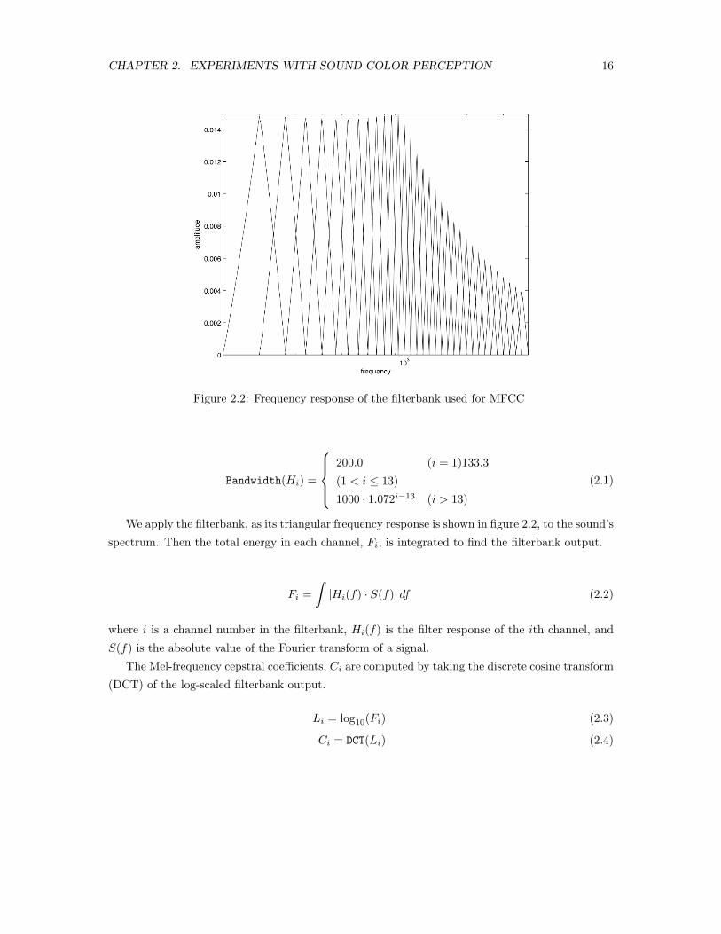
Figure 2.2: Frequency response of the filterbank used for MFCC
Bandwidth(Hi) =
200.0 (i = 1)133.3
(1 < i ≤ 13)
1000 · 1.072i−13 (i > 13)
(2.1)
We apply the filterbank, as its triangular frequency response is shown in figure 2.2, to the sound’s
spectrum. Then the total energy in each channel, Fi, is integrated to find the filterbank output.
Fi =∫|Hi(f) · S(f)| df (2.2)
where i is a channel number in the filterbank, Hi(f) is the filter response of the ith channel, and
S(f) is the absolute value of the Fourier transform of a signal.
The Mel-frequency cepstral coefficients, Ci are computed by taking the discrete cosine transform
(DCT) of the log-scaled filterbank output.
Li = log10(Fi) (2.3)
Ci = DCT(Li) (2.4)

CHAPTER 2. EXPERIMENTS WITH SOUND COLOR PERCEPTION 17
The lower 13 coefficients from C0 to C12, are considered as an MFCC vector, which represents
spectral shape.
2.2.2 Sound Synthesis
The sound synthesis takes two stages: (1) the spectral envelope is created by the pseudo-inverse
transform of MFCC, and (2) an additive synthesis of sinusoids is operated using the spectral envelope
generated earlier.
Pseudo-Inversion of MFCC
MFCC is a lossy transform from a spectrum, therefore in a strict sense, its inversion is not possible.
In this section, the pseudo-inversion of MFCC, the way to generate a smooth spectral shape from
a given set of MFCC is described.
The generation of spectral envelope uses a given array of MFCC Ci, which is an array of the
13 coefficients. The reconstruction of the spectral shape from the MFCC starts with the inverse
discrete cosine transform (IDCT) and amplitude scaling.
Li = IDCT(Ci) (2.5)
Fi = 10Li . (2.6)
In this pseudo-inversion, the reconstructed filterbank output Fi is considered to represent the
value of the reconstructed spectrum S(f) at the center frequency of each filter bank,
S(fi) = Fi (2.7)
where fi is the center frequency of the ith auditory filter. Therefore, in order to obtain the re-
construction of the entire spectrum, S(f), I linearly interpolate the values between the center
frequencies S(fi).
Additive Synthesis
The smooth spectral shape is applied to a harmonic series. A slight amount of vibrato is added to
give some coherence in the resultant sound.
The voice-like stimuli used in this study are synthesized using additive synthesis of frequency-
modulated sinusoids. A harmonic series is prepared, and the level of each harmonic is weighted
based on the desired smooth spectral shape. The pitch, or fundamental frequency f0, is set to

CHAPTER 2. EXPERIMENTS WITH SOUND COLOR PERCEPTION 18
200 Hz, with the frequency of the vibrato v0 set to 4 Hz, and the amplitude of the modulation V
set to 0.02.
Using the reconstructed spectral shape S(f), the additive synthesis of the sinusoid is done as
follows:
s =∑n
S(n · f0) · sin(2πnf0t+ V (1− cos 2πnv0t)) (2.8)
where n specifies the nth harmonic of the harmonic series. The duration of the resulting sound s
is 0.75 second. For the first 30 millisecond of the sound, its amplitude is linearly fading in, and
for the last 30 millisecond of the sound, its amplitude is linearly fading out. All the stimuli are
then scaled with a same scaling coefficient. The specific loudness [Zwicker and Fastl1999] of all the
stimuli showed very small variance, and was considered to be fairly comparable within the stimuli
set.
2.3 Experiment 1: Single-Dimension Sound Color Percep-
tion
2.3.1 Scope
This experiment considers the linear relationship between the perception of sound color and each
coefficient from MFCC, i.e. a single function from the orthogonal set of spectral shape functions.
When the sound synthesis is done in a way that one coefficient from MFCC changes gradually in a
linear manner while the other coefficients are kept constant, the spectral shape of the resulting sound
holds a similar overall shape, but the humps of the shape change their amplitudes exponentially. The
primary question is; “Does the perception of sound color change gradually, in a linear manner, in
good agreement with MFCC?” All of 12 coefficients from MFCC are tested based on this framework.
2.3.2 Method
Participants
Twenty-five normal-hearing participants–graduate students and faculty members from the Center
for Computer Research in Music and Acoustics at Stanford University–volunteered for the exper-
iment. All of them were experienced musicians and/or audio engineers with various degrees of
training.

CHAPTER 2. EXPERIMENTS WITH SOUND COLOR PERCEPTION 19
Figure 2.3: Spectral envelopes generated by varying a single Mel-cepstrum coefficient
Stimuli
Twelve sets of synthesized sounds were prepared. The set n is associated with the MFCC coefficient
Cn—the stimuli set 1 consists of the stimuli with C1 varied, and the stimuli set 2 consists of the
stimuli with C2 varied, and so on. While Cn is varied from zero to one with five levels, i.e.
Cn = 0, 0.25, 0.5, 0.75, 1.0, the other coefficients are kept constant, i.e. C0 = 1 and all other
coefficients are set to zero.
For example, the stimuli set 4 consists of five stimuli based on the following parameter arrange-
ment:
C = [1, 0, 0, 0, C4, 0, ..., 0] (2.9)
where C4 is varied with five levels:
C4 = [0, 0.25, 0.5, 0.75, 1.0]. (2.10)
The figure 2.3 illustrates the idea of varying a single coefficient of MFCC (which is C6 in the
figure), and a resulting set of the spectral envelopes.
Procedure
There were twelve sections in the experiment, one section for each of the twelve sets of stimuli.
Each section consisted of a practice phase and an experimental phase.
The task of the participants was to listen to the sounds, played in sequence with a short interven-
ing silence and to rate the perceived timbre dissimilarity of the presented pair. They entered their
perceived dissimilarity using a 0 to 10 scale, with 0 indicating that the two sounds in the presented

CHAPTER 2. EXPERIMENTS WITH SOUND COLOR PERCEPTION 20
pair were identical, and 10 indicating that they were the most different within the section.
The participants pressed the “Play” button of the experiment GUI using a slider. In order to
facilitate the judgment, the pair having maximal texture difference in the section (i.e., the pair
of stimuli with the lowest and highest, Cn = 0 and Cn = 1, is assumed to have a perceived
dissimilarity of 10) was presented as a reference pair throughout the practice and experimental
phases. Participants were allowed to listen to the testing pair and the reference pair as many times
as they want, but were advised not to repeat too many times, before making their final decision on
scaling, and proceeding to the next pair.
In the practice phase, five sample pairs were presented for rating. In the experimental phase,
twenty-five pairs per section (all the possible pairs from five stimuli) were presented in a random
order. The order of presenting the sections was randomized as well.
Figure 2.4 provides the screen snapshot of the graphical interface for the experiment. The
following instruction was given to the participants before starting an experiment.
Instruction for the experiment:
This experiment is divided into 12 sections. Each section presents 10 practice trials
followed by 25 experiment trials. Every trial presents a pair of short sounds. Your task
is to rate the timbre dissimilarity of the paired sounds using a numerical scale from 0
to 10 using the slider on the computer screen, where 0 represents the two sounds being
identical, and 10 represents the sounds being most different within the section.
When you are ready to hear a trial, press “Play” button and listen to the paired sounds.
Using the slider, rate the perceived difference between the sounds. Press Reference
button in order to listen to the most different pair of the current section. You may
rehear the sounds by pressing the “Play” or “Reference” button, and you may re-adjust
your rating. When you are satisfied with your rating submit the result by pressing the
“Next” button, and proceed to the next trial.
Each section consists of a different set of sound stimuli. The practice trials present the
full range of timbral difference within a section. Please try to use the full scale of 0
to 10 in rating your practice trials and then be consistent with this scale during the
following experiment trials. In deciding the dissimilarity of timbre quality, try to ignore
any differences in perceived loudness or pitch of the paired sounds.
When rating the dissimilarity, please give your response in approximate increments of
0.5 scale (e.g. 5.0 , 5.5, or at the middle of the grid at finest–but not 6.43.) Use the
grids above the slider as a general guide rather than for precise adjustment. Please feel
free to take a brief break during the section as needed. Taking longer breaks between

CHAPTER 2. EXPERIMENTS WITH SOUND COLOR PERCEPTION 21
Figure 2.4: Graphical user interface for the experiment
sections is highly recommended: pause, stretch, relax, and resume the experiment.
2.3.3 Analysis 1. Linear Regression
The dissimilarity judgments were analyzed using simple linear regression (also known as least-
squares estimation) [Mendenhall and Sinich1995], with absolute Cn differences as the independent
variable, and their reported perceived dissimilarities as the dependent variable. The coefficient of
determination (R2, R2, or R-squared) represents the goodness of fit in the linear regression analysis.
Because it is anticipated that every person’s perception is individual, I first applied individual
linear regression for each section and each participant. The R2 values of one section from all the
participants were then averaged to find the mean degree of fit (mean R2) of each section. The
mean R2 among participants is used to judge the linear relationship between the Cn distance and
perceived dissimilarity.
The mean R2 and the corresponding confidence interval are plotted in the figure 2.5. The mean
R2 of the entire responses were 85 %, with the confidence intervals for all the sections overlapped.
This means that all of the coefficients, from C1 to C12, have a linear correlation to the perception of
sound color with the statistically equivalent degree of fit, when a coefficient is tested independently
from the other coefficients.

CHAPTER 2. EXPERIMENTS WITH SOUND COLOR PERCEPTION 22
Figure 2.5: Coefficients of determination (R2) from regression analysis of the single-dimensionalsound color experiment
2.3.4 Analysis 2. Equivalence Test in Pairwise Comparison
An issue of this experiment is that an experiment session took about 45 minutes to two hours,
depending on the participant. Reducing the number of stimulus pairs to be tested is desirable,
to avoid the participants’ fatigue and to encourage the participation in the experiment. During
this single color experiment, I tested all the possible pairs from a session’s five stimuli. This
arrangement provided 25 pairs, with 10 duplicating pairs with an alternate order (the pairs of AB
and BA). The equivalence testing [Rogers et al.1993] was operated to test the symmetry in the
subjective judgments (i.e. testing whether the perceived distances for AB and BA are statistically
equivalent or not), with the hope that if the judgments are symmetrical, I do not have to test all
the possible pairs but about the half of the pairs.
First I ran two linear regression analyses: one using only AB responses, and the other one using
only BA responses. I calculated the mean R2 for AB responses regression among the participants for
each section, and the other mean R2, for BA responses regression. The two mean R2 were compared
for equivalence. According to Rogers’ method, the confidence interval test was operated with the a
priori defined delta (the minimum difference between two groups to be considered nonequivalent)
set to 5 %. The equivalence interval fell into the 5 % minimum difference range, therefore the
regression analyses based on AB responses and BA responses were determined to be symmetrical.

CHAPTER 2. EXPERIMENTS WITH SOUND COLOR PERCEPTION 23
From this result, I consider that the subjective judgments on the alternate stimuli presentation
order (stimuli pair of AB and BA) are equivalent.
2.3.5 Analysis 3. Spectral Centroid Assessment
Another interest is the correlation with the spectral centroid. It is said that the spectral centroid has
a strong correlation with the perceived brightness of sound [Schubert and Wolfe2006]. I calculated
the spectral centroid for each of the stimuli used in the experiment, as shown in figure 2.6. The
MFCC-based stimuli and their spectral centroids are linearly correlated. The C1 stimuli had lower
centroids while C1 increases from 0 to 1, and the C2 stimuli had higher centroids while C2 increases,
but with smaller coefficient (less slope), and so on: in summary, lower MFCC coefficients have
stronger correlation to the spectral centroid, and the correlation is negative in case of odd-numbered
MFCC dimensions (spectral centroid decreases while Cn increases where n is an odd number), and
positive in case of even-numbered MFCC dimension (spectral centroid increases while Cn increases,
where n is an even number).
This is not a surprising effect, having seen the trend in spectral envelopes generated for this
experiment as shown in figure 2.3. Looking at the spectral envelopes generated by varying C1,
there is a hump around the low-frequency range, which corresponds to the cosine wave at ω = 0,
and there is a dip around the Nyquist frequency, which corresponds to ω = π/2. As C1 increases,
the magnitude of the hump becomes higher. The concentrated energy around the low-frequency
region corresponds to the lower spectral centroids while increasing the value of C1. Now, if we
observe the spectral envelopes generated by varying C2, there are two humps at the DC and the
Nyquist frequency, corresponding to ω = 0 and ω = π. Having another hump at the Nyquist
frequency makes the spectral centroid higher; whereas increasing the value of C2 increases the
spectral centroid.
The same trends are conserved for odd- and even-numbered MFCC coefficients. However, the
higher the dimension of the MFCC, the more energy is sparsely distributed over the spectrum,
which makes the coefficient of the linear relationship between MFCC and spectral centroid smaller
(i.e. the slope of the line which plots MFCC and spectral centroid becomes more shallow, when n
is higher).
The above-mentioned points are all dependent on the specific implementation of MFCC, and the
pseudo-inversion of MFCC, used in this experiment. Depending on how the MFCC and its inversion
are implemented, it could have different kinds of relationships to the spectral centroid. However,
there was a trend in the spectral centroids in my MFCC-based stimuli set, and it coincides well
with the reported experiments about the correlation between timbre perception and the spectral
centroid.

CHAPTER 2. EXPERIMENTS WITH SOUND COLOR PERCEPTION 24
Figure 2.6: Spectral centroid of the stimuli used for the single-dimensional sound color experiment
2.3.6 Discussion
In this experiment, it is shown that every orthogonal basis from MFCC is linearly correlated to
human perception of sound color at about 85% degree of fit. The subjective responses to the
pairs of alternate order (perceived dissimilarity between AB or BA) are symmetric. There is a
linear relationship between the Cn values and the spectral centroids of the synthesized sounds
using them, which provides an agreement between the results from this experiment and the other
experiments on spectral centroid and timbre perception.
2.4 Experiment 2: Two-dimensional Sound Color Percep-
tion
2.4.1 Scope
In this experiment, the perception of the two-dimensional sound color space is tested. The stimuli
set was synthesized by varying two coefficients from MFCC array, say Cn1 and Cn2, to form a two-
dimensional subspace. The subjective response to the stimuli set is tested based on the Euclidean
space hypothesis: if each coefficient functions as an orthogonal basis to estimate the sound color

CHAPTER 2. EXPERIMENTS WITH SOUND COLOR PERCEPTION 25
perception. Since it is difficult to test all the 144 two-dimensional subspaces, five two-dimensional
subspaces were chosen to be tested.
2.4.2 Method
Participants
Nineteen normal-hearing participants, who were audio engineers, administrative staff, visiting com-
posers, and artists from Banff Centre, Alberta, Canada, volunteered for the experiment. All of
them had a strong interest in music, and some of them received professional training in music and
audio engineering.
Stimuli
Five sets of synthesized sounds were prepared. They are associated with the five different kinds
of two-dimensional subspaces. The five subspaces are made by varying [C1, C3], [C3, C4], [C3, C6],
[C3, C12], and [C11, C12], respectively. For each set, the coefficients in question are independently
varied over four levels (Cn = 0, 0.25, 0.5, 0.75), the other coefficients are kept constant, i.e. C0 = 1
and all other coefficients are set to zero. By varying two coefficients independently, over four levels,
each set has 16 synthesized sounds.
For example, the first set made of the subspace [C1, C3] consists of the 16 sounds based on the
following parameter arrangement:
C = [1, C1, 0, C3, 0, ..., 0] (2.11)
where C1 and C3 are varied over four levels, creating a grid with two variables.
The subspaces were chosen with the intention to test the spaces made out of: non-adjacent low
to middle coefficients ( [C1, C3], and [C3, C6]); two adjacent low coefficients ([C3, C4]); low and high
coefficients ([C3, C12]); and two adjacent high coefficients ([C11, C12]).
The figure 2.7 shows an example of the generated spectral envelopes for this experiment.
Procedure
There are 16 stimuli sounds per one subspace. All the possible combination of pairwise presentation
makes 256 pairs. It is difficult to test all of these pairs because of the limited time. Reducing the
number of test pairs can also reduce exhaustion of the participants.
From the first experiment, in which the perceived distances between sound A and B are mea-
sured, the perceived distances, AB and BA are statistically equivalent. Therefore, in this experi-
ment, I tested only one of two possible directions of a pairwise presentation of two sounds. Within
CHAPTER 2. EXPERIMENTS WITH SOUND COLOR PERCEPTION 26
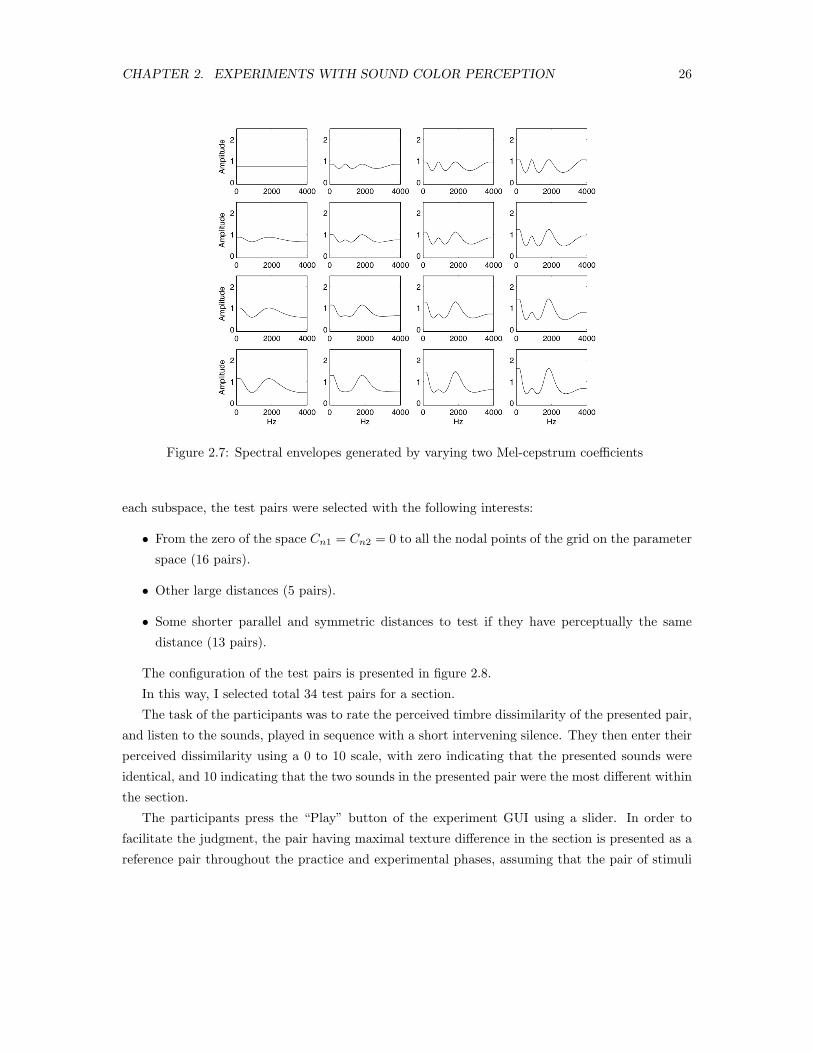
Figure 2.7: Spectral envelopes generated by varying two Mel-cepstrum coefficients
each subspace, the test pairs were selected with the following interests:
• From the zero of the space Cn1 = Cn2 = 0 to all the nodal points of the grid on the parameter
space (16 pairs).
• Other large distances (5 pairs).
• Some shorter parallel and symmetric distances to test if they have perceptually the same
distance (13 pairs).
The configuration of the test pairs is presented in figure 2.8.
In this way, I selected total 34 test pairs for a section.
The task of the participants was to rate the perceived timbre dissimilarity of the presented pair,
and listen to the sounds, played in sequence with a short intervening silence. They then enter their
perceived dissimilarity using a 0 to 10 scale, with zero indicating that the presented sounds were
identical, and 10 indicating that the two sounds in the presented pair were the most different within
the section.
The participants press the “Play” button of the experiment GUI using a slider. In order to
facilitate the judgment, the pair having maximal texture difference in the section is presented as a
reference pair throughout the practice and experimental phases, assuming that the pair of stimuli

CHAPTER 2. EXPERIMENTS WITH SOUND COLOR PERCEPTION 27
Figure 2.8: Selection of the test pairs for the two-dimensional sound color experiment
with the lowest and highest, Cn1 = Cn2 = 0 and Cn1 = Cn2 = 0.75, would have a perceived
dissimilarity of 10 within the stimuli set. Participants were allowed to listen to the testing pair and
the reference pair as many times as they wanted, but were advised not to repeat too many times,
before making their final decision on scaling, and proceeding to the next pair.
In the practice phase, five sample pairs were presented for rating. In the experimental phase,
34 pairs per section were presented in a random order. The order of presenting the sections was
randomized as well.
The figure 2.4 provides the screen snapshot of the graphical interface for the experiment. The
following instruction was given to the participants before starting an experiment.
Instruction for the experiment:
This experiment is divided into 5 sections. Each section presents 5 practice trials fol-
lowed by 34 experiment trials. Every trial presents a pair of short sounds. Your task
is to rate the timbre dissimilarity of the paired sounds using a numerical scale from 0
to 10 using the slider on the computer screen, where 0 represents the two sounds being
identical, and 10 represents the sounds being most different within the section.
When you are ready to hear a trial, press “Play” button and listen to the paired sounds.
Using the slider, rate the perceived difference between the sounds. Press “Reference”
button in order to listen to the most different pair of the current section. You may
rehear the sounds by pressing the “Play” or “Reference” button, and you may re-adjust
your rating. When you are satisfied with your rating submit the result by pressing the
“Next” button, and proceed to the next trial.
Each section consists of a different set of sound stimuli. The practice trials present the
full range of timbral difference within a section. Please try to use the full scale of 0 to 10

CHAPTER 2. EXPERIMENTS WITH SOUND COLOR PERCEPTION 28
in rating your practice trials and then be consistent with this scale during the following
experiment trials.
When rating the dissimilarity, please give your response in approximate increments of
0.5 scale. Use the grids above the slider as a general guide rather than for precise
adjustment.
Please feel free to take a brief break during the section as needed. Taking longer breaks
between sections is highly recommended: pause, stretch, relax, and resume the experi-
ment.
2.4.3 Multiple Regression Analysis
The dissimilarity judgments were analyzed using multiple linear regression. The orthogonality of the
two-dimensional subspaces was tested with a Euclidean distance model: The independent variable
is the Euclidean distance of MFCC between the paired stimuli, and the dependent variable is the
subjective dissimilarity rating.
d2 = ax2 + by2 (2.12)
Where d is the perceptual distance that subjects reported in the experiment, x is the difference of
Cn1, and y is the difference of Cn2 between the paired stimuli. The coefficient of determination, R2
represents the goodness of fit in the linear regression analysis.
Individual linear regression for each section and each participant is first applied. The R2 values
of one section from all the participants were then averaged to find the mean degree of fit (mean R2)
of each section. The mean R2 among participants is used to observe if the perceived dissimilarity
reflects the Euclidean space model.
The mean R2 and the corresponding confidence interval are plotted in figure 2.9. The mean
R2 of all responses was 74% with the confidence intervals for all the sections overlapped. This
means that all of the five subspaces demonstrate a similar degree of fit to a Euclidean model of
two-dimensional sound color perception regardless of the various choice of the coordinates from
MFCC space.
The figure 2.10 shows the regression coefficients (i.e. a and b from the equation 2.12) for each
of the two variables from the regression analysis for all five sections. The regression coefficients
were consistently higher for a lower one of the two MFCC variables, meaning lower Mel-cepstrum
coefficients are perceptually more significant. The stronger association between lower Mel-cepstrum
coefficients and spectral centroid may explain this result on regression coefficients.

CHAPTER 2. EXPERIMENTS WITH SOUND COLOR PERCEPTION 29
Figure 2.9: Coefficient of determination (R2) from regression analysis of the two-dimensional soundcolor experiment. Sections 1–5 represent the tests on subspaces [C1, C3], [C3, C4], [C3, C6], [C3, C12],and [C11, C12], respectively.

CHAPTER 2. EXPERIMENTS WITH SOUND COLOR PERCEPTION 30
Figure 2.10: Regression coefficients from regression analysis of the two-dimensional sound colorexperiment. The first two points on the left represent the regression coefficient for each dimensionof the [C1, C3] subspace, followed by regression coefficients for the subspaces of [C3, C4] [C3, C6],[C3, C12], and [C11, C12].

CHAPTER 2. EXPERIMENTS WITH SOUND COLOR PERCEPTION 31
2.4.4 Discussion
In this experiment I tested the association between the perceptual sound color space and the
two dimensional sound color space designed by MFCC. The Euclidean distance model explains
the perceived sound color space perception at 74% degree of fit on average. The five different
arrangements of 2D subspaces were selected, and all the arrangements showed a similar degree
of fit to the Euclidean model. Examining the regression coefficients demonstrated that the lower
MFCC coefficients had the stronger effect in perceived sound color space.
2.5 Chapter Summary and Future Work
In this chapter I discussed the perception of sound color. Based on desirable properties for a sound
color model (linearity, orthogonality, and multidimensionality), I proposed Mel-frequency cepstral
coefficients (MFCC) as a metric and reported two quantitative experiments on their relation to hu-
man perception.The quantitative data from the experiment exhibit the linear relationship between
the subjective perception of complex tones and the proposed metric for spectral envelope.
The first experiment tested the linear mapping between the human perception of sound color
and each of all twelve Mel-cepstrum coefficients. Each Mel-cepstrum coefficient showed a linear
relationship to the subjective judgment at the statistically equivalent level to any other coefficient.
On average, the MFCC explains 85% of the perceived dissimilarity in sound color when a single
coefficient from MFCC is varied in an isolated manner from the other coefficients.
In the second experiment I varied two Mel-cepstrum coefficients in order to form a two-dimensional
(2D) sound color subspace and tested its perceptual relevance. A total of five subspaces were tested,
and all five cases exhibited the linear relationship to the perceptual responses at a statistically equiv-
alent level. The subjective dissimilarity rating showed the correlation of 74% on average to the
Euclidean distance between the Mel-cepstrum coefficients of the tested stimulus pair. This means
that a two-dimensional MFCC-based sound color space matches perceptual sound color space. In
addition, the observation of regression coefficients demonstrated that lower-order Mel-cepstrum
coefficients influence human perception more strongly.
Both the one- and two-dimensional experiments are consistent with the MFCC model providing a
linear and orthogonal coordinate space for human perception of sound color. Such a representation
can be useful not only in analyzing audio signals, but also in controlling timbre in synthesized
sounds.
I have only explored the MFCC model experimentally at low dimensionality. Much work re-
mains to be done in understanding how MFCC variation across the entire 12 dimensions might
relate to human sound perception. An interesting approach is currently being taken by Horner,

CHAPTER 2. EXPERIMENTS WITH SOUND COLOR PERCEPTION 32
Beauchamp, and So who are taking their previous experimental data on timbre morphing of instru-
mental sounds [Horner et al.2006] and re-analyzing it using MFCC (in preparation). Their approach
using instrumental sounds will provide a good complement to the approach taken here.

Chapter 3
Explorations of Density
3.1 Introduction
In this chapter I investigate the perception of density and introduce a prospective model of density
perception. Density is, as defined in chapter 1, the fluctuation of instantaneous intensity of a
particular sound, both in terms of rapidity of change and degree of differentiation between sequential
instantaneous intensities. Density represents the fine-scale temporal attribute which complements
the spectral description (sound color). With the same motivations as the quantitative model for
sound color perception, I aim to establish a quantitative model for density perception, which is
simple, compact, and yet descriptive.1
In establishing the model of density, many research works are conceptually relevant and in-
spiring, such as texture mapping in computer graphics [Heckbert1986], tactile and multi-sensory
perception of texture [Lederman and Klatzky2004], wavelet-based texture synthesis
[Saint-Arnaud and Popat1998, Dubnov et al.2002, Athineos and Ellis2003], and the concept of gran-
ularity in room acoustics [Huang and Abel2007]. These works observe the small-scaled fluctuation
of a matter, such as visual color, structure of surface gratings or fabric weaves, and amplitude of a
sound’s waveform. Such small-scaled fluctuations would produce a particular sensual quality, which
is often denoted as granularity, texture, and coarseness; this is the quality which I use the word
density to describe. In the above listed works in the audio domain researchers explored the analysis
or synthesis of density as physical characteristics, but there has not been a study on the perceived1The density experiments are the product of a joint project with Patty Huang and Jonathan Abel. In response to
their preliminary report based on an informal listening test [Huang and Abel2007], I proposed to run a formal psy-choacoustic experiment, and we ultimately operated three density experiments together. In preparation, I contributedthe experiment design and setup, they contributed the stimuli synthesis, and we jointly carried out the data collectionand analysis. These experiments were previously reported at conferences [Terasawa et al.2008, Huang et al.2008].
33

CHAPTER 3. EXPLORATIONS OF DENSITY 34
quality of density. This chapter is dedicated to the experimental study of the perception of density
and to establishing a quantitative model of density perception.
In the ideal density model, I seek the following characteristics: The density model should be able
to analyze the density, or at least the stochastic quality2 of a sound; the model should quantitatively
predict the human perception of density with a linear mapping; and the model should robustly
represent the perceived density of the sounds regardless of their arbitrary sound color.
The notion of density may not be familiar, but this term has been used in music theory and
room acoustics. In music theory, density has number of meanings including the number of sounds
happening concurrently, and in room acoustics, echo density means the number of echoes per unit
time. In music theory 3, composer and music theorist Wallace Berry offers the following definition
of density in his book Structural Functions in Music [Berry1976]:
Density is defined as that textural parameter, quantitative and measurable, conditioned
by the number of simultaneous or concurrent components and by the extent of vertical
‘space’ encompassing them.
To summarize, this definition is about how many sounds there are and if they are resolved or fused.
The same amount of musical components will sound sparse or condensed, depending on the vertical
space (i.e. pitch range on the musical score) being more or less. When the notion of density appears
in room acoustics and artificial reverberation, the echo density is defined as the number of echoes
found in an impulse response of a space without considering the spectral aspects [Schroeder1962]:
The number of echoes per second at the output of the reverberator for a single pulse at
the input.
The stage of early reflections of the room reverberation shows fewer, but discernible, echoes, and
the stage of late reverberation shows more echoes fused into each other. Therefore the notion of
echo density is useful to characterize the transitory stages of the reverberation.
Although these two definitions come from divergent disciplines, they share a common perspective
in which density represents a physical quantity per unit time. However, this work aims for a metric
which can directly estimate the perceptual quality based on physical characteristics. Therefore,2The scope of density is larger than stochastic elements of sound, and it could cover, for example, periodic
fluctuations of instantaneous intensity. However, in this thesis, assuming that periodic elements are perceived smooth,I focus on the problem of representing irregular and aperiodic temporal qualities.
3Another definition of density [Rowell1983] is “Thin/dense refers to the number of simultaneous sounds and theirrelative distribution over the pitch spectrum from low to high. Musical density ranges from a solo line to texturesof more than fifty parts, as in Penderecki’s Threnody for the Victims of Hiroshima, but most musical textures areclose to the thin end of the scale.” However, this term is used in a variety of context according to Griffith’s definitionof density from The Oxford Companion to Music (Revised edition, 2002): “An informal measure of polyphoniccomplexity, chord content, or general sound, chiefly used of 20th-century music where a more precise vocabularydoes not exist. One may thus speak of dense textures, dense harmonies, etc.”

CHAPTER 3. EXPLORATIONS OF DENSITY 35
I would like to establish a model which can transform a physical description into a perceptually
meaningful metric of density.
Surprisingly, room reverberation research methodologies proved to be conceptually most relevant
to accomplishing this task. In this discipline researchers investigate the characteristics of an impulse
response in its irregular and aperiodic sequence of echoes. Such characteristics, of course, cannot
be detected by a spectral analysis because such a temporal quality remains invisible behind a blur
of broad-band responses. In order to solve this problem, room-acoustics researchers have been
observing the rapid fluctuation of sound intensity in the time domain so that they can describe the
temporal characteristics of the reverberation impulse response with quantitative representations.
Although the sounds in the research subject come from room reverberation impulse responses,
the temporal characteristics of the sounds–the irregular and aperiodic sequence of impulses–are no
different from the stochastic portions of musical, spoken, and environmental sounds (as opposed to
their harmonic elements), which can be represented as a series of irregularly occurring impulses with
noise-like qualities. For that reason, the knowledge acquired by studying the room reverberation can
be applicable to other types of sounds. Therefore, in this study I decided to study the perception
of reverberation echo density in order to understand the perception of density.
The current problem with echo density (or absolute echo density, AED) is that counting the
actual number of echoes is easily affected by noise bandwidths and is not capable of describing the
perceived quality across different bandwidths. Abel and Huang proposed normalized echo density
(NED) to overcome this obstacle. This measure estimates the noise quality by observing how much
the noise mixture resembles Gaussian distribution and is insensitive to the equalization.
In addition to this metric, NED, there have been a few methods proposed in terms of the
“Gaussian-ness” of the impulse response in order to model the transition from early reflections to
late reverberation [Stewart and Sandler2007, Defrance and Polack2008]. While these other meth-
ods observe the similarity to the Gaussian noise by Kurtosis analysis, NED searches the outliers
from Gaussian distribution upon the assumption that the sound of interest is reverberation noise.
Although NED differs from Kurtosis analysis, these two approaches share the idea of observing
the proximity to the statistical property of Gaussian mixture noise. Abel and Huang also reported
that both the NED- and Kurtosis-based metrics demonstrate similar results in analyzing a room
reverberation impulse response [Abel and Huang2006].
However, the relevance of the statistical property of the room reverberation impulse response,
and the perceived noise quality, was not discussed until Huang and Abel’s next report
[Huang and Abel2007]. In this paper they reported that normalized echo density well predicts
human perception of the noise quality regardless its bandwidth, although by informal listening.
Considering these reports, NED seems to have good potential to function as a perceptual density
model–directly addressing the perceptual density while being unaffected by the coloring of the

CHAPTER 3. EXPLORATIONS OF DENSITY 36
sound. Therefore, in this chapter I employ NED as a hypothetical model for perceptual density, and
examine the relationship between the estimated density of NED and the quantitative measurement
of the perceived density through formal psychoacoustic experiments.
In search of the perceptually relevant metric of density, currently there has been no other
comparable method to NED. Because the metric for the reverberation mixing time is still evolving
in the research field, I have to admit that there may or may not be some other methods in the
future which could be suitable for perceptual density modeling. However, I foresee two merits in
operating the psychoacoustic experiment of NED: At most, the experiment result can be equally
applicable to Kurtosis-based methods, because NED functions similarly to Kurtosis-based analysis
for aperiodic noise-like sounds. At least we have the data on perception of noise-like sounds which
can be re-analyzed by any other method when we find a better candidate for a density model.
The three experiments described in this chapter aim to investigate perceptual sound density.
In these experiments we used artificially synthesized noise-like stimuli which have consistent sound
density within a stimulus. The synthesized noise stimuli enabled us to conduct reliably quantitative
measurements.
The first experiment aims to test if normalized echo density is a metric which directly represents
the perceived density. It takes a similar style to the sound color experiment: We presented stimuli
with various normalized echo densities and bandwidths in pairs. After acquiring the subjective
dissimilarity judgments we tested the relationship between the perceived density dissimilarity and
the difference of normalized echo density.
The second experiment uses a “grouping” framework to investigate the consistency across band-
widths. We asked the participants to mark breakpoints in a sequence of noises with gradually
changing echo densities. This experiment aims to determine whether the grouping behavior is con-
sistent across different bandwidths. For example, if we listen to a noise with a narrow bandwidth
and another noise with a higher bandwidth the questions are 1) if we show a consistent judgment
of perceived sound density across bandwidths and 2) if that judgment can be well explained using
normalized echo density.
The third experiment explores the same concern using a “matching” framework. In this exper-
iment, the participants matched the perceived sound density of a noise with one bandwidth, and
another with another bandwidth. With this experiment, we tested whether the density perception
estimated by NED is constant across bandwidths.
In the next sections, the algorithm of the normalized echo density and the noise synthesis is
described, followed by sections which describe the experimental procedures and results.

CHAPTER 3. EXPLORATIONS OF DENSITY 37
3.2 Normalized Echo Density
Over a sliding window of a reverberation impulse response, the normalized echo density profile η(t)
is the fraction of impulse response taps which lie outside the window standard deviation, normalized
to that expected for Gaussian noise:
η(t) =1/erfc(1/
√2)
2β + 1
t+β∑τ=t−β
{|h(τ)| > σ}, (3.1)
where h(t) is the reverberation impulse response (assumed to be zero mean), 2β + 1 is the
window length in samples, σ is the window standard deviation,
σ =
12β + 1
t+β∑τ=t−β
h2(τ)
12
, (3.2)
{·} is the indicator function, returning one when its argument is true and zero otherwise, and
erfc(1/√
2) .= 0.3173 is the expected fraction of samples lying outside a standard deviation from
the mean for a Gaussian distribution [Abel and Huang2006].
The normalized echo density profile (NEDP) is more generally computed using a positive weight-
ing function w(t) so as to de-emphasize the impulse response taps at the sliding window edges:
η(t) =1
erfc(1/√
2)
t+β∑τ=t−β
w(τ){|h(τ)| > σ} (3.3)
with
σ =
t+β∑τ=t−β
w(τ)h2(τ)
12
(3.4)
and where w(t) is normalized to have unit sum∑τ w(τ) = 1.
Figure 3.1 shows the normalized echo density profile of a measured room impulse response using
a 20 ms Hanning window. NED values are near zero during the early reflection portion of the
reverberation, indicating a low echo density. The NED value increases over time to a value near
one, suggesting Gaussian-like statistics, where it remains for the duration of the impulse response.
As described in [Abel and Huang2006], what sets one NED profile apart from another is the rate
of increase and the time at which a value near one is first attained, indicating the start of the late
field.
As developed in [Huang and Abel2007], the normalized echo density η can be related to the
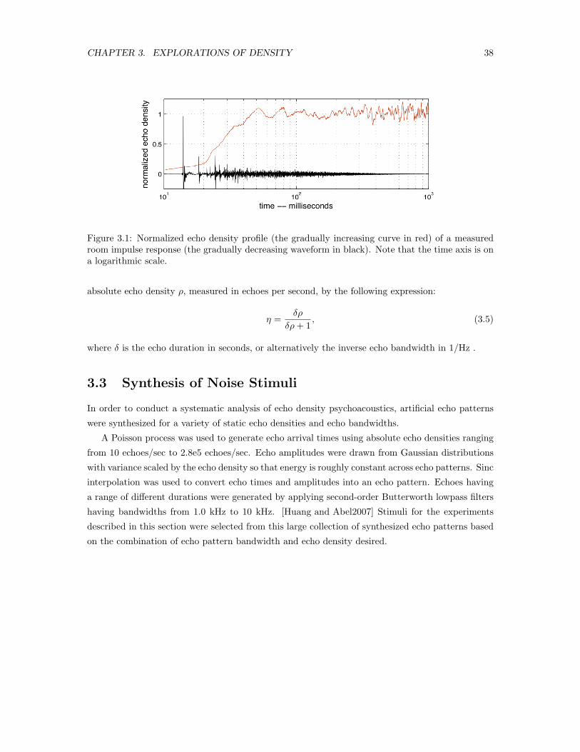
CHAPTER 3. EXPLORATIONS OF DENSITY 38
Figure 3.1: Normalized echo density profile (the gradually increasing curve in red) of a measuredroom impulse response (the gradually decreasing waveform in black). Note that the time axis is ona logarithmic scale.
absolute echo density ρ, measured in echoes per second, by the following expression:
η =δρ
δρ+ 1, (3.5)
where δ is the echo duration in seconds, or alternatively the inverse echo bandwidth in 1/Hz .
3.3 Synthesis of Noise Stimuli
In order to conduct a systematic analysis of echo density psychoacoustics, artificial echo patterns
were synthesized for a variety of static echo densities and echo bandwidths.
A Poisson process was used to generate echo arrival times using absolute echo densities ranging
from 10 echoes/sec to 2.8e5 echoes/sec. Echo amplitudes were drawn from Gaussian distributions
with variance scaled by the echo density so that energy is roughly constant across echo patterns. Sinc
interpolation was used to convert echo times and amplitudes into an echo pattern. Echoes having
a range of different durations were generated by applying second-order Butterworth lowpass filters
having bandwidths from 1.0 kHz to 10 kHz. [Huang and Abel2007] Stimuli for the experiments
described in this section were selected from this large collection of synthesized echo patterns based
on the combination of echo pattern bandwidth and echo density desired.

CHAPTER 3. EXPLORATIONS OF DENSITY 39
3.4 Experiment 3: Dissimilarity of Perceptual Density
3.4.1 Scope
In this experiment, we investigated the relationship between NED and perception of echo patterns
with static echo densities. Our primary interests are (1) whether the density descriptions (NED,
AED, and log of AED) relate in a simple way to perceived density dissimilarity, and (2) if those
relationships are consistent across bandwidths (i.e., echo durations).
3.4.2 Method
Participants
Twenty-five normal-hearing participants, graduate students and faculty members from Center for
Computer Research in Music and Acoustics at Stanford University, volunteered for the experiment.
All of them were experienced musicians and/or audio engineers with various degrees of training.
Stimuli
Three sets of echo patterns having five different static echo densities (NED = 0.13, 0.24, 0.57, 0.74,
0.90) were generated with each set having different echo bandwidths (1 kHz, 2 kHz, and 5 kHz,
corresponding to echo durations of roughly 1.0 ms, 0.5 ms, and 0.2 ms, respectively). The density
of the stimuli was varied so that granularity ranged from sparse to smooth, while the other factors
such as duration, loudness, and bandwidth, were kept constant.
Procedure
There were three sections in the experiment, one section for each of the three sets of the stimuli.
Each section consisted of a practice phase and an experimental phase.
The task of the participants was to listen to the sounds played in sequence with a short in-
tervening silence and to rate the perceived density dissimilarity of the presented pair. They then
entered their perceived dissimilarity using a 0 to 10 scale, with zero indicating that the presented
sounds were identical and 10 indicating that the two sounds in the presented pair were the most
different within the section.
The participants pressed the “Play” button of the experiment GUI using a slider. In order to
facilitate the judgment, the pair having maximal density difference in the section (i.e., the pair of
lowest and highest echo density sequences, defined to have a dissimilarity of 10) was available as a
reference pair throughout the practice and experimental phases. Participants were allowed to listen
to the testing pair and the reference pair as many times as they wanted, but they were advised not

CHAPTER 3. EXPLORATIONS OF DENSITY 40
to repeat too many times before making their final decision on scaling and proceeding to the next
pair.
In the practice phase, five sample pairs were presented for rating. In the experimental phase,
twenty-five pairs per section (all the possible pairs from five stimuli) were presented in a random
order. The order of presenting the sections was randomized as well.
It should be pointed out that the maximally dissimilar pair used as a reference employed different
sequences than those presented for rating. Also, so as to distinguish the ability to discern different
sequences having identical echo densities from the ability to recognize identical sounds, two different
sequences were generated at each echo density, and each pair presented drew one sound from each
generation.
The figure 3.2 provides the screen snapshot of the graphical interface for the experiment. The
following is the instruction given to the participants before starting an experiment.
You will have 4 sections in this experiment. Each section has 5 practice trials followed
by 25 experiment trials. Every trial has a pair of short sounds. Your task is to rate the
timbre dissimilarity of the paired sounds using a numerical scale from 0 to 10 using the
slider on the computer screen, where 0 represents two sounds being identical, and ten
represents the sounds being very different.
At each trial, press Play button and listen to the paired sounds. Using the slider, rate
how different the paired sounds are. You may repeat listening to the sounds by pressing
the play button, and you may re- adjust your rating. Submit the final rating by pressing
“Next” button, and proceed to the next trial. Each section consists of a different group
of sounds to create those pairs. The practice trials project the range of timbral difference
within a section. Please try to use up the full scale of 0 to 10 during the practice, and
be consistent with that during the following experiment trials.
In deciding the dissimilarity of timbre quality, try to ignore any differences which may
be there due to the loudness or the pitch of the paired sounds.
When rating the dissimilarity, please give your response by roughly 0.5 scale (e.g. 5.0 ,
5.5, or at the middle of the grid at finest - but not 6.43.) Use the grids above the slider
as your guidance, but you do not have to precisely adjust to the grid, as long as the
slider position agrees to your perception. Please feel free to take a brief break during
the section as needed. Taking longer breaks between sections is highly recommended:
pause, stretch, relax, and resume the experiment.

CHAPTER 3. EXPLORATIONS OF DENSITY 41
Figure 3.2: Graphical user interface for the dissimilarity test
3.4.3 Analysis
The dissimilarity judgments were analyzed using linear regression (also known as least squares
estimation) [Mendenhall and Sinich1995] with absolute NED differences as the independent variable
and their reported perceived dissimilarities as the dependent variable.
The mean of the coefficient of determination (R2, R2, or R-squared, which represents the good-
ness of fit) among participants is used to judge the linear relationship between the NED distance
and perceived dissimilarity. We first applied individual linear regression for each section and each
participant. The R2 values of one section from all the participants were then averaged to find the
mean degree of fit (mean R2) of each section.
In addition to the NED-based analysis, the same analyses were repeated using distances based
on AED and on log AED, as independent variables. Figure 3.3 shows mean R2 values from the
linear regression analyses based on these three independent variables.
Absolute difference in NED is a good model for perceived density dissimilarity, having a mean
R2 of 93%. The log AED is a reasonable indicator of density dissimilarity, with a mean R2 of 88%.

CHAPTER 3. EXPLORATIONS OF DENSITY 42
Figure 3.3: Mean R2 and 95% confidence intervals of linear regression on perceptual dissimilarityof echo patterns having static echo densities using AED (o), log AED (.), and NED (*) as theindependent variable.
AED, however, fails as a usable model.
3.5 Experiment 4: Density Grouping
3.5.1 Scope
This experiment inherits the framework for the preliminary study described in [Huang and Abel2007].
The basic idea is to understand if there are any commonly perceived anchors in the perception of
gradually changing density, e.g., if there are clear boundaries to divide the density clusters when
the density is changing from smooth to rough, and if so, if the boundaries are common across
bandwidths.
In this experiment, we asked the participants to divide the static echo noises into three groups
and observed the trend in the reported boundaries. Also of interest was whether a boundary point

CHAPTER 3. EXPLORATIONS OF DENSITY 43
in NED is consistent among echo patterns with various bandwidths.
3.5.2 Method
Participants
Nine normal-hearing participants, musicians, recording engineers, and staff from the Department
of Music and Sound at the Banff Centre, volunteered for the experiment.
Stimuli
Four sets of echo patterns having 19 different static echo densities (NED = 0.05, 0.10, 0.15, ...,
0.95) were generated at each of four bandwidths (1 kHz, 2 kHz, 5 kHz, and 10 kHz). The density
of the stimuli was varied so that granularity ranged from sparse to smooth while the other factors
such as duration, loudness, and bandwidth, were kept constant.
Procedure
Buttons allowing the subject to listen to the nineteen static noise patterns were presented in as-
cending NED order. The participants were instructed to listen to the noise patterns as many times
as they wished and in whatever order. They were asked to select two breakpoints, grouping the
noise sequences into three density regions, e.g., rough, medium, and smooth. The sections were
organized by bandwidth, and the order of section presentation was randomized.
The figure 3.4 provides the screen snapshot of the graphical interface for the experiment. The
following are the instructions given to the participants before starting an experiment.
There are 4 sections in this experiment. In each section, you will find a set of numbered
square buttons, two rows of round buttons aligned between the square buttons, “Se-
quence up”, “Sequence down”, and “Next’ buttons. By pressing a square button, you
will hear its associated sound. By pressing the “Sequence up” button, you will hear all
the sounds in sequence, and by pressing the “Sequence down” button, you will hear the
sequence in the reverse order.
Your task is to explore the presented sounds, and divide them into three groups according
to the temporal density by selecting two breakpoints. Select the first breakpoint from
the upper row, and select the second breakpoint from the lower row. You may rehear
any sound, and readjust your selection. When you are satisfied with your choices, press
the “Next” button to proceed to the next section.

CHAPTER 3. EXPLORATIONS OF DENSITY 44
Figure 3.4: Graphical user interface for the density categorization experiment
3.5.3 Analysis
The NED values of the reported breakpoints are shown in figure 3.5 along with the mean NED
and 95% confidence intervals for each of the experiment sections. The subject responses are seen
to cluster around an NED of 0.3 for the first breakpoint, and an NED of about 0.7 for the second
breakpoint irrespective of the stimulus bandwidth.
Mean breakpoint values were also computed for each of the sections in terms of the absolute
echo density (AED). These and the mean NED values appear in table 3.5.2 and are plotted in figure
3.6. Figure 3.6 also shows the NED-AED pair associated with each of the static echo sequences
presented. The breakpoints are seen to occur at NED values across bandwidth, whereas they occur
at different AED values, roughly exponentially increasing with increasing bandwidth.

CHAPTER 3. EXPLORATIONS OF DENSITY 45
Figure 3.5: Breakpoint 1 (top) and breakpoint 2 (bottom) separating three density regions along acontinuum of low to high static echo density across four kinds of bandwidths (1kHz, 2kHz, 5kHz,and 10kHz). Response means and 95 % confidence intervals (.) are plotted to the right of individualsubject responses (o).
Figure 3.6: Mean of perceived density breakpoints (o,*) for echo patterns (.) having static echodensities and bandwidths of 1, 2, 5, and 10 kHz (left to right).
3.6 Experiment 5: Density Matching
3.6.1 Method
Participants
Ten normal-hearing participants, musicians, recording engineers, and staff from the Department of
Music and Sound at the Banff Centre volunteered for the experiment.

CHAPTER 3. EXPLORATIONS OF DENSITY 46
texture echo bandwidth (kHz)units
breakpoint 1 2 5 10
1 0.21 0.33 0.34 0.31NED
2 0.66 0.71 0.69 0.66
1 182 717 1884 2496AED
2 1595 4007 8468 12670
Table 3.1: Mean of perceived density breakpoints across echo bandwidths, expressed in normalizedecho density and absolute echo density (echoes/second).
Stimuli
Four sets of echo patterns having 17 different static echo densities (NED = 0.1, 0.15, ..., 0.90) were
generated with each set having a different echo bandwidth (1 kHz, 2 kHz, 5 kHz, and 10 kHz). The
density of the stimuli was varied so that granularity ranged from sparse to smooth, while other
factors such as duration, loudness, and bandwidth, were kept constant. In addition, three echo
patterns of bandwidth 3.16 kHz and NED = 0.25, 0.5, 0.75 were used as reference echo patterns.
Procedure
The experiment had 12 sections (three reference patterns, for each of four test sets). Within
a section, pairs of the reference sound and one of the seventeen test sounds were prepared and
presented with icons on the computer display. Participants were asked to listen to reference/sound
pairs thoroughly as many times as they desired and to select one of the nineteen test sounds which
had the most similar perceived density.
The figure 3.7 provides the screen snapshot of the graphical interface for the experiment. The
following is the instruction given to the participants before starting an experiment.
There are 12 sections in Part 3. In each section, you will see a set of numbered square
buttons, associated round buttons underneath, “Sequence up”, “Sequence down”, and
“Next” buttons. By pressing a square button, you will hear a pair of a reference sound
followed by that button’s test sound. By pressing the “Sequence up” button, you hear
all the pairs in sequence, and by pressing the “Sequence down” button, you hear the
sequence in the reverse order. The reference sound, played first, is the same for all
pairs of sounds in the section; the test sound, played second, is varied. Your task is to

CHAPTER 3. EXPLORATIONS OF DENSITY 47
Figure 3.7: Density matching experiment graphical user interface.
explore the presented pairs of sounds, and determine which pair has the most similar
temporal density. Select the pair by pressing the associated round button. You may
rehear the pairs, and readjust your selection. When you are satisfied with your choice,
press “Next” button to proceed to the next section.
3.6.2 Analysis
NED values of the static echo patterns perceived to match the density of a 3.16 kHz-bandwidth
reference pattern are shown in figure 3.8 for each of three reference pattern NEDs. The correspond-
ing mean NED and mean AED values appear in Table 2. The mean matching NED values are all
close to the reference NED values, indicating that NED is insensitive to bandwidth as a predictor of
perceived density. By contrast, AED produces bandwidth-dependent equal density contours taking
on an exponential curve.

CHAPTER 3. EXPLORATIONS OF DENSITY 48
echo bandwidth (kHz)units ref
1 2 3.16 5 10
1 0.34 0.25 0.25 0.26 0.21NED 2 0.51 0.43 0.50 0.39 0.38
3 0.77 0.78 0.75 0.71 0.58
1 423 508 794 1511 1667AED 2 897 1212 2512 2689 5911
3 3617 6219 7943 11859 11122
Table 3.2: Mean of perceptually matching density across echo bandwidths to three reference patternshaving an echo bandwidth of 3.16 kHz, expressed in normalized echo density and absolute echodensity (echoes/second).
3.7 Discussion
In this chapter I discussed the perception of density. In the attempt of establishing a perceptually
valid model of density. I determined normalized echo density (NED) is a potentially good model
for representing density perception and reported three experiments on its relation to the human
perception of noise-like stimuli with various densities.
The first experiment examined the linear relationship between the perceived dissimilarity of
density and the metrical difference of NED. Regardless of the bandwidth of the noise-like stimuli,
the absolute difference in NED showed a strong correlation to the perceived dissimilarity with R2
of 93% on average.
The second experiment on density categorization and the third experiment on density matching
showed that NED can represent the density perception in a consistent and robust manner across
bandwidths–static noise-like stimuli having similar NED values are close in perceived density re-
gardless of their bandwidth.
With these experiments NED showed a strong linear correlation to human perception of density,
along with robustness in estimating the perceived density across various bandwidths demonstrating
that NED is a promising model for density perception.
Some interesting questions remain as future work. For example, re-analysis of the experimental
data by Kurtosis-based methods can provide a good comparison with NED-based analysis reported
here. Another possibility is to explore the capability of NED: In this work, we tested only the
noise-like stimuli, but could we analyze a mixture of sinusoids and stochastic portions with NED?
Unlike Kurtosis analysis NED does not operate on the derivatives but solely on the outlier detection,

CHAPTER 3. EXPLORATIONS OF DENSITY 49
Figure 3.8: Static echo pattern NEDs most similar to a reference static echo pattern having NEDof 0.25, 0.5, or 0.75 (top to bottom). Response means and 95 % confidence intervals (.) are plottedto the right of individual subject responses (o). The associated reference NED is represented by adotted line.
which means it could be robustly used for a mixture of sinusoids and stochastic portions, like many
naturally occurring sounds.
Furthermore, in this experiment, we tested only the stochastic noise-like stimuli, which con-
stitutes a subset of the whole density characteristic defined as “the fluctuation of instantaneous
intensity.” For example, if this characteristic were to exhibit some periodicity, its perception could
be quite different from what is reported in this chapter requiring another framework or series of
experiments. Perception of phase effect or perceived difference delivered by differences in the wave-
form may also fall into this class.
Chapter 4
Conclusion
In the attempt to establish a versatile, robust, and durable model of timbre perception I proposed
a framework to describe sound in terms of its sound color and density. Sound color represents the
spectral attribute of sound, whereas density represents its fine-scale temporal attribute. Seeking a
quantitative and perceptually valid metric for each attribute I conducted a series of psychoacoustic
experiments to validate the hypothetical metrics. Mel-frequency cepstrum coefficients (MFCC) and
normalized echo density (NED) exhibited good linear correlation to subjective judgments of sound
color and density, respectively.
4.1 Modeling Sound Color
Based on desirable properties for a perceptual model for sound color (linearity, orthogonality, and
multidimensionality) I proposed to model sound color perception with Mel-frequency cepstral co-
efficients (MFCC).
The first experiment tested the single-dimensional continuum of the twelve MFCC and per-
ception of sound color. Complex synthetic sounds were generated with each MFCC individually
varied while the other MFCC were held constant. For each MFCC, the subjective judgments of
sound color difference fit well to a linear response model. Moreover, the statistics for all twelve
MFCC were similar (average correlation of 85%) suggesting that each MFCC contains perceptually
important information.
In the second experiment, two MFCC were varied simultaneously to examine perceptual rel-
evance over a more complex sound color subspace. In total, five MFCC pairs were tested. The
theoretical difference between sounds was taken as the Euclidean distance between their MFCC
coordinates, and in all five cases showed a good linear fit to the subjective perceived differences
50

CHAPTER 4. CONCLUSION 51
(average correlation of 74%). Thus, the MFCC model appears to be a good match to human sound
color perception even as we move to more complex spectral shapes. The regression coefficients did
suggest, however, that the lower-order Mel-cepstrum coefficients may be more important in human
perception than the higher-order coefficients.
To summarize, both of the experiments consistently showed that the MFCC model provides a
linear and orthogonal coordinate space for human perception of sound color. Such a representation
can be useful not only in analyzing audio signals, but also in implementing timbre in synthesized
sounds. Further explorations on multidimensional sound color space remains as a future work.
4.2 Investigating Density
As a potential representation for density perception I introduced the normalized echo density
(NED), which can represent the perceived density of noise-like sounds (i.e. irregular and aperi-
odic sequence of impulses) regardless of its bandwidths (i.e. sound color). These characteristics
seemed promising to satisfy the desirable property for a density perception model, which ideally
provides the linear mapping between the density metric and the perceived quality while being
agnostic to sound color. Therefore, three experiments were conducted in order to investigate the
perceptual implications of NED. We synthesized static noise-like stimuli with various density values,
and collected the subjective judgments on them.
The first experiment tested the linear mapping between the perceived dissimilarity of density
and the metrical difference of NED. Regardless of the sound color of the noise-like stimuli, the
absolute difference in NED showed a strong correlation to the perceived dissimilarity with R2 of
93% on average.
The second experiment on density categorization and the third experiment on density matching
showed that NED could represent the density perception in a consistent and robust manner across
bandwidths–static noise-like stimuli having similar NED values were perceived as similar regardless
of their bandwidth.
Overall, NED showed a strong linear correlation to human perception of density, along with
robustness in estimating the perceived density across various bandwidths, demonstrating that NED
is a promising model for density perception. For future work, it will be interesting to study the
perceived quality of the mixture of periodic and aperiodic signals.
CHAPTER 4. CONCLUSION 52
4.3 Color of Noises, Density of Sinusoids
I used periodic sounds for sound color experiments, and aperiodic sounds for density experiments.
It does not mean that density is stochastic or sound color is harmonic. There are noises in dif-
ferent colors (e.g. bandwidths) and sinusoids in various densities (periodic sounds with different
waveforms, including phase effect). Testing color of noises or density of sinusoids using MFCC and
NED would be a very interesting experiment. I am also curious to test the perceived quality of a
mixture of sinusoids and noise using MFCC and NED.
4.4 Leading to Trajectory
In the end, I would like to introduce yet another attribute, trajectory. Trajectory refers to the
dynamic transition of sound color and density within sound, the time-varying attribute at a larger
scale. My investigation of trajectory has not really started yet, but I refer to these prominent works
in the domain of trajectory, hoping for a greater progress in the future [Pollard and Jansson1982,
McAdams et al.1995, Risset and Wessel1998, Horner et al.2006, Hall and Beauchamp2009] in addi-
tion to our preliminary study on the perception of reverberation impulse response with a dynami-
cally changing NED profile [Terasawa et al.2008, Huang et al.2008].
Most importantly, trajectory takes a crucial role in establishing a sense of auditory grouping
and streaming. In auditory scene analysis [Bregman2001] common fate or continuity over time (i.e.
how elements of sound are organized in time) helps us to perceive the elements of a sound as a
whole, and a sonic scene as a whole made out of many sounds. The concept of sound color, density,
and trajectory may help the systematic experimentation on auditory scene analysis in the future.

Bibliography
[Abel and Huang2006] Abel, J. and Huang, P. (2006). A simple, robust measure of reverberation
echo density. In Proceedings of teh 121st AES Convention, Preprint 6985.
[ANSI1976] ANSI, A. N. S. I. (1960, (R1976)). 12.9 timbre. ANSI S1.1.
[Athineos and Ellis2003] Athineos, M. and Ellis, D. P. (2003). Sound texture modelling with linear
prediction in both time and frequency domains. In Proceedings of ICASSP-2003, Hong Kong,
volume 5, pages 648–651.
[Aucouturier2006] Aucouturier, J.-J. (2006). Ten Experiments on the Modelling of Polyphonic
Timbre. PhD thesis, L’Universite Paris 6.
[Berry1976] Berry, W. (1976). Structural functions in music. Prentice-Hall.
[Blinn1993] Blinn, J. (1993). What’s the deal with the dct? IEEE Computer Graphics and
Applications, pages 78–83.
[Boulez1987] Boulez, P. (1987). Timbre and composition - timbre and language. Contemporary
Music Review, 2:161–171.
[Bradley2000] Bradley, S. (2000). Brian may–don’t stop me now. Guitarist Magazine, March 2000
issue.
[Bregman2001] Bregman, A. (2001). Auditory Scene Analysis, second ed. MIT Press.
[Bridle and Brown1974] Bridle, J. S. and Brown, M. D. (1974). An experimental automatic word-
recognition system: Inerim report. JSRU Report 1003, Joint Speech Research Unit.
[Davis and Mermelstein1980] Davis, S. B. and Mermelstein, P. (1980). Comparison of paramet-
ric representations for monosyllabic word recognition in continuously spoken sentences. IEEE
Transactions on Speech and Audio Processing, ASSP-28(4):357–366.
53
BIBLIOGRAPHY 54
[Defrance and Polack2008] Defrance, G. and Polack, J.-D. (2008). Measureing the mixing time in
auditoria. In Proceedings of Acoustics’08 Paris.
[Dubnov et al.2002] Dubnov, S., Bar-Joseph, Z., El-Yaniv, R., Lischinski, D., and Werman, M.
(2002). Synthesizing sound textures through wavelet tree learning. IEEE Computer Graphics
and Applications, 22(4):38–48.
[Erickson1975] Erickson, R. (1975). Sound Structure in Music. University of California Press.
[Giordano and McAdams2006] Giordano, B. and McAdams, S. (2006). Material identification of
real impact sounds: Effects of size variation in steel, glass, wood, and plexiglass plates. Journal
of Acoustical Society of America, 119(2):1171–1181.
[Goebl and Fujinaga2008] Goebl, W. and Fujinaga, I. (2008). Do key-bottom sounds distinguish
piano tones? In Proceedings of the International Conference on Music Perception and Cognition
(ICMPC10), page 292.
[Grey1975] Grey, J. (1975). An exploration of musical timbre. PhD thesis, Stanford University,
Center for Computer Research in Music and Acoustics, Report No. STAN-M-2.
[Hajda et al.1997] Hajda, J. M., Kendall, R. A., Carterette, E. C., and Harshberger, M. L. (1997).
Perception and Cognition of Music, chapter 12. Methodological Issues in Timbre Research. Psy-
chology Press.
[Hall and Beauchamp2009] Hall, M. and Beauchamp, J. (2009). Clarifying spectral and temporal
dimensions of musical instrument timbre. Acoustique Canadienne, Journal of the Canadian
Acoustical Association, 37(1):3–22.
[Hartmann1997] Hartmann, W. M. (1997). Signals, Sound, and Sensation. AIP press.
[Heckbert1986] Heckbert, P. (1986). Survey of texture mapping. IEEE Computer Graphics and
Applications.
[Heise et al.2009] Heise, S., Hlatky, M., and Loviscach., J. (2009). Aurally and visually enhanced
audio search with soundtorch. In Human Factors in Computing Systems - CHI.
[Helmholtz1954] Helmholtz, H. (Original German Edition in 1863, English translation in 1954). On
the Sensation of Tone (translation by Alexander John Ellis). Dover.
[Horner et al.2006] Horner, A. B., Beauchamp, J. W., and So, R. H. Y. (2006). A search for
best error metrics to predict discrimination of original and spectrally altered musical instrument
sounds. Journal of the Audio Engineering Society, Volume 54(Number 3):140–156.

BIBLIOGRAPHY 55
[Huang and Abel2007] Huang, P. and Abel, J. (2007). Aspects of reverberation echo density. In
Proceedings of the 121st AES Convention, Preprint 7163.
[Huang et al.2008] Huang, P., Abel, J., Terasawa, H., and Berger, J. (2008). Reverberation echo
density psychoacoustics. In Proceedings of the 125th Audio Engineering Society Convention,
number Paper Number 7583.
[Ida2005] Ida, K. (2005). Creating Howl’s world with sounds–Interview with Shuji Inoue (in
Japanese). Yomiuri Shimbun (Japanese newspaper), April 12.
[Irino and Patterson2002] Irino, T. and Patterson, R. D. (2002). Segregating information about the
size and shape of the vocal tract using a time-domain auditory model: The stabilised wavelet-
mellin transform. Speech Communication, 36:181–203.
[Keene1955] Keene, D. (1955). Anthology of Japanese Literature. Grove Press.
[Kivy1995] Kivy, P. (1995). Authenticities: philosophical reflections on musical performance. Cor-
nell University Press.
[Lakatos2000] Lakatos, S. (2000). A common perceptual space for harmonic and percussive timbres.
Perception and Psychophysics, 62(7):1426–1439.
[Lederman and Klatzky2004] Lederman, S. J. and Klatzky, R. L. (2004). Multisensory texture
perception. In Calvert, G., Spence, C., and Stein, B., editors, Handbook of multisensory processes,
pages 107–122. MIT Press.
[Ligeti and Bernard1993] Ligeti, G. and Bernard, J. W. (1993). States, events, transformations.
Perspectives of New Music, 31(1).
[McAdams et al.1995] McAdams, S., Winsberg, W., Donnadieu, S., De Soete, G., and Krimphoff,
J. (1995). Perceptual scaling of synthesized musical timbres: Common dimensions, specificities,
and latent subject classes. Psychological Research, 58:177–192.
[McAuley and Quatieri1986] McAuley, R. J. and Quatieri, T. F. (1986). Speech analysis/synthesis
based on a sinusoidal representation. IEEE Transactions on Acoustics, Speech, and Signal Pro-
cessing, 34:744–754.
[Mendenhall and Sinich1995] Mendenhall, W. and Sinich, T. (1995). Statistics for Engineering and
the Sciences. Prentice Hall.
[Mermelstein1976] Mermelstein, P. (1976). Pattern recognition and artificial intelligence, chapter
Distance measures for speech recognition, psychological and instrumental, pages 374–388. Aca-
demic Press.

BIBLIOGRAPHY 56
[Mermelstein1978] Mermelstein, P. (1978). Recognition of monosyllabic words in continuous sen-
tences using composite word templates. In Proceedings of ICASSP 1978 (IEEE International
Conference on Acoustics, Speech, and Signal Processing.).
[Munsell and Farnum1946] Munsell, A. H. and Farnum, R. B. (1975, c1946.). A color notation :
an illustrated system defining all colors and their relations by measured scales of hue, value, and
chroma. Munsell Color Co., 12th ed., edited and rearranged. edition.
[Osaka et al.2009] Osaka, N., Saito, Y., Ishitsuka, S., and Yoshioka, Y. (2009). An electronic timbre
dictionary and 3d timbre display. In The proceedings of The 2009 International Computer Music
Conference.
[Peterson and Barney1952] Peterson, G. E. and Barney, H. L. (1952). Control methods used in a
study of the vowels. J. Acoust. Soc. Am., 24:175–184.
[Plomp1976] Plomp, R. (1976). Aspects of tone sensation : a psychophysical study. Academic
Press.
[Polanyi1967] Polanyi, M. (1967). The Tacit Dimension. University of Chicago Press.
[Poli and Prandoni1997] Poli, G. D. and Prandoni, P. (1997). Sonological models for timbre char-
acterization. Journal of New Music Research 26: 170-197.
[Pollard and Jansson1982] Pollard, H. F. and Jansson, E. V. (1982). A tristimulus method for the
specification of musical timbre. Acustica, 51:162–171.
[Rabiner and Juang1993] Rabiner, L. and Juang, B.-H. (1993). Fundamentals of Speech Recogni-
tion. Prentice Hall.
[Risset and Wessel1998] Risset, J.-C. and Wessel, D. (1998). Exploration of Timbre by Analysis
and Synthesis, chapter 2. Academic Press.
[Rogers et al.1993] Rogers, J., Howard, K., and Vessey, J. (1993). Using significance tests to eval-
uate equivalence between two experimental groups. Psychological Bulletin, 113(3):553–565.
[Rowell1983] Rowell, L. E. (1983). Thinking about music: an introducion to the philosophy of music.
University of Massachusetts Press.
[Saint-Arnaud and Popat1998] Saint-Arnaud, N. and Popat, K. (1998). Analysis and synthesis of
sound textures. Computational Auditory Scene Analysis, D. F. Rosenthal and H. G. Okuno, Eds.
[Schroeder1962] Schroeder, M. R. (1962). Natural sounding artificial reverberation. Journal of the
Audio Engineering Society, 10(3):219–223.

BIBLIOGRAPHY 57
[Schubert and Wolfe2006] Schubert, E. and Wolfe, J. (2006). Does timbral brightness scale with
frequency and spectral centroid? Acta Acustica United With Acustica, 92:820–825.
[Serra1989] Serra, X. (1989). A System For Sound Analysis/Transformation/Synthesis Based On
A Deterministic Plus Stochastic Decomposition. PhD thesis, Stanford University.
[Skoda1853] Skoda, J. (1853). Auscultation and percussion (translation by W. O. Markham). High-
ley son.
[Slawson1985] Slawson, W. (1985). Sound Color. University of California Press.
[Stewart and Sandler2007] Stewart, R. and Sandler, M. (2007). Statistical measures of early re-
flections of room impulse responses. In Proceedings of the 10th Int. Conference on Digital Audio
Effects (DAFx-07).
[Terasawa et al.2008] Terasawa, H., Huang, P., Abel, J., and Berger, J. (2008). A hybrid model
of timbre perception - part 2: The texture of sound. In Proceedings of the 10th International
Conference on Music Perception and Cognition (ICMPC10).
[Terasawa et al.2005a] Terasawa, H., Slaney, M., and Berger, J. (2005a). Perceptual distance in
timbre space. In Proceedings of ICAD 05 - Eleventh Meeting of the International Conference on
Auditory Display.
[Terasawa et al.2005b] Terasawa, H., Slaney, M., and Berger, J. (2005b). The thirteen colors of
timbre. In Proceedings of IEEE Workshop on Applications of Signal Processing to Audio and
Acoustics.
[Terasawa et al.2005c] Terasawa, H., Slaney, M., and Berger, J. (2005c). A timbre space for speech.
In Proceedings of Interspeech 2005–Eurospeech.
[Terasawa et al.2006] Terasawa, H., Slaney, M., and Berger, J. (2006). A statistical model for tim-
bre. In ISCA Tutorial and Research Workshop on Statistical And Perceptual Audition–SAPA2006.
[Wessel1979] Wessel, D. L. (1979). Timbre space as a musical control structure. Computer Music
Journal, 3(2):45–52.
[Wishart1996] Wishart, T. (1996). On Sonic Art. Harwood Academic Publishers.
[Zwicker and Fastl1999] Zwicker, E. and Fastl, H. (1999). Psychoacoustics – Facts and Models.
Springer.